Shear thinning in dilute polymer solutionsJ. F. Ryder and J. M. Yeomans

Citation: The Journal of Chemical Physics 125, 194906 (2006); doi: 10.1063/1.2387948 View online: http://dx.doi.org/10.1063/1.2387948 View Table of Contents: http://scitation.aip.org/content/aip/journal/jcp/125/19?ver=pdfcov Published by the AIP Publishing Articles you may be interested in Flow-induced migration of polymers in dilute solution Phys. Fluids 18, 031703 (2006); 10.1063/1.2186591 Theory of shear-induced migration in dilute polymer solutions near solid boundaries Phys. Fluids 17, 083103 (2005); 10.1063/1.2011367 The rheology of dilute solutions of flexible polymers: Progress and problems J. Rheol. 49, 1 (2005); 10.1122/1.1835336 Modeling hydrodynamic interaction in Brownian dynamics: Simulations of extensional and shear flows of dilutesolutions of high molecular weight polystyrene J. Rheol. 48, 995 (2004); 10.1122/1.1781171 Stress Jump at the Inception of Shear and Elongational Flows of Dilute Polymer Solutions due to InternalViscosity J. Rheol. 31, 495 (1987); 10.1122/1.549949

This article is copyrighted as indicated in the article. Reuse of AIP content is subject to the terms at: http://scitation.aip.org/termsconditions. Downloaded to IP:

155.97.178.73 On: Mon, 06 Oct 2014 06:57:42

Shear thinning in dilute polymer solutionsJ. F. Rydera� and J. M. YeomansRudolf Peierls Centre for Theoretical Physics, 1 Keble Road, Oxford OX1 3NP, England

�Received 25 August 2006; accepted 11 October 2006; published online 20 November 2006�

We use bead-spring models for a polymer coupled to a solvent described by multiparticle collisiondynamics to investigate shear thinning effects in dilute polymer solutions. First, we consider thepolymer motion and configuration in a shear flow. For flexible polymer models we find a sharpincrease in the polymer radius of gyration and the fluctuations in the radius of gyration at aWeissenberg number �1. We then consider the polymer viscosity and the effect of solvent quality,excluded volume, hydrodynamic coupling between the beads, and finite extensibility of the polymerbonds. We conclude that the excluded volume effect is the major cause of shear thinning in polymersolutions. Comparing the behavior of semiflexible chains, we find that the fluctuations in the radiusof gyration are suppressed when compared to the flexible case. The shear thinning is greater and, asthe rigidity is increased, the viscosity measurements tend to those for a multibead rod. © 2006American Institute of Physics. �DOI: 10.1063/1.2387948�

I. INTRODUCTION

The aim of this paper is to use multiparticle collisiondynamics �also known as stochastic rotation dynamics�, amesoscale algorithm for hydrodynamics, coupled to bead-spring models of polymers, to study the shear viscosity ofdilute polymer solutions. Polymer solutions are non-Newtonian fluids.1 This means that the viscosity of the fluidis different for different applied shear rates. The majority ofpolymer solutions shear thin; their viscosity decreases as theshear rate is increased. The opposite effect, shear thickening,is seen but only for very high molecular weight polymers invery viscous solvents. Here we concentrate on the formereffect and try to systematically find the cause of the behavior.We consider the excluded volume between polymer beads,finite extensibility of the polymer chain, internal viscosity,and the effect of hydrodynamic interactions betweenmonomers.

We devote the remainder of the Introduction to a sum-mary of previous related work. In Sec. I A we discuss theo-retical models of polymers under shear before moving on todiscuss experimental findings in Sec. I B. Previous numericalwork on the problem is summarized in Sec. I C. Then in Sec.II we give details of polymer models we use, of the multi-particle collision dynamics algorithm, and of the way inwhich they are coupled. Results, for both flexible and semi-flexible linear polymers, are presented and discussed in Secs.III and IV. Finally in Sec. V we summarize the paper.

A. Theoretical predictions

Polymer solutions are very difficult to study analyticallybecause they are coupled many body systems and only thesimplest models can be solved. We first summarize the the-oretical models developed to study polymers in shear flow.

1. Rouse model

The simplest of all polymer models is due to Rouse.2

The Rouse model treats the polymer as beads connected bylinear springs. Rouse started by writing down the Langevinequations for the polymer beads. For an N bead polymerthese are a set of N coupled equations. They can be solvedby a normal mode decomposition. The viscosity of the poly-mer in this model is proportional to the sum of the normalmode relaxation times, independent of the applied shear rate.As a result the Rouse model does not predict any shearthinning.2

The Rouse model may also be used to predict the chainextension in shear flow. The size of a polymer may be char-acterized by the radius of gyration,

Rg2 =

1

2N2 �n,m=1

N

��Rn − Rm�2� , �1�

where Rn is the position of bead n and N is the total numberof beads in the polymer. In equilibrium this can be calculatedto give a power law dependence on N. Frisch et al.3 calcu-lated Rg in shear flow and obtained

�Rg2� = �Rg

2�0�1 + 16945N�N + 1��N2 + 1��H

2 �̇2� , �2�

where �H=� /4k, � is the friction coefficient, k is the polymerspring constant, and �̇ is the shear rate.

2. Hydrodynamics/backflow

The Rouse model does not include the backflow effect,the hydrodynamic interaction between the polymer beads.The Zimm theory4 models this effect by adding the Oseentensor to the Langevin equations of Rouse. Unfortunately theOseen tensor is nonlinear and the method of normal modedecomposition can no longer be used to solve the equations.Zimm worked around this by preaveraging the Oseen tensorwith the equilibrium distribution. The full Oseen tensor inthe Langevin equations is replaced by this preaveraged ver-

a�Present address: Unilever Centre for Molecular Informatics, Department ofChemistry, Lensfield Road, Cambridge CB2 1EW, England. Electronicmail: jfr30@cam.ac.uk

THE JOURNAL OF CHEMICAL PHYSICS 125, 194906 �2006�

0021-9606/2006/125�19�/194906/12/$23.00 © 2006 American Institute of Physics125, 194906-1

This article is copyrighted as indicated in the article. Reuse of AIP content is subject to the terms at: http://scitation.aip.org/termsconditions. Downloaded to IP:

155.97.178.73 On: Mon, 06 Oct 2014 06:57:42

sion and the linearity of the equations is restored. However,this modification only leads to a rescaling of the relaxationtimes and hence the Zimm model does not predict shearthinning either.

Öttinger improved on Zimm’s model by performing aself-consistent average of the Oseen tensor.5,6 With this im-provement the model does predict shear thinning. Öttingerthen extended his model to deal with fluctuatinghydrodynamics.7 This model was compared to the results ofBrownian dynamics simulations with hydrodynamics in-cluded via the nonaveraged Rotne-Prager-Yamakawa tensorby Zylka8 and found to be in excellent agreement.

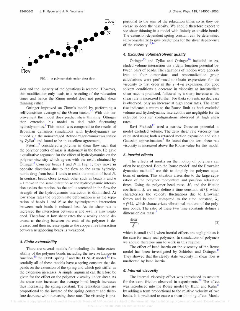
Peterlin9 considered a polymer in shear flow such thatthe polymer center of mass is stationary in the flow. He gavea qualitative argument for the effect of hydrodynamics on thepolymer viscosity which agrees with the result obtained byÖttinger.5 Consider beads 1 and N in Fig. 1; they move inopposite directions due to the flow so the extra hydrody-namic drag from bead 1 tends to resist the motion of bead N.In contrast beads close to each other such as beads n and n+1 move in the same direction so the hydrodynamic interac-tion assists the motion. As the coil is stretched in the flow thestrength of the hydrodynamic interaction is diminished. Atlow shear rates the predominate deformation is in the sepa-ration of beads 1 and N so the hydrodynamic interactionbetween such beads is reduced first. As the shear rate isincreased the interaction between n and n+1 is also weak-ened. Therefore at low shear rates the viscosity should de-crease as the drag between the ends of the polymer is de-creased and then increase again as the cooperative interactionbetween neighboring beads is weakened.

3. Finite extensibility

There are several models for including the finite exten-sibility of the polymer bonds including the inverse Langevinfunction,10 the FENE spring,11 and the FENE-P model.12 Es-sentially all of these models have a spring constant that de-pends on the extension of the spring and which gets stiffer asthe extension increases. A simple argument can therefore begiven for the effect on the polymer viscosity under shear. Asthe shear rate increases the average bond length increasesthus increasing the spring constant. The relaxation times areproportional to the inverse of the spring constant and there-fore decrease with increasing shear rate. The viscosity is pro-

portional to the sum of the relaxation times so as they de-crease so does the viscosity. We should therefore expect tosee shear thinning in a model with finitely extensible bonds.The extension-dependent spring constant can be determinedself-consistently to give predictions for the shear dependenceof the viscosity.13,14

4. Excluded volume/solvent quality

Öttinger15 and Zylka and Öttinger16 included an ex-cluded volume interaction via a delta function potential be-tween pairs of beads. The equations of motion were general-ized to four dimensions and renormalization groupcalculations were performed to obtain expressions for theviscosity to first order in the �=4−d expansion. For goodsolvent conditions a decrease in viscosity at intermediateshear rates is predicted, followed by a sharp increase as theshear rate is increased further. For theta solvents no decreaseis observed, only an increase at high shear rates. The sharprise indicates a return to the Rouse limit as both excludedvolume and hydrodynamic interactions are negligible for theextended polymer configurations observed at high shearrates.

Ravi Prakash17 used a narrow Gaussian potential tomodel excluded volume. The zero shear rate viscosity wascalculated using both a retarded motion expansion and via aGaussian approximation.7 He found that the zero shear rateviscosity is increased above the Rouse value for this model.

5. Inertial effects

The effects of inertia on the motion of polymers canoften be neglected. Both the Rouse model2 and the Browniandynamics method18 use this to simplify the polymer equa-tions of motion. This situation arises due to the large sepa-ration of the polymer momentum and position relaxationtimes. Using the polymer bead mass, M, and the frictioncoefficient, �, we may define a time constant, M /�, whichcharacterizes the velocity fluctuations due to Brownianforces and is small compared to the time constant, �H

=� /4k, which characterizes vibrational motions of the poly-mer bonds. The ratio of these two time constants defines adimensionless mass19

4kM

�2 , �3�

which is small ��1� when inertial effects are negligible as isthe case for many real polymers. In simulations of polymerswe should therefore aim to work in this regime.

The effect of bead inertia on the viscosity of the Rousemodel has been investigated by Schieber and Öttinger.19

They showed that the steady state viscosity in shear flow isunaffected by bead inertia.

6. Internal viscosity

The internal viscosity effect was introduced to accountfor the extra friction observed in experiments.20 The effectwas introduced into the Rouse model by Kuhn and Kuhn21

by adding a term proportional to the relative velocity of twobeads. It is predicted to cause a shear thinning effect. Manke

FIG. 1. A polymer chain under shear flow.

194906-2 J. F. Ryder and J. M. Yeomans J. Chem. Phys. 125, 194906 �2006�

This article is copyrighted as indicated in the article. Reuse of AIP content is subject to the terms at: http://scitation.aip.org/termsconditions. Downloaded to IP:

155.97.178.73 On: Mon, 06 Oct 2014 06:57:42

and Williams22 showed that shear thinning was delayed tohigher shear rates as the solvent viscosity is increased whilethe solvent quality is held fixed at the theta point. They con-cluded that this delay was due to the internal viscosity effect.

B. Experimental findings

Only recently has it been possible to view single poly-mers in flow. Smith et al.23 and LeDuc et al.24 used videofluorescence microscopy to study single DNA molecules inshear flow. They observed the DNA molecules tumbling inthe shear flow, extending and contracting, and formingdumbbell and hook shapes. They explained this behavior bydecomposing the shear flow into an elongational and a rota-tional flow of equal magnitude. In the elongational flow thepolymer would be extended along the elongational axis,whereas in the rotational flow it would form a coil andtumble in the flow. In shear flow these two states competegiving the random tumbling and coiling motions.

The experimental study of the non-Newtonian viscosityof polymer solutions began over 50 years ago �see, for ex-ample, Ref. 25�. The majority of polymer solutions and meltsare observed to shear thin, the viscosity decreases with in-creasing shear rate, but some show the opposite effect ofshear thickening. Obviously it is very difficult experimen-tally to isolate and identify the different factors causing thisbehavior.

Making use of the recent progress in imaging singleDNA molecules23,24 it is now possible to measure the viscos-ity of single molecules. Teixeira et al.26 measured elementsof the radius of gyration tensor in the flow-gradient planeand using the Giesekus expression for the stress tensor27 re-lated these to the viscosity. They observed a shear thinningeffect with a power law dependence on the shear rate���̇−0.52.

C. Numerical work

Various simulation methods have been used to studypolymers under shear flow. The most common is the Brown-ian dynamics method28 but some authors have used nonequi-librium molecular dynamics29 and most recently dissipativeparticle dynamics.30

Aust et al.29 used nonequilibrium molecular dynamicssimulations to study polymers under shear. This simulationmethod includes a full description of the solvent, so it is verydemanding on computational resources. Therefore no viscos-ity calculations were performed because it is difficult to runsimulations over the necessary time period to obtain suchmeasurements. Instead the authors study the rotation and de-formation of the polymer in the flow and observe the variousmotions observed in experiments by Smith et al.23 andLeDuc et al.24

Comparisons have been made between the results ofSmith et al.23 for polymer expansion and motion in shearflow and Brownian dynamics simulations by Hur andShaqfeh31 and Jendrejack et al.32 There is a good agreementbetween experiment and simulation. Other authors havecompared the expansion of chains calculated via Browniandynamics to light scattering results on polystyrene in dioctyl

phthalate �DOP�.33 They found that both simulation andtheory overestimated the expansion observed in the experi-ments.

Knudsen et al.34 calculated the radius of gyration ofGaussian chains with hydrodynamics included via the Rotne-Prager-Yamakawa tensor both with and without excludedvolume. In the absence of the excluded volume interactionfor low shear rates Rg matched the equilibrium value pre-dicted by the Rouse model. As the shear rate was increasedRg decreased before returning to the Rouse value. If the ex-cluded volume interaction was included, as would be ex-pected, at low shear rates Rg was greater than the Rousevalue. It then decreased as the shear rate was increased tobelow the Rouse value before eventually returning to theRouse value for the largest shears.

Brownian dynamics simulations have also been used tostudy polymer viscosity. The effect of the finite extensibilityof polymer chains has been investigated by a number of au-thors using a FENE potential.32,35–37 All conclude that itcauses shear thinning. The effect of excluded volume haslikewise received much attention via either a Gaussianpotential,37,38 a 1 /r12 potential,39 or an exponentialpotential.34 Again the agreement is that the excluded volumeinteraction causes shear thinning at low shear rates but, asthe polymer becomes more extended and the effect becomesnegligible, the viscosity reaches a plateau at the Rouse value.The hydrodynamic interaction is included in such simula-tions via either the Oseen tensor or the Rotne-Prager-Yamakawa tensor. It is observed to cause a shear thickeningeffect until, as with the excluded volume interaction, the vis-cosity returns to the Rouse value at high shear.34,36

Schroeder et al.40 used the Brownian dynamics methodwith hydrodynamics included using the Rotne-Prager-Yamakawa tensor to model an excluded volume wormlikechain. The simulation results are compared to the experimen-tal results obtained in Ref. 26. With a suitable choice ofsimulation parameters they found an excellent agreement.

Pan and Manke30 used the dissipative particle dynamicsmodel41 to study short polymer chains �N=10� with a FENEpotential.11 Dissipative particle dynamics models the solventby explicit particles so it includes hydrodynamic effects. Theeffects of solvent quality can be taken into account by choos-ing the interaction parameters of the conservative force ap-propriately. They obtained the polymer viscosity for a rangeof shear rates for good, theta, and bad solvents. The polymeris observed to shear thin for all three solvent conditions, thethinning being most pronounced in a good solvent.

II. THE MODEL

A. Solvent model

The solvent is modeled using the multiparticle collisiondynamics algorithm introduced in Ref. 42. This is a particlebased method for solving the equations of fluctuating hydro-dynamics. The system consists of N particles of mass m withposition ri and velocity vi. The particles are distributed ran-domly within a simple cubic lattice of size LxLyLz, with anumber density �=N /LxLyLz, which is divided into cubic

194906-3 Shear thinning in polymer solutions J. Chem. Phys. 125, 194906 �2006�

This article is copyrighted as indicated in the article. Reuse of AIP content is subject to the terms at: http://scitation.aip.org/termsconditions. Downloaded to IP:

155.97.178.73 On: Mon, 06 Oct 2014 06:57:42

cells of side a. The evolution of the system occurs in discretetime steps of duration �t. Each time step consists of a freestreaming step and a collision step.

The positions of the particles are first updated in thestreaming step according to

ri�t + �t� = ri�t� + vi�t��t . �4�

The particle velocities are then updated within the collisionstep. First, the particles are grouped according to the cubiccell they are occupying. The velocity of the center of massVc.m. of the cell is then calculated and the velocities of theparticles in that cell are transformed according to

vi�t + �t� = Vc.m. + ��vi�t� − Vc.m.� , �5�

where � is a rotation matrix randomly selected from a set ofmatrices that perform a rotation of angle about a randomlychosen axis.

Performing the velocity transformation in the framemoving with the center of mass ensures that a system de-scribed by Eqs. �4� and �5� locally conserves both momen-tum and energy. The equilibrium velocity distribution of theparticles is given by the microcanonical ensemble and an Htheorem exists for the relaxation to equilibrium.42 The sim-plicity of the algorithm has allowed the transport coefficientsto be calculated analytically.43–46

In Ref. 47 it was shown that multiparticle collision dy-namics is not Galilean invariant at low temperatures. It wasargued that this was due to a breakdown of molecular chaos,the assumption that collisions are uncorrelated in space andtime. At low temperature the average particle velocity��kBT� is small and hence the mean free path is short��a�. As a result particles may remain in the same cell fromone time step to the next and therefore collide with the sameparticles repeatedly thus introducing unphysical memory ef-fects. This problem is improved by a modification of thealgorithm in which the grid of cells is shifted by a randomvector with components in the range �−a /2 ,a /2� at eachcollision. The procedure is most easily implemented by shift-ing the position of each particle by the same random vectorin this range before the collision step and then returning it toits original position after the collision.

Multiparticle collision dynamics has been used to studya number of different complex systems. For example, Pad-ding and Louis48 used the model to investigate the interplaybetween Brownian and hydrodynamic fluctuations in sedi-menting colloids, while Noguchi and Gompper49,50 studiedthe dynamics of fluid vesicles in shear flow. Most recentlyRipoll et al.51 have studied the behavior of star polymersunder shear flow.

B. Lees-Edwards boundary conditions

In order to introduce shear into the multiparticle colli-sion dynamics model we apply Lees-Edwards boundaryconditions.43,52 These boundary conditions produce a steadyshear flow while mimicking an infinite system. To produce aflow in the x direction with a gradient in y we must applyperiodic boundary conditions in x and z and a special bound-ary condition in y. Any particle that crosses the boundary y

=0 at r= �x ,y=0,z� is replaced by a particle at the boundaryy=Ly with position r= �x= �x+ut�mod Lx ,y=Ly ,z� and ve-locity v= �vx=vx+u ,vy ,vz� where mod denotes the use ofmodular arithmetic. Similarly if a particle leaves the upperboundary at r= �x ,y=Ly ,z�, it is replaced by a particle at thelower boundary with position r= �x= �x−ut�mod Lx ,y=0,z�and velocity v= �vx=vx−u ,vy ,vz�. This procedure produces asteady shear flow with a shear rate �̇=u /Ly. In shearing thesystem we are continually pumping energy into it. To main-tain a fixed temperature this energy must be removed by athermostatting process. In this work this is done by rescalingthe peculiar velocities, vpec=vi−vflow, of the particles. First,the temperature of the fluid is calculated using 3kT /m=m�vpec

2 � /2 and from this a scale factor is calculated, T /T0

where T0 is the desired temperature. This factor is then usedto rescale the peculiar velocities before adding back the bulkflow.

C. Polymer model

In order to investigate the various contributions to thebehavior of polymers under shear we consider several differ-ent bead-spring models for the polymer. The polymer equa-tions of motion are integrated using a standard moleculardynamics approach, the velocity Verlet algorithm, with timestep t.

1. Gaussian chain

The simplest model is a Gaussian chain. This model con-sists of beads of mass M connected via Gaussian springswith

VGauss�r� =k

2r2, �6�

where r is the distance between two adjacent beads and k isrelated to the equilibrium bond length. In all simulations thatfollow we will take k=10. When backflow �hydrodynamicinteractions between monomers� is absent this is simply theRouse model, with backflow it is approximated by the Öt-tinger model.

2. FENE chain

The Gaussian model is an unrealistic model of a polymerin that the bonds forming the polymer backbone can be ex-tended indefinitely. One way of modeling the finite extensi-bility of the polymer backbone is to replace the Gaussiansprings by FENE springs11 with

VFENE�r� = −k

2R0

2 ln1 − � r

R0�2 , r � R0, �7�

where R0 denotes the maximum extension of the spring. Asthe spring extension approaches R0 the attractive force be-tween the beads diverges. In the present work we take R0

=1.5� where � is the Lennard-Jones length parameter andwill be introduced in the next section.

194906-4 J. F. Ryder and J. M. Yeomans J. Chem. Phys. 125, 194906 �2006�

This article is copyrighted as indicated in the article. Reuse of AIP content is subject to the terms at: http://scitation.aip.org/termsconditions. Downloaded to IP:

155.97.178.73 On: Mon, 06 Oct 2014 06:57:42

3. Excluded volume chain

A Lennard-Jones potential is used to model the effects ofexcluded volume and solvent quality

VLJ�r� = � 4���

r�12

− ��

r�6 + � , r 21/6� ,

��4���

r�12

− ��

r�6 + �� , r � 21/6� .�

�8�

� is a measure of the solvent quality. In this work we willtake �=1 and �=1. When considering polymers in solutionthe solvent is described as either good, theta, or poor. For agood solvent the excluded volume interaction dominates andat equilibrium the polymer is in an extended state. In a poorsolvent interbead attraction dominates and the polymer isfound to be in a collapsed globular state. When the two in-teractions exactly balance we have a theta solvent. To modelthese effects we control the value of � in Eq. �8�. If �=0 theLennard-Jones interaction is purely repulsive. The polymer istherefore in an extended state and we are modeling a goodsolvent. For ��0 the Lennard-Jones potential has an attrac-tive tail for large r. As � is increased the strength of theattractive force increases until it dominates over the repulsivepart. The polymer at this stage is now in a collapsed state andwe are modeling a poor solvent. In the simulations that fol-low we take �=1.2 to mimic a bad solvent.

D. Polymer solvent coupling

The coupling of a polymer molecule to the multiparticlecollision dynamics solvent is straightforward.53 During thestreaming step of the solvent the molecular dynamics algo-rithm is run to update the position and velocity of the poly-mer. The polymer then takes part in the multiparticle colli-sion dynamics collision step. The center of mass velocity ofthe cell includes the contribution from any beads that may bein the cell,

Vc.m. =

�j

MjV j + �i

mivi

�j

Mj + �i

mi

, �9�

where j runs over all the polymer beads in the cell, i runsover all the solvent particles in the cell, and V j is the velocityof bead j. Both the polymer beads and the solvent particlesundergo the collision defined by Eq. �5� using the center ofmass velocity given in Eq. �9�. This allows the transfer ofmomentum and energy between the solvent and polymer.Through this exchange the polymer beads experience a dragforce which may be characterized by a friction coefficient, �,as calculated in Ref. 54.

The model includes the hydrodynamic interaction be-tween polymer beads. The strength of this interaction may becharacterized by the dimensionless number55

h* =�

�s� k

36�3kBT�2

, �10�

where �s is the solvent viscosity. When modeling polymersone would normally use 0�h*�0.3. In the present simula-tions of the Guassian chain h*=0.14 within the normalbounds. This value depends on the parameters used for thesolvent model through its dependence on � and �s.

E. Removal of the backflow effect

Backflow is the hydrodynamic interaction between poly-mer beads. In multiparticle collision dynamics there is a rela-tively straightforward procedure for removing this interac-tion facilitating a direct study of its effects. In order toremove the momentum correlations from the model we ran-domly interchange the solvent particle velocities after eachcollision step. In this way there is still global conservation ofmomentum but momentum conservation is destroyed locally.The solvent can no longer propagate hydrodynamic modesand therefore models a Brownian solvent. If there is shearflow then this procedure must be carried out on the peculiarvelocities.

F. Polymer viscosity

There are three contributions to the stress tensor neededto calculate the viscosity of the polymer molecule: a kineticcontribution from the motion of polymer beads, a collisionalcontribution due to the multiparticle collision step, and acontribution from the forces acting between polymer beads.

The kinetic contribution to the stress tensor for a poly-mer with N beads is given by

�xy,kin = −1

V�i=0

N

MiViy�Vix − vx�Ri�� , �11�

where V=LxLyLz is the volume of the simulation and vx�Ri�is the solvent velocity at the position of bead i.

The contribution due to the forces between the beads isgiven by1

�xy,force = −1

V�i=0

N

RixFiy , �12�

where Fiy is the y component of the force acting on bead idue to all the other beads and Rix is the x position of bead i.

Calculating the collisional contribution due to the poly-mer presents a problem because it cannot be separated fromthat due to the solvent. This can be seen as follows. Considera cell with only one polymer bead and n solvent particles. Aplane of constant y cuts the cell into two with the polymerbead being in the lower part. During the collision step mo-mentum is transferred between all particles in the cell, bothsolvent and polymer, and we wish to calculate how muchcrosses the plane. This can be done in two ways. We maycalculate the total momentum of those particles below theplane before and after the collision. The difference is then theamount which has crossed the plane. As the bead is belowthe plane we may find that its momentum has changed dur-ing the collision and hence we have a polymer contribution

194906-5 Shear thinning in polymer solutions J. Chem. Phys. 125, 194906 �2006�

This article is copyrighted as indicated in the article. Reuse of AIP content is subject to the terms at: http://scitation.aip.org/termsconditions. Downloaded to IP:

155.97.178.73 On: Mon, 06 Oct 2014 06:57:42

to �xy,col. On the other hand, we could have considered thechange in total momentum of those particles above the plane.In this case we would not get any polymer contribution to�xy,col. So all we can actually calculate is a combination ofthe polymer and solvent contributions. However, the colli-sional contribution to the viscosity with and without thepolymer was indistinguishable so in the results that follow itwill not be included.

III. FLEXIBLE POLYMERS UNDER SHEAR

We consider flexible chains and present results for theconfiguration and viscosity of linear polymers in shear flow.Following Pan and Manke30 we study a chain of length N=10 in a system of size 20�10�10 a3. The short chainlength allows for a realistic simulation time. The polymerwas allowed to reach equilibrium in the solvent for 10 000time steps, �t, before the shear boundary conditions wereapplied. The system was then allowed a further 10 000 timesteps to reach the steady state. At this stage the solvent ve-locity, density, and temperature profiles were checked to en-sure that the steady state had been reached. Measurementswere then taken over 100 000 time steps. All results are pre-sented in simulation units.

The solvent parameters were a=1, m=4, �t=1, �=10,kBT=1, and =3� /4. The polymer beads had mass M =16and the molecular dynamics time step was taken as 0.02�t.Parameters pertaining to specific polymer models were givenin Sec. II C.

Results for the polymer viscosity will be plotted againsta dimensionless quantity, the Weissenberg number. This issimply the product of the longest relaxation time of the poly-mer �1 and the applied shear rate

Wi = �1�̇ . �13�

The relaxation time of the polymer must be calculated nu-merically. One of the simplest ways of doing this is by look-ing at the decay of the correlations of the polymer radius ofgyration. The longest relaxation time is much larger than theothers ��p=�1 / p2 in the Rouse model where �p is the relax-ation time of the pth mode� and hence gives the dominantcontribution to the decay. A single exponential fit to the de-cay provides the estimates we require. The relaxation timesfor the different polymer models are listed in Table I.

A. Flexible polymer configuration in shear flow

First, we will consider the configuration and motion ofthe polymer in a shear flow. In equilibrium, in the absence offlow, the monomer distribution is spherical. If Wi�1 the

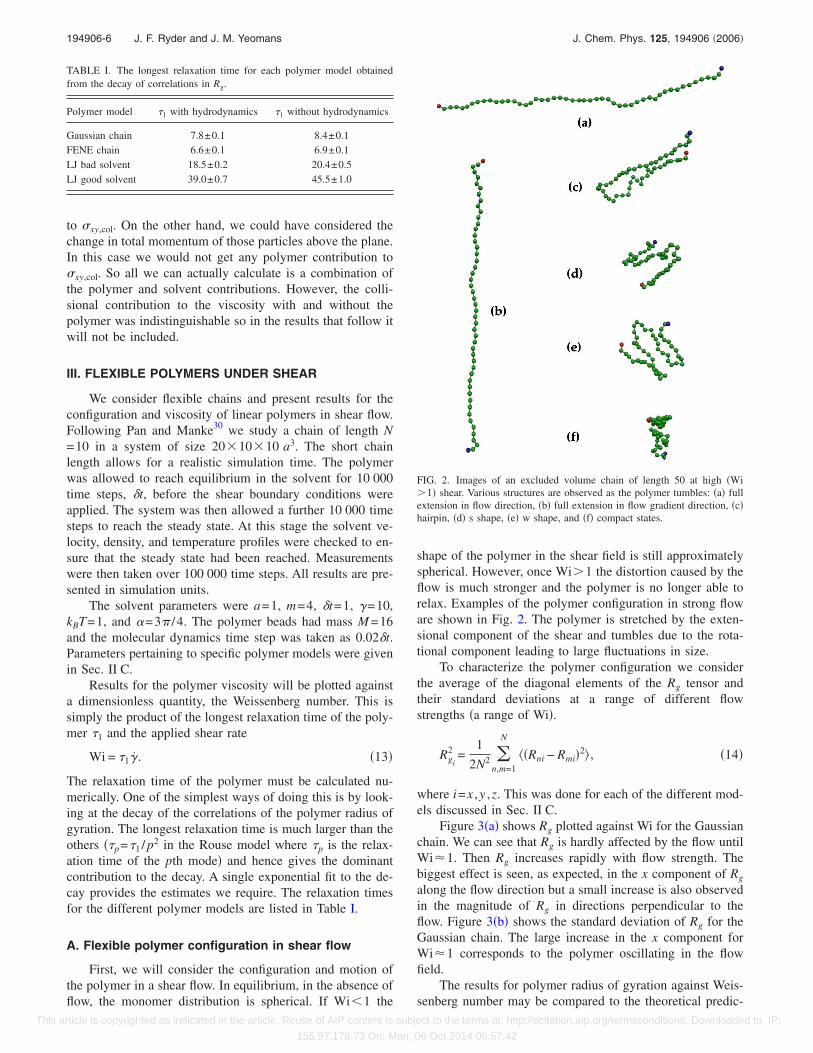
shape of the polymer in the shear field is still approximatelyspherical. However, once Wi�1 the distortion caused by theflow is much stronger and the polymer is no longer able torelax. Examples of the polymer configuration in strong floware shown in Fig. 2. The polymer is stretched by the exten-sional component of the shear and tumbles due to the rota-tional component leading to large fluctuations in size.

To characterize the polymer configuration we considerthe average of the diagonal elements of the Rg tensor andtheir standard deviations at a range of different flowstrengths �a range of Wi�.

Rgi

2 =1

2N2 �n,m=1

N

��Rni − Rmi�2� , �14�

where i=x ,y ,z. This was done for each of the different mod-els discussed in Sec. II C.

Figure 3�a� shows Rg plotted against Wi for the Gaussianchain. We can see that Rg is hardly affected by the flow untilWi�1. Then Rg increases rapidly with flow strength. Thebiggest effect is seen, as expected, in the x component of Rg

along the flow direction but a small increase is also observedin the magnitude of Rg in directions perpendicular to theflow. Figure 3�b� shows the standard deviation of Rg for theGaussian chain. The large increase in the x component forWi�1 corresponds to the polymer oscillating in the flowfield.

The results for polymer radius of gyration against Weis-senberg number may be compared to the theoretical predic-

TABLE I. The longest relaxation time for each polymer model obtainedfrom the decay of correlations in Rg.

Polymer model �1 with hydrodynamics �1 without hydrodynamics

Gaussian chain 7.8±0.1 8.4±0.1FENE chain 6.6±0.1 6.9±0.1LJ bad solvent 18.5±0.2 20.4±0.5LJ good solvent 39.0±0.7 45.5±1.0

FIG. 2. Images of an excluded volume chain of length 50 at high �Wi�1� shear. Various structures are observed as the polymer tumbles: �a� fullextension in flow direction, �b� full extension in flow gradient direction, �c�hairpin, �d� s shape, �e� w shape, and �f� compact states.

194906-6 J. F. Ryder and J. M. Yeomans J. Chem. Phys. 125, 194906 �2006�

This article is copyrighted as indicated in the article. Reuse of AIP content is subject to the terms at: http://scitation.aip.org/termsconditions. Downloaded to IP:

155.97.178.73 On: Mon, 06 Oct 2014 06:57:42

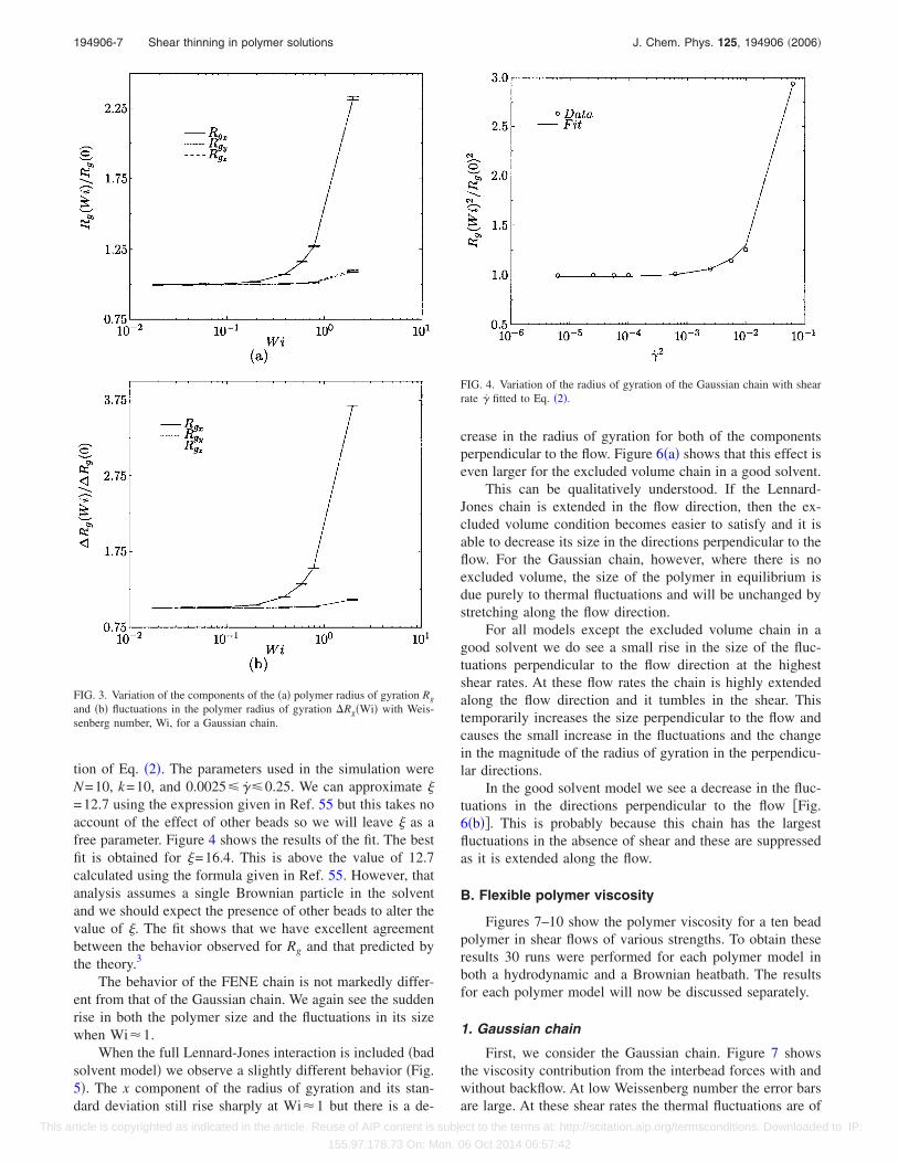
tion of Eq. �2�. The parameters used in the simulation wereN=10, k=10, and 0.0025 �̇ 0.25. We can approximate �=12.7 using the expression given in Ref. 55 but this takes noaccount of the effect of other beads so we will leave � as afree parameter. Figure 4 shows the results of the fit. The bestfit is obtained for �=16.4. This is above the value of 12.7calculated using the formula given in Ref. 55. However, thatanalysis assumes a single Brownian particle in the solventand we should expect the presence of other beads to alter thevalue of �. The fit shows that we have excellent agreementbetween the behavior observed for Rg and that predicted bythe theory.3

The behavior of the FENE chain is not markedly differ-ent from that of the Gaussian chain. We again see the suddenrise in both the polymer size and the fluctuations in its sizewhen Wi�1.

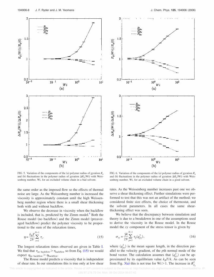
When the full Lennard-Jones interaction is included �badsolvent model� we observe a slightly different behavior �Fig.5�. The x component of the radius of gyration and its stan-dard deviation still rise sharply at Wi�1 but there is a de-

crease in the radius of gyration for both of the componentsperpendicular to the flow. Figure 6�a� shows that this effect iseven larger for the excluded volume chain in a good solvent.

This can be qualitatively understood. If the Lennard-Jones chain is extended in the flow direction, then the ex-cluded volume condition becomes easier to satisfy and it isable to decrease its size in the directions perpendicular to theflow. For the Gaussian chain, however, where there is noexcluded volume, the size of the polymer in equilibrium isdue purely to thermal fluctuations and will be unchanged bystretching along the flow direction.

For all models except the excluded volume chain in agood solvent we do see a small rise in the size of the fluc-tuations perpendicular to the flow direction at the highestshear rates. At these flow rates the chain is highly extendedalong the flow direction and it tumbles in the shear. Thistemporarily increases the size perpendicular to the flow andcauses the small increase in the fluctuations and the changein the magnitude of the radius of gyration in the perpendicu-lar directions.

In the good solvent model we see a decrease in the fluc-tuations in the directions perpendicular to the flow �Fig.6�b��. This is probably because this chain has the largestfluctuations in the absence of shear and these are suppressedas it is extended along the flow.

B. Flexible polymer viscosity

Figures 7–10 show the polymer viscosity for a ten beadpolymer in shear flows of various strengths. To obtain theseresults 30 runs were performed for each polymer model inboth a hydrodynamic and a Brownian heatbath. The resultsfor each polymer model will now be discussed separately.

1. Gaussian chain

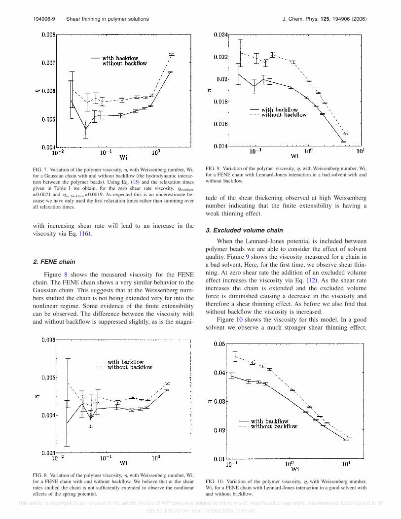
First, we consider the Gaussian chain. Figure 7 showsthe viscosity contribution from the interbead forces with andwithout backflow. At low Weissenberg number the error barsare large. At these shear rates the thermal fluctuations are of

FIG. 3. Variation of the components of the �a� polymer radius of gyration Rg

and �b� fluctuations in the polymer radius of gyration Rg�Wi� with Weis-senberg number, Wi, for a Gaussian chain.

FIG. 4. Variation of the radius of gyration of the Gaussian chain with shearrate �̇ fitted to Eq. �2�.

194906-7 Shear thinning in polymer solutions J. Chem. Phys. 125, 194906 �2006�

This article is copyrighted as indicated in the article. Reuse of AIP content is subject to the terms at: http://scitation.aip.org/termsconditions. Downloaded to IP:

155.97.178.73 On: Mon, 06 Oct 2014 06:57:42

the same order as the imposed flow so the effects of thermalnoise are large. As the Weissenberg number is increased theviscosity is approximately constant until the high Weissen-berg number region where there is a small shear thickeningboth with and without backflow.

We observe the decrease in viscosity when the backflowis included, that is, predicted by the Zimm model.4 Both theRouse model �no backflow� and the Zimm model �preaver-aged backflow� predict the polymer viscosity to be propor-tional to the sum of the relaxation times,

� =kBT

2V�s=1

N−1

�s. �15�

The longest relaxation times observed are given in Table I.We find that �no backflow��backflow so from Eq. �15� we wouldexpect �no backflow��backflow.

The Rouse model predicts a viscosity that is independentof shear rate. In our simulations this is true only at low shear

rates. As the Weissenberg number increases past one we ob-serve a shear thickening effect. Further simulations were per-formed to test that this was not an artifact of the method; weconsidered finite size effects, the choice of thermostat, andthe solvent parameters. In all cases the same shear-thickening effect was seen.

We believe that the discrepancy between simulation andtheory is due to a breakdown in one of the assumptions usedto derive the viscosity in the Rouse model. In the Rousemodel the xy component of the stress tensor is given by

�xy =�̇k

2V�p=1

N−1

�p�qpy2 � , �16�

where �qpy2 � is the mean square length, in the direction par-

allel to the velocity gradient, of the pth normal mode of thebond vector. The calculation assumes that �qpy

2 � can be ap-proximated by its equilibrium value kBT /k. As can be seenfrom Fig. 3�a� this is not true for Wi�1. The increase in Rgy

2

FIG. 5. Variation of the components of the �a� polymer radius of gyration Rg

and �b� fluctuations in the polymer radius of gyration Rg�Wi� with Weis-senberg number, Wi, for an excluded volume chain in a bad solvent.

FIG. 6. Variation of the components of the �a� polymer radius of gyration Rg

and �b� fluctuations in the polymer radius of gyration Rg�Wi� with Weis-senberg number, Wi, for an excluded volume chain in a good solvent.

194906-8 J. F. Ryder and J. M. Yeomans J. Chem. Phys. 125, 194906 �2006�

This article is copyrighted as indicated in the article. Reuse of AIP content is subject to the terms at: http://scitation.aip.org/termsconditions. Downloaded to IP:

155.97.178.73 On: Mon, 06 Oct 2014 06:57:42

with increasing shear rate will lead to an increase in theviscosity via Eq. �16�.

2. FENE chain

Figure 8 shows the measured viscosity for the FENEchain. The FENE chain shows a very similar behavior to theGaussian chain. This suggests that at the Weissenberg num-bers studied the chain is not being extended very far into thenonlinear regime. Some evidence of the finite extensibilitycan be observed. The difference between the viscosity withand without backflow is suppressed slightly, as is the magni-

tude of the shear thickening observed at high Weissenbergnumber indicating that the finite extensibility is having aweak thinning effect.

3. Excluded volume chain

When the Lennard-Jones potential is included betweenpolymer beads we are able to consider the effect of solventquality. Figure 9 shows the viscosity measured for a chain ina bad solvent. Here, for the first time, we observe shear thin-ning. At zero shear rate the addition of an excluded volumeeffect increases the viscosity via Eq. �12�. As the shear rateincreases the chain is extended and the excluded volumeforce is diminished causing a decrease in the viscosity andtherefore a shear thinning effect. As before we also find thatwithout backflow the viscosity is increased.

Figure 10 shows the viscosity for this model. In a goodsolvent we observe a much stronger shear thinning effect.

FIG. 7. Variation of the polymer viscosity, �, with Weissenberg number, Wi,for a Gaussian chain with and without backflow �the hydrodynamic interac-tion between the polymer beads�. Using Eq. �15� and the relaxation timesgiven in Table I we obtain, for the zero shear rate viscosity, �backflow

=0.0021 and �no backflow=0.0019. As expected this is an underestimate be-cause we have only used the first relaxation times rather than summing overall relaxation times.

FIG. 8. Variation of the polymer viscosity, �, with Weissenberg number, Wi,for a FENE chain with and without backflow. We believe that at the shearrates studied the chain is not sufficiently extended to observe the nonlineareffects of the spring potential.

FIG. 9. Variation of the polymer viscosity, �, with Weissenberg number, Wi,for a FENE chain with Lennard-Jones interaction in a bad solvent with andwithout backflow.

FIG. 10. Variation of the polymer viscosity, �, with Weissenberg number,Wi, for a FENE chain with Lennard-Jones interaction in a good solvent withand without backflow.

194906-9 Shear thinning in polymer solutions J. Chem. Phys. 125, 194906 �2006�

This article is copyrighted as indicated in the article. Reuse of AIP content is subject to the terms at: http://scitation.aip.org/termsconditions. Downloaded to IP:

155.97.178.73 On: Mon, 06 Oct 2014 06:57:42

This result agrees with that obtained by Pan and Manke30

using the dissipative particle dynamics method. It is alsoclear in Figs. 9 and 10 that as the Weissenberg number isincreased the effect of backflow becomes negligible. At suchhigh shear rates the imposed flow dominates the backflowand hence diminishes its effect.

IV. SEMIFLEXIBLE POLYMERS UNDER SHEAR

We now move to consider a semiflexible polymer inshear flow. Following Nogochi and Yoshikawa56 we model asemiflexible chain using a harmonic spring potential with anequilibrium length �,

Vbond =bkBT

2�2 ��Ri+1 − Ri� − ��2, �17�

and a three body bending potential

Vbend =skBT

2�1 +

�Ri−1 − Ri��Ri+1 − Ri��2 �2

. �18�

The parameter s controls the persistence length of the poly-mer. If s=0 and b is large the model approximates to aKramers bead-rod chain.1 In the case that both s and b arelarge the the model approximates to a multibead rod.1

Simulations were performed for a range of values of theparameter s corresponding to chains with different degrees offlexibility. First, we studied the model with s=0. This is aflexible chain similar to the Gaussian chain but the bondsnow have a finite equilibrium length �=1. The bending po-tential was then added with s= 5, 20, 40, 60, 120, and 400.The longest relaxation time for each model was calculated asdescribed in Sec. III and is given in Table II.

A. Semiflexible polymer configuration in shear flow

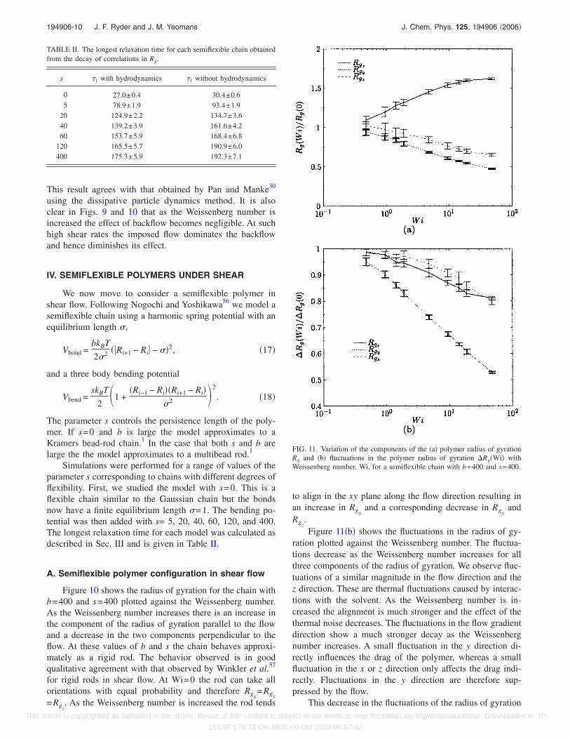
Figure 10 shows the radius of gyration for the chain withb=400 and s=400 plotted against the Weissenberg number.As the Weissenberg number increases there is an increase inthe component of the radius of gyration parallel to the flowand a decrease in the two components perpendicular to theflow. At these values of b and s the chain behaves approxi-mately as a rigid rod. The behavior observed is in goodqualitative agreement with that observed by Winkler et al.57

for rigid rods in shear flow. At Wi=0 the rod can take allorientations with equal probability and therefore Rgx

=Rgy=Rgz

. As the Weissenberg number is increased the rod tends

to align in the xy plane along the flow direction resulting inan increase in Rgx

and a corresponding decrease in Rgyand

Rgz.Figure 11�b� shows the fluctuations in the radius of gy-

ration plotted against the Weissenberg number. The fluctua-tions decrease as the Weissenberg number increases for allthree components of the radius of gyration. We observe fluc-tuations of a similar magnitude in the flow direction and thez direction. These are thermal fluctuations caused by interac-tions with the solvent. As the Weissenberg number is in-creased the alignment is much stronger and the effect of thethermal noise decreases. The fluctuations in the flow gradientdirection show a much stronger decay as the Weissenbergnumber increases. A small fluctuation in the y direction di-rectly influences the drag of the polymer, whereas a smallfluctuation in the x or z direction only affects the drag indi-rectly. Fluctuations in the y direction are therefore sup-pressed by the flow.

This decrease in the fluctuations of the radius of gyration

TABLE II. The longest relaxation time for each semiflexible chain obtainedfrom the decay of correlations in Rg.

s �1 with hydrodynamics �1 without hydrodynamics

0 27.0±0.4 30.4±0.65 78.9±1.9 93.4±1.9

20 124.9±2.2 134.7±3.640 139.2±3.9 161.6±4.260 153.7±5.9 168.4±6.8

120 165.5±5.7 190.9±6.0400 175.3±5.9 192.3±7.1

FIG. 11. Variation of the components of the �a� polymer radius of gyrationRg and �b� fluctuations in the polymer radius of gyration Rg�Wi� withWeissenberg number, Wi, for a semiflexible chain with b=400 and s=400.

194906-10 J. F. Ryder and J. M. Yeomans J. Chem. Phys. 125, 194906 �2006�

This article is copyrighted as indicated in the article. Reuse of AIP content is subject to the terms at: http://scitation.aip.org/termsconditions. Downloaded to IP:

155.97.178.73 On: Mon, 06 Oct 2014 06:57:42

for semiflexible chains is in contrast to the increase observedin the flexible chain. For a flexible chain we observed largefluctuations as the chain tumbled and expanded and con-tracted in the flow. In the case of a semiflexible chain thesemotions are suppressed by the bending potential.

B. Semiflexible polymer viscosity

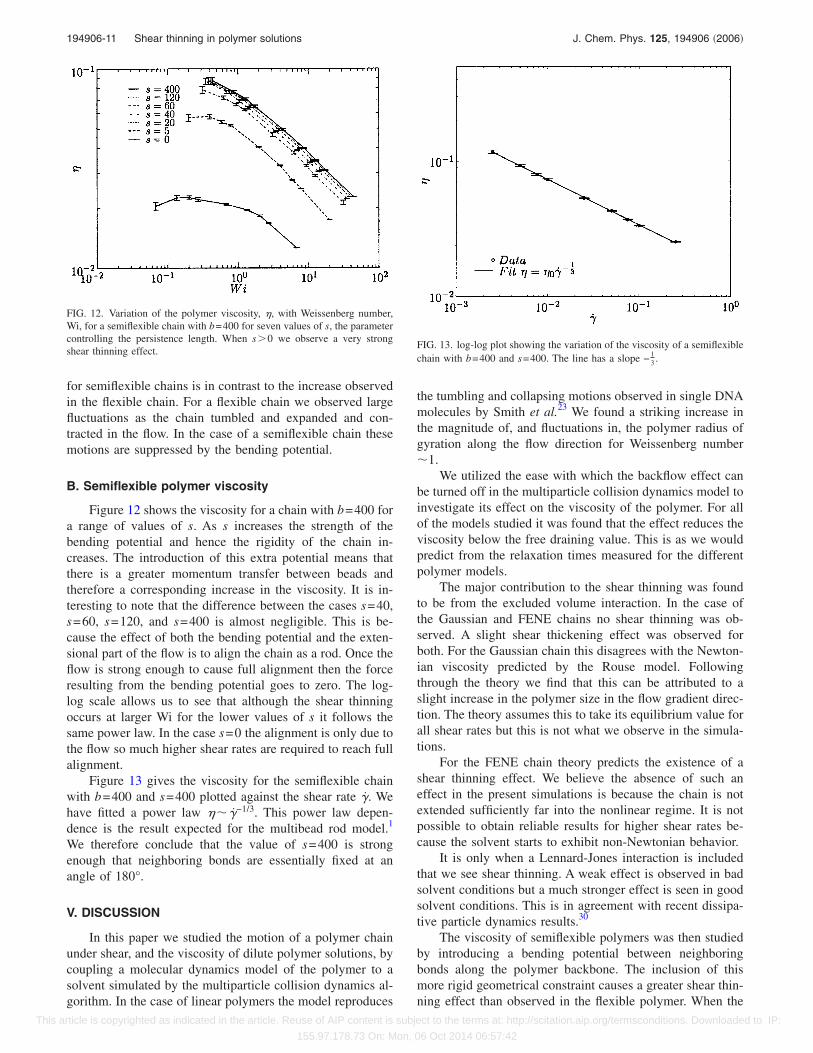
Figure 12 shows the viscosity for a chain with b=400 fora range of values of s. As s increases the strength of thebending potential and hence the rigidity of the chain in-creases. The introduction of this extra potential means thatthere is a greater momentum transfer between beads andtherefore a corresponding increase in the viscosity. It is in-teresting to note that the difference between the cases s=40,s=60, s=120, and s=400 is almost negligible. This is be-cause the effect of both the bending potential and the exten-sional part of the flow is to align the chain as a rod. Once theflow is strong enough to cause full alignment then the forceresulting from the bending potential goes to zero. The log-log scale allows us to see that although the shear thinningoccurs at larger Wi for the lower values of s it follows thesame power law. In the case s=0 the alignment is only due tothe flow so much higher shear rates are required to reach fullalignment.

Figure 13 gives the viscosity for the semiflexible chainwith b=400 and s=400 plotted against the shear rate �̇. Wehave fitted a power law �� �̇−1/3. This power law depen-dence is the result expected for the multibead rod model.1

We therefore conclude that the value of s=400 is strongenough that neighboring bonds are essentially fixed at anangle of 180°.

V. DISCUSSION

In this paper we studied the motion of a polymer chainunder shear, and the viscosity of dilute polymer solutions, bycoupling a molecular dynamics model of the polymer to asolvent simulated by the multiparticle collision dynamics al-gorithm. In the case of linear polymers the model reproduces

the tumbling and collapsing motions observed in single DNAmolecules by Smith et al.23 We found a striking increase inthe magnitude of, and fluctuations in, the polymer radius ofgyration along the flow direction for Weissenberg number�1.

We utilized the ease with which the backflow effect canbe turned off in the multiparticle collision dynamics model toinvestigate its effect on the viscosity of the polymer. For allof the models studied it was found that the effect reduces theviscosity below the free draining value. This is as we wouldpredict from the relaxation times measured for the differentpolymer models.

The major contribution to the shear thinning was foundto be from the excluded volume interaction. In the case ofthe Gaussian and FENE chains no shear thinning was ob-served. A slight shear thickening effect was observed forboth. For the Gaussian chain this disagrees with the Newton-ian viscosity predicted by the Rouse model. Followingthrough the theory we find that this can be attributed to aslight increase in the polymer size in the flow gradient direc-tion. The theory assumes this to take its equilibrium value forall shear rates but this is not what we observe in the simula-tions.

For the FENE chain theory predicts the existence of ashear thinning effect. We believe the absence of such aneffect in the present simulations is because the chain is notextended sufficiently far into the nonlinear regime. It is notpossible to obtain reliable results for higher shear rates be-cause the solvent starts to exhibit non-Newtonian behavior.

It is only when a Lennard-Jones interaction is includedthat we see shear thinning. A weak effect is observed in badsolvent conditions but a much stronger effect is seen in goodsolvent conditions. This is in agreement with recent dissipa-tive particle dynamics results.30

The viscosity of semiflexible polymers was then studiedby introducing a bending potential between neighboringbonds along the polymer backbone. The inclusion of thismore rigid geometrical constraint causes a greater shear thin-ning effect than observed in the flexible polymer. When the

FIG. 12. Variation of the polymer viscosity, �, with Weissenberg number,Wi, for a semiflexible chain with b=400 for seven values of s, the parametercontrolling the persistence length. When s�0 we observe a very strongshear thinning effect.

FIG. 13. log-log plot showing the variation of the viscosity of a semiflexiblechain with b=400 and s=400. The line has a slope − 1

3 .

194906-11 Shear thinning in polymer solutions J. Chem. Phys. 125, 194906 �2006�

This article is copyrighted as indicated in the article. Reuse of AIP content is subject to the terms at: http://scitation.aip.org/termsconditions. Downloaded to IP:

155.97.178.73 On: Mon, 06 Oct 2014 06:57:42

strength of the bending potential is large enough we find thatthe viscosity fits the prediction for a multibead rod. The fluc-tuations of the polymer Rg observed for the flexible chainsare suppressed for the rigid chain. The fluctuations resultedfrom thermal noise inducing a transition of the chain be-tween two unstable steady states. The effect of this noise iscounteracted by the bending potential for the semiflexiblechains and the transitions therefore do not occur.

As discussed in Sec. I C similar simulations are possibleusing the Brownian dynamics method.32–37 This method doesnot explicitly model the solvent; instead solvent effects areincluded by adding a drag term and a random term to theforces acting on the polymer beads. It is therefore a veryquick method to simulate polymer dynamics in the absenceof hydrodynamics. To include hydrodynamic effects theOseen tensor is used which depends on the relative positionsof all the beads in the system. As the chain size increases thecomputational cost of calculating the 3N2 elements of theOseen tensor58 increases rapidly. Given that the majority ofcomputing time is devoted to the solvent the time taken formultiparticle collision dynamics scales as the box size whichscales as Rg

3�N3� therefore one expects a crossover betweenthe time taken for the different simulation approaches as Nincreases. A comparison study of the two methods would bevery interesting but is beyond the scope of the present work.

1 R. B. Bird, R. C. Armstrong, and O. Hassager, Dynamics of PolymericLiquids �Wiley, New York, 1976�.

2 P. E. Rouse, J. Chem. Phys. 21, 1272 �1953�.3 H. L. Frisch, N. Pistoor, A. Sariban, K. Binder, and S. Fesjian, J. Chem.Phys. 89, 5194 �1988�.

4 B. H. Zimm, J. Chem. Phys. 24, 269 �1956�.5 H. C. Öttinger, J. Chem. Phys. 83, 6535 �1985�.6 H. C. Öttinger, J. Chem. Phys. 84, 4068 �1985�.7 H. C. Öttinger, J. Chem. Phys. 90, 463 �1988�.8 W. Zylka, J. Chem. Phys. 94, 4628 �1990�.9 A. Peterlin, J. Chem. Phys. 33, 1799 �1960�.

10 L. R. G. Treloar, The Physics of Rubber Elasticity �Clarendon, Oxford,1975�.

11 H. R. Warner, Ind. Eng. Chem. Fundam. 11, 125 �1972�.12 J. M. Weist and R. I. Tanner, J. Rheol. 33, 281 �1989�.13 F. Ganazzoli and A. Tacconelli, Macromol. Theory Simul. 7, 79 �1998�.14 F. Ganazzoli and A. Tacconelli, Macromol. Theory Simul. 8, 234 �1999�.15 H. C. Öttinger, Phys. Rev. A 40, 2664 �1989�.16 W. Zylka and H. C. Öttinger, Macromolecules 24, 484 �1991�.17 J. Ravi Prakash, Macromolecules 34, 3396 �2001�.18 D. L. Ermak and J. A. McCammon, J. Chem. Phys. 69, 1352 �1978�.19 J. D. Schieber and H. C. Ottinger, J. Chem. Phys. 89, 6972 �1988�.20 P.-G. de Gennes, Scaling Concepts in Polymer Physics �Cornell Univer-

sity Press, New York, 1979�.21 W. Kuhn and H. Kuhn, Helv. Chim. Acta 28, 1533 �1945�.22 C. W. Manke and M. C. Williams, Macromolecules 18, 2045 �1985�.23 D. E. Smith, H. P. Babcock, and S. Chu, Science 283, 1724 �1999�.24 P. LeDuc, C. Haber, G. Bao, and D. Wirtz, Nature �London� 399, 564

�1999�.25 T. Kotaka, H. Susuki, and H. Inagaki, J. Chem. Phys. 45, 2770 �1966�.26 R. E. Teixeira, H. P. Babcock, E. S. G. Shaqfeh, and S. Chu,

Macromolecules 38, 581 �2005�.27 Y.-H. Lin, Polymer Viscoelasticity �World Scientific, Singapore, 2003�.28 P. Dotson, J. Chem. Phys. 79, 5730 �1983�.29 C. Aust, S. Hess, and M. Kröger, Macromolecules 35, 8621 �2002�.30 G. Pan and C. W. Manke, J. Rheol. 46, 1221 �2002�.31 J. S. Hur and E. S. G. Shaqfeh, J. Rheol. 44, 713 �2000�.32 R. M. Jendrejack, J. J. de Pablo, and M. D. Graham, J. Chem. Phys. 116,

7752 �2002�.33 E. C. Lee and S. Muller, Polymer 40, 2501 �1999�.34 K. D. Knudsen, J. Garcia de la Torre, and A. Elgsaeter, Polymer 37, 1317

�1996�.35 J. J. López Cascales, F. G. Diaz, and J. Garcia de la Torre, Polymer 36,

345 �1995�.36 R. Pamies, M. C. Lopez Martinez, J. G. Hernandez Cifre, and J. Garcia

de la Torre, Macromolecules 38, 1371 �2005�.37 R. Prabhakar and J. Ravi Prakash, J. Non-Newtonian Fluid Mech. 116,

163 �2004�.38 K. Satheesh Kumar and J. Ravi Prakash, J. Chem. Phys. 121, 3886

�2004�.39 D. Petera and M. Muthukumar, J. Chem. Phys. 111, 7614 �1999�.40 C. M. Schroeder, R. E. Teixeira, E. S. G. Shaqfeh, and S. Chu,

Macromolecules 38, 1967 �2005�.41 P. J. Hoogerbrugge and J. M. V. A. Koelman, Europhys. Lett. 19, 155

�1992�.42 A. Malevanets and R. Kapral, J. Chem. Phys. 110, 8605 �1999�.43 N. Kikuchi, C. M. Pooley, J. F. Ryder, and J. M. Yeomans, J. Chem.

Phys. 119, 6388 �2003�.44 C. M. Pooley and J. M. Yeomans, J. Phys. Chem. B 109, 6505 �2005�.45 T. Ihle and D. M. Kroll, Phys. Rev. E 67, 066705 �2003�.46 T. Ihle and D. M. Kroll, Phys. Rev. E 67, 066706 �2003�.47 T. Ihle and D. M. Kroll, Phys. Rev. E 63, 020201�R� �2001�.48 J. T. Padding and A. A. Louis, Phys. Rev. Lett. 93, 220601 �2004�.49 H. Noguchi and G. Gompper, Phys. Rev. Lett. 93, 258102 �2004�.50 H. Noguchi and G. Gompper, Phys. Rev. E 72, 011901 �2005�.51 M. Ripoll, R. G. Winkler, and G. Gompper, Phys. Rev. Lett. 96, 188302

�2006�.52 A. W. Lees and S. F. Edwards, J. Phys. C 5, 1921 �1972�.53 A. Malevanets and J. M. Yeomans, Europhys. Lett. 52, 231 �2000�.54 N. Kikuchi, J. F. Ryder, C. Pooley, and J. M. Yeomans, Phys. Rev. E 71,

061804 �2005�.55 G. B. Thurston and A. Peterlin, J. Chem. Phys. 46, 4881 �1967�.56 H. Nogochi and K. Yoshikawa, J. Chem. Phys. 113, 854 �2000�.57 R. G. Winkler, K. Mussawisade, M. Ripoll, and G. Gompper, J. Phys.:

Condens. Matter 16, S3941 �2004�.58 M. Doi and S. F. Edwards, The Theory of Polymer Dynamics �Clarendon,

Oxford, 1986�.

194906-12 J. F. Ryder and J. M. Yeomans J. Chem. Phys. 125, 194906 �2006�

This article is copyrighted as indicated in the article. Reuse of AIP content is subject to the terms at: http://scitation.aip.org/termsconditions. Downloaded to IP:

155.97.178.73 On: Mon, 06 Oct 2014 06:57:42