Shear-Induced Aggregation- Fragmentation -

Shear-Induced Aggregation-Fragmentation: Mixing and Aggregate

Morphology Effects

A dissertation submitted to the

Division of Research and Advanced Studies of the University of Cincinnati

in partial fulfillment of the

requirements for the degree of

DOCTOR OF PHILOSOPHY

in the Department of Chemical Engineering of the College of Engineering

1997 by

Patrick Thomas Spicer

BChE, University of Delaware, 1992 MS, University of Cincinnati, 1995

Committee: Professor S. E. Pratsinis (Chair) Professor R. G. Jenkins Professor N. G. Pinto Dr. P. R. Mort

1

Table of Contents Chapter 1 - Literature Review .......................................................................................................4

Coagulation of Dilute Suspensions............................................................................................4 Laminar Shear – Rotational Flow.........................................................................................5 Turbulent Shear - Localized Flow .........................................................................................6

Collision Efficiency .....................................................................................................................9 Electrostatic Forces ................................................................................................................9 Structural Effects ...................................................................................................................9 Hydrodynamic Interactions .................................................................................................11 Simultaneous Orthokinetic and Perikinetic Coagulation..................................................14

Fragmentation in Dilute Suspensions.....................................................................................14 Fragmentation Rate .............................................................................................................14 Fragment Size Distribution.................................................................................................16

Simultaneous Aggregation-Fragmentation.............................................................................16 Aggregation-Fragmentation Steady State..........................................................................16 Shear-Induced Aggregate Restructuring ............................................................................16 Steady State Reversibility ...................................................................................................17

Sedimentation of Fractal Aggregates......................................................................................18 Concentrated Suspensions .......................................................................................................18

Concentrated Suspensions of Brownian Aggregates..........................................................18 Liquid-Liquid Dispersion: Coalescence- Breakage Systems..............................................19 Suspension Rheology............................................................................................................19 Shear-Induced Flocculation of Concentrated Suspensions................................................20 Characterization of Concentrated Suspensions .................................................................21

Conclusions ...............................................................................................................................24 Outline - Nonideal Effects ........................................................................................................25 Notation.....................................................................................................................................26

Greek Letters........................................................................................................................26 References .................................................................................................................................28

Chapter 2 - Time Lag for Steady State Attainment ...................................................................35 Introduction...............................................................................................................................36 Theory........................................................................................................................................37 Results and Discussion.............................................................................................................38

Development of the Steady State Floc Size Distribution...................................................38 Effect of Shear Rate on the Attainment of Steady State ...................................................39 Effect of Shear Rate Fluctuations on Steady State Attainment .......................................40

Conclusions ...............................................................................................................................42 Notation.....................................................................................................................................43


Chapter 3 - Effect of Impeller Type on Floc Size and Structure ................................................54 Introduction...............................................................................................................................55 Experimental.............................................................................................................................56

Apparatus and Procedure ....................................................................................................56 Stirred Tank Flow Field Characterization .........................................................................56 Floc Characterization by Image Analysis ...........................................................................57

Results and Discussion.............................................................................................................58 Impeller Flow Patterns and Circulation Time ...................................................................58 Effect of Impeller Type and Shear Rate on the Evolution of Floc Structure....................60

Conclusions ...............................................................................................................................60 Notation.....................................................................................................................................62


2

Chapter 4 - Effect of Shear Schedule on Particle Size and Structure .......................................77 Experimental.............................................................................................................................79 Results and Discussion.............................................................................................................81

Floc Size Distributions .........................................................................................................81 Floc Density and Structure..................................................................................................82 Practical Implications ..........................................................................................................83

Conclusions ...............................................................................................................................85 Acknowledgments .....................................................................................................................85 Notation.....................................................................................................................................86


Chapter 5 - Coagulation and Rotation of Aggregates in Shear Flow.......................................100 Introduction.............................................................................................................................101 Theory......................................................................................................................................102

Shear-Induced Particle Rotation and Collision ................................................................102 Simulated Fractal Aggregates...........................................................................................103

Experimental...........................................................................................................................104 Aggregate Rotation Experiments ......................................................................................104 Image Analysis ...................................................................................................................104

Results and Discussion...........................................................................................................104 Laminar Shear-Induced Aggregate Rotation ...................................................................104 Three-Dimensional Image Analysis Characterization of Polystyrene-Alum Aggregates105 Characterization of Simulated Fractal Aggregates .........................................................106 Coagulation Rate Expression Effects ................................................................................107

Conclusions .............................................................................................................................109 Acknowledgments ...................................................................................................................109 Notation...................................................................................................................................110

Greek Letters......................................................................................................................110 References ...............................................................................................................................111

Chapter 6 - Laminar and Turbulent Shear-Induced Flocculation of Fractal Aggregates......122 Introduction.............................................................................................................................123 Theory......................................................................................................................................123

Particle Size Distribution ..................................................................................................123 Aggregates ..........................................................................................................................124 Coagulation.........................................................................................................................124 Viscous Retardation of Collisions ......................................................................................125 Fragmentation ....................................................................................................................125

Experimental...........................................................................................................................126 Results and Discussion...........................................................................................................127

Effect of Aggregate Structure on Flocculation Kinetics...................................................127 Comparison with Experimental Data ...............................................................................128 Comparison with Literature Data.....................................................................................128

Conclusions .............................................................................................................................129 Acknowledgments ...................................................................................................................129 Notation...................................................................................................................................130

Greek Letters......................................................................................................................130 Chapter 7 - Concentrated Suspension Dynamics : Enhanced Backward Light Scattering ...139

Particle Characterization by Backward Light Scattering....................................................141 Experimental...........................................................................................................................141 Results and Discussion...........................................................................................................142 Conclusions .............................................................................................................................144 Acknowledgments ...................................................................................................................144 Notation...................................................................................................................................145

3


Chapter 8 - Modeling Shear-Induced Flocculation of Concentrated Suspensions..................153 Introduction.............................................................................................................................154 Theory......................................................................................................................................154

Population Balance Model .................................................................................................154 Results and Discussion...........................................................................................................155 Conclusions .............................................................................................................................157 Acknowledgments ...................................................................................................................157 Notation...................................................................................................................................158


Conclusions / Suggestions for Future Work ..............................................................................167 Appendices 1-9Appendix 1: Chapter 2 Computer Code............................................................168 Appendix 1: Chapter 2 Computer Code .....................................................................................169 Appendix 2: Chapter 5 Computer Code (Simulation) ...............................................................177 Appendix 3: Chapter 5 Computer Code (Analysis) ...................................................................187 Appendix 4: Chapter 6 Computer Code .....................................................................................193 Appendix 5: Chapter 8 Computer Code .....................................................................................212 Appendix 6 - Competition between Gas Phase and Surface Oxidation of TiCl4 during

Synthesis of TiO2 Particles .......................................................................................................220 Introduction.............................................................................................................................221 Theory......................................................................................................................................221 Results and Discussion...........................................................................................................223

Selection of Simulation Conditions ...................................................................................223 TiO2 Formation and Growth by Surface and Gas Phase Oxidation of TiCl4.................224 Effect of TiCl4 Mole Fraction, φ, and T on Titania Diameter..........................................225 Criteria for TiO2 Synthesis by Coagulation or Surface Growth .....................................226 Comparison with Experimental Results ...........................................................................227

Conclusions .............................................................................................................................227 Acknowledgments ...................................................................................................................228 References ...............................................................................................................................229

Appendix 7 – Appendix 6 Computer Code.................................................................................236 Appendix 8 – Gas Phase and Surface Oxidation of TiCl4 to form Polydisperse TiO2 .............243

Theory......................................................................................................................................245 Results and Discussion...........................................................................................................247

Model Validation and Selection of Simulation Conditions ..............................................247 Evolution of TiO2 Particle Size Distribution....................................................................248 Effect of Temperature on TiO2 Particle Diameter............................................................249 Comparison with Monodisperse Model Results ...............................................................250 Comparison with Alternative Models of Surface Oxidation ............................................250 Criteria for TiO2 Synthesis by Coagulation or Surface Growth ......................................250

Conclusions .............................................................................................................................251 Acknowledgments ...................................................................................................................251 References ...............................................................................................................................252

Appendix 9 – Appendix 8 Computer Code.................................................................................265

4

Chapter 1 - Literature Review

Coagulation of Dilute Suspensions Coagulation of particles can occur by Brownian motion (perikinetic coagulation), differential sedimentation, electric field interactions, and fluid shear (orthokinetic coagulation). Fluid shear-induced collisions are the most relevant mechanism of coagulation during most flocculation applications when particles are larger than 1 µm. Smoluchowski (1917) developed an expression for the collision rate of two particles i and j based on the velocity gradient, γ, experienced in laminar shear flow:

( )β γi j i ja a, = +43

3 (1-1)

where ai is the radius of particle i. Camp and Stein (1943) applied this work to turbulent flocculators using a “root mean square velocity gradient”, G, to characterize the distribution of shear rates in a stirred tank:

G =

ευ

1

2 (1-2)

by substituting G for γ in Equation (1-1):

( )βi j i jG a a, = +43

3 (1-3)

where ε is the turbulent energy dissipation rate and ν is the kinematic viscosity of the suspending fluid. Saffman and Turner (1956) derived the coagulation rate of neutrally buoyant particles smaller than the Kolmogorov microscale, η, in homogeneous, isotropic turbulence:

( )βi j i jG a a, .= +1293 (1-4)

It is interesting to note that the rigorous derivation of Saffman and Turner (1956) results in an expression that is nearly identical to the empirical work of Camp and Stein (1943). Equation (1-4) is the most widely used expression describing turbulent shear-induced coagulation and has been shown to be valid for a solids volume fraction, φ, up to 0.03-0.1 (Manley and Mason, 1955; Delichatsios and Probstein, 1975; Delichatsios, 1980; Brakalov, 1987). Expressions similar to Equation (1-4) have been derived using turbulent diffusivity arguments (Levich, 1962; Gruy and Saint-Raymond, 1997). From the above work, it appears that laminar and turbulent shear-induced coagulation are analogous. Recently, though, it has become evident that flocculation dynamics in the two flow regimes can differ significantly. Greene et al. (1994) compared the flocculation collision efficiency in different types of shear flow and concluded that the extrapolation of results for simple shear flow to describe more complex flows was not valid. Krutzer et al. (1995) compared experimental data for orthokinetic coagulation rates in simple shear flow, Taylor vortex flow, laminar pipe flow, and isotropic turbulent pipe flow with theoretical predictions. For all types of flow except Talyor vortex flow, experimental coagulation rates were smaller than theory predicted. They also concluded that particles coagulate most rapidly in isotropic turbulent flow at constant

5

energy dissipation rates because particles experience a lower shear rate, leading to less significant viscous retardation of collisions than for laminar flow (Krutzer et al., 1995).

Laminar Shear – Rotational Flow Laminar or simple shear provides a simple, idealized environment for the study of orthokinetic coagulation because particles suspended in laminar shear exhibit linear trajectories and their collision rate is well characterized by Equation (1-1) (Swift and Friedlander, 1964; Oles, 1992). Spherical particles in laminar shear flow are also known to exhibit rotational motion in the direction of travel with a constant angular velocity ω (Vand, 1948):

ωγ

=2

(1-5)

and a period of rotation T:

T =4πγ

(1-6)

Equations (1-5) and (1-6) assume spherical, suspended particles that follow the bulk fluid vorticity and were confirmed experimentally by Trevelyan and Mason (1951). Particle rotational motion is of interest in the study of suspension viscosity (as well as flocculation) because of its effect on particle collisions. Vand (1948) determined the fraction of time spent colliding for non-interacting spheres in simple shear that collide, rotate as a doublet, then separate:

t Na* = =163

43π φ (1-7)

Shear-induced particle rotation can induce lift in suspensions of neutrally buoyant particles, resulting in radial migration of particles in Couette flow, Poiseuille pipe flow, and in Couette flow at Reynolds numbers between Re = 4.6 x 104 and 9.2 x 104 (Ye and Roco, 1992). Suspensions under rotational flow can also exhibit enhanced thermal conductivity over the pure fluid. This results from enhanced convective heat transfer as the suspended particles rotate and continually transfer heat from the hot side to the cold side (Wang et al., 1989). Although the effect of particle rotation on spherical particles in simple shear is well understood, rotational motion by nonspherical particles becomes more complex and is only well understood for certain limiting cases. The rotation of asymmetric suspended particles is instrumental in determining preferred orientations and can affect suspension viscosity and thixotropy. Jeffery (1922) determined the rotation of rigid ellipsoids with major axis a and minor axis b in simple shear to have an angular velocity ω:

22

2222

basinbcosa

dtd

+θ+θ

γ=θ

=ω (1-8)

and a period of rotation T:

( )T

a bab

=+2 2 2πγ

(1-9)

Equations (1-8) and (1-9) reduce to Equations (1-5) and (1-6) for spheres (a = b). Trevelyan and Mason (1951) compared Equations (1-8) and (1-9) with observations of rotating cylindrical particles and found a smaller period of rotation for cylinders than predicted for ellipsoids, probably as a result of the differences in geometry.

The rotational characteristics of irregular, fractal flocs may not only affect the viscosity of a suspension but may also dictate the floc structures formed under shear. Torres et al. (1991) simulated the collisions of irregular aggregates linear and uniaxial extension

6

shear flow assuming aggregates followed the bulk fluid vorticity (Equation (1-5)) and concluded that aggregate rotation did not affect the structures formed. The assumption of bulk vorticity behavior may not convey the true character of anisotropic aggregate rotation. However, Torres et al. (1991) found statistically indistinguishable aggregate structures in simulated rotational and irrotational flow and concluded that aggregate structure is independent of flow features like rotation for non-interacting particles that form rigid bonds. Greene et al. (1994) showed that particle rotation created closed streamlines around particles, reducing particle collision rates for simple shear flow but had little effect for extensional flow. The assumption of spherical rotation rates for anisotropic aggregates is popular among simulations of bulk suspension properties as well, mainly because of a lack of quantitative data on anisotropic aggregate rotation (Brady and Bossis, 1985, 1988; Doi and Chen, 1989; Chen and Doi, 1989; Potanin, 1991).

Turbulent Shear - Localized Flow Turbulent shear, characterized by the presence of numerous fluid eddies, is frequently used to promote flocculation because of the resultant increases in momentum and mass transfer. By the classic Kolmogorov theory of turbulent flow, there is a cascade of energy from large eddies to the smallest eddies where kinetic energy is dissipated as heat by viscous forces (Batchelor, 1953). The characteristic length scale of these smallest eddies is given by the Kolmogorov microscale, η (Batchelor, 1953):

ηνε

=

31

4

(1-10)

The relative velocity of a particle with diameter d, ur, can be approximated by the root mean square (rms) relative velocity between two points a distance d apart in a fluid. The Kolmogorov theory of turbulence gives the magnitude of ur for particles larger and smaller than η:

u dr ∝

<εν

η

1

2 for (1-11)

( )u d dr ∝ >ε η1

3 for (1-12)

( )u L d Lr ∝ ≈ε1

3 for (1-13)

where L is the macroscale of the turbulent eddies (typically a characteristic length analogous to an impeller blade diameter). Typical values of η for practical G values used in flocculation (G = 30, 50, 100 s-1) are given by Equation (1-10) (η = 183, 141, 100 µm).

Equation (1-4) is frequently used to model coagulation of particles over a broad range of sizes and turbulent environments, though it is only accurate for particles smaller than η. For large particles experiencing vigorous turbulence, Abrahamson (1975) derived:

( )βi j i j i ja a v v, = + +52

2 2 (1-14)

where vi is the root mean square velocity of a floc of size i:

7

v vvi f

i

f

= +

−

1 15 2

1

2

.τ ε

(1-15)

and vf is the root mean square fluid velocity, a quantity that can be obtained from computational fluid dynamic simulations for a given application. Equation (1-14) assumes that the turbulence intensity is sufficiently large that the flow field in the stirred tank may be considered homogeneous (i.e. Re > 104). As a result, the suspended particles are flung randomly from eddy to eddy much as gas molecules move and collide. Equation (1-14) also requires that the flocs be in the macro subrange of turbulence (L/2 ≤ dp ∼ L). Equations (1-4) and (1-14) represent two extremes of particle behavior and are thus not universally applicable. Kruis and Kusters (1997), however, derived a universal expression for shear and acceleration-induced coagulation of particles in turbulent flow:

( )βπ

accel shear accel sheara a v v+ = + +83 1 2

2 2 2 (1-16)

where vaccel is the particle velocity relative to the fluid due to particle inertia (Saffman and Turner, 1956) and vshear the particle velocity relative to other particles due to fluid velocity gradients (Kruis and Kusters, 1997). At this level of detail in a turbulent stirred tank, fluid veloicites may be position-dependent and detailed information is required.

The flow field in a stirred tank is known to be homogeneous above an impeller Reynolds number, Rei:

ReiiND

=2

ν (1-17)

of 104, where Di is the impeller diameter. However, most practical flocculators are operated at Reynolds numbers well below 104 (Abrahamson, 1975). As a result, the turbulent flow field is heterogeneous and well characterized by a single G value only when particles are smaller than η (Cleasby, 1984). Cleasby (1984) suggested that the coagulation of particles larger than η correlated best with ε2/3 versus ε1/2 (i.e. Equation (1-4)) from calculations of the root mean square eddy velocity difference (Parker et al., 1972) and found good agreement with literature data. Clark (1985) criticized the approach by Camp and Stein (1943) of using a single G to characterize flocculation as the use of a single parameter to characterize a two-dimensional flow which in turn was used to approximate a three dimensional flow. He also suggested that while a mean velocity gradient that characterizes the average coagulation rate probably exists, the ability to calculate this quantity has not been demonstrated. Glasgow and Kim (1986) showed that the local turbulent energy dissipation rate can exceed the average value for a stirred tank by an order of magnitude depending on the impeller velocity. They emphasized that Equation (1-4) can underestimate the turbulence intensity in a stirred tank as a result of the large discrepancy between the region of the tank surrounding the impeller (impeller zone) and the rest of the tank (bulk zone). In light of the above findings, it will be necessary to characterize the heterogeneous flow in a stirred tank in order to accurately model flocculation. Shinnar (1961) suggested that based on the Kolmogorov theory of local isotropy, local turbulent energy dissipation rates are proportional to the average value, ε . Cutter (1966) observed two regions in a stirred tank, the bulk and the impeller zone. Tomi and Bagster (1978) estimated that the bulk zone comprises 90% of the stirred tank volume and that the turbulent energy dissipation rate in the bulk zone is 0.25 ε for a radial flow impeller. The turbulent energy dissipation rate in the impeller zone is largest at the tips of the impeller and can be about 50 ε , whereas the remainder of the impeller zone is characterized by 5.4 ε (Tomi and Bagster, 1978). Based on observations of this type, it is logical to assume that a

8

model describing separate regions of a stirred tank would be more accurate than one assuming complete homogeneity. ∅degaard (1979) modeled the continuous flocculation of phosphate for non-ideal flow conditions using a mass balance over the primary particles lost by coagulation and formed by erosion from the flocs. The mixed tanks in series description (Levenspiel, 1962) was used to describe the residence time distribution in the flocculator. The model was in good agreement with experimental data and although a systematic study was carried out, the breakage description was too simplified to be applicable to practical flocculators. Koh et al. (1984) developed a monodisperse two-compartment model for coagulation with no fragmentation in a stirred tank and compared its predictions with models describing up to thirty compartments. They concluded that because of the rapid circulation in a stirred tank, a single compartment model of flocculation was sufficient to describe flocculation provided a volume averaged shear rate was used instead of the rms shear rate of Equation (1-2).

Koh et al. (1987) used a population balance model of flocculation that assumed α = 0 for the formation of very large particles in place of a floc fragmentation model. Their calculated coagulation rates showed no difference between the predictions of one- and two-compartment models when scaled by the volume averaged shear rate. Smit et al. (1994) found a similar result analytically, noting no effect of the degree of mixedness on the extent of shear-induced aggregation in a continuous flow system. The lack of fragmentation in the above models limits their applicability to practical systems and will likely induce deviation from the observed independence of flow field. Kim and Glasgow (1987) modeled flocculation using a Monte Carlo model that assumed completely random coagulation and fragmentation of flocs in turbulent flow. The model was in good agreement with experimental data on the average floc size but limited comparisons were carried out. Casson and Lawler (1990) examined the effect of mixing conditions on flocculation using an oscillating-grid flocculator that produced turbulent eddies of a controlled size. Their results indicated that the most significant contribution to flocculation was by eddies of a size comparable to that of the flocculating particles and that larger eddies had little or no effect. Kusters (1991) developed a model of flocculation that incorporated several aspects of the heterogeneous stirred tank flow field. He determined, as a function of particle size, the fraction of time that particles spend in the impeller region being broken up based on numerical particle tracking calculations and theoretical descriptions of the fluid eddy frequency. This expression was used to describe particle breakage frequencies and to reduce the coagulation rate to account for the times when breakage occurred (Kusters, 1991).

Recently, Seckler et al. (1995) studied stirred tank hydrodynamics using computational fluid dynamic (CFD) models coupled with a moment model of the particle size distribution during precipitation. The model identified specific regions of particle formation in a precipitation reactor. This type of model would be equally valuable for the description of a flocculation process but no known work has coupled CFD with flocculation models.

Actual studies of aggregate structure formation have also been performed as a function of flow field. Torres et al. (1991) simulated aggregate formation in shear flow assuming spherical rotation characteristics and described hydrodynamic interactions using a model similar to that of Kusters et al. (1996). They found aggregates formed by CCA had a Df = 1.8, identical to that of aggregates formed by thermal motion. Apparently fluid particle interactions do not affect aggregate structure formation in simple shear flow. Muzzio and Ottino (1988) and Danielson et al. (1991) simulated aggregate formation in two-dimensional regular and chaotic flows. They found more compact structures were formed when heterogeneous systems had stagnant regions that allowed a transition from CCA to MCA mechanisms (Danielson et al., 1991). Hansen and Ottino (1996) modeled non-interacting fractal aggregate formation in two- and three-dimensional heterogeneous flows and observed enhanced collisions between aggregates versus spheres and aggregate structures that became more compact with increasing mixedness.

9

Collision Efficiency Equation (1-1) provides a baseline for the calculation of spherical particle collision frequencies that assumes a perfectly homogeneous flow field and no influence of electrostatic or viscous forces. Application of this coagulation model to a system violating any of these assumptions may cause a deviation from the predicted behavior and an inaccurate result. One efficient way to incorporate these nonidealities into a theoretical description of coagulation is to utilize a collision efficiency. This method describes the fraction of collisions that occur relative to those that would have occurred in an ideal system when Equation (1-1) was completely applicable. The relevant nonidealities and methods of accounting for them are reviewed below.

Electrostatic Forces The particles in most suspensions possess a net charge as a result of charged groups on their surface. The oppositely charged ions in the suspending fluid are attracted to these groups and form a layer around the surface of the particles. Charge conservation requires that the net charge on the particles be balanced by these ions because the suspension does not possess a net charge. Moving away from the surface of the particles, the concentration of the counterions sharply decreases and finally reaches a point where the solution is neutral. The charge on the particle creates a potential between the particle and the solution. The result is a repulsive force between the particles that prevents their mutual approach to distances close enough (5-10 nm) for the attractive van der Waals forces to bring the particles together irreversibly. Such a suspension is said to be electrostatically stable and will not coagulate without some additional step. The addition of a salt produces charged ions that reduce the effective distance of the electrostatic interactions. This is accomplished by increasing the solution ionic strength and suppressing the thickness of the layer of ions surrounding the particles. Around an ionic concentration of 0.1 M the thickness of the double layer is reduced to the extent that particles can approach close enough for the attractive van der Waals forces to dominate. At this point the suspension is destabilized and the particles will coagulate and form flocs if brought together by thermal motion or fluid shear. Particles can also be destabilized with charged polymers that adsorb to the particle surface and create a bridge between particles to form flocs. Similarly, the addition of Al2(SO4)3 16 H2O, or alum, causes Al(OH)3 to precipitate heterogeneously onto the particle surface and homogeneously in solution (Dentel and Gossett, 1987, 1988; Dentel, 1988, 1991). In either case the result is a decreased electrostatic repulsion between particles. The destabilizing agent (flocculant) allows the particles to come close enough together to adhere. Typical flocculants include alum and numerous polymers. In most practical cases, the reduction in collision efficiency resulting from electrostatic effects is negligible if sufficient flocculant has been added.

Structural Effects Flocs form irregular structures as a result of the random collisions of particles (Vold, 1963; Meakin, 1988; Amal et al., 1990 a,b, 1992; Torres, 1991a,b). Whereas coalescing droplets form perfect spheres upon collision, solid particles become increasingly porous as aggregates collide and water is incorporated into the structure of the aggregates (Tambo, 1991). Aggregate structure can be quantified using the concepts of fractal geometry (Mandelbrot, 1987). For a fractal-like aggregate comprised of i primary particles, its radius of gyration (average distance from the aggregate center of mass to each primary particle), Rg,

10

and the primary particle radius, a, are related by (Cohen and Wiesner 1990; Jiang and Logan, 1991):

i kR

ag

D f

=

0 (1-18)

where k0 is a proportionality constant or lacunarity, and Df is the mass fractal dimension of the floc. A Df = 3 indicates a spherical floc, a Df = 1 is characteristic of a linear chain of particles, and values between 1 and 3 are characteristic of irregular objects like aggregates, islands, and clouds (Mandelbrot, 1987). Based on Equation (1-18) and the definition of the characteristic length used by Saffman and Turner (1956) to derive Equation (1-4), the shear-induced collision frequency of flocs with a fractal structure is given by (Tambo and Watanabe, 1979; Jiang and Logan, 1991; Kusters, 1991; Wiesner, 1992):

β γi jD Dk a i jf f

, = +

43 0

3

1 1 3

(1-19)

where i is the number of primary particles comprising an aggregate of size i and a is the radius of a primary particle. The earliest attempt to incorporate aggregate structure into coagulation-fragmentation flocculation models was by Tambo and Watanabe (1979). Their approach was similar to modern fractal theories of aggregate structure but few calculations were performed with the model and no fundamental study was carried out. Developments in fractal geometry provided a means of quantifying the structure of irregular aggregates (Mandelbrot, 1987; Meakin, 1988). Kusters et al. (1991) showed theoretically that as flocs became less compact (decreasing fractal dimension) they coagulated more rapidly than volume equivalent spheres as a result of their increased collision profile. Torres et al. (1991a) modeled pure coagulation by theoretically monitoring the changes in the maximum (collision) radius and the hydrodynamic radius of the flocs versus the traditional monitoring of the (spherical) volume equivalent floc radius. They observed reasonable agreement of the model with experimental measurements of laminar shear-induced polystyrene flocculation with an electrolyte only after including a simplified form of breakage into their model.

Wiesner (1992) modeled the first few minutes of a flocculation process when breakage is minimal using a population balance model incorporating the structure of the flocs into the collision frequency expression. His model showed that more irregular flocs grew faster than their volume equivalent spherical counterparts (i.e. Equation (1-1) and was in good agreement with Kusters et al. (1991; 1996) but neither model accounted for floc breakage. The current level of modeling of fractal aggregate flocculation behavior is able to account for flocs with a constant fractal dimension that do not fragment. The bulk of practical systems, however, evolve with respect to size and structure and fragment frequently. Equation (1-18) is extremely dependent on the choice of k0, the lacunarity of the fractal aggregates under consideration. This parameter is not well defined and may not be well represented by ideal simulations of aggregate structure, at least for aerosol agglomerates that sinter (Neimark et al., 1996). Because experimental data typically exist for a single fractal dimension and no known simulations have been carried out over a broad range of aggregate structures, it is unclear how k0 relates to Df. This information, though, is required to accurately describe fractal aggregation kinetics and a characteristic aggregate length for use in Equation (1-1).

11

Hydrodynamic Interactions Most theoretical descriptions of flocculation utilize classical descriptions of the suspension that assume a homogeneous flow field, spherical coalescent particles, and no particle-particle interactions during particle collisions. As two particles approach one another to collide, there is a viscous resistance associated with the thinning of the liquid film between them. For orthokinetic and perikinetic coagulation, this resistance will prevent particle contact completely unless a rapidly increasing attractive force such as the van der Waals interaction brings the particles together (Spielman, 1978; Delichatsios, 1980). A significant number of fundamental studies have been carried out on the magnitude of viscous retardation of coagulation for simple particle systems. Spielman (1970) quantified the effect of viscous interactions on the Brownian coagulation of two spherical particles by recalculating the diffusivity of the particles incorporating the fluid forces exerted on each particle. For thin double layers, the viscous effects were found to retard coagulation rates by as much as a factor of ten but to be relatively insignificant when larger repulsive forces were in effect. When double layer repulsion may be ignored, as is the case when sufficient electrolyte is present, the viscous effects were canceled by the van der Waals forces. Curtis and Hocking (1970) experimentally measured the efficiency of collisions of particles in simple shear flow by comparison with a monodisperse model and observed decreasing collision efficiencies (55-32%) with increasing shear rates (0.6-112 s-1). Van de Ven and Mason (1977a) found theoretically that for negligible electrostatic repulsion, the rate of binary collisions was proportional to γ0.82 (as opposed to Equation (1-1)) and that collision efficiency decreased with increasing shear rates. Zeichner and Schowalter (1977) calculated a dependency of collision frequency on γ0.77 for simple shear flow and γ0.86 for uniaxial extensional flow for values of the dimensionless parameter NF:

Na

AF =6 3πµ γ

(1-20)

larger than 10, where A is the Hamaker constant. Equation (1-20) represents the ratio of the hydrodynamic and to the attractive van der Waals forces. While the above studies were concerned with collisions between particles of the same size (monodisperse), Adler (1981a) showed theoretically that this type of coagulation was favored over the coagulation of different sized particles (polydisperse) in shear flow. Higashitani (1982) followed Adler’s procedure to calculate particle collision efficiencies for polydisperse coagulation. He used these values in a population balance model and found that Equation (1-1) overpredicted the rate of coagulation compared with the predictions incorporating hydrodynamic effects. This theory was applied to turbulent coagulation by Higahsitani (1983) and compared with experimental data for coagulation in a stirred tank. Comparison of the data with the predictions of Equation (1-4) indicated that hydrodynamic interactions reduce the turbulent coagulation rate. De Boer et al. (1989a) observed decreasing collision efficiencies during turbulent shear-induced coagulation of polystyrene particles with NaCl and attributed it to hydrodynamic interactions. Casson and Lawler (1990) concluded there was no effect of larger particles on the growth of smaller particles during controlled turbulent coagulation experiments using different particle sizes. Han and Lawler (1992) extrapolated the collision efficiency calculations of Adler (1981a) and compared the relative significance of different modes of flocculation by assuming additivity of the fluid shear, Brownian motion, and differential settling mechanisms. Fluid shear was significant only when both particles were larger than 1 µm and whose sizes varied no more than an order of magnitude. These results were qualitatively confirmed by the experimental data of Lawler (1993), who found significantly reduced collisions between large and small particles. Adachi et al. (1994) inferred that hydrodynamic interactions reduced the dependency of turbulent collision rates

12

on the primary particle diameter to d02.46 from d03. Brunk et al. (1997) examined turbulent coagulation of particles smaller than η experiencing hydrodynamic and electrostatic interactions by direct numerical simulation and trajectory calculations. They observed up to a 50% decrease in collision rates relative to Equation (1-4) as a result of particle-particle and particle-fluid interactions at intermediate turbulent strain rates. All of the above studies were carried out assuming spherical, nonporous particles. The flocs produced in an industrial flocculator, however, can be highly porous and may deviate from such descriptions. Adachi (1995) suggested that structural effects may negate or largely reduce the hydrodynamic interactions between porous flocs relative to those experienced by impermeable spheres. Wolynes and McCammon (1977) concluded theoretically that the hydrodynamic interactions between coagulating porous spheres were much less significant than for rigid, solid spheres. Adler (1981b) modeled flow in and through porous spheres based on the Brinkman equation of motion and found increased collision efficiency (reduced hydrodynamic interactions) with porosity. Torres et al. (1991a) developed an expression for the collision efficiency of porous flocs by taking into account the reduction of hydrodynamic and attractive forces on porous relative to impermeable particles and concluded that assuming completely successful collisions (α = 1) produced little error. Chellam and Wiesner (1993) calculated flow through porous fractal aggregates and suggested that the approach detailed above for impermeable spheres was accurate for application to the collisions of flocs with fractal dimensions, Df, ≥ 2.3. Veerapaneni and Wiesner (1996) developed a form of the shear-induced collision frequency accounting for the effects of viscous retardation for fractal aggregates with radially varying permeability:

( )β ψ ψi j i i j jG d d, = +16

3

(1-21)

where ηi is the collision efficiency of a particle of size i. The parameter ψi is a function of the ratio of the force exerted by fluid on a permeable floc to that exerted on an impermeable floc, and is independent of Df (Veerapaneni and Wiesner, 1996). Clearly, the influence of hydrodynamic interactions is to retard the collision of particles and this effect itself may be retarded by flow through porous particles. Kusters et al. (1996) extended the model of Adler (1981a) by assuming that porous flocs comprised of spherical primary particles only experience the hydrodynamic interactions of the two primary particles in each floc closest to each other. In addition, reduction of viscous effects by flow through the flocs was determined by modeling the floc as comprised of a porous shell and an impermeable core. This model predicts a reduction in viscous effects with decreasing Df as a result of increased floc porosity and accurately predicts experimental floc size evolution when coupled with a description of fractal aggregate collisions for both laminar and turbulent flow (Kusters et al., 1996). The above models all rely on some form of porosity expression to model fluid-aggregate interactions under the assumption that some fluid will permeate an aggregate and influence its behavior. However, Potanin (1991) calculated an expression for aggregate collision efficiencies by assuming aggregates were impermeable to flow and was able to match experimental literature data well. This indicates the uncertainty of the exact coagulation phenomenon because of the difficulty in direct experimental investigations. In addition, the observation that aggregates rotate under shear flow may further complicate descriptions assuming idealized flow through porous aggregates and point to the need for more complex descriptions of aggregate hydrodynamic behavior. For example, if an aggregate rotates (versus remaining in a fixed orientation) as it moves through a shear field, then flow patterns through or around the aggregate will deviate significantly from those around a fixed object. In Stokes flow, the total drag force exerted on a sphere with radius a by the surrounding fluid is given by (Lamb, 1943):

13

F Ua= 6πµ (1-22)

where U and µ are the fluid velocity and viscosity, respectively. It is convenient to substitute the radius of a sphere experiencing the same drag as the aggregate, RH, for a in Equation (1-22) to define:

RF

UH =6πµ

(1-23)

Wiltzius (1987) evaluated colloidal silica by light scattering and determined the ratio of the aggregate hydrodynamic radius to its radius of gyration, RH/Rg = 0.72 for Df = 2.1 in agreement with linear polymer chains in solution (RH/Rg = 0.79) and simulation results (Chen et al., 1987) giving RH/Rg = 0.79 - 0.97. Pusey et al. (1987) corrected this finding slightly to RH/Rg = 0.82 - 1.08. Rogak and Flagan (1990) found that RH/Rg varied from 0.89 for Df = 1.8 to 1.0 for Df = 2.1 and was determined by the largest length scales of an aggregate. For example, a linear chain of aggregates with Df = 2.1 had an RH/Rg << 1 despite the compact individual aggregate structures.

The inclusion of aggregate porosity in the estimation of aggregate hydrodynamic radii was used by van Saarloos (1987) and Kusters et al. (1996) to analytically relate the outer or collision radius of an aggregate, Rc, to its radius of gyration, Rg, by:

RD

DRc

f

fg=

+ 2 2 (1-24)

and RH to Rc by (Kusters et al., 1996):

RR

H

c

=−

+ −

−

− −

1

132

32

1

2 3

ξ ξ

ξ ξ ξ

tanh( )

tanh( ) (1-25)

where:

ξκ

=Rc (1-26)

and κ is the aggregate permeability with dimensionless density ρ :

κρ ρ ρ

ρ ρ=

− + −

+

392

92

3

9 3 22

1

3

5

3 2

5

3

2

Ca

s

(1-27)

and Cs is a shielding coefficient equal to 0.5 for aggregates and 0.724 for doublets. Although existing work describes the effect of hydrodynamic interactions on aggregation kinetics, no known study has examined the effect of hydrodynamic interactions on the type of aggregate structures formed in shear flow. Johnson et al. (1996) determined values of RH/Rg = 0.5 – 0.05 for Df = 1.79 – 2.25 from aggregate settling measurements. This significant variation from the above simulation results indicates the inadequacy of existing aggregate porosity models at describing practical aggregate systems.

14

Simultaneous Orthokinetic and Perikinetic Coagulation Swift and Friedlander (1964) analyzed the kinetics of simultaneous orthokinetic and perikinetic coagulation by assuming the two mechanisms were additive. They found good agreement of a monodisperse model with experimental data for the coagulation of polystyrene particles. Van de Ven and Mason (1977b) solved the convective diffusion equation for particles around a reference particle for values of the Peclet number, Pe:

Pea G

kT=

3 3πµ (1-28)

less than 1, where µ is the fluid viscosity, k is Boltzmann’s constant and T is absolute temperature. They gave an expression for collision rate that predicted results smaller than by the additivity result, with the discrepancy increasing with particle size. Zeichner and Schowalter (1979) found that for a ratio of shear- to Brownian-induced collision frequencies < 5 and γ < 400 s-1, Brownian coagulation affected (enhanced) shear-induced coagulation. They did, however, note that shear controlled the coagulation rate for all shear rates (100-1800 s-1) and concluded that Brownian collisions were important only for particles brought close together by shearing. Feke and Schowalter (1983) considered shear-dominated coagulation when small amounts of Brownian coagulation are present and concluded that Equation (1-1) could under-predict the shear-induced coagulation rate for values of the Peclet number, Pe < 290 and over-predict it for Pe > 290.

Han and Lawler (1992) assumed additivity of different flocculation mechanisms and calculated that Brownian motion was relevant during flocculation only when at least one of the colliding particles is less than 1 µm in diameter. Adachi et al. (1994) studied the initial rates of turbulent coagulation of polystyrene particles using a standardized mixing procedure involving the pouring of a suspension from one vial to another. From comparisons with a monodisperse model, they concluded that Brownian and shear coagulation rates were additive. Kusters et al. (1996) found that polydisperse coagulation models assuming additivity most accurately matched experimental data for turbulent coagulation.

Fragmentation in Dilute Suspensions As flocs grow larger, they become increasingly porous as a result of the random mechanism of coagulation and the inclusion of water in the floc structure. As they continue to grow and approach the length scales of turbulent eddies, hydrodynamic stresses can act upon these more fragile flocs and fragment them. These stresses are manifested as two mechanisms of floc breakage: splitting and erosion. Instantaneous velocity differences across the body of the floc produce splitting: the production of several floc fragments of a size similar to the parent floc (Thomas, 1964; Kusters, 1991). In addition, fluid drag forces can strip primary particles or small clusters of them from the surface of the floc, called erosion (Parker et al., 1972). Erosion has been shown to disturb the asymptotic scaling behavior of particle size distributions (Hansen and Ottino, 1996). Turbulent velocity fluctuations in the viscous subrange (dp < η) result in shearing of the floc, while in the inertial and macro ranges of turbulence (L> dp > η and dp ≈ L) pressures normal to the surface of the floc can split it.

Fragmentation Rate Parker et al. (1972) suggested an expression for the maximum floc diameter, dmax, that can resist breakage in a shear field characterized by G:

15

dC

GCa

a

max = =

2

νε

(1-29)

where C and a are constants determined by the floc characteristics. Equation (1-29) is often used to correlate experimental data on the maximum floc size. Kusters (1991) theoretically compared the two mechanisms of floc breakage and determined that splitting was dominant, in agreement with experimental findings (Akers et al., 1987). In the viscous and inertial subrange, the rate of fragmentation by splitting of a particle of radius ai is given by (Delichatsios and Probstein, 1976; Kusters, 1991):

Su

au

uii

b=

−

21

2 2

2π∆ ∆

∆exp (1-30)

where ∆u is the rms velocity difference across the floc diameter and ∆ub is the critical velocity difference above which breakage of the floc occurs. Substituting into Equation (1-30) for ∆u and ∆ub gives the simplified form of the breakage rate (Kusters, 1991):

Sib=

−

415

12

12

πεν

εε

exp (1-31)

where εb is the critical turbulent energy dissipation rate above which flocs are fragmented. The εb decreases with increasing floc size as a result of increasing porosity (Tambo and Watanabe, 1979; Sonntag and Russell, 1987; Kusters, 1991) and may be obtained from experimental data by rearrangement of Equation (1-29):

εb i

ia

dA

d( ) = 1 (1-32)

where A is C1/aν. The structure of a floc determines its strength and thus the probability it will fragment during shearing. Sonntag and Russell (1986; 1987) showed that shear-induced flocculation produced flocs with a self-similar fractal structure and that the variation of the porosity radially within the floc could be described using fractal concepts. They theoretically developed a criterion for the critical energy dissipation rate based on the structure of the floc. This model was later derived in an analogous form by Kusters (1991) based on similar theory:

( )ε

ρµb

n Dkd f

=−2 3

(1-33)

where n is 2.5 based on rheological measurements (Sonntag and Russel, 1986) and k is a fitting parameter. Blunt (1989) showed that there is a broad distribution of hydrodynamic forces on the surface of a fractal aggregate in shear flow. He found that the largest forces are exerted at the extreme tips of the aggregate, while flow is stagnant in the internal regions between the protruding tips, indicating a high fragmentation probability at weak points based on the concentration of force at relatively few points.

Horwatt et al. (1992) simulated the simple shear flow breakage of model fractal agglomerates using Monte Carlo techniques. They found that a model incorporating the irregularity of the agglomerate structure decreased the predicted critical stress at which fragmentation occurred by an order of magnitude versus models based on fracture tests of powder compacts of the material. Williams et al. (1992) suggested that more compact floc

16

structures were more likely to suffer erosion whereas more open flocs would break by splitting. Potanin (1993) simulated the shear-induced fragmentation of fractal aggregates in shear flow using a Monte Carlo model and compared shear-induced fragmentation of “soft” aggregates with central interactions that do not resist small deformations and “rigid” aggregates that react elastically to shearing based on their internal structure. His results bracketed existing experimental work, indicating a combination of soft and rigid characteristics of actual aggregates.

Fragment Size Distribution The number of fragments produced when a floc fragments significantly affects the contribution of fragmentation to a flocculation process (Spicer and Pratsinis, 1996). Because flocculation is a coagulation-fragmentation process, the fragment size distribution will also largely determine the steady state floc size distribution that is attained. Binary breakage, the production of two fragments of equal size, is a popular modeling assumption (Fair and Gemmell, 1964; Grabenbauer and Glatz, 1981; Burban et al., 1989; Chen et al., 1990). Various standard fragment size distributions like the normal (Coulaloglou and Tavlarides, 1977; Alvarez et al., 1994) and the lognormal (Peng and Williams, 1994) have also been used during modeling of coagulation-fragmentation processes. Kusters (1991) modeled flocs fragmentation by assuming that two unequal fragments were produced. Monte Carlo simulations of aggregate fragmentation indicated the production of two or more fragments by shearing with the mean daughter aggregate size an inverse power function of shear rate (Potanin, 1992; 1993). These fragments were denser than the parent aggregate and no direct relationship was found between parent and daughter structure. Glasgow and Luecke (1980) reasoned that fragmentation could not produce a single fragment size since flocs formed by collision of primary particles with primary particles, primary particles with flocs, and flocs with flocs. They observed experimentally that splitting was the dominant form of fragmentation. Pandya and Spielman (1982) observed the production of 2-3 daughter fragments during floc fragmentation in uniaxial extensional flow. De Boer et al. (1989b) and Kusters (1991) observed the production of floc fragments one third and one fourth the size of the parent floc, respectively, during the stirred tank flocculation of polystyrene with NaCl.

Simultaneous Aggregation-Fragmentation

Aggregation-Fragmentation Steady State Blatz and Tobolsky (1945) developed one of the earliest models of aggregation-

fragmentation by assuming breakage at any of the links in a linear chain of particles was equally probable. Spicer and Pratsinis (1996) used a population balance model to show that broadening the fragment size distribution (from binary to ternary to normal) broadened the steady state aggregate size distribution but did not alter the self-preserving nature of that distribution.

Shear-Induced Aggregate Restructuring Any shearing of irregular flocs is likely to produce compaction as particle-particle

bonds shift to positions with higher coordination numbers. This can happen even when fragmentation does not occur, numerical simulations of this process produced a change in aggregate fractal dimension, Df , from 1.89 to 2.13 (Jullien and Meakin, 1989). Shear-

17

induced coagulation simulations excluding any restructuring produce fractal clusters with Df = 1.8 (Torres et al., 1991) while experimental shear-induced coagulation-fragmentation processes produce small aggregates with Df = 2.1 and large aggregates with Df = 2.5 (Oles, 1992; Kusters et al., 1996). The shift from Df = 1.8 to 2.1 probably results from shear-induced reorganization while the shift from Df = 2.1 to 2.5 is likely brought about by more intense restructuring during fragmentation-regrowth cycles that occur as the larger aggregates interact more with the small eddies. As aggregates pass through regions of high and low shear rates in a stirred tank, both reorganization and restructuring occur. Restructuring is likely the most prevalent compaction mechanism when a steady state is reached between coagulation and fragmentation during flocculation. The bulk of aggregate structural characterization has been performed on a mass basis by sedimentation and light scattering techniques. However, surface morphology will also affect particle interactions. Image analysis techniques allow aggregate boundary and thus surface characterization (Mandelbrot et al., 1984). Bower et al. (1997) fragmented lactose aggregates in laminar shear, decreasing the fragment boundary fractal dimension, Dbf, from 1.4 to 1.3. This indicates a decrease in the compactness of the aggregate boundary/surface with fragmentation, in agreement with observations of the perimeter based fractal dimension, Dpf, (Spicer et al., 1996) although aggregate fragments are known to be more dense than the parent structure on a mass basis (Akers, 1987; Oles, 1992). The effect of prolonged shear exposure is increased aggregate density and surface area.

Steady State Reversibility A change in the applied shear rate drives a suspension at steady state to a new

steady state. By lowering or raising the shear rate, larger or smaller flocs are formed, respectively. After the second steady state has been attained, if the original shear rate is then re-applied, two types of behavior have been observed experimentally: reversible and irreversible. For particle suspensions destabilized with an ionic salt (i.e. NaCl), when the original shear rate is re-applied, the steady state average floc size returns to its original steady state value. These suspensions exhibit reversible floc dynamics because floc fragmentation and regrowth does not affect the van der Waals binding forces between primary particles (Kusters, 1991). Current flocculation models agree with these data, indicating that the steady state floc size distribution (FSD) for reversible systems is independent of initial conditions (Chen et al., 1990).

When the flocculant is a precipitated solid (i.e. Al(OH)3) or polymer, the suspension exhibits irreversible floc dynamics. Francois (1987) studied kaolin-Al(OH)3 floc fragmentation and regrowth at various shear rates in stirred tanks. In all cases, flocs regrew but did not attain their previous steady state average size. He explained this as floc formation by a multi-level progression: primary particles combined to form dense microflocs, which in turn combined to form the next level and so on. Leu and Ghosh (1988) flocculated kaolin suspensions with a polyelectrolyte and observed a similar behavior: flocs were reformed after intense fragmentation but did not attain their original steady state average size. They attributed this to the detachment of polymer chains from kaolin particles, resulting in a reduced collision efficiency and, thus, smaller particles. Clark and Flora (1991) studied cycled-shear flocculation of polystyrene-Al(OH)3 flocs by analysis of floc microphotographs. The flocs, formed at Gf = 35 s-1, fragmented at Gb = 150-1800 s-1 and re-formed at Gr = 35 s-1, exhibited increasingly compact structures but no clear size variation trend was observed. Glasgow and Liu (1995) found that kaolin-polymer flocs were more dense following cycled-shear flocculation with cycled introduction of additional flocculant.

Cycled shear application can most easily be envisioned as a macroscopic application of the shear history of individual flocs in a stirred tank that pass through alternating low and high shear zones. As a result, this technique may provide information regarding

18

aggregate-shear interactions in turbulent flow fields that result from aggregate irreversibilities.

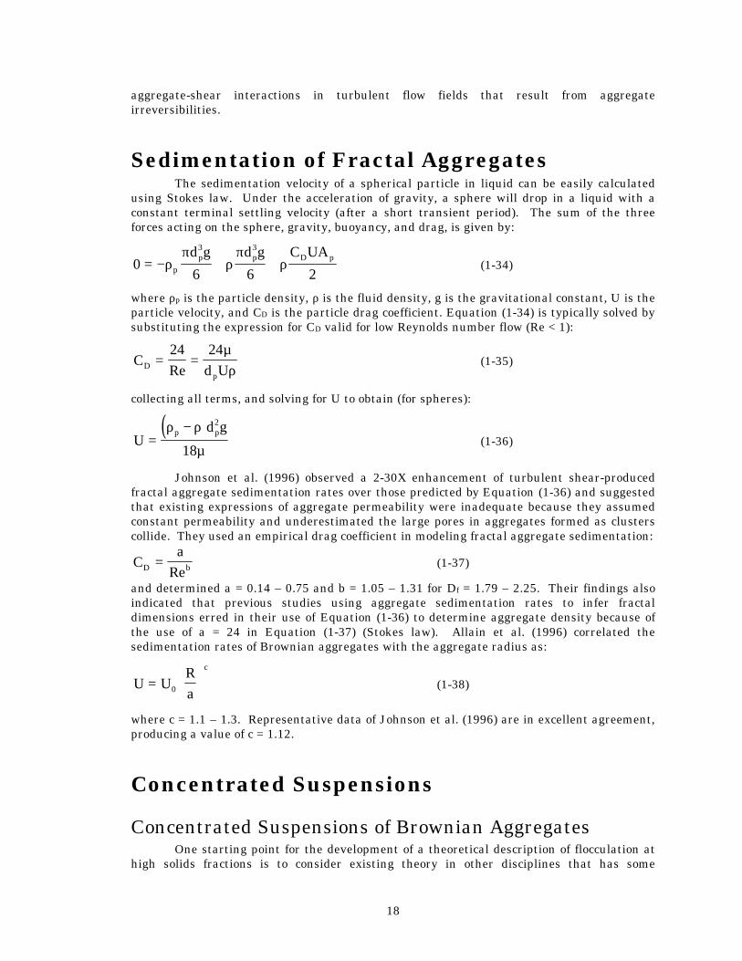
Sedimentation of Fractal Aggregates The sedimentation velocity of a spherical particle in liquid can be easily calculated using Stokes law. Under the acceleration of gravity, a sphere will drop in a liquid with a constant terminal settling velocity (after a short transient period). The sum of the three forces acting on the sphere, gravity, buoyancy, and drag, is given by:

06 6 2

3 3

= − + +ρπ

ρπ

ρpp p D pd g d g C UA

(1-34)

where ρp is the particle density, ρ is the fluid density, g is the gravitational constant, U is the particle velocity, and CD is the particle drag coefficient. Equation (1-34) is typically solved by substituting the expression for CD valid for low Reynolds number flow (Re < 1):

Cd UD

p

= =24 24Re

µρ

(1-35)

collecting all terms, and solving for U to obtain (for spheres):

( )U

d gp p=

−ρ ρ

µ

2

18 (1-36)

Johnson et al. (1996) observed a 2-30X enhancement of turbulent shear-produced fractal aggregate sedimentation rates over those predicted by Equation (1-36) and suggested that existing expressions of aggregate permeability were inadequate because they assumed constant permeability and underestimated the large pores in aggregates formed as clusters collide. They used an empirical drag coefficient in modeling fractal aggregate sedimentation:

Ca

D b=Re

(1-37)

and determined a = 0.14 – 0.75 and b = 1.05 – 1.31 for Df = 1.79 – 2.25. Their findings also indicated that previous studies using aggregate sedimentation rates to infer fractal dimensions erred in their use of Equation (1-36) to determine aggregate density because of the use of a = 24 in Equation (1-37) (Stokes law). Allain et al. (1996) correlated the sedimentation rates of Brownian aggregates with the aggregate radius as:

U URa

c

=

0 (1-38)

where c = 1.1 – 1.3. Representative data of Johnson et al. (1996) are in excellent agreement, producing a value of c = 1.12.

Concentrated Suspensions

Concentrated Suspensions of Brownian Aggregates One starting point for the development of a theoretical description of flocculation at high solids fractions is to consider existing theory in other disciplines that has some

19

relevance to the case under study. The number of existing investigations into the coagulation of concentrated suspensions is small because of the large computational demands and the sparse experimental data. A large body of existing work deals with perikinetic diffusion and coagulation and provides insight into the types of interparticle interactions experienced at high solids loadings (Bensley and Hunter, 1983; Dickinson, 1984; Eschenazi and Papadopoulos, 1995). The synergy of particle mean free path effects and aggregation kinetics may be revealed from studies of aggregate structure at high solids fractions. Adachi and Ooi (1990) studied Brownian aggregates of polystyrene particles and found Df increased from 2.0 to 2.2 as the initial solids volume fraction was increased from φ = 1.7 x 10-5 to 0.004. They attributed this shift to an increased packing density as a result of the decreased void spaces available, although caution must be used when interpreting fractal dimension data as a result of its inherent error of ± 0.1 (Kusters et al., 1996).

Liquid-Liquid Dispersion: Coalescence- Breakage Systems Research into dispersion behavior regularly investigates the shear-induced coalescence and breakage of suspended liquid droplets at volume fractions as high as φ = 0.5. As a result, one possible resource for the development of theoretical models of flocculation at high solids loadings is the dispersion literature. However, the turbulent energy required to maintain a two phase dispersion is significantly higher than that used during flocculation.

Suspension Rheology

Viscous Behavior of Suspensions The rheological behavior of a flocculated suspension will be a function of the floc size and structure distribution within the suspension. Creating a suspension by adding particles to a fluid can alter the magnitude of the viscosity but can also result in all known deviations from Newtonian flow. In a flocculated suspension, shear can alter the floc structures and produce a viscoelastic response as the elastic interaction forces between flocs oppose flow. These effects are most significant above a volume fraction of about φ = 0.01, when particles interactions increase, disturbing flow and increasing viscosity (Mewis and Macosko, 1994). Gillespie (1983) developed an empirical model to describe the effect of floc structure on suspension rheology but did little other than discuss means of obtaining the model parameters. Doi and Chen (1989) and Chen and Doi (1989) simulated the two- and three-dimensional aggregation-fragmentation of suspended spheres at high solids fractions (φ = 0.05 – 0.5). The time evolution of suspension viscosity exactly followed that of the average aggregate size. An initial exponential increase in µ was observed that slowed and leveled off at a constant steady state average aggregate size, a size that increased with increasing φa. They also observed more compact aggregate structures at higher shear rates and at more dilute solids fractions for two- (Df = 1.6 for φa > 0.1 and 2 for φa < 0.1) and three-dimensional simulations (Df = 2 for φ = 0.5 and 2.25 for φa = 0.03). Mills et al. (1991) observed that the yield stress of a flocculated suspension decreased with prolonged shearing. This was attributed to the densification of the floc structure caused by shearing (Clark and Flora, 1991). Uriev and Ladyzhinsky (1996) examined the behavior of low concentration colloidal gels that formed fractal networks in suspensions of flocculated particles. These gels exhibit a solid-like viscosity at low shear rates, but above a critical value the viscosity abruptly decreases and behaves like a fluid. The solid-like behavior is reversible (thixotropic) and is recovered after shear is reduced. When a suspension of this type is compressed in for example a centrifuge, above a certain stress the deformation is

20

elastic and it returns to the original shape upon release of the stress. Above this stress, the deformation is permanent (irreversible).

Shear-Induced Flocculation of Concentrated Suspensions At higher solids fractions (φ > 0.01), the larger particle concentration and resultant decrease in particle mean free path can be expected to greatly affect flocculation dynamics. Three dominant deviations from dilute suspension behavior result: 1. Multiple particle collisions (enhanced collision frequency), 2. Transition to Non-Newtonian suspension rheology, and 3. Decreased mixedness. Clearly there is a need to determine the point at which the dilute theory becomes invalid as a result of one or more of the above factors.

Multiple Particle Collisions At high solids fractions, shear-induced coagulation may be enhanced relative to the

dilute case as a result of increased collisions compared to the binary case. Warren (1975) observed increased aggregate sizes at steady state with increasing solids concentration but gave few experimental details. De Boer et al. (1989b) confirmed binary collision behavior with a plot of coagulation rate as a function of φ for values of φ up to 10-3. Chen and Doi (1989) theoretically observed significant multiple particle collisions only above φ = 0.1. Alonso (1996) calculated a rapid drop in the distance between randomly distributed particles above φ = 0.1 with the transition to gelation occurring at φ = 0.52, in agreement with viscosity measurements.

Suspended solids may damp applied turbulent intensity, thus retarding the coagulation rate relative to the dilute case (Delichatsios and Probstein, 1976; Coulaloglou and Tavlarides, 1977; Chatzi and Kiparissides, 1995). While theory accounting for the damping effect exists, no shear-induced particle collision frequency incorporating multiple particle collisions exists. Floc breakage may also be affected by increased solids concentrations, as fragmentation by floc-floc collisions may occur, although this mechanism does not occur in dilute suspensions with φ < 10-4 (Glasgow and Luecke, 1980; de Boer et al., 1989a; Oles, 1992).

Suspension Rheology Effects Around a φ of 0.1, damping of the turbulence by the suspended phase may occur (Delichatsios and Probstein, 1976; Chatzi and Kiparissides, 1995). Its effect on turbulence may be estimated by:

NN* =+1 φ

(1-39)

where N is the impeller rotational speed and N* is the effective rotational speed. Correlations exist that relate impeller speed to the power (and therefore turbulent energy) input to a stirred tank based on the dimensionless power number, Np:

ε =N N D

Vp

3 5

(1-40)

where ε is the average turbulent energy dissipation rate, D is the diameter of the impeller used to stir the suspension, and V is the volume of the suspension. The combination of Equations (1-2), (1-4), (1-39), and (1-40) provides an approximation of the damping effect of suspended solids on the turbulence in a flocculator. Williams et al. (1992) corrected for the

21

presence of solids by measuring the suspension viscosity for use in Equation (1-2). They observed an order of magnitude increase in the viscosity of a 5% v/v flocculated suspension over that of a 1% suspension and a 33-80% decrease in the nominal value of G.

Existing Experimental Work Almost no experimental investigations have been performed to evaluate the kinetics of flocculation at high solids fractions, although some qualitative studies exist. Gregory and Gubai (1991) and Gubai and Gregory (1991) examined the polymer flocculation of suspensions of clay at solids fraction of 1-3% w/v using an optical monitoring technique. They found that steady state was attained by the suspension after a few minutes, compared to the several hours required for more dilute suspensions (Oles, 1992). The flocculation kinetics at large solids fractions were significantly affected by the amount of mixing applied during flocculant addition but not for more dilute suspensions. Increasing the solids fraction produced a substantial increase in the amount of flocculant required to bring about the same degree of separation. The optimum flocculation behavior was observed when the flocculant was added gradually over a period of time, rather than immediately. Williams et al. (1992) used a scanning laser microscope to follow the flocculation of silica particles at 1-5% v/v with a polymer flocculant. At a constant flocculant concentration, a smaller average steady state floc size was observed with increasing solids concentration, in good qualitative agreement with Gregory and Gubai (1991). Incremental addition of the flocculant was found to produce a larger steady state floc size than for the simultaneous addition of the entire amount, also in agreement with Gregory and Gubai (1991).

Characterization of Concentrated Suspensions Most suspensions of industrial significance are highly concentrated (i.e. 0.01 < φ < 0.5) compared to most flocculation research. As a result there has been an increased interest in the characterization of concentrated suspensions (i.e. determination of particle size distribution) to allow adequate monitoring of the suspension dynamics during processing. Various techniques may be used to investigate suspension dynamics at high solids loadings, but all require a degree of compromise.

Rheological Measurements The changes wrought by flocculation on floc size and structure in a suspension can have drastic effects on the apparent viscosity of the suspension. As a result, monitoring the viscosity of a suspension as it flocculates can provide an indirect measure of changes in particle size and structure because of the effects of particle interactions on viscosity. Accurate characterization of suspension viscosity is difficult because of the particle phase present (Mewis and Macosko, 1994). The Couette geometry viscometer is often used, relying on the approximation of two infinite flat plates by concentric cylinders with a ratio of inner to outer radii of Ri/Ro > 0.99. The rotation of the outer cylinder is the most stable configuration (Hunter, 1993). At high solids concentrations, a low viscosity layer can develop near the wall of a Couette apparatus, leading to wall slip (Macosko, 1994).

Acoustic Spectroscopy One technique gaining popularity is acoustic spectroscopy, which utilizes the fact that when a high frequency sound wave is applied to a suspension, the ions in the double layer surrounding the particles move with the fluid. Particle inertia resists this movement,

22

creating a small dipole. The many dipoles in the suspension are oriented identically and produce the electric field, also termed the colloid vibration potential. Conversely, when an alternating field is applied to a suspension, a sound wave is generated similar to a piezoelectric crystal. The phase lag between the applied signal and the suspension response is a result of the particle inertia, so measurements of the phase lag indicate the mass weighted average particle size. Commercial instruments measure the acoustic velocity and attenuation of a suspension, compare the results with theory, and determine a best fit size distribution of particles (Hunter, 1993). This method is best suited for emulsions as its underlying theory assumes spherical, noninteracting particles and a standardized size distribution (McClements and Coupland, 1996). Newer techniques are under development that combine aspects of acoustic spectroscopy and electroacoustic spectroscopy, which evaluates not only acoustic changes in a suspension but the coupling between acoustic dynamics and electrodynamics like particle mobility (Dukhin and Goetz, 1996).

Single Particle Backward Scattering Because of the opacity of most concentrated suspensions, it is impossible to apply standard light scattering techniques that rely on forward scattered light without dilution of the sample. Dilution, however, can add further bias to a measurement and is best avoided. One method that allows in situ characterization of concentrated suspensions is backward scattering, utilizing the intensity of light scattered directly back toward its incident source (θ = 180°). One version of this technology is used by Laser Sensor Technology in their commercial Par Tec instrument. The Par Tec uses a laser focused into a stirred suspension and rotates the focal point constantly to scan the suspension. When a particle crosses the circle traced by the beam focal point, it reflects light back toward the probe optics where such pulses are collected. The duration of the backward scattered light is then used to calculate the chord length of the particle scanned during each pulse of backward scattering. Although this technique is the most direct measurement of particle size in concentrated suspensions, it is limited in some respects. The scanning technique can underestimate large particle sizes by scanning only a small portion of their surface as they pass and can overestimate small particle sizes because of the optimal focal point’s sensitivity to particle size (Monnier et al., 1996).

Enhanced Backward Scattering Another method of characterizing concentrated, opaque suspensions is to consider the entire assembly of particles and take advantage of the multiply scattered light that is ultimately directed back toward the incident light (Finsy, 1993). It can be shown that the light scattered at θ = 180° exceeds that at other angles because of the constructive interference between the multiple scattering peaks of each particle (Wiersma and Lagendijk, 1997). When this peak is exploited the technique is referred to as enhanced backward scattering. This technique has been used to characterize concentrated suspensions by simultaneously directing incident light and monitoring backward scattered light with a fiber optic probe in the suspension (Lilge and Horn, 1991). Heffels et al. (1996) interpreted enhanced backward scattered intensity patterns using a simple laser-camera-image analysis system and monitored relative changes in the solids volume fraction and the average particle size in latex and glass bead suspensions up to φ = 0.6. Although this method does not provide a direct measure of particle size distributions and must be calibrated, its simplicity and potential makes it attractive as a monitor for evaluating deviation from a set point in an industrial process. Dogariu et al. (1992) verified by comparison with image analysis that aggregate fractal dimensions could be extracted from measurements of enhanced backward scattering intensities at small deviations from

23

180°. Because the theory underlying backward scattering is still under development, applications including the monitoring of flocculation processes are anticipated.

Applications - Cell Suspension Transport Properties One of the most current applications of flocculation is in the recovery of biomass and extracellular products during fermentation processes. Flocculation is often essential whether cells are the commodity product produced or a waste product. Because fermentations are often carried out at high solids concentrations, it is important to determine the effect of increased solids concentration on flocculation dynamics. Knowledge of suspension viscosity provides a great deal of insight into the micoscopic processes at work in a cell suspension. Conversely, the flocculation behavior naturally exhibited by some biosystems can strongly affect the viscosity of the suspension, which can in turn affect the transfer of nutrients and heat by the cells, endangering their viability. Roels et al. (1974) examined the rheological behavior of mycelial broths and observed non-Newtonian behavior even at low solids concentrations. The deviation from Newtonian rheology was attributed to the high length to diameter ratios of the mycelial microorganisms and the changes in cell concentration and morphology during the course of the fermentation process. Shimmons et al. (1976) observed increased viscosity as a result of increased cell interactions and cell morphology effects but concluded that viscosity-based reactor control was viable only for cell suspensions without significant cell morphology variation. Tanaka (1981) observed that plant cells tend to grow as flocs that break down at high shear rates. Using a model suspension of soluble particles, Tanaka (1981) found that oxygen transfer increased but cell mass concentration decreased under conditions of high agitation, indicating the need to optimize the bioreactor for aeration and cell growth. Tanaka (1982) examined the effect of media viscosity on the transfer of oxygen in highly concentrated suspensions of plant cells. He observed non-Newtonian, pseudoplastic rheological behavior and found that suspension rheology was a function of the size of the cells and their degree of aggregation. Tanaka (1982) also found that oxygen transfer was inversely proportional to viscosity and that a threshold viscosity existed above which oxygen transfer decreased rapidly. The viscosity of suspensions of filamentous microorganisms (i.e. mycelial cells) were found to be larger than for suspensions of single-celled organisms with a commensurate decrease in oxygen transfer rates (Tanaka, 1982). At the same cell mass concentration, Tanaka (1982) found that suspensions of large flocs had a smaller viscosity than suspensions of small flocs, indicating that cell/floc collisions determine rheological behavior. Scragg et al. (1986) also found decreased oxygen transfer rates with increased viscosity for suspensions of plant cells and noted the sensitivity of plant cells to shear as a result of their large size, high vacuole volume, and cell wall rigidity. The non-Newtonian viscosity of suspensions of c. roseus decreased as a function of time as the cell flocs were broken into smaller fragments (Scragg et al., 1986). Recently, Ballica et al. (1992) examined the rheological properties of plant cell suspensions and found that the orientation of microfibrils in plant cell walls contributes large tensile strengths but that low cell shear resistance occurs as a result of the numerous large vacuoles present. As the cells grow (prior to nutrient limitations: exponential growth phase), the cell walls soften and the cell expands plastically (like chewing gum) as opposed to elastically (like rubber) (Ballica et al., 1992). After nutrient limitations slow growth (stationary phase), cells were found to have decreased plasticity and elasticity and an increased rigidity as secondary metabolites accumulated and the cells were stretched by the inner forces. As a result, stationary phase cells were found to have decreased shear resistance (Ballica et al. 1992). Ballica et al. (1992) cited cell concentration, cell morphology, and cell wall mechanical properties as the major rheological influences but offered little additional insight into generalized bioreactor scale-up. Zhong et al. (1992) studied the rheology of p. frutescens and found the suspension displayed Bingham rheology but that at

24

later stages of growth the viscosity increased with time even though the cell concentration decreased. Curtis and Emery (1993) examined the rheology of concentrated tobacco cell suspensions and observed that their slow growth and relatively low biological oxygen demand allowed the growth of plant cells to very high volume fractions. Cells grown in batch reactors became elongated with time whereas those grown in semi-continuous systems did not, indicating that cell structure was a dynamic function of nutrient availability (Curtis and Emery, 1993). When filtered, the suspension broth was found to be Newtonian, thus any extracellular polysaccharides that were produced did not influence the suspension rheology. The suspensions of elongated cells exhibited non-Newtonian power law rheology and the normal cells (roughly spherical) did not, once again emphasizing the significant influence of cell morphology on suspension rheology but providing little general information relevant to scale-up. Cell concentration and cell morphology represent the two single most important factors in the determination of the rheology of a suspension of cells. As shown above, significant previous work dealing with the rheological effects of solids concentration exists. Rheological studies carried out over the last 20 years indicate the importance of cell/floc morphology in the determination of suspension viscosity. Despite this, no attempt to quantitatively incorporate cell morphology into theoretical descriptions of cell suspension viscosity has been found in the open literature. By combining the quantitative description of morphology provided by fractal geometry with the past rheological data for cell suspensions, a substantial database of experimental results can be compiled. Mycelial cells would likely possess a Df ≈1 whereas cell flocs would be between Df = 1 and 3 (Davis and Hunt, 1986). The elongated tobacco cells observed by Curtis and Emery (1993) would exhibit a transition from Df ≈3 (a sphere) to Df ≈1 (a linear structure) and a commensurate effect on rheology that could now be described quantitatively. Recently developed theoretical models of suspension rheology as a function of dispersed phase structure may allow the quantitative description/prediction of the rheological behavior of cell suspensions even at high solids concentrations. The absence of sufficient experimental data for evaluation of the new structural rheology models and the lack of any quantitative modeling efforts in the biotechnology field should provide a basis for increased interdisciplinary awareness and possibly increase the likelihood of the development of generalized scale-up procedures for bioreactors.

Conclusions The enormous amount of flocculation literature available can tend to convey a false sense of security. While the dynamics of fundamental, ideal particle systems are well understood, practical flocculation systems are far from ideal. The literature review presented above is intended to convey the current level of understanding of flocculation dynamics from a theoretical and experimental standpoint and to highlight the areas still in need of attention. An industrial operator does not have the luxury of performing a trajectory analysis of particle collisions, but can learn to detect nonideal influences in measurements of particle size and adjust control models accordingly. What is possible is to gain an awareness of the factors causing deviation from ideality by practical suspensions of irregular, interacting, heterogeneously sheared flocs. The literature review identified the most important deviations from ideal behavior exhibited by practical suspensions and their effects on flocculation. These are summarized below in outline form.

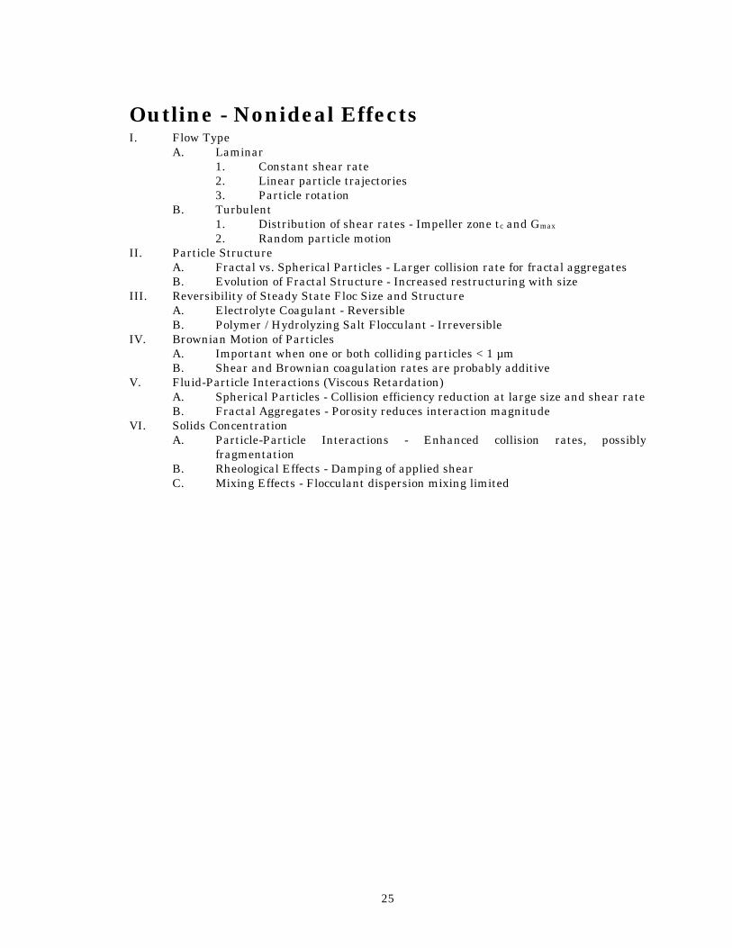
25

Outline - Nonideal Effects I. Flow Type

A. Laminar 1. Constant shear rate 2. Linear particle trajectories 3. Particle rotation

B. Turbulent 1. Distribution of shear rates - Impeller zone tc and Gmax 2. Random particle motion

II. Particle Structure A. Fractal vs. Spherical Particles - Larger collision rate for fractal aggregates B. Evolution of Fractal Structure - Increased restructuring with size

III. Reversibility of Steady State Floc Size and Structure A. Electrolyte Coagulant - Reversible B. Polymer / Hydrolyzing Salt Flocculant - Irreversible

IV. Brownian Motion of Particles A. Important when one or both colliding particles < 1 µm B. Shear and Brownian coagulation rates are probably additive

V. Fluid-Particle Interactions (Viscous Retardation) A. Spherical Particles - Collision efficiency reduction at large size and shear rate B. Fractal Aggregates - Porosity reduces interaction magnitude

VI. Solids Concentration A. Particle-Particle Interactions - Enhanced collision rates, possibly

fragmentation B. Rheological Effects - Damping of applied shear C. Mixing Effects - Flocculant dispersion mixing limited

26

Notation a ellipse axis (cm) aI radius of particle with index i (µm) A Hamaker constant (ergs) b ellipse axis (cm) Cs shielding coefficient (-) d0 primary particle diameter (µm) di particle diameter (µm) dmm mass mean particle diameter (µm) D impeller diameter (cm) Df fractal dimension (-) F fluid drag force (g cm/s2) G spatially averaged shear rate (s-1) i number of particles in an aggregate (-) k0 lacunarity (-) l characteristic length (µm) m breakage rate exponent (-) M mass (g) N impeller rotation rate (s-1) NF dimensionless flow number (-) N0 initial number concentration (# / cm3) Pe Peclet number (-) Re Reynolds number (-) Rc aggregate collision radius (µm) Rg aggregate radius of gyration (µm) RH aggregate hydrodynamic radius (µm) Si particle fragmentation rate (s-1) t time (s) t* time spent colliding (s) T rotation period (s) u fluid velocity (cm/s)

ub critical breakage velocity (cm/s) ur, vf, vi fluid velocity (cm/s)

Greek Letters α collision efficiency (-) β i,j collision frequency (cm3/s) γ laminar shear rate (s-1) ε energy dissipation rate (cm2/s3) εb critical fragmentation energy dissipation rate (cm2/s3) η Kolmogorov microscale (µm) κ permeability (cm2) µ fluid viscosity (g / cm s) ν kinematic viscosity (cm2 / s) ω rotation rate (s-1) ρ density (g/cm3) τ characteristic time (s) ψ collision efficiency (-)

27

ξ Debye shielding ratio (-)

28

References Abrahamson, J., “Collision Rates of Small Particles in a Vigorously Turbulent Fluid,” Chem.

Eng. Sci., 30, 1371-1379 (1975). Adachi, Y., “Dynamic Aspects of Coagulation and Flocculation,” Adv. Colloid Interface Sci.,

56, 1-31 (1995). Adachi, Y. and Ooi, S., “Geometrical Structure of a Floc,” J. Colloid Interface Sci., 135, 374-

384 (1990). Adachi, Y., Stuart, M. A. C., and Fokkink, R., “Kinetics of Turbulent Coagulation Studied by

Means of End-Over-End Rotation,” J. Colloid Interface Sci., 165, 310-317 (1994). Adler, P. M., “Heterocoagulation in Shear Flow,” J. Colloid Interface Sci., 83, 106-115

(1981a). Adler, P. M., “Streamlines in and Around Porous Particles,” J. Colloid Interface Sci., 81, 531-

535 (1981b). Akers, R. J., Rushton, A. G., and Stenhouse, J. I. T., "Floc Breakage: The Dynamic Response

of the Particle Size Distribution in a Flocculated Suspension to a Step Change in Turbulent Energy Dissipation," Chem. Eng. Sci., 42, 787-798 (1987).

Allain, C., Cloitre, M., Parisse, F., “Setting by Cluster Deposition in Aggregating Colloidal Suspensions,” J. Colloid Interface Sci., 178, 411 (1996).

Alonso, M., “Distribution of Nearest Neighbors in Dilute Suspensions of Monodisperse Spheres,” J. Chem. Eng. Japan, 29, 416 (1996).

Alvarez, J, Alvarez, J., and Hernandez, M., “A Population Balance Approach for the Description of Particle Size Distribution in Suspension Polymerization Reactors,” Chem. Eng. Sci., 49, 99-113 (1994).

Amal, R., Coury, J. R., Walsh, W. P., and Waite, T. D., "Structure and Kinetics of Aggregating Haematite," Colloid and Surf., 46, 1-19 (1990a).

Amal, R., Raper, J. A., and Waite, T. D., “Effect of Fulvic Acid Adsorption on the Aggregation Kinetics and Structure of Hematite Particles,” J. Colloid Interface Sci., 151, 244-257 (1992).

Amal, R., Raper, J. A., and Waite, T. D., “Fractal Structure of Hematite Aggregates,” J. Colloid Interface Sci., 140, 158-168 (1990b).

Ballica, R., Ryu, D. D. Y., Powell, R. L., Owen, D., “Rheological Properties of Plant Cell Suspensions,” Biotech. Prog. 8, 413-420 (1992).

Batchelor, G. K., The Theory of Homogeneous Turbulence, Cambridge, (1953). Bensley, C. N. and Hunter, R. J., “The Coagulation of Concentrated Colloidal Dispersions at

Low Electrolyte Concentrations I. Rate of Coagulation and the Onset of Instability,” J. Colloid Interface Sci., 92, 436-447 (1983).

Blatz, P. J. and Tobolsky, A. V., “Note on the Kinetics of Systems Manifesting Simultaneous Polymerization-Depolymerization Phenomena,” J. Phys. Chem., 49, 77-80 (1945).

Blunt, M., “Hydrodynamic Force Distribution on a Fractal Cluster,” Phys. Rev A, 39, 5801-5806 (1989).

Bower, C., Washington, C., Purewal, T. S., “The Use Of Image Analysis To Characterize Aggregates In A Shear Field.,” Colloids Surfaces A, 127, 105 (1997).

Brady, J. F. and Bossis, G., “Stokesian Dynamics,” Ann. Rev. Fluid Mech., 20, 111-157 (1988).

Brakalov, L. B., “A Connection Between the Orthokinetic Coagulation Capture Efficiency of Aggregates and their Maximum Size,” Chem Eng. Sci., 42, 2373-2383 (1987).

Brunk, B. K., Koch, D. L., and Lion, L. W., “Turbulent Coagulation of Particles Smaller than the Kolmogorov Length Scale,” submitted to J. Fluid Mechanics, (1997).

Burban, P., Lick, W., and Lick, J., "The Flocculation of Fine-Grained Sediments in Estuarine Waters," J. Geophys. Res., 94, 8323-8330 (1989).

29

Camp, T. R. and Stein, P. G., "Velocity Gradients and Internal Work in Fluid Motion," J. Boston Soc. Civ. Eng., 30, 219, (1943).

Casson, L. W. and Lawler, D. F., "Flocculation in Turbulent Flow: Measurement and Modeling of Particle Size Distributions," J. AWWA, 82 54-68 (1990).

Chatzi, E. G. and Kiparissides, C., “Steady-State Drop-Size Distributions in High Holdup Fraction Dispersion Systems,” AIChE J., 41, 1640-1652 (1995).

Chellam, S. and Wiesner, M. R., “Fluid Mechanics and Fractal Aggregates,” Wat. Res., 27, 1493-1496 (1993).

Chen, D. and Doi, M., “Simulation of Aggregating Colloids in Shear Flow. II,” J. Chem. Phys., 91, 2656-2663 (1989).

Chen, W., Fisher, R. R., Berg, J. C., "Simulation of Particle Size Distribution in an Aggregation-Breakup Process," Chem. Eng. Sci., 45, 3003-3006 (1990).

Chen, Z.-Y., Meakin, P., Deutch, J. M., “Comment on ‘Hydrodynamic Behavior of Fractal Aggregates’,” Phys. Rev. Lett., 59, 2121 (1987).

Clark, M. M., “Critique of Camp and Stein’s RMS Velocity Gradient,” J. Env. Eng., 111, 741-754 (1985).

Clark, M. M., and Flora, J. R. V., "Floc Restructuring in Varied Turbulent Mixing," J. Colloid and Interface Sci., 147, 407-421 (1991).

Cleasby, J. L., “Is Velocity Gradient a Valid Turbulent Flocculation Parameter?,” J. Env. Eng., 110, 875-897 (1984).

Cohen R. D. and Wiesner, M. R., “Equilibrium Structure and the Kinetics of Fractal Aggregation,” J. Surface Sci. Technol., 6, 25-46 (1990).

Coulaloglou, C. A. and Tavlarides, L. L., “Description of Interaction Processes in Agitated Liquid-Liquid Dispersions,” Chem. Eng. Sci., 32, 1289-1297 (1977).

Curtis, A. S. G. and Hocking, L. M., “Collision Efficiency of Equal Spherical Particles in a Shear Flow,” Trans. Faraday Soc., 66, 1381-1390 (1970).

Cutter, L. A., “Flow and Turbulence in a Stirred Tank,” AIChE J., 12, 35-45 (1966). Danielson, T. J., Muzzio, F. J. and Ottino, J. M., “Aggregation and Structure Formation in

Chaotic and Regular Flows,” Phys. Rev. Lett., 66, 3128-3131 (1991). Davis, R. H. and Hunt, T. P., “Modeling and Measurement of Yeast Flocculation,” Biotech.

Prog. 2, 91-97 (1986). de Boer, G. B. J., Hoedemakers, G. F. M., and Thoenes, D., “Coagulation in Turbulent Flow:

Part I,” Chem. Eng. Res. Des., 67, 301-307 (1989a). de Boer, G. B. J., Hoedemakers, G. F. M., and Thoenes, D., “Coagulation in Turbulent Flow:

Part II,” Chem. Eng. Res. Des., 67, 308-315 (1989b). Delichatsios, M. A. and Probstein, R. F., "Coagulation in Turbulent Flow: Theory and

Experiment," J. Colloid Interface Sci., 51, 394-405 (1975). Delichatsios, M. A., "Particle Coagulation in Steady Turbulent Flows: Application to Smoke

Aging," J. Colloid Interface Sci., 78, 163-174 (1980). Delichatsios, M. A., and Probstein, R. F., "The Effect of Coalescence on the Average Drop Size

in Liquid-Liquid Dispersions," Ind. Eng. Chem., Fund., 15, 134-138 (1976). Dentel, S. K. and Gossett, J. M., "Coagulation of Organic Suspensions with Aluminum Salts,"

Journal Water Pollution Control Federation, 59 101-108 (1987). Dentel, S. K. and Gossett, J. M., "Mechanisms of Coagulation with Aluminum Salts," J.

AWWA, 80 187-198 (1988). Dentel, S. K., "Application of the Precipitation-Charge Neutralization Model of Coagulation,"

Environmental Science & Technology, 22 825-832 (1988). Dentel, S. K., “Coagulant Control in Water Treatment,” Crit. Rev. Env. Control, 21, 41-135

(1991). Dickinson, E., “Kinetic Theory of Coagulation for a Concentrated Dispersion,” J. Colloid

Interface Sci., 98, 587-589 (1984). Dogariu, A., Uozumi, J., and Asakura, T., “Enhancement of the Bacscattered Intensity from

Fractal Aggregates,” Waves Random Media, 2, 259-263 (1992).

30

Doi, M. and Chen, D., “Simulation of Aggregating Colloids in Shear Flow,” J. Chem. Phys., 90, 5271-5279 (1989).

Dukhin, A. S. And Goetz, P. J., “Acoustic and Electroacoustic Spectroscopy,” Langmuir, 12, 4336-4344, (1996).

Eschenazi, E. and Papadopoulos, K. D., “Collision Probabilities in Concentrated Suspensions: Two Dimensional Case,” J. Colloid Interface Sci, 170, 293-294 (1995).

Fair, G. M. and Gemmell, R. S., “A Mathematical Model of Coagulation,” J. Colloid Interface Sci., 19, 360-372 (1964).

Feke, D. L. and Schowalter, W. R., “The Effect of Brownian Diffusion on Shear-Induced Coagulation of Colloidal Dispersions,” J. Fluid Mech., 133, 17-35 (1983).

Finsy, R., “Particle Sizing in the Submicron Range by Dynamic Light Scattering,” Kona, 11, 17-32 (1993).

Ford, T. F., “Viscosity-Concentration and Fluidity-Concentration Relationships for Suspensions of Spherical Particles in Newtonian Liquids,” J. Phys. Chem., 64, 1168-1174 (1960).

Francois, R. J. and Van Haute, A. A., "Floc Strength Measurements Giving Experimental Support for a Four Level Floc Structure," in Chemistry for the Protection of the Environment, Elsevier, Amsterdam, 221 (1984).

Francois, R. J., "Ageing of Aluminum Hydroxide Flocs," Water Res., 21, 523-531 (1987). Francois, R. J., "Strength of Aluminum Hydroxide Flocs," Water Research, 21, 1025-1030

(1987). Friedlander, S. K., Smoke, Dust, and Haze, Wiley, New York, (1977). Gillespie, T., “The Effect of Aggregation and Particle Size Distribution on the Viscosity of

Newtonian Suspensions,” J. Colloid Int. Sci., 94, 166-173 (1983). Glasgow, L. A. and Kim, Y. H., "Characterization of Agitation Intensity in Flocculation

Processes," J. Env. Eng., 112, 1158-1163 (1986). Glasgow, L. A. and Liu, S. X., "Effects of Dosing Regimen and Agitation Profile Upon Floc

Characteristics," Chem. Eng. Commun., 132, 223-237 (1995). Glasgow, L. A. and Luecke, R. H., “Mechanisms of Deaggregation for Clay-Polymer Flocs in

Turbulent Systems,” Ind. Eng. Chem. Fundam., 19, 148-156 (1980). Grabenbauer, G. C. and C. E. Glatz, "Protein Precipitation-Analysis of Particle Size

Distribution and Kinetics," Chem. Eng. Comm., 12, 203-219 (1981). Greene, M. R., Hammer, D. A., and Olbricht, W. L., “The Effect of Hydrodynamic Flow Field

on Colloidal Stability,” J. Colloid Interface Sci., 167, 232-246 (1994). Gregory, J. And Gubai, L., “Effects of Dosing and Mixing Conditions on Polymer Flocculation

of Concentrated Suspensions,” Chem. Eng. Comm., 108, 3-21 (1991). Gregory, J., “Effect of Dosing and Mixing Conditions on Flocculation by Polymers,” in

Advances in Measurement and Control of Colloidal Processes, R. A. Williams and N. C. de Jaeger, eds., Butterworth-Heinemann, Oxford, (1991).

Gruy, F. and Saint-Raymond, H., “Turbulent Coagulation Efficiency,” J. Colloid Interface Sci., 185, 281- (1997).

Guibai, L. and Gregory, J., "Flocculation and Sedimentation of High-Turbidity Waters," Water Research, 25, 1137-1143 (1991).

Han, M. and Lawler, D. F., "The (Relative) Insignificance of G in Flocculation," J. AWWA, 79-91 (1992).

Hansen, S. and Ottino, J. M., “Agglomerate Erosion: A Non-Scaling Solution to the Fragmentation Equation,” Phys. Rev. E, 53, 4209-4212 (1996).

Hansen, S. and Ottino, J. M., “Aggregation and Cluster Size Evolution in Non-Homogeneous Flows,” J. Colloid Interface Sci., 179, 89-103 (1996).

Heffels, C., Willemse, A., Scarlett, B., “Possibilies of Near Backward Light Scattering for Characterizing Dense Particle Systems,” Powder Tech., 86, 127-135 (1996).

31

Higashitani, K., Yamauchi, K., Matsuno, Y., and Hosokawa, G., "Kinetic Theory of Shear Coagulation for Particles in a Viscous Fluid," J. Chem. Eng. Japan, 15, 299-304 (1982).

Higashitani, K., Yamauchi, K., Matsuno, Y., and Hosokawa, G., "Turbulent Coagulation of Particles Dispersed in a Viscous Fluid," J. Chem. Eng. Japan, 16, 299-304 (1983).

Horwatt, S. W., Feke, D. L., amd Manas-Zloczower, I., “The Influence of Structural Heterogeneities on the Cohesivity and Breakup of Agglomerates in Simple Shear Flow,” Powder Tech., 72, 113-119 (1992).

Hunter, R. J., Introduction to Modern Colloid Science, Vol. 1, Oxford Science Publications, New York, (1993).

Jeffery, G. B., “The Motion of Ellipsoid Particles Immersed in a Viscous Fluid,” Proc. Roy. Soc. London, A102, 161-179 (1922).

Jiang and Logan, B. E., “Fractal Dimensions of Aggregates Determined from Steady State Size Distributions,” Env. Sci. and Tech., 25, 2031-2038 (1991).

Johnson, C. P., Li, X., and Logan, B. E., “Settling Velocities of Fractal Aggregates,” Env. Sci. Tech., 30, 1911-1918 (1996).

Jullien, R. and Meakin, P., “Simple Models for the Restructuring of Three-Dimensional Ballistic Aggregates,” J. Colloid Interface Sci., 127, 265-272 (1989).

Jung, S.J., Amal, R., and Raper, J.A., “Monitoring effects of shearing on floc structure using small-angle light scattering,” Powder Tech., 88, 51 (1996).

Jung, S.J., Amal, R., Raper, J.A., “The Use of Small Angle Light Scattering to Study Structure of Flocs,” Particle & particle systems characterization, 12, 274 (1995).

Kim, Y. H. and Glasgow, L. A., "Simulation of Aggregate Growth and Breakage in Stirred Tanks," Industrial & Engineering Chemistry Research, 26 1604-1609 (1987).

Koh, P. T. L., Andrews, J. R. G., and Uhlerr, P. H. T., "Flocculation in Stirred Tanks," Chem. Eng. Sci., 39, 975-985 (1987).

Koh, P. T. L., Andrews, J. R. G., and Uhlerr, P. H. T., "Modelling Shear Flocculation by Population Balances," Chem. Eng. Sci., 42, 353-362 (1984).

Kruis, F. E. and Kusters, K. A., “The Collision Rate of Particles in Turbulent Flow,” Chem. Eng. Comm., 158, 201-230 (1997).

Krutzer, L. L. M., Van Diemen, A. J. G., and Stein, H. N., “The Influence of the Type of Flow on the Orthokinetic Coagulation Rate,” J. Colloid Interface Sci., 171, 429-438 (1995).

Kusters, K. A., "The Influence of Turbulence on Aggregation of Small Particles in Agitated Vessels," Ph. D. Thesis, Eindhoven University of Technology, The Netherlands, (1991).

Kusters, K. A., Wijers, J. G., and Thoenes, D., “Aggregation Kinetics of Small Particles in Agitated Vessels,” Chem. Eng. Sci., 52, 107-121 (1996).

Lamb, H., Hydrodynamics, Dover, New York (1943). Lawler, D. F., “Physical Aspects of Flocculation: from Microscale to Macroscale,” Wat. Sci.

Tech., 27, 165-180 (1993). Leu, R. and Ghosh, M. M., "Polyelectrolyte Characteristics and Flocculation," J. AWWA, 80,

159-167 (1988). Levenspiel, O., Chemical Reactor Engineering, Wiley, New York (1972). Levich, V. G., "Physicochemical Hydrodynamics," Prentice Hall, New York, (1962). Lilge, D. And Horn, D., “Diffusion in Concentrated Dispersions: A Study with Fiber-Optic

Quasi-Elastic Light Scattering (FOQELS),” Colloid Polymer Sci., 269, 704-712 (1991).

Macosko, C. W., “Shear Rheometry: Drag Flows,” in Rheology Principles, Measurements, and Applications, C. W. Macosko, ed., VCH Publishers, New York, 188-205 (1994).

Mandelbrot, B. B., Passoja, D. E., and Paullay, A. J., “Fractal Character of Fracture Surfaces of Metals,” Nature, 308, 721-722 (1984).

Mandelbrot, B. B., The Fractal Geometry of Nature, W. H. Freeman and Company, New York, (1987).

32

Manley, R. J. and Mason, S. G., “Particle Motions in Sheared Suspensions. III. Further Observations on Collisions of Spheres,” Can. J. Chem., 33, 736-773 (1955).

McClements, D. J. and Coupland, J. N., “Theory of Droplet Size Distribution Measurements using Ultrasonic Spectroscopy,” Colloids Surfaces, 117, 161-170 (1996).

Meakin, P., "Fractal Aggregates," Adv. Colloid Interface Sci., 28, 249-331 (1988). Mewis, J. and Macosko, C. W., “Suspension Rheology,” in Rheology Principles, Measurements,

and Applications, C. W. Macosko, ed., VCH Publishers, New York, 425-474 (1994). Mills, P. D. A., Goodwin, J. W., and Grover, B. W., “Shear Field Modification of Strongly

Flocculated Suspensions - Aggregate Morphology,” Colloid Polymer Sci., 269, 949-963 (1991).

Monnier, O., Klein, J.-P., Ratsimba, B., “Particle Size Determination by Laser Reflection: Methodology and Problems,” Part. Part. Sys. Char., 13, 10 (1996).

Muzzio, F. J. and Ottino, J. M., “Coagulation in Chaotic Flows,” Phys. Rev. A, 38, 2516-2524 (1988).

Neimark, A. V., Koylu, U. O., and Rosner, D. E., “Extended Characterization of Combustion-Generated Aggregates: Self-Affinity and Lacunarities,” J. Colloid Interface Sci., 180, 590 (1996).

Ødegaard, H., "Orthokinetic Flocculation of Phosphate Precipitates in a Multicomponent Reactor with Non-Ideal Flow," Prog. Wat. Tech., Suppl. 1, 61-88 (1979).

Oles, V., "Shear-Induced Aggregation and Breakup of Polystyrene Latex Particles," J. Colloid Interface Sci., 154, 351-358 (1992).

Pandya, J. D. and Spielman, L. A., "Floc Breakage in Agitated Suspensions: Theory and Data Processing Strategy," J. Colloid Interface Sci., 90, 517-531 (1982).

Parker, D. S., Kaufman, W. J., and Jenkins, D., "Floc Breakup in Turbulent Flocculation Processes," J. San. Eng. Div., Proc. ASCE, 98, 79-99 (1972).

Peng, S. J. and Williams, R. A., “Direct Measurement of Floc Breakage in Flowing Suspensions,” J. Colloid Interface Sci., 166, 321-332 (1994).

Potanin, A. A. and Uriev, N. B., “Microrheological Models of Aggregated Suspensions in Shear Flow,” J. Colloid Int. Sci., 142, 385-395 (1991).

Potanin, A. A., “On the Computer Simulation of the Deformation and Breakup of Colloidal Aggregates in Shear Flow,” J. Colloid Int. Sci., 145, 140-157 (1991).

Potanin, A. A., “On the Computer Simulation of the Deformation and Breakup of Colloidal Aggregates in Shear Flow,” J. Colloid Interface Sci., 157, 399-410 (1993).

Potanin, A. A., “On the Mechanism of Aggregation in the Shear Flow of Suspensions,” J. Colloid Interface Sci., 145, 140-157 (1991).

Pusey, P. N., Rarity, J. G., Klein, R., Weitz, D. A., “Comment on ‘Hydrodynamic Behavior of Fractal Aggregates’,” Phys. Rev. Lett., 59, 2122 (1987).

Reich, I. and Vold, R. D., "Flocculation-Deflocculation in Agitated Suspensions. I. Carbon and Ferric Oxide in Water," J. Phys. Chem., 63, 1497-1501 (1959).

Reuβ, M., Josic, D., Popovic, M., and Bronn, W. K., “Viscosity of Yeast Suspensions,” Eur. J. Appl. Microbiology Bitoech., 8, 167-175 (1979).

Roels, J. A., Van den Berg, J., Voncken, R. M., “The Rheology of Mycelial Broths,” Biotech. Bioeng., 31, 19-23 (1988).

Rogak, S. N. and Flagan, R. C., “Stokes Drag on Self-Similar Clusters of Spheres,” J. Colloid Interface Sci., 134, 206-218 (1990).

Saffman, P., and Turner, J., "On the Collision of Drops in Turbulent Clouds," J. Fluid Mech., 1, 16-30 (1956).

Scragg, A. H., Allen, E. J., Bond, P. A., Snart, N. J., “Rheological Properties of Plant Cell Suspension Cultures,” in Secondary Metabolism in Plant Cell Cultures, P. Morris, A. H. Scragg, A. Stafford, and M. W. Fowler, eds., Cambridge University Press, Cambridge, England (1986).

Seckler, M. M., Bruinsma, O. S. L., and Van Rosmalen, G. M., “Influence of Hydrodynamics on Precipitation: A Computational Study,” Chem. Eng. Comm., 135, 113-131 (1995).

33

Shamlou, P. A. and Tichener-Hooker, N., “Turbulent Aggregation and Breakup of Particles in Liquids in Stirred Vessels,” in Processing of Solid-Liquid Suspensions, P. A. Shamlou, ed., Butterworth Heinemann, Oxford, 1-25 (1993).

Shimmons, B. W., Svreck, J. P., Zajie, J. E., “Cell Concentration Control by Viscosity,” Biotech. Bioeng., 18, 1793-1805 (1976).

Shinnar, R., “On the Behavior of Liquid Dispersion in Mixing Vessels,” J. Fluid Mech., 10, 259-275 (1961).

Smit, D. J., Paterson, W. R., and Hounslow, M. J., “Aggregation and Gelation - II. Mixing Effects in Continuous Flow Vessels,” Chem. Eng. Sci., 49, 3147-3167 (1994).

Smoluchowski, M., “Versuch Einer Mathematischen Theorie de Koagulations- Kinetic Kolloider Losungen,” Z. Phys. Chem., 92, 129 (1917).

Sonntag, R. C. and Russel, W. B., "Structure and Breakup of Flocs Subjected to Fluid Stresses I. Shear Experiments," J. Colloid Interface Sci., 113, 399-413 (1986).

Sonntag, R. C. and Russel, W. B., "Structure and Breakup of Flocs Subjected to Fluid Stresses II. Theory," J. Colloid Interface Sci., 115, 378-389 (1987).

Spicer, P. T. and Pratsinis, S. E., “Coagulation-Fragmentation: Universal Steady State Particle Size Distributions,” AIChE J., 42, 1612-1620 (1996).

Spicer, P. T. and Pratsinis, S. E., “Shear-Induced Flocculation: The Evolution of Floc Structure and the Shape of the Size Distribution at Steady State,” Wat. Res., 30, 1049-1056 (1996).

Spicer, P. T., Keller, W., and Pratsinis, S. E., “The Effect of Impeller Type on Floc Size and Structure during Shear-Induced Flocculation,” J. Colloid Interface Sci., 184, 112-122 (1996).

Spielman, L. A., "Hydrodynamic Aspects of Flocculation," in The Scientific Basis of Flocculation, Ives, K. J., ed., Sijthoff and Noordhoff, The Netherlands, 207-233 (1978).

Spielman, L. A., “Viscous Interactions in Brownian Coagulation,” J. Colloid Interface Sci., 33, 562-571 (1970).

Stewart, R. F. and Sutton, D., “Characterisation of the Structure of Concentrated, Flocculated Suspensions, Part. Sci. Tech., 4, 251-263 (1986).

Stewart, R. F. and Sutton, D., “Control of Structure in Particulate Solids Suspensions,” in Solid-Liquid Separation, J. Gregory, ed., Ellis Horwood Ltd., Chichester, 111-129 (1984).

Swift, D. L., and Friedlander, S. K., "The Coagulation of Hydrosols by Brownian Motion and Laminar Shear Flow," J. Colloid Interface Sci., 19, 621-647 (1964).

Tambo, N. and Watanabe, Y., "Physical Aspect of Flocculation Process: I. Fundamental Treatise," Water Res., 13, 429-439 (1979).

Tambo, N., "Basic Concepts and Innovative Turn of Coagulation/Flocculation," Water Supply, 9, 1-10 (1991).

Tanaka, H., “Oxygen Transfer in Broths of Plant Cells at High Density,” Biotech. Bioeng., 24, 424-442 (1982).

Thomas, D. G., “Transport Characteristics of Suspension: VIII. A Note on the Viscosity of Newtonian Suspensions of Uniform Spherical Particles,” J. Colloid Int. Sci., 20, 267-327 (1965).

Thomas, D. G., “Turbulent Disruption of Flocs in Small Particle Size Suspensions,” AIChE J., 10, 517-523 (1964).

Tomi, D. T. and Bagster, D. F., “The Behaviour of Aggregates in Stirred Vessels, Part 1-Theoretical Considerations on the Effects of Agitation,” Trans. Inst. Chem. Eng., 56, 1-8 (1978).

Torres, F. E., Russel, W. B., and Schowalter, W. R., “Simulations of Coagulation in Viscous Flows,” J. Colloid Interface Sci., 145, 51-73 (1991b).

34

Torres, F. E., Russel, W. R., and Schowalter, W. R., "Floc Structure and Growth Kinetics for Rapid Shear Coagulation of Polystyrene Colloids," J. Colloid Interface Sci., 142, 554-574 (1991a).

Trevelyan, B. J. and Mason, S. G., “Particle Motion in Sheared Suspensions. I. Rotations,” J. Colloid Interface Sci., 6, 354-367 (1951).

Uriev, N.B. and Ladyzhinsky, I.Y., “Fractal models in rheology of colloidal gels,” Colloids Surfaces A, 108, 1 (1996).

van de Ven, T. G. M. and Mason, S. G., “The Microrheology of Colloidal Dispersions VII. Orthokinetic Doublet Formation of Spheres,” Colloid Polymer Sci., 255, 468-479 (1977a).

van de Ven, T. G. M. and Mason, S. G., “The Microrheology of Colloidal Dispersions VIII. Effect of Shear on Perikinetic Doublet Formation,” Colloid Polymer Sci., 255, 794-804 (1977b).

van de Ven, T. G. M., Colloidal Hydrodynamics, Academic Press, New York (1989). van Saarloos, W., “On the Hydrodynamic Radius of Fractal Aggregates,” Physica, 147A, 280-

296 (1987). Vand, V., “Viscosity of Solutions and Suspensions. I Theory,” J. Phys. Chem., 52, 277-299

(1948). Veerapaneni, S. and Wiesner, M. R., “Hydrodynamics of Fractal Aggregates with Radially

Varying Permeability,” J. Colloid Interface Sci., 177, 45-57 (1996). Vold, M. J., “Computer Simulation of Floc Formation in a Colloidal Suspension,” J. Colloid

Sci., 18, 684-695 (1963). Wang, D. G., Sadhal, S. S., and Campbell, C. S., “Particle Rotation as a Heat Transfer

Mechanism,” Int. J. Heat Mass Trans., 32, 1413-1423 (1989). Warren, L. J., “Shear-Flocculation of Ultrafine Scheelite in Sodium Oleate Solutions,” J.

Colloid Interface Sci., 50, 307-218 (1975). Wiersma, D. And Lagendijk, A., “Laser Action in Very White Paint,” Physics World, January,

33-37 (1997). Wiesner, M. R., "Kinetics of Aggregate Formation in Rapid Mix," Water Res., 26, 379-387

(1992). Williams, R. A., Peng, S. J., and Naylor, A., “In situ Measurement of Particle Aggregation

and Breakage Kinetics in a Concentrated Suspension,” Powder Tech., 73, 75-83 (1992).

Wiltzius, P., “Hydrodynamic Behavior of Fractal Aggregates,” Phys. Rev. Lett., 58, 710-713 (1987).

Wolynes, P. G. and McCammon, J. A., “Hydrodynamic Effect on the Coagulation of Porous Biopolymers,” Macromolecules, 10, 86-87 (1977).

Ye, J. and Roco, M., “Particle Rotation in a Couette Flow,” Phys. Fluids A, 4, 220-224 (1992). Yoshimura, A. S. and Prud’homme, R. K., “Response of an Elastic Bingham Fluid to

Oscillatory Shear,” Rheol. Acta, 26, 428-436 (1987). Zeichner, G. R. and Schowalter, W. R., “Effects of Hydrodynamic and Colloidal Forces on the

Coagulation of Dispersions,” J. Colloid Interface Sci., 71, 237-253 (1979). Zeichner, G. R. and Schowalter, W. R., “Use of Trajectory Analysis to Study Stability of

Colloidal Dispersions in Flow Fields,” AIChE J., 23, 243-253 (1977). Zhong, J.-J., Seki, T., Kinoshita, S.-I., Yoshida, T., “Rheological Characteristics of Cell

Suspension and Cell Culture of Perilla frutescens,” Biotech. Bioeng., 40, 1256-1262 (1992).

35

Chapter 2 - Time Lag for Steady State Attainment

The dynamic behavior and the attainment of steady state by a flocculating suspension in a stirred tank are evaluated using a population balance model. At long times, shear-induced coagulation and fragmentation reach a steady state, resulting in a particle size distribution (PSD) that is invariant (self-preserving) with respect to shear. The geometric standard deviations, σg, of the self-preserving number or volume PSDs are 2.22 or 1.79, respectively, for the employed coagulation and fragmentation rates of flocculation. The time required to reach a steady state PSD (time lag) is determined as a function of a dimensionless group comprised of the relative rates of coagulation and fragmentation. The effect of the omnipresent variable shear rate in stirred tanks during shear-induced flocculation is investigated through a sinusoidal function of the spatially averaged velocity gradient. Increasing the amplitude of the shear rate fluctuation decreases the steady state mass mean floc size, the maximum σg, and the time lag for attainment of steady state. The asymptotic (self-preserving) σg is not affected by the shear rate amplitude provided that >99% of the primary particles have grown to larger sizes. This chapter has been published: Spicer, P. T., Pratsinis, S. E., Trennepohl, M. D. and Meesters, G. H. M., "Coagulation and Fragmentation: The Variation of Shear Rate and the Time Lag for Attainment of Steady State," Ind. Eng. Chem. Res., 35, 3074-3080 (1996).

36

Introduction An important design and control parameter in flocculation processes is the size distribution of the suspended particles. In most practical systems, a steady state or equilibrium is reached between coagulation and fragmentation after a certain time (time lag) and the particle size distribution (PSD) no longer changes. This time lag determines the process requirements (i.e. batch time, power input, etc.) of a flocculation process. Experimental studies have shown that the spatially averaged shear rate varies significantly throughout a stirred tank (Cutter, 1966; Sprow, 1967). Realistic descriptions of flocculation account for the high shear region around the impeller (impeller zone) and various bulk regions above and below the impeller with significantly lower relative shear rates. Koh et al. (1984; 1987) for example, coupled multi-compartmental models of a stirred tank with the population balance equations to fit data on scheelite flocculation but considered only coagulation with no fragmentation. A two-compartment model gave results as good as models using a larger number of compartments. Kim and Glasgow (1987) developed a Monte Carlo model of coagulation and fragmentation assuming random movement / shearing of particles, a size-dependent fragmentation rate, and a time step based on the frequency of exposure to the impeller zone. Few comparisons with experimental data were performed, and good agreement with the evolution of the average size of kaolin-polymer flocs was reported (Kim and Glasgow, 1987). Kusters (1991) combined a six-compartment stirred tank model with analytical velocity profiles to track particle residence times in each compartment. He derived expressions for the frequency of successful coagulation and fragmentation and predicted the evolution of the average floc size well. Recently, Seckler et al. (1995) studied stirred tank hydrodynamics using computational fluid dynamic (CFD) models coupled with a moment model of the particle size distribution during precipitation. The model identified specific regions of particle formation in a precipitation reactor. The shape of the asymptotic PSD affects the efficiency of a solids removal process. Theoretical investigations have indicated that pure shear-induced coagulation does not result in a self-preserving PSD (Swift and Friedlander, 1964; Pulvermacker and Ruckenstein, 1974), that is, a PSD whose shape scales with the average particle size. Theoretical (Tambo and Watanabe, 1979; Family et al., 1986; Meakin, 1988; Cohen, 1992; Spicer and Pratsinis, 1996a) and experimental (Spicer and Pratsinis, 1996b) studies have shown, however, that the steady state PSD from coagulation-fragmentation processes is self-preserving with respect to process conditions. When self-similarity is observed, the individual coagulation and fragmentation rates in the suspension may be determined by deconvolution of the steady state PSD (Narsimhan et al., 1980; Wright and Ramkrishna, 1994). The time lag for attainment of steady state by a coagulation-fragmentation process has been investigated previously (Blatz and Tobolsky, 1945; Peled et al., 1995) but models incorporating realistic, size-dependent rate expressions have not been used. In addition, few studies have been carried out on the effect of heterogeneous flow conditions on a flocculating particle size distribution. The objective of this study is to determine the time lag for attainment of steady state by coagulation and fragmentation using rates commonly encountered during flocculation (Lu and Spielman, 1985). To meet this goal a population balance model is used (Spicer and Pratsinis, 1996a) that has successfully simulated experimental data of polystyrene particle flocculation (Oles, 1992). Furthermore, the effect of constant and varying shear rates on the time lag and the polydispersity of the steady state PSD is investigated and related to controllable process variables through dimensionless groups.

37

Theory The dynamic behavior of the particle size distribution undergoing simultaneous coagulation and fragmentation is given by (Friedlander, 1977; Kusters et al., 1993):

dndt

=12

(u ,u )n n - n (u ,u )n - S n + S ni

j+k=ij k j k i

k=1

max

k i k i ij=i

max

j j∑ ∑ ∑αβ αβ γ i j, (2-1)

where ni is the number concentration of flocs of size i (meaning that a single floc contains i primary particles). The first term on the right hand side (RHS) of Equation (2-1) represents the formation of particles comprised of i primary particles by collisions of smaller j- and k-sized particles. The second RHS term denotes the loss of particles of size i by collision with particles of any other size. The third RHS term describes the loss of particles of size i by fragmentation and the fourth RHS term describes the formation of particles of size i by the fragmentation of larger particles. The index max represents the largest particle size. Equation (2-1) is the discrete form of the population balance equation, that is, it describes the change in number concentration of each individual particle size. Thus, in order to model the evolution of the detailed particle size distribution during flocculation, the solution of an enormous number of differential equations would be required using a discrete model. To ease computations, the particle size distribution is divided into size classes or sections. Equations are written describing the change in particle number concentration in each section based on Hounslow et al. (1988) and Spicer and Pratsinis (1996a):

i

j=1

i-2j-i+1

i-1, j i 1 j i-1,i-1 i-12

ij=1

i-1j-i

i, j j

ij=i

i max

i, j j i i i, j j jj i

i max

dNdt

= 2 N N +12

N - N 2 N

- N N - S N + S N

∑ ∑

∑ ∑

−

=

α β α β α β

α β Γ

(2-2)

where Ni is the number concentration of flocs of size class i (meaning that a single floc contains 1.5*2i-1 primary particles), α is the collision efficiency for coagulation, βi,k is the collision frequency for particles of size class i and k with characteristic volumes vi and vk, Si is the fragmentation rate of flocs of volume vi, and Γi,j is the breakage distribution function defining the volume fraction of the fragments of size i coming from j-sized particles. The index i max is the number of sections used in the model (here i max = 30). The collision frequency for turbulent shear-induced coagulation, in the absence of viscous retardation and floc structural effects, is given by (Saffman and Turner, 1956):

( )βενi j i ja a, .=

+1294

1

2 3 (2-3)

and the spatially averaged shear rate (Clark, 1985) given for fluctuating shear rates by:

G G t= +' sin( )ω (2-4)

G’ is a constant (e.g. 50 s-1) and ω is the maximum magnitude of the fluctuation in G. A range of ω was examined here (ω = 0, 30, 40, 50 s-1). The fragmentation rate is a function of particle volume (Pandya and Spielman, 1982):

S = Avi ia (2-5)

where a = 1/3 (Boadway, 1978; Peng and Williams, 1994), consistent with the theoretical expectation that breakage rate is proportional to the floc diameter. The parameter A is the breakage rate coefficient for shear-induced fragmentation (Pandya and Spielman, 1982):

38

A A G y= ' (2-6)

where y is a constant inversely proportional to the floc strength and A’ is a proportionality constant that is determined experimentally. The value of y = 1.6 was used in all calculations corresponding to kaolin - polymer and polystyrene flocs (Pandya and Spielman, 1982; Spicer and Pratsinis, 1996a). The constant A’ affects the relative strength of fragmentation relative to coagulation and a value of 0.0047 is used here (Oles, 1992; Spicer and Pratsinis, 1996a). For all calculations, binary breakage was assumed (Spicer and Pratsinis, 1996a):

, for j= i +1

otherwise

Γi, j

=0,

=v

vj

i (2-7)

Equations (2-3)-(2-7) were substituted into Equation (2-2) and the sectional model was solved numerically using DGEAR, an ordinary differential equation solver (IMSL, 1989). The behavior of a coagulation-fragmentation system is a function of the relative significance of the rates of coagulation and fragmentation (Blatz and Tobolsky, 1945). As a result, it is convenient to define a dimensionless group that characterizes the relative significance of coagulation versus fragmentation, CF:

CFS v

= 0 0

0 0φβ ,

(2-8)

where φ is the volume fraction of suspended particles, v0 is the volume of a primary particle and β0,0 and S0 are obtained by substituting v0 into Equations (2-3) and (2-5), respectively.

Results and Discussion Unless stated otherwise, all calculations were carried out for G = 50 s-1, α = 1, ω = 0, A’ = 0.0047, y = 1.6, initial diameter d0 = 2.17 µm (corresponding to an initial volume of v0 = 5.35 µm3), and initial number concentration N1 = 9.3 x 106 cm-3 (Oles, 1992; Spicer and Pratsinis, 1996a). The model was validated by comparison with analytical solutions for the case of pure coagulation with a size-dependent kernel (Golovin, 1963), pure fragmentation (Williams, 1990), and the combined case (Blatz and Tobolsky, 1945). At all conditions excellent agreement between the numerical and analytical solutions was obtained (Spicer and Pratsinis, 1996a).

Development of the Steady State Floc Size Distribution Figure 2-1 shows the evolution of the initially monodisperse particle size distribution as a function of dimensionless time, τ = Gφt (Oles, 1992). Initially, growth is slow as the small primary particles collide and form larger ones. Figure 2-1 shows the evolution of the number distribution. After 1τ, the distribution remains in the first few size classes. After 10τ, an additional, bell-shaped mode forms and the primary particle size class is further depleted. Fragmentation prevents further growth of the larger mode and these particles serve as collectors of fines (primaries), accelerating the depletion of the primary particles until after 20τ the distribution no longer changes (e.g. at 30τ). It is worth noting that the primary particles constitute a large (number) fraction, N1ss = 5%, of the steady state size distribution. Figure 2-1b shows the evolution of the volume distribution as a function of τ. Similar to Figure 2-1a, the initially monodisperse distribution grows into the larger size sections,

39

forming a bell-shaped mode after 1τ. After 10τ, the distribution is indistinguishable from that at 15τ and steady state is attained in about half the time required for the number-based distribution. The steady state volume-based PSD is attained much faster than the number-based distribution because the primary particles do not contribute significantly to the former PSD.

Effect of Shear Rate on the Attainment of Steady State The geometric standard deviation of the floc size distribution, σg, quantitatively characterizes the width of the distribution (Hinds, 1982). Figure 2-2 shows the evolution of σg for various shear rates, G (ω = 0). After an initial lag period the number-based geometric standard deviation, σgn, increases as the distribution broadens into the larger size classes (Figure 2-1a). A maximum value is reached (e.g. σg = 3.27 at τ = 15 for G = 10 s-1) corresponding to the maximum displacement of the larger mode from the primary particle mode of the distribution. As the primary particles are depleted (Figure 2-1a), the σgn decreases until leveling off at an asymptotic value, σgnss, corresponding to the attainment of the steady state size distribution (σgnss = 2.22 at τ = 28 for G = 10 s-1). Increasing the shear rate, G, results in an increased fragmentation rate (Equation (2-6)) preventing further growth of the steady state particle size distribution. As a result, the steady state PSD is displaced to smaller sizes and narrowed as the number of primary particles present at steady state is increased compared to the steady state PSD at lower shear rates (e.g. at G = 50 s-1 the concentration of primary particles at steady state is N1ss = 5 %). This is shown in Figure 2-2 where the σgnss decreases with increasing G. Furthermore, the maximum in σgn decreases with increasing G since the two size modes (primary particles and flocs) become increasingly indistinguishable. For example, the primary particle concentration at steady state is 5 % for G = 50 s-1 and becomes 18 % for G = 100 s-1 (Spicer and Pratsinis, 1996a). Figure 2-2 also shows the evolution of the geometric standard deviation, σgv, of the corresponding volume-based PSD. A rapid increase in σgv is initially observed as the distribution broadens and larger particles are formed (Figure 2-1b). As with the number-based PSD, a maximum is reached, corresponding to the maximum separation of the primary particle and floc modes. At a constant G, the maximum σgv is smaller than the maximum σgn because of the larger relative contribution of the primary particles to the number- versus the volume-based PSD. At the employed shear rates the primary particles contribute little to the latter distribution so the same σgv is attained at all shear rates. The steady state σgv is unchanged by the shear rate, consistent with Spicer and Pratsinis (1996b), who found that shear does not change the width of the polystyrene floc size distribution at steady state so it is self-preserving with respect to shear. Figure 2-3 shows the steady state geometric standard deviation for the number and volume PSD (σgnss and σgvss respectively) as a function of the coagulation-fragmentation group, CF, for various shear rates G and breakup coefficients A. In Figure 2-3, all values of σgnss and σgvss collapse onto a single curve when scaled by the dimensionless parameter CF. This indicates that a universal asymptotic behavior is exhibited by a coagulation-fragmentation system for this combination of rate expressions. In Figure 2-3, the σgnss increases and approaches an asymptotic value of 2.22 with decreasing values of CF. This asymptotic behavior is indicative of the self-preserving properties of the fully developed steady state PSD (Spicer and Pratsinis, 1996a and b). Increasing the CF corresponds to increased fragmentation relative to coagulation, causing σgnss to decrease from its value when fully-developed (N1ss ≤ 0.01 NTss, where NTss is the total number concentration present at steady state). This is attributed to the narrowing of the size distribution as increased fragmentation shifts the distribution to the smallest sections. The threshold CF (1 % from the asymptotic CF) corresponding to N1ss ≤ 0.01 NT is CF = 0.013. Figure 2-3 also shows the

40

effect of CF on σgvss. Here also, increasing CF slightly decreases the σgvss below the self-preserving σgvss = 1.79. The effect of increased fragmentation rates is smaller for the volume- than for the number-based PSD because of the sensitivity of the latter distribution to the dynamics of the primary particles. This is seen in Figure 2-3 as a significant decrease in σgnss to the right of the dotted line indicating the number fraction of the smallest particles exceeding 1 %. For the volume distribution, the deviation of σgvss from self-similarity occurs when V1ss ≥ 0.01 VTss (where VTss is the total solids volume present at steady state). The dynamics of the floc size distribution can be quantitatively characterized through the evolution of the σgn and σgv of the distribution (Figure 2-2). In addition, the σg is readily measured by light-scattering techniques and is used as a measure of product particle quality in numerous industrial processes. Thus, the σg provides a practical and theoretical criterion for the attainment of steady state and thus the time lag before attainment of steady state. By analogy with previous work on Brownian coagulation (Vemury et al., 1994), the criterion for the attainment of steady state was defined as the dimensionless time (τss) at which the distribution was within 1% of its steady state σg. Figure 2-4 shows the steady state time lag, τss, for the number (τnss) and volume (τvss) distributions as a function of CF. As in Figure 2-3, the τss values collapse onto a single curve for the number- and volume-based PSD when scaled with CF. Linear regression gives:

ττ

nss

vss

22.35log 20.69

5.60log 0.496

= − −= − +

CF

CF (2-9)

At low CF, a large difference between the τnss and τvss is observed. Lower values of CF correspond to increased collision rates for small particles (Equation (2-8)). As a result, the size distribution is able to develop into larger sizes before fragmentation halts its progress. Increasing the CF decreases the τss for both number and volume distributions as a result of the increased fragmentation rates and the resulting decreased extent of PSD development. It is interesting to note that the scaling of τss is unchanged by a deviation from the self-preserving σg of the steady state size distribution (i.e. the values of τss collapse onto a single curve even to the right of the broken line indicating the point of deviation from the self-preserving size distribution). The τnss is significantly larger than the τvss as a result of the larger effect of the primary particle dynamics on steady state attainment by the number-based PSD.

Effect of Shear Rate Fluctuations on Steady State Attainment Equation (2-4) is a simplified description of the variation of the instantaneous shear rate within the turbulent flow field of the stirred tank. This description is based on the concept of an average circulation time for a suspended particle or fluid element (Oldshue, 1984; Kim and Glasgow, 1987). Particles are exposed to a spectrum of shear rates during the flocculation process. For example, fluid elements start from a region of say, average G, reach the region of maximum G at the impeller zone, and then reach the relatively stagnant region above the impeller, and finally return back to the high shear impeller zone. This is consistent with the flow pattern for a radial flow impeller such as a Rushton configuration (Holland and Chapman, 1966). Increasing the amplitude of the shear rate fluctuation, ω, increases the range of G experienced by the suspended particles. The shear rate variation for the four cases examined in this study were: G = 50 s-1 and ω = 0, 30, 40, 50 s-1. Figure 2-5 shows the evolution of the dimensionless mass mean floc diameter (Hinds, 1982), dmm / d0 at various shear rate amplitudes. During the growth-dominated region of flocculation, the dmm increases rapidly as shear-induced collisions promote particle growth. As larger particles are formed, the significance of fragmentation increases, the particle

41

growth rate slows down and dmm levels off so a steady state is reached (τ = 8 at ω = 0 as in Figure 2-1 - Figure 2-3). It is interesting to note that the system reaches a stable steady state (with small oscillations) despite the large variance in the value of G, consistent with experimental data (Reich and Vold, 1959; Oles, 1992; Spicer and Pratsinis, 1996b). Increasing the ω slows the growth of dmm, resulting in smaller particles at steady state. The exposure of the flocs to larger shear rates at higher G amplitudes increases their fragmentation rate, providing a greater contribution of fragmentation to the attainment of steady state. During the later stages of flocculation the role of fragmentation in steady state attainment is significant, so the largest values of G restrict floc growth. Figure 2-5 showed that the evolution of the PSD and the average floc size are influenced by fluctuations in the shear rate. Figure 2-6 shows the effect of ω on the evolution of σg for G = 50 s-1. In Figure 2-6, the σgn follows the trend observed in Figure 2-2: the distribution width increases initially, reaches a maximum, then descends to its steady state value. Increasing the ω slightly accelerates the initial (τ < 10) increase in σgn relative to the case of constant shear as a result of the strong dependence of the collision frequency of the larger particles on shear rate (Equation (2-3)). The second mode of the distribution forms more rapidly with increasing shear rate amplitude, thus accelerating the rate of increase by σgn. Once fragmentation becomes significant, however, the larger fluctuations in G significantly suppress the growth of larger particles, reducing the maximum σgn (Figure 2-6). The steady state value of σgn is decreased slightly by increasing the amplitude of the shear fluctuations since the fraction of the primary particles increases (e.g. for ω = 0, N1ss = 5 % while for ω = 50 s-1 N1ss = 8 %). When the progress of the distribution is halted at lower sizes by fragmentation, the steady state distribution will be narrower (Spicer and Pratsinis, 1996b) with a corresponding decrease in σgn. The effect of increasing ω is smaller for σgv than for σgn but similar: the maximum σg reached decreases as the shear fluctuations increase in magnitude. This reflects the restriction of floc growth into the larger sizes, producing a distribution of smaller relative particle sizes (Figure 2-5). As for the case of ω = 0, however, the distribution is able to fully develop before fragmentation balances growth completely. As a result, the σgvss changes very little with respect to ω. The fluctuation of G shifts the steady state PSD into the lower sizes (Figure 2-5) but does not significantly influence its shape since the contribution of the primary particles to the steady state volume-based PSD is very small. The results in Figure 2-6 indicate the importance of shear fluctuations on the development of the PSD. The asymptotic behavior of the system is also affected by the fluctuations. Figure 2-7 shows the steady state floc number and volume distributions, plotted in normalized form (i.e. vi normalized by the number average volume, vn) to evaluate their self-preserving properties, as a function of ω. In all four number distributions in Figure 2-7, the large shoulder of the normalized distribution collapses onto a single line. The only deviation from self-similarity is at the lower size range of the number-based PSD, where restriction of the distribution by fragmentation prevents total depletion of the primary particles (Spicer and Pratsinis, 1996a). Increasing the ω accelerates fragmentation, resulting in a larger fraction of primary particles. In Figure 2-7, full self-similarity of the steady state floc volume distribution is observed for all ω. Shear fluctuations do not affect the shape of the asymptotic volume distribution when the primary particles contribute less than 1% of the mass of the suspension (Figure 2-6). Figure 2-8 shows the effect of ω on the steady state time lag for the number and volume distributions. Increasing the amplitude of the shear fluctuations decreases the time required for both distributions to attain steady state while increased shear decreases the time lag for steady state as the distribution is halted at smaller sizes. As ω is increased, the intensity of fragmentation increases, and the distribution attains steady state more rapidly because less particle growth is possible.

42

Conclusions A theoretical model of coagulation and fragmentation has been used to describe shear-induced flocculation. The initially monodisperse size distribution broadens as particles grow by shear-induced coagulation. The width of the size distribution increases initially, passes through a maximum as two particle size modes are formed, and then decreases as the fine size mode is depleted to reach an asymptotic value at steady state. Increased shear rates decrease the number-based σg at steady state and to a lesser extent the volume-based σg. The σg is used as a criterion to quantify the attainment of steady state and determine the time lag for attainment of steady state, τss. The τss decreases with increased significance of fragmentation by halting development of the distribution at smaller particle sizes. A dimensionless group, CF, is found that describes the relative significance of coagulation and fragmentation. For CF < 0.013 the steady state size distribution has fully grown and has a number- or volume-based geometric standard deviation of 2.22 or 1.79, respectively. The heterogeneous flow field of a stirred tank is simulated using a sinusoidally varying average shear rate. Increasing the shear rate amplitude, ω, decreases the steady state mass mean floc size, and the steady state time lag but it does not affect the width of the distribution provided that most primary particles (> 99%) have grown into larger particles.

43

Notation a breakage rate exponent (-) aI radius of particle with index i (µm) A’ breakage rate coefficient (-) CF Coagulation-Fragmentation group (-) d0 primary particle diameter (µm) G spatially averaged shear rate (s-1) N0 initial number concentration (# / cm3) ni discrete number concentration of particles with index i (# / cm3) Ni sectional number concentration of particles with index i (# / cm3) Si particle fragmentation rate (s-1) t time (s)

Greek Letters α collision efficiency (-) β i,j collision frequency (cm3/s) γ i,j discrete fragment size distribution of size i fragments (-) Γ i,j sectional fragment size distribution of size i fragments (-) φ solids volume fraction (-) σg geometric standard deviation of size distribution (-) ω variation in shear rate (s-1) τ dimensionless time (-) ν kinematic viscosity (cm2 / s)

44

References Blatz, P. J. and Tobolsky, A. V., “Note on the Kinetics of Systems Manifesting Simultaneous

Polymerization-Depolymerization Phenomena,” J. Phys. Chem., 49, 77-80 (1945). Boadway, J. D., "Dynamics of Growth and Breakage of Alum Floc in Presence of Fluid

Shear," J. Env. Eng. Div,: Proc. ASCE, 104, 901-915 (1978). Clark, M. M., “Critique of Camp and Stein’s RMS Velocity Gradient,” J. Env. Eng., 111, 741-

754 (1985). Cohen, R. D., "The Self-Similar Cluster Size Distribution in Random Coagulation and

Breakup," J. Colloid Interface Sci., 149, 261-270 (1992). Coulaloglou, C. A. and Tavlarides, L. L., “Description of Interaction Processes in Agitated

Liquid-Liquid Dispersions,” Chem. Eng. Sci., 32, 1289-1297 (1977). Cutter, L. A., “Flow and Turbulence in a Stirred Tank,” AIChE J., 12, 35-45 (1966). Danov, K. D., Ivanov, I. B., Gurkov, T. D., and Borwankar, R. P., “Kinetic Model for the

Simultaneous Processes of Flocculation and Coalescence in Emulsion Systems,” J. Colloid Interface Sci., 167, 8-17 (1994).

Family, F., Meakin, P., and Deutch, J. M., “Kinetics of Coagulation with Fragmentation: Scaling Behavior and Fluctuation,” Phys. Rev. Lett., 57, 727-730 (1986).

Friedlander, S. K., Smoke, Dust, and Haze, Wiley, New York, (1977). Golovin, A. M., "The Solution of the Coagulation Equation for Raindrops, Taking

Condensation into Account," Bull. Acad. Sci. SSSR Geophys. Ser. (English Translation), 482 (1963).

Hinds, W. C., Aerosol Technology, Wiley-Interscience, New York (1982). Holland, F. A. and Chapman, F. S., Liquid Mixing and Processing in Stirred Tanks,

Reinhold, London, (1966). Hounslow, M. J., Ryall, R. L., and Marshall, V. R., "A Discretized Population Balance for

Nucleation, Growth, and Aggregation," AIChE J., 34, 1821-1832 (1988). IMSL, User’s Manual, IMSL Math/Library, Vol. 2, Version 1.1, Houston (1989). Kim, Y. H. and Glasgow, L. A., "Simulation of Aggregate Growth and Breakage in Stirred

Tanks," Industrial & Engineering Chemistry Research, 26 1604-1609 (1987). Koh, P. T. L., Andrews, J. R. G., and Uhlerr, P. H. T., "Flocculation in Stirred Tanks," Chem.

Eng. Sci., 39, 975-985 (1987). Koh, P. T. L., Andrews, J. R. G., and Uhlerr, P. H. T., "Modelling Shear Flocculation by

Population Balances," Chem. Eng. Sci., 42, 353-362 (1984). Kusters, K. A., "The Influence of Turbulence on Aggregation of Small Particles in Agitated

Vessels," Ph. D. Dissertation, Eindhoven University of Technology, The Netherlands, (1991).

Kusters, K. A., Pratsinis, S. E., Thoma, S. G., and Smith, D. M., “Ultrasonic Fragmentation of Agglomerate Powders,” Chem. Eng. Sci., 48, 4119-4127 (1993).

Lu, C. F. and Spielman, L. A., "Kinetics of Floc Breakage and Aggregation in Agitated Liquid Suspensions," J. Colloid Interface Sci., 103, 95-105 (1985).

Meakin, P. and Ernst, M. H., “Scaling in Aggregation with Breakup Simulations and Mean-Field Theory,” Phys. Rev. Lett., 60, 2503-2506 (1988).

Narsimhan, G., Ramkrishna, D., and Gupta, J. P., “Analysis of Drop Size Distributions in Lean Liquid-Liquid Dispersions,” AIChE. J., 26, 991-1000 (1980).

Oldshue, J. Y., Fluid Mixing Technology, McGraw-Hill, New York 17-18 (1984). Oles, V., "Shear-Induced Aggregation and Breakup of Polystyrene Latex Particles," J. Colloid

Interface Sci., 154, 351-358 (1992). Peled, C. R., Braun, G., and Nir, S., “Time of Equilibration in Reversible Aggregation of Particles,” J. Colloid Interface Sci., 169, 204-213 (1995).

Peled, C. R., Braun, G., and Nir, S., “Time of Equilibration in Reversible Aggregation of Particles,” J. Colloid Interface Sci., 169, 204-213 (1995).

45

Peng, S. J. and Williams, R. A., “Direct Measurement of Floc Breakage in Flowing Suspensions,” J. Colloid Interface Sci., 166, 321-332 (1994).

Pulvermacher, B. and Ruckenstein, E., “Similarity Solutions of Population Balances,” J. Colloid Interface Sci., 46, 428-436 (1974).



Seckler, M. M., Bruinsma, O. S. L., and Van Rosmalen, G. M., “Influence of Hydrodynamics on Precipitation: A Computational Study,” Chem. Eng. Comm., 135, 113-131 (1995).



Sprow, F. B., “Drop Size Distributions in Strongly Coalescing Agitated Liquid-Liquid Systems,” AIChE J., 13, 995-998 (1967).

Swift, D. L., and Friedlander, S. K., "The Coagulation of Hydrosols by Brownian Motion and Laminar Shear Flow," J. Colloid Interface Sci., 19, 621-647 (1964).


Vemury, S., Kusters, K. A., and Pratsinis, S. E., “Time Lag for Attainment of the Self-Preserving Particle Size Distribution by Coagulation,” J. Colloid Interface Sci., 165, 53-59 (1994).

Williams, M. M. R., "An Exact Solution of the Fragmentation Equation," Aerosol Sci. Tech., 12, 538 (1990).

Wright, H. and Ramkrishna, D., “Factors Affecting Coalescence Frequency of Droplets in a Stirred Liquid-Liquid Dispersion,” AIChE J., 40, 767-776 (1994).

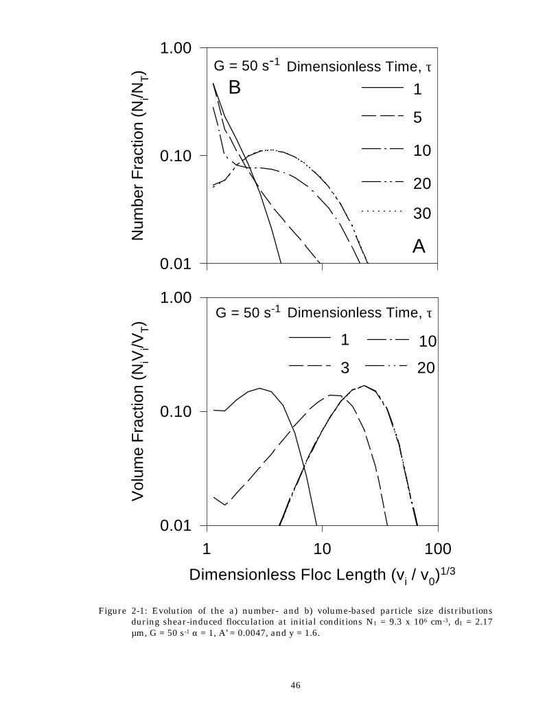
46

Figure 2-1: Evolution of the a) number- and b) volume-based particle size distributions during shear-induced flocculation at initial conditions N1 = 9.3 x 106 cm-3, d1 = 2.17 µm, G = 50 s-1 α = 1, A’ = 0.0047, and y = 1.6.

Num

ber

Fra

ctio

n (N

i/NT)

0.01

0.10

1.00Dimensionless Time, τG = 50 s-1

A

1

5

10

20

30

B

Dimensionless Floc Length (vi / v0)1/3

1 10 100

Vol

ume

Fra

ctio

n (N

iVi/V

T)

0.01

0.10

1.00Dimensionless Time, τG = 50 s-1

1

3

10

20

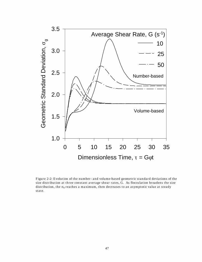
47

Figure 2-2: Evolution of the number- and volume-based geometric standard deviations of the size distribution at three constant average shear rates, G. As flocculation broadens the size distribution, the σg reaches a maximum, then decreases to an asymptotic value at steady state.

Dimensionless Time, τ = Gφt

0 5 10 15 20 25 30 35

Geo

met

ric S

tand

ard

Dev

iatio

n, σ

g

1.0

1.5

2.0

2.5

3.0

3.5

Volume-based

Number-based

Average Shear Rate, G (s-1)

10

25

50

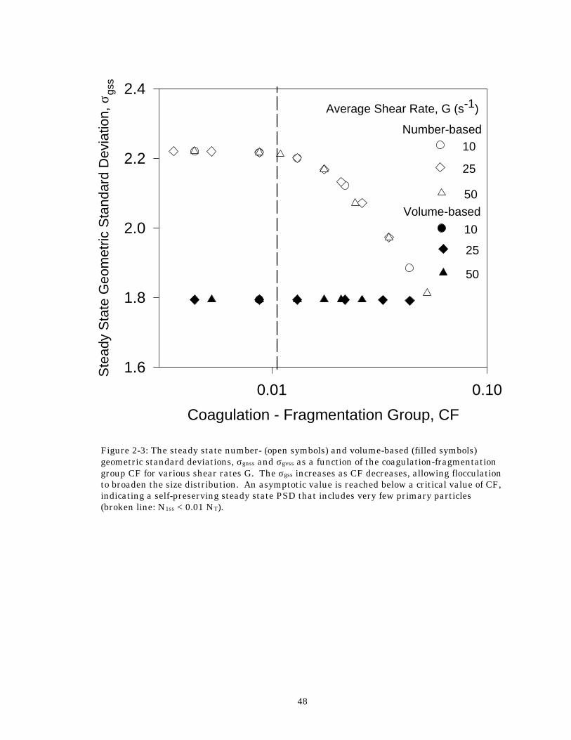
48

Figure 2-3: The steady state number- (open symbols) and volume-based (filled symbols) geometric standard deviations, σgnss and σgvss as a function of the coagulation-fragmentation group CF for various shear rates G. The σgss increases as CF decreases, allowing flocculation to broaden the size distribution. An asymptotic value is reached below a critical value of CF, indicating a self-preserving steady state PSD that includes very few primary particles (broken line: N1ss < 0.01 NT).

Coagulation - Fragmentation Group, CF

0.01 0.10

Ste

ady

Sta

te G

eom

etric

Sta

ndar

d D

evia

tion,

σgs

s

1.6

1.8

2.0

2.2

2.4

Volume-based

Number-based


10

25

50

10

25

50

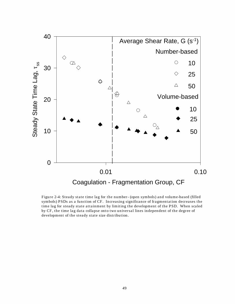
49

Figure 2-4: Steady state time lag for the number- (open symbols) and volume-based (filled symbols) PSDs as a function of CF. Increasing significance of fragmentation decreases the time lag for steady state attainment by limiting the development of the PSD. When scaled by CF, the time lag data collapse onto two universal lines independent of the degree of development of the steady state size distribution.

Coagulation - Fragmentation Group, CF

0.01 0.10

Ste

ady

Sta

te T

ime

Lag,

τss

0

10

20

30

40

Volume-based

Number-based


10

25

50

10

25

50

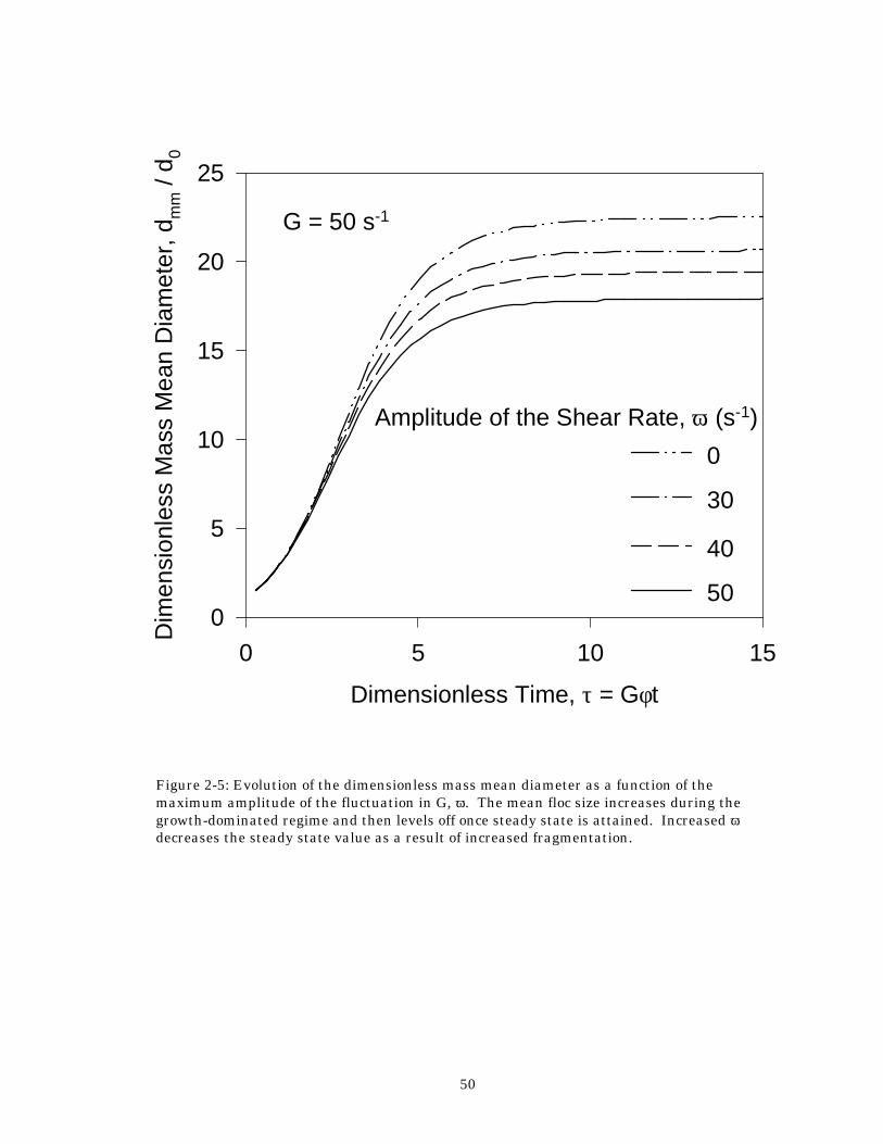
50

Figure 2-5: Evolution of the dimensionless mass mean diameter as a function of the maximum amplitude of the fluctuation in G, ω. The mean floc size increases during the growth-dominated regime and then levels off once steady state is attained. Increased ω decreases the steady state value as a result of increased fragmentation.


0 5 10 15

Dim

ensi

onle

ss M

ass

Mea

n D

iam

eter

, dm

m /

d 0

0

5

10

15

20

25

G = 50 s-1

Amplitude of the Shear Rate, ω (s-1)

50

40

30

0

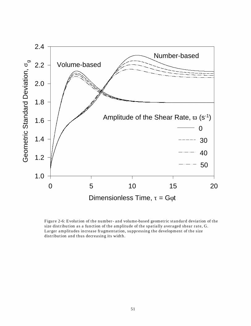
51

Figure 2-6: Evolution of the number- and volume-based geometric standard deviation of the size distribution as a function of the amplitude of the spatially averaged shear rate, G. Larger amplitudes increase fragmentation, suppressing the development of the size distribution and thus decreasing its width.


0 5 10 15 20

Geo

met

ric S

tand

ard

Dev

iatio

n, σ

g

1.0

1.2

1.4

1.6

1.8

2.0

2.2

2.4

Volume-basedNumber-based

Amplitude of the Shear Rate, ω (s-1)

0

30

40

50

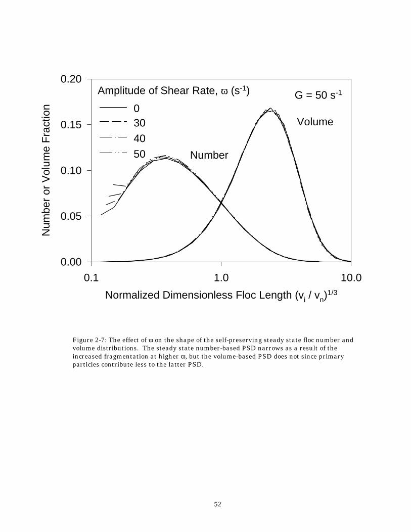
52

Figure 2-7: The effect of ω on the shape of the self-preserving steady state floc number and volume distributions. The steady state number-based PSD narrows as a result of the increased fragmentation at higher ω, but the volume-based PSD does not since primary particles contribute less to the latter PSD.

Normalized Dimensionless Floc Length (vi / vn)1/3

0.1 1.0 10.0

Num

ber

or V

olum

e F

ract

ion

0.00

0.05

0.10

0.15

0.20Amplitude of Shear Rate, ω (s-1) G = 50 s-1

Number

Volume0304050

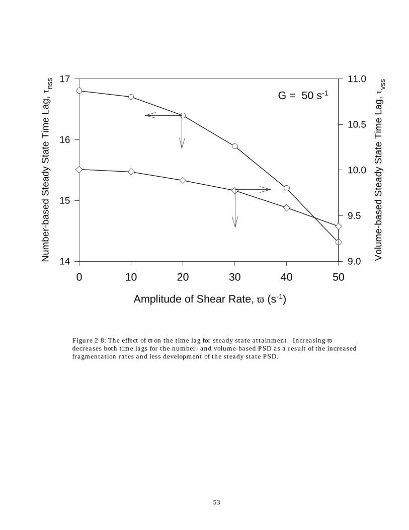
53

Figure 2-8: The effect of ω on the time lag for steady state attainment. Increasing ω decreases both time lags for the number- and volume-based PSD as a result of the increased fragmentation rates and less development of the steady state PSD.

Amplitude of Shear Rate, ω (s-1)

0 10 20 30 40 50

Num

ber-

base

d S

tead

y S

tate

Tim

e La

g, τ

nss

14

15

16

17

Vol

ume-

base

d S

tead

y S

tate

Tim

e La

g, τ

vss

9.0

9.5

10.0

10.5

11.0

G = 50 s-1

54

Chapter 3 - Effect of Impeller Type on Floc Size and Structure

The effect of impeller type and shear rate on the evolution of floc size and structure during shear-induced flocculation of polystyrene particles with aluminum sulfate is investigated by image analysis. One radial flow (six-blade Rushton turbine) and two axial flow (three-blade fluid foil, four-blade 45° pitch) impeller configurations are examined. The steady state average floc size is shown to depend on the frequency of recirculation to the impeller zone and its characteristic velocity gradient. The concepts of fractal geometry are used to characterize the floc structure. For all impellers, the two-dimensional floc fractal dimension, Dpf, increases during floc growth, indicating formation of more open structures. Later on, Dpf levels off at a steady state value as breakage becomes significant and the floc size distribution approaches steady state. The shear rate does not affect the steady state Dpf of the flocs within experimental uncertainty. This chapter has been published: Spicer, P. T., Keller, W. and Pratsinis, S. E., "The Effect of Impeller Type on Floc Size and Structure During Shear-Induced Flocculation," J. Colloid Interface Sci., 184, 112-122 (1996).

55

Introduction Solids removal efficiency by sedimentation or filtration depends on the structure of the flocs, as this determines the relationship between floc size and density. In addition, changes in floc structure within a suspension affect macroscopic properties like viscosity (Gillespie, 1983) altering the processing requirements of cell suspensions (Roels et al., 1988; Cooke, 1993; Shamlou and Tichener-Hooker, 1993). The porosity of flocs also determines the quality of compact parts made of ceramic particles (Pierre et al., 1995). Despite its significance in numerous disciplines, the dynamic evolution of sheared floc structures has not been studied experimentally. Most previous studies have evaluated the structure of flocs at steady state (Tambo and Watanabe, 1979; Klimpel and Hogg, 1986; Logan and Kilps, 1995). The evolution of the floc structure is equally important, however, as it determines the steady state characteristics of the flocs and their removal efficiency. Settling velocity measurements indicate an inverse relationship between floc size and density. The reduced floc density with increasing size is usually attributed to the incorporation of fluid into the floc structure. These porous flocs collide with each other to form increasingly porous structures (Francois and van Haute, 1984) until shear-induced fragmentation halts further growth of the floc size distribution. Floc structures can also be made more compact by shear-induced breakage or restructuring (Thomas, 1964; Sonntag and Russel, 1986; Francois, 1987; Jullien and Meakin, 1989; Clark and Flora, 1991) as illustrated in Figure 3-1. The growth, breakage and restructuring processes govern the development of floc structures and all three occur within the complex shear field of a stirred tank. Despite the relevance of the hydrodynamic flow field on flocculator performance, few fundamental studies of the effect of different flow fields on flocculation variables like floc size and structure have been carried out. Oldshue and Mady (1978) studied the effect of impeller type and flocculator volume on particle removal at a water treatment plant using turbidity measurements. They observed different particle removal efficiencies at constant shear rate, G, for the impellers examined. Glasgow (1990) compared the hydrodynamic behavior and flocculation performance of two perforated plastic paddle impeller assemblies: a 4-blade paddle and a paddle covered with cloth. The two impellers produced significantly different energy dissipation rates at the same impeller speeds, especially at low values. No significant difference between the two impellers was observed from average floc size and density measurements. McConnachie (1991) evaluated three impellers (paddle, picket gate, and branched paddle) by measurements of fluid turbulent intensity, local fluid velocity, and turbidity during flocculation. He observed that each impeller produced a minimum turbidity level at a similar power input, indicating no significant difference between the performance of the three impellers. Oldshue and Trussell (1991) found that the average shear rate in a stirred tank was a linear function of impeller speed, N, for the Rushton, 4-blade, and fluid foil impellers regardless of their size. However, the maximum shear rate varied linearly with impeller speed for the fluid foil impeller while it varied linearly with impeller tip speed, ND, for the other impellers in agreement with de Boer et al. (1989). The objective of this study is to describe the effect of impeller type (and thus hydrodynamic flow field) on the evolution of the average floc size and structure during flocculation of polystyrene particles with aluminum sulfate in a stirred tank. The floc size and structure are monitored as a function of time using image analysis, thus characterizing the structural events leading up to the attainment of steady state.

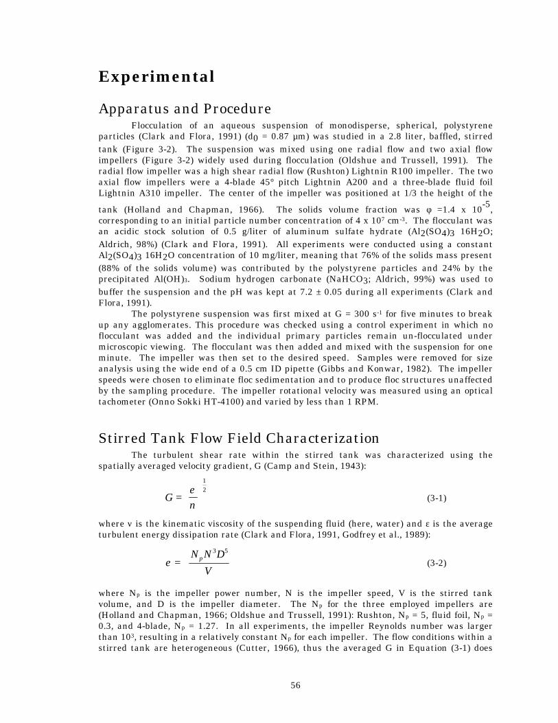
56

Experimental

Apparatus and Procedure Flocculation of an aqueous suspension of monodisperse, spherical, polystyrene particles (Clark and Flora, 1991) (d0 = 0.87 µm) was studied in a 2.8 liter, baffled, stirred tank (Figure 3-2). The suspension was mixed using one radial flow and two axial flow impellers (Figure 3-2) widely used during flocculation (Oldshue and Trussell, 1991). The radial flow impeller was a high shear radial flow (Rushton) Lightnin R100 impeller. The two axial flow impellers were a 4-blade 45° pitch Lightnin A200 and a three-blade fluid foil Lightnin A310 impeller. The center of the impeller was positioned at 1/3 the height of the

tank (Holland and Chapman, 1966). The solids volume fraction was φ =1.4 x 10-5, corresponding to an initial particle number concentration of 4 x 107 cm-3. The flocculant was an acidic stock solution of 0.5 g/liter of aluminum sulfate hydrate (Al2(SO4)3 16H2O; Aldrich, 98%) (Clark and Flora, 1991). All experiments were conducted using a constant Al2(SO4)3 16H2O concentration of 10 mg/liter, meaning that 76% of the solids mass present (88% of the solids volume) was contributed by the polystyrene particles and 24% by the precipitated Al(OH)3. Sodium hydrogen carbonate (NaHCO3; Aldrich, 99%) was used to buffer the suspension and the pH was kept at 7.2 ± 0.05 during all experiments (Clark and Flora, 1991). The polystyrene suspension was first mixed at G = 300 s-1 for five minutes to break up any agglomerates. This procedure was checked using a control experiment in which no flocculant was added and the individual primary particles remain un-flocculated under microscopic viewing. The flocculant was then added and mixed with the suspension for one minute. The impeller was then set to the desired speed. Samples were removed for size analysis using the wide end of a 0.5 cm ID pipette (Gibbs and Konwar, 1982). The impeller speeds were chosen to eliminate floc sedimentation and to produce floc structures unaffected by the sampling procedure. The impeller rotational velocity was measured using an optical tachometer (Onno Sokki HT-4100) and varied by less than 1 RPM.

Stirred Tank Flow Field Characterization The turbulent shear rate within the stirred tank was characterized using the spatially averaged velocity gradient, G (Camp and Stein, 1943):

G =

εν

12 (3-1)

where ν is the kinematic viscosity of the suspending fluid (here, water) and ε is the average turbulent energy dissipation rate (Clark and Flora, 1991, Godfrey et al., 1989):

ε =

N N D

Vp

3 5

(3-2)

where Np is the impeller power number, N is the impeller speed, V is the stirred tank volume, and D is the impeller diameter. The Np for the three employed impellers are (Holland and Chapman, 1966; Oldshue and Trussell, 1991): Rushton, Np = 5, fluid foil, Np = 0.3, and 4-blade, Np = 1.27. In all experiments, the impeller Reynolds number was larger than 103, resulting in a relatively constant Np for each impeller. The flow conditions within a stirred tank are heterogeneous (Cutter, 1966), thus the averaged G in Equation (3-1) does

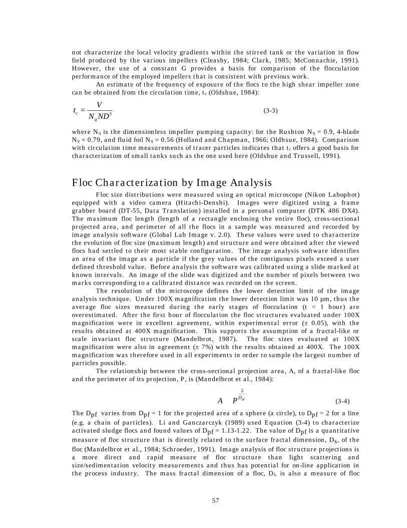
57

not characterize the local velocity gradients within the stirred tank or the variation in flow field produced by the various impellers (Cleasby, 1984; Clark, 1985; McConnachie, 1991). However, the use of a constant G provides a basis for comparison of the flocculation performance of the employed impellers that is consistent with previous work. An estimate of the frequency of exposure of the flocs to the high shear impeller zone can be obtained from the circulation time, tc (Oldshue, 1984):

tV

N NDcq

= 3 (3-3)

where Nq is the dimensionless impeller pumping capacity: for the Rushton Nq = 0.9, 4-blade Nq = 0.79, and fluid foil Nq = 0.56 (Holland and Chapman, 1966; Oldhsue, 1984). Comparison with circulation time measurements of tracer particles indicates that tc offers a good basis for characterization of small tanks such as the one used here (Oldshue and Trussell, 1991).

Floc Characterization by Image Analysis Floc size distributions were measured using an optical microscope (Nikon Labophot) equipped with a video camera (Hitachi-Denshi). Images were digitized using a frame grabber board (DT-55, Data Translation) installed in a personal computer (DTK 486 DX4). The maximum floc length (length of a rectangle enclosing the entire floc), cross-sectional projected area, and perimeter of all the flocs in a sample was measured and recorded by image analysis software (Global Lab Image v. 2.0). These values were used to characterize the evolution of floc size (maximum length) and structure and were obtained after the viewed flocs had settled to their most stable configuration. The image analysis software identifies an area of the image as a particle if the grey values of the contiguous pixels exceed a user defined threshold value. Before analysis the software was calibrated using a slide marked at known intervals. An image of the slide was digitized and the number of pixels between two marks corresponding to a calibrated distance was recorded on the screen. The resolution of the microscope defines the lower detection limit of the image analysis technique. Under 100X magnification the lower detection limit was 10 µm, thus the average floc sizes measured during the early stages of flocculation (t < 1 hour) are overestimated. After the first hour of flocculation the floc structures evaluated under 100X magnification were in excellent agreement, within experimental error (± 0.05), with the results obtained at 400X magnification. This supports the assumption of a fractal-like or scale invariant floc structure (Mandelbrot, 1987). The floc sizes evaluated at 100X magnification were also in agreement (± 7%) with the results obtained at 400X. The 100X magnification was therefore used in all experiments in order to sample the largest number of particles possible. The relationship between the cross-sectional projection area, A, of a fractal-like floc and the perimeter of its projection, P, is (Mandelbrot et al., 1984):

A P Dpf∝2

(3-4)

The Dpf varies from Dpf = 1 for the projected area of a sphere (a circle), to Dpf = 2 for a line (e.g. a chain of particles). Li and Ganczarczyk (1989) used Equation (3-4) to characterize activated sludge flocs and found values of Dpf = 1.13-1.22. The value of Dpf is a quantitative measure of floc structure that is directly related to the surface fractal dimension, Ds, of the floc (Mandelbrot et al., 1984; Schroeder, 1991). Image analysis of floc structure projections is a more direct and rapid measure of floc structure than light scattering and size/sedimentation velocity measurements and thus has potential for on-line application in the process industry. The mass fractal dimension of a floc, Df, is also a measure of floc

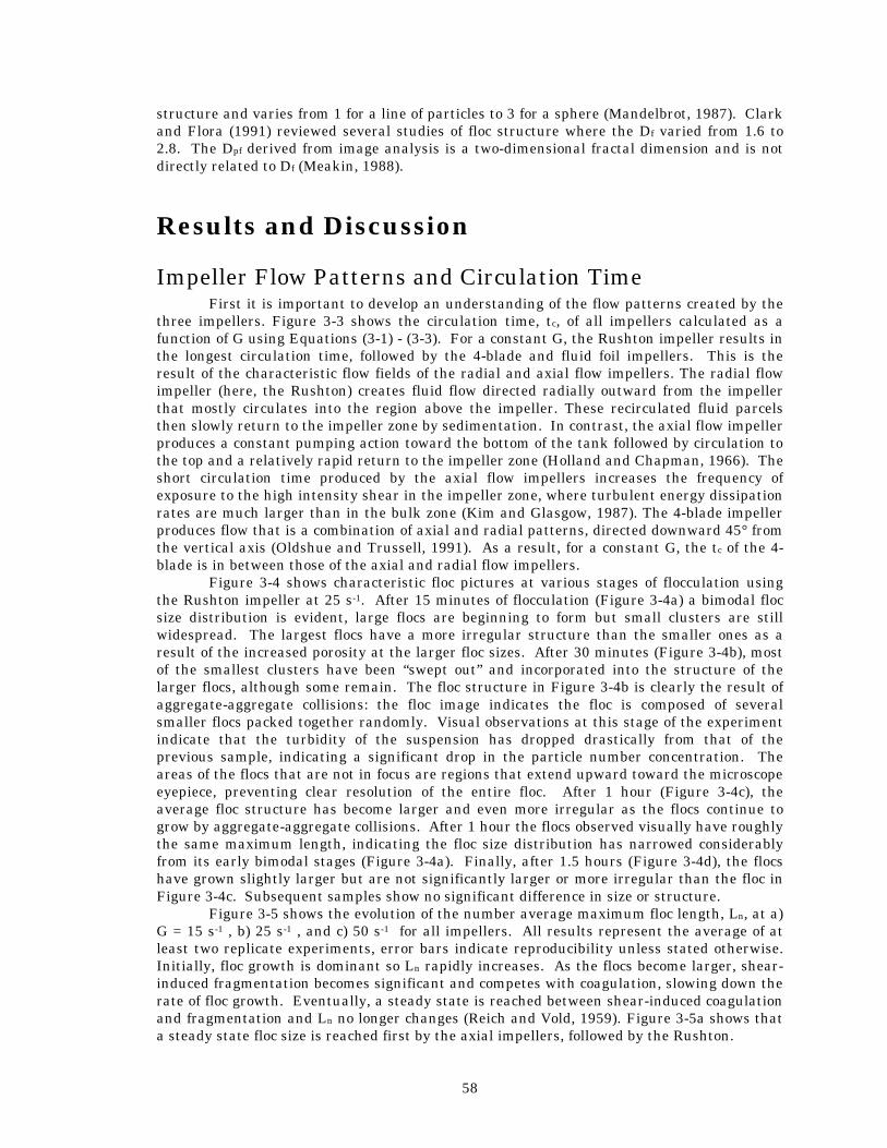
58

structure and varies from 1 for a line of particles to 3 for a sphere (Mandelbrot, 1987). Clark and Flora (1991) reviewed several studies of floc structure where the Df varied from 1.6 to 2.8. The Dpf derived from image analysis is a two-dimensional fractal dimension and is not directly related to Df (Meakin, 1988).

Results and Discussion

Impeller Flow Patterns and Circulation Time First it is important to develop an understanding of the flow patterns created by the three impellers. Figure 3-3 shows the circulation time, tc, of all impellers calculated as a function of G using Equations (3-1) - (3-3). For a constant G, the Rushton impeller results in the longest circulation time, followed by the 4-blade and fluid foil impellers. This is the result of the characteristic flow fields of the radial and axial flow impellers. The radial flow impeller (here, the Rushton) creates fluid flow directed radially outward from the impeller that mostly circulates into the region above the impeller. These recirculated fluid parcels then slowly return to the impeller zone by sedimentation. In contrast, the axial flow impeller produces a constant pumping action toward the bottom of the tank followed by circulation to the top and a relatively rapid return to the impeller zone (Holland and Chapman, 1966). The short circulation time produced by the axial flow impellers increases the frequency of exposure to the high intensity shear in the impeller zone, where turbulent energy dissipation rates are much larger than in the bulk zone (Kim and Glasgow, 1987). The 4-blade impeller produces flow that is a combination of axial and radial patterns, directed downward 45° from the vertical axis (Oldshue and Trussell, 1991). As a result, for a constant G, the tc of the 4-blade is in between those of the axial and radial flow impellers. Figure 3-4 shows characteristic floc pictures at various stages of flocculation using the Rushton impeller at 25 s-1. After 15 minutes of flocculation (Figure 3-4a) a bimodal floc size distribution is evident, large flocs are beginning to form but small clusters are still widespread. The largest flocs have a more irregular structure than the smaller ones as a result of the increased porosity at the larger floc sizes. After 30 minutes (Figure 3-4b), most of the smallest clusters have been “swept out” and incorporated into the structure of the larger flocs, although some remain. The floc structure in Figure 3-4b is clearly the result of aggregate-aggregate collisions: the floc image indicates the floc is composed of several smaller flocs packed together randomly. Visual observations at this stage of the experiment indicate that the turbidity of the suspension has dropped drastically from that of the previous sample, indicating a significant drop in the particle number concentration. The areas of the flocs that are not in focus are regions that extend upward toward the microscope eyepiece, preventing clear resolution of the entire floc. After 1 hour (Figure 3-4c), the average floc structure has become larger and even more irregular as the flocs continue to grow by aggregate-aggregate collisions. After 1 hour the flocs observed visually have roughly the same maximum length, indicating the floc size distribution has narrowed considerably from its early bimodal stages (Figure 3-4a). Finally, after 1.5 hours (Figure 3-4d), the flocs have grown slightly larger but are not significantly larger or more irregular than the floc in Figure 3-4c. Subsequent samples show no significant difference in size or structure. Figure 3-5 shows the evolution of the number average maximum floc length, Ln, at a) G = 15 s-1 , b) 25 s-1 , and c) 50 s-1 for all impellers. All results represent the average of at least two replicate experiments, error bars indicate reproducibility unless stated otherwise. Initially, floc growth is dominant so Ln rapidly increases. As the flocs become larger, shear-induced fragmentation becomes significant and competes with coagulation, slowing down the rate of floc growth. Eventually, a steady state is reached between shear-induced coagulation and fragmentation and Ln no longer changes (Reich and Vold, 1959). Figure 3-5a shows that a steady state floc size is reached first by the axial impellers, followed by the Rushton.

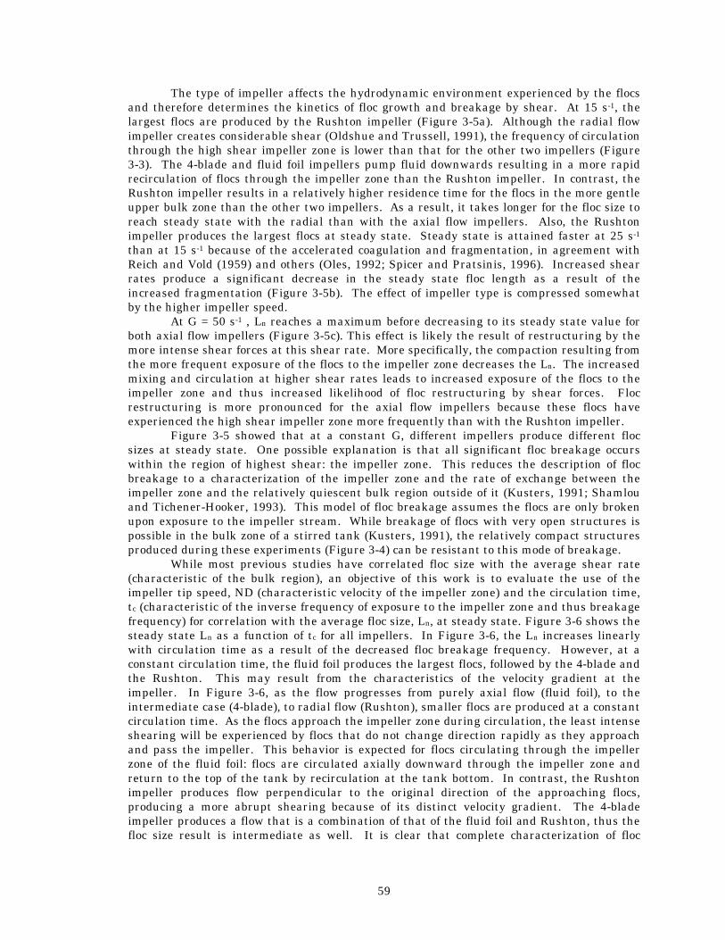
59

The type of impeller affects the hydrodynamic environment experienced by the flocs and therefore determines the kinetics of floc growth and breakage by shear. At 15 s-1, the largest flocs are produced by the Rushton impeller (Figure 3-5a). Although the radial flow impeller creates considerable shear (Oldshue and Trussell, 1991), the frequency of circulation through the high shear impeller zone is lower than that for the other two impellers (Figure 3-3). The 4-blade and fluid foil impellers pump fluid downwards resulting in a more rapid recirculation of flocs through the impeller zone than the Rushton impeller. In contrast, the Rushton impeller results in a relatively higher residence time for the flocs in the more gentle upper bulk zone than the other two impellers. As a result, it takes longer for the floc size to reach steady state with the radial than with the axial flow impellers. Also, the Rushton impeller produces the largest flocs at steady state. Steady state is attained faster at 25 s-1 than at 15 s-1 because of the accelerated coagulation and fragmentation, in agreement with Reich and Vold (1959) and others (Oles, 1992; Spicer and Pratsinis, 1996). Increased shear rates produce a significant decrease in the steady state floc length as a result of the increased fragmentation (Figure 3-5b). The effect of impeller type is compressed somewhat by the higher impeller speed. At G = 50 s-1 , Ln reaches a maximum before decreasing to its steady state value for both axial flow impellers (Figure 3-5c). This effect is likely the result of restructuring by the more intense shear forces at this shear rate. More specifically, the compaction resulting from the more frequent exposure of the flocs to the impeller zone decreases the Ln. The increased mixing and circulation at higher shear rates leads to increased exposure of the flocs to the impeller zone and thus increased likelihood of floc restructuring by shear forces. Floc restructuring is more pronounced for the axial flow impellers because these flocs have experienced the high shear impeller zone more frequently than with the Rushton impeller. Figure 3-5 showed that at a constant G, different impellers produce different floc sizes at steady state. One possible explanation is that all significant floc breakage occurs within the region of highest shear: the impeller zone. This reduces the description of floc breakage to a characterization of the impeller zone and the rate of exchange between the impeller zone and the relatively quiescent bulk region outside of it (Kusters, 1991; Shamlou and Tichener-Hooker, 1993). This model of floc breakage assumes the flocs are only broken upon exposure to the impeller stream. While breakage of flocs with very open structures is possible in the bulk zone of a stirred tank (Kusters, 1991), the relatively compact structures produced during these experiments (Figure 3-4) can be resistant to this mode of breakage. While most previous studies have correlated floc size with the average shear rate (characteristic of the bulk region), an objective of this work is to evaluate the use of the impeller tip speed, ND (characteristic velocity of the impeller zone) and the circulation time, tc (characteristic of the inverse frequency of exposure to the impeller zone and thus breakage frequency) for correlation with the average floc size, Ln, at steady state. Figure 3-6 shows the steady state Ln as a function of tc for all impellers. In Figure 3-6, the Ln increases linearly with circulation time as a result of the decreased floc breakage frequency. However, at a constant circulation time, the fluid foil produces the largest flocs, followed by the 4-blade and the Rushton. This may result from the characteristics of the velocity gradient at the impeller. In Figure 3-6, as the flow progresses from purely axial flow (fluid foil), to the intermediate case (4-blade), to radial flow (Rushton), smaller flocs are produced at a constant circulation time. As the flocs approach the impeller zone during circulation, the least intense shearing will be experienced by flocs that do not change direction rapidly as they approach and pass the impeller. This behavior is expected for flocs circulating through the impeller zone of the fluid foil: flocs are circulated axially downward through the impeller zone and return to the top of the tank by recirculation at the tank bottom. In contrast, the Rushton impeller produces flow perpendicular to the original direction of the approaching flocs, producing a more abrupt shearing because of its distinct velocity gradient. The 4-blade impeller produces a flow that is a combination of that of the fluid foil and Rushton, thus the floc size result is intermediate as well. It is clear that complete characterization of floc

60

breakage frequency in the impeller zone requires knowledge not only of the frequency of floc exposure to the impeller zone but also of the characteristic velocity gradient in the impeller zone. The speed of the impeller tip, ND, is indicative of the impeller zone velocity gradient (Oldshue and Trussell, 1991). Figure 3-7 shows the effect of impeller tip speed on the steady state floc size for all three impellers. For all impellers, increasing the impeller tip speed decreases the steady state average maximum floc length. The data are best correlated by a power law function, similar to the relationships found between floc size and the average shear rate, G (Tambo and Watanabe, 1979). It should be noted, however, that a power law fit of the steady state Ln as a function of G yielded a weaker correlation (R2 = 0.796) than for tc (R2 = 0.882) or ND (R2 = 0.855). At a constant tip speed, the same trend observed in Figure 3-6 is seen in Figure 3-7: the largest flocs are produced by the fluid foil, followed by the 4-blade and the Rushton. This may also result from the different direction of the velocity gradient at the impeller with changing impeller types. The results in Figure 3-6 and Figure 3-7 indicate that the frequency of exposure to the impeller zone and the zone’s characteristic velocity gradient are important design parameters for minimizing floc breakage and thus maximizing floc size.

Effect of Impeller Type and Shear Rate on the Evolution of Floc Structure Figure 3-8 shows the evolution of the perimeter-based fractal dimension for a) G = 15 s-1 , b) 25 s-1 , and c) 50 s-1 for the three impellers. Initially the Dpf increases, indicating that more open floc structures are formed as floc growth dominates, regardless of the impeller type. Later on, Dpf reaches steady state as fragmentation becomes significant and impedes the production of more irregular structures. The impeller type does not appear to influence the evolution of the Dpf, since the data in Figure 3-8a closely follow the same evolution pattern. More scatter in Dpf is observed at G = 25 s-1 (Figure 3-8b) than at G = 15 s-1 (Figure 3-8a), although this decreases as steady state is approached and the distribution of floc structures narrows (Spicer and Pratsinis, 1996). For all impellers, the evolution of Dpf collapses onto one curve at a constant shear rate. A slightly higher steady state value of Dpf is reached at 25 s-1 than at 15 s-1, although this may not be significant within the uncertainty of the Dpf determination. At G = 50 s-1, the Dpf of the flocs increases rapidly at early times, indicating the formation of open flocs while shear-induced growth dominates (Figure 3-8c). From then on, significant floc breakage takes place, making the floc structure more compact (decreasing Dpf) as a steady state is attained with respect to floc size and structure. This is more significant for the two axial flow impellers: in Figure 3-8c the Dpf produced by these impellers gradually decreases to its steady state value. This is consistent with the maximum in Ln observed in Figure 3-5c at t = 1 hour for the axial flow impellers. Thus, it is possible that the more open floc structures (larger Dpf) increase the floc collision rates and subsequently their growth resulting in larger particles (larger Ln). Later on, however, these rather weak flocs break by shear-induced fragmentation and reach a steady state as with the lower shear rates.

Conclusions The evolution of the polystyrene-alum floc structures produced by various impellers and spatially averaged velocity gradients, G, has been investigated. The average floc length, Ln, increased rapidly during floc growth and leveled off at a steady state value that increased with decreasing G with all impellers. The Rushton impeller produced the largest flocs,

61

followed by the 4-blade and the fluid foil impellers at all G values. The Rushton impeller results in the largest circulation time and thus the lowest frequency of exposure to the impeller zone in the stirred tank. However, at a constant circulation time and impeller tip speed, the fluid foil impeller produced the largest flocs, followed by the 4-blade and the Rushton impellers. This is attributed to the greater shearing action of the radial than the axial impeller in the impeller zone.

The two-dimensional fractal dimension of the flocs, Dpf, was used to quantify their structure. The Dpf of flocs produced by all three impellers increased rapidly during the early (growth-dominated) stage of flocculation. The evolution of Dpf was not influenced by impeller type at G = 15 and 25 s-1. At G = 50 s-1, a maximum in Dpf is observed prior to attainment of steady state for the two axial flow impellers as a result of the increased floc exposure at the impeller zone. The G does not affect the steady state Dpf value of the flocs at constant flocculant concentration within experimental uncertainty.

62

Notation A aggregate cross-sectional area (µm2) d0 primary particle diameter (µm) D impeller diameter (cm) Dpf perimeter-based aggregate fractal dimension (-) Df fractal dimension (-) G spatially averaged shear rate (s-1) N impeller rotational rate (s-1) Ln aggregate collision diameter (µm) ND impeller tip speed (cm/s) Np impeller power number (-) Nq impeller flow number (-) N0 initial number concentration (# / cm3) P aggregate perimeter (µm) t time (s) tc circulation time (s) V tank volume (liter)

Greek Letters ε energy dissipation rate (cm2/s3) φ solids volume fraction (-) η Kolmogorov microscale (µm) ν kinematic viscosity (cm2 / s)

63

References Blatz, P. J. and Tobolsky, A. V., “Note on the Kinetics of Systems Manifesting Simultaneous

Polymerization-Depolymerization Phenomena,” J. Phys. Chem., 49, 77-80 (1945). Camp, T. R. and Stein, P. G., "Velocity Gradients and Internal Work in Fluid Motion," J.

Boston Soc. Civ. Eng., 30, 219, (1943). Clark, M. M., “Critique of Camp and Stein’s RMS Velocity Gradient,” J. Env. Eng., 111, 741-

754 (1985). Clark, M. M., and Flora, J. R. V., "Floc Restructuring in Varied Turbulent Mixing," J. Colloid

and Interface Sci., 147, 407-421 (1991). Cleasby, J. L., “Is Velocity Gradient a Valid Turbulent Flocculation Parameter?,” J. Env.

Eng., 110, 875-897 (1984). Cooke, M., “Application of Model Suspensions in the Design of Fermenters,” in Processing of

Solid-Liquid Suspensions, P. A. Shamlou, ed., Butterworth Heinemann, Oxford, 192 (1993).

Cutter, L. A., “Flow and Turbulence in a Stirred Tank,” AIChE J., 12, 35-45 (1966). de Boer, G. B. J., Hoedemakers, G. F. M., and Thoenes, D., “Coagulation in Turbulent Flow:

Part I,” Chem. Eng. Res. Des., 67, 301-307 (1989). Francois, R. J. and Van Haute, A. A., "Floc Strength Measurements Giving Experimental

Support for a Four Level Floc Structure," in Chemistry for the Protection of the Environment, Elsevier, Amsterdam, 221-234 (1984).

Francois, R. J., "Ageing of Aluminum Hydroxide Flocs," Water Res., 21, 523-531 (1987). Gibbs, R. J. and Konwar, L. N., "Effect of Pipetting on Mineral Flocs," Env. Sci. Tech., 16,

119-121 (1982). Gillespie, T., “The Effect of Aggregation and Particle Size Distribution on the Viscosity of

Newtonian Suspensions,” J. Colloid Interface Sci., 94, 166-173 (1983). Glasgow, L. A., "Aggregate Characteristics and Turbulence in Flocculation Basins," Chem.

Eng. Commun., 98, 155-171 (1990). Godfrey, J. C., Obi, F. I. N., and Reeve, R. N., “Measuring Drop Size in Continuous Liquid-

Liquid Mixers,” Chem. Eng. Prog., 85, 61-69 (1989). Holland, F. A. and Chapman, F. S., Liquid Mixing and Processing in Stirred Tanks,

Reinhold, London, (1966). Jullien, R. and Meakin, P., “Simple Models for the Restructuring of Three-Dimensional

Ballistic Aggregates,” J. Colloid Interface Sci., 127, 265-272 (1989). Kim, Y. H. and Glasgow, L. A., "Simulation of Aggregate Growth and Breakage in Stirred

Tanks," Industrial & Engineering Chemistry Research, 26 1604-1609 (1987). Klimpel, R. C. and Hogg, R., "Effects of Flocculation Conditions on Agglomerate Structure,"

J. Colloid Interface Sci., 113, 121-131 (1986). Kusters, K. A., "The Influence of Turbulence on Aggregation of Small Particles in Agitated

Vessels," Ph. D. Dissertation, Eindhoven University of Technology, The Netherlands, (1991).

Li, D., and Ganczarczyk, J. J., "Fractal Geometry of Particle Aggregates Generated in Water and Wastewater Treatment Processes," Env. Sci. Tech., 23, 1385-1389 (1989).

Logan, B. E. and Kilps, J. R., “Fractal Dimensions of Aggregates formed in Different Fluid Mechanical Environments,” Water Res., 29, 443-453 (1995).


Mandelbrot, B. B., Passoja, D. E., and Paullay, A. J., “Fractal Character of Fracture Surfaces of Metals,” Nature, 308, 721-722 (1984).

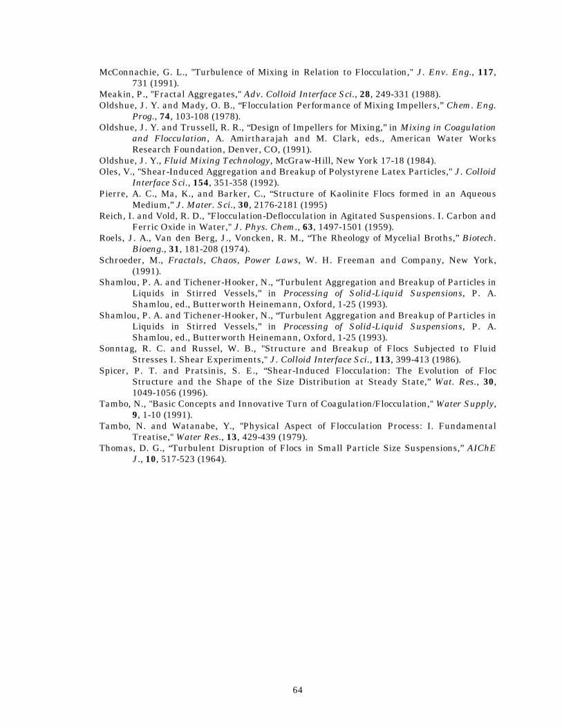
64

McConnachie, G. L., "Turbulence of Mixing in Relation to Flocculation," J. Env. Eng., 117, 731 (1991).

Meakin, P., "Fractal Aggregates," Adv. Colloid Interface Sci., 28, 249-331 (1988). Oldshue, J. Y. and Mady, O. B., “Flocculation Performance of Mixing Impellers,” Chem. Eng.

Prog., 74, 103-108 (1978). Oldshue, J. Y. and Trussell, R. R., “Design of Impellers for Mixing,” in Mixing in Coagulation

and Flocculation, A. Amirtharajah and M. Clark, eds., American Water Works Research Foundation, Denver, CO, (1991).

Oldshue, J. Y., Fluid Mixing Technology, McGraw-Hill, New York 17-18 (1984). Oles, V., "Shear-Induced Aggregation and Breakup of Polystyrene Latex Particles," J. Colloid

Interface Sci., 154, 351-358 (1992). Pierre, A. C., Ma, K., and Barker, C., “Structure of Kaolinite Flocs formed in an Aqueous

Medium,” J. Mater. Sci., 30, 2176-2181 (1995) Reich, I. and Vold, R. D., "Flocculation-Deflocculation in Agitated Suspensions. I. Carbon and

Ferric Oxide in Water," J. Phys. Chem., 63, 1497-1501 (1959). Roels, J. A., Van den Berg, J., Voncken, R. M., “The Rheology of Mycelial Broths,” Biotech.

Bioeng., 31, 181-208 (1974). Schroeder, M., Fractals, Chaos, Power Laws, W. H. Freeman and Company, New York,

(1991). Shamlou, P. A. and Tichener-Hooker, N., “Turbulent Aggregation and Breakup of Particles in

Liquids in Stirred Vessels,” in Processing of Solid-Liquid Suspensions, P. A. Shamlou, ed., Butterworth Heinemann, Oxford, 1-25 (1993).







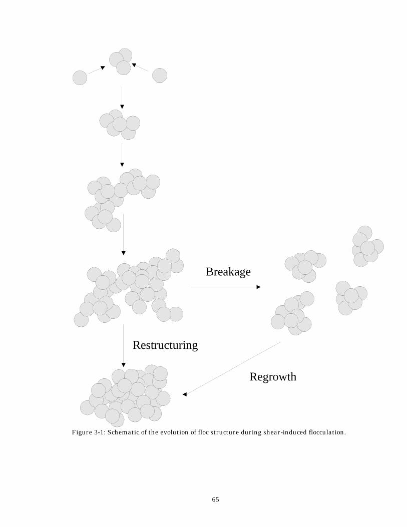
65

Figure 3-1: Schematic of the evolution of floc structure during shear-induced flocculation.

Regrowth

Restructuring

Breakage

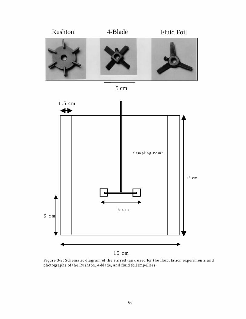
66

Figure 3-2: Schematic diagram of the stirred tank used for the flocculation experiments and photographs of the Rushton, 4-blade, and fluid foil impellers.

1 5 c m

1 5 c m

1 .5 cm

5 c m

S a m p lin g P o in t

5 c m

Rushton 4-Blade Fluid Foil

5 cm

67

Figure 3-3: Calculated circulation times, tc, as a function of G for all three impellers.

Spatially Averaged Shear Rate, G (s-1)

0 10 20 30 40 50

Circ

ulat

ion

Tim

e, t c

(s)

0

10

20

30

40

50

60

Rushton

4-blade

Fluid Foil

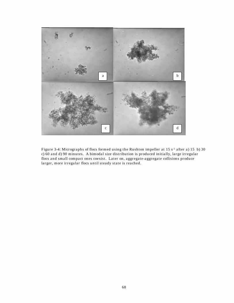
68

Figure 3-4: Micrographs of flocs formed using the Rushton impeller at 15 s-1 after a) 15 b) 30 c) 60 and d) 90 minutes. A bimodal size distribution is produced initially, large irregular flocs and small compact ones coexist. Later on, aggregate-aggregate collisions produce larger, more irregular flocs until steady state is reached.

a b

c d

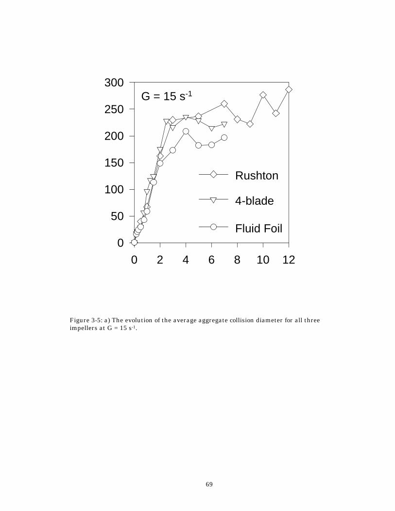
69

Figure 3-5: a) The evolution of the average aggregate collision diameter for all three impellers at G = 15 s-1.

0 2 4 6 8 10 120

50

100

150

200

250

300G = 15 s-1

Rushton

4-blade

Fluid Foil

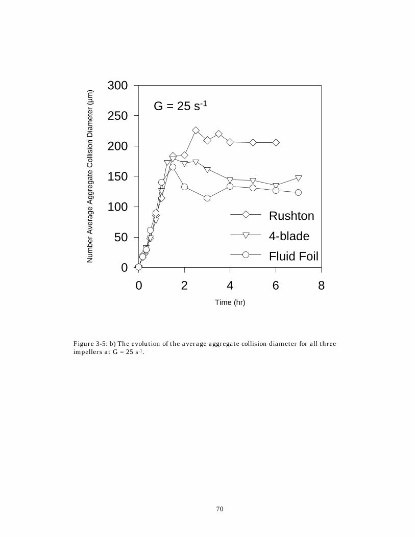
70

Figure 3-5: b) The evolution of the average aggregate collision diameter for all three impellers at G = 25 s-1.

Time (hr)

0 2 4 6 8

Num

ber

Ave

rage

Agg

rega

te C

ollis

ion

Dia

met

er (

µm)

0

50

100

150

200

250

300

G = 25 s-1

Rushton

4-blade

Fluid Foil

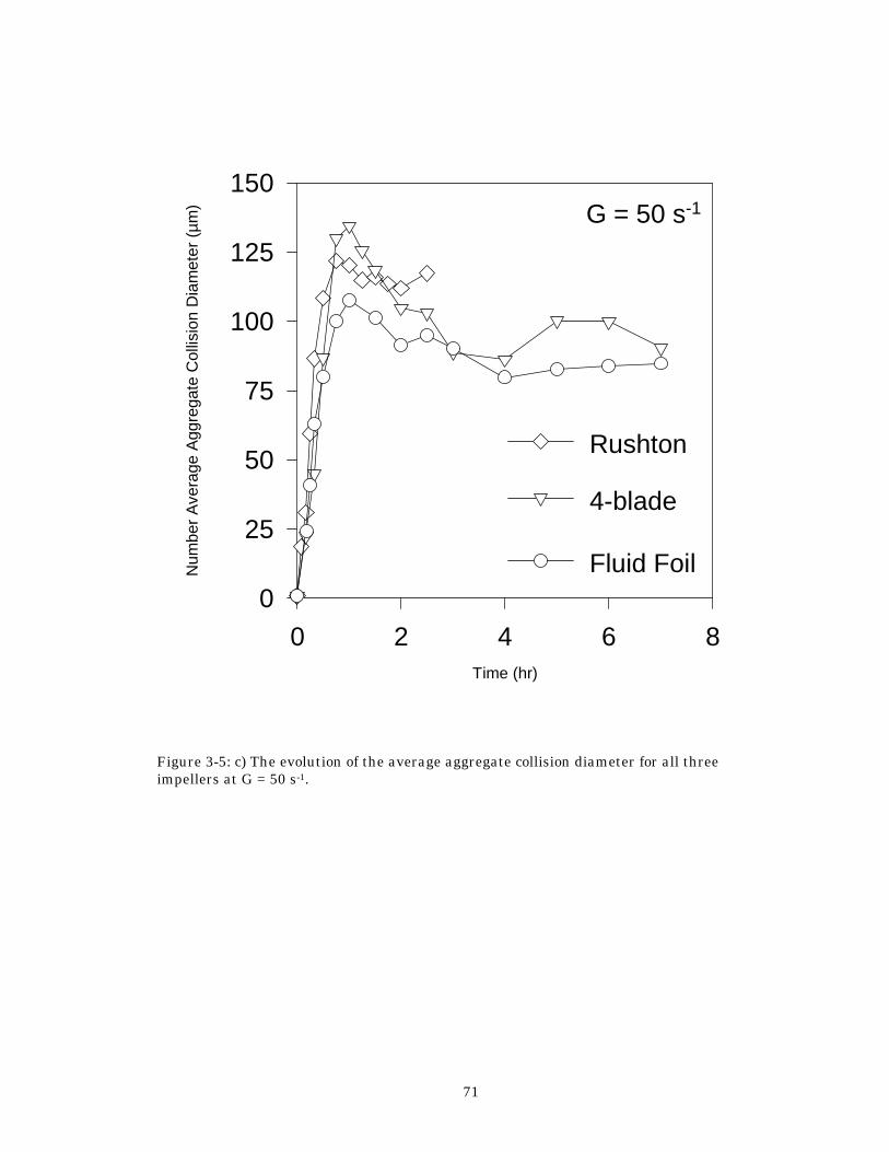
71

Figure 3-5: c) The evolution of the average aggregate collision diameter for all three impellers at G = 50 s-1.

Time (hr)

0 2 4 6 8

Num

ber

Ave

rage

Agg

rega

te C

ollis

ion

Dia

met

er (

µm)

0

25

50

75

100

125

150G = 50 s-1

Rushton

4-blade

Fluid Foil

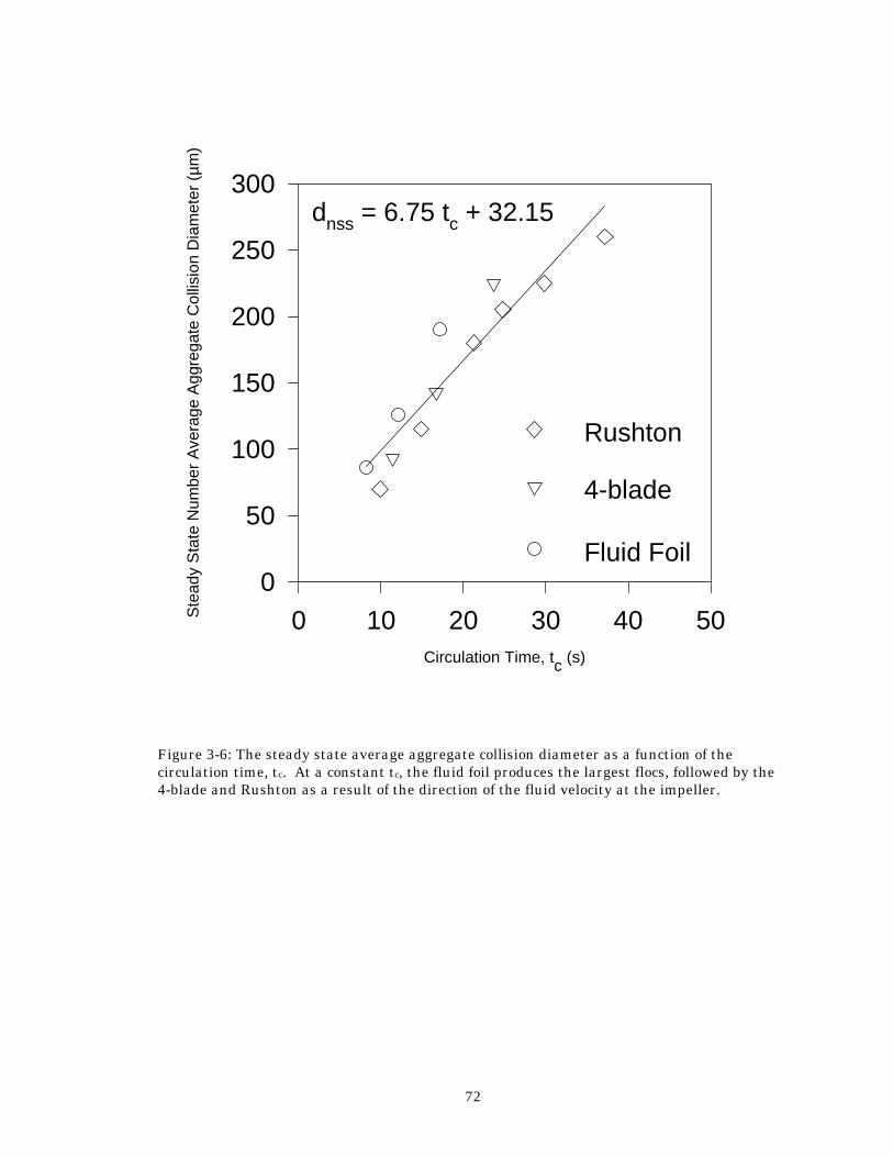
72

Figure 3-6: The steady state average aggregate collision diameter as a function of the circulation time, tc. At a constant tc, the fluid foil produces the largest flocs, followed by the 4-blade and Rushton as a result of the direction of the fluid velocity at the impeller.

Circulation Time, tc (s)

0 10 20 30 40 50Ste

ady

Sta

te N

umbe

r A

vera

ge A

ggre

gate

Col

lisio

n D

iam

eter

(µm

)

0

50

100

150

200

250

300

Rushton

4-blade

Fluid Foil

dnss = 6.75 tc + 32.15

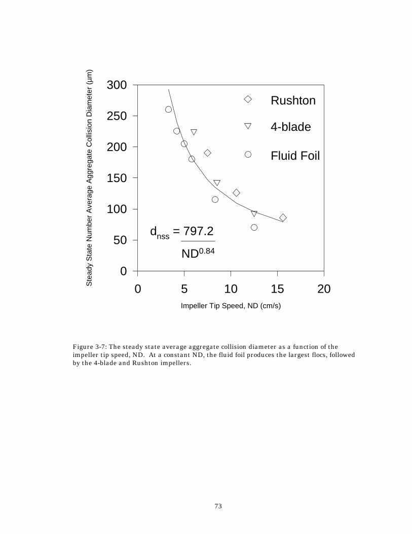
73

Figure 3-7: The steady state average aggregate collision diameter as a function of the impeller tip speed, ND. At a constant ND, the fluid foil produces the largest flocs, followed by the 4-blade and Rushton impellers.

Impeller Tip Speed, ND (cm/s)

0 5 10 15 20Ste

ady

Sta

te N

umbe

r A

vera

ge A

ggre

gate

Col

lisio

n D

iam

eter

(µm

)

0

50

100

150

200

250

300Rushton

4-blade

Fluid Foil

dnss = 797.2

ND0.84

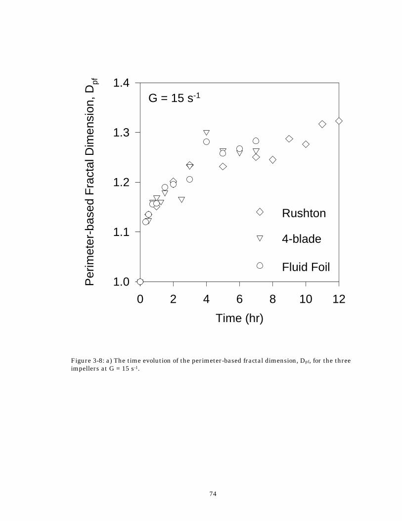
74

Figure 3-8: a) The time evolution of the perimeter-based fractal dimension, Dpf, for the three impellers at G = 15 s-1.

Time (hr)

0 2 4 6 8 10 12

Per

imet

er-b

ased

Fra

ctal

Dim

ensi

on, D

pf

1.0

1.1

1.2

1.3

1.4G = 15 s-1

Rushton

4-blade

Fluid Foil

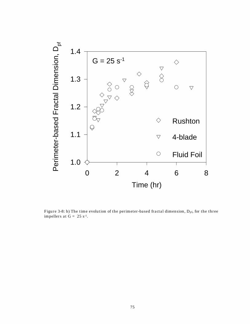
75

Figure 3-8: b) The time evolution of the perimeter-based fractal dimension, Dpf, for the three impellers at G = 25 s-1.

Time (hr)

0 2 4 6 8Per

imet

er-b

ased

Fra

ctal

Dim

ensi

on, D

pf

1.0

1.1

1.2

1.3

1.4G = 25 s-1

Rushton

4-blade

Fluid Foil

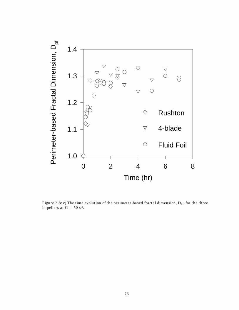
76

Figure 3-8: c) The time evolution of the perimeter-based fractal dimension, Dpf, for the three impellers at G = 50 s-1.

Time (hr)

0 2 4 6 8Per

imet

er-b

ased

Fra

ctal

Dim

ensi

on, D

pf

1.0

1.1

1.2

1.3

1.4

Rushton

4-blade

Fluid Foil

77

Chapter 4 - Effect of Shear Schedule on Particle Size and Structure The effect of shear history on the evolution of the polystyrene-alum floc size, density, and structure is investigated by small angle light scattering during cycled-shear and tapered-shear flocculation in a stirred tank using a Rushton impeller. The floc structure is characterized by the mass fractal dimension, Df, and the relative floc density. During turbulent shear flocculation, small floc structures are shown to be more open (Df = 2.1) than larger floc structures (Df = 2.5) as a result of shear-induced restructuring during steady state attainment. Flocs produced by cycled-shear flocculation are grown at shear rate G = 50 s-1 for 30 minutes, are fragmented at Gb = 100, 300, or 500 s-1 for one minute and then are regrown at G = 50 s-1. This shear schedule decreases the floc size but compacts the floc structure. When flocs are produced by gradual reduction of the shear rate from G = 300 s-1 to 50 s-1 (tapered-shear flocculation), smaller though equally dense flocs are produced compared to cycled-shear flocculation. The cycled-shear flocculation method produces the largest flocs with the highest potential for sedimentation when the fragmentation shear rate is Gb = 300 s-

1. This chapter has been published: Spicer, P. T., Pratsinis, S. E., Raper, J., Amal, R., Bushell, G. and Meesters, G., "Effect of Shear Schedule on Particle Size, Density, and Structure During Flocculation in Stirred Tanks," Powder Technol., 97, 26-34 (1998).

78

Introduction After a characteristic time of shear-induced flocculation, a steady state is reached between coagulation and fragmentation and the floc size distribution no longer changes (Reich and Vold, 1959). More recently, it has been shown that this steady state size distribution, scaled with the average floc size, does not depend on the applied shear rate (Spicer and Pratsinis, 1996a, b). A change in the applied shear rate drives a suspension at steady state to a new steady state. By lowering or raising the shear rate, larger or smaller flocs are formed, respectively. After the second steady state has been attained, if the original shear rate is then re-applied, two types of behavior have been observed experimentally: reversible and irreversible. For particle suspensions destabilized with an ionic salt (i.e. NaCl), when the original shear rate is re-applied, the steady state average floc size returns to its original steady state value. These suspensions exhibit reversible floc dynamics because floc fragmentation and regrowth does not affect the van der Waals binding forces between primary particles (Kusters, 1991). Current flocculation models agree with these data, indicating that the steady state floc size distribution (FSD) for reversible systems is independent of initial conditions (Chen et al., 1991).

When the flocculant is a precipitated solid (i.e. Al(OH)3) or polymer, the suspension exhibits irreversible floc dynamics. Francois (1987) studied kaolin-Al(OH)3 floc fragmentation and regrowth at various shear rates in stirred tanks. In all cases, flocs regrew but did not attain their previous steady state average size. He explained this as floc formation by a multi-level progression: primary particles combined to form dense microflocs, which in turn combined to form the next level and so on. Leu and Ghosh (1988) flocculated kaolin suspensions with a polyelectrolyte and observed a similar behavior: flocs were reformed after intense fragmentation but did not attain their original steady state average size. They attributed this to the detachment of polymer chains from kaolin particles, resulting in a reduced collision efficiency and, thus, smaller particles. Clark and Flora (1991) studied cycled-shear flocculation of polystyrene-Al(OH)3 flocs by analysis of floc microphotographs. The flocs, formed at Gf = 35 s-1, fragmented at Gb = 150-1800 s-1 and re-formed at Gr = 35 s-1, exhibited increasingly compact structures but no clear size variation trend was observed. Glasgow and Liu (1995) found that kaolin-polymer flocs were more dense following cycled-shear flocculation with cycled introduction of additional flocculant.

The irreversibility of aggregates during cycled shear is most likely the result of particle-flocculant bond breakage during fragmentation. Once broken, these bonds are not able to reform to their previous extent, reducing the efficiency of subsequent aggregate-aggregate collisions (Leu and Ghosh, 1988). Extensive simulations indicate that a reduction in the collision efficiency of aggregates produces more compact, smaller structures relative to the case when collisions are 100% successful. This results from the need for the colliding aggregates to interpenetrate further than before if successful collisions are to occur (Clark and Flora, 1991; Meakin, 1988). Thus, intense shearing produces fragmentation which, by breaking particle-flocculant bonds in turn reduces the “stickiness” of the resulting fragments. As a result, the efficiency of subsequent collisions is reduced and smaller, more compact aggregate structures are produced by these collisions.

Any shearing of irregular flocs is likely to produce compaction as particle-particle bonds shift to positions with higher coordination numbers. This can happen even when fragmentation does not occur, numerical simulations of this process produced a change in aggregate fractal dimension, Df , from 1.89 to 2.13 (Jullien and Meakin, 1989). Shear-induced coagulation simulations excluding any restructuring produce fractal clusters with Df = 1.8 (Torres et al., 1991) while experimental shear-induced coagulation-fragmentation processes produce small aggregates with Df = 2.1 and large aggregates with Df = 2.5 (Oles, 1992; Kusters et al., 1996). The shift from Df = 1.8 to 2.1 probably results from shear-induced reorganization while the shift from Df = 2.1 to 2.5 is likely brought about by more intense restructuring during fragmentation-regrowth cycles that occur as the larger aggregates interact more with the small eddies. As aggregates pass through regions of high

79

and low shear rates in a stirred tank, reorganization and restructuring can both occur. Restructuring is likely the most prevalent compaction mechanism when a steady state is reached between coagulation and fragmentation during flocculation. As a result, the deliberate application of a cycled shear schedule is an excellent way to study the incidental long term microscopic aging effects brought about by many passes of aggregates through the high shear impeller region of a stirred tank. This is because intentionally higher shear rates reduce the Kolmogorov microscale to the extent that most particles are fragmented and the cycled shear effect is more homogeneous.

Irreversible flocculation offers a simple method of increasing floc compactness and suggests that some degree of floc fragmentation by fluid shear may not always be undesirable. In addition, this type of cycling of the average floc structure has been shown to have profound effects on the viscosity of more concentrated suspensions (Stewart and Sutton, 1984; 1986; Mills et al., 1991; Tsutsumi et al., 1994). As a result, it is of interest to accurately characterize floc compaction and determine the best means of bringing it about.

The objective of this work is to use small angle light scattering to study the size and structural dynamics of polystyrene-alum flocs. Three sampling techniques of the floc size distribution are evaluated. The evolution of the floc size distribution under various shear schedules is presented. The evolution of the floc structure is presented using the floc mass fractal dimension, Df, and the average relative floc density is used to characterize the floc removal rates. The characteristics of flocs produced by cycled-shear flocculation are compared to those made by tapered-shear flocculation, a technique often applied in water treatment.

Experimental Flocculation of an aqueous suspension of monodisperse, spherical, polystyrene particles (primary particle size, d0 = 0.87 µm) was studied in a 2.8 liter, baffled, stirred tank (Spicer and Pratsinis, 1996b). The suspension was mixed using a radial flow (Rushton) Lightnin R100 impeller. The center of the impeller was positioned at 1/3 the height of the

tank. The solids volume fraction was φ =1.4 x 10-5, corresponding to an initial particle number concentration of 4 x 107 cm-3. The flocculant was aluminum sulfate hydrate (Al2(SO4)3 16H2O; Aldrich, 98%) (Clark and Flora, 1991; Spicer and Pratsinis, 1996b). All experiments were conducted using a constant Al2(SO4)3 16H2O concentration of 10 mg/liter. Sodium hydrogen carbonate (NaHCO3; Aldrich, 99%) at a concentration of 1mM was used to buffer the suspension and the pH was kept at 7.2 ± 0.05 during all experiments.

The average turbulent shear rate within the stirred tank was characterized using the spatially averaged velocity gradient, G. The polystyrene suspension was first mixed at G = 300 s-1 for five minutes to break up any agglomerates. The flocculant was then added and mixed with the suspension for one minute. The impeller was then set to the desired speed (100 RPM for G = 50 s-1, Gmax = 597 s-1; 156 RPM for G = 100 s-1, Gmax = 1183 s-1; 248 RPM for G = 200 s-1, Gmax = 2371 s-1; 325 RPM for G = 300 s-1, Gmax = 3556 s-1; 460 RPM for G = 500 s-1, Gmax = 5969 s-1) where the volume averaged shear rate, G, and its maximum, Gmax, are calculated using a power number Np = 5 and the characteristic fluid volume (tank volume for G or impeller swept volume for Gmax) following the procedures of Spicer and Pratsinis (1996b). The impeller speeds for flocculation were chosen to eliminate floc sedimentation and to produce floc structures unaffected by the sampling procedure. The impeller rotational velocity was measured using an optical tachometer (Onno Sokki HT-4100) and varied by less than 1 RPM. All experiments were carried out 2-3 times and very little variation was observed.

The floc sampling technique is crucial to accurately characterize flocculation dynamics. A large number of particles (>500) must be sampled to accurately determine a floc

80

size distribution while care must be taken not to alter fragile floc structures by sampling/removal procedures. Samples were obtained for analysis by one of three techniques: 1. Withdrawal of a sample to be placed into the sample cell of the light scattering instrument using a 5 mm i. d. pipette (Clark and Flora, 1991). 2. Withdrawal of a sample into the flow-through sample cell using a syringe (Ng et al., 1993; 1994). 3. Continuous recycle of the suspension through the sample cell using a peristaltic pump (Gilson Minipuls) (Oles, 1992). In the case of the peristaltic pump, the suspension passed through 6 mm i.d. rubber tubing, at a flow rate of 3 cm3/s (Re = 618), while for the syringe pump the flow rates were much lower. The pump was located upstream of the particle analyzer sample cell to prevent shearing of the aggregates in the pinch portion of the pump prior to size measurement. In addition, the results in Figure 3-9 compare the size data for samples taken by all three methods. For all three sampling techniques, samples were withdrawn from the same location in the tank, midway between the impeller and the top of the suspension. This is the location of the re-circulation zone for a radial flow impeller like the Rushton and will provide an accurate sampling of the bulk of the stirred tank (Kusters, 1991, Clark and Flora, 1991; Spicer and Pratsinis, 1996b).

Small angle light scattering measurements by a Malvern Mastersizer E (Malvern Instruments) were used to evaluate the floc size distribution and the average floc structure and density as a function of time. The structure of the flocs was determined quantitatively by their mass fractal dimension, Df, a measure of the floc compactness that varies from 1, for a floc made of a line of particles, to 3, for a compact spherically-shaped floc of primary particles (Mandelbrot, 1987). The mass of a fractal floc varies with its characteristic length (l) as:

M lD f∝ (3-5)

The scattering behavior of suspended particles is dependent on the ratio of primary particle size, d0, to the wavelength of light scattered, λ , so that if

d0 >> λ (3-6)

the fractal dimension, Df, is determined from the slope (m = Df -3) of a log-log plot of the ratio of the initial suspended particle volume fraction φp to that of the flocculated suspension, φf, versus the mass mean diameter, dmm, of the floc size distribution based on rearrangement of Equation 1 (Oles, 1992; Kusters et al., 1996):

φ

φp

fmm

Dd f∝ −3 (3-7)

The apparent volume fraction of the suspended flocs is a function of the obscuration, OB, of the laser beam, a parameter reported by the Mastersizer E (Kusters, 1991; Kusters et al., 1996):

φ fsmd OB

L=

−ln( )13

(3-8)

dsm , the Sauter mean diameter of the size distribution (Kusters et al., 1996), and L, the laser path length (2.1 mm). This technique of floc structural characterization allows measurement of the average floc fractal dimension by averaging the floc structure over the duration of the experiment. Characterization of floc restructuring is also possible when multiple slopes occur (Oles, 1992).

For flocs composed of primary particles smaller than the wavelength of scattered light (i.e. the opposite condition of Equation 2), the fractal dimension, Df, can be determined from the negative slope of a log-log plot of the light intensity scattered by the floc, I(Q), as a

81

function of the wavenumber used, Q (the magnitude of the difference between the incident and scattered wave vectors):

I Q D f∝ − (3-9)

This technique of floc structural characterization allows instantaneous measurement of the average floc fractal dimension and thus its evolution with time (Ng et al., 1993; 1994; Jung et al., 1995; 1996). In this study, the primary particles making up the flocs have a diameter of 0.87 µm, while the wavelength of laser light is 0.475 µm. Because of the size similarity, the results of both structural analyses have been used and compared to best represent the particle dynamics under study. It should be noted that the technique summarized by Equations 2-4 has the most technical validity because of the superior size of the employed primary particles relative to the laser wavelength.


Floc Size Distributions First, the three sampling techniques were compared to select the one introducing the least bias. Figure 3-9 shows a comparison of the evolution of the mass mean floc diameter (dmm) as a function of time for flocculation of polystyrene particles with 10 mg/liter of Al2(SO4)3 16 H2O at a spatially averaged shear rate of G = 50 s-1. Clearly flocculation increases the average particle size until it reaches a steady state value around 250 µm. In Figure 3-9 the data sampled by the syringe and by the peristaltic pump fall on top of one another despite the difference in flow rates, indicating the lack of any shear effects for these techniques. Since the syringe method exposes the aggregates to a much lower shear rate, one would expect a positive deviation by the pump data (relative to the syringe data) if the pump were inducing additional flocculation and a negative deviation if the pump were fragmenting the flocs. Since no such trend is observed, it is reasonable to conclude that the pump is not altering the floc size distribution. The samples taken by hand pipette, however, produced significantly smaller flocs than the other two techniques though the hand pipette data qualitatively follow the pump data. This may result from floc fragmentation during transfer from the pipette to the sample cell or, more likely, by floc settling in the time between sampling and analysis. The peristaltic pump was used in all subsequent experiments because of the large number of samples possible and the limited sampling bias.

The evolution of the normalized floc size distribution for G = 50 s-1 is shown in Figure 3-10 corresponding to the conditions in Figure 3-9. Initially, coagulation dominates and the primary particles rapidly collide and grow. Once flocculation has begun, the particle size distribution evolves rapidly from monodispersity by broadening into larger sizes as particle collisions form flocs. After only 2 minutes, the floc size distribution has formed a second mode around 10 µm in addition to the primary particle mode at about 1 µm. The primary particle mode is depleted by collisions with the larger flocs and the larger mode grows further. This is in agreement with theoretical studies of laminar (Spicer and Pratsinis, 1996a; Oles, 1992) and turbulent shear-induced flocculation (Oles, 1992; Spicer and Pratsinis, 1996b). After 20 minutes, the floc size distribution no longer changes significantly, indicating that a steady state has been attained between coagulation and fragmentation as indicated by Figure 3-9 as well. It is now of interest to force the floc size distribution to deviate from its dynamic steady state in order to characterize its reversibility. Figure 3-11 shows the evolution of dmm during three flocculation cycles of initially constant shear at Gf = 50 s-1 for 30 minutes, fragmentation for one minute at Gb = 100, 300, or 500 s-1, and again at Gr = 50 s-1 for 30 minutes to reform (regrow) the flocs. Incidentally,

82

the flocculation curves prior to t = 30 minutes indicate the reproducibility of the process. As was shown in Figure 3-10, the particle size increases rapidly while coagulation dominates at early times. At 30 minutes, the dmm drops immediately to a minimum value during the fragmentation period. The higher the Gb, the lower the minimum value of dmm as a result of the increased fragmentation rate. After one minute of fragmentation, as the shear rate is returned to Gr = 50 s-1 the dmm grows to a new steady state. In Figure 3-11, this new steady state average floc size is 200, 175, and 150 µm for Gb equal to 100, 300, and 500 s-1 respectively. This is significantly lower than the original one, dmm = 250 ? m at t ≤ 30 minutes, indicating that the employed suspension exhibits irreversible behavior (Francois, 1987; Leu and Ghosh, 1988; Clark and Flora, 1991).

Figure 3-12 shows the dynamics of the floc size distribution (FSD) during the above cycled-shear flocculation with Gb = 300 s-1. Just before the intense shearing at 29.8 minutes the floc size distribution is at steady state centered around 250 µm. After this point, however, increasing the shear rate to 300 s-1 increases the floc fragmentation rate and at 30.5 minutes, the distribution is broader and centered around 100 µm. A few seconds later, at the completion of the intense shearing step, the distribution has narrowed a bit more and centers around 90 µm and the average floc size is at its minimum (Figure 3-11). Comparison of the FSD at 29.8 and 31.1 minutes indicates that significant fragmentation has occurred. In one minute the majority of the FSD has been shifted into a smaller size range which is similar to the FSD observed at t = 7 minutes (Figure 3-10).

Floc Density and Structure Figure 3-13 shows the average relative floc density, φp / φf , of polystyrene-alum aggregates flocculated at G = 50 s-1 plotted as a function of the mass mean floc diameter for the first 15 minutes of flocculation. At this early stage, the density decreases rapidly with increasing floc size, indicating the presence of increasingly open structures during coagulation (t ≤ 15 minutes), in agreement with the study of Kusters et al. (1996) on aggregates smaller than 20 µm. The two regions of linearity of the data indicate that the smaller flocs possess a fractal-like structure with Df = 2.1 ± 0.05 while larger flocs possess a fractal dimension of Df = 2.5 ± 0.05. This deviation at large sizes is the result of shear-induced compaction that occurs as the flocs become larger and more susceptible to fragmentation and re-growth. The two Df found here for turbulent shear-induced flocculation are identical to those found by Oles (1992) for laminar shear-induced flocculation, indicating that the mechanism of floc structure formation is similar despite the different flow fields. The determination of Df by Equation 3 does not allow a rigorous characterization of the effect of cycled-shear flocculation on the evolution of the floc structure because of the small range of sizes over which regrowth of the flocs occurs. However, by plotting the dimensionless average floc density, φp / φf , as a function of time, it is possible to assess the effects of cycled shear flocculation on floc density and apparent removal rate.

Figure 3-14 shows the evolution of the relative average floc density for the employed shear cycles (e. g. Figure 3-11). After the initial stage (t < 10 minutes) of decreasing density shown in Figure 3-13, the density levels off at a steady state value as coagulation and fragmentation balance one another in Figure 3-14. At 30 minutes, the intense shearing causes a significant increase in the average floc density, as a larger Gb produces relatively denser fragments during fragmentation, in agreement with the current understanding that flocs break preferentially at weak points and form more compact fragments (Thomas, 1964). Once the intense shearing ceases and Gr = 50 s-1 is applied, the density drops significantly to a minimum value, indicating an increased openness of the floc structure as the flocs reform, and then the density increases by shear-induced restructuring. This restructuring is the result of aggregate flow through the impeller region of the stirred tank, where the aggregate structure is compacted to more dense forms by shear-induced reorganization or

83

fragmentation and subsequent regrowth. These results are in qualitative agreement with Spicer et al. (1996) who found by image analysis a similar increase in floc compaction after steady state had been attained as a result of shear-induced floc restructuring. As in Figure 3-11 for dmm, the new steady state floc density is different (larger) than the original steady state value, indicating that more compact structures are produced by cycled-shear flocculation. This is observed for the two highest Gb, as the obscuration data for Gb = 100 s-1 had not been recorded. Increasing the Gb from 300 to 500 s-1 produces little change of the steady state density.

Another method of evaluating the evolution of the floc structure is to plot the log of the scattered light intensity, I(Q), as a function of the log of the light wavenumber, Q (Figure 3-15). Figure 3-15 shows such data for the polystyrene-alum flocs after 10 minutes of flocculation at G = 50 s-1. The linear region indicates a fractal scaling of mass within the aggregate, allowing the extraction of a mass fractal dimension (from the negative slope of the plot) averaged over the entire floc size distribution at each sample time instead of averaged over the entire experiment as in Figure 3-13. Where Figure 3-13indicates the fractal dimension for a block of time during the experiment, determination of the slope of the log I vs log Q plots allows one to plot an average Df as a function of time to monitor the aggregate structural dynamics throughout the experiment (Figure 3-16).

Figure 3-16 shows the evolution of the average mass fractal dimension, Df, for the same conditions as in Figure 3-11, Figure 3-13, and Figure 3-14. The average floc structure attains a steady state value around 2.25 after 15 minutes, with a gradual increase to 2.3 (indicating compaction) as a result of shear-induced restructuring. This Df = 2.3 is in excellent agreement with the average of the values Df = 2.1 and 2.5 found in Figure 3-13 and the compaction indicated by the increased floc density in Figure 3-14 after 15 minutes. As in Figure 3-14, when fragmentation is momentarily induced by an increased shear rate at 30 minutes, the average Df increases significantly as more compact floc structures are produced by fragmentation. Increasing the fragmentation shear rate increases the fragmentation rate and produces more compact structures relative to the lower fragmentation shear rates. Following the fragmentation step, when G is returned to 50 s-1, a new steady state Df is reached for all three fragmentation shear rates, each one larger (indicating the formation of more compact structures) than the pre-fragmentation value. At the lowest Gb = 100 s-1, there is only a slight increase in Df following aggregate reformation while there is little distinction between Gb = 300 and 500 s-1 within experimental variation. Once again, the post-fragmentation results in Figure 3-16 are in excellent agreement with the density data in Figure 3-14, indicating the validity of this type of analysis even for particles outside of the strict range of validity of this analysis. This technique has also been successfully applied to characterize aggregates of kaolin composed of particles larger than the laser wavelength (Ng et al., 1993; 1994; Jung et al., 1995; 1996).

Practical Implications The results in Figure 3-11, Figure 3-14, and Figure 3-16 indicate that a brief step

increase in the applied shear rate can produce slightly smaller but more compact flocs. This may have some interesting implications in floc removal from suspensions since this is the primary goal of using flocculation in most chemical processes. As the goal is usually to make large and compact flocs, an optimal shear rate schedule may exist with respect to floc sedimentation. Thus, it is useful to compare the above cycled-shear flocculation method to more traditional methods. The concept of tapered-shear flocculation, the gradual reduction of the applied shear rate in order to minimize fragmentation but maximize mixing and particle collisions, has been used to improve flocculation performance. In theory, tapered-shear flocculation should perfectly exploit floc irreversibilities because it seeks to form flocs from compact microflocs versus the open structures resulting from conventional constant shear flocculation.

84

Figure 3-17 shows the evolution of dmm during a typical tapered-shear flocculation experiment using four shear rates (G1 = 300 s-1, G2 = 200 s-1, G3 = 100 s-1, G4 = 50 s-1) applied for 15 minutes each. Initially, the same type of behavior seen in Figure 3-11 is observed: a rapid initial growth rate as particle collisions increase the average floc size. After about 5 minutes, floc growth slows down and the average floc size reaches a steady state value much faster than in Figure 3-11 as the applied shear rate is much larger. The dmm begins to decrease as a result of the combination of floc compaction by the strong shear forces (Spicer et al., 1996) and the heterogeneous flow conditions of the stirred tank (Gregory, 1991). When the G is reduced to 200 s-1, after 15 minutes, the average floc size increases immediately to level off at about 60 µm. At 30 minutes, further reduction of G to 100 s-1 causes another increase in floc size to about 75 µm. Finally, at 45 minutes, reduction of the shear rate to 50 s-1 further increases dmm to a final steady state value of about 110 µm, which is less than half of the steady state dmm reached during flocculation at constant Gf = 50 s-1 (Figure 3-9) This results from the exposure of the aggregates to high shear for a sufficient time as to degrade the flocculant bonds such that the flocs reform rather poorly. This indicates that there is an upper limit to the irreversibility benefits to flocculation and that an optimum shear cycle may exist for a given system. This may also explain why Gb = 500 s-1 is not superior to Gb = 300 s-1 with respect to floc density or compactness (Figure 3-14 and Figure 3-16). Figure 3-18 shows the corresponding density evolution of the average floc during tapered-shear flocculation. When G = 300 s-1, the density passes through a minimum value as more open structures form and grow, then increases to a steady state value three times larger than attained at G = 50 s-1, indicating small dense flocs are formed at this high shear rate. As the shear rate is decreased to G = 200 s-1, the average floc density also decreases as the small, compact flocs formed when G = 300 s-1 combine and increase their porosity. Reduction of the shear rate to G = 100 s-1 further decreases the average floc density as the floc structures become increasingly open. After 45 minutes, the shear rate is lowered to 50 s-

1 and the density decreases to roughly the same value produced by cycled fragmentation and regrowth with Gb = 300 s-1 and 500 s-1 though larger than the value corresponding to constant-shear flocculation. Figure 3-19 shows the structural evolution of the average floc mass fractal dimension calculated using Equation 5 for the same conditions as in Figure 3-17 and Figure 3-18. At G = 300 s-1, the Df is about 2.65 at t > 10 minutes, indicating a rather compact structure. Decreasing the shear rate to G = 200 s-1 also decreases the average Df of the flocs until it levels off at about 2.65 following the trend of the floc density in Figure 3-18. Further reduction of the shear rate to G = 100 s-1 decreases the Df to 2.55 and, after 45 minutes, as the shear rate is lowered to 50 s-1 the Df decreases to a value around 2.4. As with the relative floc density, this Df is roughly the same value produced by cycled fragmentation and regrowth with Gb = 300 s-1 and 500 s-1 though larger than the Df = 2.3 corresponding to constant-shear flocculation. Once again, the trend of the average mass fractal dimension nicely follows that of the relative floc density.

Comparison of Figure 3-17 - Figure 3-19 with Figures 4-3, 4-6, and 4-8 indicates that cycled-shear flocculation produces significantly larger flocs with roughly the same density and structure as by tapered-shear flocculation. As a result, it is likely that cycled-shear flocculation will produce flocs that settle faster than those of constant- and even tapered-shear flocculation. Furthermore, cycled-shear flocculation may be more economical than tapered-shear flocculation because of the smaller energy input required as high shear is applied for only a very short period. This short fragmentation period can be especially advantageous in bioseparations where excessive shearing should be avoided to minimize rupture of fragile cells (Shamlou and Tichener-Hooker, 1993).

85

Conclusions The evolution of the average floc size and structure was monitored by small angle light scattering during constant-, cycled-, and tapered-shear flocculation of polystyrene-alum flocs in a stirred tank. Sampling by pipette may result in significant biasing of floc size distribution measurements so flocs were sampled by gentle pumping through the detection unit of the instrument. For flocs formed at G = 50 s-1, their fragmentation at an increased shear rate (Gb = 100, 300, 500 s-1) followed by regrowth at G = 50 s-1, produces slightly smaller, but more dense and compact flocs than at constant G = 50 s-1. This is also observed during gradual reduction of G from 300 s-1 to 50 s-1 (tapered-shear flocculation) though smaller flocs were produced. Cycled-shear flocculation appears more advantageous than constant- and tapered-shear flocculation for production of fast settling particles for particle removal by inertial processes (settling, centrifugation, etc.).

Acknowledgments The support by Genencor International B. V. and NSF Grant #INT-9114590 is gratefully acknowledged. The authors also acknowledge helpful discussions with Dr. Karl Kusters (Shell Oil Co., Amsterdam).

86

Notation d0 primary particle diameter (µm) dmm mass mean particle diameter (µm) dsm Sauter mean particle diameter (µm) Df fractal dimension (-) G spatially averaged shear rate (s-1) l characteristic length (µm) L laser beam path length (cm) M mass (g) N0 initial number concentration (# / cm3) OB laser beam obscuration (-) Q laser wavenumber (-) t time (s)

Greek Letters φf flocculated dispersion density (-) φp solids volume fraction (-) λ laser wavelength (nm) ν kinematic viscosity (cm2 / s)

87

References Chen, W., Fisher, R. R., Berg, J. C., "Simulation of Particle Size Distribution in an

Aggregation-Breakup Process," Chem. Eng. Sci., 45, 3003-3006 (1990). Clark, M. M., and Flora, J. R. V., "Floc Restructuring in Varied Turbulent Mixing," J. Colloid

and Interface Sci., 147, 407-421 (1991). Francois, R. J., "Ageing of Aluminum Hydroxide Flocs," Water Res., 21, 523-531 (1987). Glasgow, L. A. and Liu, S. X., "Effects of Dosing Regimen and Agitation Profile Upon Floc

Characteristics," Chem. Eng. Commun., 132, 223-237 (1995). Gregory, J., “Effect of Dosing and Mixing Conditions on Flocculation by Polymers,” in


Jullien, R. and Meakin, P., “Simple Models for the Restructuring of Three-Dimensional Ballistic Aggregates,” J. Colloid Interface Sci., 127, 265-272 (1989).

Jung, S.J., Amal, R., and Raper, J.A., “Monitoring effects of shearing on floc structure using small-angle light scattering,” Powder Tech., 88, 51 (1996).

Jung, S.J., Amal, R., Raper, J.A., “The Use of Small Angle Light Scattering to Study Structure of Flocs,” Particle & particle systems characterization, 12, 274 (1995).

Kusters, K. A., "The Influence of Turbulence on Aggregation of Small Particles in Agitated Vessels," Ph. D. Dissertation, Eindhoven University of Technology, The Netherlands, (1991).


Leu, R. and Ghosh, M. M., "Polyelectrolyte Characteristics and Flocculation," J. AWWA, 80, 159-167 (1988).


Meakin, P., "Fractal Aggregates," Adv. Colloid Interface Sci., 28, 249-331 (1988). Mills, P. D. A., Goodwin, J. W., and Grover, B. W., “Shear Field Modification of Strongly

Flocculated Suspensions - Aggregate Morphology,” Colloid Polymer Sci., 269, 949-963 (1991).

Ng, K. W. K., Amal, R., Raper, J. A., and Waite, T. D., “Flocculation of Kaolinite with Alum and Dewatering of Flocs Under Different Conditions,” Proceedings of the 1st International Particle Technology Forum, Denver, CO 232-236 (1994).

Ng, K. W. K., Amal, R., Raper, J. A., and Waite, T. D., “The Effects of Alum Concentration and pH on the Aggregation Kinetics of Colloidal Haematite,” Proceedings of the Sixth International Symposium on Agglomeration, 785, Nagoya, Japan, (1993).






Spicer, P. T., “The Dynamics of Shear-Induced Flocculation in a Stirred Tank,” M.S. Thesis, University of Cincinnati, Cincinnati, OH (1995).

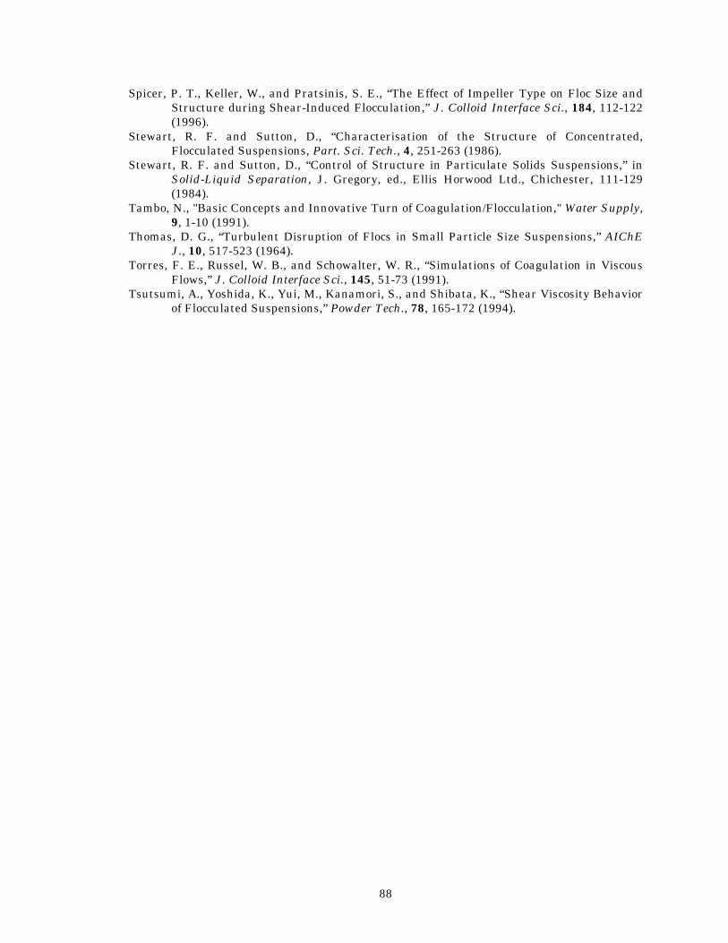
88


Stewart, R. F. and Sutton, D., “Characterisation of the Structure of Concentrated, Flocculated Suspensions, Part. Sci. Tech., 4, 251-263 (1986).

Stewart, R. F. and Sutton, D., “Control of Structure in Particulate Solids Suspensions,” in Solid-Liquid Separation, J. Gregory, ed., Ellis Horwood Ltd., Chichester, 111-129 (1984).



Torres, F. E., Russel, W. B., and Schowalter, W. R., “Simulations of Coagulation in Viscous Flows,” J. Colloid Interface Sci., 145, 51-73 (1991).

Tsutsumi, A., Yoshida, K., Yui, M., Kanamori, S., and Shibata, K., “Shear Viscosity Behavior of Flocculated Suspensions,” Powder Tech., 78, 165-172 (1994).

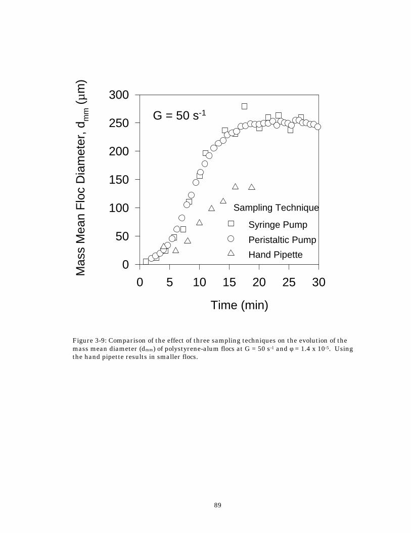
89

Figure 3-9: Comparison of the effect of three sampling techniques on the evolution of the mass mean diameter (dmm) of polystyrene-alum flocs at G = 50 s-1 and φ = 1.4 x 10-5. Using the hand pipette results in smaller flocs.

Time (min)

0 5 10 15 20 25 30

Mas

s M

ean

Flo

c D

iam

eter

, dm

m (

µm)

0

50

100

150

200

250

300

G = 50 s-1

Sampling Technique

Syringe Pump

Peristaltic Pump

Hand Pipette

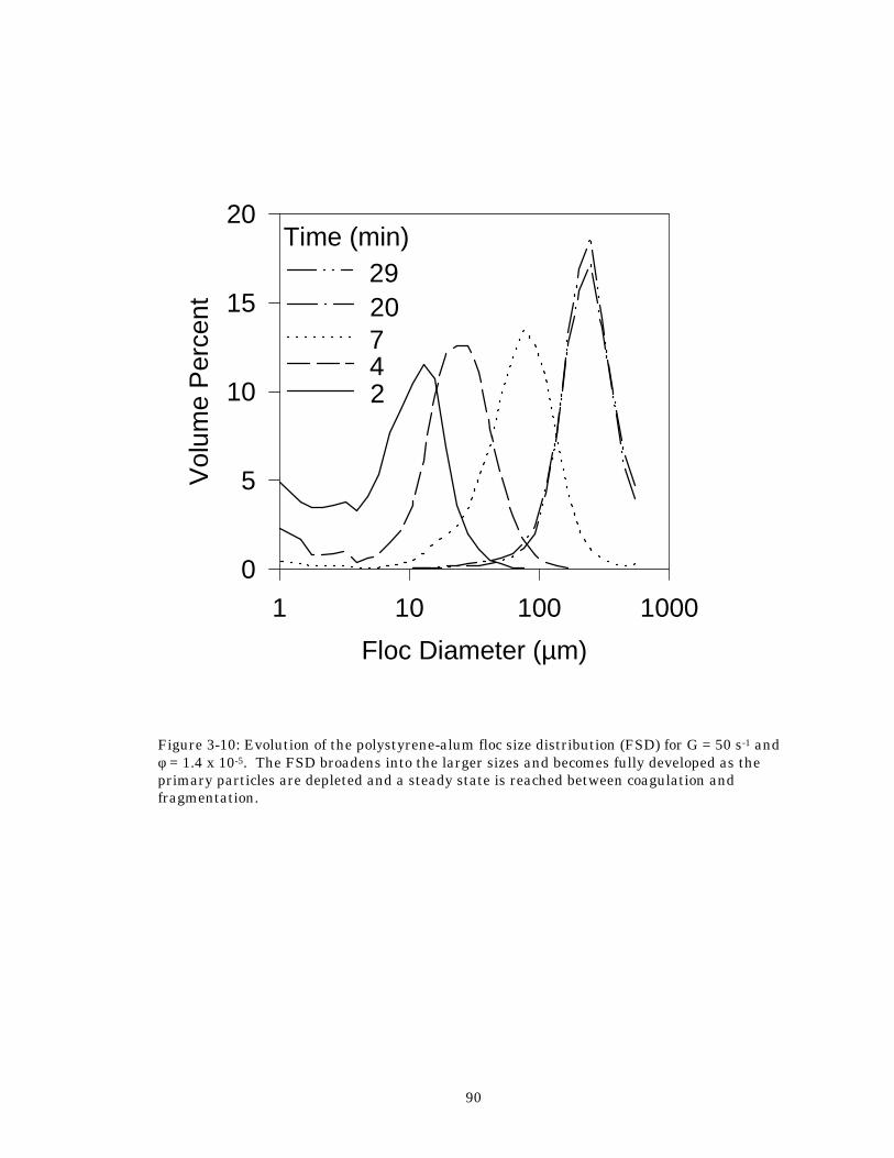
90

Figure 3-10: Evolution of the polystyrene-alum floc size distribution (FSD) for G = 50 s-1 and φ = 1.4 x 10-5. The FSD broadens into the larger sizes and becomes fully developed as the primary particles are depleted and a steady state is reached between coagulation and fragmentation.

Floc Diameter (µm)

1 10 100 1000

Vol

ume

Per

cent

0

5

10

15

20Time (min)

2920742

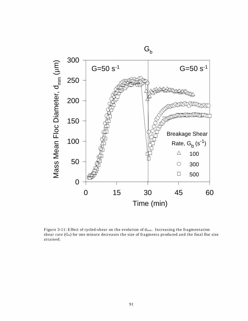
91

Figure 3-11: Effect of cycled-shear on the evolution of dmm. Increasing the fragmentation shear rate (Gb) for one minute decreases the size of fragments produced and the final floc size attained.

Time (min)0 15 30 45 60

Mas

s M

ean

Flo

c D

iam

eter

, dm

m (

µm)

0

50

100

150

200

250

300

Gb

G=50 s-1G=50 s-1

Rate, Gb (s-1)

500

300

100

Breakage Shear

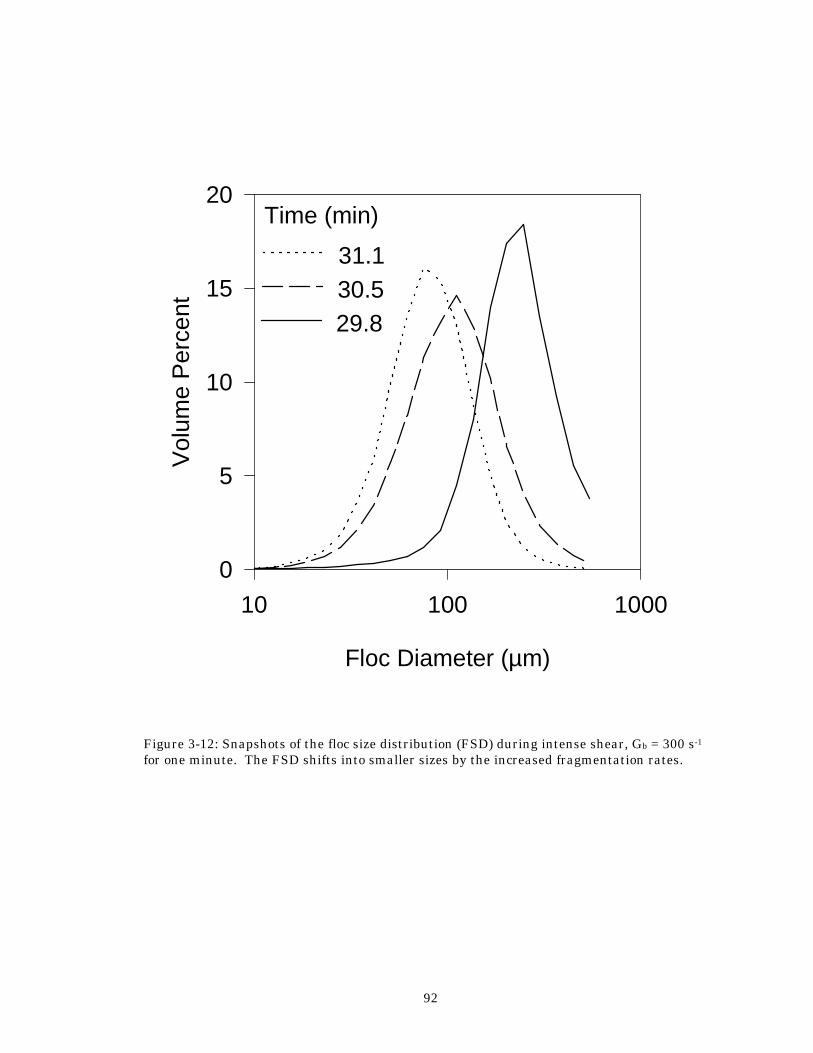
92

Figure 3-12: Snapshots of the floc size distribution (FSD) during intense shear, Gb = 300 s-1 for one minute. The FSD shifts into smaller sizes by the increased fragmentation rates.

Floc Diameter (µm)

10 100 1000

Vol

ume

Per

cent

0

5

10

15

20Time (min)

31.130.529.8

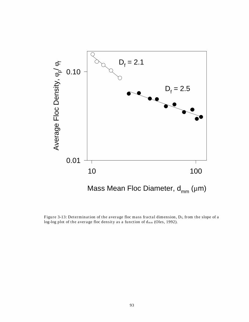
93

Figure 3-13: Determination of the average floc mass fractal dimension, Df, from the slope of a log-log plot of the average floc density as a function of dmm (Oles, 1992).

Mass Mean Floc Diameter, dmm (µm)

10 100

Ave

rage

Flo

c D

ensi

ty, φ

p/ φ

f

0.01

0.10Df = 2.1

Df = 2.5

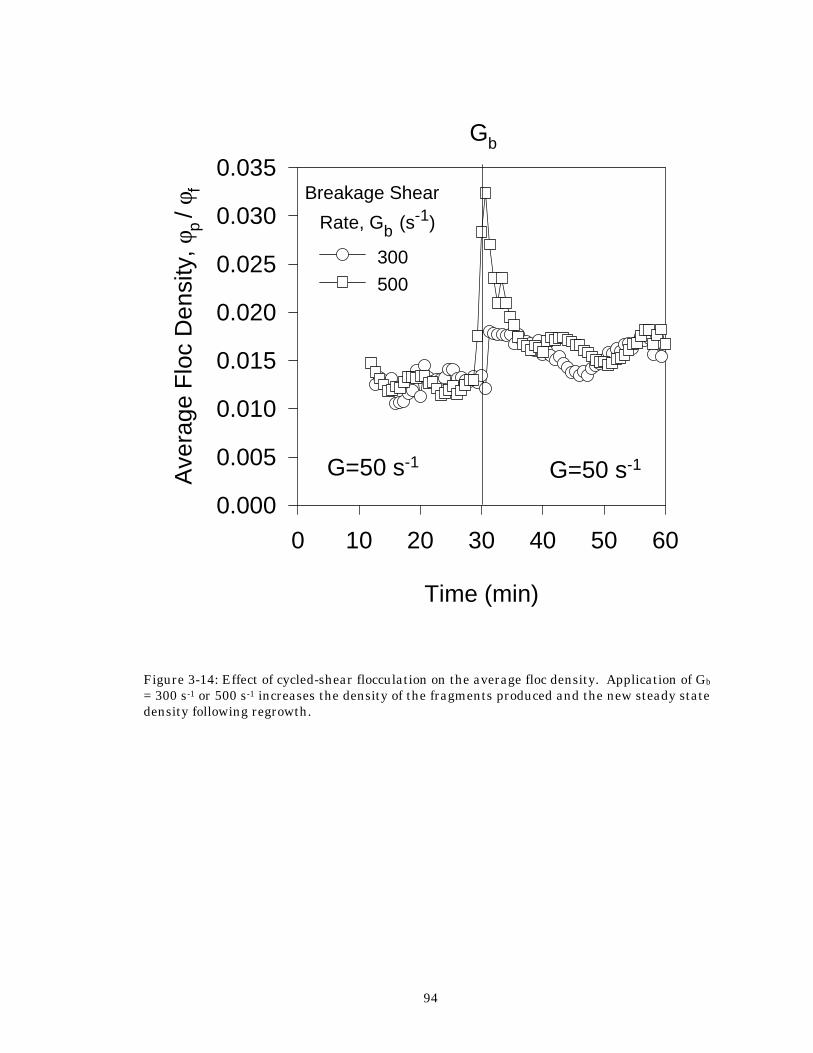
94

Figure 3-14: Effect of cycled-shear flocculation on the average floc density. Application of Gb = 300 s-1 or 500 s-1 increases the density of the fragments produced and the new steady state density following regrowth.

Time (min)

0 10 20 30 40 50 60

Ave

rage

Flo

c D

ensi

ty, φ

p / φ

f

0.000

0.005

0.010

0.015

0.020

0.025

0.030

0.035Gb

G=50 s-1G=50 s-1

Rate, Gb (s-1)

300500

Breakage Shear

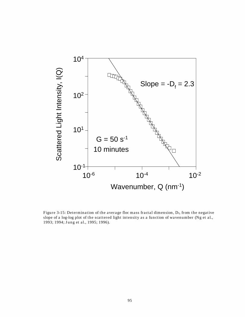
95

Figure 3-15: Determination of the average floc mass fractal dimension, Df, from the negative slope of a log-log plot of the scattered light intensity as a function of wavenumber (Ng et al., 1993; 1994; Jung et al., 1995; 1996).

Wavenumber, Q (nm-1)

Sca

ttere

d Li

ght I

nten

sity

, I(Q

)

G = 50 s-1

Slope = -Df = 2.3

10-6 10-4 10-2

10 minutes

10-1

101

102

104

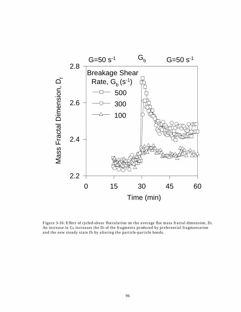
96

Figure 3-16: Effect of cycled-shear flocculation on the average floc mass fractal dimension, Df. An increase in Gb increases the Df of the fragments produced by preferential fragmentation and the new steady state Df by altering the particle-particle bonds.

Time (min)

0 15 30 45 60

Mas

s F

ract

al D

imen

sion

, Df

2.2

2.4

2.6

2.8G=50 s-1 G=50 s-1

Rate, Gb (s-1)

Breakage Shear

Gb

500

300

100

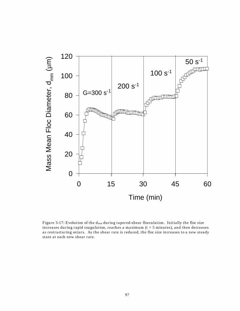
97

Figure 3-17: Evolution of the dmm during tapered-shear flocculation. Initially the floc size increases during rapid coagulation, reaches a maximum (t = 5 minutes), and then decreases as restructuring occurs. As the shear rate is reduced, the floc size increases to a new steady state at each new shear rate.

Time (min)

0 15 30 45 60

Mas

s M

ean

Flo

c D

iam

eter

, dm

m (

µm)

0

20

40

60

80

100

120

100 s-1

200 s-1

G=300 s-1

50 s-1

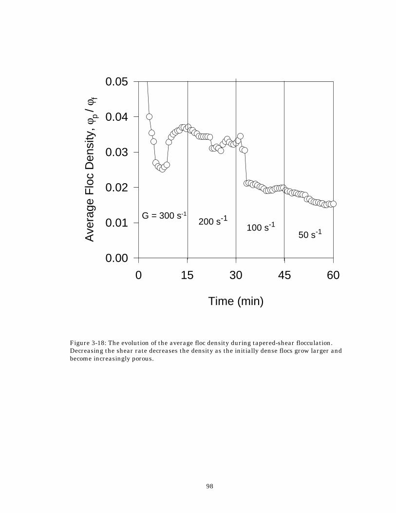
98

Figure 3-18: The evolution of the average floc density during tapered-shear flocculation. Decreasing the shear rate decreases the density as the initially dense flocs grow larger and become increasingly porous.

Time (min)

0 15 30 45 60

Ave

rage

Flo

c D

ensi

ty, φ

p / φ

f

0.00

0.01

0.02

0.03

0.04

0.05

G = 300 s-1

200 s-1100 s-1

50 s-1

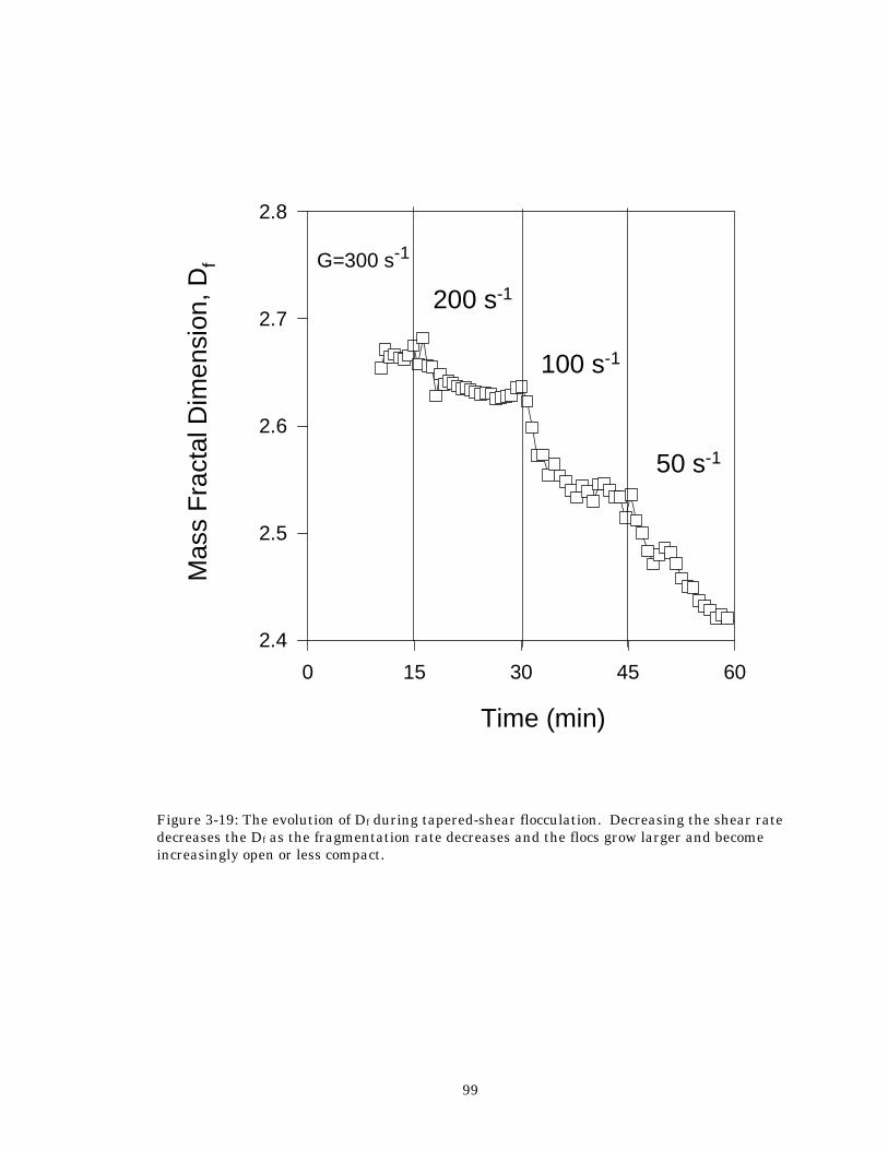
99

Figure 3-19: The evolution of Df during tapered-shear flocculation. Decreasing the shear rate decreases the Df as the fragmentation rate decreases and the flocs grow larger and become increasingly open or less compact.

Time (min)

0 15 30 45 60

Mas

s F

ract

al D

imen

sion

, Df

2.4

2.5

2.6

2.7

2.8

100 s-1

200 s-1

G=300 s-1

50 s-1

100

Chapter 5 - Coagulation and Rotation of Aggregates in Shear Flow Video monitoring of aggregate dynamics in Couette flow is used to determine aggregate rotation rates and compare them with theory for spherical particles. At low shear rates (γ < 3 s-1), the aggregate rotation period increases with increasing radius of gyration. Increasing the shear rate to γ = 3 s-1 decreases the size dependency of the rotation rate near the size-independent spherical limit. Roughly half of the aggregates orient their major axis in the direction of shear flow, while the rest are evenly distributed between 30° and 90° with respect to the flow direction. The average aggregate structure is characterized by a mass fractal dimension of Df = 1.8, consistent with shear-induced aggregation theory and experiment. The effects of rotation and orientation on the collision area of aggregates are compared with simulated fractal aggregates (Df = 1.5 - 2.5). It is shown that assuming a fractal collision rate based on maximum aggregate radius over estimates the shear-induced coagulation rate. Aggregate collision area is shown to vary as a result of aggregate orientation and rotation.

101

Introduction When fluid shear is applied to a suspension of solid particles, different types of fluid-

particle and particle-particle interactions alter the microscopic and macroscopic characteristics of the suspension. In the absence of repulsive particle-particle interactions, shear-induced velocity gradients bring about particle-particle collisions (coagulation) that increase the average particle size and decrease the total particle number concentration. As a result, the rate of particle collisions determines the evolution of the microscopic particle size distribution and affects the macroscopic suspension properties (i.e. viscosity).

The instantaneous cross-sectional area of two colliding particles determines the shear-induced binary particle collision rates, a result derived by Smoluchowski (1917) for laminar shear flow and by Saffman and Turner (1956) for isotropic turbulent flow. While the collision rates of spherical particles are easily calculated, practical systems often contain irregular, non-spherical aggregates that can behave quite differently from their spherical counterparts (Oles, 1992; Kusters et al., 1996). Current aggregate collision rate theory is based on collisions of spheres (Smoluchowski, 1917; Saffman and Turner, 1956) and assumes that aggregates possess a cross-sectional area equal to that of a “collision sphere” completely enclosing the aggregate. The size of the collision sphere can then be calculated by assuming the aggregates possess a fractal structure and are “fractal-like” (Jiang and Logan, 1991; Wiesner, 1992). However, this description can overestimate collision rates because an aggregate’s anisotropic structure is approximated by a space filling sphere, which ignores the inherent aggregate porosity. In addition, aggregate cross-sectional area calculations are not straightforward as there is substantial uncertainty in expressions for the linear dimensions of fractal aggregates (Neimark et al., 1996). Finally, the aggregate collision area is also a function of orientation, which is in turn a function of shear-induced particle rotation.

By definition of fluid vorticity, spherical particles rotate at half the simple shear rate applied to a particle suspension, a phenomenon confirmed experimentally in laminar flow (Trevelyan and Mason, 1951) and turbulent flow (Ye and Roco, 1992) that can enhance a suspension’s thermal conductivity (Wang et al., 1989). Shear-induced rotation of spherical particles may form closed streamlines around particles, hindering the approach of other particles with insufficient inertia, thus reducing the shear-induced particle collision rate (Greene et al., 1994; Brunk et al., 1997). Little is known about shear-induced rotation of irregular particles, although Jeffery (1922) derived the rotation rate of ellipsoids. Trevelyan and Mason (1951) were unable to apply this theory to cylindrical fibers. The rotational behavior of aggregates is not well characterized, and is often assumed to follow that of spherical particles (Torres et al., 1991). However, as an aggregate rotates about its center of mass, distinct variations in the cross-sectional area at a given moment may occur, significantly influencing aggregation kinetics and other transport properties.

Simulation of evolving suspension transport properties and particle size distributions requires increasingly accurate knowledge of particle-particle and particle-fluid interactions. Nevertheless, the assumption of spherical or pseudo-spherical properties for anisotropic aggregates is convenient for simulations of particle coagulation and suspension viscosity (Doi and Chen, 1989; Potanin, 1991; 1992), for lack of quantitative data on anisotropic aggregate behavior in shear flow. The objective of this study is to contribute to an understanding of the dynamics of suspended aggregates in simple shear flow and compare them that of spherical particles. The rotation rate and collision profile of fractal-like aggregates are determined experimentally by a unique image analysis technique that provides a full 360° view of aggregates in shear flow. The rotational behavior of the fractal-like aggregates is compared with that of spheres in shear flow. In addition, simulated fractal aggregates covering a wide range of structures are used to characterize the collision profile of aggregates. These results are compared with experimental and theoretical data in the literature to evaluate the accuracy of the “collision sphere” approach to describe the collision rate of aggregates.

102

Theory

Shear-Induced Particle Rotation and Collision Spherical particles in laminar shear flow exhibit rotational motion in the direction of

travel with a constant angular velocity ω (Vand, 1948):

ωγ

=2

(5-1)

and a period of rotation τ:

τπγ

=4

(5-2)

Equations (5-1) and (5-2) assume suspended particles that follow the bulk fluid vorticity and were confirmed experimentally by Trevelyan and Mason (1951).

Smoluchowski (1917) developed an expression for the collision rate of two spheres i and j based on the velocity gradient, γ, experienced in simple shear flow:

( )β γi j i ja a, = +43

3 (5-3)

where ai is the radius of particle i. Aggregates of spheres are less straightforward to describe. The mass, M, of self-

similar, irregular fractal objects scales with an object’s linear dimension, L, as (Mandelbrot, 1987):

M LD f∝ (5-4)

where Df is the mass fractal dimension of the object and varies from 1 to 3 with increasing compactness of the object structure. The radius of gyration, Rg, of an aggregate of i primary particles with radius a follows a similar scaling law (Jullien and Botet, 1987):

i kR

agg

D f

=

(5-5)

as does its collision radius, Rc, the radius of a sphere completely enclosing the aggregate:

i kRac

cD f

=

(5-6)

In Equations (5-5) and (5-6) kg and kc are proportionality constants, lacunarities. The two aggregate dimensions are related by (Rogak and Flagan, 1990):

R RD

Dc gf

f

=+

21

2

(5-7)

Equation (5-3) is often used to describe aggregate collision rates by use of Equation (5-6) (Jiang and Logan, 1991; Kusters, 1991):

β γi j cD D Dk a i jf f f

, = +

−43

3

3

1 1 3

(5-8)

103

where i and j are the number of primary particles in each aggregate. When Df = 3 (spherical particles) Equation (5-8) reduces to Equation (5-3). The proportionality constant, kc, in Equation (5-8) is often assumed to be equal to one so as to be consistent with the limiting case of a zero porosity primary particle (Cohen and Wiesner, 1990). Calculations using kc = 1 have been used to model the early stages of shear-induced aggregation (Jiang and Logan, 1991; Wiesner, 1992) but the exact value is not known (Sorensen and Roberts, 1997). Various values have been reported based on experimental results for a single fractal dimension (Torres et al., 1991; Neimark et al., 1996) or theoretical studies over a narrow range of Df (Sorensen and Roberts, 1997).

The overestimation of the aggregate collision area by the collision sphere concept introduces additional uncertainty into the description of fractal aggregate kinetics. Equation (5-8) can thus be thought of as the maximum aggregate collision rate. A more accurate description must rely on the actual aggregate “collision area” versus a spherical equivalent value based on the maximum aggregate length. The cross-sectional area of an aggregate, σ, presented to an oncoming aggregate determines the likelihood of a collision between the two. Meakin et al. (1989) examined model aggregates with Df = 1.8, 1.95, 2.09, and 2.12 and found that σ scaled with the number of primary particles in the aggregate as:

σ ∝ i (5-9)

when Df ≤ 2 and

σ ∝ iD f

2

(5-10)

when Df > 2. As these previous studies have largely been concerned with aerosol dynamics, aggregate rotation has been ignored and a rather narrow range of aggregate fractal dimensions has been studied. As a result, it will be helpful to examine a broader range of aggregate structures and determine the effect of aggregate orientation on collision area.

Simulated Fractal Aggregates Model aggregates were constructed using the hierarchical cluster-cluster aggregation (CCA) algorithm of Thouy and Jullien (1994) to produce aggregates with a specified fractal dimension, Df between 1.5 and 2.5. The algorithm starts with an initial number of primary particles, i = 2n on a cubic lattice. Then, at every jth iteration, particle/aggregate pairs are chosen to collide until j = n and only one aggregate remains. During a collision event, all possible non-overlapping positions of the colliding aggregate relative to the reference aggregate are examined and the distance between the aggregates’ centers of mass (COM) is calculated. This distance is then compared to the desired value, Γ :

Γ = k Rgi2 (5-11)

where <Rgi2 > is the mean square radius of gyration of an aggregate of i particles, and k is a proportionality constant (Thouy and Jullien, 1994):

k = −2 4 11

∆ (5-12)

and ∆ is the desired fractal dimension. The pairing that best matches the desired structure is used or, when several positions match, one is chosen randomly. The algorithm works if Df = ∆. An estimate of Df, D(i), was calculated at each iteration as an accuracy monitor (Thouy and Jullien, 1994):

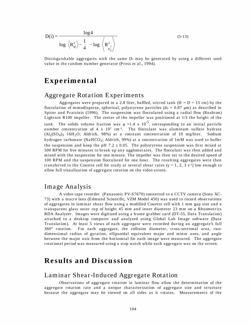
104

D i

R Rgig

i

( )log

log log

=

−

−

4

14

2

2

2

(5-13)

Distinguishable aggregates with the same Df may be generated by using a different seed value in the random number generator (Press et al., 1994).

Experimental

Aggregate Rotation Experiments Aggregates were prepared in a 2.8 liter, baffled, stirred tank (H = D = 15 cm) by the

flocculation of monodisperse, spherical, polystyrene particles (d0 = 0.87 µm) as described in Spicer and Pratsinis (1996). The suspension was flocculated using a radial flow (Rushton) Lightnin R100 impeller. The center of the impeller was positioned at 1/3 the height of the

tank. The solids volume fraction was φ =1.4 x 10-5, corresponding to an initial particle number concentration of 4 x 107 cm-3. The flocculant was aluminum sulfate hydrate (Al2(SO4)3 16H2O; Aldrich, 98%) at a constant concentration of 10 mg/liter. Sodium hydrogen carbonate (NaHCO3; Aldrich, 99%) at a concentration of 1mM was used to buffer the suspension and keep the pH 7.2 ± 0.05. The polystyrene suspension was first mixed at 500 RPM for five minutes to break up any agglomerates. The flocculant was then added and mixed with the suspension for one minute. The impeller was then set to the desired speed of 100 RPM and the suspension flocculated for one hour. The resulting aggregates were then transferred to the Couette cell for study at several shear rates (γ = 1, 2, 3 s-1) low enough to allow full visualization of aggregate rotation on the video screen.

Image Analysis A video tape recorder (Panasonic PV-S7670) connected to a CCTV camera (Sony XC-

73) with a macro lens (Edmund Scientific, VZM Model 450) was used to record observations of aggregates in laminar shear flow using a modified Couette cell with 1 mm gap size and a transparent glass outer cup of height 45 mm and inner diameter 23 mm on a Rheometrics RDA Analyzer. Images were digitized using a frame grabber card (DT-55, Data Translation) attached to a desktop computer and analyzed using Global Lab Image software (Data Translation). At least 5 views of each aggregate were recorded during an aggregate’s full 360° rotation. For each aggregate, the collision diameter, cross-sectional area, two-dimensional radius of gyration, ellipsoidal equivalent major and minor axes, and angle between the major axis from the horizontal for each image were measured. The aggregate rotational period was measured using a stop watch while each aggregate was on the screen.


Laminar Shear-Induced Aggregate Rotation Observations of aggregate rotation in laminar flow allow the determination of the

aggregate rotation rate and a unique characterization of aggregate size and structure because the aggregate may be viewed on all sides as it rotates. Measurements of the

105

aggregate rotation period, τ, are shown in Figure 5-1 for three shear rates (γ = 1, 2, 3 s-1) along with the best-fit lines as a function of the three-dimensional aggregate radius of gyration, Rg. The Rg is obtained by averaging the two dimensional radius of gyration over all successive images of the aggregate as it rotates. Several measurements of τ were made for each aggregate and then averaged. The reproducibility error was less than 0.5%.

In Figure 5-1, at γ = 1 s-1, the aggregate rotation period increases with increasing aggregate size, varying between τ = 5 -10 seconds. For spheres, however, at γ = 1 s-1 the calculated rotation period is constant at τ = 4π seconds (Equation (5-2)). By definition as fractal structures, aggregates become more openly structured and porous as their size increases (Meakin, 1988). The aggregate structure is expected to increase the amount of surface drag on the aggregate relative to a uniform sphere (Rogak and Flagan, 1990), thus increasing the rate of fluid vorticity-induced rotation. In addition, aggregate porosity allows flow through the structure (Adler, 1981; Chellam and Wiesner, 1993; Veerapaneeni and Wiesner, 1996), further reducing fluid resistance to rotation. As a result, at γ = 1 s-1 the aggregates rotate more rapidly than spheres as a result of fluid drag resulting in the observed size dependency.

As the shear rate is increased from 1 s-1 to 2 s-1, the rotation period becomes nearly independent of aggregate size (Figure 5-1). At γ = 2 s-1, the rotation period is nearly constant at τ = 4 seconds and smaller than that of 2π (seconds) for spherical particles from Equation (5-2). The size dependency observed for γ = 1 s-1 may disappear at higher shear rates as fluid is trapped in the void spaces of the aggregate and a nearly spherical entity is formed that rotates much like a sphere independent of its size. The fluid-aggregate body rotates more rapidly than solid spheres, possibly because of the smaller amount of solid area available to resist rotation. Finally, increasing the shear rate further to γ = 3 s-1 further increases the rotation rate to a constant period of τ = 2.8 seconds, smaller than the spherical equivalent of τ = 4π / 3 given by Equation (5-2) (Figure 5-1). Increasing the shear rate increases the rotation rate of the aggregates and gradually removes its size dependency. The assumption of a constant rotation rate for aggregates is apparently valid at sufficiently high shear rates. Applying the theory for spherical particles to aggregates over estimates the aggregate rotation rate for the conditions examined here.

The shear dynamics of aggregates are also influenced by their orientation with respect to the direction of fluid flow. It is possible to estimate the distribution of aggregate orientations from the statistics of the aggregates analyzed above. Comparisons of the distribution of the angle, θ, between the aggregate major axis and the horizontal (direction of flow) were made for all three shear rates. At each shear rate, roughly 50% of the aggregate major axes are aligned parallel to the fluid flow (0-30°). This fraction increases from 48% to 56% with increasing shear rate. The rest were evenly distributed between 30° and 90° (perpendicular to the fluid flow direction). The orientation of an aggregate determines its collision profile as it approaches or is approached by another aggregate in shear flow. The aggregate orientation can influence the sizing of aggregate as a result of its anisotropic structure.

Three-Dimensional Image Analysis Characterization of Polystyrene-Alum Aggregates Shear-induced aggregate rotation provides an excellent basis for aggregate characterization by affording a full 360° view of aggregates as they simultaneously rotate and move across the field of view. This is in contrast to standard two-dimensional microscopy that views the aggregate in only one orientation. By characterizing several aggregate orientations, a more accurate assessment of aggregate size and morphology is attained. Figure 5-2 shows the (maximum over all orientations) collision radius, Rc, of polystyrene-alum aggregates as a function of the 3-D radius of gyration (averaged over

106

several measurements of the 2-D radius of gyration), Rg for all three shear rates. By definition, Rc, the maximum radius of the aggregate, will grow faster than Rg, the three dimensional average of the distance of all particles in the aggregate from the COM. As a result, Equation (5-7) can be used to estimate the aggregate fractal dimension, Df, in order to characterize the experimental suspension.

In Figure 5-2, Rc is calculated from Equation (5-7) and a range of Rc are plotted for Df = 1.5 – 2.5 and compared with the experimental data. A linear regression gives Df = 1.8 ± 0.1, in excellent agreement with Torres et al. (1991) who found Df = 1.8 for aggregates formed by experimental and simulated laminar shear coagulation. However, the scatter in Figure 2 emphasizes the fact that there is a distribution of aggregate structures produced in a shear field as a result of the complex interactions of coagulation and possibly restructuring processes. An average Df = 1.8 is low when compared to high shear laminar (Oles, 1992) and turbulent shear-produced aggregates that experience fragmentation and restructuring (Kusters et al., 1996). The aggregates may mostly coagulate when sheared in the Couette cell, leading to more open structures at the employed shear rates. Assuming the validity of Equation (5-7), the size and structure of suspended aggregates may be characterized by the three-dimensional rotational image analysis technique. These three-dimensional aggregate views can also be used to evaluate the linear dimension that best characterizes aggregate collision dynamics. Figure 5-3 compares the aggregate collision area calculated using the collision sphere assumption (A = π r2) for r = Rg and r = Rc with the aggregate area averaged over all recorded orientations. In Figure 5-3 the calculated Rc-based area exceeds that of the experimentally measured values for all three shear rates, while the Rg-based calculation is quite close to experiment. The Rg appears to provide the best estimate of aggregate characteristics for calculating aggregation rates. No exact analytical expression exists for the calculation of an aggregate Rg because of the inherently random structure of fractal aggregates. Equation (5-5), however, offers a means of estimating Rg as a function of aggregate mass and fractal dimension, provided the correct coefficients are utilized. Determination of these parameters from simulated aggregates allows a systematic study of aggregate properties.

Characterization of Simulated Fractal Aggregates In order to explore the effect of aggregate structure on aggregation kinetics, model

aggregates were constructed with a range of Df values (1.5, 1.7, 1.9, 2.1, 2.3, 2.5). The algorithm was validated by calculation of the aggregate fractal dimension at each iteration using Equation (5-13) (Thouy and Jullien, 1994). For all runs, the calculated value of D(i) matched the specified ∆ within 0.1 percent after the fourth iteration (i = 16), in excellent agreement with Thouy and Jullien (1994) for ∆ = 1.5 - 2.5. Equation (5-13) only provides an estimate of Df. The Df values of the simulated aggregates were determined from a log-log plot of the number of primary particles in an aggregate as a function of the average aggregate radius of gyration at each hierarchical step of the algorithm. Such plots were linear, with a correlation coefficient exceeding r2 = 0.998, emphasizing the fractal nature of the aggregates, although the Df determined from the slope of the best fit line does not exactly match the specified ∆. In all cases the D(i) slightly overestimated the actual Df and the correlation of the two parameters was used to prepare aggregates with the desired Df. The study of cluster-cluster aggregates is equally applicable to the behavior of aggregates formed in aerosol (Oh and Sorensen, 1997) and suspension processes (Torres et al., 1991) and the flexible algorithm used here permits precise study of aggregate characteristics over a wide range of fractal structures.

Figure 5-4 shows three-dimensional renderings of six simulated aggregates of 256 particles over the entire Df range examined here. Increasing the Df clearly results in a transition to more compact, space-filling structures and a resultant decreased collision

107

profile. At low Df (1.5 - 1.7) the porosity of the aggregates is such that one can imagine an approaching particle passing through the aggregate structure, while at higher Df the structures are more compact. Figure 5-4 also emphasizes the variation in collision area expected as a fractal aggregate rotates about its center of mass. For Df = 1.5, the variation in area could be quite large as an aggregate rotates so that its major axis confronted the viewer end on.

Coagulation Rate Expression Effects Shear-induced rotation will continuously vary an aggregate’s cross-sectional collision area, thus varying the probability of collision with other approaching aggregates. In addition, aggregates may orient parallel with or perpendicular to the direction of shear flow, creating additional variations. The variation of aggregate area at various orientations was calculated following aggregate generation. Aggregates are oriented with their major axis either along the z- (perpendicular) or x-axis (parallel) and rotated around their COM with flow assumed to be in the positive x direction. These two extreme cases represent rotation of an aggregate on its major axis (perpendicular) or end over end along its major axis (parallel). Instantaneous areas are then calculated at each orientation as a projection on the y-z plane. This approach will slightly underestimate collision area by ignoring potential small holes in the aggregate that are completely enclosed by particles, while these holes would not always allow an approaching particle to pass without collision. This error is only expected at low Df and thus more open aggregate structures, at higher Df the aggregates are expected to be opaque.

Figure 5-5 shows the variation in the cross-sectional area of simulated aggregates of 1024 primary particles with a = 1 as a function of Df as they are rotated a full 360° while oriented with their major axes either a) parallel or b) perpendicular to the flow (and thus other aggregates). As Df increases, the aggregates become more compact, decreasing the average aggregate area for both orientations. A distinct oscillation in the aggregate area with rotation is noticeable in both orientations, in some cases by as much as 20%. The area variations of aggregates oriented parallel to the flow direction are less frequent but higher in magnitude than for perpendicular orientation. The extent of variation in aggregate area is relatively independent of Df, with no clear trend evident at either orientation. The area minimums observed in Figure 5-5 are caused as the aggregate is viewed end-on and has a much smaller collision profile than in other orientations that display the entire aggregate length. The more frequent area variations for the perpendicular orientation may be caused by variations in the aggregate width, a dimension that needs to be characterized along with the aggregate length (Mandelbrot, 1987; Neimark et al. 1996). However, Figure 5-5 emphasizes the variation in both of these dimensions with orientation and the need for caution when characterizing aggregates using two dimensional projections alone. By averaging the aggregate area over all orientations, an estimate of the collision profile can be determined as a function of Df.

Figure 5-6 compares the average aggregate cross-sectional area, A, of aggregates with a range of Df with the area calculated from the aggregate collision radius, Ac and radius of gyration, Ag. The spherical volume equivalent area of As = π i2/3 d02/ 4 = 80 significantly underestimates the aggregate area for all Df, indicating the need to account for aggregate collision kinetic enhancement by the aggregate structures. As noted earlier, Ac estimates the maximum aggregate collision area because of its pseudo-spherical premise. In Figure 5-6, the Ac overestimates the actual aggregate area by more than an order of magnitude for very open aggregates (Df ≤ 1.7). As Df increases and the aggregate structure becomes more compact (approaching sphericity), the Ac is in better agreement with the measured aggregate area (circles). However, while the value of Ag more closely approximates the average aggregate area, it over predicts A at Df < 1.7 and under predicts A at Df >1.7. It is interesting to note that the best agreement between A and Ag is around Df = 1.7 – 1.8, supporting the

108

value of Df = 1.8 determined from Figure 5-2 and the agreement between A and Ag found experimentally in Figure 5-3. As a result, Equation (5-8) must be used with caution to simulate aggregate collision dynamics as an improper choice of a characteristic dimension can introduce significant error. The accurate calculation of aggregate collision areas may be complicated further by the lack of certainty in the proportionality constants in Equations (5-5) and (5-6).

Log-log plots of i versus Rg and Rc respectively allow the determination of the proportionality constants in Equations (5-5) and (5-6) as a function of Df by examining the structure of aggregates with a range of Df . Figure 5-7a shows the variation in the Rg-based lacunarity, kg, of the simulated aggregates as a function of Df and compares the simulation results with theoretical (Chen and Doi, 1989; Potanin, 1993; Sorensen and Roberts, 1997) and experimental (Koylu et al., 1995; Johnson et al., 1996) aggregation data. The advantage of examining aggregates over a broad range of Df is immediately apparent: a discontinuity in kg is observed at Df = 2 that would not be distinguishable from numerical variation in a narrower range of data. This discontinuity is consistent with the transition from a transparent to a more complex structure for fractal aggregates at Df = 2 (Meakin et al., 1989). Increasing Df clearly decreases kg, but there appear to be two linear regions divided by the transition point at Df = 2.

The experimental data of Koylu et al. (1995) and Johnson et al. (1996) are significantly larger than the results calculated for the simulated aggregates of this study, in agreement with Neimark et al. (1996). However, there appears to be a discontinuity at Df = 2 for the experimental data as well, although it is difficult to be certain since these data are for completely different experimental systems (aerosol and suspension, respectively). When compared to the results of other simulations, the results of this study are slightly higher than those of Sorensen and Roberts (1997) for Df > 2, possibly because they examined aggregates of only 10-100 particles. The simulations of Chen and Doi (1989) were performed assuming aggregate breakage and restructuring occur, producing a result that exceeds the values of this study. The most interesting comparison is with the simulation results of Potanin (1993), who specifically examined the effects of fluid shear on model aggregates by simulating their fragmentation by stretching. Not only do these simulation results exceed the values of the current study, but they are in excellent agreement with the experimental data of Johnson et al. (1996), who documented the occurrence of aggregate breakage and restructuring. The results in Figure 5-7a indicate that a possible explanation for the under estimation of lacunarity data by simulation is the lack of restructuring information in most theoretical simulations. Aggregates formed in aerosol processes can restructure by sintering, while suspension aggregates can restructure by fragmentation and regrowth, in each case producing more compact structures. The link between the lacunarity and the aggregate packing density, (Kusters et al., 1996; Sorensen and Roberts, 1997), may also lend support to the above hypothesis, indicating the need for future simulation studies to incorporate realistic aggregation and restructuring algorithms. Jullien and Meakin (1989) found more compact structures (increased Df) with the incorporation of restructuring algorithms into cluster-cluster simulations, but did not treat lacunarity variations.

Figure 5-7b shows a similar comparison of theoretical and experimental lacunarity data based on the aggregate collision radius. The variation of kc with Df is similar to that observed for kg, a discontinuity at Df = 2 is present and a trend of decreasing kc with increasing Df is also seen. The experimental data of Torres et al. (1991) were obtained for laminar shear-induced aggregation but are relatively close to the simulation results. The data of Kusters et al. (1996), however, were obtained for turbulent shear-induced aggregation in a stirred tank, where aggregate breakage and restructuring may occur more frequently in the non-uniform flow. As a result, the more intense turbulent restructuring processes may explain the larger discrepancy between the simulation results and those of Kusters et al. (1996) relative to the comparison with Torres et al. (1991), although more data are required. This conclusion is, however, also consistent with the supposition that the lacunarity

109

parameters are indicative of aggregate packing densities (Kusters et al., 1996; Sorensen and Roberts, 1997). Aggregates restructure to more compact configurations, leading to increased packing density relative to simulation results.

The finding that lacunarity data are much higher than previously thought indicates that previous practical estimates of fractal aggregate maximum linear dimensions have been over estimated, as have aggregate collision rates (Equation (5-8)). The results of this study indicate that the aggregate radius of gyration may more accurately characterize aggregate collision profiles, but such calculations require results from simulations incorporating restructuring phenomena or a broad range of experimental data.

Conclusions A new approach to image analysis characterization of aggregates in shear flow has been developed that allows for a three-dimensional view of aggregates and thus a more accurate structural representation. The rotation rate of aggregates is shown to approach that of spherical particles as the shear rate is increased from 1 s-1 to 3 s-1. The image analysis technique is applied to determine the collision area of aggregates relative to the value calculated by theory based on the aggregate maximum dimension, a theory shown to significantly over predict aggregate collision areas and thus collision kinetics. Simulated cluster-cluster aggregates are used to characterize aggregate collision dynamics over a range of fractal dimensions. Aggregate collision area is shown to vary as a result of aggregate orientation.

Acknowledgments We acknowledge the financial support of Genencor International and discussions with Prof. G. G. Lipscomb (University of Toledo, Toledo, Ohio).

110

Notation 2D two dimensional 3D three dimensional a particle radius (µm) A orientation-averaged aggregate cross-sectional area (unit2) Ac aggregate cross-sectional area calculated from πRc2 (unit2) Ag aggregate cross-sectional area calculated from πRg2 (unit2) COM center of mass (-) d0 primary particle diameter (µm) D stirred tank diameter (cm) Df mass fractal dimension (-) D(i) approximate fractal dimension (-) G average turbulent shear rate (s-1) H stirred tank height (cm) i number of primary particles in an aggregate (-) k proportionality constant used to calculate aggregate simulation parameters (-) kg lacunarity of mass scaling with aggregate radius of gyration (-) kc lacunarity of mass scaling with aggregate collision radius (-) L characteristic length of aggregate (µm) M mass of an aggregate (g) r2 correlation coefficient (-) Rc aggregate collision radius (µm) Rg aggregate radius of gyration (µm)

Greek Letters

β shear-induced collision rate (cm3 / s) γ shear rate (s-1) Γ distance between two aggregate centers of mass (unit) ∆ specified fractal dimension (-) φ solids volume fraction (-) τ aggregate rotation period (s) θ angle of rotation (degrees)

111

References Adler, P. M., “Streamlines in and Around Porous Particles,” J. Colloid Interface Sci., 81, 531-

535 (1981). Brunk, B. K., Koch, D. L., and Lion, L. W., “Turbulent Coagulation of Particles Smaller than

the Kolmogorov Length Scale,” submitted to J. Fluid Mechanics, (1997). Chellam, S. and Wiesner, M. R., “Fluid Mechanics and Fractal Aggregates,” Wat. Res., 27,

1493-1496 (1993). Cohen R. D. and Wiesner, M. R., “Equilibrium Structure and the Kinetics of Fractal

Aggregation,” J. Surface Sci. Technol., 6, 25-46 (1990). Doi, M. and Chen, D., “Simulation of Aggregating Colloids in Shear Flow,” J. Chem. Phys.,

90, 5271-5279 (1989). Greene, M. R., Hammer, D. A., and Olbricht, W. L., “The Effect of Hydrodynamic Flow Field

on Colloidal Stability,” J. Colloid Interface Sci., 167, 232-246 (1994). Jeffery, G. B., “The Motion of Ellipsoid Particles Immersed in a Viscous Fluid,” Proc. Roy.

Soc. London, A102, 161-179 (1922). Jiang and Logan, B. E., “Fractal Dimensions of Aggregates Determined from Steady State

Size Distributions,” Env. Sci. and Tech., 25, 2031-2038 (1991). Johnson, C. P., Li, X., and Logan, B. E., “Settling Velocities of Fractal Aggregates,” Env. Sci.

Tech., 30, 1911-1918 (1996). Jullien, R. and Botet, R., Aggregation and Fractal Aggregates, World Scientific, Singapore,

(1987). Jullien, R. and Meakin, P., “Simple Models for the Restructuring of Three-Dimensional

Ballistic Aggregates,” J. Colloid Interface Sci., 127, 265-272 (1989). Krutzer, L. L. M., Van Diemen, A. J. G., and Stein, H. N., “The Influence of the Type of Flow

on the Orthokinetic Coagulation Rate,” J. Colloid Interface Sci., 171, 429-438 (1995). Kusters, K. A., Wijers, J. G., and Thoenes, D., “Aggregation Kinetics of Small Particles in

Agitated Vessels,” Chem. Eng. Sci., 52, 107-121 (1996). Mandelbrot, B. B., The Fractal Geometry of Nature, W. H. Freeman and Company, New

York, (1987). Meakin, P., "Fractal Aggregates," Adv. Colloid Interface Sci., 28, 249-331 (1988). Meakin, P., Donn, B., and Mulholland, G. W., “Collisions between Point Masses and Fractal

Aggregates,” Langmuir, 5, 510-518 (1989). Neimark, A. V., Koylu, U. O., and Rosner, D. E., “Extended Characterization of Combustion-

Generated Aggregates: Self-Affinity and Lacunarities,” J. Colloid Interface Sci., 180, 590 (1996).

Oh, C. and Sorensen, C.M., “Light Scattering Study Of Fractal Cluster Aggregation Near The Free Molecular Regime,” J. Aerosol Sci., 28, 937 (1997).


Potanin, A. A., “On the Mechanism of Aggregation in the Shear Flow of Suspensions,” J. Colloid Interface Sci., 145, 140-157 (1991).

Potanin, A. A., “On the Model of Colloid Aggregates and Aggregating Colloids,” J. Chem. Phys., 96, 9191-9200 (1992).

Press, W. H., Teukolsky, S. A., Vetterling, W. T., & Flannery, B. P. Numerical Recipes in FORTRAN, 2nd Ed. Cambridge, New York, 271 (1994).

Rogak, S. N. and Flagan, R. C., “Stokes Drag on Self-Similar Clusters of Spheres,” J. Colloid Interface Sci., 134, 206-218 (1990).


Smoluchowski, M., “Versuch Einer Mathematischen Theorie de Koagulations- Kinetic Kolloider Losungen,” Z. Phys. Chem., 92, 129-168 (1917).

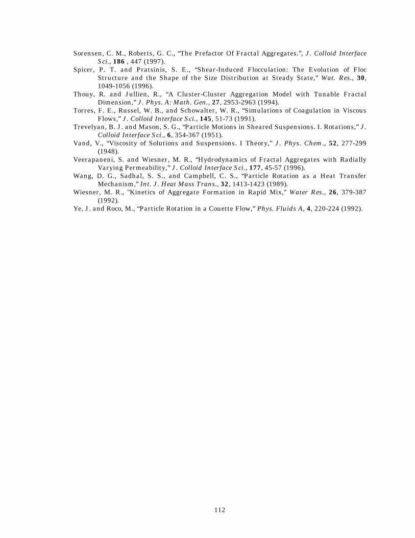
112

Sorensen, C. M., Roberts, G. C., “The Prefactor Of Fractal Aggregates.”, J. Colloid Interface Sci., 186 , 447 (1997).


Thouy, R. and Jullien, R., “A Cluster-Cluster Aggregation Model with Tunable Fractal Dimension,” J. Phys. A: Math. Gen., 27, 2953-2963 (1994).


Trevelyan, B. J. and Mason, S. G., “Particle Motions in Sheared Suspensions. I. Rotations,” J. Colloid Interface Sci., 6, 354-367 (1951).

Vand, V., “Viscosity of Solutions and Suspensions. I Theory,” J. Phys. Chem., 52, 277-299 (1948).

Veerapaneni, S. and Wiesner, M. R., “Hydrodynamics of Fractal Aggregates with Radially Varying Permeability,” J. Colloid Interface Sci., 177, 45-57 (1996).

Wang, D. G., Sadhal, S. S., and Campbell, C. S., “Particle Rotation as a Heat Transfer Mechanism,” Int. J. Heat Mass Trans., 32, 1413-1423 (1989).

Wiesner, M. R., "Kinetics of Aggregate Formation in Rapid Mix," Water Res., 26, 379-387 (1992).

Ye, J. and Roco, M., “Particle Rotation in a Couette Flow,” Phys. Fluids A, 4, 220-224 (1992).

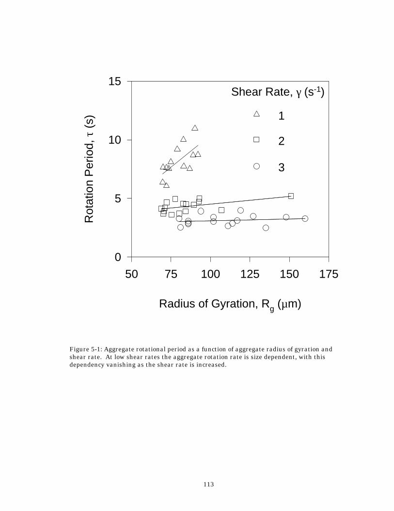
113

Figure 5-1: Aggregate rotational period as a function of aggregate radius of gyration and shear rate. At low shear rates the aggregate rotation rate is size dependent, with this dependency vanishing as the shear rate is increased.

Radius of Gyration, Rg (µm)

50 75 100 125 150 175

Rot

atio

n P

erio

d, τ

(s)

0

5

10

15Shear Rate, γ (s-1)

2

3

1

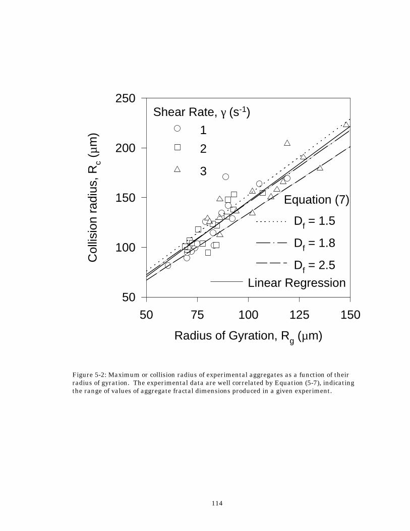
114

Figure 5-2: Maximum or collision radius of experimental aggregates as a function of their radius of gyration. The experimental data are well correlated by Equation (5-7), indicating the range of values of aggregate fractal dimensions produced in a given experiment.


50 75 100 125 150

Col

lisio

n ra

dius

, Rc

(µm

)

50

100

150

200

250Shear Rate, γ (s-1)

1

2

3

Linear Regression

Equation (7)

Df = 1.8

Df = 2.5

Df = 1.5

115

Figure 5-3: Comparison of cross-sectional aggregate areas measured by image analysis with values calculated using the aggregate collision radius and radius of gyration. The aggregate outer radius over estimates the aggregate cross-sectional area significantly.


50 75 100 125 150

Are

a (µ

m2 ) Image Analysis

πRc2

Area Basis

0

πRg2

2 x 105

1 x 105

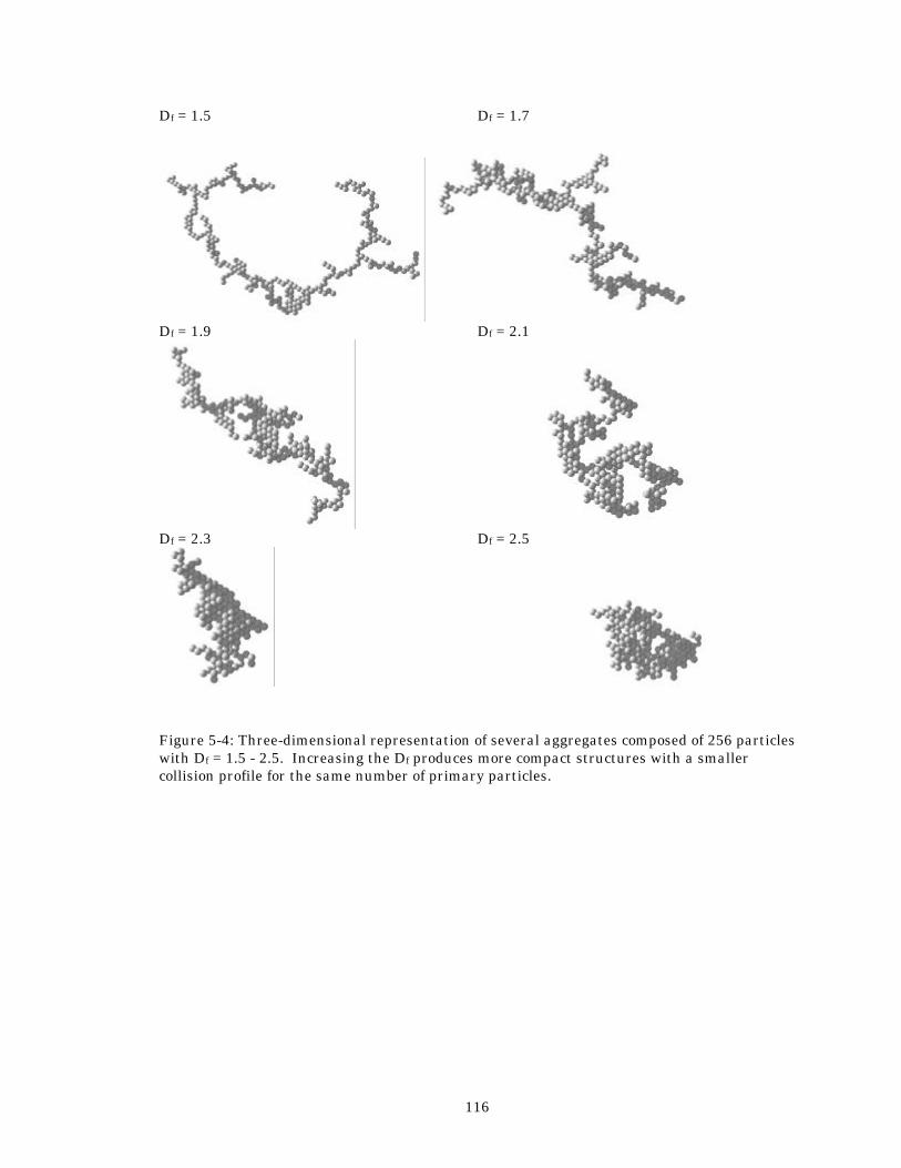
116

Df = 1.5 Df = 1.7

Df = 1.9 Df = 2.1

Df = 2.3 Df = 2.5

Figure 5-4: Three-dimensional representation of several aggregates composed of 256 particles with Df = 1.5 - 2.5. Increasing the Df produces more compact structures with a smaller collision profile for the same number of primary particles.

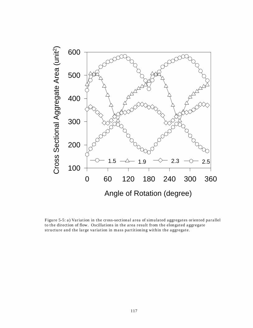
117

Figure 5-5: a) Variation in the cross-sectional area of simulated aggregates oriented parallel to the direction of flow. Oscillations in the area result from the elongated aggregate structure and the large variation in mass partitioning within the aggregate.

Angle of Rotation (degree)

0 60 120 180 240 300 360

Cro

ss S

ectio

nal A

ggre

gate

Are

a (u

nit2 )

100

200

300

400

500

600

1.5 1.9 2.3 2.5

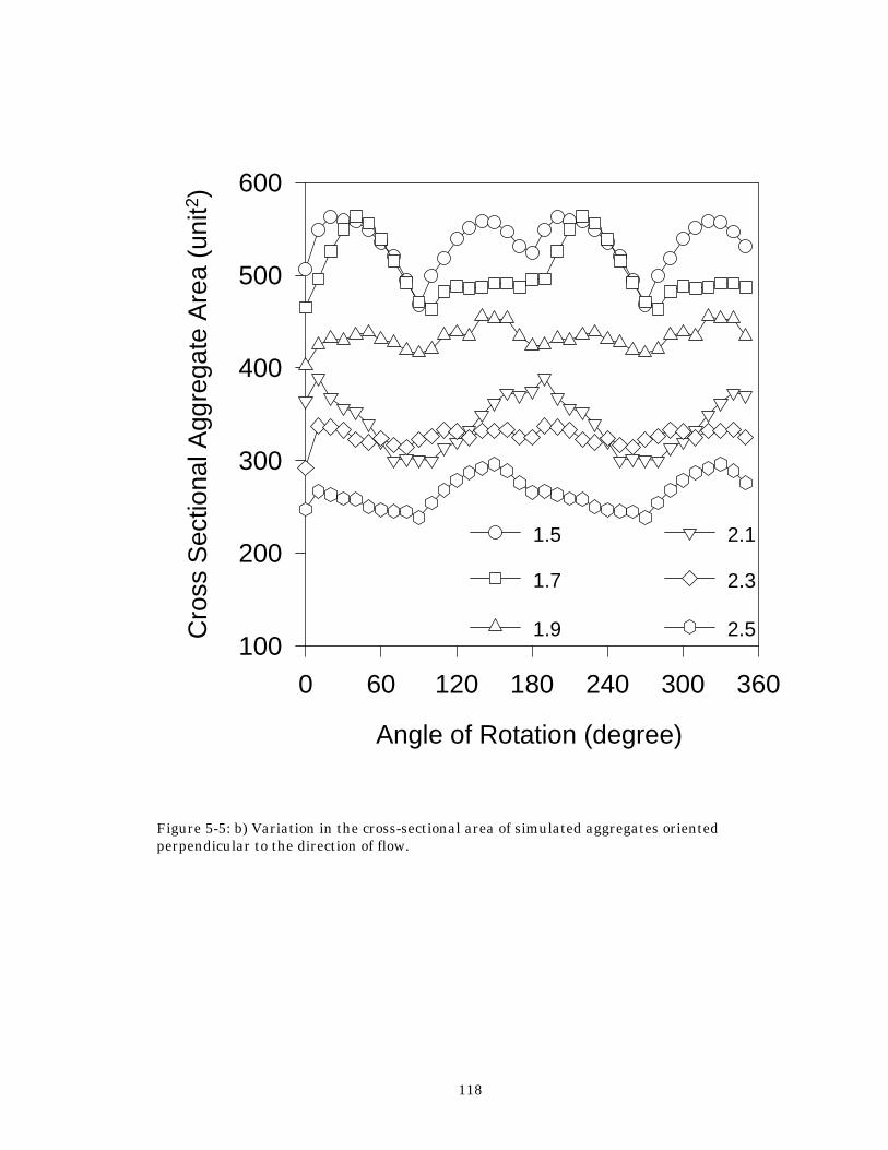
118

Figure 5-5: b) Variation in the cross-sectional area of simulated aggregates oriented perpendicular to the direction of flow.

Angle of Rotation (degree)

0 60 120 180 240 300 360

Cro

ss S

ectio

nal A

ggre

gate

Are

a (u

nit2 )

100

200

300

400

500

600

1.5

1.7

1.9

2.1

2.3

2.5

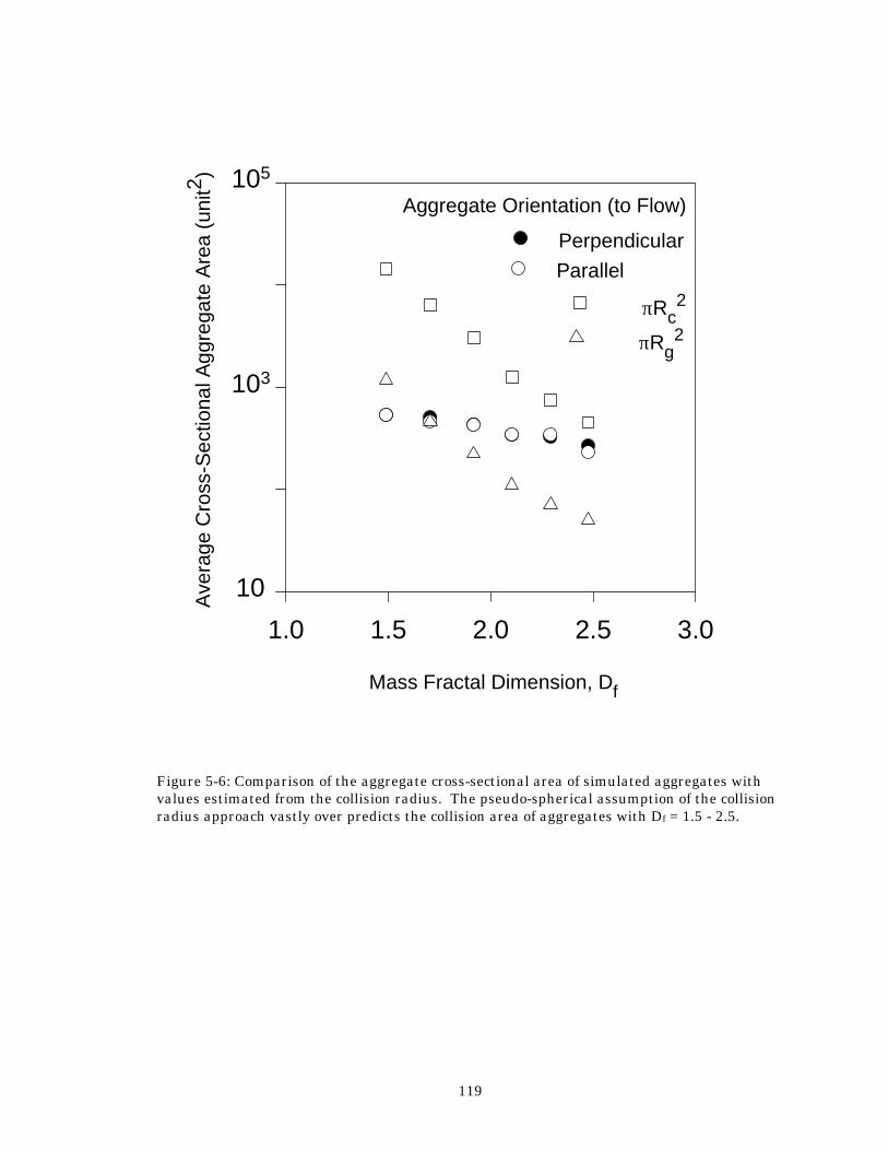
119

Figure 5-6: Comparison of the aggregate cross-sectional area of simulated aggregates with values estimated from the collision radius. The pseudo-spherical assumption of the collision radius approach vastly over predicts the collision area of aggregates with Df = 1.5 - 2.5.

Mass Fractal Dimension, Df

1.0 1.5 2.0 2.5 3.0

Ave

rage

Cro

ss-S

ectio

nal A

ggre

gate

Are

a (u

nit2 )

Aggregate Orientation (to Flow)

πRc2

πRg2

PerpendicularParallel

10

103

105

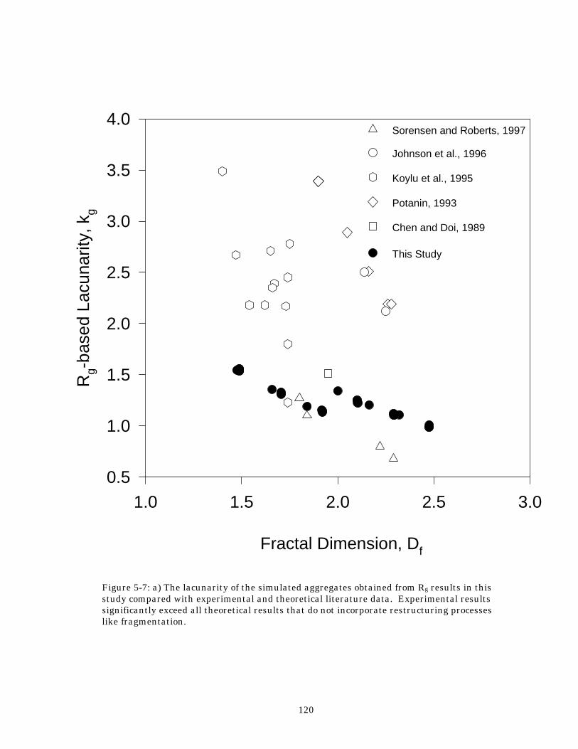
120

Figure 5-7: a) The lacunarity of the simulated aggregates obtained from Rg results in this study compared with experimental and theoretical literature data. Experimental results significantly exceed all theoretical results that do not incorporate restructuring processes like fragmentation.

Fractal Dimension, Df

1.0 1.5 2.0 2.5 3.0

Rg-

base

d La

cuna

rity,

kg

0.5

1.0

1.5

2.0

2.5

3.0

3.5

4.0Sorensen and Roberts, 1997

Johnson et al., 1996

Koylu et al., 1995

This Study

Chen and Doi, 1989

Potanin, 1993

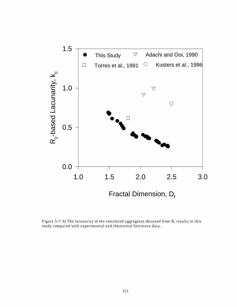
121

Figure 5-7: b) The lacunarity of the simulated aggregates obtained from Rc results in this study compared with experimental and theoretical literature data.

Fractal Dimension, Df

1.0 1.5 2.0 2.5 3.0

Rc-

base

d La

cuna

rity,

kc

0.0

0.5

1.0

1.5This Study

Kusters et al., 1996Torres et al., 1991

Adachi and Ooi, 1990

122

Chapter 6 - Laminar and Turbulent Shear-Induced Flocculation of Fractal Aggregates An accurate description of coagulation and fragmentation of fractal-like polystyrene-Al(OH)3 aggregates in a stirred tank is developed and evaluated. The flocculation kinetics of fractal aggregates are evaluated experimentally and theoretically by laser light scattering and population balance modeling. The average aggregate size increases before reaching a constant steady state value during flocculation in a stirred tank. Increasing the applied shear rate increases the rate of flocculation, decreasing the time lag before steady state and the steady state average aggregate size. A constant aggregate structure independent of shear rate was determined by assuming a fractal-like morphology, giving a mass fractal dimension Df = 2.1. A population balance model describing simultaneous aggregate coagulation and fragmentation and the effects of aggregate structure and hydrodynamic interactions was found to model the stirred tank data and literature data from a laminar shear system quite well. This chapter has been published: Flesch, J. C., Spicer, P. T. and Pratsinis, S. E., "Laminar and Turbulent Shear-Induced Flocculation of Fractal Aggregates," AIChE J., 45, 1114-1124 (1999).

123

Introduction Irregular, fractal aggregates form during shear-induced collisions as particles adhere to one another in their instantaneous random orientations, increasing the average particle size (Mandelbrot, 1983; Meakin, 1988). These aggregates have a much larger collision profile than their volume equivalent spherical counterparts, which enhances collision rates (Tambo and Watanabe, 1979; Jiang and Logan, 1991; Wiesner, 1992) and reduces the fluid viscous resistance to collisions (Kusters et al., 1996). Hierarchical simulations of aggregate-aggregate collisions predict a fractal dimension, Df = 1.8 while particle-cluster collisions produce a more compact Df ≅ 3 (Torres et al., 1991), though particle-cluster collisions will only alter realistic aggregate structures to a small extent (Df = 2) (Kusters et al., 1996). Aggregates are fragmented by fluid shear stresses more rapidly than compact mass equivalent particles at a rate dependent on the applied shear rate, the aggregate structure, and the bonds between primary particles (Sonntag and Russell, 1986, 1987; Horwatt et al., 1992; Potanin, 1993). Aggregate restructuring to a more compact form may also occur by reformation of fragments (Clark and Flora, 1991) or by shear interactions that rearrange the aggregate structure (Oles, 1992). After a characteristic time, a steady state is reached between coagulation and fragmentation characterized by an aggregate size distribution that does not change with time and is a unique for a given system (Spicer and Pratsinis, 1996a). The shear environment of a stirred tank flocculator is complex, position-dependent, and especially intense in the region surrounding the impeller. Flocculation models must incorporate the dependency of flocculation kinetics on floc structure, the fluid shear field, and their mutual interactions. Previous studies of fractal aggregate dynamics in stirred tanks modeled only short residence times and ignored fragmentation (Wiesner, 1992). The objective of this work is to study the effect of aggregate structure on simultaneous shear-induced coagulation and fragmentation using kinetic expressions incorporating the aggregate structure. Existing work on the reduction of aggregate viscous effects and the flow of particles in a stirred tank are used to accurately model flocculation dynamics. Comparisons are made with experimental data for the evolution of aggregate size and structure in a stirred tank and conclusions are drawn as to the accuracy of assuming a constant fractal dimension for a flocculating particle suspension.

Theory

Particle Size Distribution The dynamic behavior of the particle size distribution undergoing simultaneous coagulation and fragmentation is given by (Friedlander, 1977; Vigil and Ziff, 1989):

dndt

=12

(u ,u )n n - n (u ,u )n - S n + S ni

j+k=ij k j k i

k=1k i k i i

j=i

imax

j j∑ ∑ ∑∞

αβ αβ γ i j, (6-1)

where ni is the number concentration of flocs of size i (meaning that a single floc contains i primary particles). The first term on the right hand side (RHS) of Equation (2-1) represents the formation of particles comprised of i primary particles by collisions of smaller j- and k-sized particles. The second RHS term denotes the loss of particles of size i by collision with particles of any other size. The third RHS term describes the loss of particles of size i by fragmentation and the fourth RHS term describes the formation of particles of size i by the fragmentation of larger particles.

124

A numerical solution of Equation (2-1) is obtained based on Hounslow et al. (1988) in terms of sections (size classes) of the particle size distribution (Spicer and Pratsinis, 1996a):

i

j=1

i -2j -i+1

i -1, j i 1 j i -1,i -1 i -12

ij=1

i -1j -i

i, j j

ij=i

i, j j i i i, j j j

imax

dNdt

= 2 N N +12

N - N 2 N

- N N - S N + S N

∑ ∑

∑ ∑

−

=

αβ αβ αβ

αβi

j i

max

Γ

(6-2)

where Ni is the number concentration of flocs of size class i (meaning that a single floc contains 1.5*2i-1 primary particles), α is the collision efficiency for coagulation and βi,k is the collision frequency for particles of size class i and k with characteristic volumes vi and vk, Si is the fragmentation rate of flocs of volume vi, and Γi,j is the breakage distribution function defining the volume fraction of the fragments of size i coming from j-sized particles.

Aggregates The rate expressions describing aggregate coagulation and fragmentation are size

dependent. As a result, the increased characteristic size of irregular aggregates versus mass equivalent spheres must be incorporated into a model of aggregate dynamics. The structure of aggregates can be quantified using their mass fractal dimension, Df, a measure of the floc compactness that varies from 1, for an aggregate made of a line of particles, to 3, for a compact aggregate of primary particles. The mass of a fractal floc (M) varies with its characteristic length (l) as (Mandelbrot, 1987):

M lD f∝ (6-3)

and maximum or collision radius, Rci, of an aggregate with size i and primary particles of radius a, is given by (Kusters et al., 1996):

i kRac

ciDf

=

(6-4)

where kc is the aggregate lacunarity (here assumed to be = 1). However, it should be noted that recent work indicates this assumption my under estimate kc (Neimark et al., 1996; Spicer, 1997). The aggregate collision radius can be significantly larger than its mass equivalent spherical radius as Df decreases below 3.

Coagulation In laminar shear flow, the binary collision rate between particles of size i and j as a result of the average velocity gradient, γ, is (Smoluchowski, 1917):

( )3jij,i aa34

+γ=β (6-5)

where ai is the radius of a particle of size i. The coagulation rate of neutrally buoyant spherical particles smaller than the Kolmogorov microscale, η, in homogeneous, isotropic turbulence is given by (Saffman and Turner, 1956):


+1294

1

2 3 (6-6)

125

where ε is the characteristic turbulent energy dissipation rate of the stirred tank, and ν is the kinematic viscosity of the suspending fluid.

Equation (2-3) is modified to account for the effect of floc structure on collision frequencies by substituting the collision radius (Equation (6-4)) for the volume equivalent radius (Jiang and Logan, 1991):

βενi j c

D D Da k i jf f f, .=

+

−

1294 3

31

21 1 3

(6-7)

where i is the number of primary particles comprising an i-sized floc, and Df is the mass fractal dimension of an aggregate. Equation (6-7) assumes that the collision sphere surrounding the aggregate represents its collision profile. This approach is thus a maximum estimate of the enhancement of collision frequencies by aggregate structure.

Viscous Retardation of Collisions As two spherical particles approach one another in fluid shear, the viscous fluid layer between them resists collision, in some cases completely (Adler, 1981). Porous aggregate structures permit internal fluid flow, decreasing the viscous resistance. Kusters et al. (1996) developed a model of aggregate collision efficiency by representing aggregates as dense cores surrounded by porous shells and calculated the permeability to fluid based on a fractal model of aggregate structure. The detailed model of Kusters et al. (1996) has been implemented here in order to account for the reduction in collision frequency by viscous effects.

Fragmentation The rate of fragmentation by splitting of a particle of radius ai is given by (Delichatsios and Probstein, 1976; Kusters, 1991):

Su

au

uii

b=

−

21

2 2

2π∆ ∆

∆exp (6-8)

where ∆u is the rms velocity difference across the distance ai and ∆ub is the critical velocity difference at which breakage of the floc occurs. Substituting into Equation (6-8) for ∆u and ∆ub gives the simplified form of the breakage rate (Kusters, 1991):

Sib=

−

415

12

12

πεν

εε

exp (6-9)

where εb is the critical turbulent energy dissipation rate at which flocs fragment. Because aggregate fragmentation is rather poorly understood, the εb must be related

to floc size in a way consistent with the fact that εb decreases with increasing floc size since larger particles are more susceptible to turbulent shear stresses. A power-law relationship between floc size and shear rate is commonly used to correlate experimental (Tambo and Watanabe, 1979) and simulation results (Potanin, 1993):

R Gim∝ − (6-10)

where m varies between 0.4 and 5 for turbulent flow and various floc types (Table 1). The theory of aggregate fragmentation is not as definitive as that for shear-induced coagulation.

126

As a result, it is sufficiently accurate to choose an expression that is physically consistent with experimental data:

ε biHi

BR

= (6-11)

where A is an additional fitting parameter. Equation (6-11) predicts an inverse relationship between energy dissipation rate and aggregate size, as flocs grow larger they are more susceptible to fragmentation by fluid shear. The effect of floc structure is also included by using the hydrodynamic radius, RHi as a measure of floc size that increases with decreasing Df (Kusters et al., 1996), thus accounting for the larger profile of fractal aggregates over spherical equivalent particles. The flocs are assumed to split upon fragmentation (binary fragmentation). A broader fragment size distribution (i.e. ternary or normal distribution) has little effect on the evolution of integral properties but tends to broaden the steady state particle size distribution versus binary fragmentation (Spicer and Pratsinis, 1996a).

Experimental Flocculation of an aqueous suspension of monodisperse, spherical, polystyrene particles (d0 = 0.87 µm) was studied in a 2.8 liter, baffled, stirred tank of standard configuration (Spicer and Pratsinis, 1996b). The suspension was mixed using a radial flow (Rushton) Lightnin R100 impeller. The center of the impeller was positioned at 1/3 the

height of the tank. The solids volume fraction was φ =1.4 x 10-5, corresponding to an initial particle number concentration of 4 x 107 cm-3. The flocculant was aluminum sulfate hydrate (Al2(SO4)3 16H2O; Aldrich, 98%) (Clark and Flora, 1991). All experiments were conducted using a constant Al2(SO4)3 16H2O concentration of 10 mg/liter. Sodium hydrogen carbonate (NaHCO3; Aldrich, 99%) at a concentration of 1mM was used to buffer the suspension and the pH was kept at 7.2 ± 0.05 during all experiments.

The polystyrene suspension was first mixed at G = 300 s-1 for five minutes to break up any agglomerates. The flocculant was then added and mixed with the suspension for one minute. The impeller was then set to the desired speed. The impeller rotational velocity was measured using an optical tachometer (Onno Sokki HT-4100) and varied by less than 1 RPM. All experiments were carried out 2-3 times and very little variation was observed. The turbulent shear rate within the stirred tank was approximately characterized using the spatially averaged velocity gradient, G, following the procedures of Spicer and Pratsinis (1996b).

The floc sampling technique is crucial to accurately characterize flocculation dynamics. A large number of particles (>500) must be sampled to accurately determine a floc size distribution while care must be taken not to alter fragile floc structures by sampling / removal procedures. Samples were obtained for analysis by one of two techniques: 1. Withdrawal of a sample to be placed into the sample cell using a 5 mm i. d. pipette (Clark and Flora, 1991). This technique was used only when very low shear rates were used for flocculation (G = 15, 25 s-1). 2. Gentle withdrawal of a sample into the flow-through sample cell using a syringe (Ng et al., 1993) was used for suspensions flocculated at G = 50, 100, and 150 s-1. Samples were withdrawn from the same location in the tank, midway between the impeller and the top of the suspension (bulk zone).

Small angle light scattering measurements by a Malvern Mastersizer E (Malvern Instruments) were used to evaluate the floc size distribution and the average floc structure and density as a function of time. The structure of the flocs was determined quantitatively by their mass fractal dimension, Df, a measure of the floc compactness that varies from 1, for a floc made of a line of particles, to 3, for a compact spherically-shaped floc of primary

127

particles (Mandelbrot, 1987). The mass of a fractal floc varies with its characteristic length (l) as:

M lD f∝ (6-12)

The scattering behavior of suspended particles is dependent on the ratio of primary particle size, d0, to the wavelength of light scattered, λ, so that if

d0 >> λ (6-13)

the fractal dimension, Df, is determined from the slope (m = Df -3) of a log-log plot of the ratio of the initial suspended particle volume fraction φp to that of the flocculated suspension, φf, versus the mass mean diameter, dmm, of the floc size distribution based on rearrangement of Equation (6-12) (Oles, 1992; Kusters et al., 1996):

φ

φp

fmm

Dd f∝ −3 (6-14)

The apparent volume fraction of the suspended flocs is a function of the obscuration, OB, of the laser beam, a parameter reported by the Mastersizer E (Kusters, 1991; Kusters et al., 1996):

φ fsmd OB

L=

−ln( )13

(6-15)

with dsm, the Sauter mean diameter of the size distribution (Kusters et al., 1996), and L, the laser path length (2.1 mm). This technique of floc structural characterization allows measurement of the average floc fractal dimension over the duration of the experiment. Characterization of floc restructuring is also possible when multiple slopes are present (Oles, 1992).


Effect of Aggregate Structure on Flocculation Kinetics The larger collision area of aggregates relative to spheres enhances their collision frequency (Equation (6-4)). As a result, decreasing the aggregate fractal dimension, Df, will have a significant effect on flocculation kinetics. Figure 6-1 shows the calculated evolution of the dimensionless mass mean aggregate diameter with time by coagulation for various Df. At all Df, the aggregate size increases exponentially with time, consistent with Vigil and Ziff (1989). A large enhancement of the aggregate growth rate is seen in Figure 6-1 as Df is decreased from 3 to 2 and the average aggregate size is increased by as much as a factor of 5 at a given time. Analysis of the evolution of the average aggregate density, φf, with time indicates that the aggregates produced in this study possess a fractal dimension Df = 2.1 independent of shear rate, in excellent agreement with the early stages of laminar shear-induced aggregation (Oles, 1992). Porous, fractal aggregates will be more susceptible to fragmentation by fluid shear stresses than equivalent spherical particles (Sonntag and Russell, 1986). As a result, the theoretical description of fragmentation rates must account for this dependency. Figure 6-2 shows the calculated aggregate fragmentation rates as a function of aggregate mass and structure for B = 4.7 and Df = 2.1, 2.5, and 3. Equations (6-9) and (6-11) predict an exponential increase in fragmentation rates with aggregate size, consistent with experimental evidence for a sharply increased influence of shear stresses at a certain

128

threshold aggregate size (Pandya and Spielman, 1982; Spicer and Pratsinis, 1996b). A transition from Df = 3 to Df = 2.5 to Df = 2.1 increases the characteristic aggregate size for a constant number of primary particles, increasing the likelihood that shear-induced fragmentation will occur. The fragmentation rate of increasingly open aggregate structures is thus significantly higher than for more compact aggregates.

Comparison with Experimental Data In order to model the shear-induced aggregation of polystyrene spheres by alum it is necessary to characterize the initial conditions accurately. Although the suspensions is initially monodisperse, the mixing of flocculant requires the application of high fluid shear rates. Inevitably some flocculation will occur in this time, and the fractal nature of the aggregates produced will considerably alter the initial size distribution. For this reason the aggregate size distribution measured following the rapid mix period (Error! Reference source not found.) was used as the initial condition in all simulations of stirred tank data. Figure 6-4 shows the evolution of the mass mean aggregate collision diameter, dmm, with time for a range of values of the spatially averaged velocity gradient, G (50, 100, 150 s-1). For all three shear rates examined, an initial increase in dmm is observed as coagulation increases the average particle size, in agreement with Figure 6-1. For all three shear rates (G = 50, 100, 150 s-1) fragmentation becomes significant after some time and the aggregation rate slows until a steady state is reached between coagulation and fragmentation and the average size no longer changes. This is consistent with experimental observations of turbulent (Spicer and Pratsinis, 1996b) and laminar (Oles, 1992) shear-induced flocculation. For all shear rates, increasing the G increases the coagulation rate and the rate at which dmm increases with time as particles collide more rapidly. In addition, fragmentation is more significant with increasing shear rate, opposing coagulation more rapidly and decreasing the time lag before attainment of steady state (Spicer and Pratsinis, 1996a).

The solid lines in Figure 6-4 are the predictions of the theoretical model and are in excellent agreement with the experimental data at the three highest shear rates (G = 50, 100, 150 s-1). In all simulations Df = 2.1 and the collision efficiency, α, was obtained from Kusters et al. (1996). It should be emphasized here that only one fitting parameter was used in the model. The parameter B in Equation (6-9) was chosen such that agreement is obtained between theory and data for the steady state average aggregate size observed experimentally. One factor not accounted for by this analysis is the heterogeneity of the fluid flow field in the stirred tank, which may cause the average shear rate to deviate from the spatially averaged value calculated from the power input. The good agreement in Figure 6-4, however, indicates that G characterizes the stirred tank system quite well at these shear rates.

Comparison with Literature Data The data of Oles (1992) for the aggregation of 2.17 µm polystyrene particles with NaCl in laminar shear are shown in Figure 6-5 as a function of shear rate. An identical trend is observed for laminar shear-induced aggregation as for turbulent shear (Figure 6-4) an initial increase in size followed by attainment of a steady state value. Spicer and Pratsinis (1996a) modeled these data using a simplified form of the present model with a collision efficiency α = 1 that ignored aggregate structure and viscous interactions. They acknowledged that this value was artificial but necessary to account for the effects of aggregate structure on flocculation kinetics. Oles (1992) measured an average aggregate fractal dimension of Df = 2.3, and the current model is able to describe these data quite well using this parameter as input while accounting for viscous interactions and again fitting the fragmentation dominated range of data by merely adjusting the value of B.

129

Conclusions A population balance model of the coagulation and fragmentation of fractal aggregates was developed that accounts for aggregate structure and its effect on particle-particle and particle-fluid interactions. The model predictions were in excellent agreement with the time evolution of the mass average aggregate size produced in laminar and turbulent shear.

Acknowledgments Financial support by Genencor International B. V. is gratefully acknowledged.

130

Notation aI radius of particle with index i (µm) B breakage rate coefficient (cm-3a s-1) d0 primary particle diameter (µm) dmm mass mean particle diameter (µm) dsm Sauter mean particle diameter (µm) Df fractal dimension (-) G spatially averaged shear rate (s-1) i number of particles in an aggregate (-) kc lacunarity (-) l characteristic length (µm) L laser beam path length (cm) m breakage rate exponent (-) M mass (g) N0 initial number concentration (# / cm3) ni discrete number concentration of particles with index i (# / cm3) Ni sectional number concentration of particles with index i (# / cm3) OB laser beam obscuration (-) Q laser wavenumber (-) Rc aggregate collision radius (µm) RH aggregate hydrodynamic radius (µm) Si particle fragmentation rate (s-1) u fluid velocity (cm/s)

ub critical breakage velocity (cm/s)

Greek Letters α collision efficiency (-) β i,j collision frequency (cm3/s) γ laminar shear rate (s-1) γ i,j discrete fragment size distribution of size i fragments (-) Γ i,j sectional fragment size distribution of size i fragments (-) ε energy dissipation rate (cm2/s3) εb critical fragmentation energy dissipation rate (cm2/s3) φf flocculated dispersion density (-) φp solids volume fraction (-) η Kolmogorov microscale (µm) λ laser wavelength (nm) ν kinematic viscosity (cm2 / s)

131

References Adler, P. M., “Heterocoagulation in Shear Flow,” J. Colloid Interface Sci., 83, 106-115 (1981). Clark, M. M., and Flora, J. R. V., "Floc Restructuring in Varied Turbulent Mixing," J. Colloid

and Interface Sci., 147, 407-421 (1991). Delichatsios, M. A., and Probstein, R. F., "The Effect of Coalescence on the Average Drop Size

in Liquid-Liquid Dispersions," Ind. Eng. Chem., Fund., 15, 134-138 (1976). Francois, R. J., "Strength of Aluminum Hydroxide Flocs," Water Research, 21, 1025-1030

(1987). Friedlander, S. K., Smoke, Dust, and Haze, Wiley, New York, (1977). Horwatt, S. W., Feke, D. L., amd Manas-Zloczower, I., “The Influence of Structural

Heterogeneities on the Cohesivity and Breakup of Agglomerates in Simple Shear Flow,” Powder Tech., 72, 113-119 (1992).

Hounslow, M. J., Ryall, R. L., and Marshall, V. R., "A Discretized Population Balance for Nucleation, Growth, and Aggregation," AIChE J., 34, 1821-1832 (1988).

Jiang and Logan, B. E., “Fractal Dimensions of Aggregates Determined from Steady State Size Distributions,” Env. Sci. and Tech., 25, 2031-2038 (1991).

Jullien, R. and Botet, R., Aggregation and Fractal Aggregates, World Scientific, Singapore, (1987).

Kusters, K. A., "The Influence of Turbulence on Aggregation of Small Particles in Agitated Vessels," Ph. D. Dissertation, Eindhoven University of Technology, The Netherlands, (1991).


Leentvaar, J. and Rebhun, M., "Strength of Ferric Hydroxide Flocs," Water Res., 17, 895-902 (1983).


Meakin, P., "Fractal Aggregates," Adv. Colloid Interface Sci., 28, 249-331 (1988). Neimark, A. V., Koylu, U. O., and Rosner, D. E., “Extended Characterization of Combustion-

Generated Aggregates: Self-Affinity and Lacunarities,” J. Colloid Interface Sci., 180, 590 (1996).

Ng, K. W. K., Amal, R., Raper, J. A., and Waite, T. D., “The Effects of Alum Concentration and pH on the Aggregation Kinetics of Colloidal Haematite,” Proceedings of the Sixth International Symposium on Agglomeration, 785, Nagoya, Japan, (1993).


Pandya, J. D. and Spielman, L. A., "Floc Breakage in Agitated Suspensions: Theory and Data Processing Strategy," J. Colloid Interface Sci., 90, 517-531 (1982).



Smoluchowski, M., “Versuch Einer Mathematischen Theorie de Koagulations- Kinetic Kolloider Losungen,” Z. Phys. Chem., 92, 129-168 (1917).



Spicer, P. T. and Pratsinis, S. E., “Coagulation-Fragmentation: Universal Steady State Particle Size Distributions,” AIChE J., 42, 1612-1620 (1996a).

Spicer, P. T. and Pratsinis, S. E., “Shear-Induced Flocculation: The Evolution of Floc Structure and the Shape of the Size Distribution at Steady State,” Wat. Res., 30, 1049-1056 (1996b).

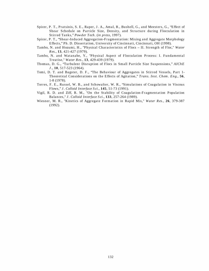
132

Spicer, P. T., Pratsinis, S. E., Raper, J. A., Amal, R., Bushell, G., and Meesters, G., “Effect of Shear Schedule on Particle Size, Density, and Structure during Flocculation in Stirred Tanks,” Powder Tech. (in press, 1997).

Spicer, P. T., “Shear-Induced Aggregation-Fragmentation: Mixing and Aggregate Morphology Effects,” Ph. D. Dissertation, University of Cincinnati, Cincinnati, OH (1998).

Tambo, N. and Hozumi, H., "Physical Characteristics of Flocs – II. Strength of Floc," Water Res., 13, 421-427 (1979).



Tomi, D. T. and Bagster, D. F., “The Behaviour of Aggregates in Stirred Vessels, Part 1-Theoretical Considerations on the Effects of Agitation,” Trans. Inst. Chem. Eng., 56, 1-8 (1978).


Vigil, R. D. and Ziff, R. M., "On the Stability of Coagulation-Fragmentation Population Balances," J. Colloid Interface Sci., 133, 257-264 (1989).

Wiesner, M. R., "Kinetics of Aggregate Formation in Rapid Mix," Water Res., 26, 379-387 (1992).

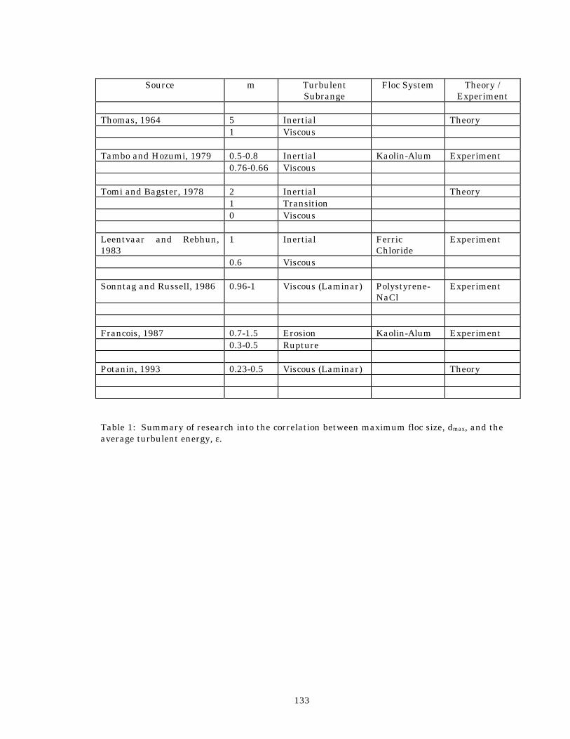
133

Source m Turbulent

Subrange Floc System Theory /

Experiment Thomas, 1964 5 Inertial Theory 1 Viscous Tambo and Hozumi, 1979 0.5-0.8 Inertial Kaolin-Alum Experiment 0.76-0.66 Viscous Tomi and Bagster, 1978 2 Inertial Theory 1 Transition 0 Viscous Leentvaar and Rebhun, 1983

1 Inertial Ferric Chloride

Experiment

0.6 Viscous Sonntag and Russell, 1986 0.96-1 Viscous (Laminar) Polystyrene-

NaCl Experiment

Francois, 1987 0.7-1.5 Erosion Kaolin-Alum Experiment 0.3-0.5 Rupture Potanin, 1993 0.23-0.5 Viscous (Laminar) Theory Table 1: Summary of research into the correlation between maximum floc size, dmax, and the average turbulent energy, ε.

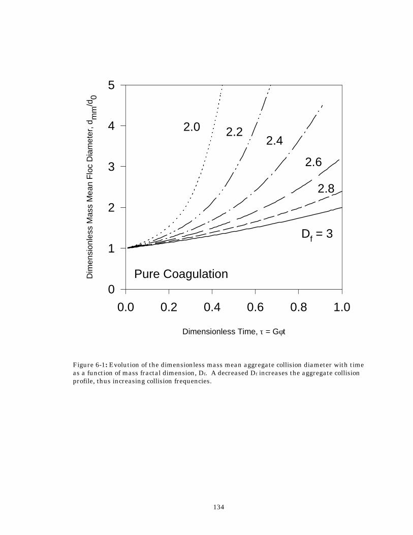
134

Figure 6-1: Evolution of the dimensionless mass mean aggregate collision diameter with time as a function of mass fractal dimension, Df. A decreased Df increases the aggregate collision profile, thus increasing collision frequencies.


0.0 0.2 0.4 0.6 0.8 1.0

Dim

ensi

onle

ss M

ass

Mea

n F

loc

Dia

met

er, d

mm

/d0

0

1

2

3

4

5

Df = 3

2.8

2.6

2.42.22.0

Pure Coagulation

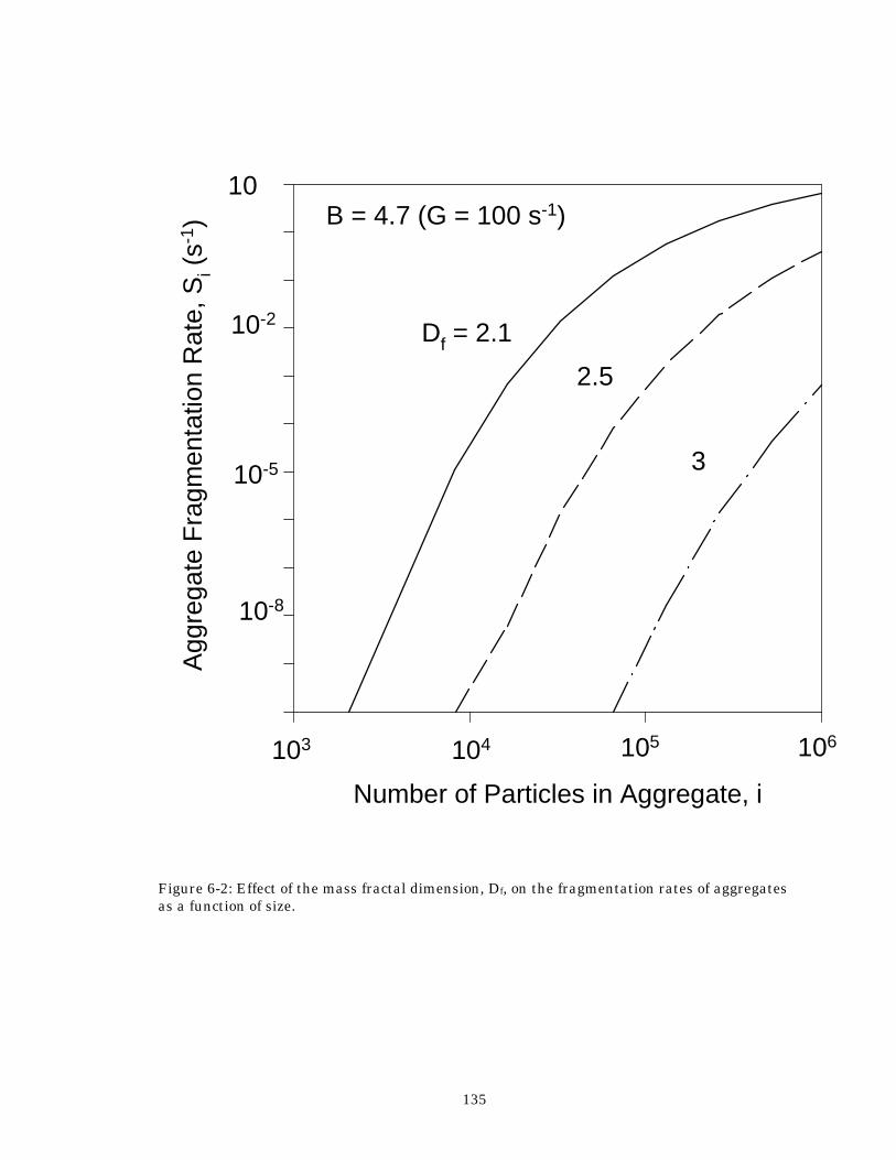
135

Figure 6-2: Effect of the mass fractal dimension, Df, on the fragmentation rates of aggregates as a function of size.

Number of Particles in Aggregate, i

Agg

rega

te F

ragm

enta

tion

Rat

e, S

i (s-1

)

Df = 2.1

2.5

3

B = 4.7 (G = 100 s-1)10

10-2

10-5

10-8

106103 104 105

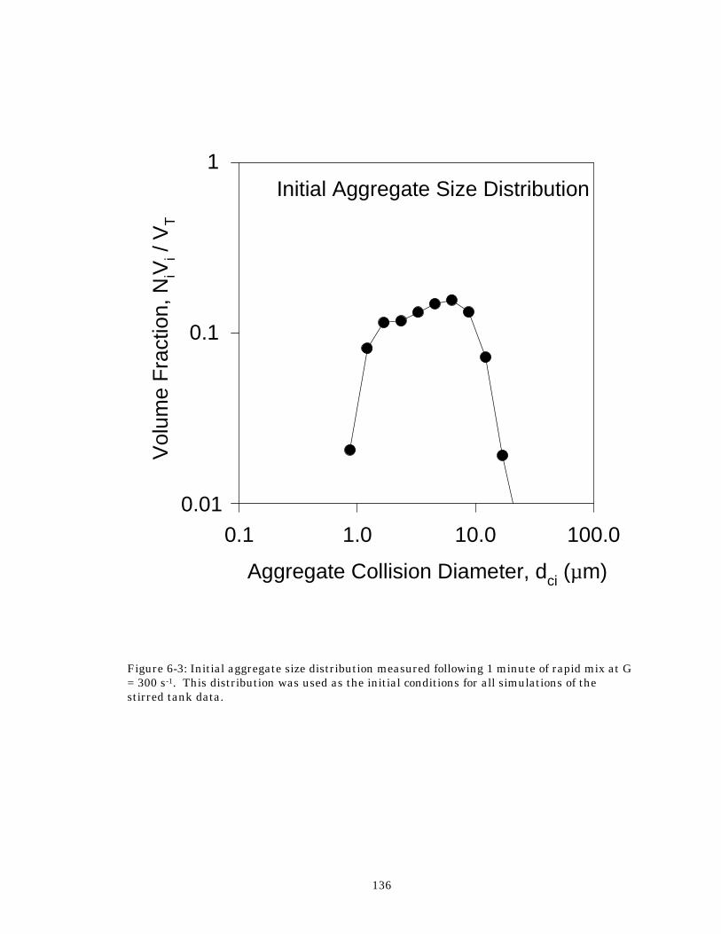
136

Figure 6-3: Initial aggregate size distribution measured following 1 minute of rapid mix at G = 300 s-1. This distribution was used as the initial conditions for all simulations of the stirred tank data.

Aggregate Collision Diameter, dci (µm)

0.1 1.0 10.0 100.0

Vol

ume

Fra

ctio

n, N

iVi /

VT

0.1

1Initial Aggregate Size Distribution

0.01

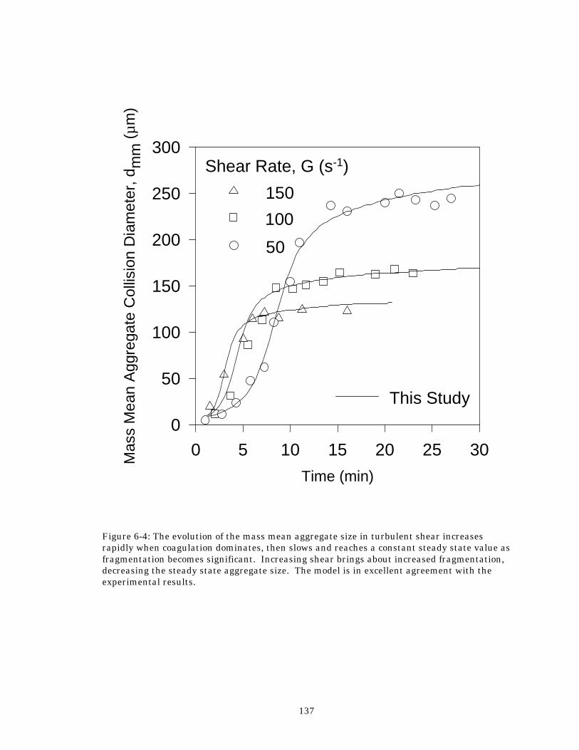
137

Figure 6-4: The evolution of the mass mean aggregate size in turbulent shear increases rapidly when coagulation dominates, then slows and reaches a constant steady state value as fragmentation becomes significant. Increasing shear brings about increased fragmentation, decreasing the steady state aggregate size. The model is in excellent agreement with the experimental results.

Time (min)

0 5 10 15 20 25 30Mas

s M

ean

Agg

rega

te C

ollis

ion

Dia

met

er, d

mm

(µm

)

0

50

100

150

200

250

300Shear Rate, G (s-1)

This Study

50

100

150

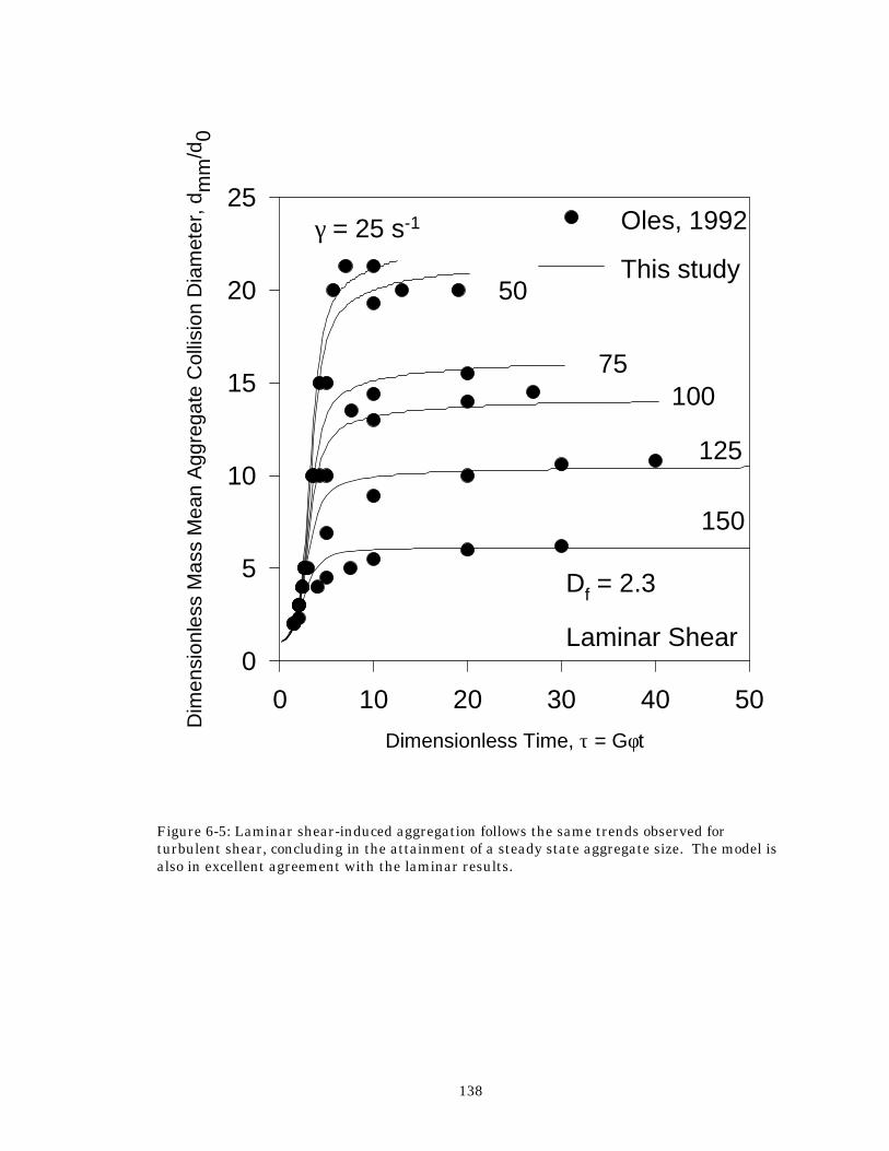
138

Figure 6-5: Laminar shear-induced aggregation follows the same trends observed for turbulent shear, concluding in the attainment of a steady state aggregate size. The model is also in excellent agreement with the laminar results.


0 10 20 30 40 50

Dim

ensi

onle

ss M

ass

Mea

n A

ggre

gate

Col

lisio

n D

iam

eter

, dm

m/d

0

0

5

10

15

20

25γ = 25 s-1

50

75100

125

150

Oles, 1992

This study

Df = 2.3

Laminar Shear

139

Chapter 7 - Concentrated Suspension Dynamics : Enhanced Backward Light Scattering The shear-induced flocculation of kaolin-polymer flocs in a stirred tank is investigated at medium-high solids fractions (φ = 1 - 10% w/w). The average floc size evolution is monitored by changes in intensity of laser light scattered in the 180° direction. The measurements reflect the change in particle number concentration as flocculation proceeds. As flocculation begins, coagulation dominates and the floc size increases (total particle number decreases) and then levels off at a steady state value as fragmentation becomes significant and balances coagulation. At steady state, the measurements indicate the extent of flocculation. Increasing the shear rate increases the coagulation and fragmentation rates, resulting in smaller floc sizes at steady state. Increasing the flocculant concentration increases the steady state floc size by strengthening the bonds between primary particles to resist fragmentation. At constant shear rate and flocculant concentration, increasing the solids fraction decreases the steady state floc size indicating formation of weakly bonded flocs. This chapter has been published: Spicer, P. T., Pratsinis, S. E., Willemse, A. W., Merkus, H. G. and Scarlett, B., "Monitoring the Dynamics of Concentrated Suspensions by Enhanced Backward Light Scattering," Part. Part. Syst. Charact., 16, 201-206 (1999).

140

Introduction Historically, the theoretical and experimental work carried out on flocculation has been extensive, but directed predominantly toward dilute suspensions of particles (i.e. volume fraction φ = 10-6 - 10-3). However, improvements in process technology as well as the growing significance of biotechnology and materials processing emphasize the need for a shift in the focus of flocculation research toward more concentrated suspensions of particles. An example is industrial cell cultures, these suspensions can reach volume fractions up to φ = 0.4 in an attempt to maximize the productivity of a process (Reuβ et al., 1979) . Flocculation is an integral part of many separation process loops, but the control and maintenance of such processes remains largely empirical. This is often the result of the lack of fundamental understanding of the physical phenomena of flocculation, especially with suspensions of high solids fractions. Concentrated suspensions are more difficult to characterize relative to more dilute ones, although characterization techniques are available. The opacity of most concentrated suspensions makes it impossible to apply standard light scattering techniques that rely on forward scattered light without dilution of the sample. Dilution, however, can bias a measurement and is best avoided. One method that allows in situ characterization of concentrated suspensions measures backward scattering, or the intensity of light scattered directly back toward its incident source. One version of this technology is used by Laser Sensor Technology (Seattle, WA) in their commercial Par Tec instrument. The Par Tec focuses a laser into a stirred suspension and rotates the focal point constantly to scan the suspension. When a particle crosses the circle traced by the beam focal point, it reflects light back toward the probe optics where such pulses are collected. The duration of the backward scattered light is then used to calculate the chord length of the particle scanned during each backward scattering pulse. Although this technique is the most direct measurement of particle size in concentrated suspensions, it is costly and can underestimate large particle sizes by scanning only a small portion of their surface as they pass and can overestimate small particle sizes because of the optimal focal point’s sensitivity to particle size (Monnier et al., 1996). Another method is to consider the entire assembly of particles and take advantage of the multiply scattered light that is ultimately directed back toward the incident light. It can be shown that the light scattered in this direction exceeds that at all other angles because of the constructive interference between the multiple scattering peaks of each particle (Wiersma and Lagendijk, 1997). This phenomenon (referred to as enhanced backward scattering) has been used to characterize concentrated suspensions by simultaneously directing incident light into the suspension and monitoring the light scattered backwards (Lilge et al., 1991). Heffels et al. (1996) interpreted enhanced backward scattering intensity patterns using a simple laser-camera-image analysis system and monitored relative changes in the solids volume fraction and the average particle size in latex and glass bead suspensions up to φ = 0.6. Although this method does not provide a direct measure of particle size distributions and must be calibrated, its simplicity and potential makes it attractive as a sensor for evaluating deviation from a set point in an industrial process. Until now, measurement of particle dynamics in concentrated suspensions has only been possible using elaborate and expensive instrumentation. Gregory and Gubai (1991) and Gubai and Gregory (1991) examined the polymer flocculation of suspensions of clay at solids fractions of 1-3% w/v using a commercial optical instrument (PDA 2000, Rank Bros. Ltd.) that measures the amount of light transmitted through the suspension. This technique is limited to solids concentrations that permit light transmittance (< 3 % w/v) and requires the suspension be pumped through narrow tubing for analysis, increasing the risk of altering the floc size distribution. Gregory and Gubai (1991) observed the attainment of a steady state between coagulation and fragmentation by the suspension after only a few minutes, compared to the several hours required for more dilute suspensions (Oles, 1992; Spicer et al., 1996a). The flocculation kinetics at large solids fractions were significantly affected by the amount of mixing applied during flocculant

141

addition but not at more dilute fractions. Increasing the solids fraction produced a substantial increase in the amount of flocculant required to bring about the same degree of separation. The optimum flocculation behavior was observed when the flocculant was added gradually over a period of time, rather than immediately. Williams et al. (1992) used a Par-Tec instrument to follow the flocculation of silica particles at 1-5% v/v with a polymer flocculant. They observed that the average floc size at steady state decreased with increasing shear rate. At constant shear rate and flocculant concentration, the average steady state floc size decreased with increasing solids concentration, probably because of the reduced influence of the flocculant. Incremental addition of the flocculant was found to produce a larger steady state floc size than for the simultaneous addition of the entire amount, in agreement with Gregory and Gubai (1991). The objective of this work is to evaluate the ability of an inexpensive, easy to construct apparatus allowing in situ monitoring of shear-induced kaolin flocculation at large weight fractions (φ = 0.01 - 0.1) in a stirred tank. The effect of shear rate, flocculant concentration, and solids concentration on kaolin-polymer flocculation dynamics are determined. The results of the flocculation experiments are compared with literature data obtained using relatively expensive and sophisticated commercial instruments as well as with dilute suspensions.

Particle Characterization by Backward Light Scattering

Multiple light scattering begins as light enters a concentrated assembly of particles and is first scattered by a single particle. At dilute solids fractions (< 10-4), the light would most likely pass out of the assembly without encountering another particle, but as the solids fraction is increased the probability of a second particle encounter increases. If this occurs, the phenomenon is termed multiple scattering. An interesting aspect of this phenomenon is the so called “enhanced” backward scattering that occurs at the 180° angle from the scattering event through constructive interference effects (Wiersma and Lagendijk, 1997). The result is a large scattering peak at 180° from the targeted particles that varies with particle and suspension properties.

No exact theory of multiple light scattering by particles has been developed, although numerous researchers have observed the anomalous enhanced scattering of light backward toward its source when relatively high solids fractions are studied (den Outer, 1995; Wiersma, 1995; Heffels et al., 1996). Heffels et al. (1996) observed enhanced backward scattering in suspensions above solids volume fractions of 0.01 and found the peak scattered intensity correlated with the solids volume fraction. The magnitude of scattered light will increase with increasing solids fractions (number of particles) as there is a higher probability that light will encounter and be scattered by a larger number of particles at higher solids fractions. Thus, measurement of the peak scattered intensity provides a qualitative measure of the number of particles present and their dynamics will correlate. The scattered light also contains information about the full floc size and structure distribution, implying future applications in sophisticated particle characterization at high solids fractions. For now, enhanced backward scattering provides a simple basis for qualitative monitoring of particle dynamics in concentrated suspensions.

Experimental Kaolin (Aldrich) was suspended in deionized water at three solid mass fractions (1, 5, and 10% w/w) and flocculated using Percol 728 (Allied Colloids), a very high molecular

142

weight cationic polyelectrolyte with medium charge density (equivalent to Zetag 92 in UK). The suspension was flocculated in a baffled plexiglass stirred tank with height and diameter of 15 cm, baffles 1.5 cm in diameter, and a Rushton radial flow impeller (D = 5 cm) positioned just above the bottom of the tank to prevent sedimentation of the dense kaolin (ρ ≈ 3 g/cm3). Pumping of the flocculated suspension through the flow cell of Heffels et al. (1996) caused fragmentation of the fragile flocs and biased the measurements. In order to avoid floc shearing by pumping, the apparatus used in this work is a form of that of Heffels et al. (1996) modified to allow in situ characterization of the suspension (Figure 7-1). In Figure 7-1, incident light (solid arrows) from a 5 mW laser (Melles Griot) passes through a beam splitting cubic prism (Edmund Scientific), and into the suspension. Backward scattered light (dotted arrows) then passes back through the cube to a CCD camera (Model 260 SW, Spindler and Hoyer).

At the beginning of a series of experiments, the backward scattering peak was located using 100 µm glass beads (Heffels et al., 1996) and the apparatus locked into position. Initially, the backward scattering peak is found by locating the high intensity reflection from the prism-water interface (dashed line in Figure 7-2) which tends to obscure the relatively low intensity backward scattering peak (dotted line in Figure 7-2). The tank and attached prism and CCD are then rotated about the tank’s central axis to shift the reflection peak away from the camera but allow the backward scattering peak to be discerned. Images of the backward scattered light are digitized during the experiment and the radial intensity of the enhanced backward scatter peak analyzed using an image analysis software package (Optimas) about once per second. The entire acquisition and analysis process is automatically performed using a simple macro program.

Flocculation is carried out by first adding a measured mass of kaolin to the suspension and mixing for 5 minutes at 500 RPM to disperse the powder. A given volume of 0.1% (w/w) flocculant solution is then added to the suspension at the impeller tip and allowed to rapidly mix at 500 RPM for 10 seconds. The impeller rotational speed is then reduced to a constant value (220, 350, or 500 RPM) to allow flocculation to occur. The impeller speeds used here are necessary to prevent sedimentation of the dense kaolin.

Results and Discussion The results of the backward scattering measurements are plotted in units of gray scale varying from 0 (black) to 255 (white) and the raw data following image analysis are time averaged to remove systematic variation. Figure 7-3 shows the results for the flocculation of 1% (w/w) kaolin with 20 ppm of flocculant at various impeller speeds (220, 350, and 500 RPM) and solids concentrations (1%, 10% w/w). Initially, the unflocculated suspension is composed of a large number of particles. The resultant large degree of multiple scattering produces a large gray scale value between 200 and 250 depending on the ambient light. Thus, these measurements reflect a relative change in light as a result of flocculation.

In Figure 7-3, when the particles are flocculated at 220 RPM and 1% w/w solids, there is an initial rapid drop in the scattered light intensity, indicating a rapid decrease in the number of particles available to multiply scatter the incoming light. This decrease is the result of rapid particle-particle collisions to form larger flocs (coagulation). The slope of this line then decreases as fragmentation becomes significant, reducing floc growth rates. Finally, the light intensity levels off within variation to a steady state value, indicating the attainment of a steady state between coagulation and fragmentation of particles. This result is in excellent agreement with literature results at much lower solids fractions (Oles, 1992; Serra et al., 1997) and at comparable solids fractions using commercial instruments (Gregory and Gubai, 1991; Williams et al., 1992). It should be noted, however, that here steady state is attained within minutes while dilute suspensions require over one hour (Oles, 1992; Spicer et al., 1996a).

143

When the impeller rotation rate is increased to 350 RPM at 1% w/w solids, the data in Figure 7-3 exhibit a trend similar to that at 220 RPM. However, at this higher speed, larger shear stresses exist within the suspension that limit floc growth to a smaller size by increasing the fragmentation rate. As a result, the steady state light intensity is higher than for 220 RPM, indicating that a larger number of smaller particles exist at this steady state as a result of the higher shear stresses. After some time at steady state (1 minute), the data for 350 RPM begin to increase slightly, indicating degradation of the steady state flocs into smaller, more compact structures. This is the result of polymer-particle bond degradation following repeated growth-breakage-regrowth cycles (Spicer et al., 1996b) and, if flocculation is continued, further degradation will occur. A more intense degree of shearing intensifies this effect, at 500 RPM the backward scattered light reaches a larger steady state value than at 350 RPM because of the increased fragmentation rates but then begins to increase as the flocs are rapidly degraded. Qualitative observations of the floc size were made during each experiment as the flocs were large enough to be discerned visually (1-5 mm). The trends in backward scattered intensity were in excellent agreement with the evolution of floc size observed visually. Figure 7-3 demonstrates the ability of the backward scattering technique to indicate the point at which a flocculation process should be terminated or, conversely, when inadvertent particle aggregation occurs and product quality may be detrimentally affected (e.g. t = 0.7 minutes at 350 RPM and 1% w/w solids). The effect of increased solids percentage (10% w/w) on flocculation at a constant flocculant concentration is also shown in Figure 7-3 for 220 RPM. The same trend during flocculation is observed as for 1% solids. An initial decrease in scattered intensity is followed by a rapid leveling off at a steady state value that is significantly larger than the corresponding case at 1% solids. After 30 seconds or so, the scattered light intensity increases and approaches the initial unflocculated conditions. This is a result of the particle polymer bond degradation cited above, an effect intensified by the increased solids concentration. Increasing the solids fraction without increasing the flocculant concentration reduces the strength of bonds between particles and produces weaker floc structures that are unable to resist sustained shearing. As a result, flocculation is short lived and ineffective in particle size enlargement and subsequent solid-liquid separation unless closely monitored. These results are in excellent agreement with the results obtained by (Gregory and Gubai, 1991; Williams et al., 1992) using commercial particle sizing instruments. Figure 7-4 shows the effect of varying the flocculant concentration on the evolution of the backward scattered light intensity for flocculation of 1% kaolin at 220 RPM. Increasing the flocculant concentration increases both the rate of particle flocculation and the steady state average floc size, as indicated by the behavior of the backward scattered light intensity. Increasing the number of polymer molecules in the suspension increases the probability of collision with a kaolin particle, thus increasing the probability of a particle-particle collision to form a floc. In addition, the greater surface coverage of particles by polymer molecules produces stronger particle-particle bonds within a floc, creating stronger flocs more capable of resisting shear-induced fragmentation. This effect is seen in Figure 7-4 as a smaller steady state scattered intensity, indicating a significantly larger average floc size at steady state with increasing flocculant concentration, in agreement with Gregory and Gubai (1991). The measurement of light intensity was not isolated from ambient light sources, thus measurements carried out on different days exhibit different baseline intensities. This effect can be easily remedied by shielding the apparatus, but in the current configuration produces a result that is unique to the day of the experiment. As a result, the data at 20 ppm in Figure 7-4 differ from those in Figure 7-3, but only in magnitude. A relative data comparison is still possible as shown in Figure 7-4. Figure 7-5 shows the ability of the backward scattering method to monitor flocculation at a solids fraction (5%) that does not permit any transmission of light. In Figure 7-5, at a constant flocculant concentration (40 ppm), flocculation occurs more rapidly than for 1% solids as seen by the immediate attainment of a steady state value by the

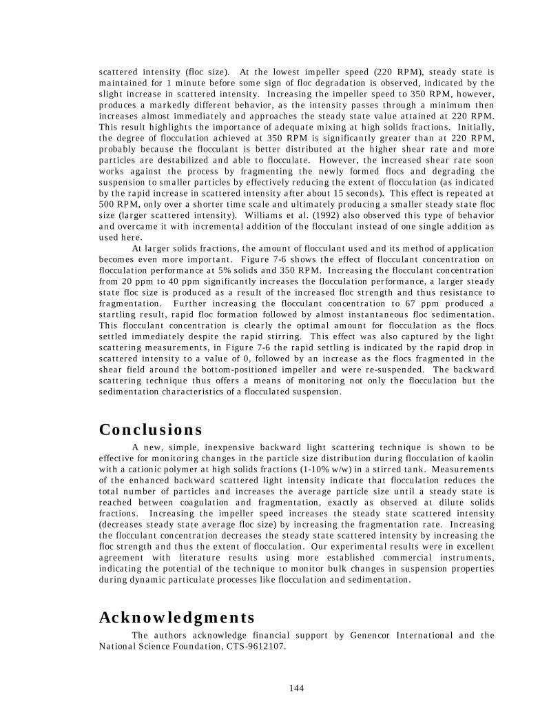
144

scattered intensity (floc size). At the lowest impeller speed (220 RPM), steady state is maintained for 1 minute before some sign of floc degradation is observed, indicated by the slight increase in scattered intensity. Increasing the impeller speed to 350 RPM, however, produces a markedly different behavior, as the intensity passes through a minimum then increases almost immediately and approaches the steady state value attained at 220 RPM. This result highlights the importance of adequate mixing at high solids fractions. Initially, the degree of flocculation achieved at 350 RPM is significantly greater than at 220 RPM, probably because the flocculant is better distributed at the higher shear rate and more particles are destabilized and able to flocculate. However, the increased shear rate soon works against the process by fragmenting the newly formed flocs and degrading the suspension to smaller particles by effectively reducing the extent of flocculation (as indicated by the rapid increase in scattered intensity after about 15 seconds). This effect is repeated at 500 RPM, only over a shorter time scale and ultimately producing a smaller steady state floc size (larger scattered intensity). Williams et al. (1992) also observed this type of behavior and overcame it with incremental addition of the flocculant instead of one single addition as used here. At larger solids fractions, the amount of flocculant used and its method of application becomes even more important. Figure 7-6 shows the effect of flocculant concentration on flocculation performance at 5% solids and 350 RPM. Increasing the flocculant concentration from 20 ppm to 40 ppm significantly increases the flocculation performance, a larger steady state floc size is produced as a result of the increased floc strength and thus resistance to fragmentation. Further increasing the flocculant concentration to 67 ppm produced a startling result, rapid floc formation followed by almost instantaneous floc sedimentation. This flocculant concentration is clearly the optimal amount for flocculation as the flocs settled immediately despite the rapid stirring. This effect was also captured by the light scattering measurements, in Figure 7-6 the rapid settling is indicated by the rapid drop in scattered intensity to a value of 0, followed by an increase as the flocs fragmented in the shear field around the bottom-positioned impeller and were re-suspended. The backward scattering technique thus offers a means of monitoring not only the flocculation but the sedimentation characteristics of a flocculated suspension.

Conclusions A new, simple, inexpensive backward light scattering technique is shown to be effective for monitoring changes in the particle size distribution during flocculation of kaolin with a cationic polymer at high solids fractions (1-10% w/w) in a stirred tank. Measurements of the enhanced backward scattered light intensity indicate that flocculation reduces the total number of particles and increases the average particle size until a steady state is reached between coagulation and fragmentation, exactly as observed at dilute solids fractions. Increasing the impeller speed increases the steady state scattered intensity (decreases steady state average floc size) by increasing the fragmentation rate. Increasing the flocculant concentration decreases the steady state scattered intensity by increasing the floc strength and thus the extent of flocculation. Our experimental results were in excellent agreement with literature results using more established commercial instruments, indicating the potential of the technique to monitor bulk changes in suspension properties during dynamic particulate processes like flocculation and sedimentation.

Acknowledgments The authors acknowledge financial support by Genencor International and the National Science Foundation, CTS-9612107.

145

Notation d particle diameter (µm) t time (s)

Greek Letters φ solids volume fraction (-) ρ particle density (g/cm3) θ angle (degrees)

146

References den Outer, P., “Multiple Light Scattering in Random Discrete Media,” Ph. D. Dissertation,

University of Amsterdam, The Netherlands (1995). Gregory, J. And Gubai, L., “Effects of Dosing and Mixing Conditions on Polymer Flocculation

of Concentrated Suspensions,” Chem. Eng. Comm., 108, 3-21 (1991). Guibai, L. and Gregory, J., "Flocculation and Sedimentation of High-Turbidity Waters,"

Water Research, 25, 1137-1143 (1991). Heffels, C., Willemse, A., Scarlett, B., “Possibilies of Near Backward Light Scattering for

Characterizing Dense Particle Systems,” Powder Tech., 86, 127-135 (1996). Lilge, D. And Horn, D., “Diffusion in Concentrated Dispersions: A Study with Fiber-Optic

Quasi-Elastic Light Scattering (FOQELS),” Colloid Polymer Sci., 269, 704-712 (1991).

Monnier, O., Klein, J.-P., Ratsimba, B., “Particle Size Determination by Laser Reflection: Methodology and Problems,” Part. Part. Sys. Char., 13, 10 (1996).




Serra, T., Colomer, J., Casamitjana, X., “Aggregation And Breakup Of Particles In A Shear Flow.,” J. Colloid Interface Sci., 187, 466 (1997).


Spicer, P. T., Pratsinis, S. E., Trennepohl, M. D., and Meesters, G., “Coagulation and Fragmentation: The Variation of Shear Rate and the Time Lag for Attainment of Steady State,” Ind. Eng. Chem. Res., 35, 3074-3080 (1996).

Wiersma, D. and Lagendijk, A., “Laser Action in Very White Paint,” Physics World, January, 33-37 (1997).

Wiersma, D. S., “Light in Strongly Scattering and Amplifying Random Media,” Ph. D. Dissertation, University of Amsterdam, The Netherlands (1995).

Williams, R. A., Peng, S. J., and Naylor, A., “In situ Measurement of Particle Aggregation and Breakage Kinetics in a Concentrated Suspension,” Powder Tech., 73, 75-83 (1992).

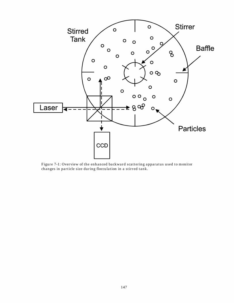
147

Figure 7-1: Overview of the enhanced backward scattering apparatus used to monitor changes in particle size during flocculation in a stirred tank.

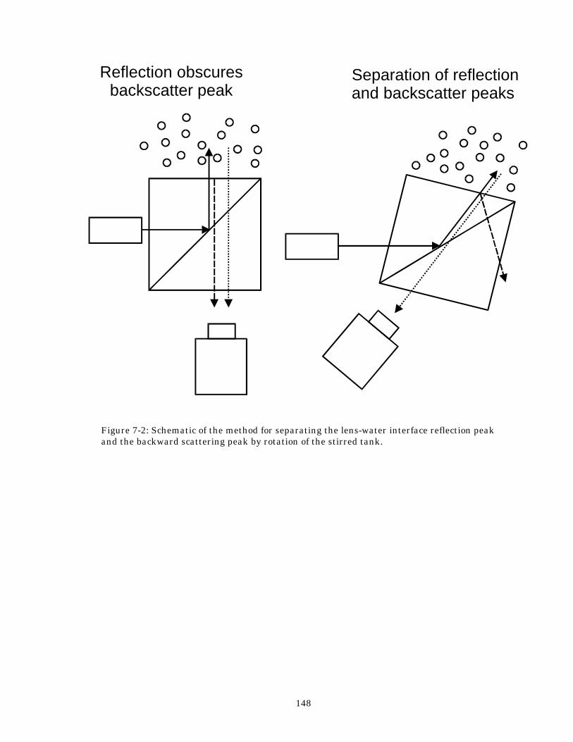
148

Figure 7-2: Schematic of the method for separating the lens-water interface reflection peak and the backward scattering peak by rotation of the stirred tank.

Reflection obscures backscatter peak

Separation of reflectionand backscatter peaks

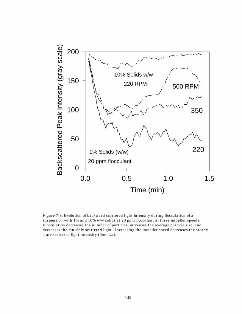
149

Figure 7-3: Evolution of backward scattered light intensity during flocculation of a suspension with 1% and 10% w/w solids at 20 ppm flocculant at three impeller speeds. Flocculation decreases the number of particles, increases the average particle size, and decreases the multiply scattered light. Increasing the impeller speed decreases the steady state scattered light intensity (floc size).

Time (min)

0.0 0.5 1.0 1.5

Bac

ksca

ttere

d P

eak

Inte

nsity

(gr

ay s

cale

)

0

50

100

150

200

500 RPM

350

220

10% Solids w/w

220 RPM

1% Solids (w/w)

20 ppm flocculant

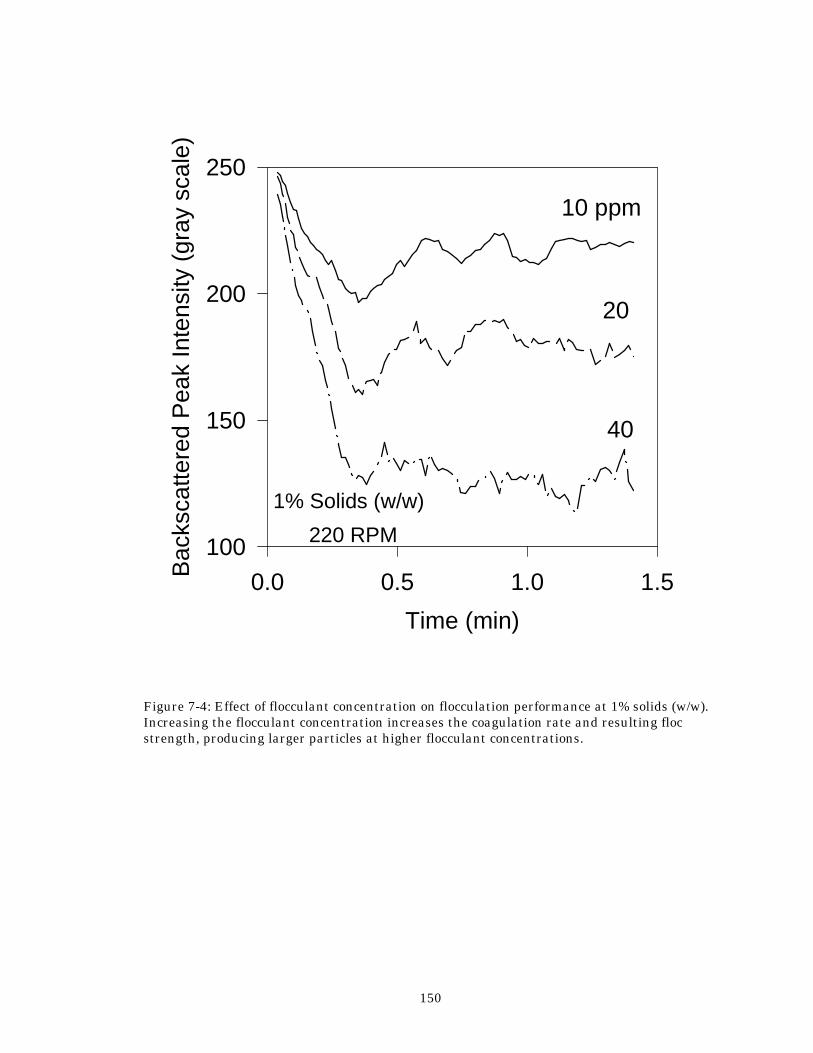
150

Figure 7-4: Effect of flocculant concentration on flocculation performance at 1% solids (w/w). Increasing the flocculant concentration increases the coagulation rate and resulting floc strength, producing larger particles at higher flocculant concentrations.

Time (min)

0.0 0.5 1.0 1.5Bac

ksca

ttere

d P

eak

Inte

nsity

(gr

ay s

cale

)

100

150

200

250

10 ppm

20

40

1% Solids (w/w)

220 RPM

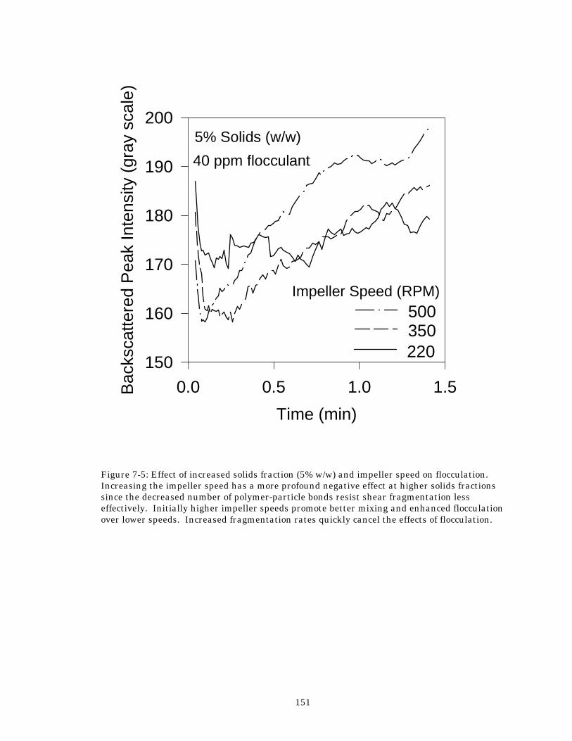
151

Figure 7-5: Effect of increased solids fraction (5% w/w) and impeller speed on flocculation. Increasing the impeller speed has a more profound negative effect at higher solids fractions since the decreased number of polymer-particle bonds resist shear fragmentation less effectively. Initially higher impeller speeds promote better mixing and enhanced flocculation over lower speeds. Increased fragmentation rates quickly cancel the effects of flocculation.

Time (min)

0.0 0.5 1.0 1.5Bac

ksca

ttere

d P

eak

Inte

nsity

(gr

ay s

cale

)

150

160

170

180

190

2005% Solids (w/w)

40 ppm flocculant

220 350500

Impeller Speed (RPM)

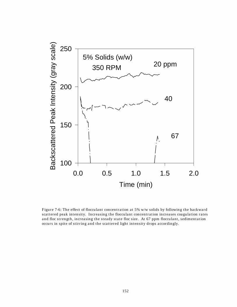
152

Figure 7-6: The effect of flocculant concentration at 5% w/w solids by following the backward scattered peak intensity. Increasing the flocculant concentration increases coagulation rates and floc strength, increasing the steady state floc size. At 67 ppm flocculant, sedimentation occurs in spite of stirring and the scattered light intensity drops accordingly.

Time (min)

0.0 0.5 1.0 1.5 2.0

Bac

ksca

ttere

d P

eak

Inte

nsity

(gr

ay s

cale

)

100

150

200

250

20 ppm

67

40

5% Solids (w/w)350 RPM

153

Chapter 8 - Modeling Shear-Induced Flocculation of Concentrated Suspensions Shear-induced flocculation kinetics of kaolin-polymer flocs are investigated at high solids fractions (φ = 0.01 - 0.1 w/w). Experimental measurements of the floc size distribution are made using two different light backscattering techniques. These results are compared to the predictions of a population balance model describing simultaneous coagulation and fragmentation. As flocculation begins, coagulation dominates and the floc size increases and then levels off at a steady state size as fragmentation becomes significant and balances coagulation. Increasing the shear rate increases the coagulation and fragmentation rates, attaining smaller floc sizes at steady state, but it does not affect the shape or width of the steady state floc size distribution. Increasing the solids fraction increases the coagulation rate, increases the steady state floc size, and broadens the steady state floc size distribution.

154

Introduction From preliminary studies it is clear that at higher solids fractions the larger particle concentration and smaller particle mean free path greatly affects flocculation dynamics. Three dominant deviations from dilute suspension behavior result from the decreased particle mean free path: 1. Multiple particle collisions (greater than binary) 2. Suspension rheology dynamics 3. Mixing-limited flocculant dispersion Clearly there is a need to determine the point at which the dilute theory becomes invalid as a result of one or more of the above factors. The objective of this work is to examine the predictions of existing flocculation theory, valid at dilute volume fractions (φ = 10-6 - 10-3), at higher volume fractions (φ = 0.01 - 0.1) of more relevance to industry. A population balance model is used to predict the effect of increasing solids content on flocculation behavior. The predictions of the model are compared with literature data on the flocculation of kaolin suspensions with a polymer flocculant.

Theory

Population Balance Model The dynamic behavior of the particle size distribution undergoing simultaneous coagulation and fragmentation is given by (Friedlander, 1977; Vigil and Ziff, 1989):

dndt

=12

(u ,u )n n - n (u ,u )n - S n + S ni

j+k=ij k j k i

k=1k i k i i

j=i

imax

j j∑ ∑ ∑∞

αβ αβ γ i j, (8-1)

where ni is the number concentration of flocs of size i (meaning that a single floc contains i primary particles). The first term on the right hand side (RHS) of Equation (8-1) represents the formation of particles comprised of i primary particles by collisions of smaller j- and k-sized particles. The second RHS term denotes the loss of particles of size i by collision with particles of any other size. The third RHS term describes the loss of particles of size i by fragmentation and the fourth RHS term describes the formation of particles of size i by the fragmentation of larger particles. A numerical solution of Equation (8-1) is obtained based on Hounslow et al. (1988) and Kusters et al. (1993) in terms of sections (size classes) of the particle size distribution (Spicer, 1995):

i

j=1

i -2j -i+1

i -1, j i 1 j i -1,i -1 i -12

ij=1

i -1j -i

i, j j

ij=i

i, j j i i i, j j j

imax

dNdt

= 2 N N +12

N - N 2 N

- N N - S N + S N

∑ ∑

∑ ∑

−

=

αβ αβ αβ

αβi

j i

max

Γ

(8-2)

where Ni is the number concentration of flocs of size class i (meaning that a single floc contains 1.5*2i-1 primary particles), α is the collision efficiency for coagulation and βi,k is the collision frequency for particles of size class i and k with characteristic volumes vi and vk, Si is the fragmentation rate of flocs of volume vi, and Γi,j is the breakage distribution function defining the volume fraction of the fragments of size i coming from j-sized particles.

155

The coagulation rate of neutrally buoyant particles smaller than the Kolmogorov microscale, η, in homogeneous, isotropic turbulence is given by (Saffman and Turner, 1956):


+129

1

2 3 (8-3)

where ε is the characteristic turbulent energy dissipation rate of the stirred tank, ν is the kinematic viscosity of the suspending fluid, and ai is the radius of a particle of size i. Equation (8-3) is valid for a solids volume fraction, φ, as large as about 0.1 (Brakalov, 1987). The first term on the RHS of Equation (8-3) in parentheses is the “root mean square velocity gradient”, G, and is frequently used to characterize flocculation processes (Camp and Stein, 1943):

G =

εν

1

2 (8-4)

The rate of fragmentation by splitting of a particle of radius ai is given by (Delichatsios and Probstein, 1976; Kusters, 1991):

Su

au

uii

b=

−

21

2 2

2π∆ ∆

∆exp (8-5)

where ∆u is the rms velocity difference across the distance ai and ∆ub is the critical velocity difference at which breakage of the floc occurs. Substituting into Equation (8-5) for ∆u and ∆ub gives the simplified form of the breakage rate (Kusters, 1991):

Sib=

−

415

12

12

πεν

εε

exp (8-6)

where εb is the critical turbulent energy dissipation rate at which flocs fragment. The εb decreases with increasing floc size as a result of increasing porosity (Tambo and Watanabe, 1979; Sonntag and Russell, 1987; Kusters, 1991):

εb iiad

Ad

( ) = (8-7)

where A and a are fitting parameters. Equation (8-7) describes breakage by a velocity gradient across a droplet or floc and is applicable to droplet breakage at solids fractions as high as 0.5 (Chatzi and Kiparissides, 1995). The flocs are assumed to split upon fragmentation (binary fragmentation) (Chen et al., 1990).

Results and Discussion Figure 8-1 shows the data of Williams et al. (1992) for the evolution of the mass mean

particle length as a function of the shear rate and the solids fraction. In Figure 8-1 the mean floc size increases initially, reaches a maximum, then decreases to a steady state size. The initial maximum is explained as the result of inefficient mixing in the stirred tank, large flocs are produced in segregated regions of the tank and then later fragmented by shear (Gregory, 1991). Another possible explanation is the restructuring of the large flocs produced initially to form more compact structures. Under constant shearing, large open flocs become more compact as the flocs restructure or fragment and reform more durable structures.

156

In Figure 8-1, at a constant solids fraction, an increased shear rate decreases the steady state floc size as a result of the increased fragmentation rate. The growth rate data in Figure 8-1 during the initially coagulation-dominated regime can not be assessed as a result of the lack of resolution in the data. Increasing the solids fraction, φ, decreases the steady state floc size. For a constant flocculant concentration, doubling the initially large solids fraction likely results in the flocculant concentration becoming a limiting factor in the flocculation process. The polymer flocculant acts as a destabilizing agent by occupying surface sites on the particles and either bridging the distance between other particles and/or suppressing the electrostatic repulsion between the particles (Molski, 1989). For a constant flocculant concentration, a substantially increased number of particle surface sites will increase the stability of the suspension, decreasing the efficiency of particle collisions (and thus the coagulation rate) while also possibly increasing the fragmentation rate. Either of these effects will result in a smaller steady state floc size. The modeling approach assumes that all collisions are successful, thus the same effect will not be observed. The evolution of the floc size distribution was simulated by numerical solution of Equation (2-2) including Equations (2-3), (8-6), and (8-7) describing the kinetics of floc growth by collision and fragmentation by shearing. Values of the model parameters φ = 10-2, A = 10-5 a = 2.5, α = 1, d0 = 1 µm, and N0 = 1.91 x 1010 cm-3 were used unless otherwise specified. Figure 8-2 shows the evolution of the mass mean diameter, dmm, calculated with the expression given by Hinds (1982) for various average shear rates, G. The particle size grows rapidly at early times when fragmentation is negligible. After the flocs become larger, however, the growth slows as fragmentation becomes significant. After a characteristic time, the dmm does not change any longer as a result of the dynamic balance between coagulation and fragmentation. This is consistent with the experimental results of Oles (1992) for dilute suspensions as well as that of Gregory and Gubai (1991) and Williams et al. (1992) for concentrated suspensions. Increasing values of G increase the rate of growth during the coagulation-dominated regime (Equation (2-3)), but result in a smaller steady state floc size as a result of the increased fragmentation later on. The combined result of the accelerated coagulation and fragmentation processes is a more rapid attainment of steady state by the suspension (1.75 minutes at G = 10 s-1 versus 0.75 minutes at G = 25 s-1). The effect of solids volume fraction, φ, on the evolution of dmm is shown in Figure 8-3. Increasing φ increases the coagulation rate but does not significantly influence the floc fragmentation rate because collisional breakage is assumed negligible (Glasgow and Luecke, 1980; de Boer et al., 1989; Oles, 1992). In Figure 8-3, increasing φ increases the initial coagulation rate by decreasing the average distance between particles, thus reducing the characteristic time between collisions. A larger floc size is produced at steady state with increasing φ because of the more pronounced effect of φ on the coagulation than the fragmentation rate. The dynamic balance between floc growth and breakage determines the average floc size that is attained at steady state. As a result, increasing the φ increases the coagulation rate to a much greater extent than the fragmentation rate and a larger steady state floc size is reached. The larger φ also results in a faster attainment of steady state than at lower solids fractions because of the accelerated kinetics of both coagulation and fragmentation. This is in excellent qualitative agreement with experimental literature data. Oles (1992) observed steady state time lags on the order of hours for φ = 10-5, whereas Gregory and Gubai (1991) found that flocculating particles reached a steady state at φ = 0.1 in a few minutes. At steady state, the floc size distribution no longer changes as a result of the balance between coagulation and fragmentation. The population balance model allows determination of the effect of the shear rate, G, on the steady state floc size distribution (Figure 8-4a). In Figure 8-4a, the steady state floc size distribution is halted at smaller sizes with increasing G as a result of the increased significance of fragmentation (Equation (8-6)). In spite of the

157

significant effect of shear on the range of the floc size distributions, their shapes are remarkably similar. The steady state floc size distributions in Figure 8-4a are plotted in normalized form in Figure 8-4b to remove the scaling effects of the shear rate, G. Despite the different kinetic behavior at the three different shear rates, the distributions at steady state collapse onto a single curve when scaled by the number average floc volume. This indicates that the final floc size distribution is independent of its initial conditions and can be termed self-preserving with respect to shear. This is in excellent agreement with Spicer and Pratsinis (1996 a, b) who observed this behavior experimentally and theoretically for the flocculation of dilute suspensions of polystyrene particles with aluminum sulfate. In Figure 8-5b the steady state size distribution is plotted as a function of the solids volume fraction, φ. Increasing the φ produces a broader floc size distribution at steady state because the coagulation and fragmentation rates are both enhanced at larger solids fractions. The floc size distribution is halted at a larger size range because the increased solids fraction enhances the coagulation rate more significantly than the fragmentation rate. This is seen more clearly in Figure 8-5b, which shows the effect of solids fraction on the steady state floc size distributions in Figure 8-5a after scaling with the average floc size. In Figure 8-5b, increasing the φ extends the floc size distribution into the larger floc sizes to a greater extent than into the smaller sizes. This is because of the greater enhancement of the coagulation rate by the solids fractions versus that of the fragmentation rate.

Conclusions A population balance model was used to theoretically describe the flocculation of spherical particles at large solids fractions (φ = 0.01-0.02). An increased shear rate, G, increases the coagulation rate, decreases the steady state average floc size, but does not influence the shape of the steady state floc size distribution. Increasing the solids fraction, φ, increases the coagulation rate and the steady state floc size but broadens the steady state floc size distribution significantly. The model is in good agreement with the existing limited experimental data on the flocculation of concentrated solids suspensions.

Acknowledgments Financial support by Genencor International B. V. is gratefully acknowledged.

158

Notation a particle radius (µm) A breakage rate coefficient (cm-3a s-1) a power law exponent, breakage rate (-) aI radius of particle with index i (µm) d0 primary particle diameter (µm) dmm mass mean particle diameter (µm) G spatially averaged shear rate (s-1) N0 initial number concentration (# / cm3) ni discrete number concentration of particles with index i (# / cm3) Ni sectional number concentration of particles with index i (# / cm3) Si particle fragmentation rate (s-1) t time (s) u fluid velocity (cm/s)

ub critical breakage velocity (cm/s)

Greek Letters α collision efficiency (-) β i,j collision frequency (cm3/s) γ i,j discrete fragment size distribution of size i fragments (-) Γ i,j sectional fragment size distribution of size i fragments (-) ε energy dissipation rate (cm2/s3) εb critical fragmentation energy dissipation rate (cm2/s3) φ solids volume fraction (-) η Kolmogorov microscale (µm) ν kinematic viscosity (cm2 / s)

159

References Brakalov, L. B., “A Connection Between the Orthokinetic Coagulation Capture Efficiency of

Aggregates and their Maximum Size,” Chem Eng. Sci., 42, 2373-2383 (1987). Camp, T. R. and Stein, P. G., "Velocity Gradients and Internal Work in Fluid Motion," J.

Boston Soc. Civ. Eng., 30, 219, (1943). Chatzi, E. G. and Kiparisssides, C., “Steady-State Drop-Size Distributions in High Holdup

Fraction Dispersion Systems,” AIChE J., 41, 1640-1652 (1995). Chen, W., Fisher, R. R., Berg, J. C., "Simulation of Particle Size Distribution in an

Aggregation-Breakup Process," Chem. Eng. Sci., 45, 3003-3006 (1990). Clark, M. M., “Critique of Camp and Stein’s RMS Velocity Gradient,” J. Env. Eng., 111, 741-

754 (1985). de Boer, G. B. J., Hoedemakers, G. F. M., and Thoenes, D., “Coagulation in Turbulent Flow:

Part I,” Chem. Eng. Res. Des., 67, 301-307 (1989). Delichatsios, M. A., and Probstein, R. F., "The Effect of Coalescence on the Average Drop Size

in Liquid-Liquid Dispersions," Ind. Eng. Chem., Fund., 15, 134-138 (1976). Friedlander, S. K., Smoke, Dust, and Haze, Wiley, New York, (1977). Glasgow, L. A. and Luecke, R. H., “Mechanisms of Deaggregation for Clay-Polymer Flocs in

Turbulent Systems,” Ind. Eng. Chem. Fundam., 19, 148-156 (1980). Gregory, J., “Effect of Dosing and Mixing Conditions on Flocculation by Polymers,” in


Gregory, J. And Gubai, L., “Effects of Dosing and Mixing Conditions on Polymer Flocculation of Concentrated Suspensions,” Chem. Eng. Comm., 108, 3-21 (1991).

Guibai, L. and Gregory, J., "Flocculation and Sedimentation of High-Turbidity Waters," Water Research, 25, 1137-1143 (1991).

Hinds, W. C., Aerosol Technology, Wiley-Interscience, New York (1982). Hounslow, M. J., Ryall, R. L., and Marshall, V. R., "A Discretized Population Balance for

Nucleation, Growth, and Aggregation," AIChE J., 34, 1821-1832 (1988). Kusters, K. A., "The Influence of Turbulence on Aggregation of Small Particles in Agitated

Vessels," Ph. D. Thesis, Eindhoven University of Technology, The Netherlands, (1991).

Kusters, K. A., Pratsinis, S. E., Thoma, S. G., and Smith, D. M., “Ultrasonic Fragmentation of Agglomerate Powders,” Chem. Eng. Sci., 48, 4119-4127 (1993).

Molski, A., "On the Collision Efficiency Approach to Flocculation," Colloid and Polym. Sci., 267, 371-375 (1989).





Spicer, P. T., “The Dynamics of Shear-Induced Flocculation in a Stirred Tank,” M.S. Thesis, University of Cincinnati, Cincinnati, OH (1995).

Tambo, N. and Watanabe, Y., "Physical Characteristic of Flocs: I. The Floc Density Function and Aluminum Floc," Water Res., 13, 409-419 (1979).

Vigil, R. D. and Ziff, R. M., "On the Stability of Coagulation-Fragmentation Population Balances," J. Colloid Interface Sci., 133, 257-264 (1989).

Williams, R. A., Peng, S. J., and Naylor, A., “In situ Measurement of Particle Aggregation and Breakage Kinetics in a Concentrated Suspension,” Powder Tech., 73, 75-83 (1992).

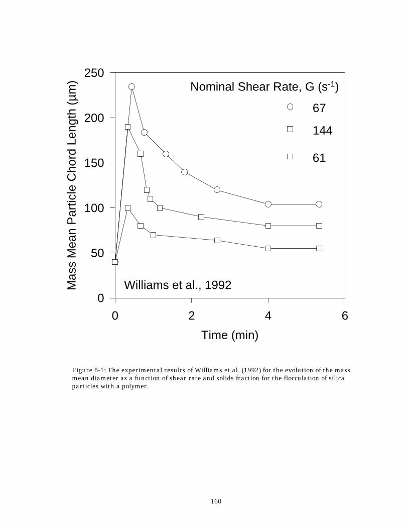
160

Figure 8-1: The experimental results of Williams et al. (1992) for the evolution of the mass mean diameter as a function of shear rate and solids fraction for the flocculation of silica particles with a polymer.

Time (min)

0 2 4 6

Mas

s M

ean

Par

ticle

Cho

rd L

engt

h (µ

m)

0

50

100

150

200

250

Williams et al., 1992

Nominal Shear Rate, G (s-1)

67

144

61

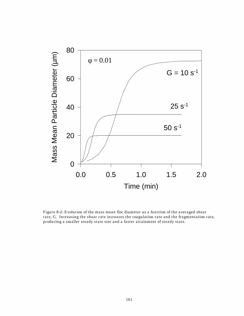
161

Figure 8-2: Evolution of the mass mean floc diameter as a function of the averaged shear rate, G. Increasing the shear rate increases the coagulation rate and the fragmentation rate, producing a smaller steady state size and a faster attainment of steady state.

Time (min)

0.0 0.5 1.0 1.5 2.0

Mas

s M

ean

Par

ticle

Dia

met

er (

µm)

0

20

40

60

80φ = 0.01

G = 10 s-1

25 s-1

50 s-1

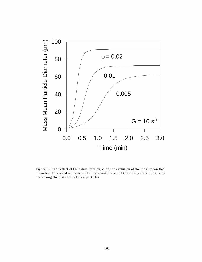
162

Figure 8-3: The effect of the solids fraction, φ, on the evolution of the mass mean floc diameter. Increased φ increases the floc growth rate and the steady state floc size by decreasing the distance between particles.

Time (min)

0.0 0.5 1.0 1.5 2.0 2.5 3.0

Mas

s M

ean

Par

ticle

Dia

met

er (

µm)

0

20

40

60

80

100

φ = 0.02

G = 10 s-1

0.01

0.005

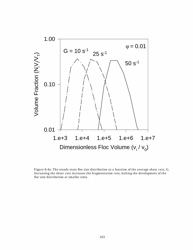
163

Figure 8-4a: The steady state floc size distribution as a function of the average shear rate, G. Increasing the shear rate increases the fragmentation rate, halting the development of the floc size distribution at smaller sizes.

Dimensionless Floc Volume (vi / v0)

1.e+3 1.e+4 1.e+5 1.e+6 1.e+7

Vol

ume

Fra

ctio

n (N

iVi/V

T)

0.01

0.10

1.00φ = 0.01

G = 10 s-125 s-1

50 s-1

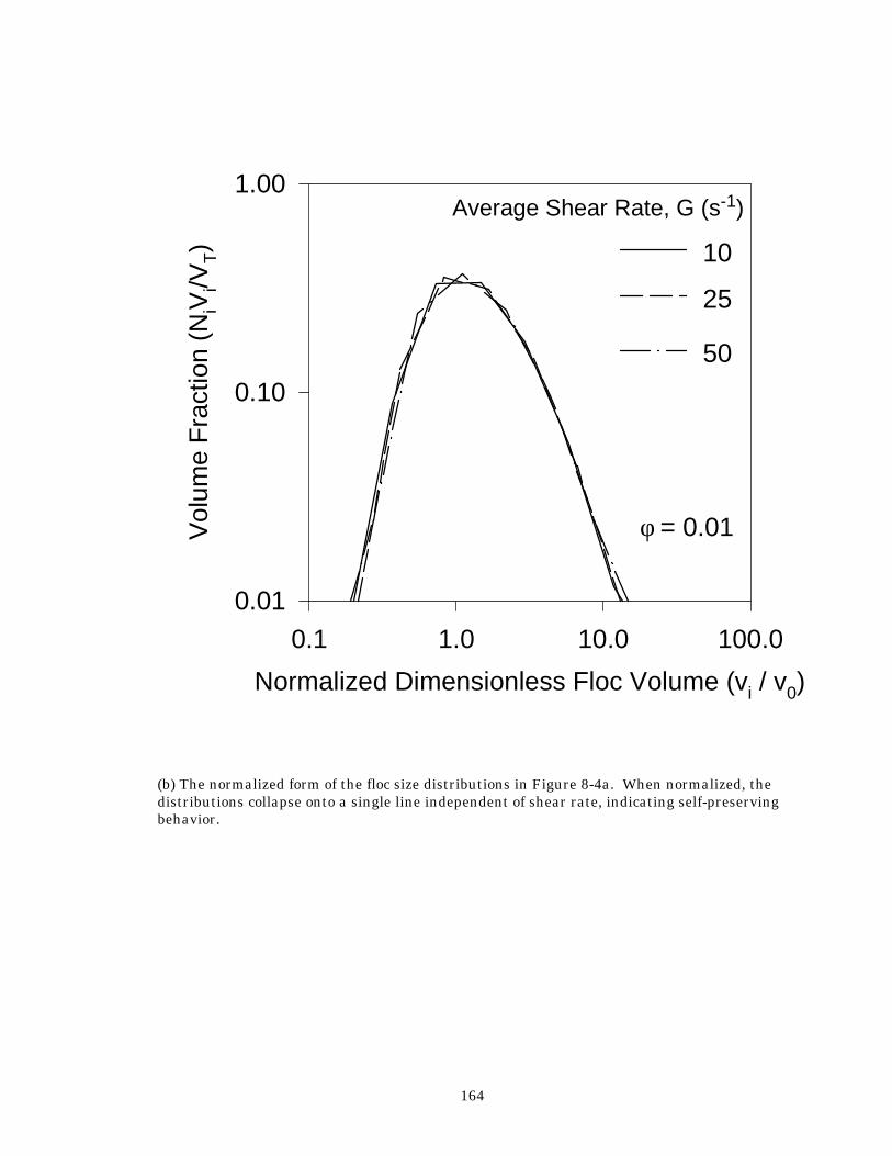
164

(b) The normalized form of the floc size distributions in Figure 8-4a. When normalized, the distributions collapse onto a single line independent of shear rate, indicating self-preserving behavior.

Normalized Dimensionless Floc Volume (vi / v0)

0.1 1.0 10.0 100.0

Vol

ume

Fra

ctio

n (N

iVi/V

T)

0.01

0.10

1.00

φ = 0.01


10

25

50

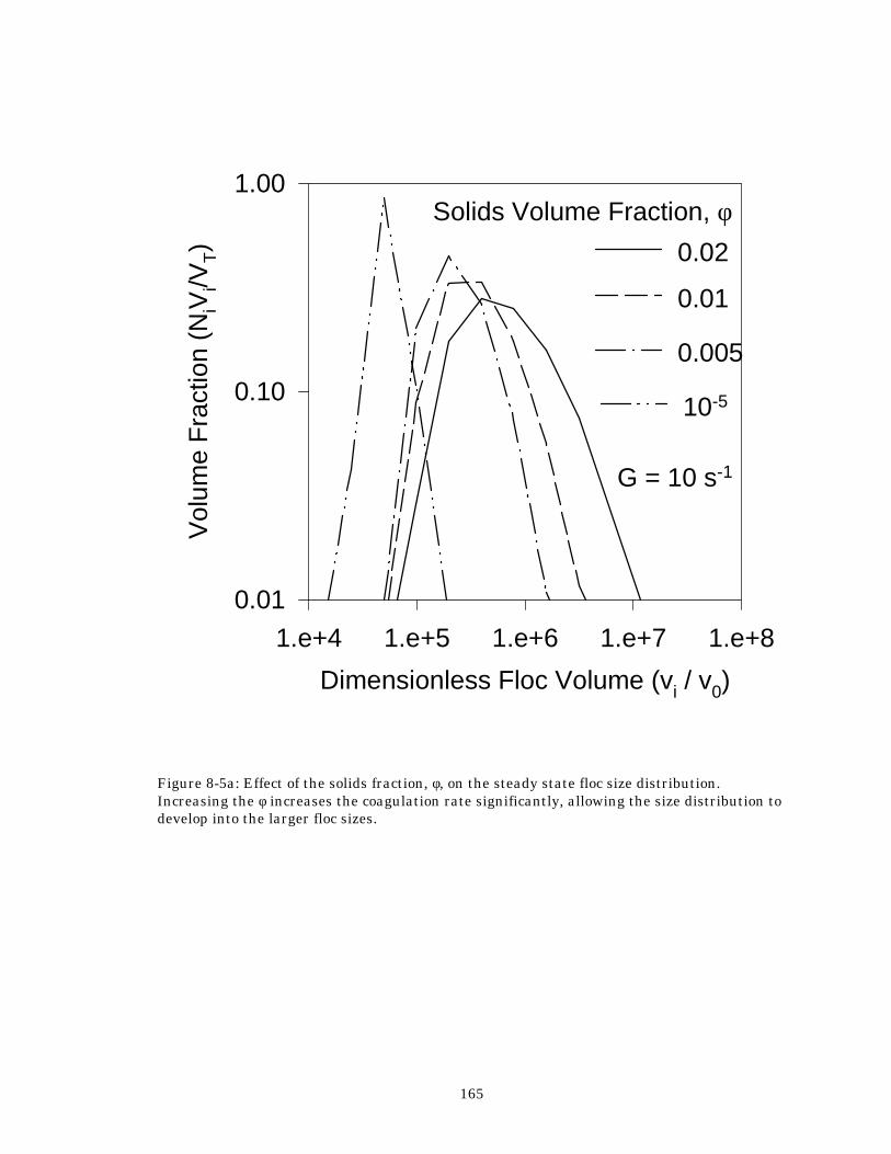
165

Figure 8-5a: Effect of the solids fraction, φ, on the steady state floc size distribution. Increasing the φ increases the coagulation rate significantly, allowing the size distribution to develop into the larger floc sizes.

Dimensionless Floc Volume (vi / v0)

1.e+4 1.e+5 1.e+6 1.e+7 1.e+8

Vol

ume

Fra

ctio

n (N

iVi/V

T)

0.01

0.10

1.00Solids Volume Fraction, φ

G = 10 s-1

0.02

0.01

0.005

10-5

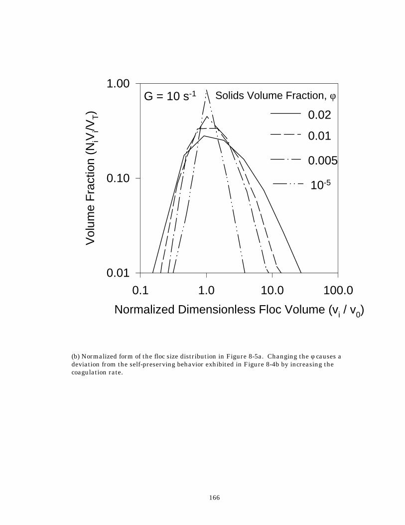
166

(b) Normalized form of the floc size distribution in Figure 8-5a. Changing the φ causes a deviation from the self-preserving behavior exhibited in Figure 8-4b by increasing the coagulation rate.

Normalized Dimensionless Floc Volume (vi / v0)

0.1 1.0 10.0 100.0

Vol

ume

Fra

ctio

n (N

iVi/V

T)

0.01

0.10

1.00Solids Volume Fraction, φG = 10 s-1

0.02

0.01

0.005

10-5

167

Conclusions / Suggestions for Future Work The results obtained in this dissertation highlight the importance of three factors during shear-induced aggregation of particles in a liquid. Each of these factors has been shown to have significant effects on aggregation kinetics, although much work remains before a complete picture exists.

Increasingly irregular, fractal aggregate structures exhibit accelerated growth and destruction when exposed to fluid shear. The viscous resistance to particle-particle collisions is decreased as a result of the porous morphology of fractal aggregates, further enhancing collision frequencies. Aggregate structure is poorly characterized by idealized simulations, although the incorporation of realistic processes like sintering and restructuring into such simulations may compensate for these inaccuracies. In certain shear environments, such as rotational flow, fractal aggregates may approach spherical behavior, easing the computational load during simulations of suspension flow. More research is needed to determine the best means of simulating fractal aggregate formation and dynamics in order to more closely approximate and engineer the physical world.

The fluid flow field driving shear-induced aggregation can accelerate both particle coagulation and fragmentation if the local velocity gradient is increased. The similarities between laminar and turbulent shear are often blurred during aggregation processes, although the length scale under consideration is a crucial factor. Aggregation in heterogeneous flow fields like those found in stirred tanks are difficult to describe theoretically because of the dearth of knowledge regarding the effect of process variables on mixing rates. More research is needed into experimental tools for fluid flow characterization as well as reliable theoretical simulations. The merging of the computational fluid dynamic (CFD) models with particle dynamics models will bring a new generation of theories to light.

Solids concentration alters the particle mean free path in a suspension, vastly accelerating aggregation and fragmentation rates. The limits of current theoretical and experimental tools have been reached and the need for more robust techniques is obvious. Reliable means of directly monitoring particle size distribution dynamics in a concentrated suspension are needed in order to validate developing theories regarding the multiple body interactions occurring in a high solids suspension.

168

Yes, there’s still more…

Appendices 1-9

169

Appendix 1: Chapter 2 Computer Code

c CFS.FOR Model of Litster et al. (1995) for sectional coagulation c and fragmentation using the kernel for shear coagulation c given by Saffman and Turner (1956) and assuming binary fragmentation c implicit double precision (a-h,n-z) implicit integer*4(i-m) c dimension y(50),yp(50),v(50),b(50),beta(50,50) dimension s(50),wk(10000),iwk(10000) c common /basic/beta,max,tmax,xn0,v0,d0,df,v,b,s,mq,volumei,voldif common /basic2/g,phi,tau common /distr/sumofn,sumofnv,sigmagn,sigmagv common /break/xba,biga c external fcn,fcnj,dgear c open (unit = 3, file = 'dist.prn') open (unit = 4, file = 'spdist.prn') open (unit = 5, file = 'sigma.prn') open (unit = 7, file = 'n.prn') open (unit = 8, file = 'nv.prn') open (unit = 2, file = 'cfs.dat', status = 'old') c read(2,*) xn0 read(2,*) d0 read(2,*) tmax read(2,*) max read(2,*) tol read(2,*) h read(2,*) xfactor read(2,*) mq read(2,*) g read(2,*) xba1 read(2,*) xba2 read(2,*) df c xba = xba1/xba2 c c Physical constants c rkb = 1.38066d-16 vpi = 3.1415927d0 c c dgear parameters c imeth = 1 imiter = 0 index = 1 ier = 0 t = 0.d0

170

tend = 0.d0 ieq = max c c Calculate v0 (cm3) c v0 = (vpi*d0**3.d0)/6.d0 c c Phi (volume fraction) c phi = xn0*v0 c c sectional spacing factor (factor), boundaries of sections (b), c characteristic volumes vi/v0 (v), number concentrations (y) c factor = 2.d0**(1.d0/mq) b(0) = 1.d0 c do 100 k=1,max b(k) = factor*b(k-1) v(k) = (b(k)+b(k-1))/2.d0 y(k) = 0.d0 100 continue c y(1) = xn0 c c Sum initial volume concentration c volumei = 0.d0 do 200 i = 1,max volumei = volumei+v(i)*y(i) 200 continue c call shear c call split c c --------------------------------------------------- c Loop to execute dgear for specified time period c 500 tend = t + tmax/xfactor call dgear(ieq,fcn,fcnj,t,h,y,tend,tol,imeth, 1 imiter,index,iwk,wk,ier) c call output(y,t) call loss(y) write(6,525)tau,sigmagn,sigmagv 525 format (5(1x,e12.6)) c if(tend.lt.tmax) goto 500 c ---------------------------------------------------- c Write final size distributions to files c call sp(y) c c Write final volume loss to screen c

171

call loss(y) 600 stop end c---------------------------------------------------------------------- c subroutine to calculate volume and number loss c subroutine loss(y) implicit double precision (a-h,n-z) implicit integer*4(i-m) dimension y(50),v(50),beta(50,50),b(50),s(50) common /basic/beta,max,tmax,xn0,v0,d0,df,v,b,s,mq,volumei,voldif common /distr/sumofn,sumofnv,sigmagn,sigmagv external sumn,sumv c call sumn(y,t) call sumv(y,t) c voldif = (volumei - sumofnv)/volumei xnumdif = (xn0 - sumofn)/xn0 c return end c------------------------------------------------------------------------ c Calculate summation of indices c function ms(i) implicit double precision (a-h,n-z) implicit integer*4(i-m) c ms = i*(i + 1)/2 c return end c---------------------------------------------------------------------- c differential equations to be solved c---------------------------------------------------------------------- subroutine fcn(ieq,t,y,yp) implicit double precision (a-h,n-z) implicit integer*4(i-m) dimension y(50),yp(50),beta(50,50),v(50),b(50),s(50) common /basic/beta,max,tmax,xn0,v0,d0,df,v,b,s,mq,volumei,voldif common /distr/sumofn,sumofnv,sigmagn,sigmagv common /basic2/g,phi,tau external ms,shear,split c g = 30.d0*sin(t) + 50.0001d0 call shear call split c c Sectional model of Litster et al., 1994 c do 9000 i = 1,max c if(y(i).lt.0.d0) y(i) = 0.d0 c c First Term

172

c sum10 = 0.d0 if (i - ms(mq) - 1.lt.1) goto 1100 do 1000 j = 1,i - ms(mq) - 1 eks1 = 2.d0**((j - i + 1)/dfloat(mq)) eks2 = 2.d0**(1.d0/mq) - 1.d0 twofact1 = (eks1/eks2) sum10 = sum10+beta(i-1,j)*y(i-1)*y(j)*twofact1 1000 continue c c Second Term c 1100 sum11 = 0.d0 if (mq.eq.1) goto 1400 do 1300 k = 2,mq if (i-ms(mq-k+1)-k.lt.1) goto 1300 do 1200 j = i-ms(mq-k+2)-k+1,i-ms(mq-k+1)-k if (j.ge.1.and.i-k.ge.1) then pts1 = 2.d0**((j-i+1)/dfloat(mq))-1.d0 pts2 = 2.d0**(-(k-1)/dfloat(mq)) pts3 = 2.d0**(1.d0/mq)-1.d0 twofact2 = (pts1+pts2)/pts3 sum11 = sum11+beta(i-k,j)*y(i-k)*y(j)*twofact2 endif 1200 continue 1300 continue c c Third Term c 1400 sum12 = 0.d0 if(i-mq.lt.1) goto 1500 sum12 = 0.5d0*beta(i-mq,i-mq)*y(i-mq)*y(i-mq) c c Fourth Term c 1500 sum13 = 0.d0 if (mq.eq.1) goto 1750 do 1700 k = 2,mq if (i-ms(mq-k+1)-k+1.lt.1) goto 1700 do 1600 j = i-ms(mq-k+2)-k+2,i-ms(mq-k+1)-k+1 if (j.ge.1.and.i-k+1.ge.1) then pat1 = -2.d0**((j-i)/dfloat(mq)) pat2 = 2.d0**(1.d0/mq)-2.d0**(-(k-1)/dfloat(mq)) pat3 = 2.d0**(1.d0/mq)-1.d0 twofact3 = (pat1+pat2)/pat3 sum13 = sum13+beta(i-k+1,j)*y(i-k+1)*y(j)*twofact3 endif 1600 continue 1700 continue c c Fifth Term c 1750 sum14 = 0.d0 if (i-ms(mq).lt.1) goto 1900 do 1800 j = 1,i-ms(mq) cls1 = 2.d0**((j-i)/dfloat(mq))

173

cls2 = 2.d0**(1.d0/mq)-1.d0 twofact4 = cls1/cls2 sum14 = sum14+beta(i,j)*y(i)*y(j)*twofact4 1800 continue c c Sixth Term c 1900 sum15 = 0.d0 do 2000 j = i-ms(mq)+1,max if (j.ge.1) then sum15 = sum15 + beta(i,j)*y(i)*y(j) endif 2000 continue c c Coagulation Term c coag = sum10+sum11+sum12+sum13-sum14-sum15 c c Fragmentation Term (Binary Breakage Only) c frag = 2.d0*s(i+1)*y(i+1) - s(i)*y(i) c c Sum terms of population balance c 2100 yp(i) = coag + frag c 9000 continue return end c----------------------------------------------------------------- c dummy routine for dgear c subroutine fcnj (n,x,y,pd) integer n real *8 x,y,pd(10,10) return end c------------------------------------------------------------------ subroutine output(y,t) implicit double precision (a-h,n-z) implicit integer*4(i-m) dimension v(50),y(50),beta(50,50),b(50),s(50) common /basic/beta,max,tmax,xn0,v0,d0,df,v,b,s,mq,volumei,voldif common /distr/sumofn,sumofnv,sigmagn,sigmagv common /basic2/g,phi,tau external sumn,sumv c call sumn(y,t) call sumv(y,t) c c Landgrebe's formulae for parameters c c V-based parameters c vgsum = 0.d0 do 3011 i = 1,max

174

d1 = b(i)*log(b(i))-b(i-1)*log(b(i-1)) d2 = b(i)-b(i-1) vgsum = vgsum+(y(i)*v(i)*(d1/d2-1.d0))/sumofnv 3011 continue vgv = exp(vgsum) c sigsum = 0.d0 do 3013 i = 1,max factor1 = b(i)*log(b(i)/vgv)**2.d0-b(i-1)*log(b(i-1)/vgv)**2.d0 factor2 = b(i)*log(b(i))-b(i-1)*log(b(i-1)) factor3 = b(i)-b(i-1) combin = (factor1-2.d0*factor2)/factor3 sigsum = sigsum+y(i)*v(i)*(combin+2.d0*(1.d0+log(vgv)))/sumofnv 3013 continue sigmagv = dsqrt(sigsum/9.d0) sigmagv = dexp(sigmagv) c c N-Based parameters c vgsum = 0.d0 do 3050 i = 1,max d1 = b(i)*log(b(i))-b(i-1)*log(b(i-1)) d2 = b(i)-b(i-1) vgsum = vgsum+(y(i)*(d1/d2-1.d0))/sumofn 3050 continue vgn = exp(vgsum) c sigsum = 0.d0 do 3075 i = 1,max factor1 = b(i)*log(b(i)/vgn)**2.d0-b(i-1)*log(b(i-1)/vgn)**2.d0 factor2 = b(i)*log(b(i))-b(i-1)*log(b(i-1)) factor3 = b(i)-b(i-1) combin = (factor1-2.d0*factor2)/factor3 sigsum = sigsum+y(i)*(combin+2.d0*(1.d0+log(vgn)))/sumofn 3075 continue sigmagn = dsqrt(sigsum/9.d0) sigmagn = dexp(sigmagn) c c Mass Mean Diameter (Kusters, 1991) c vpi = 3.14159d0 dsum1 = 0.d0 dsum2 = 0.d0 do 3232 i = 1,max di = (6.d0*v(i)*v0/vpi)**(1.d0/3.d0) dsum1 = dsum1 + y(i)*di**4.d0 dsum2 = dsum2 + y(i)*di**3.d0 3232 continue xmmd = dsum1/dsum2 c c Dimensionless time (Oles, 1992) c tau = g*phi*t c c output parameters c

175

ee = sumofn ev = sumofnv write(5,3800)t/3.6d3,tau,sigmagn,sigmagv,xmmd/d0 write(7,3801) t/3.6d3,tau,y(1)/ee,y(2)/ee,y(3)/ee write(8,3802) t/3.6d3,tau,y(1)*v(1)/ev,y(2)*v(2)/ev,y(3)*v(3)/ev 3800 format(5(1x,e12.6)) 3801 format(4(1x,e12.6)) 3802 format(4(1x,e12.6)) c return end c------------------------------------------------------------------- c Calculate distributions c subroutine sp(y) implicit double precision (a-h,n-z) implicit integer*4(i-m) dimension y(50),b(50),s(50),v(50),beta(50,50) common /basic/beta,max,tmax,xn0,v0,d0,df,v,b,s,mq,volumei,voldif common /distr/sumofn,sumofnv,sigmagn,sigmagv external sumn,sumv c call sumn(y,t) call sumv(y,t) c vavg = sumofnv/sumofn c do 4500 j = 1,max write(3,4750) v(j),y(j)/sumofn,y(j)*v(j)/sumofnv write(4,4755) v(j)/vavg,y(j)/sumofn,y(j)*v(j)/sumofnv 4500 continue 4750 format(3(1x,e12.6)) 4755 format(3(1x,e12.6)) c return end c------------------------------------------------------------------- subroutine sumn(y,t) implicit double precision (a-h,n-z) implicit integer*4(i-m) dimension y(50),b(50),s(50),v(50),beta(50,50) common /basic/beta,max,tmax,xn0,v0,d0,df,v,b,s,mq,volumei,voldif common /distr/sumofn,sumofnv,sigmagn,sigmagv c sumofn = 0.d0 do 5020 k = 1,max sumofn = sumofn + y(k) 5020 continue c return end c------------------------------------------------------------------- subroutine sumv(y,t) implicit double precision (a-h,n-z) implicit integer*4(i-m) dimension y(50),b(50),s(50),v(50),beta(50,50)

176

common /basic/beta,max,tmax,xn0,v0,d0,df,v,b,s,mq,volumei,voldif common /distr/sumofn,sumofnv,sigmagn,sigmagv c sumofnv = 0.d0 do 5030 k = 1,max sumofnv = sumofnv + y(k)*v(k) 5030 continue c return end c---------------------------------------------------------------------- c Calculate shear coagulation kerne subroutine shear implicit double precision (a-h,n-z) implicit integer*4(i-m) dimension y(50),b(50),s(50),v(50),beta(50,50) common /basic/beta,max,tmax,xn0,v0,d0,df,v,b,s,mq,volumei,voldif common /basic2/g,phi,tau common /distr/sumofn,sumofnv,sigmagn,sigmagv c r0 = d0/2.d0 do 400 i = 1,max do 300 j = 1,max a1 = r0*v(i)**(1.d0/df) a2 = r0*v(j)**(1.d0/df) beta(i,j) = 1.3d0*g*(a1 + a2)**3.d0 300 continue 400 continue c return end c---------------------------------------------------------------------- c Calculate fragmentation rate subroutine split implicit double precision (a-h,n-z) implicit integer*4(i-m) dimension y(50),b(50),s(50),v(50),beta(50,50) common /basic/beta,max,tmax,xn0,v0,d0,df,v,b,s,mq,volumei,voldif common /basic2/g,phi,tau common /distr/sumofn,sumofnv,sigmagn,sigmagv common /break/xba,biga c biga = 0.0047d0*(g**1.6d0) c s(1) = 0.d0 do 410 k = 2,max s(k) = biga*((v0*v(k))**(xba)) 410 continue return end

177

Appendix 2: Chapter 5 Computer Code (Simulation) cccccccccccccccccccccccccccccccccccccccccccccccccccccccccccccccccccccccccccccccccccc c c CCAT.FOR Monte Carlo simulation of Cluster-Cluster Aggregation using a tunable Df c by the technique of Thouy and Jullien, 1994. c cccccccccccccccccccccccccccccccccccccccccccccccccccccccccccccccccccccccccccccccccccc program ccat use msimsl implicit real*8(a-h,n-z) implicit integer*4(i-m) parameter (maxind = 9000) common /coords/ mx(9000),my(9000),mz(9000) common /fracds/ neighb(50),surfsits(50) common /neighb/ mtotn,mnx(9000),mny(9000),mnz(9000) common /params/ mexp common /sizes/ dcav(50),rgav(50) common /surfac/ mtots,mns(9000) dimension dgam(9000),dgams(9000),igdx(9000),igdy(9000),igdz(9000) dimension iperm(9000) logical ovrlap,dgaml(9000) external ran1 c open (unit = 3, file = 'ccatune.in') open (unit = 4, file = 'xyz.prn') open (unit = 5, file = 'nrg.prn') open (unit = 7, file = 'fractal.scr') c call outtim(0) c Initialize the random number generator (negative integer less than -2) read(3,*) idum c Input value of fractal dimension, Df, desired for aggregate read(3,*) delta c Set the initial number of particles read(3,*) mexp c Read tolerance for comparison of optimal orientations read(3,*) dgmtol c Initialize primary particle coordinate arrays mx = 0 my = 0 mz = 0 c Initialize indices of reference and collider particles ira0 = 1 irb0 = 1 ica0 = 2 icb0 = 2 ira = ira0 irb = irb0 ica = ica0 icb = icb0 mm = mexp - 1 c This section pairs the primary particles for each hierarchical step

178

do m = 1,mexp rga = 0.d0 dca = 0.d0 neigha = 0.d0 surfa = 0.d0 do i = 1,2**(mm) c-----Between these comments the indices change consistently---------------------- c Initialize orientation parameters igam = 0 dgam = 1.d6 dgaml = .false. dgm = 1.d6 iperm = (/(ip, ip = 1,9000)/) c Count neighbor sites of reference call nbrcnt(ira,irb) c Count surface particles of collider call surcnt(ica,icb) c Orient colliding aggregate's chosen surface particle at c all neighbor sites of the reference particle do k = 1,mtots do kk = 1,mtotn if (igam.eq.1000) cycle c Find change in coordinates based on current surface particle idx = mnx(kk) - mx(mns(k)) idy = mny(kk) - my(mns(k)) idz = mnz(kk) - mz(mns(k)) c Assign new, temporary coordinates of collider do j = ica,icb mx(j) = mx(j) + idx my(j) = my(j) + idy mz(j) = mz(j) + idz enddo c Check for overlap of other particles and determine structure if(.not.ovrlap(ira,icb)) then c Actual structure call com(ira,irb,rx,ry,rz) call com(ica,icb,cx,cy,cz) gamma2 = db2(rx,ry,rz,cx,cy,cz)**2.d0 c Desired structure rg1 = rg(ira,irb) rg2 = rg(ica,icb) xk2 = 4.d0*(4.d0**(1.d0/delta) - 1.d0) g2 = (rg1 + rg2)*xk2/2.d0 + 1.d0 c Deviation from desired structure dg = (gamma2 - g2)**2.d0 c If new minimum found, start count over if (dg.lt.dgm) then igam = 0 c Assign local minimum deviation dgm = dg endif c Only record deviation if small enough if (abs(dg - dgm).le.1.d-4*dgm) then c Record interpenetration and corresponding delta coordinates igam = igam + 1

179

dgam(igam) = dg igdx(igam) = idx igdy(igam) = idy igdz(igam) = idz endif endif c Reassign original coordinates for next loop do j = ica,icb mx(j) = mx(j) - idx my(j) = my(j) - idy mz(j) = mz(j) - idz enddo enddo if (igam.eq.1000) cycle enddo c Alert if no dgs meet criteria if (igam.eq.0) write(6,*)'igam = 0!' c Determine minimum dgamma by sorting the array into ascending order call dsvrbp(9000,dgam,dgams,iperm) dgm = dgams(1) c Mark minimum dgamma occurrences where (abs(dgam - dgm).le.dgmtol*dgm) dgaml = .true. end where c Count occurrences of minimum dgamma dgmcnt = count(dgaml) c Randomly choose one of the minimum orientations igmrnd = int(dgmcnt*ran1(idum) + 1) c Reorient collider at new position do ii = ica,icb mx(ii) = mx(ii) + igdx(iperm(igmrnd)) my(ii) = my(ii) + igdy(iperm(igmrnd)) mz(ii) = mz(ii) + igdz(iperm(igmrnd)) enddo c Calculate average radius of gyration rga = rga + rg(ira,icb)/dfloat(2**(mexp - m)) rgav(m) = rga c Calculate average collision diameter dca = dca + dc(ira,icb)/dfloat(2**(mexp - m)) dcav(m) = dca c Count neighbor sites of resultant aggregate call nbrcnt(ira,icb) c Count surface particles of resultant aggregate call surcnt(ira,icb) c Calculate average number of neighbor surface sites neigha = neigha + mtotn/dfloat(2**(mexp - m)) neighb(m) = neigha c Calculate average number of surface particles surfa = surfa + mtots/dfloat(2**(mexp - m)) surfsits(m) = surfa c--------------------------------------------------------------------------------- ira = ira + 2**m irb = irb + 2**m ica = ica + 2**m icb = icb + 2**m if(i.eq.2**mm) then

180

mm = mm - 1 ira = ira0 irb = 2**m ica = ica0 + 2**(m-1) icb = 2**(m+1) ica0 = ica endif enddo c Calculate estimate of fractal dimension if (m.gt.1) then df = dlog(4.d0)/(dlog(rgav(m) - 0.25d0) - dlog(rgav(m-1))) else df = 0 endif write(6,1200)2**m,df 1200 format(i4,3(1x,e12.6)) enddo c Output average rg and dc to file call outprg c Output xyz coordinates to file call outptc call outtim(1) c stop end c------------------------------------------------------------------------------------------ c Identify and count all neighbor sites in a given range c mnx() mny() and mnz() store the coords of all neighbor c sites in the range j-k c------------------------------------------------------------------------------------------ subroutine nbrcnt(j,k) implicit real*8(a-h,n-z) implicit integer*4(i-m) common /coords/ mx(9000),my(9000),mz(9000) common /neighb/ mtotn,mnx(9000),mny(9000),mnz(9000) logical surpar,parocc,nbralc c m = 0 c Initialize neigbor site coordinate arrays mnx = 900000 mny = 900000 mnz = 900000 c do i = j,k if(surpar(i,j,k)) then if (.not.parocc(mx(i) - 1,my(i),mz(i),j,k).and. + .not.nbralc(mx(i) - 1,my(i),mz(i),1,m)) then m = m + 1 mnx(m) = mx(i) - 1 mny(m) = my(i) mnz(m) = mz(i) endif if (.not.parocc(mx(i) + 1,my(i),mz(i),j,k).and. + .not.nbralc(mx(i) + 1,my(i),mz(i),1,m)) then m = m + 1 mnx(m) = mx(i) + 1

181

mny(m) = my(i) mnz(m) = mz(i) endif if (.not.parocc(mx(i),my(i) - 1,mz(i),j,k).and. + .not.nbralc(mx(i),my(i) - 1,mz(i),1,m)) then m = m + 1 mnx(m) = mx(i) mny(m) = my(i) - 1 mnz(m) = mz(i) endif if (.not.parocc(mx(i),my(i) + 1,mz(i),j,k).and. + .not.nbralc(mx(i),my(i) + 1,mz(i),1,m)) then m = m + 1 mnx(m) = mx(i) mny(m) = my(i) + 1 mnz(m) = mz(i) endif if (.not.parocc(mx(i),my(i),mz(i) - 1,j,k).and. + .not.nbralc(mx(i),my(i),mz(i) - 1,1,m)) then m = m + 1 mnx(m) = mx(i) mny(m) = my(i) mnz(m) = mz(i) - 1 endif if (.not.parocc(mx(i),my(i),mz(i) + 1,j,k).and. + .not.nbralc(mx(i),my(i),mz(i) + 1,1,m)) then m = m + 1 mnx(m) = mx(i) mny(m) = my(i) mnz(m) = mz(i) + 1 endif endif enddo c mtotn = m c return end c------------------------------------------------------------------------------------------ c Determine aggregate collision diameter (max distance between any two particles) c------------------------------------------------------------------------------------------ function dc(ii,jj) implicit real*8(a-h,n-z) implicit integer*4(i-m) common /coords/ mx(9000),my(9000),mz(9000) common /params/ mexp dimension rx(9000),ry(9000),rz(9000) c rx = dfloat(mx) ry = dfloat(my) rz = dfloat(mz) c d = -1.d0 do i = ii,jj do j = i,jj dist = db2(rx(i),ry(i),rz(i),rx(j),ry(j),rz(j))

182

if (dist.gt.d) then d = dist endif enddo enddo c Add one diameter, distance is between particle centers dc = d + 1.d0 c return end c------------------------------------------------------------------------------------------ c Identify and count all surface particles in a given range c mns() stores the indices of all surface particles in the range j-k c------------------------------------------------------------------------------------------ subroutine surcnt(j,k) implicit real*8(a-h,n-z) implicit integer*4(i-m) common /coords/ mx(9000),my(9000),mz(9000) common /surfac/ mtots,mns(9000) logical surpar c m = 0 c mns = 0 c do i = j,k if(surpar(i,j,k)) then m = m + 1 mns(m) = i endif enddo c mtots = m c return end c------------------------------------------------------------------------------------------ c Determine whether a particle is a surface particle (i.e. has at least one vacant c neighbor site in the range j-k). c------------------------------------------------------------------------------------------ logical function surpar(i,j,k) implicit real*8(a-h,n-z) implicit integer*4(i-m) common /coords/ mx(9000),my(9000),mz(9000) logical parocc c surpar = .not.parocc(mx(i) - 1,my(i),mz(i),j,k).or. + .not.parocc(mx(i) + 1,my(i),mz(i),j,k).or. + .not.parocc(mx(i),my(i) - 1,mz(i),j,k).or. + .not.parocc(mx(i),my(i) + 1,mz(i),j,k).or. + .not.parocc(mx(i),my(i),mz(i) - 1,j,k).or. + .not.parocc(mx(i),my(i),mz(i) + 1,j,k) c return end c------------------------------------------------------------------------------------------

183

c Determine whether a neighbor site has already been counted in a range (j-k) c nbralc = .true. means it has c nbralc = .false. means it hasn't c------------------------------------------------------------------------------------------ logical function nbralc(ix,iy,iz,j,k) implicit real*8(a-h,n-z) implicit integer*4(i-m) common /neighb/ mtotn,mnx(9000),mny(9000),mnz(9000) logical occmul,na c na = .false. c do i = j,k if(na) cycle na = occmul(ix,iy,iz,mnx(i),mny(i),mnz(i)) enddo c nbralc = na c return end c------------------------------------------------------------------------------------------ c Determine whether a particle occupies the coordinates in a specified range (j-k) c parocc = .true. means one does c parocc = .false. means it doesn't c------------------------------------------------------------------------------------------ logical function parocc(ix,iy,iz,j,k) implicit real*8(a-h,n-z) implicit integer*4(i-m) common /coords/ mx(9000),my(9000),mz(9000) logical occmul,po c po = .false. c do i = j,k if(po) cycle po = occmul(ix,iy,iz,mx(i),my(i),mz(i)) enddo c parocc = po c return end c------------------------------------------------------------------------------------------ c Check whether particles 1 and 2 occupy the same spot c occmul = .true. means they do c occmul = .false. means they don't c------------------------------------------------------------------------------------------ logical function occmul(mx1,my1,mz1,mx2,my2,mz2) implicit real*8(a-h,n-z) implicit integer*4(i-m) c occmul = mx1.eq.mx2.and.my1.eq.my2.and.mz1.eq.mz2 c return end

184

c------------------------------------------------------------------------------------------ c Check that the particles in the range j to k do not overlap. Specifically, c check that the particles from j to k/2 do not coincide with the ones c from k/2 + 1 to k. c------------------------------------------------------------------------------------------ logical function ovrlap(j,k) implicit real*8(a-h,n-z) implicit integer*4(i-m) common /coords/ mx(9000),my(9000),mz(9000) logical ovr,occmul c ii = k/2 ovr = .false. c do i = j,ii do l = ii + 1,k if (ovr) cycle ovr = occmul(mx(i),my(i),mz(i),mx(l),my(l),mz(l)) enddo enddo c ovrlap = ovr c return end c------------------------------------------------------------------------------------------ c Calculate the squared aggregate radius of gyration c i - beginning index of list of particles in aggregate c j - ending index of list of particles in aggregate c------------------------------------------------------------------------------------------ function rg(i,j) implicit real*8(a-h,n-z) implicit integer*4(i-m) common /coords/ mx(9000),my(9000),mz(9000) c rgsum = 0.d0 call com(i,j,x,y,z) do k = i,j x1 = dfloat(mx(k)) y1 = dfloat(my(k)) z1 = dfloat(mz(k)) rgsum = rgsum + db2(x1,y1,z1,x,y,z)**2.d0 enddo rg = rgsum/dfloat(j - i + 1) c return end c------------------------------------------------------------------------------------------ c Locate the aggregate center of mass, given the range of particles comprising it c i - beginning index of list of particles in aggregate c j - ending index of list of particles in aggregate c x,y,z - coordinates of COM of aggregate c------------------------------------------------------------------------------------------ subroutine com(i,j,x,y,z) implicit real*8(a-h,n-z) implicit integer*4(i-m)

185

common /coords/ mx(9000),my(9000),mz(9000) c xsum = 0.d0 ysum = 0.d0 zsum = 0.d0 do k = i,j xsum = xsum + mx(k) ysum = ysum + my(k) zsum = zsum + mz(k) enddo c totn = dfloat(j - i + 1) x = xsum/totn y = ysum/totn z = zsum/totn c return end c------------------------------------------------------------------------------------------ c Calculate distance between two points in 3D space c------------------------------------------------------------------------------------------ function db2(x2,y2,z2,x1,y1,z1) implicit real*8(a-h,n-z) implicit integer*4(i-m) c db2 = dsqrt((x2 - x1)**2.d0 + (y2 - y1)**2.d0 + (z2 - z1)**2.d0) c return end c------------------------------------------------------------------------------------------ c Output particle coordinates to file c------------------------------------------------------------------------------------------ subroutine outptc implicit real*8(a-h,n-z) implicit integer*4(i-m) common /coords/ mx(9000),my(9000),mz(9000) common /params/ mexp c write(4,*)' ' do m = 1,2**mexp write(4,*)mx(m),my(m),mz(m) write(7,50) 50 format('3d') write(7,60) 60 format('s') write(7,70)mx(m),my(m),mz(m) 70 format(i4,',',i4,',',i4) write(7,75) 75 format('0.5') write(7,80) 80 format('16') write(7,90) 90 format('16') write(7,100) 100 format(';')

186

enddo c return end c------------------------------------------------------------------------------------------ c Output average rg to file c------------------------------------------------------------------------------------------ subroutine outprg implicit real*8(a-h,n-z) implicit integer*4(i-m) common /fracds/ neighb(50),surfsits(50) common /params/ mexp common /sizes/ dcav(50),rgav(50) c do l = 2,mexp write(5,80)neighb(l),surfsits(l),dcav(l),dsqrt(rgav(l)), 1 dfloat(2**l) enddo 80 format(5(1x,e12.6)) c return end c-------------------------------------------------------------------- c Calculate elapsed run time and output c-------------------------------------------------------------------- subroutine outtim(switch) use portlib real(8) elapsed_time integer switch c elapsed_time = TIMEF() if (switch.eq.1) then write(*,*) 'Program ran for ' write(*,*) elapsed_time,' s' write(*,*) elapsed_time/60,' min' write(*,*) elapsed_time/3600,' hours' write(*,*) elapsed_time/3600/24,' days' endif c return end

187

Appendix 3: Chapter 5 Computer Code (Analysis) ccccccccccccccccccccccccccccccccccccccccccccccccccccccccccccccccccccccccccccccccccccccccccccc c AGGANAL.FOR Analysis routines to evaluate properties of simulated aggregates ccccccccccccccccccccccccccccccccccccccccccccccccccccccccccccccccccccccccccccccccccccccccccccc program agganal use msimsl implicit real*8(a-h,n-z) implicit integer*4(i-m) common /parnum/ mexp common /pcoord/ prho(9000),ptheta(9000) common /rcoord/ rx(9000),ry(9000),rz(9000) c open (unit = 3, file = 'agganal.in') open (unit = 4, file = 'xyz.prn') open (unit = 5, file = 'areavgs.prn') open (unit = 7, file = 'arealist.prn') c Exponent of total particle number read(3,*)mexp c Read in coordinates of aggregate do i = 1,2**mexp read(4,*)mx,my,mz rx(i) = dfloat(mx) ry(i) = dfloat(my) rz(i) = dfloat(mz) enddo c Calculate dc and locate extreme particles call coldia(mch,mcl,dc) c Translate aggregate so that lowest (z-coord) collision point is at origin rx = rx - rx(mcl) ry = ry - ry(mcl) rz = rz - rz(mcl) c If aggregate high point is in negative quadrant, change x and y signs if (rx(mch).lt.0.d0) rx = - rx if (ry(mch).lt.0.d0) ry = - ry c Redetermine location of extreme particles after translation call coldia(mch,mcl,dc) c Convert x and y coordinates to polar coordinates prho = dsqrt(rx**2.d0 + ry**2.d0) where (dabs(rx).le.1.d-10) ptheta = 0.d0 elsewhere ptheta = datand(ry/rx) end where c Rotate coordinates so upper collision particle is on y-axis ptheta = ptheta + (90.d0 - ptheta(mch)) c Convert back to x and y coordinates rx = prho*dcosd(ptheta) ry = prho*dsind(ptheta) c Recalculate dc and relocate extreme particles after rotation call coldia(mch,mcl,dc) c Convert y and z coordinates to polar coordinates

188

prho = dsqrt(ry**2.d0 + rz**2.d0) where (dabs(ry).le.1.d-10) ptheta = 0.d0 elsewhere ptheta = datand(rz/ry) end where c Rotate coordinates so upper collision particle is on z-axis ptheta = ptheta + (90.d0 - ptheta(mch)) c Convert back to y and z coordinates ry = prho*dcosd(ptheta) rz = prho*dsind(ptheta) c Translate aggregate so that COM is at origin call com(1,2**mexp,x,y,z) rx = rx - x ry = ry - y rz = rz - z c Aggregate should now have its COM at the origin with its largest axis oriented c parallel to the z-axis. This will be used to simulate flow of aggregates c oriented perpendicular to flow in the x direction. call xsa(perarea_avg,perarea_min,perarea_max) c Calculate dc and locate extreme particles call coldia(mch,mcl,dc) c Translate aggregate so that lowest (z-coord) collision point is at origin rx = rx - rx(mcl) ry = ry - ry(mcl) rz = rz - rz(mcl) c If aggregate high point is in negative quadrant, change x and y signs if (rx(mch).lt.0.d0) rx = - rx if (ry(mch).lt.0.d0) ry = - ry c Convert x and y coordinates to polar coordinates prho = dsqrt(rx**2.d0 + ry**2.d0) where (dabs(rx).le.1.d-10) ptheta = 0.d0 elsewhere ptheta = datand(ry/rx) end where c Rotate coordinates so upper collision particle is on y-axis in xy plane ptheta = ptheta + (90.d0 - ptheta(mch)) c Convert back to x and y coordinates rx = prho*dcosd(ptheta) ry = prho*dsind(ptheta) c Recalculate dc and relocate extreme particles after rotation call coldia(mch,mcl,dc) c Convert y and z coordinates to polar coordinates prho = dsqrt(ry**2.d0 + rz**2.d0) where (dabs(ry).le.1.d-10) ptheta = 0.d0 elsewhere ptheta = datand(rz/ry) end where c Rotate coordinates so upper collision particle is on y-axis in yz plane ptheta = ptheta - ptheta(mch) c Convert back to y and z coordinates ry = prho*dcosd(ptheta) rz = prho*dsind(ptheta) c Translate aggregate so that COM is at origin

189

call com(1,2**mexp,x,y,z) rx = rx - x ry = ry - y rz = rz - z c Aggregate should now have its COM at the origin with its largest axis oriented c perpendicular to the z-axis. This will be used to simulate flow of aggregates c oriented parallel to flow in the x direction. call xsa(pararea_avg,pararea_min,pararea_max) c Output results to file write(5,100)2**mexp,dsqrt(rg(1,2**mexp)),dc,perarea_avg, 2 perarea_max,perarea_min,pararea_avg,pararea_max,pararea_min 100 format(i4,8(1x,e10.4)) c stop end c------------------------------------------------------------------------------------------ c Analyze aggregate cross sectional area of aggregate in the y-z plane c If subroutine is called the aggregate must be oriented so that rotation is c desired around the z-axis. c------------------------------------------------------------------------------------------ subroutine xsa(area_avg,area_min,area_max) implicit real*8(a-h,n-z) implicit integer*4(i-m) common /parnum/ mexp common /pcoord/ prho(9000),ptheta(9000) common /rcoord/ rx(9000),ry(9000),rz(9000) dimension arearray(400) c Initialize particle area variables area_avg = 0.d0 area_min = 1.d3 area_max = -1.d3 c Initialize "pixel" properties ipix = 1000 pixnum = dfloat(ipix) c Number of orientations to examine iorint = 36 c Loop over all orientations do k = 1,iorint write(6,*)'Iteration: ',k c Determine maximum y and z coordinates ymax = -1.d3 ymin = 1.d3 zmax = ymax zmin = ymin do i = 1,2**mexp ymax = dmax1(ymax,ry(i)) ymin = dmin1(ymin,ry(i)) zmax = dmax1(zmax,rz(i)) zmin = dmin1(zmin,rz(i)) enddo ymax = ymax + 5 zmax = zmax + 5 ymin = ymin - 5 zmin = zmin - 5 yinc = (ymax - ymin)/pixnum zinc = (zmax - zmin)/pixnum

190

pixarea = yinc*zinc c Search pixel array for particles y = ymin z = zmin iarea = 0 do while (z.lt.zmax) ifl = 0 do i = 1,2**mexp if (db22d(y,z,ry(i),rz(i)).le.0.5d0) ifl = 1 if (ifl.eq.1) cycle enddo if (ifl.eq.1) iarea = iarea + 1 if (y.lt.ymax) then y = y + yinc else y = ymin z = z + zinc endif enddo c Calculate xs area of aggregate area = iarea*pixarea arearray(k) = area area_avg = area_avg + area/dfloat(iorint) area_min = dmin1(area,area_min) area_max = dmax1(area,area_max) c Convert x and y coordinates to polar coordinates to rotate aggregate c around z-axis prho = dsqrt(rx**2.d0 + ry**2.d0) where (dabs(rx).le.1.d-10) ptheta = 0.d0 elsewhere ptheta = datand(ry/rx) end where c Rotate aggregate x° around z-axis ptheta = ptheta + 360.d0/dfloat(iorint) c Convert back to x and y coordinates rx = prho*dcosd(ptheta) ry = prho*dsind(ptheta) enddo c do i = 1,iorint write(7,1001)(i-1)*360/iorint,arearray(i) enddo 1001 format(i6,1x,e12.6) c return end c------------------------------------------------------------------------------------------ c Determine aggregate collision diameter (max distance between any two particles) c------------------------------------------------------------------------------------------ subroutine coldia(mch,mcl,dc) implicit real*8(a-h,n-z) implicit integer*4(i-m) common /parnum/ mexp common /rcoord/ rx(9000),ry(9000),rz(9000) c

191

dc = -1 do i = 1,2**mexp do j = i,2**mexp dist = db23d(rx(i),ry(i),rz(i),rx(j),ry(j),rz(j)) if (dist.gt.dc) then mc1 = i mc2 = j dc = dist endif enddo enddo c Determine which end of the aggregate is highest if (rz(mc1).gt.rz(mc2)) then mch = mc1 mcl = mc2 else mch = mc2 mcl = mc1 endif c dc = dc + 1.d0 c return end c------------------------------------------------------------------------------------------ c Calculate the squared aggregate radius of gyration c i - beginning index of list of particles in aggregate c j - ending index of list of particles in aggregate c------------------------------------------------------------------------------------------ function rg(i,j) implicit real*8(a-h,n-z) implicit integer*4(i-m) common /rcoord/ rx(9000),ry(9000),rz(9000) c rgsum = 0.d0 call com(i,j,x,y,z) do k = i,j rgsum = rgsum + db23d(rx(k),ry(k),rz(k),x,y,z)**2.d0 enddo rg = rgsum/dfloat(j - i + 1) c return end c------------------------------------------------------------------------------------------ c Locate the aggregate center of mass, given the range of particles comprising it c i - beginning index of list of particles in aggregate c j - ending index of list of particles in aggregate c x,y,z - coordinates of COM of aggregate c------------------------------------------------------------------------------------------ subroutine com(i,j,x,y,z) implicit real*8(a-h,n-z) implicit integer*4(i-m) common /rcoord/ rx(9000),ry(9000),rz(9000) c xsum = 0.d0 ysum = 0.d0

192

zsum = 0.d0 do k = i,j xsum = xsum + rx(k) ysum = ysum + ry(k) zsum = zsum + rz(k) enddo c totn = dfloat(j - i + 1) x = xsum/totn y = ysum/totn z = zsum/totn c return end c------------------------------------------------------------------------------------------ c Calculate distance between two points in 3D space c------------------------------------------------------------------------------------------ function db23d(x2,y2,z2,x1,y1,z1) implicit real*8(a-h,n-z) implicit integer*4(i-m) c db23d = dsqrt((x2 - x1)**2.d0 + (y2 - y1)**2.d0 + (z2 - z1)**2.d0) c return end c------------------------------------------------------------------------------------------ c Calculate distance between two points in 2D space c------------------------------------------------------------------------------------------ function db22d(x2,y2,x1,y1) implicit real*8(a-h,n-z) implicit integer*4(i-m) c db22d = dsqrt((x2 - x1)**2.d0 + (y2 - y1)**2.d0) c return end

193

Appendix 4: Chapter 6 Computer Code c CFDF.FOR Model of Litster et al. (1995) for sectional coagulation c and fragmentation using the kernel for shear coagulation c given by Saffman and Turner (1956) and assuming binary fragmentation c c Modified November 3, 1995 to have coagulation c and fragmentation kernels in subroutines. c c Modified January 12, 1996 to use the fragmentation c kernel derived by Delichatsios and Probstein, 1976 and Kusters, 1991 c that is an exponential fucntion of energy dissipation rate c c Modified February 20, 1996 to accept a maximum c dimensionless time and output the mass mean diameter. c c Modified March 5, 1997 by P. Spicer to use IVPAG c c Modified April 1, 1997 by P. Spicer to use a power law breakage rate c c Modified September 4, 1997 to use size dependent c collision efficiency of Kusters c c Modified September 23, 1997 to implement doublet formation c Modified September 29, 1997 to implement the brownian motion c and the collision efficiency of impermeable flocs. A subroutine dfarray c assignes an array of fractal dimensions to the different size classes. c Modified October 7, 1997 to replace discrete values in c subroutine dhydrocalc (table 1 in Kusters paper) by a function. c Modified October 13, 1997 . The df array is taken out. c The subroutine doubletformation has been changed. A subroutine shearcalc c is implemented to sum the two collision frequencies. The common blocks c are reorganized. c Modified October 14, 1997 . The initial number concentrations c in the different sections are read in from the file startdis.dat c Modified October 17, 1997 . The power law breakage rate c is substituted by the fragmentation rate by Kusters (thesis 1991). program cfdf1710 use msimsl implicit double precision (a-h,n-z) implicit integer*4(i-m) c

194

dimension y(50),yp(50),wk(10000),iwk(10000),param(100) common /basic/max,tmax,xn0,v0,d0,df,mq,volumei,voldif, & v(50),b(50),s(50) common /basic2/g,phi,tau,kfrag,dc(50),dh(50) common /basic3/sphi(50),cappa(50),xsi(50),Rc(50) common /effic/alphapf(50,50),alphaif(50,50),alpha(50,50) common /frequ/betash(50,50),betabr(50,50),betages(50,50) common /break/sm,biga common /consts/vpi,phi0,vis common /distr/sumofn,sumofnv,sigmagn,sigmagv,dgn,dgv common /sizes/xmmdeq,xmmdc logical kfrag c external fcn,fcnj,dgear c open (unit = 2, file = 'cfdf.dat', status = 'old') open (unit = 3, file = 'dist.prn') open (unit = 4, file = 'spdist.prn') open (unit = 5, file = 'sigma.prn') open (unit = 7, file = 'n.prn') open (unit = 8, file = 'nv.prn') open (unit = 9, file = 'mmdeq.prn') open (unit = 10, file = 'mmdc.prn') open (unit = 11, file = 'alpha.prn') open (unit = 12, file = 'startdis.dat',status='old') c read(2,*) xn0,d0,taumax,max,tol,h0,hmin,hmax,totstp,intmet, & xfactor,mq,g,biga,sm,df,kfrag c phi0=1.d0 vis=1.d-2 call outtim(0) c c Physical constants c vpi = dconst('pi') c c Calculate v0 (cm3) c v0 = (vpi*d0**3.d0)/6.d0 c c Calculate Volume Fraction of Particles, phi c phi = xn0*v0 c c sectional spacing factor (factor), boundaries of sections (b), c characteristic volumes vi/v0 (v), number concentrations (y) c factor = 2.d0**(1.d0/mq) b(0) = 2.d0/3.d0

195

b(1) = 2.d0*b(0) v(1) = 1.d0 c do 100 k = 2,max b(k) = factor*b(k-1) v(k) = (b(k) + b(k-1))/2.d0 read(12,*) y(k-1) 100 continue c c c Sum initial volume concentration c volumei = 0.d0 do 200 i = 1,max volumei = volumei + v(i)*y(i) 200 continue c Calculate collision diameter call dcollcalc c Calculate Debye's shielding ratio call xsicalc c Calculate hydrodynamic diameter call dhydrocalc c Calculate collision efficiency for permeable flocs call alphaperm c Calculation of special cases alphapf(1,1); alphapf(2,1); c alphapf(1,2); alphapf(2,2). this subroutine must be called c after the subroutine alphaperm! call doubletform c Calculate collision efficiency for impermeable flocs call alphaimperm c Choose which collision efficiency is the larger one call alphacalc c Calculate shear collision frequency call betashear c Calculate collision frequency accounting for Brownian motion call betabrown c Summ the two collision frequencies call betacalc c Calculate fragmentation rates call split c Calculate end time (seconds) tmax = taumax/g/phi c c Initialize DIVPAG parameters c c Initial value of the internal step size, h param(1) = h0 c Minimum value of the internal step size, h param(2) = hmin c Maximum value of the internal step size, h param(3) = hmax c Maximum # of internal time steps param(4) = totstp c Integration method (1 = Adams Moulton 2 = Gear's Backward Dif.) param(12) = intmet c Number of equations to solve

196

ieq = max c c++++++++++++++++++++++Start of Time Loop+++++++++++++++++++++++++++++++ ido = 1 400 tend = t + tmax/xfactor c c Call ODE integrator c call divpag(ido,ieq,fcn,fcnj,wk,t,tend,tol,param,y) c c Output and volume check c call output(y,t) call loss(y) write(6,525)t*g*phi,y(1),y(max),xmmdc/d0 if(abs(voldif).gt.1.d-2) goto 600 c if(tend.lt.tmax) goto 400 ido = 3 call divpag(ido,ieq,fcn,fcnj,wk,t,tend,tol,param,y) c++++++++++++++++++++++End of Time Loop++++++++++++++++++++++++++++++++ 525 format (5(1x,e12.6)) c c Write final size distributions to files c call sp(y) c c Write final volume loss to screen c call loss(y) call outtim(1) 600 stop end cxxxxxxxxxxxxxxxxxxxxxxxxxxxxxxxxxxxxxxxxxxxxxxxxxxxxxxxxxxxxxxxxxxxxxx c end of main program cxxxxxxxxxxxxxxxxxxxxxxxxxxxxxxxxxxxxxxxxxxxxxxxxxxxxxxxxxxxxxxxxxxxxxx c---------------------------------------------------------------------- c subroutine to calculate volume and number loss c------------------------------------------------------------------------ subroutine loss(y) implicit double precision (a-h,n-z) implicit integer*4(i-m) dimension y(50) common /basic/max,tmax,xn0,v0,d0,df,mq,volumei,voldif, & v(50),b(50),s(50) common /distr/sumofn,sumofnv,sigmagn,sigmagv,dgn,dgv external sumn,sumv c call sumn(y) call sumv(y)

197

c voldif = (volumei - sumofnv)/volumei xnumdif = (xn0 - sumofn)/xn0 c return end c------------------------------------------------------------------------ c Calculate summation of indices c------------------------------------------------------------------------ function ms(i) implicit double precision (a-h,n-z) implicit integer*4(i-m) c ms = i*(i + 1)/2 c return end c---------------------------------------------------------------------- c differential equations to be solved c---------------------------------------------------------------------- subroutine fcn(ieq,wk,y,yp) implicit double precision (a-h,n-z) implicit integer*4(i-m) dimension y(50),yp(50),wk(10000),iwk(10000),param(100) common /basic/max,tmax,xn0,v0,d0,df,mq,volumei,voldif, & v(50),b(50),s(50) common /basic2/g,phi,tau,kfrag,dc(50),dh(50) common /effic/alphapf(50,50),alphaif(50,50),alpha(50,50) common /frequ/betash(50,50),betabr(50,50),betages(50,50) common /consts/vpi,phi0,vis logical kfrag external ms c c Sectional model of Litster et al., 1994 c do 9000 i = 1,max c if(y(i).lt.0.d0) y(i) = 0.d0 c c First Term c sum10 = 0.d0 if (i - ms(mq) - 1.lt.1) goto 1100 do 1000 j = 1,i - ms(mq) - 1 eks1 = 2.d0**((j - i + 1)/dfloat(mq)) eks2 = 2.d0**(1.d0/mq) - 1.d0 twofact1 = (eks1/eks2) sum10 = sum10+(betages(i-1,j))*y(i-1)*y(j)* & twofact1 1000 continue c c Second Term

198

c 1100 sum11 = 0.d0 if (mq.eq.1) goto 1400 do 1300 k = 2,mq if (i-ms(mq-k+1)-k.lt.1) goto 1300 do 1200 j = i-ms(mq-k+2)-k+1,i-ms(mq-k+1)-k if (j.ge.1.and.i-k.ge.1) then pts1 = 2.d0**((j-i+1)/dfloat(mq))-1.d0 pts2 = 2.d0**(-(k-1)/dfloat(mq)) pts3 = 2.d0**(1.d0/mq)-1.d0 twofact2 = (pts1+pts2)/pts3 sum11 = sum11+(betages(i-k,j))* & y(i-k)*y(j)*twofact2 endif 1200 continue 1300 continue c c Third Term c 1400 sum12 = 0.d0 if(i-mq.lt.1) goto 1500 sum12 = 0.5d0*(betages(i-mq,i-mq))*y(i-mq)* & y(i-mq) c c Fourth Term c 1500 sum13 = 0.d0 if (mq.eq.1) goto 1750 do 1700 k = 2,mq if (i-ms(mq-k+1)-k+1.lt.1) goto 1700 do 1600 j = i-ms(mq-k+2)-k+2,i-ms(mq-k+1)-k+1 if (j.ge.1.and.i-k+1.ge.1) then pat1 = -2.d0**((j-i)/dfloat(mq)) pat2 = 2.d0**(1.d0/mq)-2.d0**(-(k-1)/dfloat(mq)) pat3 = 2.d0**(1.d0/mq)-1.d0 twofact3 = (pat1+pat2)/pat3 sum13 = sum13+(betages(i-k+1,j))* & y(i-k+1)*y(j)*twofact3 endif 1600 continue 1700 continue c c Fifth Term c 1750 sum14 = 0.d0 if (i-ms(mq).lt.1) goto 1900 do 1800 j = 1,i-ms(mq) cls1 = 2.d0**((j-i)/dfloat(mq)) cls2 = 2.d0**(1.d0/mq) - 1.d0 twofact4 = cls1/cls2 sum14 = sum14+(betages(i,j))*y(i)*y(j)*twofact4 1800 continue c c Sixth Term c 1900 sum15 = 0.d0

199

do 2000 j = i - ms(mq) + 1,max if (j.ge.1) then sum15 = sum15 + (betages(i,j))*y(i)*y(j) endif 2000 continue c c Coagulation Term c coag = sum10 + sum11 + sum12 + sum13 - sum14 - sum15 c c Fragmentation Term (Binary Breakage Only) c if (kfrag) then frag = 2.d0*s(i+1)*y(i+1) - s(i)*y(i) else frag = 0.d0 endif c c Sum terms of population balance c 2100 yp(i) = coag + frag c 9000 continue return end c----------------------------------------------------------------- c dummy routine for IVPAG c------------------------------------------------------------------------ subroutine fcnj(ieq,t,y,pd) integer ieq real x,z(ieq),pd(ieq,*) return end c------------------------------------------------------------------ c Output information to files c------------------------------------------------------------------------ subroutine output(y,t) implicit double precision (a-h,n-z) implicit integer*4(i-m) dimension y(50) common /basic/max,tmax,xn0,v0,d0,df,mq,volumei,voldif, & v(50),b(50),s(50) common /basic2/g,phi,tau,kfrag,dc(50),dh(50) common /effic/alphapf(50,50),alphaif(50,50),alpha(50,50) common /frequ/betash(50,50),betabr(50,50),betages(50,50) common /consts/vpi,phi0,vis common /distr/sumofn,sumofnv,sigmagn,sigmagv,dgn,dgv common /sizes/xmmdeq,xmmdc logical kfrag external sumn,sumv c call sumn(y) call sumv(y)

200

c c Landgrebe's formulae for parameters c c V-based parameters c vgsum = 0.d0 do 3011 i = 1,max d1 = b(i)*log(b(i))-b(i-1)*log(b(i-1)) d2 = b(i)-b(i-1) vgsum = vgsum+(y(i)*v(i)*(d1/d2-1.d0))/sumofnv 3011 continue vgv = exp(vgsum) c sigsum = 0.d0 do 3013 i = 1,max factor1 = b(i)*log(b(i)/vgv)**2.d0-b(i-1)*log(b(i-1)/vgv)**2.d0 factor2 = b(i)*log(b(i))-b(i-1)*log(b(i-1)) factor3 = b(i)-b(i-1) combin = (factor1-2.d0*factor2)/factor3 sigsum = sigsum+y(i)*v(i)*(combin+2.d0*(1.d0+log(vgv)))/sumofnv 3013 continue sigmagv = dsqrt(sigsum/9.d0) sigmagv = dexp(sigmagv) c c N-Based parameters c vgsum = 0.d0 do 3050 i = 1,max d1 = b(i)*log(b(i))-b(i-1)*log(b(i-1)) d2 = b(i)-b(i-1) vgsum = vgsum+(y(i)*(d1/d2-1.d0))/sumofn 3050 continue vgn = exp(vgsum) c sigsum = 0.d0 do 3075 i = 1,max factor1 = b(i)*log(b(i)/vgn)**2.d0-b(i-1)*log(b(i-1)/vgn)**2.d0 factor2 = b(i)*log(b(i))-b(i-1)*log(b(i-1)) factor3 = b(i)-b(i-1) combin = (factor1-2.d0*factor2)/factor3 sigsum = sigsum+y(i)*(combin+2.d0*(1.d0+log(vgn)))/sumofn 3075 continue sigmagn = dsqrt(sigsum/9.d0) sigmagn = dexp(sigmagn) c c Mass Mean Diameter (Volume Equivalent) c sum1 = 0.d0 sum2 = 0.d0 do 3100 i = 1,max di = d0*v(i)**(1.d0/3.d0) sum1 = sum1 + y(i)*di**4.d0 sum2 = sum2 + y(i)*di**3.d0 3100 continue xmmdeq = sum1/sum2 c

201

c c Mass Mean Diameter (Collision) c sum1 = 0.d0 sum2 = 0.d0 do 3300 i = 1,max di = d0*v(i)**(1.d0/df) sum1 = sum1 + y(i)*di**4.d0 sum2 = sum2 + y(i)*di**3.d0 3300 continue xmmdc = sum1/sum2 c c output parameters c vpi = dconst('PI') ee = sumofn ev = sumofnv tau = g*phi*t dmax = d0*v(max)**(1.d0/df) write(5,3800) tau,sigmagn,sigmagv write(7,3801) tau,y(1)/ee,y(2)/ee,y(3)/ee write(8,3802) tau,y(1)*v(1)/ev,y(2)*v(2)/ev,y(3)*v(3)/ev write(9,3803) tau,xmmdeq/d0 write(10,3804) tau,xmmdc/d0 3800 ormat(6(1x,e12.6)) 3801 format(5(1x,e12.6)) 3802 format(5(1x,e12.6)) 3803 format(2(1x,e12.6)) 3804 format(2(1x,e12.6)) c return end c------------------------------------------------------------------- c Calculate and output distributions c------------------------------------------------------------------------ subroutine sp(y) implicit double precision (a-h,n-z) implicit integer*4(i-m) dimension y(50) common /basic/max,tmax,xn0,v0,d0,df,mq,volumei,voldif, & v(50),b(50),s(50) common /basic2/g,phi,tau,kfrag,dc(50),dh(50) common /effic/alphapf(50,50),alphaif(50,50),alpha(50,50) common /frequ/betash(50,50),betabr(50,50),betages(50,50) common /distr/sumofn,sumofnv,sigmagn,sigmagv,dgn,dgv logical kfrag external sumn,sumv c call sumn(y) call sumv(y) c

202

vavg = sumofnv/sumofn c do 4500 j = 1,max write(3,4750) v(j),y(j)/sumofn,y(j),y(j)*v(j)/sumofnv write(4,4755) v(j)/vavg,y(j)/sumofn,y(j)*v(j)/sumofnv c this gives an output of a 30;30 matrix of alpha(i,j) write(11,4760) alpha(j,1), alpha(j,2), alpha(j,3), ( alpha(j,4), alpha(j,5), alpha(j,6), ( alpha(j,7), alpha(j,8), alpha(j,9), ( alpha(j,10),alpha(j,11), alpha(j,12), ( alpha(j,13),alpha(j,14), alpha(j,15), ( alpha(j,16),alpha(j,17), alpha(j,18), ( alpha(j,19),alpha(j,20), alpha(j,21), ( alpha(j,22),alpha(j,23), alpha(j,24), ( alpha(j,25),alpha(j,26), alpha(j,27), ( alpha(j,28),alpha(j,29), alpha(j,30) 4500 continue 4750 format(4(1x,e12.6)) 4755 format(3(1x,e12.6)) 4760 format(30(1x,e12.6)) c return end c------------------------------------------------------------------- c Sum total number c------------------------------------------------------------------------ subroutine sumn(y) implicit double precision (a-h,n-z) implicit integer*4(i-m) dimension y(50) common /basic/max,tmax,xn0,v0,d0,df,mq,volumei,voldif, & v(50),b(50),s(50) common /distr/sumofn,sumofnv,sigmagn,sigmagv,dgn,dgv sumofn = 0.d0 do 5020 k = 1,max sumofn = sumofn + y(k) 5020 continue c return end c------------------------------------------------------------------- c Sum total volume c------------------------------------------------------------------------ subroutine sumv(y) implicit double precision (a-h,n-z) implicit integer*4(i-m)

203

dimension y(50) common /basic/max,tmax,xn0,v0,d0,df,mq,volumei,voldif, & v(50),b(50),s(50) common /distr/sumofn,sumofnv,sigmagn,sigmagv,dgn,dgv sumofnv = 0.d0 do 5030 k = 1,max sumofnv = sumofnv + y(k)*v(k) 5030 continue c return end c---------------------------------------------------------------------- c Calculate collision diameter c------------------------------------------------------------------------ subroutine dcollcalc c This subroutine calculates the collision diameter of each c aggregate implicit double precision (a-h,n-z) implicit integer*4(i-m) common /basic/max,tmax,xn0,v0,d0,df,mq,volumei,voldif, & v(50),b(50),s(50) common /basic2/g,phi,tau,kfrag,dc(50),dh(50) common /consts/vpi,phi0,vis c see eq.(7); phi0 is set to unity in the main program. Note c there is an error in eq. (5) (i instead of 1) do 10 i=1,max dc(i)=d0*(v(i)/phi0)**(1.d0/df) 10 continue return end c---------------------------------------------------------------------- subroutine xsicalc c This subroutine calculates the Debye's shielding ratio c according to Kusters eqs. (6); (17); (14) c cs is set to 0.5 implicit double precision (a-h,n-z) implicit integer*4(i-m) common /basic/max,tmax,xn0,v0,d0,df,mq,volumei,voldif, & v(50),b(50),s(50) common /basic2/g,phi,tau,kfrag,dc(50),dh(50) common /basic3/sphi(50),cappa(50),xsi(50),Rc(50) common /consts/vpi,phi0,vis

204

cs=0.5d0 do 20 i=1, max sphi(i)=phi0*(dc(i)/d0)**(df-3.d0) cappa(i)=(3.d0-4.5d0*sphi(i)**(1.d0/3.d0)+4.5d0*sphi(i)** & (5.d0/3.d0)-3.d0*sphi(i)**2.d0)/(9.d0*sphi(i)* & (3.d0+2.d0*sphi(i)**(5.d0/3.d0))*cs)*2.d0* & (d0/2.d0)**2.d0 c c Special case primary particle. For sphi(i)=1 ->cappa(i)=0, xsi c goes to infinity. xsi is set arbitrarily 1e10 for this case. c It has no impact, since an alpha(1,1) will be calculated later c independently from this value. It is just calculated to complete c the array. c if (cappa(i).EQ.0.d0) then xsi(i)=1.d10 else xsi(i)=(dc(i)/2.d0)/(cappa(i)**.5d0) end if 20 continue return end c---------------------------------------------------------------------- subroutine dhydrocalc c This subroutine calculates the hydrodynamic diameter according c to Kusters eq (16) and table 1 implicit double precision (a-h,n-z) implicit integer*4(i-m) common /basic/max,tmax,xn0,v0,d0,df,mq,volumei,voldif, & v(50),b(50),s(50) common /basic2/g,phi,tau,kfrag,dc(50),dh(50) common /basic3/sphi(50),cappa(50),xsi(50),Rc(50) common /consts/vpi,phi0,vis do 30 i=1,max if (xsi(i).GT.2.d1) then Rc(i)=(1.d0-xsi(i)**(-1.d0)*tanh(xsi(i)))/(1.d0+1.5d0* & xsi(i)**(-2.d0)-1.5d0*xsi(i)**(-3.d0)*tanh(xsi(i))) else c the following function is a curve fit of the values given in c Kusters paper in table 1. The curve fit is documented in c 0610rean.xls. The R^2 value is 0.9999. The deviation between c the function given above and this one for xsi=21 is 1.6%. Rc(i)=-2.d-5*xsi(i)**(4.d0)+1.1d-3*xsi(i)**(3.d0)-2.3d-2* & xsi(i)**(2.d0)+2.292d-1*xsi(i)-3.44d-2

205

endif c dh(i) is the hydrodynamic diameter of the aggregate. dh(i)=Rc(i)*dc(i) 30 continue return end c---------------------------------------------------------------------- subroutine alphaperm c This subroutine calculates the collision efficiency according c to Kusters alphapf(i,j) for permeable flocs (shell core modell) implicit double precision (a-h,n-z) implicit integer*4(i-m) common /basic/max,tmax,xn0,v0,d0,df,mq,volumei,voldif, & v(50),b(50),s(50) common /basic2/g,phi,tau,kfrag,dc(50),dh(50) common /basic3/sphi(50),cappa(50),xsi(50),Rc(50) common /effic/alphapf(50,50),alphaif(50,50),alpha(50,50) common /consts/vpi,phi0,vis do 50 i=1,max do 40 j=1,max c dr is only less or equal than 1 if v(i) is less or equal v(i+1). c this should be given if this subtoutine is implemented into c cfdf.for c Be careful running this subroutine on its own! c In this subroutine dr is the ratio of hydrodynamic diameters. The c ratio of collision diameters would be slightly different! c The larger of the two particles colliding with each other is c considered to be the reference particle for the calculation c of rat1 and alphapf(i,j). c dr must always be equal or less than 1. if (j.GT.i) then ijref=j dr=dh(i)/dh(ijref) else ijref=i dr=dh(j)/dh(ijref) end if c Basis for the calculation of alphapf(i,j) is eq (5-31) of Kusters c dissertation. The ratio rho_m/R_ci is set equal to dc/dh for c dr<=0.1 and to 2*dc/dh for dr>0.1. Adler (1981b) shows a graph c (Fig.3a) which correlates sigma_c/R_ci^2 to rho_m/R_ci.

206

c A regression (carried out by Mike Trennepohl) was used to de- c scribe the lines for lambda=0.1 and 1 with an analytical function. c Note: In the region around rho_m/R_ci=2 the error determing c sigma_c/R_ci^2 could be quite big! c Kusters considers dr>=0.2 and dr<0.2 instead of 0.1. It needs to c be checked if this makes a difference. if (dr.GE.0.2d0) then rat1=(6.154d-3+((6.154d-3)**2.d0-4.d0*2.779d-3* & (2.d0-2.d0*dc(ijref)/dh(ijref)))**0.5d0)/ & (2.d0*2.779d-3) alphapf(i,j)=(1.d0/vpi)**(3.d0/2.d0)*rat1**(3.d0/2.d0)* & (dh(ijref)/(2.d0*dc(ijref)))**3.d0 else rat1=(-9.2326d-2+((9.2326d-2)**2.d0+4.d0*6.79d-4* & (1.155652d0-dc(ijref)/dh(ijref)))**0.5d0)/ & (-2.d0*6.79d-4) if (rat1.LT.0.d0) rat1=0.d0 alphapf(i,j)=(1.d0/vpi)**(3.d0/2.d0)*rat1**(3.d0/2.d0)* & (dh(ijref)/(dc(ijref)))**3.d0 end if c the doubletformation subroutine is called at this point, because c only the case of two primary particles colliding with each other c is considered for doublet formation. If this subroutine was called c in the do loop of xsicalc, all collisions of primary particles c with any other particles would be calculated with these special c values. Maybe it would not make any difference, since the larger c of the two particles is taken as the refernce particle. This c could be checked. if(i.EQ.1.and.j.EQ.1.) then call doubletform endif 40 continue 50 continue return end c---------------------------------------------------------------------- subroutine doubletform c This subroutine calculates the collision efficiency for collisions c of doublets with primary particles (alpha(2,1) and alphapf(1,2)) c and the collision of two doublets (alphapf(2,2)). The collision c of doublets with larger aggregates are not calculated with this c subroutine, since the larger particle is the reference particle. c This doubletformation is calculated accordind to Kusters thesis c chapter 5.4.2 (page 134). c implicit double precision (a-h,n-z)

207

implicit integer*4(i-m) common /basic/max,tmax,xn0,v0,d0,df,mq,volumei,voldif, & v(50),b(50),s(50) common /basic2/g,phi,tau,kfrag,dc(50),dh(50) common /effic/alphapf(50,50),alphaif(50,50),alpha(50,50) common /consts/vpi,phi0,vis c all the variables with a d-ending are local variables. csd=.724d0 sphid=.8d0 cappad=(3.d0-4.5d0*sphid**(1.d0/3.d0)+4.5d0*sphid** & (5.d0/3.d0)-3.d0*sphid**2.d0)/(9.d0*sphid* & (3.d0+2.d0*sphid**(5.d0/3.d0))*csd)*2.d0* & (d0/2.d0)**2.d0 xsid=(dc(2)/2.d0)/(cappad**.5d0) Rcd=(1.d0-xsid**(-1.d0)*tanh(xsid))/(1.d0+1.5d0* & xsid**(-2.d0)-1.5d0*xsid**(-3.d0)*tanh(xsid)) dh(2)=Rcd*dc(2) rat1d=(6.154d-3+((6.154d-3)**2.d0-4.d0*2.779d-3* & (2.d0-2.d0*dc(2)/dh(2)))**0.5d0)/ & (2.d0*2.779d-3) alphapf(2,2)=(1.d0/vpi)**(3.d0/2.d0)*rat1d**(3.d0/2.d0)* & (dh(2)/(2.d0*dc(2)))**3.d0 alphapf(1,2)=alphapf(2,2) alphapf(2,1)=alphapf(2,2) c the collision efficiency for two colliding primary particles c is set zero here. For this case the collision efficiency will c be calculated according to Adlers theory (see subroutine c alphaimperm and alphacalc) alphapf(1,1)=0.d0 end c---------------------------------------------------------------------- c Calculate collision efficiency c------------------------------------------------------------------------ subroutine alphaimperm c c This subroutine calculates the particle size dependent collision c efficiency alphaif(i,j) of impermeable flocs according to Adler c The code is taken from ConstDf1 c implicit double precision (a-h,n-z) implicit integer*4(i-m)

208

common /basic/max,tmax,xn0,v0,d0,df,mq,volumei,voldif, & v(50),b(50),s(50) common /basic2/g,phi,tau,kfrag,dc(50),dh(50) common /effic/alphapf(50,50),alphaif(50,50),alpha(50,50) common /consts/vpi,phi0,vis c ah=3.5d-14 c do 5070 i=1,max do 5060 j=1,max dia1=dh(i) dia2=dh(j) fl1=6.d0*vpi*vis*(dia1**3.d0)*g/ah fl2=6.d0*vpi*vis*(dia2**3.d0)*g/ah h1=log10(1.d0/(3.d0*fl1)) h2=log10(1.d0/(3.d0*fl2)) dr=dia1/dia2 if (dr.GT.1.d0) then dr=1.d0/dr h=h1 else h=h2 end if if (dr.GT.0.5d0) then bl=0.d0 cl=-.192d-01*dr+.96d-02 dl=.16139d01*dr**4.d0-.59177d01*dr**3.d0+ & .79925d01*dr**2.d0-.48990d01*dr+.13213d01 el=-.26378d02*dr**5.d0+.71189d02*dr**4.d0 & -.71359d02*dr**3.d0+.34003d02*dr**2.d0 & -.78358d01*dr+.457d0 if (dr.GT.0.7d0) el=.41129d0*dr-.48734d0 else bl= .5550d-01*dr**5.d0-.2463d+00*dr**4.d0 & +.2214d+00*dr**3.d0+.8140d-01*dr**2.d0 & -.1554d+00*dr+.433d-01 cl=-.77904d0*dr**4.d0+.106286d01*dr**3.d0 & +.22821d0*dr**2.d0-.761060d00*dr+.23941d0 dl= .16139d01*dr**4.d0-.59177d01*dr**3.d0 & +.79925d01*dr**2.d0-.48990d01*dr+.13213d01 el=-.26378d02*dr**5.d0+.71189d02*dr**4.d0 & -.71359d02*dr**3.d0+.34003d02*dr**2.d0 & -.78358d01*dr+.457d0 end if a=bl*h**3.d0+cl*h**2.d0+dl*h+el alphaif(i,j)=8.d0*1.d1**a/((1.d0+dr)**3.d0) 5060 continue 5070 continue c return end c----------------------------------------------------------------------

209

c Choose of the larger alpha value c------------------------------------------------------------------------ subroutine alphacalc implicit double precision (a-h,n-z) implicit integer*4(i-m) common /basic/max,tmax,xn0,v0,d0,df,mq,volumei,voldif, & v(50),b(50),s(50) common /effic/alphapf(50,50),alphaif(50,50),alpha(50,50) do 6070 i=1,max do 6060 j=1,max if (alphapf(i,j).GT.alphaif(i,j)) then alpha(i,j)=alphapf(i,j) else alpha(i,j)=alphaif(i,j) endif 6060 continue 6070 continue return end c---------------------------------------------------------------------- c Calculate shear coagulation kernel c------------------------------------------------------------------------ subroutine betashear implicit double precision (a-h,n-z) implicit integer*4(i-m) common /basic/max,tmax,xn0,v0,d0,df,mq,volumei,voldif, & v(50),b(50),s(50) common /basic2/g,phi,tau,kfrag,dc(50),dh(50) common /effic/alphapf(50,50),alphaif(50,50),alpha(50,50) common /frequ/betash(50,50),betabr(50,50),betages(50,50) r0 = d0/2.d0 do 400 i = 1,max do 300 j = 1,max a1 = r0*v(i)**(1.d0/df) a2 = r0*v(j)**(1.d0/df) betash(i,j) = 1.294d0*alpha(i,j)*g*(a1 + a2)**3.d0 300 continue 400 continue c c return end c---------------------------------------------------------------------- c Calculate collision frequency accountong for Brownian motion

210

c------------------------------------------------------------------------ subroutine betabrown implicit double precision (a-h,n-z) implicit integer*4(i-m) common /basic/max,tmax,xn0,v0,d0,df,mq,volumei,voldif, & v(50),b(50),s(50) common /effic/alphapf(50,50),alphaif(50,50),alpha(50,50) common /frequ/betash(50,50),betabr(50,50),betages(50,50) abstemp=293.15d0 boltz=1.38066d-16 visc=1.d-2 r0 = d0/2.d0 do 402 i = 1,max do 401 j = 1,max a1 = r0*v(i)**(1.d0/df) a2 = r0*v(j)**(1.d0/df) betabr(i,j) = alpha(i,j)*(2.d0*boltz*abstemp/ & (3.d0*visc))*(a1 + a2)*(1.d0/a1+1.d0/a2) 401 continue 402 continue return end c---------------------------------------------------------------------- c Calculate shear coagulation kernel c------------------------------------------------------------------------ subroutine betacalc implicit double precision (a-h,n-z) implicit integer*4(i-m) common /basic/max,tmax,xn0,v0,d0,df,mq,volumei,voldif, & v(50),b(50),s(50) common /frequ/betash(50,50),betabr(50,50),betages(50,50) r0 = d0/2.d0 do 406 i = 1,max do 405 j = 1,max a1 = r0*v(i)**(1.d0/df) a2 = r0*v(j)**(1.d0/df) betages(i,j) = betabr(i,j)+betash(i,j) 405 continue 406 continue return end

211

c------------------------------------------------------------------------ c Calculate fragmentation rate c------------------------------------------------------------------------ subroutine split implicit double precision (a-h,n-z) implicit integer*4(i-m) common /basic/max,tmax,xn0,v0,d0,df,mq,volumei,voldif, & v(50),b(50),s(50) common /basic2/g,phi,tau,kfrag,dc(50),dh(50) common /consts/vpi,phi0,vis common /break/sm,biga s(1) = 0.d0 do 410 k = 2,max s(k) = (4.d0/(1.5d1*vpi))**(.5d0)*g*exp(-biga* & ((dh(k)/2.d0)**(-2.d0/sm))/((g**2.d0)*vis)) 410 continue return end c-------------------------------------------------------------------- c Calculate elapsed run time and output c-------------------------------------------------------------------- subroutine outtim(switch) use portlib real(8) elapsed_time integer switch elapsed_time = TIMEF() if (switch.eq.1) then write(*,*) 'Program ran for ',elapsed_time/60,' min' write(*,*) 'Program ran for ',elapsed_time/3600/24,' days' endif return end

212

Appendix 5: Chapter 8 Computer Code c CFEXP.FOR Model of Litster et al. (1995) for sectional coagulation and fragmentation using the kernel for shear coagulation given by Saffman and Turner (1956) and assuming binary fragmentation c Last modified January 12, 1996 by P. T. Spicer to use the fragmentation kernel derived by Delichatsios and Probstein, 1976 and Kusters, 1991 that is an exponential fucntion of energy dissipation rate c implicit double precision (a-h,n-z) implicit integer*4(i-m) dimension y(50),yp(50),v(50),b(50),beta(50,50) dimension s(50),wk(10000),iwk(10000) common /basic/beta,max,tmax,xn0,v0,d0,df,v,b,s,mq,volumei,voldif common /basic2/g,phi,tau common /distr/sumofn,sumofnv,sigmagn,sigmagv,dgn,dgv common /break/xba,biga,vpi external fcn,fcnj,dgear c open (unit = 3, file = 'dist.prn') open (unit = 4, file = 'spdist.prn') open (unit = 5, file = 'sigma.prn') open (unit = 7, file = 'n.prn') open (unit = 8, file = 'nv.prn') open (unit = 9, file = 'dg.prn') open (unit = 10, file = 'mmd.prn') open (unit = 2, file = 'cfexp.dat', status = 'old') c read(2,*) phi read(2,*) d0 read(2,*) tmax read(2,*) max read(2,*) tol read(2,*) h read(2,*) xfactor read(2,*) mq read(2,*) g read(2,*) biga read(2,*) xba1 read(2,*) xba2 read(2,*) df c xba = xba1/xba2 c c Physical constants c rkb = 1.38066d-16 vpi = 3.1415927d0 c c dgear parameters c imeth = 1 imiter = 0

213

index = 1 ier = 0 t = 0.d0 tend = 0.d0 ieq = max c c Calculate v0 (cm3) c v0 = (vpi*d0**3.d0)/6.d0 c c Calculate No (initial number concentration) c xn0 = phi/v0 write(6,*)'No = ',xn0 c c sectional spacing factor (factor), boundaries of sections (b), c characteristic volumes vi/v0 (v), number concentrations (y) c factor = 2.d0**(1.d0/mq) b(0) = 1.d0 c do 100 k=1,max b(k) = factor*b(k-1) v(k) = (b(k) + b(k-1))/2.d0 y(k) = 0.d0 100 continue c y(1) = xn0 c c Sum initial volume concentration c volumei = 0.d0 do 200 i = 1,max volumei = volumei + v(i)*y(i) 200 continue c call shear call split c c --------------------------------------------------- c Loop to execute dgear for specified time period c 500 tend = t + tmax/xfactor call dgear(ieq,fcn,fcnj,t,h,y,tend,tol,imeth, 1 imiter,index,iwk,wk,ier) c call output(y,t) call loss(y) write(6,525)tau,voldif,y(1)/sumofn,y(max)/sumofn 525 format (5(1x,e12.6)) c if(tend.lt.tmax) goto 500 c ---------------------------------------------------- c Write final size distributions to files c call sp(y)

214

c c Write final volume loss to screen c call loss(y) 600 stop end c---------------------------------------------------------------------- c subroutine to calculate volume and number loss c subroutine loss(y) implicit double precision (a-h,n-z) implicit integer*4(i-m) dimension y(50),v(50),beta(50,50),b(50),s(50) common /basic/beta,max,tmax,xn0,v0,d0,df,v,b,s,mq,volumei,voldif common /distr/sumofn,sumofnv,sigmagn,sigmagv,dgn,dgv external sumn,sumv c call sumn(y,t) call sumv(y,t) c voldif = (volumei - sumofnv)/volumei xnumdif = (xn0 - sumofn)/xn0 c return end c------------------------------------------------------------------------ c Calculate summation of indices c function ms(i) implicit double precision (a-h,n-z) implicit integer*4(i-m) c ms = i*(i + 1)/2 c return end c---------------------------------------------------------------------- c differential equations to be solved c---------------------------------------------------------------------- subroutine fcn(ieq,t,y,yp) implicit double precision (a-h,n-z) implicit integer*4(i-m) dimension y(50),yp(50),beta(50,50),v(50),b(50),s(50) common /basic/beta,max,tmax,xn0,v0,d0,df,v,b,s,mq,volumei,voldif common /distr/sumofn,sumofnv,sigmagn,sigmagv,dgn,dgv external ms c c Sectional model of Litster et al., 1994 c do 9000 i = 1,max c if(y(i).lt.0.d0) y(i) = 0.d0 c c First Term c sum10 = 0.d0

215

if (i - ms(mq) - 1.lt.1) goto 1100 do 1000 j = 1,i - ms(mq) - 1 eks1 = 2.d0**((j - i + 1)/dfloat(mq)) eks2 = 2.d0**(1.d0/mq) - 1.d0 twofact1 = (eks1/eks2) sum10 = sum10+beta(i-1,j)*y(i-1)*y(j)*twofact1 1000 continue c c Second Term c 1100 sum11 = 0.d0 if (mq.eq.1) goto 1400 do 1300 k = 2,mq if (i-ms(mq-k+1)-k.lt.1) goto 1300 do 1200 j = i-ms(mq-k+2)-k+1,i-ms(mq-k+1)-k if (j.ge.1.and.i-k.ge.1) then pts1 = 2.d0**((j-i+1)/dfloat(mq))-1.d0 pts2 = 2.d0**(-(k-1)/dfloat(mq)) pts3 = 2.d0**(1.d0/mq)-1.d0 twofact2 = (pts1+pts2)/pts3 sum11 = sum11+beta(i-k,j)*y(i-k)*y(j)*twofact2 endif 1200 continue 1300 continue c c Third Term c 1400 sum12 = 0.d0 if(i-mq.lt.1) goto 1500 sum12 = 0.5d0*beta(i-mq,i-mq)*y(i-mq)*y(i-mq) c c Fourth Term c 1500 sum13 = 0.d0 if (mq.eq.1) goto 1750 do 1700 k = 2,mq if (i-ms(mq-k+1)-k+1.lt.1) goto 1700 do 1600 j = i-ms(mq-k+2)-k+2,i-ms(mq-k+1)-k+1 if (j.ge.1.and.i-k+1.ge.1) then pat1 = -2.d0**((j-i)/dfloat(mq)) pat2 = 2.d0**(1.d0/mq)-2.d0**(-(k-1)/dfloat(mq)) pat3 = 2.d0**(1.d0/mq)-1.d0 twofact3 = (pat1+pat2)/pat3 sum13 = sum13+beta(i-k+1,j)*y(i-k+1)*y(j)*twofact3 endif 1600 continue 1700 continue c c Fifth Term c 1750 sum14 = 0.d0 if (i-ms(mq).lt.1) goto 1900 do 1800 j = 1,i-ms(mq) cls1 = 2.d0**((j-i)/dfloat(mq)) cls2 = 2.d0**(1.d0/mq)-1.d0 twofact4 = cls1/cls2

216

sum14 = sum14+beta(i,j)*y(i)*y(j)*twofact4 1800 continue c c Sixth Term c 1900 sum15 = 0.d0 do 2000 j = i-ms(mq)+1,max if (j.ge.1) then sum15 = sum15+beta(i,j)*y(i)*y(j) endif 2000 continue c c Coagulation Term c coag = sum10+sum11+sum12+sum13-sum14-sum15 c c Fragmentation Term (Binary Breakage Only) c frag = 2.d0*s(i+1)*y(i+1) - s(i)*y(i) c c Sum terms of population balance c 2100 yp(i) = coag + frag c 9000 continue return end c----------------------------------------------------------------- c dummy routine for dgear c subroutine fcnj (n,x,y,pd) integer n real *8 x,y,pd(10,10) return end c------------------------------------------------------------------ subroutine output(y,t) implicit double precision (a-h,n-z) implicit integer*4(i-m) dimension v(50),y(50),beta(50,50),b(50),s(50) common /basic/beta,max,tmax,xn0,v0,d0,df,v,b,s,mq,volumei,voldif common /distr/sumofn,sumofnv,sigmagn,sigmagv,dgn,dgv common /basic2/g,phi,tau external sumn,sumv c call sumn(y,t) call sumv(y,t) vpi = 3.1415d0 c c Landgrebe's formulae for parameters c c V-based parameters c vgsum = 0.d0 do 3011 i = 1,max d1 = b(i)*log(b(i))-b(i-1)*log(b(i-1))

217

d2 = b(i)-b(i-1) vgsum = vgsum+(y(i)*v(i)*(d1/d2-1.d0))/sumofnv 3011 continue vgv = exp(vgsum) c sigsum = 0.d0 do 3013 i = 1,max factor1 = b(i)*log(b(i)/vgv)**2.d0-b(i-1)*log(b(i-1)/vgv)**2.d0 factor2 = b(i)*log(b(i))-b(i-1)*log(b(i-1)) factor3 = b(i)-b(i-1) combin = (factor1-2.d0*factor2)/factor3 sigsum = sigsum+y(i)*v(i)*(combin+2.d0*(1.d0+log(vgv)))/sumofnv 3013 continue sigmagv = dsqrt(sigsum/9.d0) sigmagv = dexp(sigmagv) c c N-Based parameters c vgsum = 0.d0 do 3050 i = 1,max d1 = b(i)*log(b(i))-b(i-1)*log(b(i-1)) d2 = b(i)-b(i-1) vgsum = vgsum+(y(i)*(d1/d2-1.d0))/sumofn 3050 continue vgn = exp(vgsum) c sigsum = 0.d0 do 3075 i = 1,max factor1 = b(i)*log(b(i)/vgn)**2.d0-b(i-1)*log(b(i-1)/vgn)**2.d0 factor2 = b(i)*log(b(i))-b(i-1)*log(b(i-1)) factor3 = b(i)-b(i-1) combin = (factor1-2.d0*factor2)/factor3 sigsum = sigsum+y(i)*(combin+2.d0*(1.d0+log(vgn)))/sumofn 3075 continue sigmagn = dsqrt(sigsum/9.d0) sigmagn = dexp(sigmagn) c sum1 = 0.d0 sum2 = 0.d0 do 3100 i = 1,max di = (6.d0*(v0*v(i))/vpi)**(1.d0/3.d0) sum1 = sum1 + y(i)*di**4.d0 sum2 = sum2 + y(i)*di**3.d0 3100 continue xmmd = sum1/sum2 c c output parameters c vpi = 3.1415d0 ee = sumofn ev = sumofnv dgn = (6.d0*vgn*v0/vpi)**(1.d0/3.d0) dgv = (6.d0*vgv*v0/vpi)**(1.d0/3.d0) tau = g*phi*t write(5,3800) t,sigmagn,sigmagv write(7,3801) t,y(1)/ee,y(2)/ee,y(3)/ee

218

write(8,3802) t,y(1)*v(1)/ev,y(2)*v(2)/ev,y(3)*v(3)/ev write(9,3803) t,dgv/1.d-4 write(10,3804) t,xmmd/1.d-4 3800 format(6(1x,e12.6)) 3801 format(5(1x,e12.6)) 3802 format(5(1x,e12.6)) 3803 format(2(1x,e12.6)) 3804 format(2(1x,e12.6)) c return end c------------------------------------------------------------------- c Calculate distributions c subroutine sp(y) implicit double precision (a-h,n-z) implicit integer*4(i-m) dimension y(50),b(50),s(50),v(50),beta(50,50) common /basic/beta,max,tmax,xn0,v0,d0,df,v,b,s,mq,volumei,voldif common /distr/sumofn,sumofnv,sigmagn,sigmagv,dgn,dgv external sumn,sumv c call sumn(y,t) call sumv(y,t) c vavg = sumofnv/sumofn c do 4500 j = 1,max write(3,4750) v(j),y(j)/sumofn,y(j)*v(j)/sumofnv write(4,4755) v(j)/vavg,y(j)/sumofn,y(j)*v(j)/sumofnv 4500 continue 4750 format(3(1x,e12.6)) 4755 format(3(1x,e12.6)) c return end c------------------------------------------------------------------- subroutine sumn(y,t) implicit double precision (a-h,n-z) implicit integer*4(i-m) dimension y(50),b(50),s(50),v(50),beta(50,50) common /basic/beta,max,tmax,xn0,v0,d0,df,v,b,s,mq,volumei,voldif common /distr/sumofn,sumofnv,sigmagn,sigmagv,dgn,dgv c sumofn = 0.d0 do 5020 k = 1,max sumofn = sumofn + y(k) 5020 continue c return end c------------------------------------------------------------------- subroutine sumv(y,t) implicit double precision (a-h,n-z) implicit integer*4(i-m) dimension y(50),b(50),s(50),v(50),beta(50,50)

219

common /basic/beta,max,tmax,xn0,v0,d0,df,v,b,s,mq,volumei,voldif common /distr/sumofn,sumofnv,sigmagn,sigmagv,dgn,dgv c sumofnv = 0.d0 do 5030 k = 1,max sumofnv = sumofnv + y(k)*v(k) 5030 continue c return end c---------------------------------------------------------------------- c Calculate shear coagulation kernel subroutine shear implicit double precision (a-h,n-z) implicit integer*4(i-m) dimension y(50),b(50),s(50),v(50),beta(50,50) common /basic/beta,max,tmax,xn0,v0,d0,df,v,b,s,mq,volumei,voldif common /basic2/g,phi,tau common /distr/sumofn,sumofnv,sigmagn,sigmagv,dgn,dgv c r0 = d0/2.d0 do 400 i = 1,max do 300 j = 1,max a1 = r0*v(i)**(1.d0/df) a2 = r0*v(j)**(1.d0/df) beta(i,j) = 1.29d0*g*(a1 + a2)**3.d0 300 continue 400 continue c return end c---------------------------------------------------------------------- c Calculate fragmentation rate c subroutine split implicit double precision (a-h,n-z) implicit integer*4(i-m) dimension y(50),b(50),s(50),v(50),beta(50,50) common /basic/beta,max,tmax,xn0,v0,d0,df,v,b,s,mq,volumei,voldif common /basic2/g,phi,tau common /distr/sumofn,sumofnv,sigmagn,sigmagv,dgn,dgv common /break/xba,biga,vpi c s(1) = 0.d0 do 410 k = 2,max dk = (6.d0*v0*v(k)/vpi)**(1.d0/3.d0) epsb = biga/dk**xba eps = g*g*1.d-2 s(k) = dsqrt(4.d0/15.d0/vpi)*g*dexp(-epsb/eps) 410 continue return end

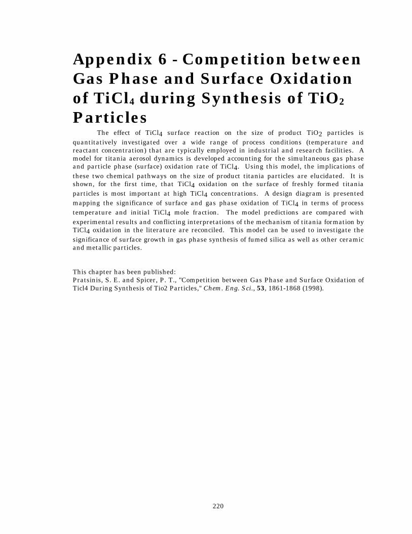
220

Appendix 6 - Competition between Gas Phase and Surface Oxidation of TiCl4 during Synthesis of TiO2 Particles

The effect of TiCl4 surface reaction on the size of product TiO2 particles is quantitatively investigated over a wide range of process conditions (temperature and reactant concentration) that are typically employed in industrial and research facilities. A model for titania aerosol dynamics is developed accounting for the simultaneous gas phase and particle phase (surface) oxidation rate of TiCl4. Using this model, the implications of these two chemical pathways on the size of product titania particles are elucidated. It is shown, for the first time, that TiCl4 oxidation on the surface of freshly formed titania particles is most important at high TiCl4 concentrations. A design diagram is presented mapping the significance of surface and gas phase oxidation of TiCl4 in terms of process temperature and initial TiCl4 mole fraction. The model predictions are compared with experimental results and conflicting interpretations of the mechanism of titania formation by TiCl4 oxidation in the literature are reconciled. This model can be used to investigate the significance of surface growth in gas phase synthesis of fumed silica as well as other ceramic and metallic particles. This chapter has been published: Pratsinis, S. E. and Spicer, P. T., "Competition between Gas Phase and Surface Oxidation of Ticl4 During Synthesis of Tio2 Particles," Chem. Eng. Sci., 53, 1861-1868 (1998).

221

Introduction Titania powders are made by TiCl4 oxidation in industrial flame aerosol reactors at high temperatures and moderate, near atmospheric, pressures by the so-called "chloride process" at a rate of 100 tons/day (Mezey, 1966; Stamatakis et al., 1991). This is a major process making more than half of the annual worldwide consumption of over 2 million tons of TiO2 aimed mostly for pigments and to a lesser extent as a paper filler, cosmetics, catalysts and even ceramic membranes. The fundamentals of this process are not yet well understood as chemical reaction and particle growth rapidly take place. As a result, it is hard to collect representative samples for particle sizing and eventual model development (Pratsinis, 1997). Even in the open literature, there are conflicting interpretations of TiO2 formation and growth by TiCl4 oxidation as a brief review will show shortly. This lack of understanding largely limits process development for manufacture of titania. This is a pity given the fact that this flame process has high potential for manufacture of a wide spectrum of ceramic powders (Pratsinis, 1997). George et al. (1973) systematically studied titania formation by TiCl4 oxidation in a premixed CO/O2 flame. They found that coagulation was dominant as the TiO2 size distributions were largely self-preserving while surface reactions were inadequate to quantitatively explain the particle growth rate. Nevertheless, Suyama et al. (1975, 1976) qualitatively proposed that nucleation and surface growth determined the primary particle size of titania made in hot-wall reactors. Morooka et al. (1989) showed that assuming rapid TiCl4 oxidation and coagulation overpredicted the particle size and proposed that particle growth took place largely by oxidation of TiCl4 on the particle surface. Akhtar et al. (1991), however, quantitatively showed that in their hot-wall reactor aggregate particles were formed by coagulation as they had a self-preserving size distribution. Hung and Katz (1992) studied titania formation in a counterflow diffusion flame reactor and postulated that particle formation took place by coagulation followed by surface growth and fusion as the particles encountered progressively higher temperatures during their flow out of the burner. More recently, Jang and Jeong (1995) found that preheating the reactants prior to their oxidation reaction decreases the particle size and slightly narrows the particle size distribution. They proposed that nucleation and surface oxidation dominated titania particle growth in their hot-wall reactor. Clearly there is a split in the current understanding of the fundamentals of titania particle formation and growth. This is attributed to a lack of a quantitative evaluation of the simultaneous gas phase and surface oxidation rates of TiCl4 on the characteristics of product TiO2. This paper presents such an evaluation using established reaction rates of the global overall oxidation rate of TiCl4 and its surface reaction. The growth of titania particles is simulated by a simple model of aerosol dynamics. The basics of TiO2 formation are elucidated and a diagram is presented in which process conditions for titania synthesis by surface or gas phase oxidation and coagulation are identified and compared to experimental data in the literature. This model can be used also in evaluating the significance of surface growth in a variety of processes involving aerosol syntheis of particles (e.g. fumed silica, alumina and metal particles from decomposition of precursor vapors).

Theory The overall oxidation reaction for TiCl4 is: TiCl4 + 2O2 -----> TiO2 + 2Cl2

222

and can be carried out in the gas phase or on a solid surface. Hence, two distinct chemical pathways for oxidation of TiCl4 vapor can be identified: First, vapor of TiCl4 may react with oxygen in the gas phase forming titania or precursor (oxychloride) particles at rate Rg. Second, TiCl4 vapor may react with oxygen on the surface of titania particles coating them with titania or precursor (oxychloride) films at rate Rs. As a result, the overall oxidation rate of TiCl4, R, can be written as (Pratsinis, 1997):

dCdt

R R Rg s= = + (8)

where C is the concentration of TiCl4 vapor (moles/cm3). Pratsinis et al. (1990) have measured R in the effective temperature range of 813 to 1173 K and TiCl4 mole fraction, φ =

5.6x10-4, or concentration of 2.5x10-8 moles/cm3:

R kC= − (9)

where:

k xT

=−

8 26 10

106814. exp (10)

and T is the temperature for TiCl4/O2 < 1/20. More recently, Kobata et al. (1991) have compiled a number of reaction rate data over a range of temperatures and reactant concentrations:

k xT

=−

25 10

122684 exp (11)

Ghoshtagore (1970) measured the growth rate of TiO2 films by surface reaction of TiCl4

between 673 and 1120 K and TiCl4 mole fraction of φ = 3.8x10-5 to 1.2x10-3:

R k ACs s= − (12) where:

k xTs =

−

4 9 10

89933. exp (13)

and A is the total aerosol surface area concentration (cm2/cm3) over which the TiCl4 oxidation takes place. This area may be constant during film growth while it is rapidly changing during powder manufacture since it is the area of the newly formed titania particles. To elucidate the role of these reaction rates, the concurrent dynamics of the titania aerosol need to be described and coupled to the kinetics through A. Though there are several models for particle growth at the above conditions, here the simplest possible one is chosen to explore the competition between TiCl4 gas and surface oxidation during synthesis of TiO2 aerosol neglecting the spread of its size distribution. Monodisperse models are quite attractive for description of aerosol dynamics involving concurrent gas phase chemistry and transport. For example, Warren and Seinfeld (1985) developed such a model that has been used in simulation of photochemical air pollution; Kim and Pratsinis (1989) developed another one that is used in simulation of manufacture of optical fiber preforms at AT&T while Panda and Pratsinis (1995) developed another one simulating synthesis of Al and Pd nanoparticles in a jet aerosol flow condenser (Haas et al., 1997). Of course, lognormal (Megaridis and Dobbins, 1990) and sectional (Gelbard et al., 1980) aerosol models provide more information on the dynamic behavior of the complete particle size distribution but they involve other assumptions, additional complexity and computational resources.

223

Nevertheless, monodisperse models can describe reasonably well integral properties of the particle size distribution such as the aerosol area, average size and number concentration (Landgrebe and Pratsinis, 1990; Kruis et al., 1993). Thus, neglecting the spread of the aerosol size distribution and assuming perfect coalescence upon particle collision, the rate of change of the total particle concentration N, (#/cm3), is given by (Panda and Pratsinis, 1995):

dNdt

IN

= −β 2

2 (14)

where β is the collision frequency function of equally sized particles from free molecule to continuum particle size regime (Fuchs, 1964; Phillips, 1972; Seinfeld, 1986). The nucleation rate I (#/cm3/s) is equal to the rate of new particle (here, molecule) formation by gas phase chemical reaction over a wide range of conditions (Ulrich, 1971; George et al., 1973; Xiong and Pratsinis, 1991): I R Ng A= − (15)

and NA is the Avogadro number. It should be emphasized that this is a simplified representation of the actual process for lack of reliable information on the early stages of TiO2 formation (Pratsinis et al., 1990). Clearly, the first right hand side (RHS) term of (14) represents the addition of new particles by nucleation while the second RHS term stands for the loss of particles by coagulation. Similarly, the rate of change of the total titania aerosol volume V (cm3/cm3) is: dVdt

Iv R N vs A= +1 1 (16)

where v1 is the volume of a TiO2 molecule in solid state (ρp = 4 g/cm3). The first RHS term of (16) accounts for the formation of titania aerosol volume by nucleation while the second RHS term accounts for the formation of titania aerosol by surface reaction. The average particle diameter, dp, is

dVNp=

61

3

π (17)

while the total aerosol surface area concentration (cm2/cm3) is

A N dp= π 2 (18)

The above set of equations describes the overall TiCl4 kinetics and TiO2 aerosol dynamics at isothermal conditions. These conditions are used to clearly demonstrate the competition of the two reaction pathways at various temperature levels. The above set of equations was solved using the DGEAR routine (IMSL,1980; Spicer, 1997).


Selection of Simulation Conditions Titania is made by the "chloride" process by supplying TiCl4 and oxygen at almost stoichiometric conditions (corresponding to TiCl4 mole fraction, φ, near 0.5) in flame reactors operating at near atmospheric pressure and T= 1000 - 1500 C at very short residence times (e.g. Nelson et al., 1963). On the other hand, typical conditions in research laboratories involve similar temperatures and pressures but longer residence times and lower TiCl4 concentrations (Table 1). As a result, here, the significance of gas phase or surface oxidation

224

of TiCl4 on the diameter of product TiO2 is investigated at atmospheric pressure, T = 1000-1800 K and φ = 0.0001-0.5 in oxygen carrier gas as in most laboratory studies. The overall oxidation rate of TiCl4 was described using the rate of Pratsinis et al. (1990). The expression of Kobata et al. (1991) overpredicted the TiCl4 conversion by 10% and the TiO2 diameter by less than 1% at 1000K while the predictions of the model by Kobata et al. (1990) were indistinguishable from those of the model of Pratsinis et al. (1990) at 1400 K. The use of oxygen instead of chlorine as carrier gas, as it would be appropriate for simulation titania growth at highly concentrated synthesis conditions, did not alter the model results more than 1%. Finally, this model can be easily adopted to describe titania formation by TiCl4 oxidation in the absence of surface reaction by merely setting ks = 0 reducing it to that of Landgrebe and Pratsinis (1990).

TiO2 Formation and Growth by Surface and Gas Phase Oxidation of TiCl4 Figure 1 shows the evolution of a) the average particle diameter, dp, and b) the total particle number concentration, N, and aerosol surface area, A, accounting for surface reaction (solid lines) and neglecting it (broken lines, ks = 0) at 1000 K and TiCl4 mole

fraction φ = 0.01 at 1 atm from t = 10-4 to 100 s. Figure 1a also shows the corresponding overall conversion, C/C0, of TiCl4 (dotted line) at 1000 K. Particle growth starts from about 4 nm corresponding to the molecular size of titania (Figure 1a). When the surface reaction is neglected, the particle number concentration increases at t<10-3s (Figure 1b, broken lines) as new particles (molecules) are formed by chemical reaction. As the number of particles increases, coagulation becomes important and the chemical reaction cannot make up the loss of particles by coagulation so N starts to slowly decrease up to t = 1s. At that time about 90% of TiCl4 has been consumed (Figure 1a) and the addition of new particles by pure gas phase reaction slows down so coagulation completely takes over, decreasing N steeply at t>1s. The aerosol area increases rapidly at first (t<10-3s) as addition of new particles by reaction is dominant (Figure 1b). Later on, as coagulation becomes important, A continues to increase but at a slower rate until it reaches a maximum at t = 1s when the contribution of chemical reaction is no longer significant. At t>1s the aerosol area decreases by coagulation. When surface reaction is taken into account (Figure 1, solid lines), newly formed particles have considerable surface area at t>0.001s. Then, TiCl4 oxidation on the particle surface competes effectively with gas phase oxidation of TiCl4 reducing the nucleation (or formation) rate of new particles. As a result, particle losses by coagulation cannot be made up by nucleation (or gas phase reaction) and the total particle concentration decreases faster than when surface reaction was neglected. This continues until t~1s when the reduction in N seems to nearly level off at t~5s. During this period, N has been decreasing so much that the contribution by pure gas phase oxidation can almost balance the reduction by coagulation. Of course, as the TiCl4 concentration decreases (Figure 1a), the contribution by gas phase oxidation becomes insignificant so N decreases again steeply, converging to the evolution of N in the absence of surface reaction (t>5s). Figure 1a shows that particle size increases much faster by surface than by gas phase oxidation and coagulation (t = 0.01-1 s) while the aerosol area remains nearly constant by the balance of surface growth and coagulation in the free molecule size regime up to t~5s (Figure 1b). It is worth pointing out that the area of atmospheric aerosols growing by surface reactions and coagulation in the free molecule regime remains constant as was measured by Husar and Whitby (1973) and annotated by Friedlander (1977: p. 274). In production

225

aerosols, reactions last as long as reactants are available and here this is the case at about 5 seconds (while atmospheric reactions last much longer). Then, the area is no longer constant and decreases by coagulation as discussed above. It is worth highlighting the difference surface reaction makes on particle size: At t = 1s the diameter of particles grown by surface and gas phase reaction is 60 nm while in the absence of surface reaction dp is only 10 nm. At longer residence times (t>5s), when there is no more TiCl4, coagulation dominates particle growth and the two models converge.

Effect of TiCl4 Mole Fraction, φ, and T on Titania Diameter Figure 2 shows the evolution of the particle diameter from t = 10-4 to 100 s for initial TiCl4 mole fraction φ = 0.001 and 0.1 at 1000 K accounting for the surface reaction (solid lines) and neglecting it (broken lines). At low TiCl4 concentrations (φ<0.001), accounting for the surface reaction little affects the evolution of particle size. Clearly, gas phase reaction and coagulation dominate particle formation and growth at this and lower TiCl4 mole fractions at all residence times. For larger φ, higher TiCl4 concentrations (φ = 0.1) increase the significance of surface reaction as the abundance of available surface area of freshly formed TiO2 participates and catalyzes the oxidation of TiCl4. Thus, at 1s residence time, the average titania particle diameter accounting for surface reaction is 300 nm while neglecting it, gives dp of only 15 nm. Of course, at very long residence times the predictions of the two models converge since again coagulation dominates and TiCl4 has been fully converted. However, this may be a rather misleading assurance because this model neglects the finite coalescence (sintering) rate of titania. As a matter of fact, at these low temperatures the sintering rate of titania is rather slow, so colliding particles will not grow to single coalesced ones but will form aggregates of fine primary particles. Figure 3 shows the evolution of titania particle diameter at T = 1400K at φ = 0.1 and 0.001 up to 100 seconds residence time. It should be noted that this temperature is outside the regime over which the overall and surface reaction rates have been measured so these results should be viewed with caution. Nevertheless, these reaction rates are routinely used at higher temperatures as is the case for SiCl4 oxidation in manufacture of optical fibers (Powers et al., 1978). Again, at intermediate residence times, accounting for surface reaction results in much larger particles than when it is neglected. A difference between 1000 K and 1400 K is that the dominance of surface reaction occurs earlier on following faster conversion of TiCl4. These results point out that accounting for oxidation of TiCl4 on the surface of newly formed titania particles substantially accelerates their growth. For example, at φ = 0.1 it is clear that particles experience rapid growth up to 0.1 s by surface reaction while after that they grow rather sluggishly by coagulation. This is hardly surprising because dp~t during

surface growth while during coagulation dp~t2/5 in the free molecule regime or dp~t1/3 in the continuum regime (Friedlander, 1977). This also shows that accounting for surface oxidation of TiCl4, results in particle growth up to dp = 0.2 µm within 0.1 s when more than 98% of TiCl4 has been consumed at 1400 K and φ = 0.1. Prolonging the residence time increases the size by coagulation (which widens the size distribution) and, possibly, the extent of aggregation because sintering and coalescence may determine the structure of coagulating particles at this temperature and residence time. Before concluding this section the significance of the assumption of rapid coalescence must be discussed. Neglecting coalescence, underpredicts the aerosol area since agglomerates have larger area than equivalent spheres. This assumption will be most

226

important at short residence times, large dp and low T especially when coagulation dominates particle growth. These two assumptions may partially compensate for each other. A detailed evaluation of these assumptions can be done with models accounting for the detailed size and structure distribution of agglomerate particles (Xiong and Pratsinis, 1993).

Criteria for TiO2 Synthesis by Coagulation or Surface Growth The above results indicate that at high initial TiCl4 mole fractions (e.g. φ>0.001) surface growth may significantly affect the size of product TiO2 particles. Thus, pure gas phase reaction is responsible for the early formation of titania particles. These particles may have large enough surface area to catalyze TiCl4 oxidation on their surface and prevent significant formation of new TiO2 particles by pure gas phase reaction. Since fewer particles are present, they are growing larger by surface reaction rather than by gas phase reaction and coagulation. Of course at long residence times when virtually all TiCl4 has been converted to TiO2, coagulation again determines the particle growth rate. At very long residence times the mechanism of TiO2 formation may have little effect on particle size . However, typical residence times are not that long, especially, taking into account that sintering affects the coalescence rate of colliding particles. Hence it may be significant to know process conditions that favor particle growth by surface oxidation rather than by pure gas phase oxidation. Typically, it is required to produce titania of a specific size, among other characteristics, depending on the final application. It would be of interest to select process conditions that favor surface growth during production of titania of that size. Figure 4 shows a diagram of the initial TiCl4 mole fraction, φ, and product TiO2 diameter, dp, in which particle growth is dominated either by surface oxidation or gas phase oxidation of TiCl4 at various T. Each boundary is the isopleth of particle diameters in which the model that accounts for surface oxidation predicts a particle diameter 5% larger than that of the model that neglects surface reaction (squares in Figure 1a). For example, during an actual process at isothermal conditions, gas phase reaction and coagulation (or nucleation) dominates at the early stages of the process and consequently at very small particle sizes (left region outside of the U shaped curves). Later on and for φ>0.0005, surface reaction dominates (middle region). For long residence times, coagulation again becomes important (right region). Figure 4 shows that surface reaction affects titania growth at high TiCl4 mole fractions (φ>0.001) for synthesis of particles in the range of 50-1000 nm. Outside this region, coagulation dominates and the resulting particles may have broad size distributions as dictated by the self-preserving theory. The most fascinating result of this study, however, is the identification of the surface growth region of the diagram (inside the U shaped curves for each T). There, particles of narrow size distribution with limited extent of agglomeration can be made. Though the present model does not describe the dynamics of the particle size distribution, Pratsinis (1988) has shown that when coagulation and condensation simultaneously take place, the resulting particles have size distribution narrower than that dictated by the self-preserving theory (Friedlander, 1977). Since growth by surface reaction is equivalent to growth by condensation in the free molecule regime, we should expect relatively narrower size distributions for the particles made in the surface growth region rather than in the pure gas phase reaction region. For synthesis of non-aggregate powders such as desired in pigments and cosmetics, one should operate in this region. However, if aggregate particles with high specific surface area are desired such as in photocatalysis and catalysis, in general, surface growth should be minimized and particles should be made outside this region.

227

Comparison with Experimental Results Figure 4 shows also the conditions at which titania powders were made by various investigators. Table 1 lists the range of average size of titania powders made by these researchers and the corresponding range of φ and T. For example, George et al. (1973) who reported that surface growth was not important in their experiments, had operated at φ = 10-5 to 10-3 up to 1650K. Their conditions confined them well outside the surface growth region of this process as Figure 4 shows. Likewise, Akhtar et al. (1991) who produced titania at φ = 0.0002-0.001 had operated just outside the surface growth region and coagulation determined particle growth at their conditions. Suyama et al. (1975 and 1976) who claimed nucleation and surface growth as the mechanism for titania particle formation operated at high TiCl4 volume fractions, φ = 0.006-0.11 as well as Morooka et al. (1989), φ = 0.003-0.014 are in excellent agreement with Figure 4. Hung and Katz (1992) operated at φ = 0.0002 and were outside the surface growth region for early stage particle formation so Figure 4 is in agreement even with their speculation. The majority of the data by Jang and Jeong (1995) belong to the surface growth region of Figure 4 in agreement with their assessment that nucleation and surface growth dominated titania formation. As a matter of fact, all their primary particle size distributions have geometric standard deviations below the self-preserving limit (σg = 1.45) that slightly decrease as φ increases in agreement with the expectation of narrower size distributions with increased dominance of surface reaction (Pratsinis, 1988).

Conclusions During synthesis of titania powders by TiCl4 oxidation at high temperatures, the

initial mole fraction of TiCl4, φ, largely determines the significance of pure gas phase or surface oxidation. Simply put, high TiCl4 concentrations result in high concentrations of TiO2 nuclei that have enough surface area to consume TiCl4 by surface reaction and effectively quench pure gas phase oxidation of TiCl4. At the other extreme, low TiCl4 concentrations produce low concentrations of TiO2 nuclei that never have enough area for surface reaction to compete with pure gas phase reaction. As a result, nuclei are continuously formed at high enough concentrations and grow by coagulation. A model was developed for this process elucidating these phenomena using literature expressions for the reaction rates and accounting for the titania aerosol dynamics neglecting the spread of the distribution and the coalescence rate of titania at isothermal conditions. This model quantitatively defined the regions of dominance of gas and surface oxidation of TiCl4 at various process temperatures. Furthermore, it explained and reconciled apparent conflicts in the literature regarding the fundamentals of titania formation and growth by TiCl4 oxidation. It is particularly significant the discovery of specific process conditions where surface growth is dominant indicating the possibility for synthesis of particles with narrow size distributions. Even a small reduction (say 10%) in the polydispersity of the product may have significant impact in this industry given its huge product volumes, more than a million tons per year. The results of this simple model should not be surprising as surface growth is dominant in flame synthesis of carbon blacks which is similar to flame synthesis of titania by TiCl4 oxidation. Likewise there is a strong likelihood that surface growth can be important in aerosol synthesis of fumed silica, lightguide preforms, and other ceramic and metallic

228

powders and nanoparticles that are made by gas phase reaction (oxidation or thermal decomposition) of precursor vapors. This model can be used for a quick evaluation of the significance of surface growth provided that the required chemical data are available. Furthermore, models that explicitly account for simultaneous chemical reactions including gas phase and surface growth, coagulation and sintering of polydisperse aerosols will further contribute to revealing of conditions for synthesis of monodisperse titania and other, even nanosize powders.

Acknowledgments We acknowledge support by the National Science Foundation, CTS-9619392 and

stimulating discussions with Dr. Srinivas Vemury (Lucent Technologies Inc.) and Dr. Roger Place (International Fine Particle Research Institute).

229

References Akhtar, M. K., Y. Xiong and S. E. Pratsinis, “Vapor Synthesis of Titania Powder by Titanium

Tetrachloride Oxidation,” AIChE J., 37, 1561-1570 (1991). Akhtar, M.K., S.E. Pratsinis, S.V.R. Mastrangelo, "Dopants in Vapor Phase Synthesis of

Titania Powders", J. Amer. Ceram. Soc., 75, 3408-3416 (1992). Friedlander, S. K. 1977. Smoke, Dust and Haze. New York : John Wiley and Sons. Fuchs, N. A., The Mechanics of Aerosols, Pergamon Press, Elmsford, NY, 1964. Gelbard, F., Tambour, Y. and Seinfeld, J.H. (1980). “Sectional representations for simulating

aerosol dynamics,” J. Colloid Interface Sci., 76, 541-556 George, A.P., R.D. Murley, E.R. Place, "Formation of TiO2 aerosol from the Combustion

Supported Reaction of TiCl4 and O2", Symp. Farad. Soc., 7 63-71(1973). Ghoshtagore R.N., "Mechanism of Heterogeneous Deposition of Thin film rutile", J.

Electrochem. Soc. Solid State Sci , 117, 529-534(1970) Haas, V., R. Birringer, H. Gleiter, S.E. Pratsinis, "Synthesis of Nanostructured Powders in

an Aerosol Flow Condenser", J. Aerosol Sci. in press (1997). Hung, C. -H. and Katz, J. L., "Formation of mixed oxide powders in flames: Part I. TiO2-

SiO2", J. Mater. Res., 7, 1861-1869 (1992). Husar, R.B. and K.T. Whitby, "Growth Mechanisms and Size Spectra of Photochemical

Aerosols", Environ. Sci. Technol., 7, 241-7(1973). IMSL, IMSL Contents Document, 8th ed. International Mathematical and Statistical

Libraries, Houston (1980). Jang, H.-D., J. Jeong, "The Effects of Temperature on Particle Size in the Gas Phase

Production of TiO2",Aerosol Sci. Technol. 23, 553-60 (1995). Kim K.S., S.E. Pratsinis, "Modeling and Analysis of Modified Chemical Vapor Deposition of

Optical Fiber Preforms", Chem. Eng. Sci., 44, 2475-2482 (1989). Kobata A., K. Kusakabe and S. Morooka, "Growth and Transformation of TiO2 Crystallites

in Aerosol Reactor", AIChE J., 37, 347-59 (1991). Kruis F.E., K. Kusters, S.E. Pratsinis, B. Scarlett, "A Simple Model for the Evolution of the

Characteristics of Aggregate Particles undergoing Coagulation and Sintering" Aerosol Sci. Technol. 19, 514-526 (1993).

Landgrebe, J.D. and Pratsinis, S.E. (1990). “A Discrete-Sectional Model for Particulate Production by Gas-Phase Chemical Reaction and Aerosol Coagulation in the Free-Molecular Regime,” J. Coll. Interface Sci., 139, 63-85

Megaridis C.M. and R.A. Dobbins, "A Bimodal Integral Solution of the Dynamic Equation for an Aerosol Undergoing Simultaneous Particle Inception and Coagulation", Aerosol Sci. Technol. 12, 240-55 (1990).

Mezey, E. J., "Pigments and Reinforcing Agents," in Vapor Deposition , C. F. Powell, J. H. Oxley and J. M. Blocher, Jr., eds., John Wiley & Sons, New York, 423-451 (1966).

Morooka, S., T. Yasutake, A. Kobata, K. Ikemizu, Y. Kato, "A Mechanism for the Production of Ultrafine Particles of TiO2 by a Gas Phase Reaction", Int. Chem. Eng., 29, 119-26(1989).

Nelson, E.W., J.E. Bondurant, J.P. Wikswo G.C. Marcot, "Manufacture of Titanium Dioxide Pigment", Brit. Patent 916,250 (1963).

Panda S., S.E. Pratsinis "Modeling the Synthesis of Aluminum Particles by Evaporation-Condensation in an Aerosol Flow Reactor", Nanostructured Mater. 5, 755-68 (1995).

Powers, D.R. “Kinetics of SiCl4, Oxidation” J. Am. Ceram. Soc.., 61, 295-7 (1978). Pratsinis, S.E., "Flame Aerosol Synthesis of Ceramic Powders" Prog. Energy Combust. Sci. in

press (1997). Pratsinis, S. E., H. Bai, P. Biswas, M. Frenklach and S. V. R. Mastrangelo, “Kinetics of TiCl4

Oxidation”, J. Am. Ceram. Soc., 73, 2158-2162 (1990).

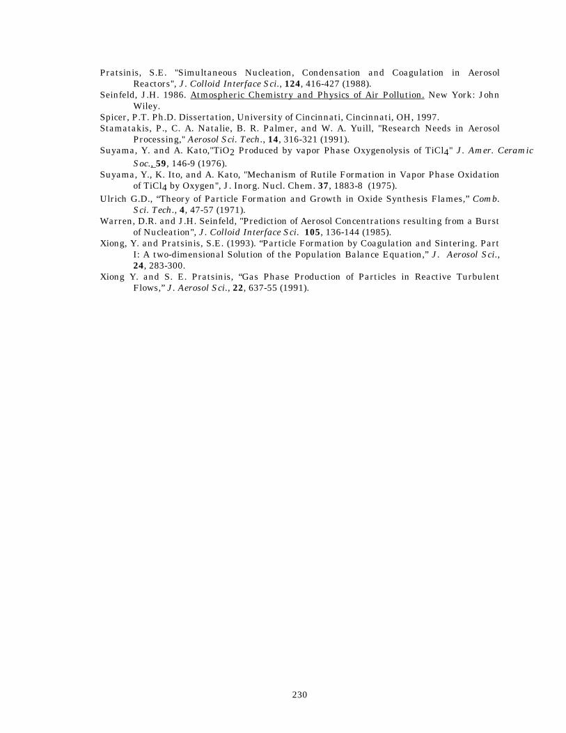
230

Pratsinis, S.E. "Simultaneous Nucleation, Condensation and Coagulation in Aerosol Reactors", J. Colloid Interface Sci., 124, 416-427 (1988).

Seinfeld, J.H. 1986. Atmospheric Chemistry and Physics of Air Pollution. New York: John Wiley.

Spicer, P.T. Ph.D. Dissertation, University of Cincinnati, Cincinnati, OH, 1997. Stamatakis, P., C. A. Natalie, B. R. Palmer, and W. A. Yuill, "Research Needs in Aerosol

Processing," Aerosol Sci. Tech., 14, 316-321 (1991). Suyama, Y. and A. Kato,"TiO2 Produced by vapor Phase Oxygenolysis of TiCl4" J. Amer. Ceramic

Soc., 59, 146-9 (1976). Suyama, Y., K. Ito, and A. Kato, "Mechanism of Rutile Formation in Vapor Phase Oxidation

of TiCl4 by Oxygen", J. Inorg. Nucl. Chem. 37, 1883-8 (1975). Ulrich G.D., “Theory of Particle Formation and Growth in Oxide Synthesis Flames,” Comb.

Sci. Tech., 4, 47-57 (1971). Warren, D.R. and J.H. Seinfeld, "Prediction of Aerosol Concentrations resulting from a Burst

of Nucleation", J. Colloid Interface Sci. 105, 136-144 (1985). Xiong, Y. and Pratsinis, S.E. (1993). “Particle Formation by Coagulation and Sintering. Part

I: A two-dimensional Solution of the Population Balance Equation,” J. Aerosol Sci., 24, 283-300.

Xiong Y. and S. E. Pratsinis, “Gas Phase Production of Particles in Reactive Turbulent Flows,” J. Aerosol Sci., 22, 637-55 (1991).

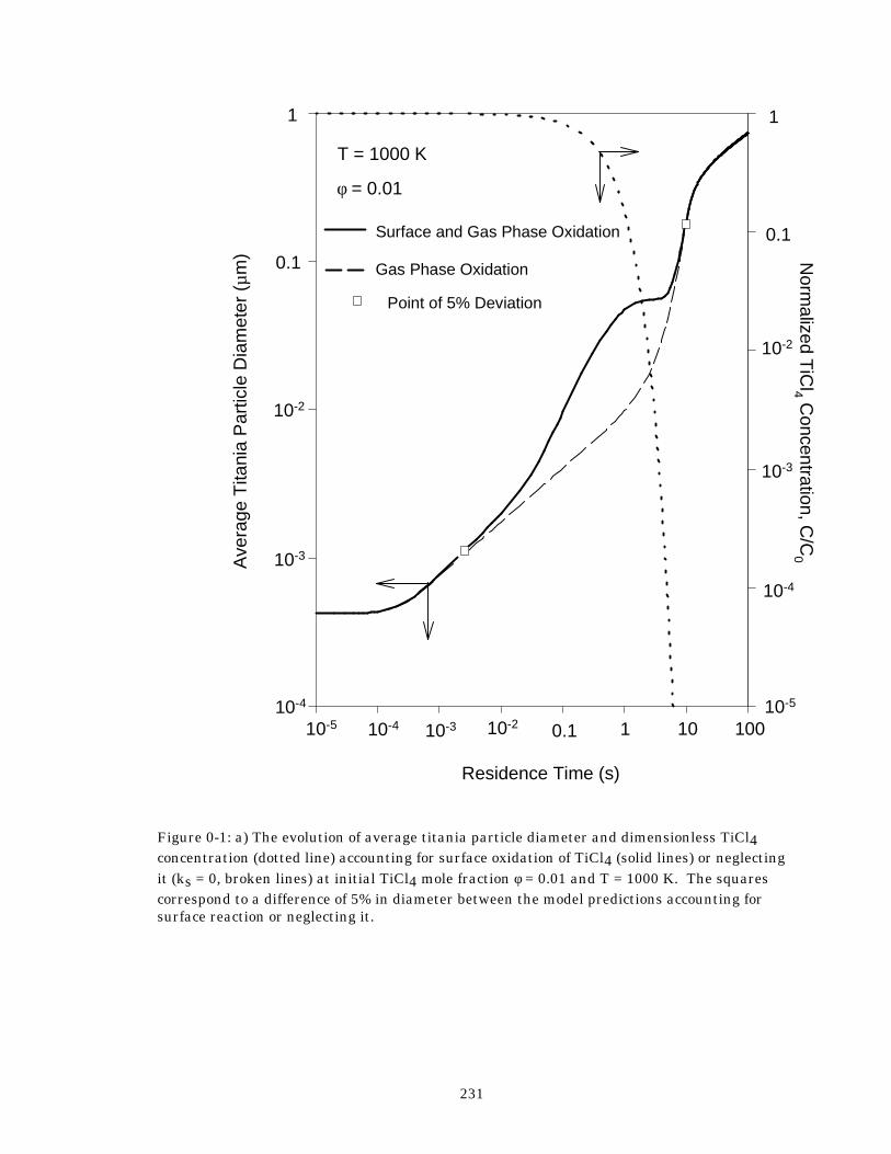
231

Figure 0-1: a) The evolution of average titania particle diameter and dimensionless TiCl4 concentration (dotted line) accounting for surface oxidation of TiCl4 (solid lines) or neglecting it (ks = 0, broken lines) at initial TiCl4 mole fraction φ = 0.01 and T = 1000 K. The squares correspond to a difference of 5% in diameter between the model predictions accounting for surface reaction or neglecting it.

Residence Time (s)

Ave

rage

Tita

nia

Par

ticle

Dia

met

er (µ

m) N

ormalized T

iCl4 C

oncentration, C/C

0

Surface and Gas Phase Oxidation

Gas Phase Oxidation

T = 1000 K

φ = 0.01

1

0.1

10-2

10-3

10-4

110-210-310-4 0.1 1010-5

1

10-2

10-3

10-4

0.1

10-5

Point of 5% Deviation

100

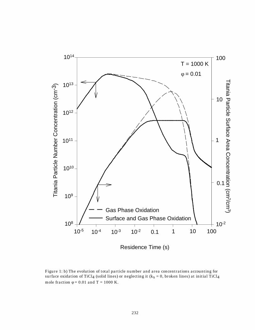
232

Figure 1: b) The evolution of total particle number and area concentrations accounting for surface oxidation of TiCl4 (solid lines) or neglecting it (ks = 0, broken lines) at initial TiCl4 mole fraction φ = 0.01 and T = 1000 K.

Residence Time (s)

Tita

nia

Par

ticle

Num

ber

Con

cent

ratio

n (c

m-3

)

Titania P

article Surface A

rea Concentration (cm

2/cm3)

110-210-310-4 0.1 1010-5

T = 1000 K

φ = 0.01

Surface and Gas Phase OxidationGas Phase Oxidation

100

10-2

10

1

0.1

109

108

1010

1012

1011

1013

1014

100

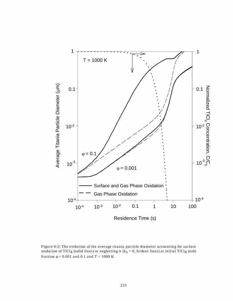
233

Figure 0-2: The evolution of the average titania particle diameter accounting for surface oxidation of TiCl4 (solid lines) or neglecting it (ks = 0, broken lines) at initial TiCl4 mole fraction φ = 0.001 and 0.1 and T = 1000 K.

Residence Time (s)

Ave

rage

Tita

nia

Par

ticle

Dia

met

er (

µm) N

ormalized T

iCl4 C

oncentration, C/C

0

T = 1000 K

φ = 0.001

Gas Phase Oxidation


φ = 0.1

1

0.1

10-2

10-3

10-4

10-4 1010.110-210-3

1

0.1

10-2

10-3

10-4

100

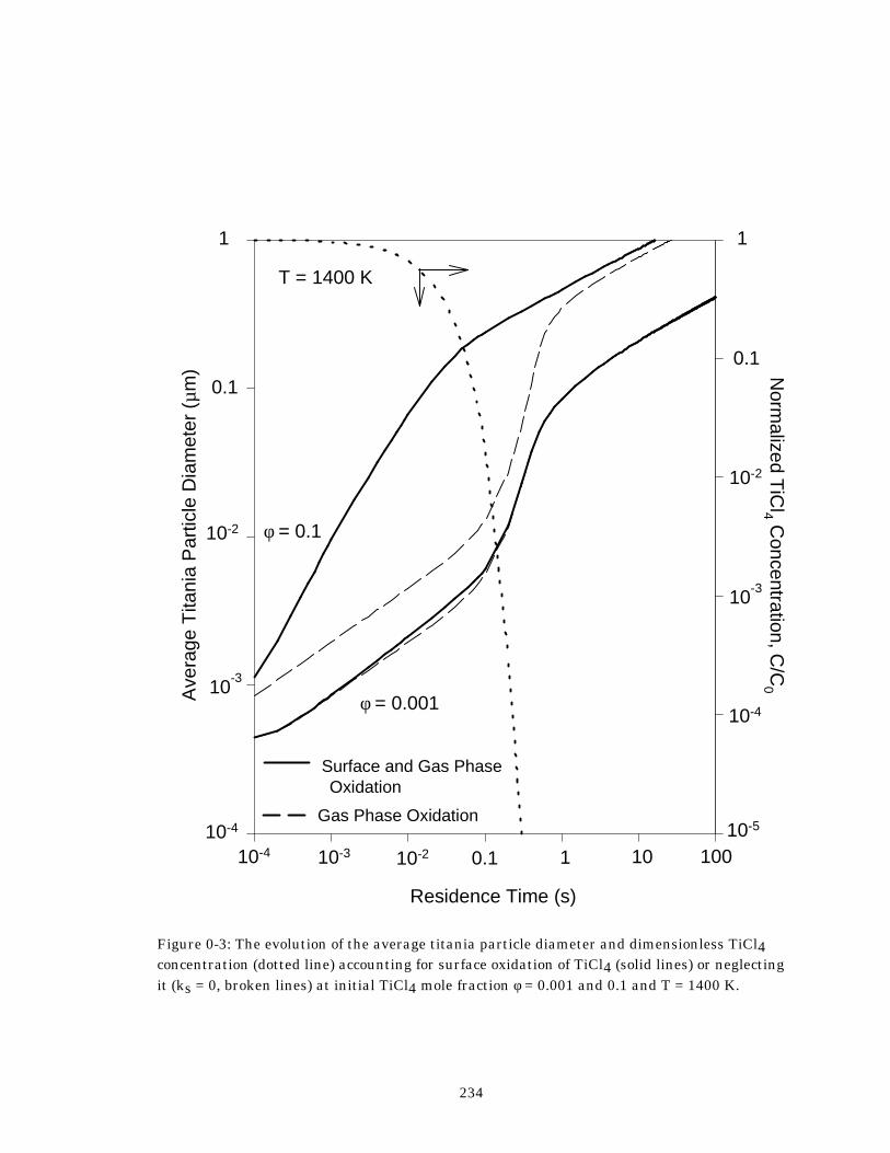
234

Figure 0-3: The evolution of the average titania particle diameter and dimensionless TiCl4 concentration (dotted line) accounting for surface oxidation of TiCl4 (solid lines) or neglecting it (ks = 0, broken lines) at initial TiCl4 mole fraction φ = 0.001 and 0.1 and T = 1400 K.

Residence Time (s)

Ave

rage

Tita

nia

Par

ticle

Dia

met

er (

µm) N

ormalized T

iCl4 C

oncentration, C/C

0

T = 1400 K

φ = 0.1

10-4 1010.110-210-3

φ = 0.001

1

0.1

10-2

10-3

10-4

10-5

1

0.1

10-2

10-3

10-4

100

Gas Phase Oxidation

Surface and Gas PhaseOxidation

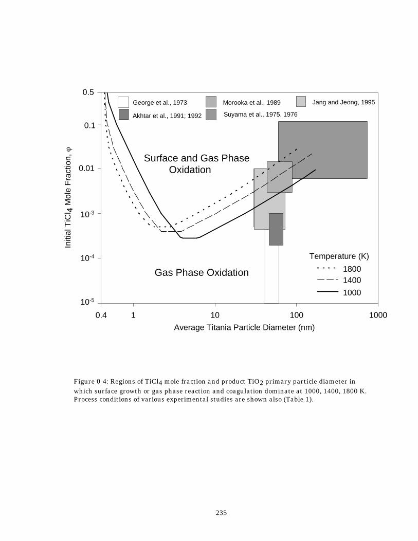
235

Figure 0-4: Regions of TiCl4 mole fraction and product TiO2 primary particle diameter in which surface growth or gas phase reaction and coagulation dominate at 1000, 1400, 1800 K. Process conditions of various experimental studies are shown also (Table 1).

Average Titania Particle Diameter (nm)1 10 100 1000

Initi

al T

iCl 4

Mol

e F

ract

ion,

φ

0.1

0.01

10-3

10-4

0.5

0.4

Suyama et al., 1975, 1976

Morooka et al., 1989 Jang and Jeong, 1995

Gas Phase Oxidation


10-5

George et al., 1973

Akhtar et al., 1991; 1992

Temperature (K)

1000

14001800

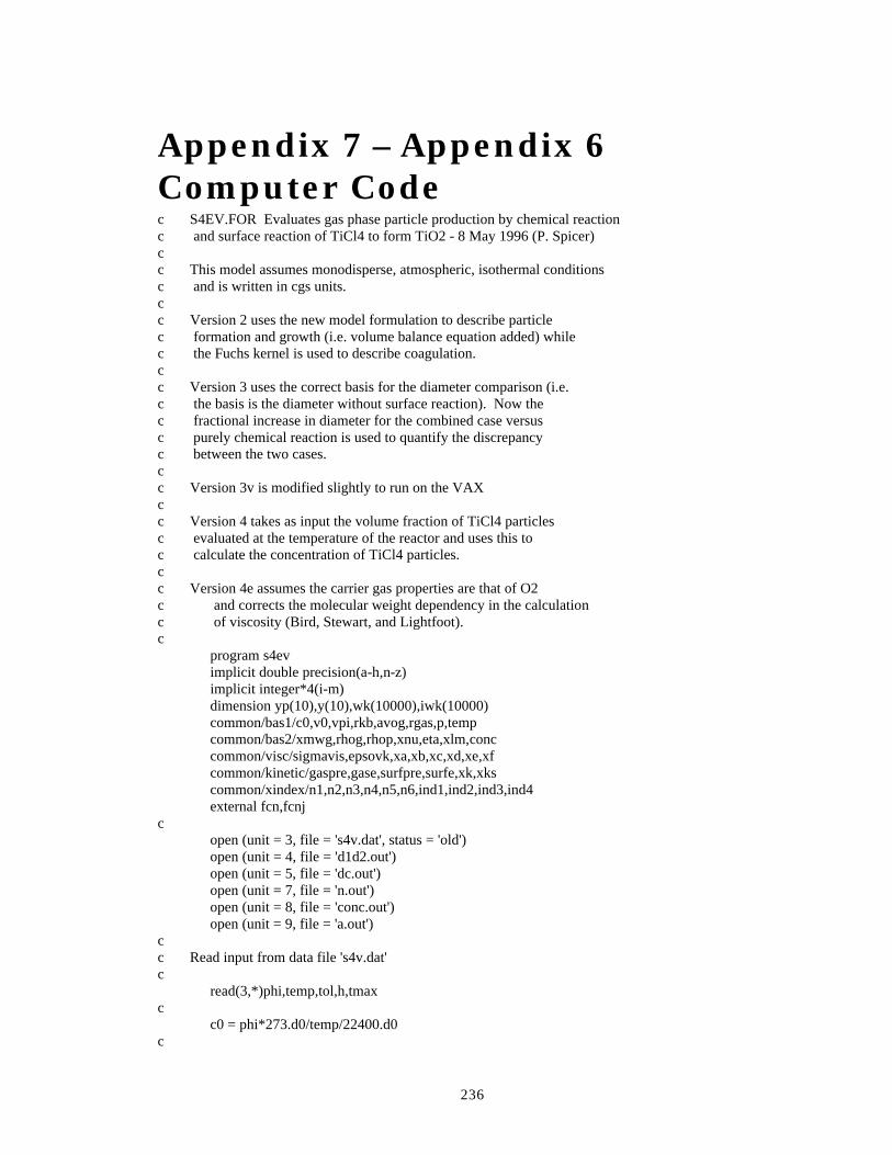
236

Appendix 7 – Appendix 6 Computer Code c S4EV.FOR Evaluates gas phase particle production by chemical reaction c and surface reaction of TiCl4 to form TiO2 - 8 May 1996 (P. Spicer) c c This model assumes monodisperse, atmospheric, isothermal conditions c and is written in cgs units. c c Version 2 uses the new model formulation to describe particle c formation and growth (i.e. volume balance equation added) while c the Fuchs kernel is used to describe coagulation. c c Version 3 uses the correct basis for the diameter comparison (i.e. c the basis is the diameter without surface reaction). Now the c fractional increase in diameter for the combined case versus c purely chemical reaction is used to quantify the discrepancy c between the two cases. c c Version 3v is modified slightly to run on the VAX c c Version 4 takes as input the volume fraction of TiCl4 particles c evaluated at the temperature of the reactor and uses this to c calculate the concentration of TiCl4 particles. c c Version 4e assumes the carrier gas properties are that of O2 c and corrects the molecular weight dependency in the calculation c of viscosity (Bird, Stewart, and Lightfoot). c program s4ev implicit double precision(a-h,n-z) implicit integer*4(i-m) dimension yp(10),y(10),wk(10000),iwk(10000) common/bas1/c0,v0,vpi,rkb,avog,rgas,p,temp common/bas2/xmwg,rhog,rhop,xnu,eta,xlm,conc common/visc/sigmavis,epsovk,xa,xb,xc,xd,xe,xf common/kinetic/gaspre,gase,surfpre,surfe,xk,xks common/xindex/n1,n2,n3,n4,n5,n6,ind1,ind2,ind3,ind4 external fcn,fcnj c open (unit = 3, file = 's4v.dat', status = 'old') open (unit = 4, file = 'd1d2.out') open (unit = 5, file = 'dc.out') open (unit = 7, file = 'n.out') open (unit = 8, file = 'conc.out') open (unit = 9, file = 'a.out') c c Read input from data file 's4v.dat' c read(3,*)phi,temp,tol,h,tmax c c0 = phi*273.d0/temp/22400.d0 c

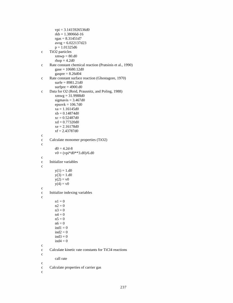
237

vpi = 3.1415926536d0 rkb = 1.38066d-16 rgas = 8.31451d7 avog = 6.022137d23 p = 1.01325d6 c TiO2 particles xmwp = 80.d0 rhop = 4.2d0 c Rate constant chemical reaction (Pratsinis et al., 1990) gase = 10680.12d0 gaspre = 8.26d04 c Rate constant surface reaction (Ghostagore, 1970) surfe = 8981.21d0 surfpre = 4900.d0 c Data for O2 (Reid, Prausnitz, and Poling, 1988) xmwg = 31.9988d0 sigmavis = 3.467d0 epsovk = 106.7d0 xa = 1.16145d0 xb = 0.14874d0 xc = 0.52487d0 xd = 0.77320d0 xe = 2.16178d0 xf = 2.43787d0 c c Calculate monomer properties (TiO2) c d0 = 4.2d-8 v0 = (vpi*d0**3.d0)/6.d0 c c Initialize variables c y(1) = 1.d0 y(3) = 1.d0 y(2) = v0 y(4) = v0 c c Initialize indexing variables c n1 = 0 n2 = 0 n3 = 0 n4 = 0 n5 = 0 n6 = 0 ind1 = 0 ind2 = 0 ind3 = 0 ind4 = 0 c c Calculate kinetic rate constants for TiCl4 reactions c call rate c c Calculate properties of carrier gas c

238

call props c c Dgear Parameters c imeth = 2 imiter = 1 index = 1 ier = 0 t = 0.d0 max = 4 c c%%%%%%%%%%%%%%%%%%%%%%%%%%%%%%%%%%%%%%%%%%%%%%%%%%%%%%%%%%%%%%%%%%%%%%%% c Call Dgear Solver Routine c 100 if (t.lt.1.d-4) then tend = t + 1.d-5 elseif (t.lt.1.d-3) then tend = t + 1.d-4 elseif (t.lt.1.d-2.and.t.ge.1.d-3) then tend = t + 1.d-3 elseif (t.lt.1.d-1.and.t.ge.1.d-2) then tend = t + 1.d-2 elseif (t.lt.1.d0.and.t.ge.1.d-1) then tend = t + 1.d-1 elseif (t.lt.tmax.and.t.ge.1.d0) then tend = t + 0.5d0 endif c call dgear(max,fcn,fcnj,t,h,y,tend,tol,imeth, 2 imiter,index,iwk,wk,ier) c c if (ier.gt.128) then c write(6,*)'Error = ',ier c go to 10 c endif c call diam(y,d1,d2) write(4,175)t,d1*1.d4,d2*1.d4 write(7,180)t,y(1),y(3) write(8,185)t,conc/c0 write(9,190)t,vpi*d1*d1*y(1),vpi*d2*d2*y(3) c if (t.lt.tmax) go to 100 c%%%%%%%%%%%%%%%%%%%%%%%%%%%%%%%%%%%%%%%%%%%%%%%%%%%%%%%%%%%%%%%%%%%%%%%%% c c Output run conditions at end of each output file c do 150 i = 4,5 write(i,200)temp,phi,c0 150 continue 175 format(3(1x,e12.6)) 180 format(3(1x,e12.6)) 185 format(2(1x,e12.6)) 190 format(3(1x,e12.6))

239

200 format(3(1x,e12.6)) c 10 stop end c c c------------------------SUBROUTINES---------------------------------- c c c************************************************************************ c Differential Equations to be solved c************************************************************************ subroutine fcn(max,t,y,yp) implicit double precision(a-h,n-z) implicit integer*4(i-m) common/bas1/c0,v0,vpi,rkb,avog,rgas,p,temp common/bas2/xmwg,rhog,rhop,xnu,eta,xlm,conc common/kinetic/gaspre,gase,surfpre,surfe,xk,xks dimension y(10),yp(10) external fuchs,diam c conc = c0*exp(-xk*t) c if (conc.lt.0.d0) then conc = 0.d0 write(6,*)'< 0' endif c call diam(y,d1,d2) c call fuchs(d1,beta1) call fuchs(d2,beta2) c c Case with surface reaction c xi = xk - xks*vpi*d1*d1*y(1) if(xi.le.0.d0) then xi = 0.d0 endif c yp(1) = xi*conc*avog - 0.5d0*beta1*y(1)*y(1) yp(2) = (xi + xks*vpi*d1*d1*y(1))*conc*avog*v0 c c Case without surface reaction c yp(3) = xk*conc*avog - 0.5d0*beta2*y(3)*y(3) yp(4) = xk*conc*avog*v0 c return end c********************************************************************** c Calculate and compare average diameters from each calculation c********************************************************************** subroutine diam(y,d1,d2) implicit double precision(a-h,n-z) implicit integer*4(i-m)

240

dimension y(10) common/bas1/c0,v0,vpi,rkb,avog,rgas,p,temp common/bas2/xmwg,rhog,rhop,xnu,eta,xlm,conc common/xindex/n1,n2,n3,n4,n5,n6,ind1,ind2,ind3,ind4 c xn1 = y(1) v1 = y(2) xn2 = y(3) v2 = y(4) c c 1) Including surface reaction c 2) Ignoring surface reaction c d1 = (6.d0*v1/xn1/vpi)**(1.d0/3.d0) d2 = (6.d0*v2/xn2/vpi)**(1.d0/3.d0) c dif = d1-d2 fract = dif/d2 c if(n2.eq.0.and.fract.ge.0.05d0) then d95a = d1*1.d4 n2 = 1 write(5,*)'d95a = ',d95a endif if(n3.eq.0.and.fract.ge.0.5d0) then d50a = d1*1.d4 n3 = 1 write(5,*)'d50a = ',d50a endif if(n3.eq.1.and.n4.eq.0.and.fract.le.0.5d0) then d50b = d1*1.d4 n4 = 1 write(5,*)'d50b = ',d50b endif if(n2.eq.1.and.n5.eq.0.and.fract.le.0.05d0) then d95b = d1*1.d4 n5 = 1 write(5,*)'d95b = ',d95b endif c return end c************************************************************************ c Calculate Fuchs coagulation coefficient c************************************************************************ subroutine fuchs(dp,beta) implicit double precision(a-h,n-z) implicit integer*4(i-m) common/bas1/c0,v0,vpi,rkb,avog,rgas,p,temp common/bas2/xmwg,rhog,rhop,xnu,eta,xlm,conc c c Don't calculate beta if dp < 0 c if (dp.gt.1.d-8) then c c Calculate volume equivalent diameter

241

c dp3 = dp**3.d0 vp = vpi*dp3/6.d0 c c Knudsen number c xkn = 2.d0*xlm/dp c c Diffusion coefficient c bbc = rkb*temp/3.d0/vpi/eta/dp dif = bbc*((5.d0 + 4.d0*xkn + 6.d0*xkn*xkn + 18.d0 2 *(xkn**3.d0))/(5.d0 - xkn + (8.d0 + vpi)*xkn*xkn)) c c Velocity of particle c ci = dsqrt(8.0d0*rkb*temp/(vpi*rhop*vp)) c c Particle Knudsen number c xli = 8.0d0*dif/(vpi*ci) gi = ((dp + xli)**3.0d0 - (dp*dp + xli*xli)**1.5d0) 2 /(3.0d0*dp*xli) - dp c sq2 = dsqrt(2.d0) beta = dp/(dp/(2.d0*(dp + sq2*gi)) + 2.d0*sq2*dif/ci/dp) beta = 4.d0*vpi*dif*beta c else beta = 0.d0 endif c return end c******************************************************************* c Calculate physical properties of gas c******************************************************************* subroutine props implicit double precision(a-h,n-z) implicit integer*4(i-m) common/bas1/c0,v0,vpi,rkb,avog,rgas,p,temp common/bas2/xmwg,rhog,rhop,xnu,eta,xlm,conc common/visc/sigmavis,epsovk,xa,xb,xc,xd,xe,xf c c Calculate gas viscosity, density, and mean free path c (Reid, Prausnitz, and Poling, 1988) omegav c (Bird, Stewart, and Lightfoot, 19?? ) eta c (Friedlander, 1977) xlm c tstar = temp/epsovk omegav = xa/tstar**xb + xc/dexp(xd*tstar) + xe/dexp(xf*tstar) rhog = p*xmwg/rgas/temp eta = (2.6693d-5)*dsqrt(xmwg*temp)/omegav/(sigmavis**2.d0) xnu = eta/rhog xlm = xnu*dsqrt(vpi*xmwg/2.d0/rgas/temp) c

242

return end c******************************************************************** c Calculate rate constants for chemical and surface reaction c******************************************************************** subroutine rate implicit double precision(a-h,n-z) implicit integer*4(i-m) common/bas1/c0,v0,vpi,rkb,avog,rgas,p,temp common/bas2/xmwg,rhog,rhop,xnu,eta,xlm,conc common/kinetic/gaspre,gase,surfpre,surfe,xk,xks c xk = gaspre*dexp(-gase/temp) xks = surfpre*dexp(-surfe/temp) c return end c********************************************************************* c Dummy Routine for Dgear c******************************************************************** subroutine fcnj(n,x,y,pd) double precision x,y,pd(10,10) integer n c return end

243

Appendix 8 – Gas Phase and Surface Oxidation of TiCl4 to form Polydisperse TiO2

A moving sectional population balance model is developed accounting for the competition between gas phase and surface reaction of TiCl4 during the synthesis of TiO2 and its effect on the product particle size distribution as a function of temperature and precursor TiCl4 volume fraction, φ. The moving sectional model prevents numerical diffusion errors while accurately modeling particulate dynamics. Including surface reaction in models of TiO2 formation increases the average particle size and narrows the product particle size distribution above φ = 10-2 versus pure gas phase reaction, with this effect increasing with increasing TiCl4 volume fraction. The population balance model is shown to be in good agreement with an existing monodisperse model of TiO2 formation and growth, with the monodisperse model overpredicting the effect of surface oxidation at low T and φ. A design diagram is determined that maps the regions of surface oxidation-dominated particle growth (defined as a > 5% deviation from the geometric standard deviation of the TiO2 particle volume distribution neglecting surface oxidation) as a function of T and φ.

This chapter has been published: Spicer, P. T., Chaoul, O., Tsantilis, S. and Pratsinis, S. E., "Titania Formation by Ticl4 Gas Phase Oxidation, Surface Growth and Coagulation," Journal of Aerosol Science, 33, 17-34 (2002).

244

Introduction The production of TiO2 (titania) represents an enormous portion of the commodity powder industry. Titania is widely used as a pigment to increase the hiding power of paints, a catalyst support (Tan et al., 1991), and a photocatalyst able to destroy organic pollutants (Ollis et al., 1984). The performance of particulate titania in these applications is often a function of the particle size distribution (PSD). For example, the opacity of paints containing titania pigments is strongly dependent on the width of the PSD. In addition, the activity of a catalyst is a function of the available surface area and thus particle size.

The oxidation reaction to for titania can occur in the gas phase (increasing the particle number and volume concentration) or at the surface of existing titania particles (increasing only the particle volume concentration). As a result, the relative rates of nucleation, coagulation, and surface reaction will determine the evolution of the PSD and product titania powder. Warren and Seinfeld (1985) used a sectional (discretized) representation of the PSD to model the evolution of an aerosol during simultaneous nucleation, condensation, and coagulation. Although the sectional technique provides an accurate description of aerosol coagulation (Gelbard et al., 1980; Gelbard and Seinfeld, 1980; Landgrebe and Pratsinis, 1990) it tends to blur the effect of particle condensation on the PSD. Warren and Seinfeld (1985) showed that for the pure growth of an initially monodisperse aerosol (which should have remained monodisperse) the sectional technique artificially broadened the PSD as particles entering a new section were distributed evenly within the new section (numerical diffusion). They also found that decreasing the sectional spacing at the cost of significantly increased computational requirements could minimize numerical diffusion.

The effects of numerical diffusion can be eliminated by the use of the moving sectional technique (Gelbard, 1990; Kim and Seinfeld, 1990). In this technique, the previously fixed sections of the size distribution are allowed to move with time as growth occurs, thus preserving the exact characteristics of the PSD before condensation. Sher and Jokiniemi (1993) developed a moving sectional model (NAUAHYGROS) describing simultaneous nucleation, coagulation, and condensation in the containment of a nuclear reactor following an accidental release. Jacobson and Turco (1995) used a hybrid sectional model consisting of stationary sections to describe coagulation and moving sections to describe condensation and evaporation of a multiple component aerosol. While accurate, this algorithm requires specialized numerical techniques to solve the population balance efficiently. For this reason, the NAUAHYGROS model provides the basis for the model used in this study to simulate titania particle formation and growth by gas phase and surface reaction of TiCl4. Xiong and Pratsinis (1991) modeled titania formation using sectional and lognormal moment models of the PSD for non-isothermal conditions. They showed that coagulation is indistinguishable from nucleation and is thus the dominant mechanism of titania particle growth when surface reaction is not considered. Pratsinis and Spicer (1997) used a monodisperse model to examine the same system by assuming that the reaction rate constant of Pratsinis et al. (1990) encompasses both gas phase and surface reaction. They found that TiO2 formation by surface and gas phase reaction always produced a larger average particle size versus the case of gas phase reaction alone, with these effects increasing with increasing temperature and TiCl4 volume fraction. They also found good agreement between their model and literature data on the significance of surface reaction during TiO2 formation (Pratsinis and Spicer, 1997). Jain et al. (1997) concluded that surface reaction does not affect the evolution of the titania particle size distribution by assuming that the titania size distribution is lognormal and that the TiCl4 oxidation rate (Pratsinis et al., 1990) solely represents gas phase particle formation.

Although a detailed moving sectional model was chosen here to explore the competition between TiCl4 gas and surface oxidation during TiO2 aerosol synthesis, monodisperse models can be attractive for description of aerosol dynamics, primarily for

245

their relative computational speed (Warren and Seinfeld, 1985; Kim and Pratsinis, 1989). Thus, monodisperse models can quickly describe integral properties of the particle size distribution such as the aerosol area, average size, and number concentration (Landgrebe and Pratsinis, 1990; Kruis et al., 1993). The predictions of such a model are also evaluated here.

Theory The formation of TiO2 takes place by the reaction of TiCl4 with O2: TiCl O TiO Cl4 2 2 22+ → + The depletion of TiCl4 can occur by both homogeneous gas phase reaction and by reaction at the surface of existing TiO2 particles:

( )CAkkkCdtdC

sg +−=−= (19)

where C is the concentration of TiCl4, k is the overall oxidation rate constant of TiCl4, kg is the gas phase reaction rate constant, and ks is the surface reaction rate constant. Pratsinis et al. (1990) studied this reaction by FTIR spectroscopy at temperatures of 813-1173 K and a TiCl4 volume fraction of φ = 5.6 x 10-4 and determined that the overall oxidation rate was first order (i.e. R = -kC) and described by an Arrhenius relation:

k x=−

8 26 104. exp10681

T (20)

Ghoshtagore (1970) determined the growth rate of a TiO2 film by surface reaction of TiCl4 in the range of T = 673-1120 K and φ = 3.8 x 10-5-1.2 x 10-3 to be described by a first order reaction rate with respect to TiCl4 concentration and available area:

k xs =−

4 9 103. exp8993T

(21)

Monodisperse model For the combined case when gas phase and surface oxidation of TiCl4 produce monodisperse TiO2 particles, the evolution of the total aerosol number (N) and volume (V) concentration is given by (Pratsinis and Spicer, 1997):

( )dNdt

N2

2

= − −k k A CNs av

β (22)

dVdt

= kCN vav 1 (23)

where Nav is Avogadro’s number, v1 is the volume of a TiO2 monomer (3.8 x 10-11 µm3), and β is the monodisperse collision frequency for coagulation spanning the free-molecular, transition, and continuum regimes (Fuchs, 1964; Phillips, 1975). The first right hand side (RHS) term in Equation (22) represents the formation of particles by gas phase oxidation while the second RHS term represents the depletion of particle number concentration by coagulation. In Equation (23), the RHS term represents the formation of aerosol mass by gas phase and surface oxidation of TiCl4. When only gas phase reaction produces TiO2, Equation (22) becomes:

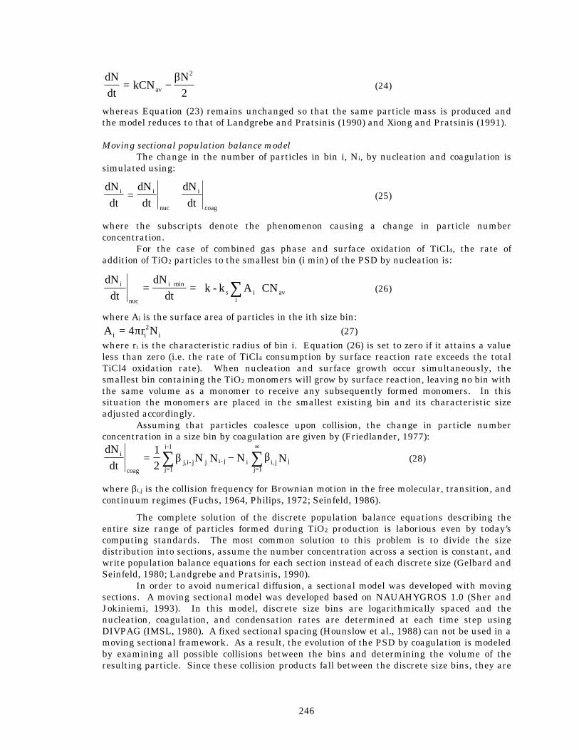
246

dNdt

= −kCNN

av

β 2

2 (24)

whereas Equation (23) remains unchanged so that the same particle mass is produced and the model reduces to that of Landgrebe and Pratsinis (1990) and Xiong and Pratsinis (1991). Moving sectional population balance model The change in the number of particles in bin i, Ni, by nucleation and coagulation is simulated using:

dNdt

i = +dNdt

dNdt

i

nuc

i

coag

(25)

where the subscripts denote the phenomenon causing a change in particle number concentration.

For the case of combined gas phase and surface oxidation of TiCl4, the rate of addition of TiO2 particles to the smallest bin (i min) of the PSD by nucleation is:

dNdt

dNdt

k - k CNi i mins av

nuci

i

A= =

⋅ ∑ (26)

where Ai is the surface area of particles in the ith size bin:

A ri i2= 4π N i (27)

where ri is the characteristic radius of bin i. Equation (26) is set to zero if it attains a value less than zero (i.e. the rate of TiCl4 consumption by surface reaction rate exceeds the total TiCl4 oxidation rate). When nucleation and surface growth occur simultaneously, the smallest bin containing the TiO2 monomers will grow by surface reaction, leaving no bin with the same volume as a monomer to receive any subsequently formed monomers. In this situation the monomers are placed in the smallest existing bin and its characteristic size adjusted accordingly.

Assuming that particles coalesce upon collision, the change in particle number concentration in a size bin by coagulation are given by (Friedlander, 1977): dNdt

= N N N Ni

coag j=1

i-1

j,i- j j i- j ij=1

i, j j12 ∑ ∑−

∞

β β (28)

where βi,j is the collision frequency for Brownian motion in the free molecular, transition, and continuum regimes (Fuchs, 1964, Philips, 1972; Seinfeld, 1986).

The complete solution of the discrete population balance equations describing the entire size range of particles formed during TiO2 production is laborious even by today’s computing standards. The most common solution to this problem is to divide the size distribution into sections, assume the number concentration across a section is constant, and write population balance equations for each section instead of each discrete size (Gelbard and Seinfeld, 1980; Landgrebe and Pratsinis, 1990). In order to avoid numerical diffusion, a sectional model was developed with moving sections. A moving sectional model was developed based on NAUAHYGROS 1.0 (Sher and Jokiniemi, 1993). In this model, discrete size bins are logarithmically spaced and the nucleation, coagulation, and condensation rates are determined at each time step using DIVPAG (IMSL, 1980). A fixed sectional spacing (Hounslow et al., 1988) can not be used in a moving sectional framework. As a result, the evolution of the PSD by coagulation is modeled by examining all possible collisions between the bins and determining the volume of the resulting particle. Since these collision products fall between the discrete size bins, they are

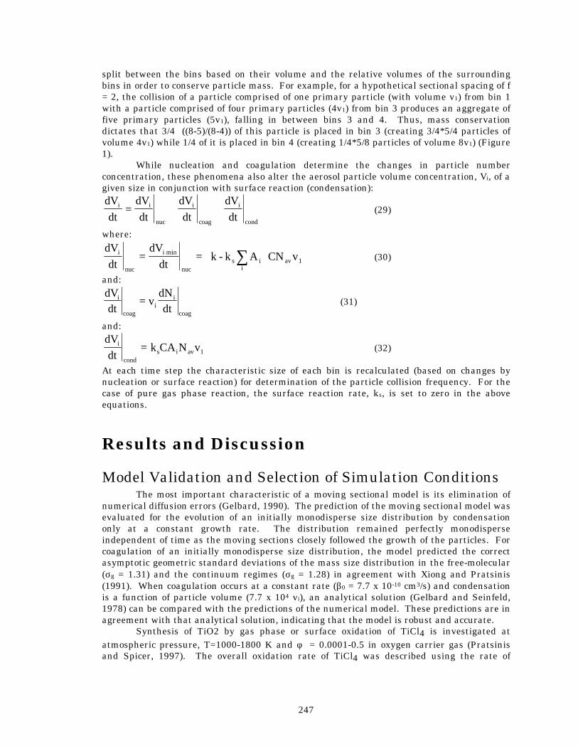
247

split between the bins based on their volume and the relative volumes of the surrounding bins in order to conserve particle mass. For example, for a hypothetical sectional spacing of f = 2, the collision of a particle comprised of one primary particle (with volume v1) from bin 1 with a particle comprised of four primary particles (4v1) from bin 3 produces an aggregate of five primary particles (5v1), falling in between bins 3 and 4. Thus, mass conservation dictates that 3/4 ((8-5)/(8-4)) of this particle is placed in bin 3 (creating 3/4*5/4 particles of volume 4v1) while 1/4 of it is placed in bin 4 (creating 1/4*5/8 particles of volume 8v1) (Figure 1).

While nucleation and coagulation determine the changes in particle number concentration, these phenomena also alter the aerosol particle volume concentration, Vi, of a given size in conjunction with surface reaction (condensation): dVdt

i = + +dVdt

dVdt

dVdt

i

nuc

i

coag

i

cond

(29)

where:

dVdt

dVdt

A vi

nuc

i

nuci

i

= =

⋅ ∑min k - k CNs av 1 (30)

and: dVdt

vdNdt

i

coagi

i

coag

= (31)

and: dVdt

=i

cond

k CA N vs i av 1 (32)

At each time step the characteristic size of each bin is recalculated (based on changes by nucleation or surface reaction) for determination of the particle collision frequency. For the case of pure gas phase reaction, the surface reaction rate, ks, is set to zero in the above equations.


Model Validation and Selection of Simulation Conditions The most important characteristic of a moving sectional model is its elimination of numerical diffusion errors (Gelbard, 1990). The prediction of the moving sectional model was evaluated for the evolution of an initially monodisperse size distribution by condensation only at a constant growth rate. The distribution remained perfectly monodisperse independent of time as the moving sections closely followed the growth of the particles. For coagulation of an initially monodisperse size distribution, the model predicted the correct asymptotic geometric standard deviations of the mass size distribution in the free-molecular (σg = 1.31) and the continuum regimes (σg = 1.28) in agreement with Xiong and Pratsinis (1991). When coagulation occurs at a constant rate (β0 = 7.7 x 10-10 cm3/s) and condensation is a function of particle volume (7.7 x 104 vi), an analytical solution (Gelbard and Seinfeld, 1978) can be compared with the predictions of the numerical model. These predictions are in agreement with that analytical solution, indicating that the model is robust and accurate. Synthesis of TiO2 by gas phase or surface oxidation of TiCl4 is investigated at atmospheric pressure, T=1000-1800 K and φ = 0.0001-0.5 in oxygen carrier gas (Pratsinis and Spicer, 1997). The overall oxidation rate of TiCl4 was described using the rate of

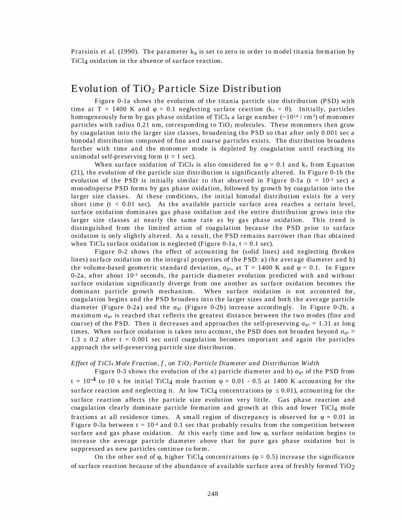
248

Pratsinis et al. (1990). The parameter ks is set to zero in order to model titania formation by TiCl4 oxidation in the absence of surface reaction.

Evolution of TiO2 Particle Size Distribution Figure 0-1a shows the evolution of the titania particle size distribution (PSD) with time at T = 1400 K and φ = 0.1 neglecting surface reaction (ks = 0). Initially, particles homogeneously form by gas phase oxidation of TiCl4 a large number (~1014 / cm3) of monomer particles with radius 0.21 nm, corresponding to TiO2 molecules. These monomers then grow by coagulation into the larger size classes, broadening the PSD so that after only 0.001 sec a bimodal distribution composed of fine and coarse particles exists. The distribution broadens further with time and the monomer mode is depleted by coagulation until reaching its unimodal self-preserving form (t = 1 sec).

When surface oxidation of TiCl4 is also considered for φ = 0.1 and ks from Equation (21), the evolution of the particle size distribution is significantly altered. In Figure 0-1b the evolution of the PSD is initially similar to that observed in Figure 0-1a (t = 10-3 sec) a monodisperse PSD forms by gas phase oxidation, followed by growth by coagulation into the larger size classes. At these conditions, the initial bimodal distribution exists for a very short time (t < 0.01 sec). As the available particle surface area reaches a certain level, surface oxidation dominates gas phase oxidation and the entire distribution grows into the larger size classes at nearly the same rate as by gas phase oxidation. This trend is distinguished from the limited action of coagulation because the PSD prior to surface oxidation is only slightly altered. As a result, the PSD remains narrower than that obtained when TiCl4 surface oxidation is neglected (Figure 0-1a, t = 0.1 sec).

Figure 0-2 shows the effect of accounting for (solid lines) and neglecting (broken lines) surface oxidation on the integral properties of the PSD: a) the average diameter and b) the volume-based geometric standard deviation, σgv, at T = 1400 K and φ = 0.1. In Figure 0-2a, after about 10-3 seconds, the particle diameter evolution predicted with and without surface oxidation significantly diverge from one another as surface oxidation becomes the dominant particle growth mechanism. When surface oxidation is not accounted for, coagulation begins and the PSD broadens into the larger sizes and both the average particle diameter (Figure 0-2a) and the σgv (Figure 0-2b) increase accordingly. In Figure 0-2b, a maximum σgv is reached that reflects the greatest distance between the two modes (fine and coarse) of the PSD. Then it decreases and approaches the self-preserving σgv = 1.31 at long times. When surface oxidation is taken into account, the PSD does not broaden beyond σgv = 1.3 ± 0.2 after t = 0.001 sec until coagulation becomes important and again the particles approach the self-preserving particle size distribution. Effect of TiCl4 Mole Fraction, φ, on TiO2 Particle Diameter and Distribution Width Figure 0-3 shows the evolution of the a) particle diameter and b) σgv of the PSD from t = 10-4 to 10 s for initial TiCl4 mole fraction φ = 0.01 - 0.5 at 1400 K accounting for the surface reaction and neglecting it. At low TiCl4 concentrations (φ ≤ 0.01), accounting for the surface reaction affects the particle size evolution very little. Gas phase reaction and coagulation clearly dominate particle formation and growth at this and lower TiCl4 mole fractions at all residence times. A small region of discrepancy is observed for φ = 0.01 in Figure 0-3a between t = 10-4 and 0.1 sec that probably results from the competition between surface and gas phase oxidation. At this early time and low φ, surface oxidation begins to increase the average particle diameter above that for pure gas phase oxidation but is suppressed as new particles continue to form.

On the other end of φ, higher TiCl4 concentrations (φ = 0.5) increase the significance of surface reaction because of the abundance of available surface area of freshly formed TiO2

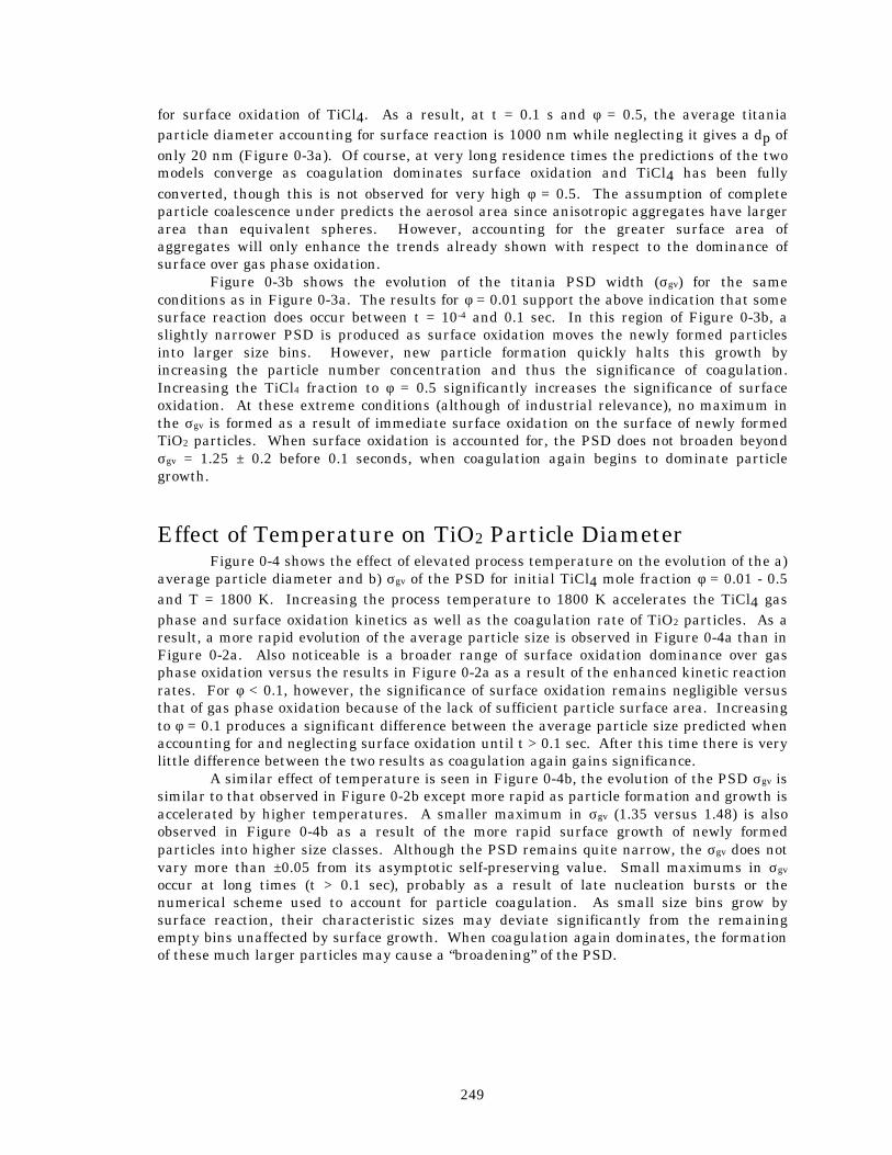
249

for surface oxidation of TiCl4. As a result, at t = 0.1 s and φ = 0.5, the average titania particle diameter accounting for surface reaction is 1000 nm while neglecting it gives a dp of only 20 nm (Figure 0-3a). Of course, at very long residence times the predictions of the two models converge as coagulation dominates surface oxidation and TiCl4 has been fully converted, though this is not observed for very high φ = 0.5. The assumption of complete particle coalescence under predicts the aerosol area since anisotropic aggregates have larger area than equivalent spheres. However, accounting for the greater surface area of aggregates will only enhance the trends already shown with respect to the dominance of surface over gas phase oxidation. Figure 0-3b shows the evolution of the titania PSD width (σgv) for the same conditions as in Figure 0-3a. The results for φ = 0.01 support the above indication that some surface reaction does occur between t = 10-4 and 0.1 sec. In this region of Figure 0-3b, a slightly narrower PSD is produced as surface oxidation moves the newly formed particles into larger size bins. However, new particle formation quickly halts this growth by increasing the particle number concentration and thus the significance of coagulation. Increasing the TiCl4 fraction to φ = 0.5 significantly increases the significance of surface oxidation. At these extreme conditions (although of industrial relevance), no maximum in the σgv is formed as a result of immediate surface oxidation on the surface of newly formed TiO2 particles. When surface oxidation is accounted for, the PSD does not broaden beyond σgv = 1.25 ± 0.2 before 0.1 seconds, when coagulation again begins to dominate particle growth.

Effect of Temperature on TiO2 Particle Diameter Figure 0-4 shows the effect of elevated process temperature on the evolution of the a)

average particle diameter and b) σgv of the PSD for initial TiCl4 mole fraction φ = 0.01 - 0.5 and T = 1800 K. Increasing the process temperature to 1800 K accelerates the TiCl4 gas phase and surface oxidation kinetics as well as the coagulation rate of TiO2 particles. As a result, a more rapid evolution of the average particle size is observed in Figure 0-4a than in Figure 0-2a. Also noticeable is a broader range of surface oxidation dominance over gas phase oxidation versus the results in Figure 0-2a as a result of the enhanced kinetic reaction rates. For φ < 0.1, however, the significance of surface oxidation remains negligible versus that of gas phase oxidation because of the lack of sufficient particle surface area. Increasing to φ = 0.1 produces a significant difference between the average particle size predicted when accounting for and neglecting surface oxidation until t > 0.1 sec. After this time there is very little difference between the two results as coagulation again gains significance.

A similar effect of temperature is seen in Figure 0-4b, the evolution of the PSD σgv is similar to that observed in Figure 0-2b except more rapid as particle formation and growth is accelerated by higher temperatures. A smaller maximum in σgv (1.35 versus 1.48) is also observed in Figure 0-4b as a result of the more rapid surface growth of newly formed particles into higher size classes. Although the PSD remains quite narrow, the σgv does not vary more than ±0.05 from its asymptotic self-preserving value. Small maximums in σgv occur at long times (t > 0.1 sec), probably as a result of late nucleation bursts or the numerical scheme used to account for particle coagulation. As small size bins grow by surface reaction, their characteristic sizes may deviate significantly from the remaining empty bins unaffected by surface growth. When coagulation again dominates, the formation of these much larger particles may cause a “broadening” of the PSD.

250

Comparison with Monodisperse Model Results Though the moving sectional model provides a robust description of TiO2 formation

and growth, the average computational load required makes it worth examining the predictions of a monodisperse model of TiO2 aerosol synthesis. Figure 0-5 shows the predictions of the monodisperse and population balance models for the same conditions as in Figure 0-4a. The monodisperse model is in good agreement with the moving sectional model with respect to the formation and growth of titania by only gas phase oxidation and coagulation. However, when surface oxidation is considered, the monodisperse model slightly over predicts its significance, predicting a broader range of time when surface oxidation is dominant. A monodisperse model over predicts the significance of surface reaction because it over predicts initial particle growth by coagulation, leading to an enhanced particle surface area and, consequently, an over prediction of the surface reaction rates (Warren and Seinfeld, 1985). However, the overall good agreement observed in Figure 0-5 emphasizes the usefulness of simple, monodisperse models for the prediction of aerosol dynamics.

Comparison with Alternative Models of Surface Oxidation Figure 0-6 compares the results of the moving sectional model of this study with the

results produced assuming that the rate of gas phase particle formation is given by Rg = -kC and that the total rate of particle formation and growth is given by R = -(ksAC + kC) (Jain et al., 1997). This assumption is shown in Figure 0-6 to under predict the significance of surface oxidation, thus over predicting the significance of gas phase oxidation at later times. This result, along with the use of a lognormal approximation of the PSD, may explain the conclusion of Jain et al. (1997) that surface oxidation was insignificant in TiO2 production by TiCl4 oxidation. While the lognormal model of Jain et al. (1997) allows for consideration of particle size distribution polydispersity, its assumption of a lognormal PSD is limited in its ability to describe particle behavior following a nucleation burst. As monomers form by gas phase reaction, then grow by coagulation, a bimodal PSD is formed (Figure 0-1) that is not well described by moment techniques (Xiong and Pratsinis, 1991).

Criteria for TiO2 Synthesis by Coagulation or Surface Growth It is often desired to practically produce a titania particle size distribution below a maximum width depending on the final application. The model developed in this work makes it possible to estimate the range of conditions when a narrower PSD is produced as a result of the dominance of surface over gas phase oxidation. Figure 0-7 shows a diagram of the initial TiCl4 mole fraction, φ, and product TiO2 diameter, dp, in which particle growth is dominated either by surface oxidation or gas phase oxidation of TiCl4 at various temperatures. Each line is a contour of constant particle size distribution widths in which the model that accounts for surface oxidation predicts a σgv 5% smaller than that of the model that neglects surface reaction (in some cases as small as a σgv ≈ 1.25). Figure 0-7 shows that surface reaction has a significant effect on titania growth at high TiCl4 mole fractions, φ > 0.01, for particle synthesis in the range of 70-100 nm. Outside this range, coagulation dominates, producing particles with broader, self-preserving size distributions. The surface growth region of the diagram inside the U shaped curves identifies conditions where particles of narrow size distribution and limited extent of agglomeration can be made. This is in agreement with the results of Pratsinis (1988) who showed that for simultaneous

251

coagulation and condensation (surface reaction), aerosol particles have size distributions narrower than that predicted by the self-preserving theory (Friedlander, 1977).

Conclusions A moving sectional population balance model was developed that eliminates

numerical diffusion errors while accounting for simultaneous nucleation, coagulation, and surface reaction during the synthesis of TiO2. Including surface reaction in models of TiO2 formation increases the average particle size and narrows the product particle size distribution above TiCl4 volume fraction φ = 10-2 versus pure gas phase reaction, with this effect increasing with increasing process temperature. The population balance model is shown to be in good agreement with an existing monodisperse model of TiO2 formation and growth, although the monodisperse model slightly overpredicts the effect of surface oxidation at low T and φ. Regions of surface oxidation-dominated particle growth are identified based on the criterion of a 5% deviation from the geometric standard deviation of the TiO2 particle size distribution neglecting surface oxidation. TiO2 synthesis at high precursor concentration and temperature results in the production of larger particles with a narrower size distribution.

Acknowledgments We acknowledge support by the National Science Foundation, Grant # CTS-9619392,

and Dr. Jorma Jokiniemi (VTT) for providing the NAUAHYGROS source code.

252

References Friedlander, S. K., Smoke, Dust, and Haze, Wiley, New York, (1977). Fuchs, N. A., The Mechanics of Aerosols, Pergamon Press, Elmsford, NY, 1964. Gelbard, F. and Seinfeld, J. H., “Simulation of Multicomponent Aerosol Dynamics,” J. Colloid

Interface Sci., 78, 485-501 (1980). Gelbard, F., “Modeling Multicomponent Aerosol Particle Growth by Vapor Condensation,”

Aerosol Sci. Tech., 12, 399-412 (1990). Gelbard, F., Tambour, Y., and Seinfeld, J. H., “Sectional Representations for Simulating

Aerosol Dynamics,” J. Colloid Interface Sci., 76, 541-556 (1980). Ghoshtagore, R. N., “Mechanism of Heterogeneous Deposition of Thin Film Rutile,” J.

Electrochem Soc.: Solid State Science, 117, 529-534 (1970). Hounslow, M. J., Ryall, R. L., and Marshall, V. R., "A Discretized Population Balance for

Nucleation, Growth, and Aggregation," AIChE J., 34, 1821-1832 (1988). IMSL, IMSL Contents Document, 8th ed. International Mathematical and Statistical

Libraries, Houston (1980). Jacobson, M. Z. and Turco, R. P., “Simulating Condensation Growth, Evaporation, and

Coagulation of Aerosols Using a Combined Moving and Stationary Size Grid,” Aerosol Sci. Tech., 22, 73-92 (1995).

Jain, S., Kodas, T. T., Wu, M. K., and Preston, P., “Role of Surface Reaction in Aerosol Synthesis of Titanium Dioxide,” J. Aerosol Sci., 28, 133-146 (1997).

Kim K.S., S.E. Pratsinis, "Modeling and Analysis of Modified Chemical Vapor Deposition of Optical Fiber Preforms", Chem. Eng. Sci., 44, 2475-2482 (1989).

Kim, Y. P. and Seinfeld, J. H., “Simulation of Multicomponent Aerosol Condensation by the Moving Sectional Method,” J. Colloid Interface Sci., 135, 185-199 (1990).

Kruis F.E., K. Kusters, S.E. Pratsinis, B. Scarlett, "A Simple Model for the Evolution of the Characteristics of Aggregate Particles undergoing Coagulation and Sintering" Aerosol Sci. Technol. 19, 514-526 (1993).

Landgrebe, J. D. And Pratsinis, S. E., “A Discrete-Sectional Model for Powder Production by Gas-Phase Chemical Reaction and Aerosol Coagulation in the Free-Molecular Regime,” J. Colloid Interface Sci., 139, 63-86 (1990).

Ollis, D. F., Hsiao, C.-Y., Budiman, L., and Lee, C.-L., “Heterogeneous Photoassisted Catalysis: Conversions of Perchloroethylene, Dichloroethane, Chloroacteic Acids, and Chlorobenzenes,” J. Catalysis., 88, 89-96 (1984).

Phillips, W.F. "Drag on a Small Sphere Moving through a Gas", Phys. Fluids, 18, 1089-1093 (1975).

Pratsinis, S. E., H. Bai, P. Biswas, M. Frenklach and S. V. R. Mastrangelo, “Kinetics of TiCl4 Oxidation”, J. Am. Ceram. Soc., 73, 2158-2162 (1990).

Pratsinis, S.E. "Simultaneous Nucleation, Condensation and Coagulation in Aerosol Reactors", J. Colloid Interface Sci., 124, 416-427 (1988).

Pratsinis, S. E. and Spicer, P. T., “Competition between Gas Phase and Surface Oxidation of TiCl4 during Synthesis of TiO2 Particles,” Chemical Engineering Science (in press, 1997).

Seinfeld, J. H., Atmospheric Chemistry and Physics of Air Pollution, Wiley, New York, 1986. Sher, R. and Jokiniemi, J., “NAUAHYGROS 1.0: A Code for Calculating the Behaviour of

Aerosols in Nuclear Plant Containments Following a Severe Accident,” User's Manual: EPRI TR-102775, July 1993.

Tan, Y.-S., Dou, L.-Q., Lu, D.-S., and Wu, D., “Coated Silica as Support for Platinum Catalyst I. Coating of Silica with Alumina, Titania, and Lanthana,” J. Catalysis, 129, 447-456 (1991).

Warren, D. R. and Seinfeld, J. H., "Prediction of Aerosol Concentration Resulting from a Burst of Nucleation," J. Colloid Interface Sci., 105, 136-142 (1985).

253

Xiong Y. and S. E. Pratsinis, “Gas Phase Production of Particles in Reactive Turbulent Flows,” J. Aerosol Sci., 22, 637-55 (1991).

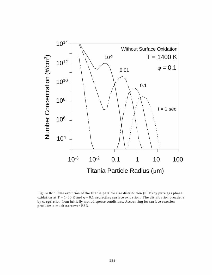
254

Figure 0-1: Time evolution of the titania particle size distribution (PSD) by pure gas phase oxidation at T = 1400 K and φ = 0.1 neglecting surface oxidation. The distribution broadens by coagulation from initially monodisperse conditions. Accounting for surface reaction produces a much narrower PSD.

Titania Particle Radius (µm)

Num

ber

Con

cent

ratio

n (#

/cm

3 )

t = 1 sec

0.01

10-3

10-3 110-2 0.1 10010

Without Surface Oxidation

T = 1400 K

φ = 0.1

0.1

106

104

1012

1014

108

1010

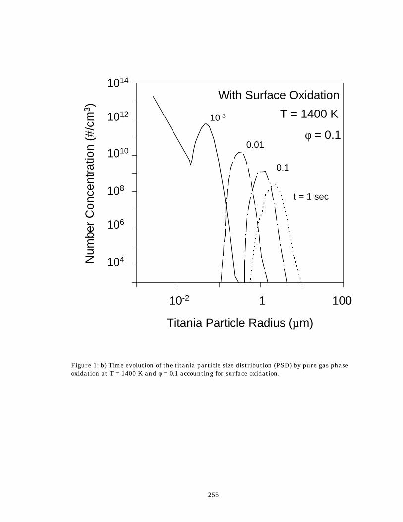
255

Figure 1: b) Time evolution of the titania particle size distribution (PSD) by pure gas phase oxidation at T = 1400 K and φ = 0.1 accounting for surface oxidation.

Titania Particle Radius (µm)

Num

ber

Con

cent

ratio

n (#

/cm

3 )

t = 1 sec

0.01

0.1

110-2 100

With Surface Oxidation

T = 1400 K

φ = 0.1

10-3

104

106

1012

1014

108

1010

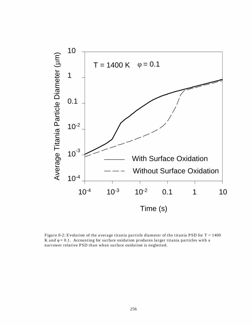
256

Figure 0-2: Evolution of the average titania particle diameter of the titania PSD for T = 1400 K and φ = 0.1. Accounting for surface oxidation produces larger titania particles with a narrower relative PSD than when surface oxidation is neglected.

Time (s)

Ave

rage

Tita

nia

Par

ticle

Dia

met

er (

µm)

T = 1400 K

1010.1

φ = 0.1



10-210-3

1

0.1

10-2

10-3

10-4

10

10-4

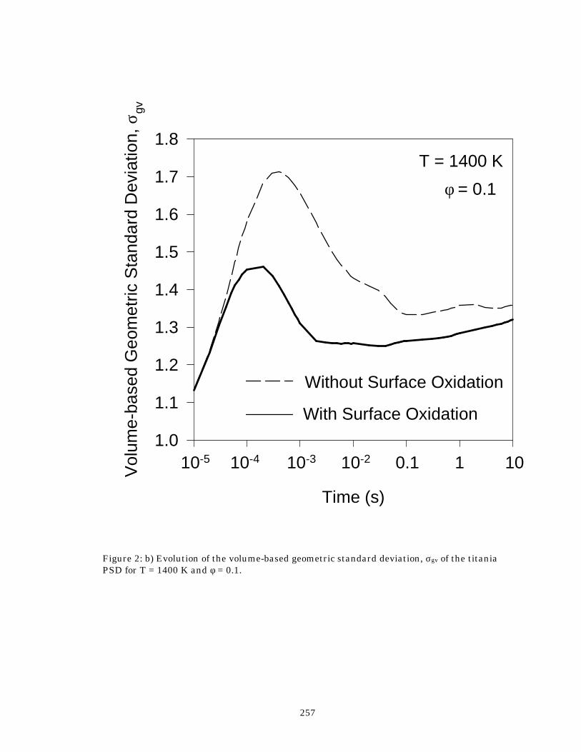
257

Figure 2: b) Evolution of the volume-based geometric standard deviation, σgv of the titania PSD for T = 1400 K and φ = 0.1.

Time (s)

Vol

ume-

base

d G

eom

etric

Sta

ndar

d D

evia

tion,

σgv

1.0

1.1

1.2

1.3

1.4

1.5

1.6

1.7

1.8

10-4 1010.110-210-310-5

T = 1400 K

φ = 0.1



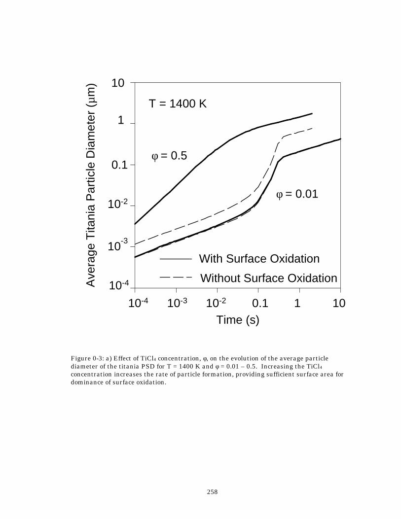
258

Figure 0-3: a) Effect of TiCl4 concentration, φ, on the evolution of the average particle diameter of the titania PSD for T = 1400 K and φ = 0.01 – 0.5. Increasing the TiCl4 concentration increases the rate of particle formation, providing sufficient surface area for dominance of surface oxidation.

Time (s)

Ave

rage

Tita

nia

Par

ticle

Dia

met

er (

µm)

T = 1400 K1

0.1

10-2

10-3

10-4

10-4 1010.110-210-3

φ = 0.5

φ = 0.01

10



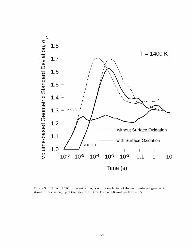
259

Figure 3: b) Effect of TiCl4 concentration, φ, on the evolution of the volume-based geometric standard deviation, σgv of the titania PSD for T = 1400 K and φ = 0.01 – 0.5.

Time (s)

Vol

ume-

base

d G

eom

etric

Sta

ndar

d D

evia

tion,

σgv

1.0

1.1

1.2

1.3

1.4

1.5

1.6

1.7

1.8

10-4 1010.110-210-310-5

T = 1400 K

φ = 0.01

φ = 0.5

10-6

with Surface Oxidation

without Surface Oxidation

260

Figure 0-4: a) Effect of process temperature on the evolution of the average particle diameter of the titania PSD for T = 1800 K and φ = 0.01 – 0.1. Increasing the temperature increases the surface and gas phase oxidation kinetics, significantly accelerating particle growth by surface reaction.

Time (s)

Ave

rage

Tita

nia

Par

ticle

Dia

met

er (

µm)

T = 1800 K

1

0.1

10-2

10-3

10-4

10-4 1010.110-210-3

φ = 0.1φ = 0.01



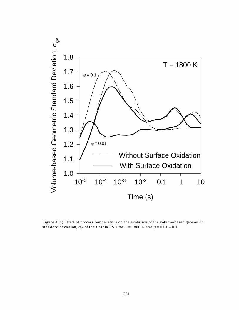
261

Figure 4: b) Effect of process temperature on the evolution of the volume-based geometric standard deviation, σgv of the titania PSD for T = 1800 K and φ = 0.01 – 0.1.

Time (s)

Vol

ume-

base

d G

eom

etric

Sta

ndar

d D

evia

tion,

σgv

1.0

1.1

1.2

1.3

1.4

1.5

1.6

1.7

1.8

10-4 1010.110-210-310-5

T = 1800 K

φ = 0.01

φ = 0.1

With Surface OxidationWithout Surface Oxidation

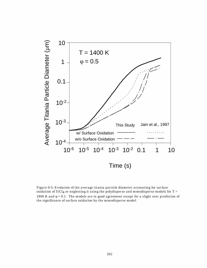
262

Figure 0-5: Evolution of the average titania particle diameter accounting for surface oxidation of TiCl4 or neglecting it using the polydisperse and monodisperse models for T = 1800 K and φ = 0.1. The models are in good agreement except for a slight over prediction of the significance of surface oxidation by the monodisperse model.

Time (s)

Ave

rage

Tita

nia

Par

ticle

Dia

met

er (

µm)

T = 1400 Kφ = 0.5

10

1

0.1

10-2

10-3

10-4

10-6 10-5 10-310-4 10-2 0.1 1 10

This Study

w/ Surface Oxidation

Jain et al., 1997

w/o Surface Oxidation

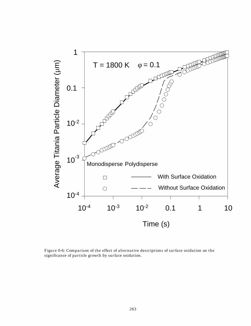
263

Figure 0-6: Comparison of the effect of alternative descriptions of surface oxidation on the significance of particle growth by surface oxidation.

Time (s)

Ave

rage

Tita

nia

Par

ticle

Dia

met

er (

µm)

T = 1800 K

1

0.1

10-2

10-3

10-4

10-4 1010.110-210-3

φ = 0.1

Monodisperse Polydisperse



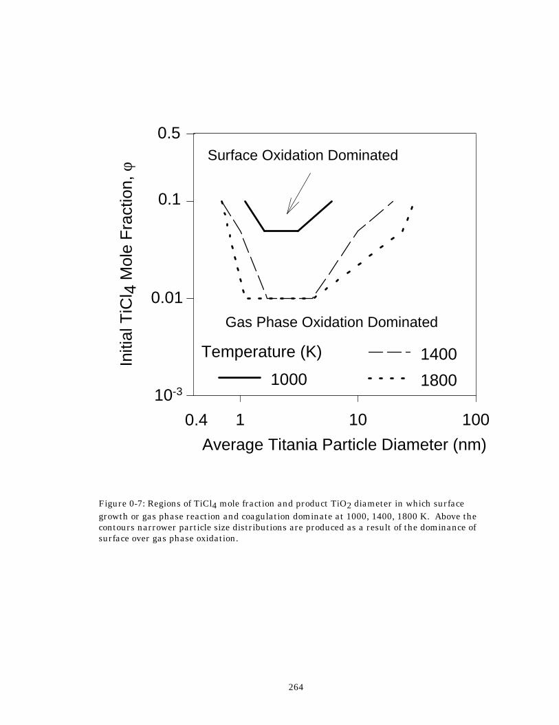
264

Figure 0-7: Regions of TiCl4 mole fraction and product TiO2 diameter in which surface growth or gas phase reaction and coagulation dominate at 1000, 1400, 1800 K. Above the contours narrower particle size distributions are produced as a result of the dominance of surface over gas phase oxidation.

Average Titania Particle Diameter (nm)1 10 100

Initi

al T

iCl 4

Mol

e F

ract

ion,

φ

0.1

0.01

10-3

0.5

0.4

Gas Phase Oxidation Dominated

Surface Oxidation Dominated

Temperature (K)

1000

1400

1800

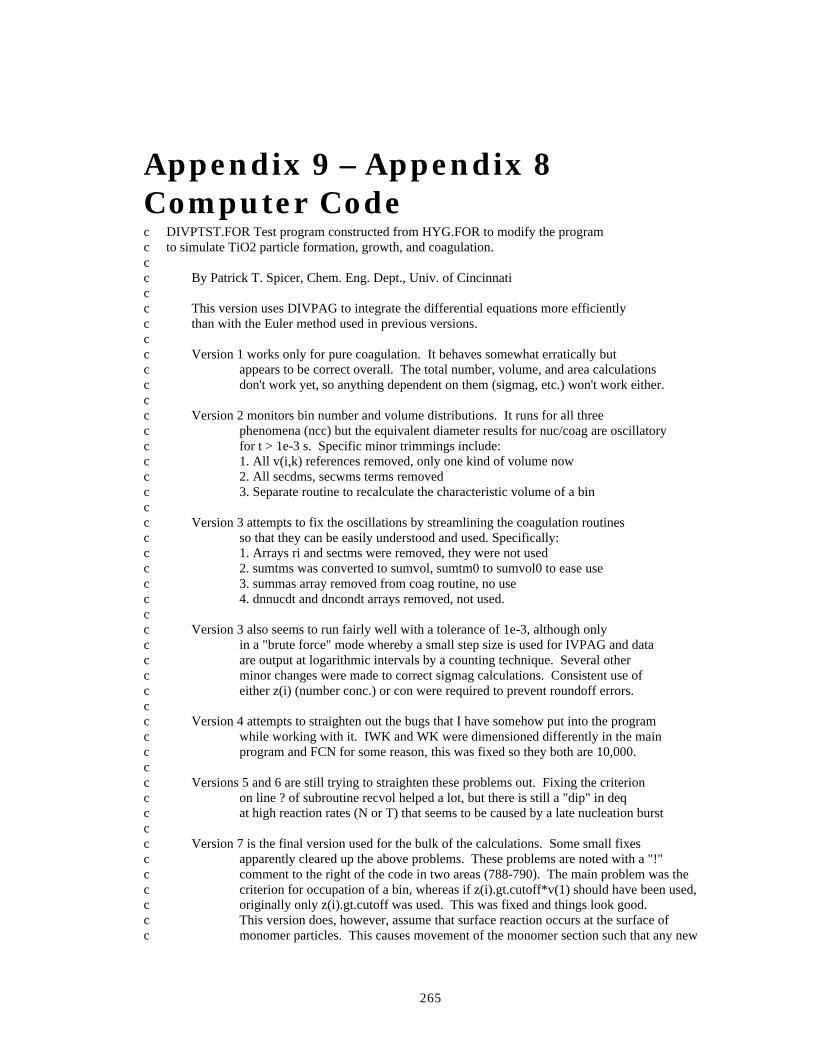
265

Appendix 9 – Appendix 8 Computer Code c DIVPTST.FOR Test program constructed from HYG.FOR to modify the program c to simulate TiO2 particle formation, growth, and coagulation. c c By Patrick T. Spicer, Chem. Eng. Dept., Univ. of Cincinnati c c This version uses DIVPAG to integrate the differential equations more efficiently c than with the Euler method used in previous versions. c c Version 1 works only for pure coagulation. It behaves somewhat erratically but c appears to be correct overall. The total number, volume, and area calculations c don't work yet, so anything dependent on them (sigmag, etc.) won't work either. c c Version 2 monitors bin number and volume distributions. It runs for all three c phenomena (ncc) but the equivalent diameter results for nuc/coag are oscillatory c for t > 1e-3 s. Specific minor trimmings include: c 1. All v(i,k) references removed, only one kind of volume now c 2. All secdms, secwms terms removed c 3. Separate routine to recalculate the characteristic volume of a bin c c Version 3 attempts to fix the oscillations by streamlining the coagulation routines c so that they can be easily understood and used. Specifically: c 1. Arrays ri and sectms were removed, they were not used c 2. sumtms was converted to sumvol, sumtm0 to sumvol0 to ease use c 3. summas array removed from coag routine, no use c 4. dnnucdt and dncondt arrays removed, not used. c c Version 3 also seems to run fairly well with a tolerance of 1e-3, although only c in a "brute force" mode whereby a small step size is used for IVPAG and data c are output at logarithmic intervals by a counting technique. Several other c minor changes were made to correct sigmag calculations. Consistent use of c either z(i) (number conc.) or con were required to prevent roundoff errors. c c Version 4 attempts to straighten out the bugs that I have somehow put into the program c while working with it. IWK and WK were dimensioned differently in the main c program and FCN for some reason, this was fixed so they both are 10,000. c c Versions 5 and 6 are still trying to straighten these problems out. Fixing the criterion c on line ? of subroutine recvol helped a lot, but there is still a "dip" in deq c at high reaction rates (N or T) that seems to be caused by a late nucleation burst c c Version 7 is the final version used for the bulk of the calculations. Some small fixes c apparently cleared up the above problems. These problems are noted with a "!" c comment to the right of the code in two areas (788-790). The main problem was the c criterion for occupation of a bin, whereas if z(i).gt.cutoff*v(1) should have been used, c originally only z(i).gt.cutoff was used. This was fixed and things look good. c This version does, however, assume that surface reaction occurs at the surface of c monomer particles. This causes movement of the monomer section such that any new

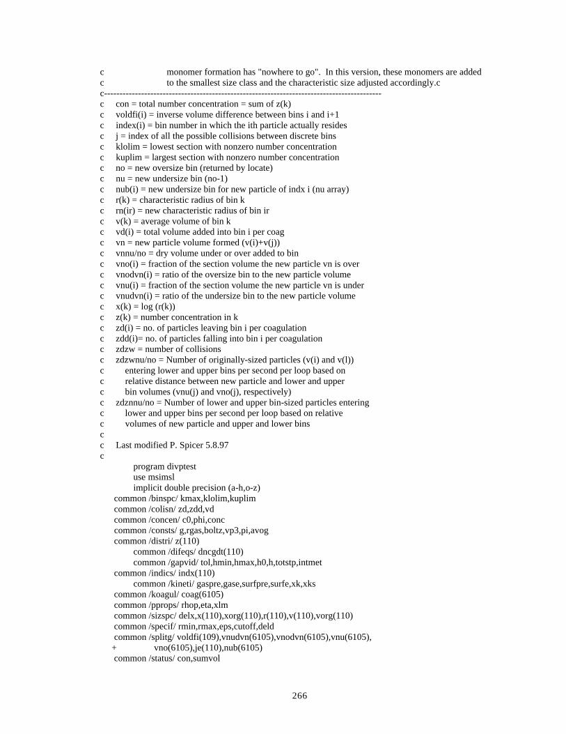
266

c monomer formation has "nowhere to go". In this version, these monomers are added c to the smallest size class and the characteristic size adjusted accordingly.c c------------------------------------------------------------------------------------------ c con = total number concentration = sum of z(k) c voldfi(i) = inverse volume difference between bins i and i+1 c index(i) = bin number in which the ith particle actually resides c j = index of all the possible collisions between discrete bins c klolim = lowest section with nonzero number concentration c kuplim = largest section with nonzero number concentration c no = new oversize bin (returned by locate) c nu = new undersize bin (no-1) c nub(i) = new undersize bin for new particle of indx i (nu array) c r(k) = characteristic radius of bin k c rn(ir) = new characteristic radius of bin ir c v(k) = average volume of bin k c vd(i) = total volume added into bin i per coag c vn = new particle volume formed (v(i)+v(j)) c vnnu/no = dry volume under or over added to bin c vno(i) = fraction of the section volume the new particle vn is over c vnodvn(i) = ratio of the oversize bin to the new particle volume c vnu(i) = fraction of the section volume the new particle vn is under c vnudvn(i) = ratio of the undersize bin to the new particle volume c x(k) = log (r(k)) c z(k) = number concentration in k c zd(i) = no. of particles leaving bin i per coagulation c zdd(i)= no. of particles falling into bin i per coagulation c zdzw = number of collisions c zdzwnu/no = Number of originally-sized particles (v(i) and v(l)) c entering lower and upper bins per second per loop based on c relative distance between new particle and lower and upper c bin volumes (vnu(j) and vno(j), respectively) c zdznnu/no = Number of lower and upper bin-sized particles entering c lower and upper bins per second per loop based on relative c volumes of new particle and upper and lower bins c c Last modified P. Spicer 5.8.97 c program divptest use msimsl implicit double precision (a-h,o-z) common /binspc/ kmax,klolim,kuplim common /colisn/ zd,zdd,vd common /concen/ c0,phi,conc common /consts/ g,rgas,boltz,vp3,pi,avog common /distri/ z(110) common /difeqs/ dncgdt(110) common /gapvid/ tol,hmin,hmax,h0,h,totstp,intmet common /indics/ indx(110) common /kineti/ gaspre,gase,surfpre,surfe,xk,xks common /koagul/ coag(6105) common /pprops/ rhop,eta,xlm common /sizspc/ delx,x(110),xorg(110),r(110),v(110),vorg(110) common /specif/ rmin,rmax,eps,cutoff,deld common /splitg/ voldfi(109),vnudvn(6105),vnodvn(6105),vnu(6105), + vno(6105),je(110),nub(6105) common /status/ con,sumvol

267

common /switch/ knuc,kcoag,kcond,koutpu common /temper/ temp common /timedt/ t,tmax,deltat common /totmas/ con0,sumvol0 common /wriout/ toutpu,icount logical knuc,kcoag,kcond,koutpu c dimension zd(110),zdd(110),vd(110),zp(110),param(100),iwk(10000), + wk(10000) external fcn,fcnj c open (unit = 10, file = 'sd.prn') open (unit = 9, file = 'deq.prn') open (unit = 8, file = 'sig.prn') open (unit = 7, file = 'nva.prn') open (unit = 3, file = 'divptest.in') c c@@@@@@@@@@@@@@@@@@@@ Start of Main Program @@@@@@@@@@@@@@@@@@@@@@@@@@@@ c call outtim(0) c Read in parameters from input file call input c Set up initial size distribution call initsd c Initialize size and mass arrays call initia c Set up bin sizes call setbin c Determine where particles go when they coagulate call split c Initialize time t = 0.d0 c Initialize DIVPAG parameters c Initial value of the internal step size, h c param(1) = h0 c Minimum value of the internal step size, h param(2) = hmin c Maximum value of the internal step size, h param(3) = hmax c Maximum # of internal time steps param(4) = totstp c Integration method (1 = Adams Moulton 2 = Gear's Backward Dif.) param(12) = intmet c Nonlinear solver method (1 = Chord method with user-provided Jacobian) c param(13) = 1 c Number of equations to solve ieq = 2*kmax c Initialize counter ifwrite = 1 factor = 1 lchange = 10 lcount = 0 c++++++++++++++++++++++Start of Time Loop+++++++++++++++++++++++++++++++ ido = 1 100 tend = t + h0

268

lcount = lcount + 1 c Call ODE integrator call divpag(ido,ieq,fcn,fcnj,wk,t,tend,tol,param,z) c c Output size distribution parameters to files c if (lcount.eq.ifwrite) then if (koutpu) then call outpsd endif ifwrite = ifwrite + factor if (ifwrite.eq.lchange) then factor = factor*10 lchange = lchange*10 endif endif c if(t.lt.tmax) goto 100 ido = 3 call divpag(ido,ieq,fcn,fcnj,wk,t,tend,tol,param,z) c++++++++++++++++++++++End of Time Loop++++++++++++++++++++++++++++++++++ c call outpar call outtim(1) c stop end c c@@@@@@@@@@@@@@@@@@@@ End of Main Program @@@@@@@@@@@@@@@@@@@@@@@@@@@@@@@ c------------------------------------------------------------------------ c ODEs to integrate (Population balance equations) c------------------------------------------------------------------------ subroutine fcn(ieq,wk,z,zp) implicit double precision (a-h,o-z) common /binspc/ kmax,klolim,kuplim common /difeqs/ dncgdt(110) common /indics/ indx(110) common /pprops/ rhop,eta,xlm common /sizspc/ delx,x(110),xorg(110),r(110),v(110),vorg(110) common /specif/ rmin,rmax,eps,cutoff,deld common /status/ con,sumvol common /switch/ knuc,kcoag,kcond,koutpu common /timedt/ t,tmax,deltat dimension z(110),zp(110),wk(10000),iwk(10000) logical knuc,kcoag,kcond,koutpu c c Coagulation rates of existing particles c if (kcoag) then call split call coagul c c Change in particle number balance by coagulation c

269

do i = 1,kmax zp(i) = dncgdt(i) enddo c c Change in particle volume balance by coagulation c do j = kmax + 1,2*kmax zp(j) = dncgdt(j - kmax)*v(j - kmax) enddo endif c c Change in particle volume balance by condensation c if (kcond) then do i = kmax + klolim,kmax + kuplim if (i.ne.indx(1)) then !New zp(i) = zp(i) + z(i - kmax)*srfrat(r(i - kmax)) endif !New enddo endif c c Nucleation term added to number and volume balance of lowest bin c if (knuc) then zp(indx(1)) = zp(indx(1)) + ratnuc(t) zp(kmax + indx(1)) = zp(kmax + indx(1)) + ratnuc(t)*vorg(1) endif c c Zero any negative or low number concentrations c do i = 1,kmax if(z(i).lt.cutoff) then z(i) = 0.d0 endif if(z(i + kmax).lt.cutoff*vorg(1)) then !This was ...cutoff*v(1).. z(i + kmax) = 0.d0 endif enddo c c Calculate the new characteristic volume of the bins by nucleation/condensation call recvol c Re-order the indices of the bins call indxx(kmax,r,indx) c Re-determine the location of new particles call split c Re-determine the limiting bins call occbin c Recalculate the total number and volume present sumvol = 0.d0 con = 0.d0 do k = 1, kmax con = con + z(k) sumvol = sumvol + z(k + kmax) enddo c return

270

end c------------------------------------------------------------------------ c Read parameters from input file c------------------------------------------------------------------------ subroutine input implicit double precision (a-h,o-z) common /binspc/ kmax,klolim,kuplim common /concen/ c0,phi,conc common /gapvid/ tol,hmin,hmax,h0,h,totstp,intmet common /specif/ rmin,rmax,eps,cutoff,deld common /switch/ knuc,kcoag,kcond,koutpu common /temper/ temp common /timedt/ t,tmax,deltat logical knuc,kcoag,kcond,koutpu c read(3,*)phi read(3,*)temp read(3,*)tmax read(3,*)cutoff read(3,*)tol read(3,*)hmin read(3,*)hmax read(3,*)h0 read(3,*)totstp read(3,*)intmeth read(3,*)rmin read(3,*)rmax read(3,*)kmax read(3,*)knuc read(3,*)kcoag read(3,*)kcond read(3,*)koutpu c return end c-------------------------------------------------------------------- c Set values of the initial size distributions c-------------------------------------------------------------------- subroutine initsd implicit double precision (a-h,o-z) common /binspc/ kmax,klolim,kuplim common /distri/ z(110) common /sizspc/ delx,x(110),xorg(110),r(110),v(110),vorg(110) c do 35 k = 1,kmax z(k) = 0.d0 35 continue c do 45 i = kmax + 1, 2*kmax z(i) = z(i - kmax)*v(i - kmax) 45 continue c c z(1) = 1.d8 c z(1 + kmax) = z(1)*v(1) c return

271

end c---------------------------------------------------------------------- c Initialize variables and arrays c---------------------------------------------------------------------- subroutine initia implicit double precision (a-h,o-z) common /binspc/ kmax,klolim,kuplim common /concen/ c0,phi,conc common /consts/ g,rgas,boltz,vp3,pi,avog common /distri/ z(110) common /gapvid/ tol,hmin,hmax,h0,h,totstp,intmet common /indics/ indx(110) common /kineti/ gaspre,gase,surfpre,surfe,xk,xks common /pprops/ rhop,eta,xlm common /sizspc/ delx,x(110),xorg(110),r(110),v(110),vorg(110) common /specif/ rmin,rmax,eps,cutoff,deld common /splitg/ voldfi(109),vnudvn(6105),vnodvn(6105),vnu(6105), + vno(6105),je(110),nub(6105) common /status/ con,sumvol common /temper/ temp c c Constants initialized c g = 981.d0 rgas = 8.31451d7 boltz = 1.3804d-16 pi = 3.14159265d0 vp3 = 4.d0/3.d0*pi p = 1.01325d6 avog = 6.022137d23 c TiO2 particles xmwp = 80.d0 rhop = 4.26d0 c Arrhenius constant gas phase reaction (Pratsinis et al., 1990) gase = 10680.12d0 gaspre = 8.26d04 c Arrhenius constant surface reaction (Ghoshtagore, 1970) surfe = 8981.21d0 surfpre = 4900.d0 c Calculate rate constants xk = gaspre*dexp(-gase/temp) xks = surfpre*dexp(-surfe/temp) c c Viscosity data for O2 (Reid, Prausnitz, and Poling, 1988) xmwg = 31.9988d0 sigmavis = 3.467d0 epsovk = 106.7d0 xa = 1.16145d0 xb = 0.14874d0 xc = 0.52487d0 xd = 0.77320d0 xe = 2.16178d0 xf = 2.43787d0 c c Calculate initial concentration of TiCl4 based on input vol. fract. c

272

c0 = phi*273.d0/temp/22400.d0 c c Material properties c c Calculate gas viscosity, density, and mean free path c (Reid, Prausnitz, and Poling, 1988) c tstar = temp/epsovk omegav = xa/tstar**xb + xc/dexp(xd*tstar) + xe/dexp(xf*tstar) rhog = p*xmwg/rgas/temp c c (cgs units only, i.e. g/mol, etc.) c eta = 2.669d-5*dsqrt(xmwg*temp)/omegav/sigmavis**2.d0 xnu = eta/rhog xlm = xnu*dsqrt(pi*xmwg/2.d0/rgas/temp) c c Initialize counting variables (lowest and highest occupied bins) c klolim = 1 kuplim = kmax c c Index of every possible collision between number bins c do 10 k = 1,kmax indx(k) = k je(k) = (k-1)*kmax - ((k - 1)*(k - 2))/2 - k + 1 10 continue c return end c--------------------------------------------------------------------- c Initialize the size bins according to the choice of the number of c sections, the maximum size, and the minimum size. c--------------------------------------------------------------------- subroutine setbin implicit double precision (a-h,o-z) common /binspc/ kmax,klolim,kuplim common /consts/ g,rgas,boltz,vp3,pi,avog common /distri/ z(110) common /pprops/ rhop,eta,xlm common /sizspc/ delx,x(110),xorg(110),r(110),v(110),vorg(110) common /specif/ rmin,rmax,eps,cutoff,deld common /status/ con,sumvol common /totmas/ con0,sumvol0 c x(1) = dlog(rmin) xorg(1) = x(1) x(kmax) = dlog(rmax) xorg(kmax) = x(kmax) kmaxx = kmax - 1 r(1) = rmin r(kmax) = rmax delx = (x(kmax) - x(1))/kmaxx c do 10 k = 2,kmaxx

273

x(k) = x(k-1) + delx xorg(k) = x(k) r(k) = dexp(x(k)) 10 continue c do 20 k = 1,kmax v(k) = vp3*r(k)**3.d0 vorg(k) = v(k) 20 continue c c Initialize total mass and number arrays c sumvol = 0.d0 con = 0.d0 do 40 k = 1, kmax con = con + z(k) sumvol = sumvol + z(k)*v(k) 40 continue sumvol0 = sumvol con0 = con c return end c----------------------------------------------------------------------- c Determine between which two bins the new particle vn belongs c c Starting from the largest bin of the two particles colliding (kk), c return the index of the oversize bin of the new particle with c volume vn. This value will be between kk + 1 and kmax, as the particle c will always be larger than the largest size that collides. Example: c particles from bin 1 and 2 collide, the upper bin will at least be c above bin 2. If vn is not less than the maximum volume (v(kmax)), then c locate returns the indx kmax + 1 to record that a particle out of the c effective size range was produced. c----------------------------------------------------------------------- function locate(vn,kk) implicit double precision (a-h,o-z) common /binspc/ kmax,klolim,kuplim common /indics/ indx(110) common /sizspc/ delx,x(110),xorg(110),r(110),v(110),vorg(110) integer locate c do 10 l = kk + 1,kmax if (vn.le.v(indx(l))) then locate = l return end if locate = kmax + 1 10 continue c return end c----------------------------------------------------------------------- c Determine the relative volume in a bin above and below the c volume of a new particle that forms c

274

c Particles are split between the size bins based on the relative c volume above and below the new particle volume formed in the bin c where it is assigned. Example: a particle of size 5 lands between c bins of volumes 4 and 8, so (5-4)/(8-4) = 1/4 of the number of 5 size c particles are assigned to the size 8 bin, and 3/4 to the c size 4 bin because it is "close" to the size 4 bin. c c----------------------------------------------------------------------- subroutine split implicit double precision (a-h,o-z) common /binspc/ kmax,klolim,kuplim common /consts/ g,rgas,boltz,vp3,pi,avog common /indics/ indx(110) common /sizspc/ delx,x(110),xorg(110),r(110),v(110),vorg(110) common /splitg/ voldfi(109),vnudvn(6105),vnodvn(6105),vnu(6105), + vno(6105),je(110),nub(6105) c do 10 l = 2, kmax c Inverse volume difference voldfi(indx(l-1)) = 1.d0/v(indx(l)) - v(indx(l-1)) 10 continue c do 30 i = 1, kmax do 20 l = i, kmax c Index of all possible collisions j = je(i) + l c Volume of new particle formed by collision vn = v(indx(l)) + v(indx(i)) c Upper bin over new particle no = locate(vn,l) c If upper bin is > kmax, split new particle between kmax-1 and kmax if (no.gt.kmax) then nub(j) = kmax - 1 vnodvn(j) = v(indx(kmax))/vn vnudvn(j) = 0.d0 vno(j) = vn/v(indx(kmax)) vnu(j) = 0.d0 else c If upper bin is < kmax, calculate new lower bin nu = no - 1 nub(j) = nu c Fraction of new particle into upper bin vno(j) = (vn - v(indx(nu)))*voldfi(indx(nu)) c Fraction of new particle into lower bin vnu(j) = 1.d0 - vno(j) c Ratio of upper bin volume to new particle volume vnodvn(j) = v(indx(no))/vn c Ratio of lower bin volume to new particle volume vnudvn(j) = v(indx(nu))/vn end if 20 continue 30 continue c return end c----------------------------------------------------------------------

275

c Calculate coagulation of particles c---------------------------------------------------------------------- subroutine coagul implicit double precision (a-h,o-z) common /binspc/ kmax,klolim,kuplim common /colisn/ zd,zdd,vd common /difeqs/ dncgdt(110) common /distri/ z(110) common /indics/ indx(110) common /koagul/ coag(6105) common /pprops/ rhop,eta,xlm common /sizspc/ delx,x(110),xorg(110),r(110),v(110),vorg(110) common /specif/ rmin,rmax,eps,cutoff,deld common /splitg/ voldfi(109),vnudvn(6105),vnodvn(6105),vnu(6105), + vno(6105),je(110),nub(6105) common /status/ con,sumvol common /timedt/ t,tmax,deltat dimension zd(110),zdd(110),vd(110) c c Calculate collision frequency call kern c Initialize arrays counting particles leaving and entering a bin do 5 k = 1, kmax zd(k) = 0.d0 zdd(k) = 0.d0 vd(k) = 0.d0 5 continue c Begin loop, initialize indices of every possible collision do 40 i = klolim, kuplim do 30 l = i, kuplim j = je(i) + l c Calculate # of collisions per second (# particles with volume of c vn formed) zdzw = z(indx(i))*z(indx(l))*coag(j) c Number leaving bins i and l per second zd(indx(i)) = zd(indx(i)) - zdzw zd(indx(l)) = zd(indx(l)) - zdzw c New bin indices determined nu = nub(j) no = nu + 1 c Number of originally-sized particles (v(i) and v(l)) entering c lower and upper bins per second per loop based on relative c distance between new particle and lower and upper bin volumes c (vnu(j) and vno(j), respectively) zdzwnu = zdzw*vnu(j) zdzwno = zdzw*vno(j) c Number of lower and upper bin-sized particles entering lower c and upper bins per second per loop based on relative volumes c of new particle and upper and lower bins if (vnudvn(j).gt.cutoff) then zdznnu = zdzwnu/vnudvn(j) else zdznnu = 0.d0 endif zdznno = zdzwno/vnodvn(j) c Total number entering lower and upper bins per second

276

zdd(indx(nu)) = zdd(indx(nu)) + zdznnu zdd(indx(no)) = zdd(indx(no)) + zdznno 30 continue 40 continue c Zero any trace number concentrations do 75 j = 1,kmax if (zdd(j).lt.cutoff) then zdd(j) = 0.d0 endif 75 continue c Add death and birth terms of coagulation number balance do 80 k = 1,kmax dncgdt(k) = zd(k) + zdd(k) 80 continue c return end c-------------------------------------------------------------------------- c Calculates the collision frequency c-------------------------------------------------------------------------- subroutine kern implicit double precision (a-h,o-z) common /binspc/ kmax,klolim,kuplim common /consts/ g,rgas,boltz,vp3,pi,avog common /distri/ z(110) common /indics/ indx(110) common /koagul/ coag(6105) common /sizspc/ delx,x(110),xorg(110),r(110),v(110),vorg(110) common /splitg/ voldfi(109),vnudvn(6105),vnodvn(6105),vnu(6105), + vno(6105),je(110),nub(6105) c c Calculate brownian coagulation for the free-molecule, transition, c and the continuum regime using the Fuchs interpolation. c do 20 i = klolim,kuplim do 20 l = i,kuplim j = je(i) + l coag(j) = fuchs(v(indx(i)),v(indx(l))) 20 continue c return end c------------------------------------------------------------------------ c Fuchs expression for collision frequency c------------------------------------------------------------------------ double precision function fuchs(v1,v2) implicit double precision (a-h,o-z) common /consts/ g,rgas,boltz,vp3,pi,avog common /pprops/ rhop,eta,xlm common /temper/ temp c c equivalent diameters d1 = (6.d0*v1/pi)**(1.d0/3.d0) d2 = (6.d0*v2/pi)**(1.d0/3.d0) c diffusion coefficient (continuum regime) dif1 = boltz*temp/(3.d0*pi*eta*d1)

277

dif2 = boltz*temp/(3.d0*pi*eta*d2) c knudsen number xk1 = 2.0d0*xlm/d1 xk2 = 2.0d0*xlm/d2 c diffusion coefficient (transition regime) dif1 = dif1*((5.0+4.0*xk1+6.0*xk1*xk1+18.0*(xk1**3.0))/ + (5.0-xk1+(8.0+pi)*xk1*xk1)) dif2 = dif2*((5.0 + 4.0*xk2 + 6.0d0*xk2*xk2 + 1.8d1*(xk2**3.0 + ))/(5.0d0 - xk2 + (8.0d0+pi)*xk2*xk2)) c velocity of particle c1 = dsqrt(8.0d0*boltz*temp/(pi*rhop*v1)) c2 = dsqrt(8.0d0*boltz*temp/(pi*rhop*v2)) c particle knudsen number xl1 = 8.0d0*dif1/(pi*c1) xl2 = 8.0d0*dif2/(pi*c2) g1 = ((d1 + xl1)**3.0d0 - (d1*d1 + xl1*xl1)**1.5d0)/ + (3.0d0*d1*xl1) - d1 g2 = ((d2 + xl2)**3.0d0 - (d2*d2 + xl2*xl2)**1.5d0)/ + (3.0d0*d2*xl2) - d2 d = d1 + d2 dif = dif1 + dif2 c12 = dsqrt(c1*c1 + c2*c2) g12 = dsqrt(g1*g1 + g2*g2) fuchs = 2.0*pi*d*dif/(d/(d + 2.d0*g12) + 8.0d0*dif/ + (c12*d)) return end c------------------------------------------------------------------------ c Calculate nucleation rate c-------------------------------------------------------------------- double precision function ratnuc(t) implicit double precision (a-h,o-z) common /binspc/ kmax,klolim,kuplim common /concen/ c0,phi,conc common /consts/ g,rgas,boltz,vp3,pi,avog common /kineti/ gaspre,gase,surfpre,surfe,xk,xks common /pprops/ rhop,eta,xlm common /sizspc/ delx,x(110),xorg(110),r(110),v(110),vorg(110) common /specif/ rmin,rmax,eps,cutoff,deld common /status/ con,sumvol common /switch/ knuc,kcoag,kcond,koutpu common /temper/ temp logical knuc,kcoag,kcond,koutpu c c TiCl4 depletion by first order reaction conc = c0*dexp(-xk*t) c Purely gas phase reaction rate compar = xk - xks*tarea(t) c TiO2 nucleation rate (dN1/dt [=] #/cc/s) if (kcond) then if (compar.le.0.d0) then ratnuc = 0.d0 else ratnuc = compar*conc*avog endif else

278

ratnuc = xk*conc*avog endif c return end c------------------------------------------------------------------------- c Calculate amount by which the particle volume changes by surface c reaction (condensation) of TiCl4 to form TiO2 c------------------------------------------------------------------------- double precision function srfrat(ri) implicit double precision (a-h,o-z) common /concen/ c0,phi,conc common /consts/ g,rgas,boltz,vp3,pi,avog common /kineti/ gaspre,gase,surfpre,surfe,xk,xks common /pprops/ rhop,eta,xlm common /sizspc/ delx,x(110),xorg(110),r(110),v(110),vorg(110) common /specif/ rmin,rmax,eps,cutoff,deld common /status/ con,sumvol common /timedt/ t,tmax,deltat c c TiCl4 depletion by first order reaction c conc = c0*dexp(-xk*t) c srfrat = xks*area(ri)*conc*avog*vorg(1) c return end c-------------------------------------------------------------------------- c Calculate surface area of a given particle of size r c-------------------------------------------------------------------------- double precision function area(r) implicit double precision (a-h,o-z) common /consts/ g,rgas,boltz,vp3,pi,avog c area = 4.d0*pi*r*r c return end c-------------------------------------------------------------------------- c Calculate total surface area of existing particles c-------------------------------------------------------------------------- double precision function tarea(t) implicit double precision (a-h,o-z) common /binspc/ kmax,klolim,kuplim common /distri/ z(110) common /indics/ indx(110) common /sizspc/ delx,x(110),xorg(110),r(110),v(110),vorg(110) c tareas = 0.d0 do 10 i = klolim,kuplim if (i.ne.indx(1)) then !New tareas = tareas + z(i)*area(r(i)) endif !New 10 continue c

279

tarea = tareas c return end c-------------------------------------------------------------------- c Recalculate the characteristic bin sizes following growth/nuc c-------------------------------------------------------------------- subroutine recvol implicit double precision (a-h,o-z) common /binspc/ kmax,klolim,kuplim common /consts/ g,rgas,boltz,vp3,pi,avog common /distri/ z(110) common /sizspc/ delx,x(110),xorg(110),r(110),v(110),vorg(110) common /specif/ rmin,rmax,eps,cutoff,deld c c do i = klolim,kuplim !was i = 1,kmax do i = 1,kmax if(z(i).gt.cutoff.and.z(kmax + i).gt.vorg(1)*cutoff) then !was .gt.cutoff v(i) = z(kmax + i)/z(i) r(i) = (3.d0*v(i)/4.d0/pi)**(1.d0/3.d0) endif enddo c return end c-------------------------------------------------------------------------- c indexes an array a of length n, i.e. outputs the array a such that c a(indx(j)) is in ascending order for j = 1,2,...,n. the input c quantities n and a are not changed. This routine is used to re-order c the size bins after condensation/surface growth has occurred in case c smaller sizes have grown beyond the larger sizes preferentially. c-------------------------------------------------------------------------- subroutine indxx(n,a,indx) implicit double precision (a-h,o-z) dimension a(110),indx(110) c do 5 j = 1,n indx(j) = j 5 continue c l = n/2 + 1 ir = n 10 continue c if(l.gt.1)then l = l - 1 indxt = indx(l) q = a(indxt) else indxt = indx(ir) q = a(indxt) indx(ir) = indx(1) ir = ir - 1 if(ir.eq.1)then indx(1) = indxt return

280

endif endif c i = l j = l + l 20 if (j.le.ir) then if (j.lt.ir) then if (a(indx(j)).lt.a(indx(j + 1))) j = j + 1 endif if (q.lt.a(indx(j))) then indx(i) = indx(j) i = j j = j + j else j = ir + 1 endif go to 20 endif indx(i) = indxt go to 10 c end c------------------------------------------------------------------- c Calculate number average volume, convert to equivalent diameter c-------------------------------------------------------------------- double precision function aveqd(t) implicit double precision (a-h,o-z) common /consts/ g,rgas,boltz,vp3,pi,avog common /pprops/ rhop,eta,xlm common /status/ con,sumvol c aveqd = 1.d4*(6.d0*sumvol/pi/con)**(1.d0/3.d0) c return end c------------------------------------------------------------------- c Calculate volume-based geometric standard deviation c-------------------------------------------------------------------- double precision function sigvol(t) implicit double precision (a-h,o-z) common /binspc/ kmax,klolim,kuplim common /distri/ z(110) common /pprops/ rhop,eta,xlm common /sizspc/ delx,x(110),xorg(110),r(110),v(110),vorg(110) common /status/ con,sumvol c vsum = 0.d0 rsum = 0.d0 do 10 i = 1,kmax rsum = rsum + z(i)*v(i)*dlog(r(i)) vsum = vsum + z(i)*v(i) 10 continue rg = dexp(rsum/vsum) c sigsum = 0.d0 do 20 i = 1,kmax

281

sigsum = sigsum + z(i)*v(i)*(dlog(r(i)) - dlog(rg))**(2.d0) 20 continue sigsum = dsqrt(sigsum/vsum) sigvol = dexp(sigsum) c return end c------------------------------------------------------------------- c Calculate number-based geometric standard deviation c-------------------------------------------------------------------- double precision function signum(t) implicit double precision (a-h,o-z) common /binspc/ kmax,klolim,kuplim common /distri/ z(110) common /sizspc/ delx,x(110),xorg(110),r(110),v(110),vorg(110) common /status/ con,sumvol c rsum = 0.d0 rsumn = 0.d0 do 10 i = 1,kmax rsum = rsum + z(i)*dlog(r(i)) rsumn = rsumn + z(i) 10 continue rsum = rsum/rsumn rg = dexp(rsum) c sigsum = 0.d0 do 20 i = 1,kmax sigsum = sigsum + z(i)*(dlog(r(i)) - dlog(rg))**(2.d0) 20 continue sigsum = dsqrt(sigsum/rsumn) signum = dexp(sigsum) c return end c-------------------------------------------------------------------- c Determine limiting occupied bins (based on original sizes) c-------------------------------------------------------------------- subroutine occbin implicit double precision (a-h,o-z) common /binspc/ kmax,klolim,kuplim common /distri/ z(110) common /specif/ rmin,rmax,eps,cutoff,deld c do i = 1,kmax k = kmax - i + 1 if (z(k).gt.cutoff) klolim = k if (z(i).gt.cutoff) kuplim = i enddo c return end c-------------------------------------------------------------------- c Output intermediate value of size distribution parameters c-------------------------------------------------------------------- subroutine outpsd

282

implicit double precision (a-h,o-z) common /binspc/ kmax,klolim,kuplim common /concen/ c0,phi,conc common /consts/ g,rgas,boltz,vp3,pi,avog common /indics/ indx(110) common /distri/ z(110) common /pprops/ rhop,eta,xlm common /sizspc/ delx,x(110),xorg(110),r(110),v(110),vorg(110) common /specif/ rmin,rmax,eps,cutoff,deld common /status/ con,sumvol common /timedt/ t,tmax,deltat common /wriout/ toutpu,icount c c Output intermediate results for evaluation purposes c write(6,12)t,aveqd(t),v(1),conc/c0 12 format(5(1x,e12.6)) c c Output size (number and mass) distribution parameters to files c write(10,14)t 14 format(1x,e11.6) write(10,16) 16 format(3x,'r (um)',8x,'N',9x,'M',1x) do 20 i = klolim,kuplim write(10,18)r(i)*1.d4,z(i),z(i + kmax) 18 format(3(1x,e11.5)) 20 continue c write(9,25)t,aveqd(t) write(8,26)t,signum(t),sigvol(t) write(7,27)t,con,sumvol,tarea(t) 25 format(2(1x,e12.6)) 26 format(3(1x,e12.6)) 27 format(4(1x,e12.6)) c return end c------------------------------------------------------------------------ c Output simulation conditions to output files c------------------------------------------------------------------------ subroutine outpar implicit double precision (a-h,o-z) common /binspc/ kmax,klolim,kuplim common /concen/ c0,phi,conc common /specif/ rmin,rmax,eps,cutoff,deld common /switch/ knuc,kcoag,kcond,koutpu common /temper/ temp common /timedt/ t,tmax,deltat logical knuc,kcoag,kcond,koutpu c do 125 i = 7,10 write(i,*)' ' write(i,49) write(i,50)phi,temp,tmax,deltat,rmin*1.d4,rmax*1.d4,kmax write(i,51)

283

write(i,52)eps,cutoff,knuc,kcoag,kcond 49 format(7x,'Phi',9x,'T (K)',7x,'End t (s)',5x,'dt (s)', + 5x,'r(1) (um)',3x,'r(max) (um)',5x,'# Bins', + 1x) 50 format(6(1x,e12.6),1x,i9) 51 format(7x,'Eps.',7x,'Cutoff',9x,'Nuc?',5x,'Coag?', + 5x,'Cond?',1x) 52 format(2(1x,e12.6),3(1x,l9)) 125 continue c return end c-------------------------------------------------------------------- c Dummy routine for DIVPAG c-------------------------------------------------------------------- subroutine fcnj (ieq,t,z,pd) integer ieq real x,z(ieq),pd(ieq,*) return end c-------------------------------------------------------------------- c Calculate elapsed run time and output c-------------------------------------------------------------------- subroutine outtim(switch) use portlib real(8) elapsed_time integer switch c elapsed_time = TIMEF() if (switch.eq.1) then write(*,*) 'Program ran for ' write(*,*) elapsed_time,' s' write(*,*) elapsed_time/60,' min' write(*,*) elapsed_time/3600,' hours' write(*,*) elapsed_time/3600/24,' days' endif c return end c-------------------------------------------------------------------

Documents

Shear-Induced Aggregation- Fragmentation -