HAL Id: hal-00568051https://hal.archives-ouvertes.fr/hal-00568051

Submitted on 22 Feb 2011

HAL is a multi-disciplinary open accessarchive for the deposit and dissemination of sci-entific research documents, whether they are pub-lished or not. The documents may come fromteaching and research institutions in France orabroad, or from public or private research centers.

L’archive ouverte pluridisciplinaire HAL, estdestinée au dépôt et à la diffusion de documentsscientifiques de niveau recherche, publiés ou non,émanant des établissements d’enseignement et derecherche français ou étrangers, des laboratoirespublics ou privés.

Sharp Feature Detection in Point CloudsChristopher Weber, Stefanie Hahmann, Hans Hagen

To cite this version:Christopher Weber, Stefanie Hahmann, Hans Hagen. Sharp Feature Detection in Point Clouds. SMI2010 - Shape Modeling International Conference, Jun 2010, Aix-en-Provence, France. IEEE, pp.175-186, 2010, <10.1109/SMI.2010.32>. <hal-00568051>

IEEE INTERNATIONAL CONFERENCE ON SHAPE MODELING AND APPLICATIONS (SMI) 2010 1

Sharp Feature Detection in Point Clouds

Christopher Weber1, Stefanie Hahmann2, Hans Hagen1

1TU Kaiserslautern, Germany

2Universite de Grenoble, Laboratoire Jean Kuntzmann, France

Abstract—This paper presents a new technique for

detecting sharp features on point-sampled geometry.

Sharp features of different nature and possessing

angles varying from obtuse to acute can be identified

without any user interaction. The algorithm works

directly on the point cloud, no surface reconstruction

is needed. Given an unstructured point cloud, our

method first computes a Gauss map clustering on

local neighborhoods in order to discard all points

which are unlikely to belong to a sharp feature.

As usual, a global sensitivity parameter is used in

this stage. In a second stage, the remaining feature

candidates undergo a more precise iterative selection

process. Central to our method is the automatic

computation of an adaptive sensitivity parameter,

increasing significantly the reliability and making the

identification more robust in the presence of obtuse

and acute angles. The algorithm is fast and does not

depend on the sampling resolution, since it is based

on a local neighbor graph computation.

Keywords—unstructured point sets, feature detec-

tion; sharp features; Gauss map clustering

1. INTRODUCTION

Over the last years scanning technologies have be-

come more and more affordable and accurate, thus

increasing their use in manufacturing, art and design.

The usage of scanning devices covers a wide area of

applications.

During the development process of a new product they

can be used to approve and optimize the production

process or to digitize manually designed prototypes.

During production they might be used to support the

quality control. For example, in the car manufacturing

industries the wear of a production tool can be measured

by controlling the position of some fix points on the

product. Today the number of control points used is

relatively small and only covers some critical sections

of the product.

Sharp features typically belong to those critical sec-

tions. It would thus be useful to know the points

belonging to a sharp feature. With nowadays fast and

precise scanning devices which provide a dense set

of surface points, quality analysis of mechanical parts

could therefore be improved by using a sharp feature

extraction algorithm.

The detection of sharp features in a dense point

cloud is important not only for quality measurements,

but also for reverse engineering with mesh generation,

surface reconstruction, simplification or segmentation

where sharp features have to be preserved. In non-

photorealistic rendering features can enhance the visual

perception. In semantic driven applications such as

semantic classification or annotation of 3D models the

knowledge of sharp features is a useful information.

The term ”feature” has different meanings depending

on the discipline and the application. In CAD ”design

by features” and ”feature recognition” are well defined

terms. Feature design consists of introducing functional

or manufacturing features directly into the CAD model

in order to make the design process more efficient.

Feature recognition tries to extract manufacturing or

form features from a solid model [JPR00]. In modeling

and computer graphics the term feature is used for free

form features of 3D shapes. A free form feature is a

visually prominent characteristic of the shape, including

salient edges, ridge and valley lines, but also sharp

features as line-type or corner features.

In this paper, we present a new method for extract-

ing sharp features on point-sampled surfaces. A point-

sampled surface is a simple unstructured point cloud,

where the points belong to a 2-manifold, without any

further information about (mesh) connectivity, topology,

parameterization or differential properties.

Our algorithm is based on the observation that sharp

features have the particularity to separate clearly two or

more surface parts with tangent discontinuity, in a local

area around the sharp feature. We thus introduce Gauss

map clustering as detection operator.

Most existing feature extraction algorithms for gen-

eral free-form features use global sensitivity parameters

to decide whether a point belongs to a feature or not.

Sharp features however can have varying angles from

obtuse to acute. We will show that a global threshold

does not work well and propose instead a method to

automatically adapt the threshold value.

The present method does not need any prior surface

reconstruction. It works directly on the point cloud

from which a local neighbor graph is computed. The

method is therefore fast and independent of the sampling

resolution.

The paper is organized as follows. After discussing

the related works in Section 2 we present our method for

sharp feature detection based on a Gauss map clustering

in Section 3. In Section 4 an extension to the method

is presented. The paper closes with many results shown

in Section 5 and some concluding remarks about future

research.

2. RELATED WORKS

There are multiple existing techniques for feature

extraction. Most of them rely on polygonal meshes

[HG01], [WB01], [KBSS01], [HPW05], [WG09]. These

techniques are different to our case, since we work

with simple unstructured point cloud data. A problem

of point based methods is the lack of any normal

and connectivity information of the model. This makes

feature detection a more challenging task than in mesh

based methods.

Several surface reconstruction methods aim to pre-

serve sharp features when constructing a mesh from an

unorganized point cloud. [AGJ00], [ACK01] reconstruct

creases, corners and sharp features in a post processing

step. Attene et al. [AFRS05] go one step further. They

not only detect sharp features but propose a method for

restoring sharp features in triangle meshes. Starting from

the observation that sharp features of the original model

are often smoothed-out in triangle meshes, they propose

a two-step algorithm. Triangles near a sharp feature

are first selected. Then subdivision of these triangles

followed by a repositioning of the new vertices onto

sharp features reconstructs the sharp features and thus

repairs finally the triangle mesh. Our aim is however

to work directly on the point cloud not with triangle

meshes.

[GM97] extract surfaces, feature lines and feature

junctions by discretizing the space into a volume grid

and by computing then surface votes from the data

points for the cells. Saliency functions based on an

eigenvalue analysis of the votes and the use of an

adapted marching cubes algorithm allows the compu-

tation of the features. Our goal is to efficiently handle

sampled points and thus avoid volume discretization and

surface reconstruction via marching cubes.

There are also MLS-surface reconstruction meth-

ods that are seeking for sharp feature reconstruction.

MLS methods generally produce smooth surfaces, which

makes them particularly appropriate to handle noisy

point sets. Sharp feature require an extra treatment.

Fleischmann et al. [FCOS05] use robust statistics to

identify sharp features. Neighborhoods of points are seg-

mented into regions corresponding to the same surface

part. To this end forward-search techniques are used

to identify outliers not belonging to the local surface

region. Piecewise MLS surfaces are then constructed

preserving sharp features. An extension of this work

by Daniels et al. [DOHS08] extract feature curves on

the reconstructed MLS surface. The advantage is that

points lying on the reconstructed sharp feature can be

identified, even in the case of very noisy and rough input

data. These points however don’t necessarily belong to

the input points set. Our approach is different in the

sense that we seek to detect sharp feature points in the

point cloud without any local surface reconstruction.

However, it might be interesting to investigate if the

forward search techniques used here can be adapted to

directly identify feature points in point clouds.

Oztireli et al. [OGG09] use kernel regression to

extend the moving least squares surface reconstruction

with sharp features. Their method increases the presen-

tation of sharp features conserving the C2-continuity

of the MLS-surface. In some applications however it

would be better to have a real sharp feature with a C0-

continuous surface.

Very few methods are dedicated to point-sampled

geometry only. Gumhold et al. [GWM01] present a

method that uses the Riemannian tree to build the

connectivity information in the point cloud. They then

analyze the neighborhood of each point via a principal

component analysis (PCA). The eigenvalues of the cor-

relation matrix are used to determine a probability of

a point belonging to a feature, and the kind of feature.

This method can differentiate between line-type features,

border and corner points. The result is a quite dense

set of points covering the feature independent if the

feature is sharp or not, since points with high curvature

values are detected. This set of points is then reduced by

computing a minimal spanning tree followed by some

branch cutting. This is an elegant way to get a sparse set

of points representing the feature line. It might however

be seen as an disadvantage that no difference between

sharp features and others can be made. Our algorithm

will focus specifically to the detection of sharp features

only. Indeed, points with high curvature value are not

necessarily a sharp feature point. It will be shown that

PCA-based methods are less appropriate in this case.

Pauly et al. [PKG03] use a related approach and

extend it with a multiscaling analysis of the neigh-

borhoods. Based on the eigenvalue analysis of the co-

variance matrix they compute a value for the surface

variation in this local area. For the multiscaling, they

vary the size of the neighborhoods to receive more

information.

The multiscaling approach enhances the feature

recognition, especially in noisy datasets, but increases

computational cost, since the method needs to analyze

up to 200 neighborhood sizes for each point in the

dataset. It is not specialized to sharp features, but all

kinds of other visually eminent features. Is it possible

to adapt the different parameters in order to detect sharp

features? The method works with an upper and an lower

bound for selecting feature points, which have to be

chosen very close to identify a sharp feature. But this

can run into problems in case of sharp features with

varying angle. We will discuss this problem of varying

angles and propose a solution that works well with any

kind of sharp angle.

Demarsin et al. [DVVR07] also searched for sharp

features in point cloud data. But in contrast to our work,

they are interested in closed sharp features. They use

segmentation to identify the regions of sharp features.

The output is a set of points with many points represent-

ing the feature line, which has to be sparsened. Therefore

2

they use a graph approach with a minimum spanning

tree, similar to Gumhold and Pauly to extract the closed

feature lines.

Merigot et al. [MOG09] estimate principal curvatures

and normal directions of the underlying surface from

a point cloud using a so-called Voronoı covariance

measure and provide valuable theoretical guarantees. A

convolved covariance matrix is computed of a union

of Voronoı cells and returns principal curvatures and

principal directions. It can be applied to feature detec-

tion in discrete data via a proposed algorithm which

iteratively computes covariance matrices with varying

neighborhoods. Similar to other PCA-based algorithms,

the estimated features form a large band of points near

the feature line.

3. FEATURE EXTRACTION

This section presents our basic feature extraction

method. An extension is given in Section 4. It consists

of three steps: We first build the data structure for our

points set. In the second step we create local neigh-

borhoods in the point set. In the third step we analyze

these neighborhoods to identify sharp features. Let us

first define point cloud and sharp feature.

A point cloud is a simple set of 3D point coordinates

P = {p1,p

2, ...,pN}, pi ∈ IR3 without any normal or

connectivity information. The data points are unstruc-

tured, but supposed to belong to a 2-manifold surface.

Let N = |P | be the cardinal of the point set.

A sharp feature we want to detect in the point cloud can

be of different nature. It can be an edge or line between

two surfaces or a corner where three or more surfaces

meet.

3.1 Data structure

To detect the sharp features in this point cloud,

we are going to check first every point in the cloud

for being part of a sharp feature or not. Similar to

[PKG03],[GWM01], we analyze the neighborhood of

each single point, to decide, if it belongs to a sharp

feature or not. As neighborhood we use the k-nearest.

Space partitioning algorithms such as a kd-tree

[CLR01] have good performance

as well as approximate nearest neighbor search

such as Best Bin First [BL97] and Balanced Box-

Decomposition Tree based search [AMN∗98].

We choose a kd-tree implementation for it’s simplicity.

It is a pre-processing step in our algorithm, which is per-

formed once. It has worst case complexity of O(3N2

3 ),and an average complexity of O(logN) [LW77].

The result can be stored in a Riemannian graph.

In this graph, the minimum spanning tree connecting

the point is expanded to connect each point with its

k-nearest neighbors. Hoppe et al. [HDD∗92] used it

in a graph optimization problem in order to compute

consistently oriented normals to a point cloud for surface

reconstruction. This is a quite expensive step towards

surface reconstruction we don’t intend to undertake here.

3.2 Neighborhood analysis

Having the local neighborhood Np of the k-nearest

points constructed for a point p ∈ P , we now want to

analyze it to decide if the sample point belongs to a

sharp feature or not. To this end we apply a Gauss map

clustering.

3.3 Discrete Gauss map

Let Np be the neighborhood of p containing the knearest neighbors, and Ip the index set of Np. Let T be

the set of all possible k · (k−1) triangulations of p with

its neighborhood points

T = { ∆ij = ∆(p,pi,pj) | i 6= j, i, j ∈ Ip}.

The normal vector of the triangle ∆ij is given by

nij = ppi × ppj . (1)

Note that nij = −nji.

The discrete Gauss map of the neighborhood of p can

now be defined as the mapping of T onto the unit sphere

S2 centered at p as follows

Gp : T → S2

∆ij 7→ xij := p+nij

‖nij‖.

(2)

Fig. 1. Computation of the normal vectors used for feature identifi-cation in a local neighborhood.

Feature detection is now performed in two steps.

A first step discards all points belonging to a planar

region with a simple flatness test. The remaining feature

candidate points undergo then in a second step a more

precise selection process, called Gauss map clustering.

Gauss map clustering can also be used for other

applications, such as segmenting a point sampled

geometry into connected regions grouping together

points with same local curvature behavior [LX08].

FLATNESS TEST

These normal vectors allow now to draw some conclu-

sions about the local surface behavior at p of the point

cloud. If the lines passing through p and spanned by nij

3

with i < j are all almost parallel, then the underlying

surface is nearly flat at p. Note that nij and nji span

the same line. To compare them, we compute the angle

between these lines.

The flatness test consists now in computing the

standard deviation of these angles, i.e. we check the

distance that means the angle to the median value of

the directions. If it is lower than a given threshold (we

worked with 15%, which corresponds to an angle of

about 13) the surface in this neighborhood is assumed

to be flat or nearly flat without having a sharp feature.

But the inverse is not true. A high deviation at p does

not imply a sharp feature. It can also appear in a high

curvature region without a sharp feature.

GAUSS MAP CLUSTERING

That’s why we also analyze p by computing the Gauss

map Gp of the set T = {∆(p,pi,pj)}. Here we now

check their clustering behavior.

This idea is motivated by the fact that in the case of

a smooth piecewise C0 surface the Gauss map of the

neighborhood of a surface point is different whether the

point is flat, curved (elliptic, hyperbolic or parabolic) or

tangent plane discontinuous. In case of a nearly flat point

the Gauss map of neighbor points will represent one

cluster of points on the sphere. In the case of a curved

point (parabolic, hyperbolic, or elliptic) the points on

the sphere will be spread over a larger region. And in

the case of a tangent plane discontinuity, the points of

the sphere will build two distinct clusters, see Figure 2

for some typical 2D examples.

Fig. 2. 2D examples for cases during feature detection

In the case of a point-sampled surface, the difficulty is

that we don’t know anything about the surface nearby.

We don’t have a local triangulation and nor a normal

vector associated to the neighbor points. For that reason

we defined our Gauss map as the projection of the

normals of all possible local triangulations, see Sect.

3-3. The resulting Gauss map of a sharp feature point

will thus contain some additional ”noisy” points which

correspond to the triangles, which finally don’t belong

to the underlying surface. These noisy points however

don’t affect the general clustering behavior. In practice

they will disappear when computing the clusters.

Let us illustrate these assumptions for the common

case of two intersecting planes with p lying on the

sharp edge. Half of the k neighborhood points are lying

on each plane, see Figure 3 left. Computing the Gauss

map will result in two (opposite) clusters of O(k2/4)identical points corresponding to the triangles lying

entirely in one plane, and two clusters for the other

plane. Note that nij and nji belong to opposite clusters.

All other points on the sphere (noisy points) correspond

to triangle where pi belongs to one plane and pj belongs

to the other plane. These points are sparsely distributed

over the sphere. In Figure 3 we show a real example

implemented with Matlab. On the left, the planes and

the 16 neighborhood points are shown. On the right, the

Gauss map is shown, where the thick red and blue points

represent the clusters.

Similar clustering behavior can be observed for the

non-exhaustive list of sharp features whose profiles are

shown in Figure 4.

−2

−1.5

−1

−0.5

0

0.5

1

1.5

2

0

0.5

1

1.5

2

2.5

3

3.5

4

2

2.2

2.4

2.6

2.8

3

3.2

3.4

3.6

3.8

4

.

.

. .

.

.

.

.

.

..

.

.

.

.

.

.

.

.

.

Fig. 3. Computation of the Gauss map Gp for feature identificationin a local neighborhood.

Fig. 4. Some example of sharp feature profiles.

We therefore use the clustering behavior of the pro-

jected points on the sphere, called Gauss map cluster-

ing, in order to determine whether the sample point p

belongs to a sharp feature or not.

Regarding the clusters, we have to keep in mind

that we can not be sure about the direction of our

normals as mentioned above. That means we don’t have

any information whether the normals points outside or

inside of the surface. But for the identification of a

sharp feature this does not matter at all. We use the

fact, that each point xij on the Gauss sphere has it’s

counterpart xji on the opposite side of the sphere, since

nij = −nji. The clustering behavior of one set of points

is thus reproduced identically on the other hemisphere.

Distance measure. An important step in a clustering

algorithm is to choose a distance measure, which decides

how close two elements are. The present point set has

two particularities: it is a spherical point set and it

consists of pairs of symmetric points, i.e. points lying

on opposite positions on the sphere. An appropriate

distance measure has to take care of this. In order

to preserve symmetry in the point set we choose as

distance measure the angle between the lines through

4

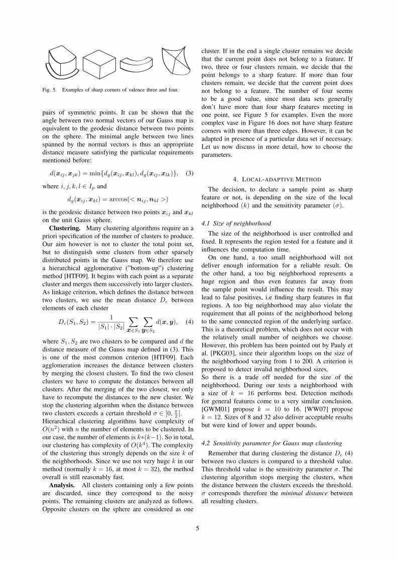
Fig. 5. Examples of sharp corners of valence three and four.

pairs of symmetric points. It can be shown that the

angle between two normal vectors of our Gauss map is

equivalent to the geodesic distance between two points

on the sphere. The minimal angle between two lines

spanned by the normal vectors is thus an appropriate

distance measure satisfying the particular requirements

mentioned before:

d(xij ,xjk) = min{dg(xij ,xkl), dg(xij ,xlk)}, (3)

where i, j, k, l ∈ Ip and

dg(xij ,xkl) = arccos(< nij ,nkl >)

is the geodesic distance between two points xij and xkl

on the unit Gauss sphere.

Clustering. Many clustering algorithms require an a

priori specification of the number of clusters to produce.

Our aim however is not to cluster the total point set,

but to distinguish some clusters from other sparsely

distributed points in the Gauss map. We therefore use

a hierarchical agglomerative (”bottom-up”) clustering

method [HTF09]. It begins with each point as a separate

cluster and merges them successively into larger clusters.

As linkage criterion, which defines the distance between

two clusters, we use the mean distance Dc between

elements of each cluster

Dc(S1, S2) =1

|S1| · |S2|

∑

x∈S1

∑

y∈S2

d(x,y), (4)

where S1, S2 are two clusters to be compared and d the

distance measure of the Gauss map defined in (3). This

is one of the most common criterion [HTF09]. Each

agglomeration increases the distance between clusters

by merging the closest clusters. To find the two closest

clusters we have to compute the distances between all

clusters. After the merging of the two closest, we only

have to recompute the distances to the new cluster. We

stop the clustering algorithm when the distance between

two clusters exceeds a certain threshold σ ∈ [0, π2].

Hierarchical clustering algorithms have complexity of

O(n2) with n the number of elements to be clustered. In

our case, the number of elements is k∗(k−1). So in total,

our clustering has complexity of O(k4). The complexity

of the clustering thus strongly depends on the size k of

the neighborhoods. Since we use not very huge k in our

method (normally k = 16, at most k = 32), the method

overall is still reasonably fast.

Analysis. All clusters containing only a few points

are discarded, since they correspond to the noisy

points. The remaining clusters are analyzed as follows.

Opposite clusters on the sphere are considered as one

cluster. If in the end a single cluster remains we decide

that the current point does not belong to a feature. If

two, three or four clusters remain, we decide that the

point belongs to a sharp feature. If more than four

clusters remain, we decide that the current point does

not belong to a feature. The number of four seems

to be a good value, since most data sets generally

don’t have more than four sharp features meeting in

one point, see Figure 5 for examples. Even the more

complex vase in Figure 16 does not have sharp feature

corners with more than three edges. However, it can be

adapted in presence of a particular data set if necessary.

Let us now discuss in more detail, how to choose the

parameters.

4. LOCAL-ADAPTIVE METHOD

The decision, to declare a sample point as sharp

feature or not, is depending on the size of the local

neighborhood (k) and the sensitivity parameter (σ).

4.1 Size of neighborhood

The size of the neighborhood is user controlled and

fixed. It represents the region tested for a feature and it

influences the computation time.

On one hand, a too small neighborhood will not

deliver enough information for a reliable result. On

the other hand, a too big neighborhood represents a

huge region and thus even features far away from

the sample point would influence the result. This may

lead to false positives, i.e finding sharp features in flat

regions. A too big neighborhood may also violate the

requirement that all points of the neighborhood belong

to the same connected region of the underlying surface.

This is a theoretical problem, which does not occur with

the relatively small number of neighbors we choose.

However, this problem has been pointed out by Pauly et

al. [PKG03], since their algorithm loops on the size of

the neighborhood varying from 1 to 200. A criterion is

proposed to detect invalid neighborhood sizes.

So there is a trade off needed for the size of the

neighborhood. During our tests a neighborhood with

a size of k = 16 performs best. Detection methods

for general features come to a very similar conclusion.

[GWM01] propose k = 10 to 16. [WW07] propose

k = 12. Sizes of 8 and 32 also deliver acceptable results

but were kind of lower and upper bounds.

4.2 Sensitivity parameter for Gauss map clustering

Remember that during clustering the distance Dc (4)

between two clusters is compared to a threshold value.

This threshold value is the sensitivity parameter σ. The

clustering algorithm stops merging the clusters, when

the distance between the clusters exceeds the threshold.

σ corresponds therefore the minimal distance between

all resulting clusters.

5

Fig. 6. Feature detection with a global sensitivity value σ. The points are sampled on a piecewise bilinear surface with a sharp feature line,similar to the example in Fig.7-left. The angle between the surfaces varies along the feature line from acute (45◦) to obtuse (140◦). Thedetected feature points are highlighted by fat red points. σ = 0.05, 0.1, 0.6, 1.0 left to right.

Let us explain the role of this parameter by first

recalling the two main requirements to our method:

1) detection of all points lying on a sharp feature

2) no selection of points which are close to the

feature, but not on it.

These requirements will lead our method to detect a

relatively sparse set of points lying on the sharp feature

or very close to it. Note that the second requirement

is particular to our method, since in most cases, a

sharp feature corresponds to a line. All previous meth-

ods are different in the sense that they aim to detect

general features (not sharp features). Such a feature

often corresponds to surface region with high curvature

variation. Consequently, they compute many points on

the feature followed by a post-processing step, which

reduces the number of points and which replaces them

by an approximating line [GWM01], [PKG03].

The value fixed for the parameter σ ∈ [0, π2] makes

the method more or less sensitive for sharp feature

detection. The sensitivity is inverse reciprocal to the

value of σ. Let us first investigate theoretically how

the method is expected to behave for big and small

sensitivity values, before studying a numerical example:

A big value of σ corresponds to clusters with a big

distance between them obviously implies that clusters

would consist of many points. This would work well

for features which are distinguishly very sharp, i.e.

features with a right angle or an acute angle. But at

the same time it would ignore features with an obtuse

angle. In this case it is more difficult to distinguish the

noisy points from the correct surface normals. If σ is

too big, one would end with only one cluster containing

all points of the Gauss map and the sample point would

not be recognizes as a feature, violating requirement 1.

A small value of σ stops clustering earlier. It would

result in clusters which are more close together

corresponding to feature with an obtuse or an acute

angle. One one hand the method becomes thus more

sensitive for detection of critical sharp features. On the

other hand it may then be difficult to distinguish feature

points from neighbor points, since their clustering

behavior is very similar. It would violate requirement 2.

It seems that there might be some critical features

which are difficult to detect. In practice, the choice of a

Fig. 7. Some examples of sharp feature profiles with varying angles.

user-controlled global sensitivity parameter works well

for many examples. But for more complex examples,

a global sensitivity parameter does not show optimal

results in presence of acute and flat angles in the same

data set. We already suspected this behavior in the

previous paragraph, so let us study now the limits of

the present method with a particular numerical example.

We constructed a piecewise bilinear surface with a

straight feature line where the angle between the surface

varies from acute (45◦) to obtuse (140◦). This data

set corresponds to the left example in Figure 7. In

Figure 6 is shown the result of feature detection for

σ = 0.05, 0.1, 0.6, 1.0. It can be observed, that a very

small value of σ = 0.05 or 0.1 produces many overrates

not only near acute features, i.e. points which are falsely

detected. A mean value of 0.6 detects all features but still

produces overrates near acute features. A big value of

σ = 1.0 however fails to detect flat feature points.

Obviously, if the point cloud contains features with

acute angles and features with obtuse angles, one global

parameter for sensitivity is not sufficient. A good global

value for obtuse angles allows to detect all features,

but will probably overrate features in regions of acute

angles. In this case a whole region might get marked

as sharp feature while the exact position of the feature

cannot be determined. So a global value always needs

a trade-off between finding all features (requirement 1)

and finding the exact position of the features (require-

ment 2).

This observation motivated us to develop an extension

of the algorithm which is presented in the next section.

4.3 Adaptive and local sensitivity parameter

In the previous section it has been demonstrated, that

the use of a global sensitivity parameter σ might not be

sufficient in all cases. In the present section we will show

how to make the parameter σ local and adaptive. The

aim is to develop a method that changes the sensitivity

6

Fig. 8. The two pictures on the left show a non-uniformly sampled point cloud with an overrated set of feature points obtained with twodifferent parameter settings σ = 0.1, k = 20 (left), σ = 0.5, k = 16 (middle). The right figure is the result obtained with the iterative methodapplied to the overrated examples. σ and k are automatically adapted for each of the feature candidates.

value adaptively for different regions of the point cloud.

It should compute automatically an optimal σ value for

each feature candidate. Furthermore we also adapt the

neighborhood size k automatically, so that the user is no

longer obliged to adjust the two parameters manually in

order to get good results.

We achieve this by an iterative process. In a first initial-

ization step the method described in Section 3 including

flatness test on the whole point set and Gauss map

clustering on the selected points does a feature search

using global values for σ and k. In this first passage,

σ will be set to a relatively low value while k will

be relatively large. This delivers a set of many feature

candidates. We generate a larger set in order to not miss

any feature points with an obtuse angle, at the cost of

also getting overrated acute angle features (see Figure 8).

Since we now have a candidate list with many outliers,

we reduce the number of candidates in the following

iteration steps. In these steps the method checks the

number of possible features in the neighborhoods of the

feature candidates.

In the case of a sharp feature e.g. an edge or a curved

line, the feature points will lie on a line dividing the

neighborhood in two parts. The percentage of feature

candidates inside this neighborhood will be relatively

low. A very high percentage of feature candidates inside

a neighborhood indicates that the sensitivity was too

high, i.e. value of σ too low, for this neighborhood. The

existence of only one or no other feature candidate in

the neighborhood indicates that the candidate is not a

sharp feature but an outlier. Thus increasing carefully the

sensitivity value σ would reduce the number of overrated

points, see Figures 6, and 10. To also get rid of the

overrated features at acute angles which don’t disappear

with increasing σ, we also locally reduce the size of the

neighborhoods at every iteration step.

The algorithm for each iteration step is the following.

We raise σ by 10% in the neighborhood of the current

candidate and reduce the neighborhood size k by one.

Then only the candidate features inside this

neighborhood are tested again for being a sharp feature

using the Gauss map clustering described above. The

raised sensitivity and the smaller neighborhood size

lead to a reduction of the number of candidates in this

neighborhood.

This step iterates until either the percentage of features

in the neighborhood of the candidate reaches a

reasonable value (during our experiments a value of

30% of neighborhood size worked well) or another

break condition is reached. These additional breaking

conditions can be chosen among maximum value

for the sensitivity (σ = 1.2), a minimal size for the

neighborhood (k = 8) and a maximum number of

iteration steps.

The iteration process in pseudocode:

while ( iteration break criteria not reached ) {for ( Candidate in Feature Candidates ) {initParameters( n, sigma )Neighborhood = Candidate.Neighborhood

while (Neighborhood.getNumberOfFeatureCandidates()≥ threshold ) {

adjustParameters( n, sigma )

//Check CandidateisFeature=checkforFeature( Candidate, n, sigma )

if ( isFeature == false )removeFromCandidateList( Candidate )

// Check Neighborhood of Candidatefor ( Neighbor ∈ Neighborhood )if ( Neighbor.isFeature() ) {isFeature=checkforFeature( Neighbor, n, sigma )

if ( isFeature == false )removeFromCandidateList( Neighbor )

}}}

}

The right picture in Figure 8 is the result obtained

with the iterative method applied to the overrated

7

examples. σ and k are automatically adapted for each

of the feature candidates. The two pictures on the left

show a point cloud with an overrated set of feature

points obtained with two different parameter settings

σ = 0.1, k = 20 (left), and σ = 0.5, k = 16 (middle).

Adding iterative refinement steps to a process often

increases significantly computational costs. Especially

regarding large point clouds, checking the neighborhood

of every data point iteratively is very costly, O(Nk) in

the worst case where each point has been selected as a

feature candidate. This scenario is of course unrealistic.

In the present setting, the additional computational

costs resulting from the iteration steps are quite low for

two reasons. First, the number of data points checked

during the first iteration is negligible with respect to the

initial data set. They correspond to the feature candi-

dates selected after the first pass using the Gauss map

clustering with a set of not optimal global parameters.

In the case of the ”cube with hole” examples, they

present only 11% of the point cloud. In the case of

the cube without the corner, they present 9%. Second,

the number of remaining feature candidates decreases

significantly after each iteration. This results from the

fact, that each iteration of a single neighborhood will

also eliminate a whole group of other candidates inside

this neighborhood, since the neighborhoods of close

points intersect each other. That means that the neigh-

bors of the candidate, in case of a being not a sharp

feature, are likely to be eliminated from the candidate

list before their their own neighborhood has been tested.

This reduces the number of candidates very fast and

fewer neighborhoods in the cloud will be tested again.

In a usual scenario after the first step only a small

percentage around 10% or less of the point cloud will

be marked as candidate for a sharp feature. This makes

the additional computational costs for the refinement

iterations significantly lower than the costs for the first

global feature search.

5. RESULTS

We have implemented the sharp feature detection

pipeline described in the previous sections. We use both

points sets sampled from some known geometries, such

as the cubes and the bilinear surfaces, as well as more

complex models, such as the ”fandisk” the ”vase”, and

the ”trim-star”. To all models we applied both the basic

algorithm described in Section 3 where we tried to

find some optimal global parameters by testing many

combinations, and the improved local-adaptive method

with an automatic and adaptive choice of the optimal

local parameters. The robustness of the method is tested

and evaluated with respect to two aspects: the variation

of the angle of a sharp feature and noise.

Robustness w/r to varying angles

Let us first test the robustness of the method with

Fig. 9. Feature detection on different angles using the local adaptivemethod.

regard to very acute and obtuse angles by testing two

planes connected with a fixed angle between them.

The profiles of these surfaces are shown in Figure

9. ¿From left to right the angles are 25◦, 45◦, 60◦,

90◦, 110◦, 140◦, 160◦ and 170◦. The method works

perfectly for all angles greater then 45◦, even very

obtuse angles don’t cause any problem. The method

also allows angles of 45◦ and less, but with very acute

angles the results are no longer very precise. In this

case, the overrated points don’t disappear even when

increasing σ and decreasing k. For the three acute

angles the neighborhood was k = 8 for all others we

chose k = 10. The problem of not detected features

appears only with very obtuse angles near 180◦, which

is negligible.

Comparison between global and local-adaptive

method

We then compare the performance of both methods

(global and local-adaptive) using three test examples

with a known number of sharp feature points. The first

example is a simple cube with 580 sharp feature points.

The second example is a surface containing a sharp edge

with a varying angle having 256 sharp feature points.

At one end the angle is (45◦) at the other end it is

(140◦). The third example is cube with a hole with 1350

sharp feature points. We checked the global method with

different sets of parameters and compare it to the local-

adaptive method.

Global method

Figure 10 shows the results for the global method. For

each example 9 sets of parameters have been tested.

The three lines correspond to k = 10, 16, 20, the three

columns correspond to σ = 0.1, 0.5, 0.8.

The simple cube example shows, that for a dataset

with only one kind of angle it is possible to find good

global values for σ and k. k = 10 gives best results,

see Figure 10 (first line). The optimal value of σ = 0.6was found by trying several times the algorithm. It

not fits into the figure here, but it results in a perfect

feature detection of all 256 points of the cube.

In the example of two surfaces joining with the varying

angle, one can see the problems of the global method.

A global value of σ is not sufficient. On one hand, the

feature points on the right part of the edge, where the

angle become obtuse, are not detected when σ = 0.8is big (right column) in Figure 10. On the other hand,

8

Fig. 10. the examples used for the study with the global method.For each example 9 sets of parameters have been tested. The threelines correspond to k = 10, 16, 20, the three columns correspond toσ = 0.1, 0.5, 0.8.

a small σ can detect them, but leads to outliers and

overrates in acute angle regions1. The size of the

neighborhood k has a huge influence on the method

too.

The importance of k is best seen in the cube-with-hole

1The pdf file allows a zoom-in, in order to see all Figures withmore precision.

example. On one hand, a small neighborhood k = 10performs best on the outside edges of the cube, but

leads to bad results in the curved region inside the

hole. On the other hand, a big neighborhood k = 20performs better in the curved areas, but worse on the

outside edges of the cube.

All these examples confirm the conclusion we already

did in Section 3: a global choice of the parameters can

not detect all features satisfactory.

Local-adaptive method

The local-adaptive method can take a huge advantage on

its capability to vary σ and k. For each feature candidate

detected in a first pass, an optimal value of σ and kis determined and outliers are eliminated. However, the

method is not able to add feature points during the

iterations, since the final set of detected features is a

subset of the feature candidates. Therefore, one has to

initialize the iteration with a set of parameters, which

won’t neglect possible features. The experiences in the

previous paragraph show that σ = 0.1 and k = 20 are

good initial values. The result of feature point detection

using the local-adaptive method is shown in Figure 11.

Table 1 resumes the performance of the algorithm with

respect to the three hand-made examples.

Fig. 11. feature detection using the local-adaptive method.

feature# points points detected % outliers

cube 10250 580 575 99%

planes 6090 256 257 100% 1

hole 58720 1350 1398 100% 48

TABLE 1TEST RESULTS FOR THE LOCAL-ADAPTIVE METHOD.

Robustness to noise

In order to test and quantify the sensitivity of our

local adaptive method to noise, we compare distances

measured between real feature points on a test point

cloud and on a perturbed point cloud. The test example

is the cube-with-hole, since it has corner, convex

and concave feature points. All points are lying in a

ball of radius R = 8.5. The original point cloud has

17400 uniformly sampled points. Distance between

neighboring points is 0.25. The perturbed point cloud

is obtained by adding to each point a random vector

chosen in a ball whose size is 0.4%, 0.8% and 1.2% of

R.

The error induced by the noise is measured using the

distances between the set of feature points in the original

9

Noise δ∞ δavg # features

0.0 % 0 0 839 (+0)

0.4 % 0.25 0.02 862 (+23)

0.8 % 0.26 0.03 875 (+36)

1.2 % 0.31 0.08 984 (+145)

1.6 % 0.75 0.19 1245 (+406)

2.0 % 0.93 0.21 1255 (+416)

TABLE 2DISTANCES BETWEEN ESTIMATED FEATURES AND REAL FEATURES

OF THE CUBE-WITH-HOLE MODEL. NOISE AS A PERCENT OF THE

MODEL RADIUS VARIES. THE NUMBER OF EXACT FEATURES 839 IS

COMPARED TO THE NUMBER OF ESTIMATED FEATURES.

point cloud Q = {qi} and the set of estimated feature

points in the perturbed point cloud P = {pi}. The

distances δ∞ and δavg are defined similar to [MOG09].

δ∞ is the maximal distance between an estimated feature

point pi and its nearest feature point in Q. δavg is the

average distance between an estimated feature point pi

and its nearest neighbor in Q.

Table 2 summarizes the results of the experiment for

different noise radii. The number of detected feature

points is also a measure of quality, since our method

aims to detect only feature points or a sparse set of

points very close to a feature,

δ∞ measures the presence of outliers. The experiment

shows that in the case of mean noise (0.8%) the distance

of isolated outliers δ∞ = 0.26 is equal to the point

distance (0.25) in the original point cloud. Outliers are

thus very close the neighbors of real features, see Figure

12. For bigger noise of 1.2% the isolated outliers are

still very close to the feature points, but their number

increases. Even though the number of so-called false

features increases with increasing noise, the detection

method is still stable, since isolated outliers stay close

to real features, even for big noise.

Noise 0.0 % Noise 0.4 % Noise 0.8 %

Noise 1.2 % Noise 1.6 % Noise 2.0 %

Fig. 12. Estimated feature points on noisy point clouds. The originalcube-with-hole model is perturbed with random noise.

Complex point-sampled surfaces

After these self constructed examples let us show some

more real world examples. Here it is not possible

anymore to measure the quality of the output of the

Fig. 13. The global method on the fandisk and the trim-star.

algorithm, since the feature points are not known and

generally don’t ly directly on the feature as stated in

[AFRS05]. Only a visual control is possible. First we

tried the global method on the well-known fandisk

(σ = 0.7, k = 12) and the trim-star (σ = 0.6, k = 12).

It can be seen in Figure 13 that no optimal result

can be achieved. We then applied the local-adaptive

method to the following three examples. Figure 14

shows the detected sharp feature points on the fandisk

model (41250 vertices). The local method here again

delivers good results. The next examples in Figures 15

and Figure 16 show the trim-star model (25100 vertices)

and the vase (896000 vertices) which has some curvy,

sharp features. Notice, that for the vase and the trim-

star, the original model is a triangulation, but the points

are NOT lying on the feature. The triangle edges are

zig-zagging along the feature lines.

Fig. 14. Sharp feature detection on the fandisk model.

Fig. 15. Sharp feature detection on the trim-star model.

Finally we used a scan data set by a CyberwareTM

scanner of a drill. Many data is missing near the sharp

features and the precision is quite rough, see Figure 17,

but the feature lines are correctly detected along the

10

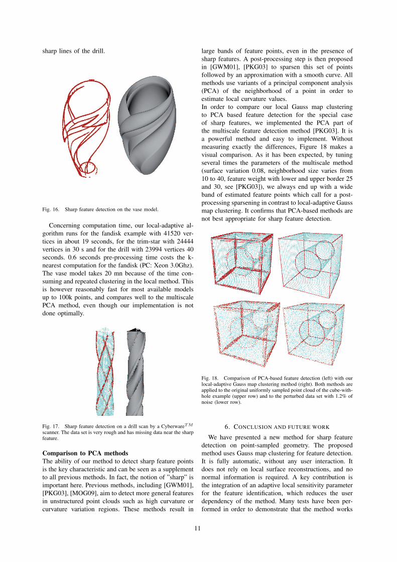
sharp lines of the drill.

Fig. 16. Sharp feature detection on the vase model.

Concerning computation time, our local-adaptive al-

gorithm runs for the fandisk example with 41520 ver-

tices in about 19 seconds, for the trim-star with 24444

vertices in 30 s and for the drill with 23994 vertices 40

seconds. 0.6 seconds pre-processing time costs the k-

nearest computation for the fandisk (PC: Xeon 3.0Ghz).

The vase model takes 20 mn because of the time con-

suming and repeated clustering in the local method. This

is however reasonably fast for most available models

up to 100k points, and compares well to the multiscale

PCA method, even though our implementation is not

done optimally.

Fig. 17. Sharp feature detection on a drill scan by a CyberwareTM

scanner. The data set is very rough and has missing data near the sharpfeature.

Comparison to PCA methods

The ability of our method to detect sharp feature points

is the key characteristic and can be seen as a supplement

to all previous methods. In fact, the notion of ”sharp” is

important here. Previous methods, including [GWM01],

[PKG03], [MOG09], aim to detect more general features

in unstructured point clouds such as high curvature or

curvature variation regions. These methods result in

large bands of feature points, even in the presence of

sharp features. A post-processing step is then proposed

in [GWM01], [PKG03] to sparsen this set of points

followed by an approximation with a smooth curve. All

methods use variants of a principal component analysis

(PCA) of the neighborhood of a point in order to

estimate local curvature values.

In order to compare our local Gauss map clustering

to PCA based feature detection for the special case

of sharp features, we implemented the PCA part of

the multiscale feature detection method [PKG03]. It is

a powerful method and easy to implement. Without

measuring exactly the differences, Figure 18 makes a

visual comparison. As it has been expected, by tuning

several times the parameters of the multiscale method

(surface variation 0.08, neighborhood size varies from

10 to 40, feature weight with lower and upper border 25

and 30, see [PKG03]), we always end up with a wide

band of estimated feature points which call for a post-

processing sparsening in contrast to local-adaptive Gauss

map clustering. It confirms that PCA-based methods are

not best appropriate for sharp feature detection.

Fig. 18. Comparison of PCA-based feature detection (left) with ourlocal-adaptive Gauss map clustering method (right). Both methods areapplied to the original uniformly sampled point cloud of the cube-with-hole example (upper row) and to the perturbed data set with 1.2% ofnoise (lower row).

6. CONCLUSION AND FUTURE WORK

We have presented a new method for sharp feature

detection on point-sampled geometry. The proposed

method uses Gauss map clustering for feature detection.

It is fully automatic, without any user interaction. It

does not rely on local surface reconstructions, and no

normal information is required. A key contribution is

the integration of an adaptive local sensitivity parameter

for the feature identification, which reduces the user

dependency of the method. Many tests have been per-

formed in order to demonstrate that the method works

11

very successfully even on very complex geometry in

contrast to algorithms based on global parameters. The

resulting point cloud with the marked sharp features

can be used for several applications now (surface recon-

struction, non-photorealistic rendering, mesh generation,

MLS-surface modeling). In [GWM01] a hole section

is devoted to possible applications. The properties of

the resulting feature point set (preciseness, sparseness,

very few outliers) make the method an excellent pre-

processing step for feature line approximation with

smooth spline curves [GWM01].

All line-type, corner-type sharp features are detected.

Cone peaks are not treated here, the method needs to be

adapted in order to recognize the particular clustering

behavior in this case.

ACKNOWLEDGMENTS

The vase model is provided courtesy of INRIA, the

fandisk and trim-star are provided courtesy of MPII, all

by the AIM@SHAPE Shape Repository. The drill model

is courtesy of Sergei Azernikov, Siemens Corporate

Research, Princeton.

This work was supported by the IRTG 1131 of the

DFG (German Research Foundation). It has been par-

tially supported by the Deutsche Forschungsgemein-

schaft INST 248/72-1.

REFERENCES

[ACK01] AMENTA N., CHOI S., KOLLURI R. K.: The power crust.In SMA ’01: Proceedings of the sixth ACM symposium on

Solid modeling and applications (New York, NY, USA,2001), ACM, pp. 249–266.

[AFRS05] ATTENE M., FALCIDIENO B., ROSSIGNAC J., SPAGN-UOLO M.: Sharpen&bend: Recovering curved sharp edgesin triangle meshes produced by feature-insensitive sam-pling. IEEE Transactions on Visualization and Computer

Graphics 11, 2 (2005), 181–192.

[AGJ00] ADAMY U., GIESEN J., JOHN M.: New techniques fortopologically correct surface reconstruction. In VISUAL-

IZATION ’00: Proceedings of the 11th IEEE Visualization

2000 Conference (VIS 2000) (Washington, DC, USA,2000), IEEE Computer Society.

[AMN∗98] ARYA S., MOUNT D. M., NETANYAHU N. S., SIL-VERMAN R., WU A. Y.: An optimal algorithm forapproximate nearest neighbor searching fixed dimensions.J. ACM 45, 6 (1998), 891–923.

[BL97] BEIS J. S., LOWE D. G.: Shape indexing using ap-proximate nearest-neighbour search in high-dimensionalspaces. In CVPR ’97: Proceedings of the 1997 Conference

on Computer Vision and Pattern Recognition (CVPR ’97)

(Washington, DC, USA, 1997), IEEE Computer Society,p. 1000.

[CLR01] CORMEN T. H., LEISERSON C. E., RIVEST R. L.: Intro-

duction to Algorithms, 2th ed. MIT Press and McGraw-Hill, Boston, MA, USA, 2001.

[DOHS08] DANIELS J., OCHOTTA T., HA L. K., SILVA C. T.:Spline-based feature curves from point-sampled geometry.Vis. Comput. 24, 6 (2008), 449–462.

[DVVR07] DEMARSIN K., VANDERSTRAETEN D., VOLODINE T.,ROOSE D.: Detection of closed sharp edges in pointclouds using normal estimation and graph theory. Comput.

Aided Des. 39, 4 (2007), 276–283.

[FCOS05] FLEISCHMANN S., COHEN-OR D., SILVA C.: Robustmoving least-squares fitting with sharp features. ACM

Trans. Graph. (2005), 37–49.

[GM97] GUY G., MEDIONI G.: Inference of surfaces, 3d curves,and junctions from sparse, noisy,3d data. IEEE Transac-

tions on Pattern Analysis and Machine Intelligence 19,11 (1997), 1265–1277.

[GWM01] GUMHOLD S., WANG X., MCLEOD R.: Feature extrac-tion from point clouds. Proceedings of 10th International

Meshing Roundtable (2001).[HDD∗92] HOPPE H., DEROSE T., DUCHAMP T., MCDONALD J.,

STUETZLE W.: Surface reconstruction from unorganizedpoints. In SIGGRAPH ’92: Proceedings of the 19th

annual conference on Computer graphics and interactive

techniques (New York, NY, USA, 1992), ACM, pp. 71–78.

[HG01] HUBELI A., GROSS M.: Multiresolution feature ex-traction for unstructured meshes. Proccedings of IEEE

Visualization (2001), 287–294.[HPW05] HILDEBRAND K., POLTHIER K., WARDETZKY M.:

Smooth feature lines on surface meshes. Proceedings of

Symposium on Geometric Processing (2005).[HTF09] HASTIE T., TIBSHIRANI R., FRIEDMAN J.: The Elements

of Statistical Learning: Data Mining, Inference, and Pre-

diction., 2th ed. Springer, Boston, MA, USA, 2009.[JPR00] JUNGHYUN H., PRATT M., REGLI W.: Manufacturing

feature recognition from solid models: a status report.IEEE Transactions on Robotics and Automation 16, 6(2000), 782–796.

[KBSS01] KOBBELT L., BOTSCH M., SCHWANECKE U., SEIDEL

H.-P.: Feature sensitive surface extraction from volumedata. In SIGGRAPH ’01: Proceedings of the 28th annual

conference on Computer graphics and interactive tech-

niques (New York, NY, USA, 2001), ACM, pp. 57–66.[LW77] LEE D., WONG C.: Worst-case analysis for region and

partial region searches in multidimensional binary searchtrees and balanced quad trees. Acta Informatica 9 (1977).

[LX08] LIU Y., XIONG Y.: Automatic segmentation of unor-ganized noisy point clouds based on the gaussian map.Comput. Aided Des. 40, 5 (2008), 576–594.

[MOG09] MRIGOT Q., OVSJANIKOV M., GUIBAS L. J.: Ro-bust voronoi-based curvature and feature estimation. InSymposium on Solid and Physical Modeling (2009),Bronsvoort W. F., Gonsor D., Regli W. C., Grandine T. A.,Vandenbrande J. H., Gravesen J., Keyser J., (Eds.), ACM,pp. 1–12.

[OGG09] OZTIRELI C., GUENNEBAUD G., GROSS M.: Featurepreserving point set surfaces based on non-linear kernelregression. Computer Graphics Forum 28, 2 (2009).

[PKG03] PAULY M., KEISER R., GROSS M.: Multi-scale featureextraction on point-sampled surfaces. Computer Graphics

Forum (2003).[WB01] WATANABE K., BELYAEV A. G.: Detection of salient

curvature features on polygonal surfaces. Computer

Graphics Forum (2001), 385–392.[WG09] WEINKAUF T., GNTHER D.: Separatrix persistence:

Extraction of salient edges on surfaces using topologicalmethods. Computer Graphics Forum (Proc. SGP ’09) 28,5 (July 2009), 1519–1528.

[WW07] WU J., WANG Q.: Feature point detection from pointcloud based on repeatability rate and local entropy. InProceedings of the SPIE Vol.6786 (2007), p. 67865.

12