Embed Size (px)
Citation preview
SHARED CONTROL FOR TELEOPERATION
USING A LIE GROUP APPROACH
Brian Hunter
Submitted in part fulfilment of the requirements for the Degree of Doctor of Philosophy of the University of London
1996

ProQuest Number: 10045734
All rights reserved
INFORMATION TO ALL USERS The quality of this reproduction is dependent upon the quality of the copy submitted.
In the unlikely event that the author did not send a complete manuscript and there are missing pages, these will be noted. Also, if material had to be removed,
a note will indicate the deletion.
uest.
ProQuest 10045734
Published by ProQuest LLC(2016). Copyright of the Dissertation is held by the Author.
All rights reserved.This work is protected against unauthorized copying under Title 17, United States Code.
Microform Edition © ProQuest LLC.
ProQuest LLC 789 East Eisenhower Parkway
P.O. Box 1346 Ann Arbor, Ml 48106-1346
SHARED CONTROL FOR TELEOPERATION
USING A LIE GROUP APPROACH
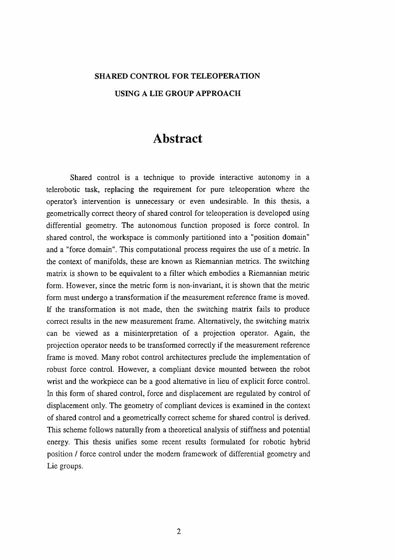
Abstract
Shared control is a technique to provide interactive autonomy in a
telerobotic task, replacing the requirement for pure teleoperation where the
operator’s intervention is unnecessary or even undesirable. In this thesis, a
geometrically correct theory of shared control for teleoperation is developed using
differential geometry. The autonomous function proposed is force control. In
shared control, the workspace is commonly partitioned into a "position domain"
and a "force domain". This computational process requires the use of a metric. In
the context of manifolds, these are known as Riemannian metrics. The switching
matrix is shown to be equivalent to a filter which embodies a Riemannian metric
form. However, since the metric form is non-invariant, it is shown that the metric
form must undergo a transformation if the measurement reference frame is moved.
If the transformation is not made, then the switching matrix fails to produce
correct results in the new measurement frame. Alternatively, the switching matrix
can be viewed as a misinterpretation of a projection operator. Again, the
projection operator needs to be transformed correctly if the measurement reference
frame is moved. Many robot control architectures preclude the implementation of
robust force control. However, a compliant device mounted between the robot
wrist and the workpiece can be a good alternative in lieu of explicit force control.
In this form of shared control, force and displacement are regulated by control of
displacement only. The geometry of compliant devices is examined in the context
of shared control and a geometrically correct scheme for shared control is derived.
This scheme follows naturally from a theoretical analysis of stiffness and potential
energy. This thesis unifies some recent results formulated for robotic hybrid
position / force control under the modem framework of differential geometry and
Lie groups.
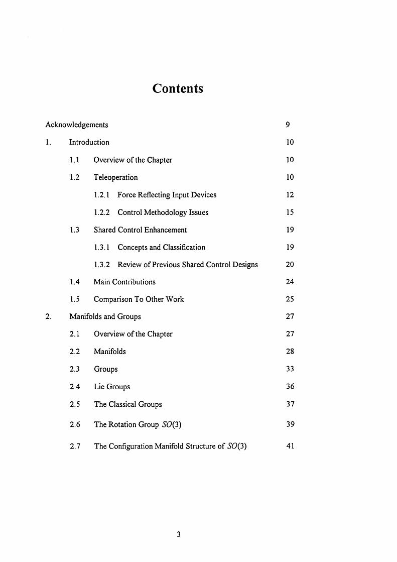
Contents
Acknowledgements 9
1. Introduction 10
1.1 Overview o f the Chapter 10
1.2 Teleoperation 10
1.2.1 Force Reflecting Input Devices 12
1.2.2 Control Methodology Issues 15
1.3 Shared Control Enhancement 19
1.3.1 Concepts and Classification 19
1.3.2 Review o f Previous Shared Control Designs 20
1.4 Main Contributions 24
1.5 Comparison To Other W ork 25
2. Manifolds and Groups 27
2.1 Overview o f the Chapter 27
2.2 Manifolds 28
2.3 Groups 33
2.4 Lie Groups 36
2.5 The Classical Groups 37
2.6 The Rotation Group S0{3) 39
2.7 The Configuration Manifold Structure o f S0{3) 41
Contents (continued)
3. Calculus on Manifolds 43
3.1 Overview o f the Chapter 43
3.2 Tangent Vector 43
3.3 Infinitesimal Operator 47
3.4 Infinitesimal Operator o f 7(3) 49
3.5 Infinitesimal Operator o f ^(9(3) 50
3.6 Commutation Relations 54
3.7 Lie Algebra 56
3.7.1 Lie Subalgebras 57
3.7.2 Ideals 58
3.7.3 Simple and Semisimple Lie Algebras 58
3.7.4 Solveable Lie Algebras 60
3.7.5 Direct and Semidirect Sums 61
3.7.6 Classification o f 5e(3) 61
3.8 Infinitesimal Generators 62
3.9 Induced Maps on Manifolds 63
4. Representation o f the Lie Algebra o f the Special Euclidean Group 65
4.1 Overview o f the Chapter 65
4.2 M atrix Representation o f 5^(3) 65
Contents (continued)
4.3 Differential M ap 69
4.4 Differential M ap on a Moving Reference Frame 73
4.5 Lie Bracket 75
4.6 Exponential Map 76
4.7 The Product o f Exponentials Formula 80
5. Riemannian Metrics 85
5.1 Overview o f the Chapter 85
5.2 Dual Vector 85
5.3 Riemannian Metric 87
5.4 Isometry 89
5.5 A , - Invariant Riemannian Metric 91
5.6 Kinetic Energy Metric 98
5.7 Orthogonality and Reciprocity 100
5.8 Validation o f the Reciprocal Product 101
6. Invariant Filtering for Shared Control 103
6.1 Overview o f the Chapter 103
6.2 Partitioning o f Vector Spaces 104
6.3 Left Pseudo-Inverse 107
6.4 Conceptual Design for a Shared Controller 110
6.5 Design for Invariant Filtering 112
6.6 Shared Control and Constrained M otion 112
Contents (continued)
6.7 Symplectic V ector Space 114
6.8 Constraints 117
6.9 Conceptual Scheme for Constrained M otion 120
6.10 Validation o f Invariant Filtering 121
6.11 Projection Operators 125
6.12 Transformation o f Velocity 128
7. Compliance and Shared Control 130
7.1 Overview o f the Chapter 130
7.2 Stiffness 131
7.3 Potential Energy 132
7.4 Conceptual Scheme for Shared Control 134
8. Conclusions 139
8.1 Overview o f the Chapter 139
8.2 Contributions o f the Thesis 139
8.3 Ideas for Future Research 140
References 142
A l.l Switching Matrix Test Harness 150
A1.2 Invariant Filter Test Hames 156
A1.3 Test Harness for Projection Operator 162
A1.4 Test Harness for Generalized Spring 168
A2 Mathematical Proofs 172
List of Figures
1-1 Peg Insertion Task 22
2-1 Differential M anifold 30
2-2 Coordinate Function 31
2-3 Configuration Manifold for SE{3) 37
3-1 Open Curve 44
3-2 Function 45
3-3 Tangent Vector 46
3-4 Infinitesimal Operator 47
3-5 Induced Map on Manifolds 64
4-1 Active Transformation 69
4-2 Passive Transformation 72
4-3 Moving Reference Frame 73
4-4 Integral Curve 77
4-5 Mapping from Joint Space to SE(3) 80
4-6 Joint Space Manifold for a 2R Planar Robot 81
6-1 Partition of the Tangent Space 104
6-2 Conceptual Design for Shared Control 110
6-3 Partially Constrained Rigid Body 117
6-4 Conceptual Shared Control Scheme 120
6-5 Shared Control Task with Displaced Reference Frame 122
List of Figures (continued)
7-1 Conceptual Shared Control Scheme 134
7-2 Generalized Spring 135
7-3 Generalized Spring with Shifted Reference Frame 137
List of Tables
3-1 Commutation Relations 55
"and fo r the sake o f all things in general let us recall to mind
that nothing can be known concerning the things o f this world
without the pow er o f geometry . . ."
Roger Bacon
Acknowledgements
This thesis was undertaken with the support of Telerobotic Systems, AEA
Technology. I would like to thank C.J.H. Watson and M.H. Brown for giving their
support to my registration at University College London.
I am very grateful to my supervisors - David Broome of UCL and Siva of
AEA - and wish to thank them for giving me the freedom to explore ideas under
their guidance and for their patience.
I would like to thank Patrick Fischer, Paul Elosegui, Ross McAree and
Ron Daniel for many fruitful technical discussions over the years. I am indebted to
Dr. J.M. Selig of Southbank University, Dr. J. Gilby of Sira Ltd and Dr. A. Greig
of UCL for their critical review of my work.
M ost of all I would like to thank my wife, Anne-Marie, and my parents.
Bill and Jean, for their emotional support and for their belief in me, without which
this thesis would surely not have been completed.
Chapter 1
Introduction
1.1 Overview of the Chapter
In this chapter, some basic concepts behind teleoperation and shared
control are explained. A review of previous work on the implementation of shared
control is also presented. Finally, the main contributions of this dissertation are put
forward.
1.2 Teleoperation
The term "teleoperation" is used to describe mechanical activities
performed by mechanical devices at a remote site under remote control. The
remotely performed mechanical actions are usually associated with the normal
work function of the human arm and hand. Thus teleoperation extends the
manipulative capabilities of the human arm and hand to remote, physically
difficult, or dangerous environments (Bejczy 1980a).
10
The first teleoperator systems were developed in the 1940s to allow an
operator to handle radioactive materials from a workroom separated from the
radioactive environment by a concrete wall. The operator observed the work scene
through viewing ports in the wall. The development of teleoperator devices for
handling radioactive materials culminated in the introduction of bilateral master-
slave manipulator systems. In these very successful systems, the slave arm at the
remote site is mechanically or electrically coupled to the geometrically identical or
similar master arm and thus follows the motion of the master arm. But the
coupling between the master and slave arms is two-way: inertial or external forces
on the slave arm can backdrive the master arm. Hence the operator holding the
master arm can feel forces acting on the slave arm. This is an essential
requirement for dextrous control of remote manipulators, since general purpose
manipulation consists of a series of well-controlled contacts or "collisions"
between the handling device and the objects (Bejczy 1980a).
Master-slave teleoperator technology has been expanding to accommodate
new telemanipulation requirements in space, under the sea, in nuclear facilities,
and in other frontiers of science. This is reflected in a NASA study that described
a teleoperator as
" a robotic device having video and/or other sensors, manipulator arms, and some
mobility’ capability, which is remotely controlled over a telecommunication
channel by a human operator. This human operator can be a direct in-the-loop
controller who observes a video display o f the teleoperator and, with joystick or
analog device, continuously controls the position o f the teleoperator vehicle, its
arm, or its sensor orientation. Alternatively, the teleoperator can employ a
computer, endowed with a modicum o f artificial intelligence, capable o f executing
simple control functions automatically through local force or proximity sensing:
in this case, the remote human operator shares and trades control with the
computer" (Bejczy 1980a)
11
The bilateral force reflecting master-slave manipulator is a successful
example of where a kinaesthetic coupling between operator and remote
manipulator has been established. However, the establishment of this type of
coupling is not constrained to geometrically similar master-slave systems; it is
possible to establish a kinaesthetic coupling via a "universal" force reflecting input
device - in fact, this can be viewed as a generalization of the technique (Bejczy
1980b).
1.2.1 Force-Reflecting Input Devices
The force-reflecting input device serves a general purpose in that it does
not have any geometric or kinematic correspondence with the mechanical arm it
controls and from which it is backdriven. The position control relation between
this device and a mechanical arm is established through real-time mathematical
transformation of Joint variables measured at both the input device and the
mechanical arm. Likewise, the forces and torques sensed at the base of the end
effector are resolved into appropriate input device joint drives through real-time
mathematical transformations to give the operator’s hand the same force-torque
"feeling" that is felt by the end effector on the remote mechanical arm (Bejczy
1980a).
An outline specification for a high fidelity force-reflecting input device
was first proposed by Goertz (1964). Although his work was aimed primarily at
conventional master-slave manipulator systems, the specification is consistent
with aspects of more recent specifications devised for modem force-reflecting
input devices. He noted that the master-slave systems had the same frequency
response in both the directions but that this was inconsistent with the capabilities
of the human operator; the human motor system was capable of generating
12
frequencies of around lOHz but the nervous system could detect much higher
transient frequencies through the hand. Goertz (1964) proposed that a manipulator
that was more consistent with the operator’s capabilities might require a bandwidth
of between lOOHz to IkHz .
The issue of input device specification was raised more recently by
McAffee and Fiorini (1991) and Fischer et al (1990). These specifications arose
from an attempt to formalize the design of desk-top input devices that were
kinematically dissimilar from the slave arms that they were controlling. These new
devices have potential for excellent performance compared to conventional
master-slave manipulators, especially where space constraints exist, since they are
kinematically optimized for the human operator interface and not matched to the
slave.
Development work undertaken at the Jet Propulsion Laboratory (JPL)
raised many of the important issues associated with the design and control of desk
top force-reflecting input devices. The JPL Force Reflecting Hand Controller
(FRHC) was under development for much of the early 1980s (Bejczy and
Handlykken 1981) culminating in a flight prototype version at the end of the
decade (McAffee et al 1990). More recently, AEA have produced an input device
based on the Stewart Platform geometry, the Bilateral Stewart Platform (BSP)
(Fischer 1993).
13
McAffee and Fiorini (1991) gives a summary of a suitable specification for a
force-reflecting input device as follows:
"Highly intuitive operation:
provides fu ll 6-dof articulation to specify a unique spatial position and
orientation,
provides excellent kinaesthetic feedback to the human operator to produce
the same physiological motor sensations as i f performing the task in
person,
configures the remote reference fram e so that it coincides with the
operators own body reference,
assures that spatial transformations are transparent to the operator,
inakes use o f human eye-hand co-ordination so that commands can be
given almost instinctively by the operator,
allows a shorter learning time.
Universal (generalized) applicability’:
provides a common interface to control dissimilar remote systems,
accommodates many control modes and allows fo r system performance
adjustments.
Good 6-do f position and orientation resolution:
guarantees accurate sensing o f position and orientation commands from
the operator,
assures that the mechanism has a min imum o f backlash.
14
High fidelity force feedback:
faithfully reproduces remote forces and torques,
generates crisp and distinguishable force and torque cues.
Good mechanical design:
provides the mechanical stijfness necessary fo r a large system bandwidth,
provides the simple kinematic structure necessary fo r fa s t kinematic and
dynamic inode Is,
provides mechanically decoupled joints, simplifying control algorithms,
assures good backdrive ability by minimizing friction and inertia fo r higher
force resolution and lower operator fatigue. "
1.2.2 Control Methodology Issues
Typically a force-reflecting input device is not a kinematically similar
mechanism to the manipulator arm that it is controlling and is designed to utilize a
more generalized form of control, the so-called resolved motion control (Whitney
1969). In this case the manipulator motion is specified in terms of a trajectory in
the Cartesian workspace and is conceptually easy for the operator to use.
Resolved motion control is so-named because the required motion in the
Cartesian workspace is resolved into a sequence of six joint angle commands for
the manipulator joint servo drivers. Resolved motion control references the
position and orientation of the manipulator’s gripper, requiring three positions to
fix the position of the gripper in three dimensional space and three rotations to fix
the orientation of the gripper (Whitney 1969).
15
A common approach for resolved motion control is to use two three-axis
joysticks to realize the three position commands and three orientation commands.
However, a six degree of freedom input device integrates the function of two
joysticks into one unit, enabling one-handed operation. The forward kinematic
solution is a function of the input device mechanism design. For example, a
numerical solution is required for the parallel BSP mechanism (Fischer 1993). The
mapping that transforms Cartesian commands to joint commands is the inverse
kinematics of the manipulator. This needs to be calculated at every sampling time.
The design of the robot wrist can greatly simplify the computational burden
associated with solving the inverse kinematics of the arm; the three wrist joint
axes should intersect at a point (Craig 1986)).
Force-reflecting operation can be achieved with position-position control
(Goertz et al 1961). This has the been the classic method for bilateral control,
employed very successfully for master-slave manipulators for many years (Goertz
et al 1966). This control mode is very simple since it involves no direct
measurement of forces (Siva 1985). It is essentially two unilateral position
servomechanisms connected back-to-back and the position error made common to
both servo systems (Raimondi 1976). The position-position servo-system
essentially requires backdriveability between the master and slave servo-drives
(Siva 1992). Therefore, this method (in its basic form) is unsuitable for inherently
non-backdriveable servo-systems. An example is a hydraulic servo-position
system, controlled by a flow controlled servo-valve (Mosher 1960). In this case,
the situation can be remedied by using a special pressure control servo-valve or by
backdriving the master-arm (using a signal derived from the pressure differential
across the actuator) and relying on the closed-loop position control to backdrive
16
the slave (Wilson 1975). It should be noted that friction in either the master or
slave will affect the success of this scheme.
Position-position control can also be employed on dissimilar input devices
by considering position errors in Cartesian space rather than in joint space (Kim
1991). A non-backdriveable servo-system (such as a robot joint-servo using a high
reduction gearbox) can use compliance control in order to achieve
backdriveability. A major advantage here is that the position/orientation command
from the input device can be perturbed directly; the input device itself does not
need to be backdriven. This is because there is no absolute correspondence to
maintain between the input device position and the manipulator position.
Therefore, friction in the input device is irrelevant to the success of the technique.
Force-reflecting operation can be achieved with force-position control
(Handlykken and Turner 1980). This mode of control is configured by essentially
implementing two control loops. The first loop is a position control loop which
serves to send position commands to the robot from an input device. The second
loop is a force control loop which serves to implement force commands to the
input device from the robot. This scheme has been successfully implemented for
master-slave servo systems where a measurement of joint torque is required
(Bicker 1990). Force-position control can also be employed on dissimilar input
devices by considering measurement of forces in Cartesian space rather than in
joint space. A wrist-mounted force sensor is used to measure end-point forces and
torques in the tool coordinate frame. These measurements are then transformed
from the tool coordinate frame to the world coordinate frame using a
transformation matrix derived from the orientation of the manipulator wrist. The
force measurement is then transformed into input device joint space, via the
17
transpose of the input device Jacobean and used to backdrive the input device thus
establishing the kinaesthetic coupling to the operator (Bejczy and Salisbury 1983).
In a typical telemanipulation system, the manipulator is under closed loop
position control. The manipulator is typically stiff and small errors between the
actual and the commanded position can give rise to undesired large contact forces
and torques (Hannaford 1989). The same problem arises with automatic force
control of manipulators and, although many approaches have been tried, the
problem of oscillatory contact with a rigid environment persists (Eppinger and
Steering 1987). Force-position control has been implemented on the JPL FRHC
(Handlykken and Turner 1980). The stability problem meant that force gains had
to be turned down. This meant that the maximum force ratio attainable without
causing instability was only approximately 10:1. This meant that only IN force
could be felt for a ION force on the manipulator (Kim 1991). This is the trade-off
that appears to exists when only a simple force-position loop is implemented.
This situation can be alleviated by adding compliance and damping to the
stiff robot. Active compliance and damping, emulating a programmable
mechanical passive spring and damper for each Cartesian axis, can be
implemented by first low pass filtering the force-torque signal from the wrist-
mounted force sensor and then feeding back the low pass filtered signal to the
position/orientation command signal from the input device. When implemented
into a system incorporating a bilateral input device, the approach is called shared
compliant control (Kim et al 1992). There are two parameters to control:
compliance (or its inverse, stiffness) and damping. The compliance of the active
spring is proportional to the force feedback gain K. The damping of the active
damper is proportional to T/K, where T is the time constant of the first-order low
18
pass filter. If a pure gain is used instead of the low pass filter, a spring with no
damper is realized. If an integrator is used instead of the low pass filter, a damper
with no spring is realized (Kim 1990).
The problem of instability can be reduced by introducing damping into the
system via the input device (Fischer 1993). However, there is a trade-off because
high levels of damping on the input device can be fatiguing for the operator. Other
approaches to combat instability are force signal frequency shaping and digital
compensation (Fischer 1993).
1.3 Shared Control Enhancement
1.3.1 Concepts and Classification
In shared control, control of the six degrees of freedom of the tasks pace is
shared with computer control algorithms referenced to a sensor or to some other
world model information (Bejczy 1980a). Shared control is designed to inject
autonomy into a telerobotic task, replacing the requirement for pure teleoperation
in those situations where the operator’s intervention is unnecessary or even
undesirable.
It is appropriate to produce a rigorous definition and classification of sub-
types. The terminology given in Yoerger and Slotine (1987) is adopted. Two basic
forms of shared control are identified - serial and parallel.
19
In serial form, the control of the manipulator is switched in series between
the operator and the autonomous function. In parallel form, the human operator
and the autonomous function jointly execute the task (Yoerger and Slotine 1987).
The parallel form can be sub-divided further to two forms (Yokokohji et al
1993). These forms are termed combined and non-combined. In the combined
form, the autonomous control is mixed with the operator control. An example is
collision avoidance, where the operator’s command is modified is some way,
perhaps by proximity sensors, to avoid contact. A second example, though more
subtle, is shared compliant control (SCC); again the operators command is
modified by information from a sensor - in this case a force-torque sensor.
In the non-combined form, there is no mixing on any degree of freedom,
but there is a mix of operator and autonomous control across the available degrees
of freedom. If the autonomous control is a force control action, then we have a
form of shared control that is analogous with the classic robotic hybrid position /
force control. (Raibert and Craig 1981). The difference is that position control is
from a human operator rather than from a robot trajectory generator.
1.3.2 Review of Previous Shared Control Designs
Shared control has been implemented on a number of teleoperator systems
for use in space. The ROTEX experiment (Hirzinger et al 1992) was designed to
test a number of concepts involved in the implementation of a partly autonomous
robot system with extensive ground control capabilities for the European Space
Agency. The experiment featured a small, six-axis robot (working volume around
Im^) moving inside a space-lab rack integrated into the US space shuttle. Its
20
gripper was provided with a number of sensors, including a 6-axis force-torque
sensor. The experiment has successfully flown in space on spacelab mission D2 on
shuttle flight STS 55 from April 26 to May 6, 1993 (Hirzinger et al 1993). A
parallel - non-combined form of shared control was used.
Shared control was used in the telerobotics validation experiments and
demonstrations for the Space Station Freedom program (Backes et al 1993). The
Johnson Space Centre in Houston acted as the local ground site and the JPL
Supervisory Telerobotics (STELER) laboratory in Pasadena acted as the remote
site. Operator control stations were supported at both the local ground site and the
remote site, the remote site allowing teleoperation and shared control where time
delays were of an acceptable order. The robot was a Robotics Research K1207 and
the Modular Telerobot Task Execution System (MOTES) provided the remote site
execution capability. The input device was a JPL/Salisbury Model C Hand
Controller (Backes et al 1993). The control of each task space could be shared
between a position control mode (via an input device) and a compliant control
mode -termed as "force nulling" (Bejczy 1988). This form of shared control is
parallel- non-combined. Force control was accomplished with a force control loop
closed around an inner position control loop (Backes 1990). The force nulling
mode was achieved by producing a position setpoint for the selected degree of
freedom based on integration of the sensed force or torque in that direction. Stein
(1993) detailed a more general force mode for the JPL Advanced Teloperation
(ATOP) Laboratory which referenced a setpoint force value. A non-zero setpoint
caused the robot to attempt to maintain a contact force, whilst a zero setpoint
yielded a control action that avoided contact; the latter action is the same as force
nulling. Stein (1993) also added a feature to the system whereby the shared control
could be configured in either the world or the tool frame. The shared control
21
capability was built into high level task primitives that could be selected by the
operator from a menu.
Hayati and Venkataraman (1989) attempted to define a generic shared
system architecture for software implementation. This was based on switching
matrices to segment input vectors in an appropriate fashion. This was similar in
concept to the switching matrices used in early implementations of hybrid position
/ force control (Raibert and Craig 1981).
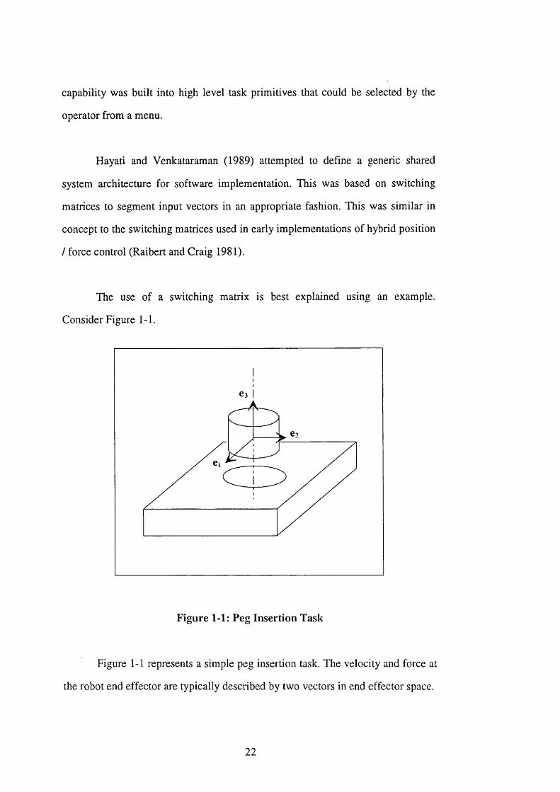
The use of a switching matrix is best explained using an example.
Consider Figure 1-1.
Figure 1-1: Peg Insertion Task
Figure 1-1 represents a simple peg insertion task. The velocity and force at
the robot end effector are typically described by two vectors in end effector space.
22
V ^ = [ V ; V j V j CO, CO; CO3 ] (1.1)
( 1.2)
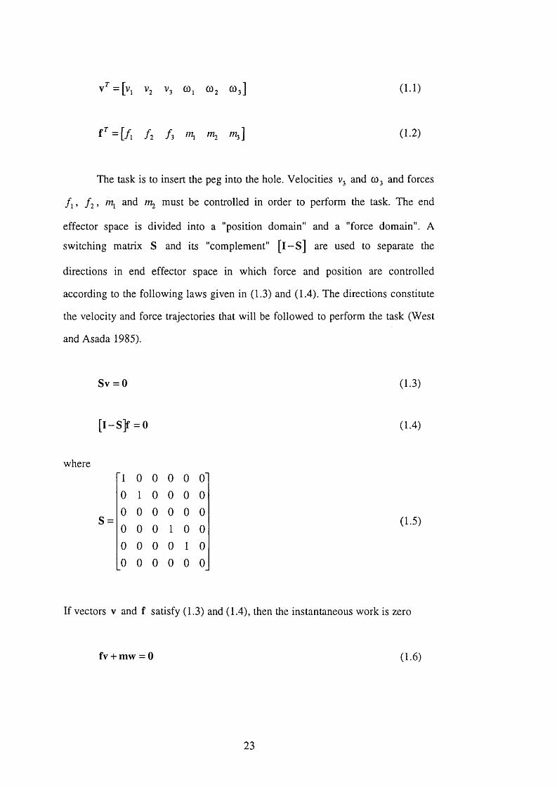
The task is to insert the peg into the hole. Velocities v. and CO3 and forces
f \ , and ni must be controlled in order to perform the task. The end
effector space is divided into a "position domain" and a "force domain". A
switching matrix S and its "complement" [ l - S ] are used to separate the
directions in end effector space in which force and position are controlled
according to the following laws given in (1.3) and (1.4). The directions constitute
the velocity and force trajectories that will be followed to perform the task (West
and Asada 1985).
S v = 0 (1.3)
(1.4)
where
S =
1 0 0 0 0 00 1 0 0 0 00 0 0 0 0 00 0 0 1 0 00 0 0 0 1 00 0 0 0 0 0
(1.5)
If vectors v and f satisfy (1.3) and (1.4), then the instantaneous work is zero
fv + mw = 0 ( 1.6)
23
Traditionally in shared control, the velocity command from the operator
and the force at the end effector is processed using a switching matrix to ensure
that ( 1.6) is satisfied.
It can be shown that the switching matrix does in fact embody a m etric or
measure. In order for the switching matrix to qualify as a proper physical law, it
must always produce correct results, even if the measurement reference frame is
moved. It can be shown that this quality is a function of how the metric is
transformed.
1.4 Main Contributions
In this dissertation, the focus is the theory of a parallel - non-combined
form of shared control, analogous to robotic hybrid position / force control.
The main contributions of this dissertation are put forward as follows:
• using an argument based strictly on modern differential geometry, the
switching matrix is shown to be equivalent to a filter which embodies a
Riemannian metric form. However, since the metric form is non-invariant, it is
shown that the metric form must undergo a transformation if the measurement
reference frame is moved. If the transformation is not made, then the switching
matrix fails to produce correct results in the new measurement frame,
• geometrically correct filters for shared control are given that are suitable for
inclusion into software and are demonstrated using a test harness,
24
• the switching matrix is shown to be a misinterpretation of a projection
operator,
• a correct theoretical description of shared control using a compliant
mechanism is presented,
• geometrically correct transformations for compliance control are given that are
suitable for inclusion into software and are demonstrated using a test harness,
• this work unifies recent results on robotic hybrid position / force control into a
consistent description based on modem differential geometry and Lie groups.
1.5 Comparison to Other Work
The closest works in concept to this dissertation are Lipkin (1985) and
Loncaric (1985).
Lipkin (1985) was the first to recognize that there was a flaw in the use of
a switching matrix for robotic hybrid position / force control. His argument was
based on the theory of screws (Ball 1900). Lipkin also derived correct filters for
robotic hybrid position / force control. This dissertation differs in the following
respects:
• the focus is on shared control rather than robotic hybrid position / force
control.
25
• the switching matrix is shown to be a misinterpretation of a projection
operator,
• an argument is formulated using the principles of modem differential
geometry.
Loncaric (1985) studied the implementation of compliance programming
for robotics from a modem perspective. This dissertation differs in the following
respects:
• the focus is on shared control rather than on compliance programming,
• the connection is made that the switching matrix is associated with a non
invariant Riemannian metric,
• the switching matrix is shown to be a misinteipretation of a projection
operator,
• the transformations required for invariant filtering are identified,
• algorithms for the implementation of geometrically correct schemes are
developed.
26
Chapter 2
Manifolds and Groups
2.1 Overview of the Chapter
Differential geometry provides an excellent, modem tool for discussing the
issues o f shared control. The theory generalizes our familiar ideas about curves and
surfaces to arbitrary dimensional objects called manifolds. However, the
mathematical concepts are abstract and require considerable interpretation before
they can be usefully employed to solve a practical engineering problem. Therefore,
rather than just referring the reader to the appropriate references, a clear and
concise interpretation o f the theory is presented here.
This Chapter is in six main sections. The first section details the basic
mathematical concepts behind modem differential geometry. The set o f all rigid
body displacements forms a group and this motivates a discussion on the theory o f
groups in the remaining sections.
2 7
2.2 Manifolds
Before a manifold can be defined, some basic definitions are required.
Definition 2.1 Topological Space
Let X be any set and T = g /} denote a certain collection o f subsets o f X .
The pair ( % ,r ) is a topological space if T satisfies the following requirements:
(i) 0 , ^ e r
(ii) if J is any (may be infinite) subcollection o f / , the family \U j \ j
satisfies kJ j^ U j g F .
(Hi) if K is any finite subcollection o f / , the family \U ^\k satisfies
X alone is often called a topological space. The are called the open sets and
F is said to give a topology to X (Nakahara 1990).
Definition 2.2 Neighbourhood
Suppose F gives a topology to X . is a neighbourhood o f a point x & X \ i N
is a subset o f X and N contains some (at least one) open set t/, to which X
belongs.
28
Definition 2.3 H ausdorff space
A topological space ( X ,r ) i s a H ausdo rff space if, for an arbitrary pair o f distinct
points X, x' G X , there always exist neighbourhoods o f x and U , o f x' such
that U ^r\U ^, = 0 . (Nakahara 1990).
Physical space is a topological space under a "sphere" topology. The
"sphere" topology is generated by the interior o f spheres o f arbitrary radius and
arbitrary centre. The topology consists o f all such open sets together with arbitrary
unions and finite intersections.
Physical space is a Hausdorff space since any two distinct points can be
encompassed by non-overlapping spheres o f sufficiently small radius.
An equivalence relation is now introduced under which geometrical objects
are classified according to whether it is possible to deform one object to the other
by continuous deformation.
Definition 2.4 Homeomorphisms
Let X, and X. . be topological spaces. A map f \ X ^ - ^ X ^ is a hom eom orphism
if it is continuous and has an inverse f ' ^ '.X^ X^ which is also continuous. I f
there exists a homeomorphism between X, and X . , is said to be
homeomorphic to X^ and vice versa (Nakahara 1990).
Definition 2.5 M anifold
M is an m-dimensional differentiable manifold if
(i) M is a Hausdorff space,
29
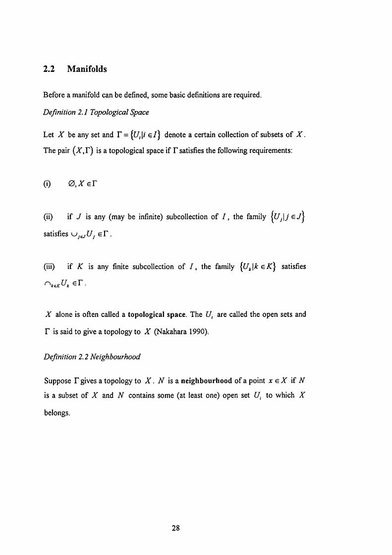
(ii) M is provided with a family of pairs ,
(iii) {[/, } is a family of open sets which covers M , that is w . [/. = M . <p is a
homeomorphism from (/,. onto an open subset U, ' of in'",
(iv) given and Uj such that t/, r \ U j ^ 0 y the map <py = from
Çj{Uir\Uj^ to ç>i(UfnUj^ is infinitely differentiable.
The pair is called a chart while the whole family {(f/jÇ?,)} is called an
atlas.
M
Figure 2-1: Differential manifold (adapted from Nakahara 1990)
30
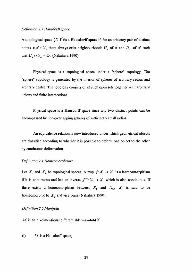
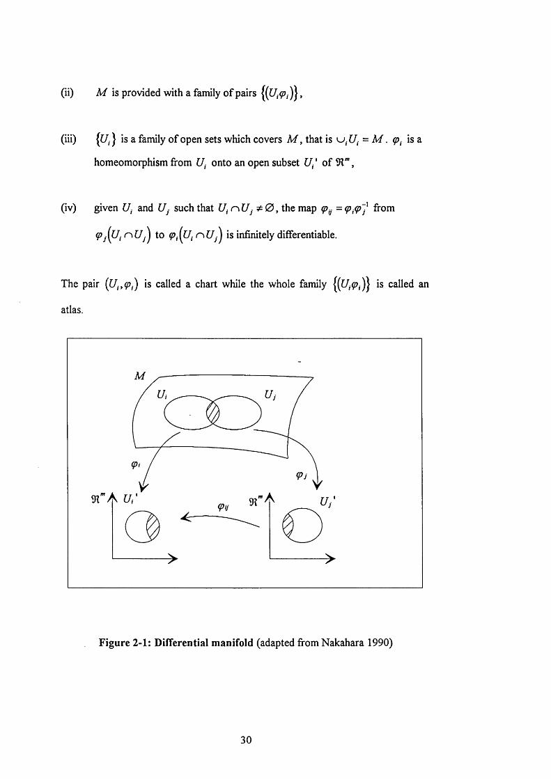
(p is the coordinate function. <p is represented by m functions
( / ? ) . . . . The set is called the coordinate.
The coordinate function corresponds to the assignment of a frame in U .
M
Figure 2-2: Coordinate function (adapted from Spivak 1979)
The dimension of the manifold M is the dimension of the space 9T".
(2 .1)
In three dimensional space, the surface of a unit sphere can be defined as
(2.2)
This is a two dimensional manifold, and the sphere is known as a two-
sphere. The two sphere has a higher dimensional analogue. For example, the three-
sphere is a three dimensional manifold in four dimensional space (Samuel et al
1991).
31
The formal mathematical generalization of "size" on a manifold is known as
a metric. If the metric is constant over the manifold, then the manifold is said to be
f la t .
Definition 2.6 Physical space
It is now possible to formally define physical space as a flat, orientable, 3
dimensional differential manifold, denoted by E .
E is assumed to be orientated, namely only a right handed orthonormal
basis will be considered.
The set (/?), is called the coordinate. The normal
(Euclidean) metric on E is the distance between points x and y .
i* > y |2 = ( (* -y )^ (* -y ) ) (% 3)
There is a family of Euclidean metrics on E , parameterized by the choice
of length scale.
Definition 2.7 Rigid body
A rigid body B a E is an open subset of E , the differentiable structure of
E naturally inducing one on B . B is said to be an open submanifold of E .
The formal definition of a submanifold is postponed until Chapter 3. The
boundary of a rigid body can be included but topological features such as edges
can mean the result is not a manifold.
32
2.3 Groups
Definition 2.8 SE{f)
Every rigid body displacement is an (internal) distance-preserving map,
known as an isometry. The set of all isometries of E forms a group, the special
Euclidean group, denoted SE{Z).
The special Euclidean group is the set of all maps
/:x i-> A x + d A e6 '0 (3 ),d er (3 ) (2.4)
S0{2) denotes a subgroup of the set of orthogonal groups, with
determinant +1, called rotations. 7(3) denotes the group of all translations.
Subgroups of the orthogonal group with determinant -1 (called reflections) are
not used.
Definition 2.9 Group
A group G is a set gy..g„ eG together with an operation, called group
multiplication (©) such that
(i) g , s G ,g , eG=> gi o g jS G (closure)
(>') g i°(g j°g i,) = (g i’‘S,)°gk (associativity)
(iii) g i ° g i= g i ° g i for all gj (existence of identity)
(iv) gk°gi = g i°g k = g I (unique inverse)
33

It is convenient to represent an element of SE(S) in matrix form:
g =A d 0 1
(2.5)
This representation is widely used in the robotics literature and is referred
to as a homogeneous transformation (Paul 1981). This representation is necessary
since displacements of 91" cannot be represented by wxw matrix transformations.
This inconvenience is removed by embedding 91" in 91" * as the n dimensional
hyperplane H . Linear transformations of 91" * exist that perform rigid
displacements in the hyperplane = 1 (McCarthy 1990).
To highlight the distinction, the set of (w + l)x (« + l) homogeneous
transforms is denoted H{n-\-\) rather than SEiri) .
Theorem 2-1
g ^H{A) fulfils the properties of a group.
Proof o f Theorem 2.1
Consider g, =
matrix multiplication, then
A, d," Aj d /and g =
0 1 0 1. If group multiplication is taken as
34
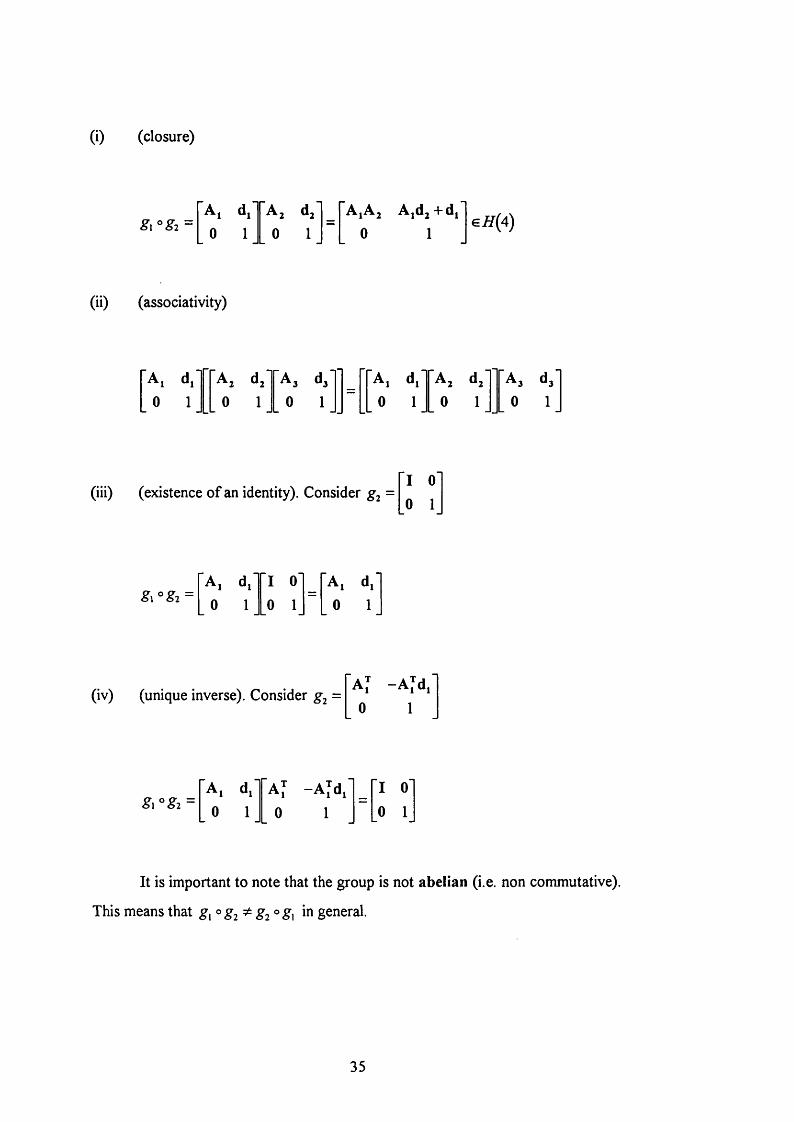
(i) (closure)
A, d. A: d. A,A% Ajd^+d,gx°gl = 0 1 0 1 0 1
;i/(4 )
(ii) (associativity)
A, d, 0 1
A j d j
0 1d)
0 1
A, d ,j A j dj 0 1 0 1
A j d j
0 1
(iii) (existence of an identity). Consider =I 00 1
A, d .T l o' A, d,'0 l i o 1 0 1
(iv) (unique inverse). Consider = A l - A id ,
0 1
g^°g2 =A, d|' "a I -A id , I o'0 1 0 1 0 1
It is important to note that the group is not abelian (i.e. non commutative).
This means that g^^gi^ gi °g\ in general.
35
One further definition will be required:
Definition 2.10 Diffeomorphism
A difTeomorphism is a infinitely ( C" ) differentiable homeomorphism.
Diffeomorphisms classify spaces into equivalence classes according to
whether it is possible to deform one space to another smoothly (Nakahara 1990).
The set of diffeomorphisms is a group denoted by Diff (M ) .
2.4 Lie Groups
A Lie group is a manifold on which group multiplications, product and
inverse, are defined.
Definition 2.11 Lie group
A Lie group G is a differentiable manifold which is endowed with a group
structure such that all group operations
(i) • : G x G ^ G by
(ii) ■':G -> G by
are differentiable (Nakahara 1990).
SEif) has the structure of a Lie group.
36
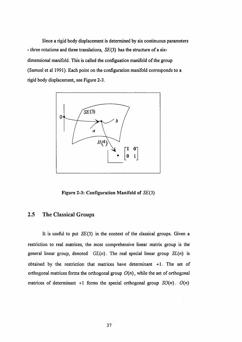
Since a rigid body displacement is determined by six continuous parameters
- three rotations and three translations, SE(3) has the structure of a six
dimensional manifold. This is called the configuation manifold of the group
(Samuel et al 1991). Each point on the configuration manifold corresponds to a
rigid body displacement, see Figure 2-3.
Figure 2-3: Configuration Manifold of SE(3)
2.5 The Classical Groups
It is useful to put SE(3) in the context of the classical groups. Given a
restriction to real matrices, the most comprehensive linear matrix group is the
general linear group, denoted GL{n). The real special linear group SL{n) is
obtained by the restriction that matrices have determinant +1. The set of
orthogonal matrices forms the orthogonal group 0{n) , while the set of orthogonal
matrices of determinant +1 forms the special orthogonal group SOin) . 0{n)
31
consists of two disconnected pieces, with SO{ri) occurring as a subgroup
(Wyboume 1974).
SO{n) leaves invariant the symmetric bilinear form
(x ,y ) = Z ^ V (2.6)i= l
GL{n) is a Lie group where the product of elements is simply the matrix
multiplication and the inverse is given by the matrix inverse. SL{n) and SO{ri) are
Lie subgroups of GL{n) .
Next consider the skew symmetric bilinear form in a (necessarily even) In
dimensional vector space
(x ,y )= (% y + ' - % - Y ) 4 - ( % y + ' _
= x^Jy
with J = 0T 0
(Sattinger and Weaver 1986).
Matrices which leave this form invariant satisfy A JA = J and constitute
the non-compact symplectic group Sp(2n) .
Before SE{3) can be classified, some further definitions are required.
38
Definition 2.12 Product group
If Gi and Gj are two groups, the product group G = G, x G is the set of pairs
(^1,^2) , g, in G, and in with the group law
g i ) = i .g igx' ,g ig i) (2-8)
Definition 2.13 Semi-direct product
if Vg, gG, , V^2 gGj , g j—^^^'gz, the semi-direct product of G by G, is the
set of pairs (gpgj) with the following group law (Normand 1980)
igx,gj.gx g i ) = (29)
where
g i ‘' g i = g \ g t + g i (2 1 0 )
It is now possible to classify 5E(3) as a semi-direct product of the abelian
invariant subgroup of translations T(3) by the classical subgroup SOif) .
2.6 The Rotation Group SOif)
It is easy to see why A egG(3) must be an orthogonal matrix. Consider
the Euclidean metric if a rigid body undergoes a displacement:
IKy|l2=l|(Ax + d),(Ay + d)|| = ( (x -y )’'A’'A (x-y))
39
For the metric to be invariant (i.e. for internal points to preserve their
distances), then A A = I Therefore A e^ (9 (3 ) must be orthogonal (McCarthy
1990).
Every rotation A e S0(3) can be parameterized by an axis of rotation n
and the angle 0 of rotation about this axis: A = ( n ,0 ) . It should be emphasized
that this parameterization is intrinsic i.e. independent of any choice of basis. The
axis requires two angles for its specification, so three parameters are needed to
specify a general rotation; S0(3) is a three parameter group (Sattinger and Weaver
1986).
The range of angle used in any parameterization is an important issue
(Altmann 1986). It is shown later that it is important that the neighbourhood of the
identity of iS(9(3) (the zero angle) be contained in the range. For this reason, the
range is normally represented, for some angle 0 : - 7t <0 < tc . There are a number
of choices for the parameterization. Here a rotation is taken in terms of rotations
about a right handed orthonormal basis {e,, e , , 63}.
A (ep0 ) =
1 0 0
0 COS0 - s in 0
0 sin0 COS0
(2 . 12)
A(C2,0) =
COS0 0 sin0
0 1 0- s in 0 0 COS0
(2.13)
40
A (e ,,^ ) =
cosO -s in^ 0 sin^ cos 9 0
0 0 1(2.14)
This representation is weak in the sense that rotations do not commute but
it has certain properties in the neighbourhood of the identity which makes it useful
(Altmann 1986).
2.6.1 The Configuration Manifold Structure of S0[3)
To define the configuration manifold structure of S0(3), symbol is
introduced to represent a single vector parameter - a vector parallel to the rotation
axis with modulus equal to the rotation angle (Altmann 1986). Then A(^n) is
called the parametric point. By continuously varying the direction of n and angle
9, the parametric point traces a three ball of radius tt . This defines the
configuration manifold structure and is sometimes referred to as the parametric ball
of S0{3) (Samuel et al 1991).
Diametrically opposite points on the surface of the parametric ball are
not distinguished from each other. One can imagine that each antipodal point is
linked in some manner to its podal point in such a way that when a parametric
point reaches the surface of the ball, it jumps back from it to the corresponding
podal point.
The identity of S0(3) is parameterized by the vector (On) i.e. the centre of
the parametric ball. The motivation behind the choice of range is now clear - the
41

identity and its neighbourhood are well away from the surface of and its
eccentric topology (Altmann 1986).
In the next chapter, the infinitesimal properties of Lie groups are studied,
that is, the properties of the group near the identity element. This leads in a natural
way to the important concepts of the infinitesimal generator and Lie algebra. These
concepts allow a formal description of the velocity of a rigid body.
42
Chapter 3
Calculus on Manifolds
3.1 Overview of the Chapter
In this Chapter, the calculus on manifolds is developed. This leads to the
important concept of a tangent space on a manifold. The theory is linked at each
stage to SE(3) and the infinitesimal operators for the subgroups are derived. The
Lie algebra for the Lie group SE(3) is examined and is shown to be a semi-direct
sum of the Lie algebra associated with T(3) and S0(3) .
3.2 Tangent Vector
Before a tangent vector can be defined, some preliminary definitions are
required.
Définition 3.1 Open curve
An open curve in an w-dimensional manifold A/ is a map c:{a,b)-> M where
(a,A) is an open interval such that a < 0 < b (Nakahara 1990).
43
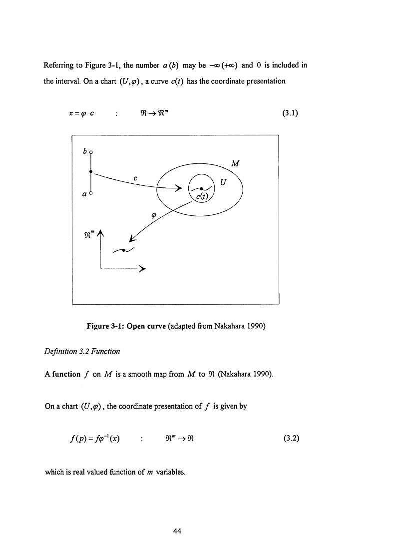
Referring to Figure 3-1, the number a{b) may be -oo (4-00) and 0 is included in
the interval. On a chart (JJyÇ) , a curve c{i) has the coordinate presentation
x = (p c (3.1)
c{t)
Figure 3-1: Open curve (adapted from Nakahara 1990)
Definition 3.2 Function
A function / on M is a smooth map from M to 91 (Nakahara 1990).
On a chart (C/, (p) , the coordinate presentation of / is given by
(3.2)
which is real valued function of m variables.
44
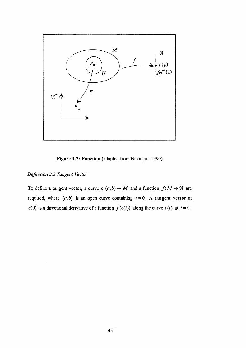
Figure 3-2: Function (adapted from Nakahara 1990)
Définition 3.3 Tangent Vector
To define a tangent vector, a curve c: {afi) —> M and a function / : % are
required, where (ar,6) is an open curve containing / = 0. A tangent vector at
c(0) is a directional derivative of a function / (c(/)) along the curve c{t) at / = 0.
45
X (c{t))
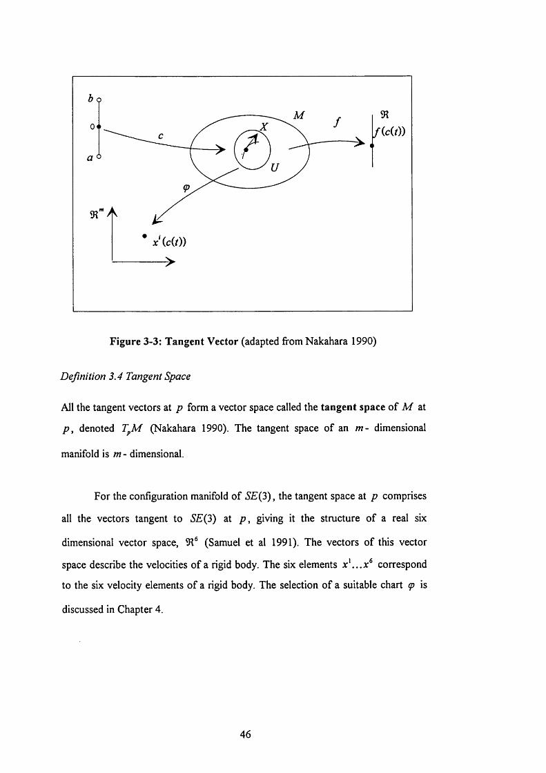
Figure 3-3: Tangent Vector (adapted from Nakahara 1990)
Définition 3.4 Tangent Space
All the tangent vectors at p form a vector space called the tangent space of M at
/?, denoted T^M (Nakahara 1990). The tangent space of an m- dimensional
manifold is w - dimensional.
For the configuration manifold of SE(3), the tangent space at p comprises
all the vectors tangent to SE{3) at p , giving it the structure of a real six
dimensional vector space, 91 (Samuel et al 1991). The vectors of this vector
space describe the velocities of a rigid body. The six elements x\..x^ correspond
to the six velocity elements of a rigid body. The selection of a suitable chart q> is
discussed in Chapter 4.
46
3.3 Infinitesimal Operator
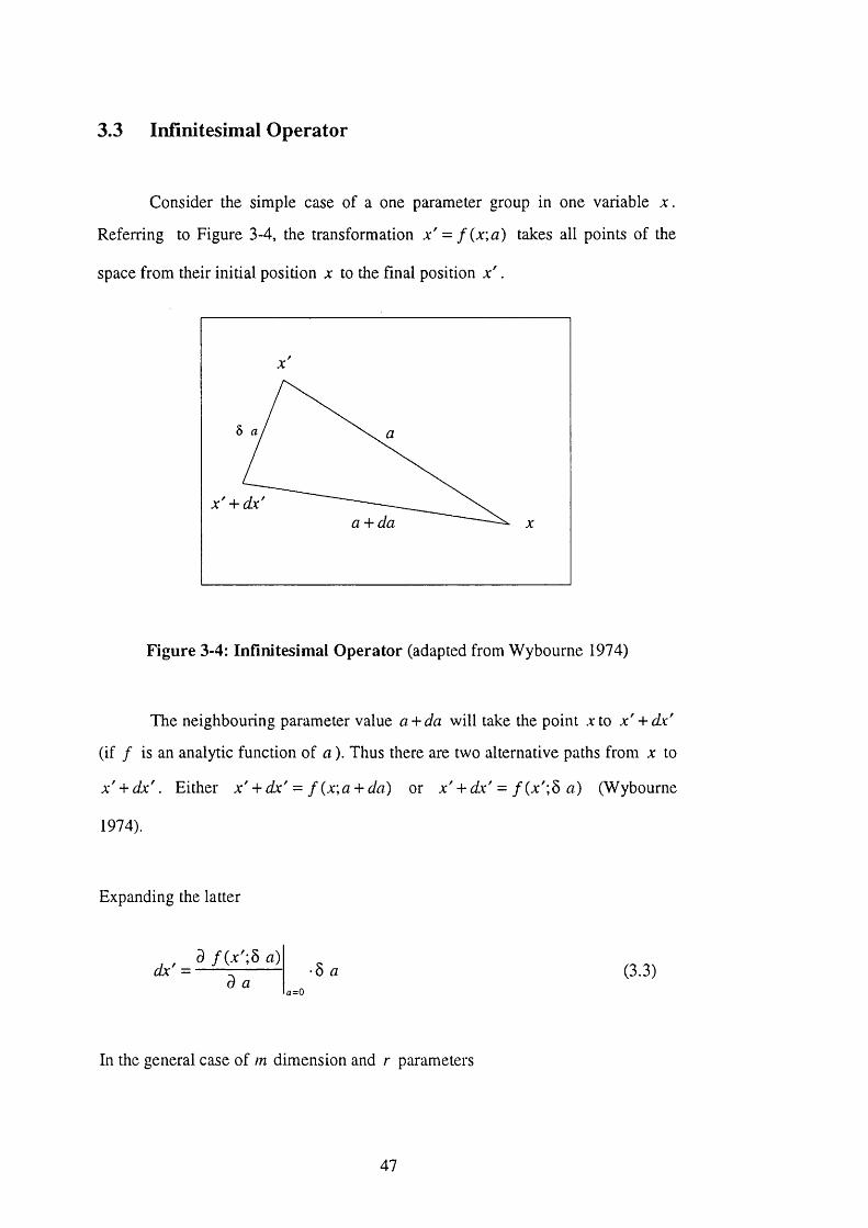
Consider the simple case of a one parameter group in one variable
Referring to Figure 3-4, the transformation .v '= f ( x ; a ) takes all points of the
space from their initial position x to the final position x ' .
x ' -\-dx'a + da
Figure 3-4: Infînitesimal Operator (adapted from W ybourne 1974)
The neighbouring parameter value a + da will take the point x to x ' + dx'
(if / is an analytic function of a ). Thus there are two alternative paths from x to
x + d x ' . Either x ' + d x ' - f {x\a +da) or x ' + d x ' = f { x ' a ) (Wybourne
1974).
Expanding the latter
0 / ( . r ' ; 5 a)dx' =
d a•Ô a
a=0
(3.3)
In the general case of m dimension and r parameters
47
{dx) = Xd /* (x ';5 a)
•h i = a = l...r (3.4)a=0
or <ix'= U ' ( x ) -5 rz' (3.5)
The infinitesimal transformation x ' ^ x ' + d\ ' induces
f i x ' ) / ( x ' ) + <ÿ(x ') (3.6)
# ( > ■ ) -
6 y ( x ' ) = 8 a ^ X ^ ( / ) (3.7)
where X„ = U '
It is now possible to define the infinitesimal operator of the group as
ui' " a /
(3.8)
48
3.4 Infinitesimal Operator of T(3)
In the case of 7 (3 ), and expressing matrices in the hyperplane
Xi 1 0 0 1X2 0 1 0 «2 X2
X3 0 0 1 a, 31 0 0 0 1 __ 1
(3.9)
/ / ■+ Jxi "1 0 0 5 fli
/
X2 -\-dX2 0 1 0 Ô Ü2 X3
• 3 + dx^ 0 0 1 5 3 X3
1 0 0 0 1 1
(3.10)
Therefore,
jCj +dx^ - X; + 5 <3j (3.11)
+ dx^ = Xt + Ô (3.12)
A*3 + dx^ = X3 + 5 «3 (3.13)
Taking derivatives
(x. +6 a,) = i (3.14)
49
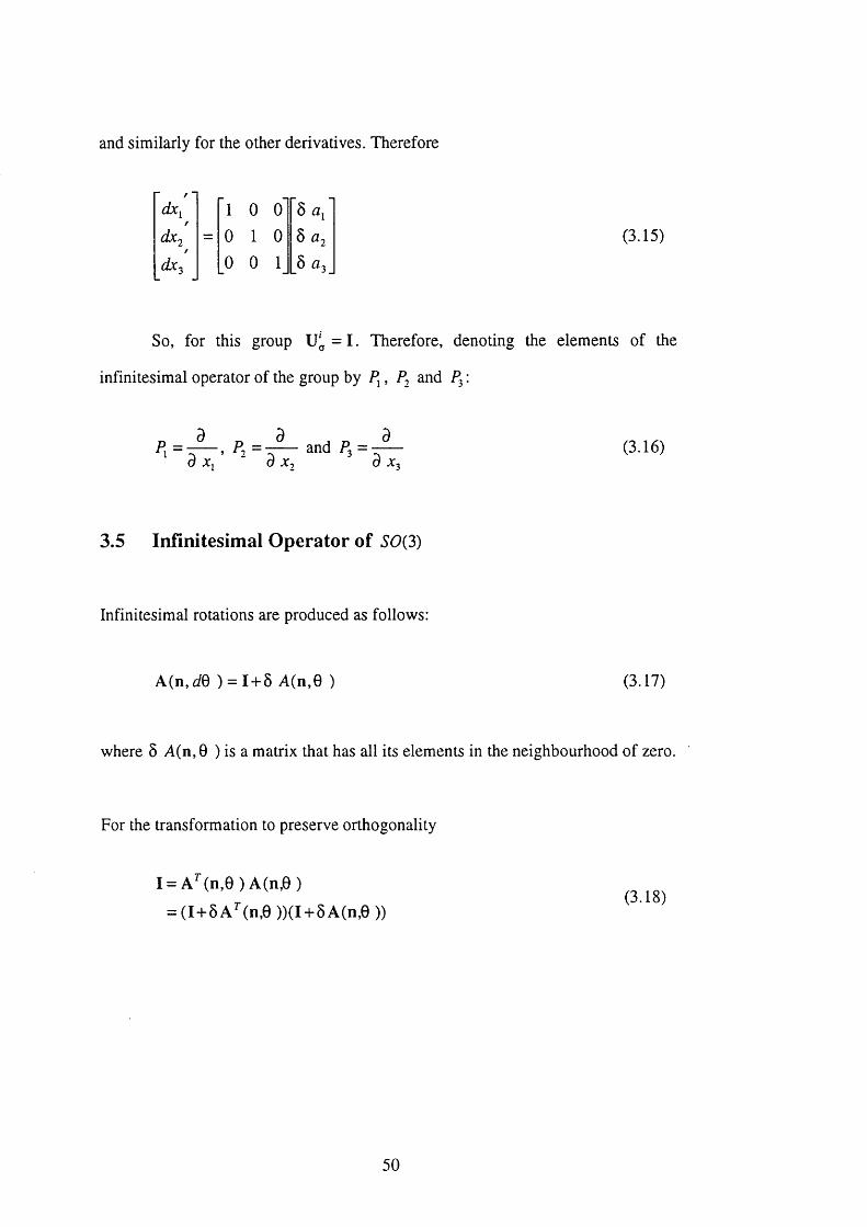
and similarly for the other derivatives. Therefore
/ -dx^ ’1 0 o' 6dxj = 0 1 0 5 Ü2
dx^ 0 0 1 5 a,_(3 15)
So, for this group = I Therefore, denoting the elements of the
infinitesimal operator of the group by , P, ^rid P3 :
Pj = T— , Pj = and P3 =d “ d X2
(3.16)
3.5 Infinitesimal Operator of 5(9(3)
Infinitesimal rotations are produced as follows:
A(n,dQ ) = I + 5 A(n,0 ) (3T7)
where 5 A(n,0 ) is a matrix that has all its elements in the neighbourhood of zero.
For the transformation to preserve orthogonality
I = A’'(n,e)A(n,6)
= (I+5A''(n,e))(I+8A(n,e))(3.18)
50
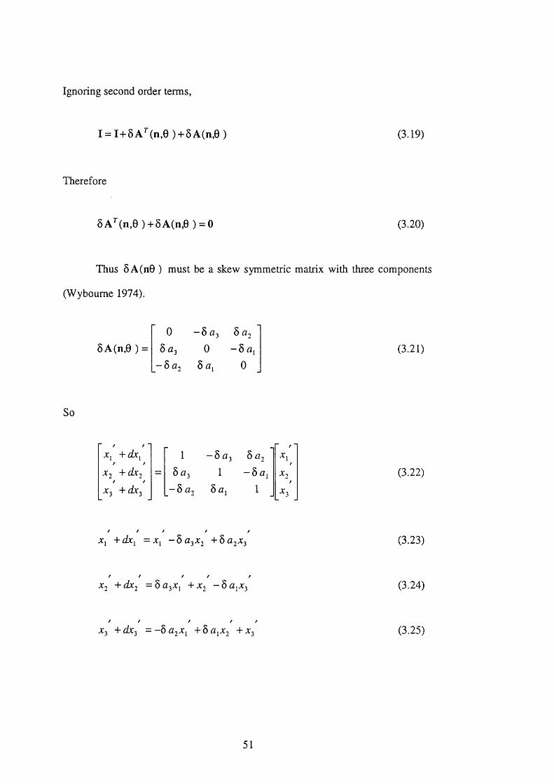
Ignoring second order terms,
I = I+8A^(n,e) + 5A(n,e) (3,19)
Therefore
8A^(n,8)+8A(n,8) = 0 (3.20)
Thus 5 A( n8 ) must be a skew symmetric matrix with three components
(W yboume 1974).
0 - 8 ^ 3 8 ^ 2
5A (n,8 ) = 8 # 3 0 — 8 f l j CL21)
— 8 # 2 8 0
So
/ / *A] 1 -8&3 8 #2
- , -
. 2 +< 2 = 8^3 1 — 8 A2 (3.22)
A3 +dx. - 8&2 8 «I 1 / 3
-\-dx^ +Ô <3,- 3 (3 23)
-\-dx^ = da^x , + x , - b a , x1- 3 (3.24)
a'3 + Zx'3 = -Ô +6a^X2 +X 3 (3.25)
51
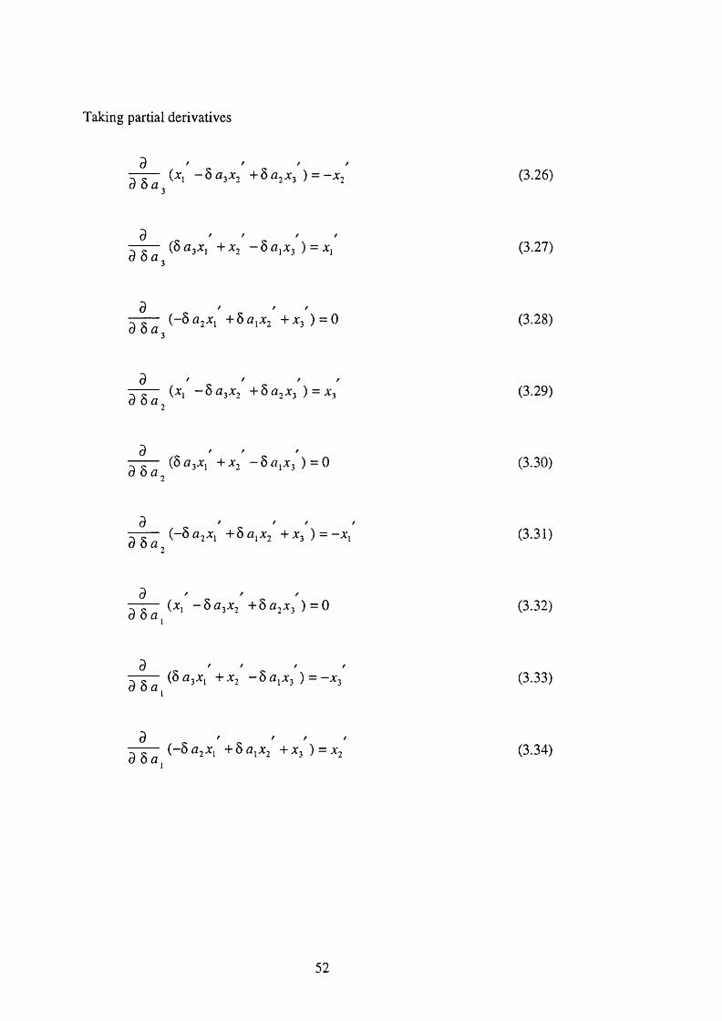
Taking partial derivatives
d- 5 « 3 ^ 2 + 8 ^ 3 X3 ) = - % 2 (3.26)
8 » ' ' - ' '(8 3%, +Xj -8a;%3 ) = (3.27)
8 8 a ,
8 /(-8 a^x +8a .%2 +-^3) = 0 (3.28)8 8 a ,
8 ' '(%i - oa^Xj + 8 a 2 % 3 ) = % 3 (3.29)
8 8 a
(8 0 3 . ^ 1 + X 2 - 8 a ^ % 3 ) = 0 (3.30)8 8 a \
88 8 a ,
88 8a^
(-8a7%^ 4-8ai%2 4-%3 ) = (3.31)
(%i - ba^Xj 4-8a.X; ) = 0 (3.32)
( 8 a 3 X; 4-%2 - 8 ai ^ 3 ) = -.x: 3 (3.33)8 8 a^
/ / f8 /(-8 a 2 %i 4-8a^%2 4- %3 ) = % 2 (3.34)8 8 a ,
52
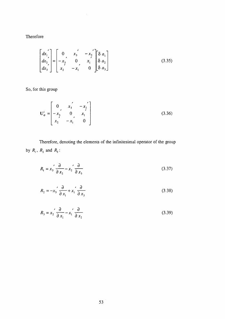
Therefore
f -
d x ^
f f -
0 % 3 - j r . 5
d x j - - % 3 0 x ^ 8 Û 2 (3.35)d x ^ x ^ - x ^ 0 _ 5 a , _
So, for this group
0 JC3 - X j
u ; = - X j 0 • 1 (3.36)Xi “ ■1 0
Therefore, denoting the elements of the infinitesimal operator of the group
by /?i, /?2 and :
' 3 ' 3(3 37)
' 3 ' 3R. = -X-, - — + X
3 JC] 3 JC3
(338)
' 3 ' 3
*3 = a T " ^ ‘ a T(3.39)
53
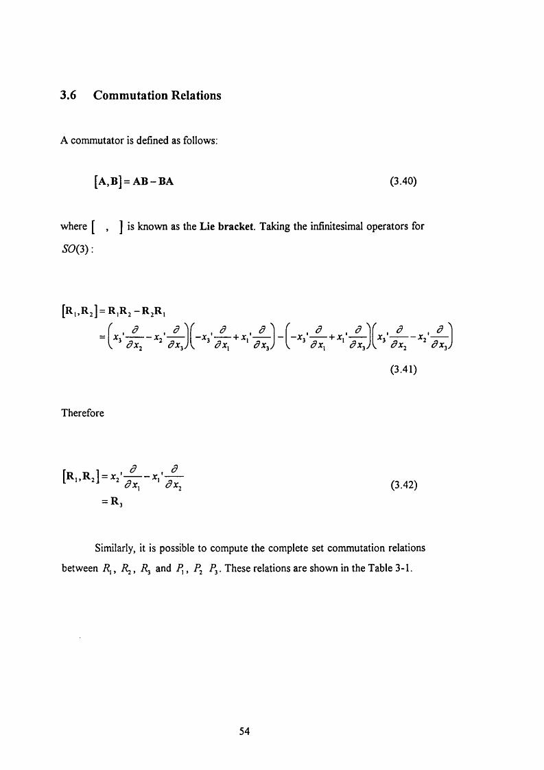
3.6 Commutation Relations
A commutator is defined as follows:
[A,B] = A B -B A (3.40)
where [ , ] i s known as the Lie bracket. Taking the infinitesimal operators for
^ 0 (3 ) :
[R,.R;] = R ,R ;-R ,R ,
3/ V dXy d x j- x ' ^ + x,- ^ - x ^
âx^ âx^J\ âx^ âx^J
(3.41)
Therefore
[R„R,] = x , ' - / — X/-ÔX^ ôx^ (3 42)
= R
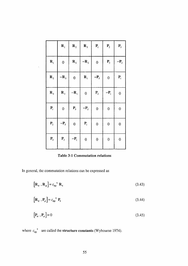
Similarly, it is possible to compute the complete set commutation relations
between and P , P2 P . These relations are shown in the Table 3-1.
54
R. Ri R, P, Pi P3
R. 0 R3 -R i 0 P3 -Pi
«2 -R3 0 R. -P3 0 P.
R, R, -R , 0 Pi -P. 0
P. 0 P3 -Pi 0 0 0
Pi -P3 0 P. 0 0 0
P3 Pi -P, 0 0 0 0
Table 3-1 Commutation relations
In general, the commutation relations can be expressed as
[ R , , R p ] = c , ; R ,
[ CT »Pp]=^(Tp Pc
[Pa .Pp] = 0
(3.43)
(3.44)
(3.45)
where are called the s tru c tu re constan ts (Wybourne 1974).
55
The structure constants for each infinitesimal operator can be assembled
into a matrix, . If the elements of are set as follows
(3-46)
then the matrix is identical to the basis for the tangent vector.
3.7 Lie Algebra
Definition 3.5 Lie algebra
Let A be an r - dimensional vector space over field K in which the law of
composition for vectors is such that to each pair of vectors X and Y there
corresponds a vector Z = [X, V] in such a way that
(i) [aX +/?Y ,Z ] = a[X,Z]+>3[Y.Z]
(ii) [X,Y]+[Y,X] = 0
(iii) [X, [Y, Z]] + [y . [Z, X]] + [Z, [X, Y]] = 0 (Jacobi Identity)
for all gK and all X ,Y ,Z g A.
A vector space A satisfying the above commutator relationships constitutes a Lie
algebra (Wyboume 1974).
56
A given Lie algebra is said to be real if K is the field of real numbers and
complex if K is the field of complex numbers. The Lie algebra associated with a
Lie group is always real. For every Lie group there is a Lie algebra and for every
Lie subgroup there is a subalgebra. The Lie algebra associated with a Lie group is
denoted by the same letter as for the group, but in lowercase (Wyboume 1974).
The Lie algebra of SE{3), denoted 5e(3), is generated by the three
infinitesimal rotation operators given in (3.37) to (3.39) and the three infinitesimal
translation operators given in (3.16). For example, take X j= R j , Y = and
[a R, +>3 R„P,] =[a R„P3]+[/? R „P,]
= a [ R , . P , ] + f [R;.P,]
[R ,.[R 2.P3]]+ [R 2.[I’3 .R ,]]+ [P3.[R ,.R2]]
= [R„P,] + [R3,P3] + [P„R3] = 0
3.7.1 Lie subalgebras
A subset H of a Lie algebra A is called a subalgebra of A if S is a linear
subspace of A and
[X, Y] e E for any (X, V e E) (3.47)
57
A subalgebra S of A is said to abelian if
[X, Y] = 0 for any (X, Y e E) (3.48)
The algebra f(3) associated with the subgroup T(3) is an abelian
subalgebra of ^ (3) (Wyboume 1974).
3.7.2 Ideals
A subset H of A is said to form an ideal or invariant subalgebra of A if H is a
linear subspace of A and
[X ,Y ]eS forany (X ,6 E ,Y 6 A ) (3.49)
If the algebra contains members that are not in the ideal, then the ideal is
said to a proper ideal. In this case it is important to note that the identity element
is always a member of the algebra. By restricting attention to proper ideals, the
improper ideals formed by the whole algebra and by the subset containing the
identity element are eliminated (Wyboume 1974).
Therefore, f(3) forms a proper ideal of jg(3).
3.7.3 Simple and Semisimple Lie algebras
A Lie algebra is said to be simple if it contains no proper ideals. The algebra is said
to be semisimple if it contains no abelian ideals except the subset containing the
identity element (Wyboume 1974).
58
Although it is possible to assess se(3) by inspection, it is useful to
introduce a simple test for deciding if a Lie algebra is semisimple. The test is based
on the Killing metric defined in terms of structure constants (Gilmore 1974).
Theorem 3.1 Carton's test for a semisimple Lie algebra
A Lie algebra is semisimple if and only if
d e t|^ < rth ° (3.50)
where is the symmetric Killing metric defined in terms of structure constants:
SaX - ^ap ^Xz^
Proof of Theorem 3.1
see Wyboume (1974).
For jg(3), for example
^12 ^13 "^^13 ^12 "^^15 ^16 *^^16 ^15
= (1)(_1)+(_1)(1) + (1)(_1)+(_1)(1) (3.51)
= -4
Similarly g = -4 and g = -4 . The remaining elements are zero. Therefore
- 4I 3 O3 O3 O3
(3.52)
Now det|g| = 0, so the Lie algebra 5e(3) is not semisimple.
59
However the Killing metric for SOQ) is given by
« = [ - 213] (3.53)
Now det|g| = - 8 , so the Lie algebra so(3) is semisimple.
3.7.4 Solveable Lie algebras
The derived algebra of a Lie algebra A is formed by taking the set of all
linear combinations of elements that can be expressed as commutations of the
elements of A
A "> = [A ,A ] (3.54)
It is possible to form a whole series of derived algebras. If the k th derived algebra
A = [a , A *■* ] , then the series
A,A('\..A(") (3.55)
is called the derived series of the Lie algebra A (W yboume 1974).
If for some positive integer k ,
A(") = 0 (3.56)
the Lie algebra A is said to be a solveable Lie algebra. S E (3) does not have a
solveable Lie algebra but 7(3) does since = [P , P ] = 0 .
60
3.7.5 Direct and Semidirect Sums
A Lie algebra A is a direct sum of Lie subalgebras
A = A ,©A 2©...©A„ (3.57)
if for every pair of subalgebras A, , Ay
A,.nAy = 0 (3.58)
Any Lie algebra A can be written as a semidirect sum
A = A,©,A2 (3.59)
of a solveable Lie algebra A, and a semi-simple Lie algebra A^.
3.7.6 Classification of se(S)
The Lie algebra se(3) cannot be expressed as a direct sum but can be
expressed as a semidirect sum of the solveable Lie algebra f(3) and the semi
simple Lie algebra so(3) :
se(3) = /(3)e^so(3) (3.60)
61
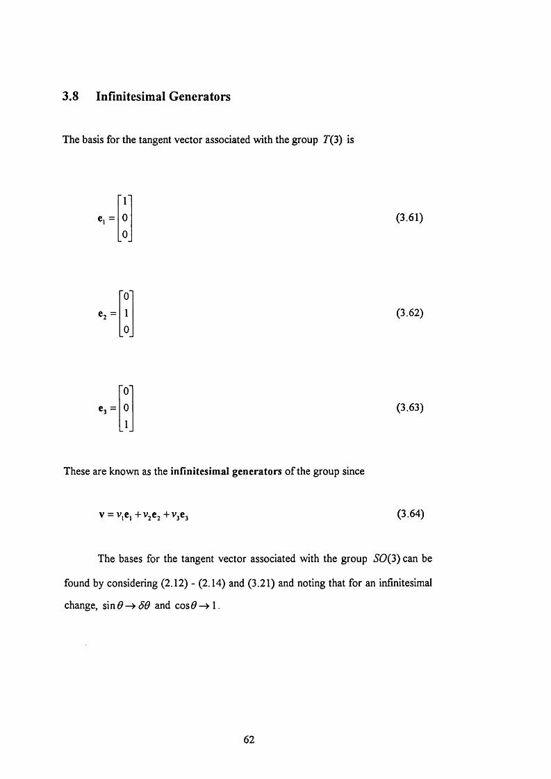
3.8 Infînitesimal Generators
The basis for the tangent vector associated with the group T(3) is
Cl = (3.61)
(3.62)
e, = (3.63)
These are known as the infinitesimal generators of the group since
v = v,e,+V2e2+V3e3 (3.64)
The bases for the tangent vector associated with the group S0(3) can be
found by considering (2.12) - (2.14) and (3.21) and noting that for an infinitesimal
change, sin^->^^ and co s^ -> l.
62
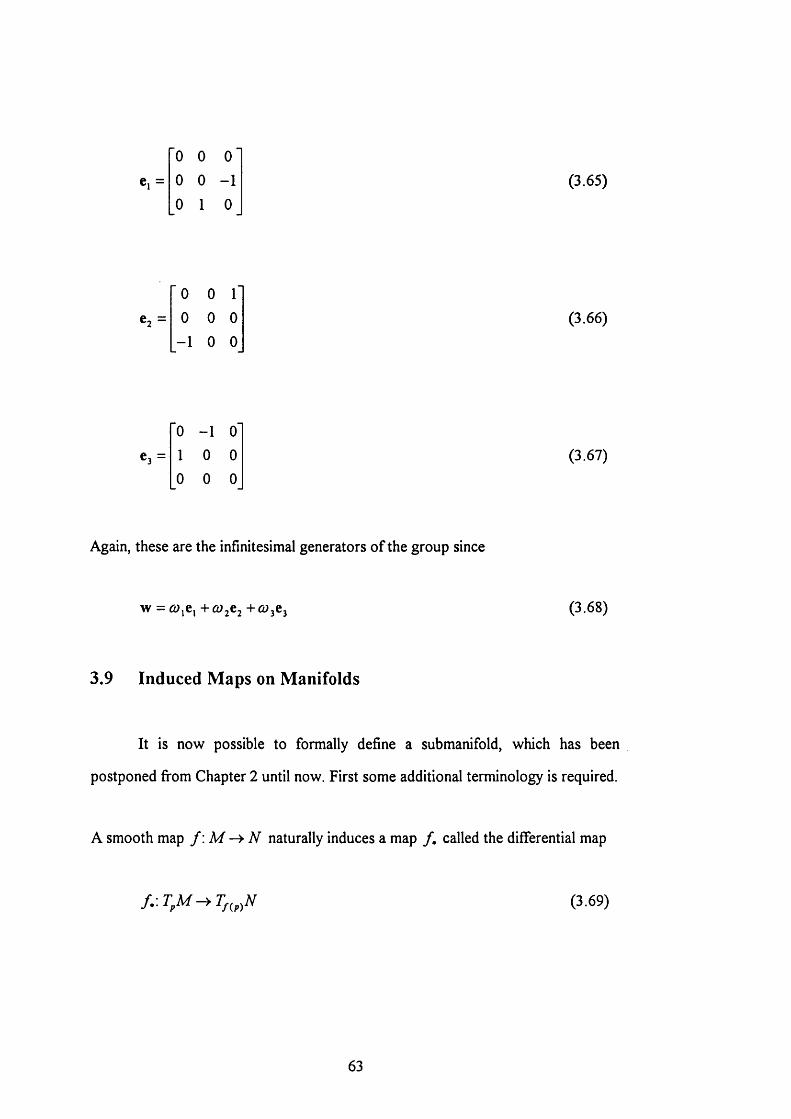
e, =
0 0 00 0 - 1 0 1 0
(3.65)
G] =
0 0 10 0 0
- 1 0 0(3.66)
e, =0 - 1 0 1 0 00 0 0
(3.67)
Again, these are the infinitesimal generators of the group since
(3.68)
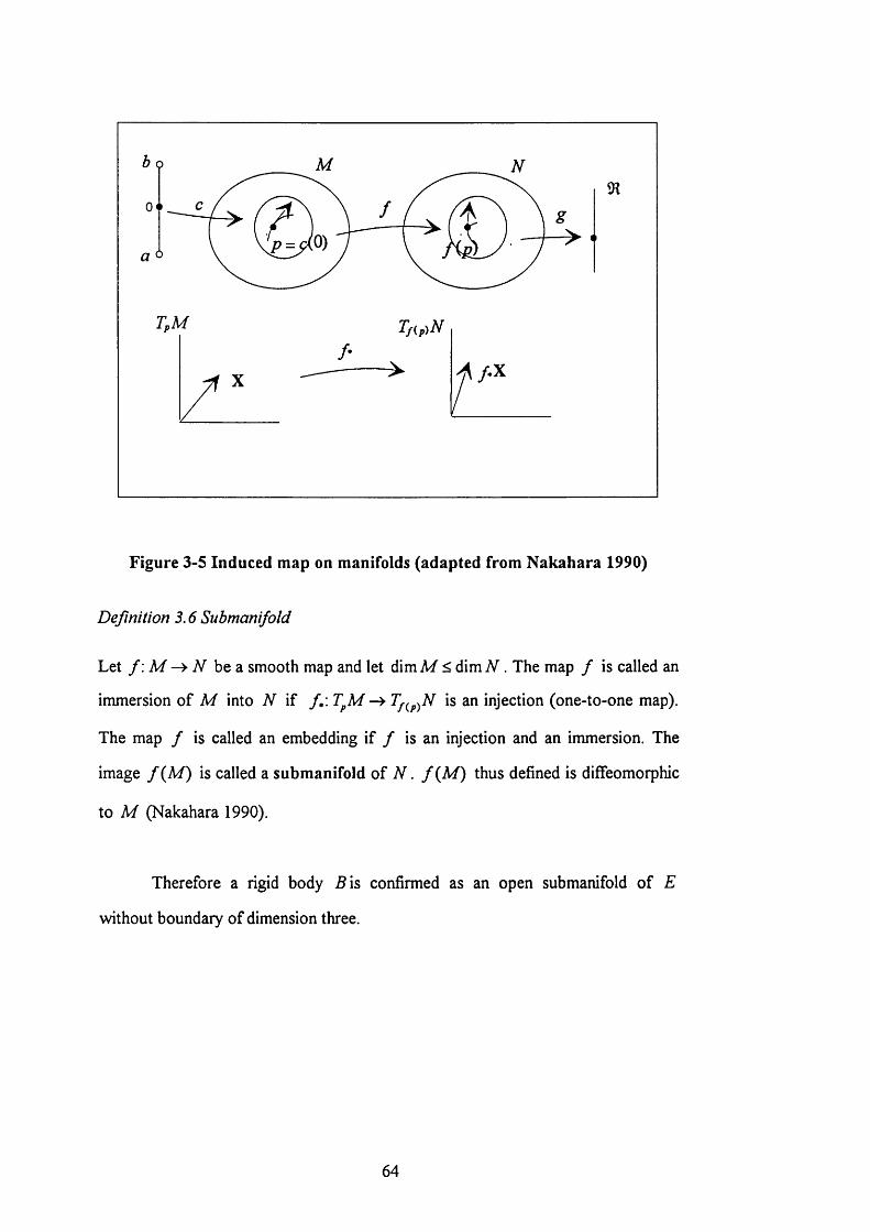
3.9 Induced Maps on Manifolds
It is now possible to formally define a submanifold, which has been
postponed from Chapter 2 until now. First some additional terminology is required.
A smooth map f : M - ^ N naturally induces a map / . called the differential map
(3.69)
63
M
A f.X
Figure 3-5 Induced map on manifolds (adapted from Nakahara 1990)
Definition 3.6 Submanifold
Let f : M - ^ N be a smooth map and let dimM < dim N . The map / is called an
immersion of M into N if /*: is an injection (one-to-one map).
The map / is called an embedding if / is an injection and an immersion. The
image / (M) is called a submanifold of N . f (M) thus defined is diffeomorphic
to M (Nakahara 1990).
Therefore a rigid body B\s confirmed as an open submanifold of E
without boundary of dimension three.
64
Chapter 4
Representation of the Lie algebra of the Special Euclidean Group
4.1 Overview of the Chapter
In this chapter the matrix representation of se(3) is introduced.
Representations in an inertial and body fixed frame are developed. The effect of a
displacement of the reference frame leads to the important concept of the
differential map. This has relevance in both fixed frame representations and moving
frame representations. Lastly, an original review of the application of the theory of
Lie groups in robotics is given, with particular reference to the exponential map.
4.2 Matrix representation of jg(3)
For the group SE(3) , and using the map given in (2.4)
x'=Ax + d (4.1)
Differentiating both sides of (4.1) with respect to time
65
Differentiating both sides of (4.1) with respect to time
x ' = Ax + d
= À A ^ ( x '- d ) + d04.2)
where ÀA^ is the angular velocity of the rigid body relative to an inertial
frame, and - ÀA d + d is the translational velocity of a point on the rigid body as
it passes through the origin of the inertial frame. This is referred to as the inertia l
rep resen ta tion (Park and Brockett 1994).
In hyperplane matrix form
■x'‘ À d ' A^ -A ^ d ^ fx '-
_ 1_ 0 0 0 1 [ 1_
‘ÀA^ -À A ^ d + d ' x'"
0 0 1
04.3)
Denoting
À d ' A^ -A ^ d 'X = and X"‘ =
0 0 0 1
the inertial velocity representation can be written as XX~^. An alternative
representation is the body fixed rep resen ta tion written as X X (Park and
Brockett 1994).
66
In this case
x ' A^ - A ^ d À d" x '
1 0 1 0 0 1
' a ^à A ^ d ' x '
0 0 _ 1
(4 .4 )
A^À is the angular velocity of the rigid body relative to the instantaneous
body frame and A ^d is the translational velocity of the rigid body relative to the
instantaneous body frame. This representation is also known as a left invariant
vector field on SE{3) and is the more natural choice for analysis of the shared
control of rigid bodies.
Taking the group 5 0 (3 ) , the orthogonality condition is A A = I
Differentiating both sides
A 'A + A ^ A = 0 (4.5)
Therefore A^À is a skew symmetric matrix, denoted Q.. This means that the
combination [Q A^d] which consists of a skew symmetric matrix and a vector,
determines by its values at a certain instant, the velocity of all points at that
instant. The bases for Q are given in (3.65) - (3.67) and the bases for A ^d are
given in (3.61) - (3.63). Therefore
a v'
0 064.6)
67
0 -CO, CO,where f l = CO, 0 -Û3, (4.7)
-CO2 CO, 0
V = A d = (4 8)
The skew symmetric form is so useful that a special notation is used as follows
[xj = 3 0 -X,X
-^2 1
0*9)
Therefore
g = x - ‘x =[w j V
0 0gsse(3 ) (4.10)
It can be convenient to construct g as a column vector of dimension six.
g =wV
This representation is sometimes referred to as a screw. This representation
should be treated with some caution. To explain this, it is appropriate to be more
68
specific about our definition of . In this thesis, 91* is used solely to denote the
real six dimensional vector space and not a six dimensional Euclidean metric space.
Since all real vector spaces of the same dimension are isomorphic, Jg(3) is
isomorphic to 91* (Selig 1995). However, je(3) is not a six dimensional Euclidean
metric space. This distinction is often missed and can lead to erroneous use of
metrics on the vector space.
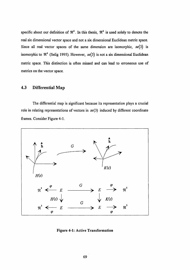
4.3 Differential Map
The differential map is significant because its representation plays a crucial
role in relating representations of vectors in se(3) induced by different coordinate
frames. Consider Figure 4-1.
Kit)
Hit)
Hit) Kit)
Figure 4-1: Active Transformation
69
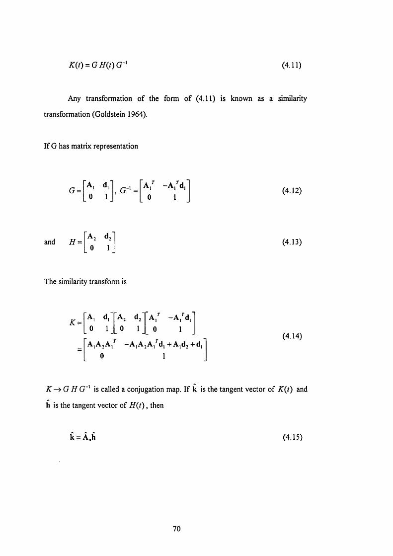
K ( J ) ^ G H { t ) G -1 (4.11)
Any transformation of the form of (4.11) is known as a similarity
transformation (Goldstein 1964).
If G has matrix representation
G =A, d, 'a , -A,^d,’
, G“‘ =0 1 0 1
(4.12)
and H =A j d ;
0 1(4.13)
The similarity transform is
K = ^ iT ^ 2 ^2 0 1 0 1
A / - A / d ,
0 1
AjAjA,^ —A] AjAj^d, + Ajdj + d, 0 1
(4.14)
K - ^ G H G ' is called a conjugation map. If k is the tangent vector of K{t) and
h is the tangent vector of H{t) , then
k = À.h (4.15)
70
where Â* e |/* : T^M ^ 7}^ ) M } is the differential of the conjugation map
at the identity.
A d ' LwJ V A^ - A ^ d 'k =
0 1 - 0 0 0 1
ALw JA ^ -A L w Jd + Av
0 0
(4.16)
Using the identities
1. A[_wJ A ^ = [ A wJ (see A2.1) (4.17)
2. - [A w Jd = |_djAw (by inspection) UL18)
[A w J [d jA w + Av
0 0t U 9 )
Expressed as a six vector
k =Aw
[d jA w + A v04 20)
71
Re-arranging to produce an operator form
k =A 0 I w
[djA A 1 VI:] (4.21)
So A. =A 0
_[djA A(4.22)
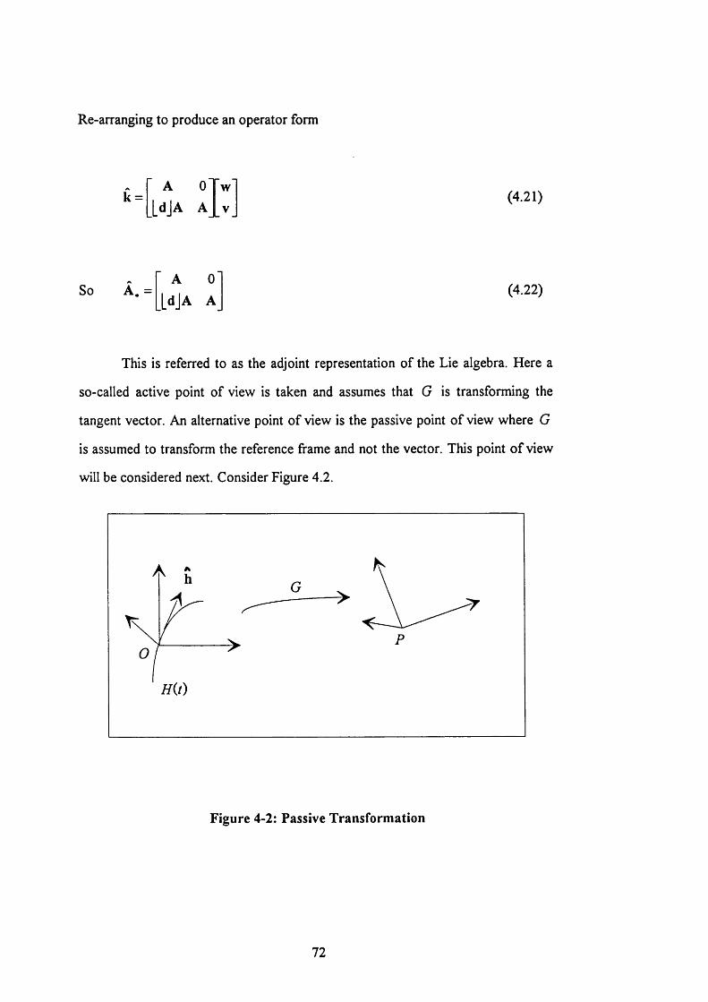
This is referred to as the adjoint representation o f the Lie algebra. Here a
so-called active point o f view is taken and assumes that G is transforming the
tangent vector. An alternative point o f view is the passive point o f view where G
is assumed to transform the reference frame and not the vector. This point o f view
will be considered next. Consider Figure 4.2.
H{t)
Figure 4-2: Passive Transformation
72
The tangent vector h represented in reference frame O becomes
hp = A,
when represented in reference frame P . Now
04.23)
' a '' o ' A O' A 'A 0-A 'LdJ A’’__[djA A -A''[djA + A’"[djA A''A
= I (4.24)
Therefore,
-1A* =A
T 0125)
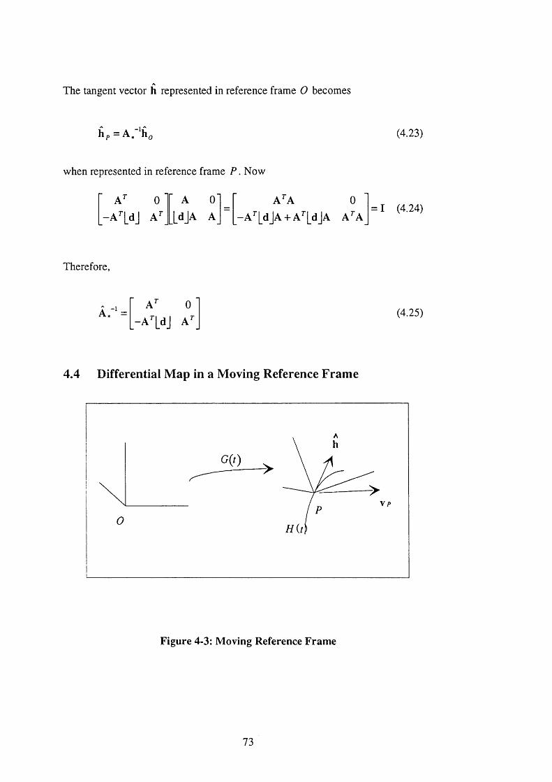
4.4 Differential Map in a Moving Reference Frame
G{t)
\ p
H i t
Figure 4-3: Moving Reference Frame
73
Consider Figure 4-3 where v is the velocity of frame P with respect to
inertial frame O. The derivative of a moving tangent vector is formed by
transforming the tangent vector to the inertial frame, differentiating, and then
transforming back to the moving frame.
d ' J d ' ,(4.26)
where — denotes absolute differentiation and denotes apparent or dt dt
component-wise differentiation (Featherstone 1987).
dtA . =
004.27)
Using the identities
1. 4 “ A = L w JAdt
(see A2.2) 0128)
2. — LdjA = |_V() JA 4- Lw_LdjA (see A2.3) (4.29)
74
dtA , =
[ w JA 0
. [v o jA + fw JL djA |_wjA
M 0
LvoJ L^J.
A o' [djA A
(4 .3 0 )
The differential map operator is denoted ad* . Therefore
a d ^ =[w j 0
_L'’oJ L "J.(4.31)
Therefore
— h = — h + A ,"*ad-°A ,h dt dt *
0132)
4.5 Lie Bracket
It can be shown that ad^ is given by the Lie Bracket (Price 1977).
[81. 82]=[w J V, [WjJ Vj Vj L^iJ V , '
0 0 0 0 0 0 0 0(4.33)
Using the identity (by inspection)
1. (4.34)
75
Therefore
[ i l . §2]=[ [ w j w j [ w . J v , - [ w j j v ,
0 0(4.35)
or represented as a six vector and using the identity (by inspection)
- L '^ 2 j ' 'l= L '’lV 2 (4,36)
we have
[ii .§ 2 ]=
or[81.82]=
L ' ^ l J ' ^ 2
I ' ' lJw 2 -[W l > 2 .
[w i j 0 w .
. b J L ' ^ i J .
= ad j(g ,X g ,)
4.6 Exponential Map
6L37)
0L38)
The following differential equation holds for inertial velocity representation:
G =■[wJ V A d '
_ 0 0 0 1= gC(r) 0L39)
76
The solution is
G (0 = ex p (/g ) (4.40)
which assumes that the fixed and moving frames coincide at the instant
f = 0 . i.e G(0) = I . Therefore a chart in the neighbourhood o f the identity in
S E (3) can be obtained from a basis in jg(3) through the exponential map:
EXP: s e (3 ) - ^S E {3 )
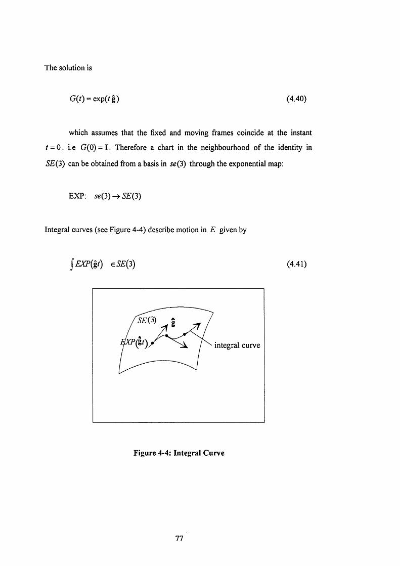
Integral curves (see Figure 4-4) describe motion in E given by
s5 £ (3 ) (4.41)
integral curve
Figure 4-4: Integral Curve
77
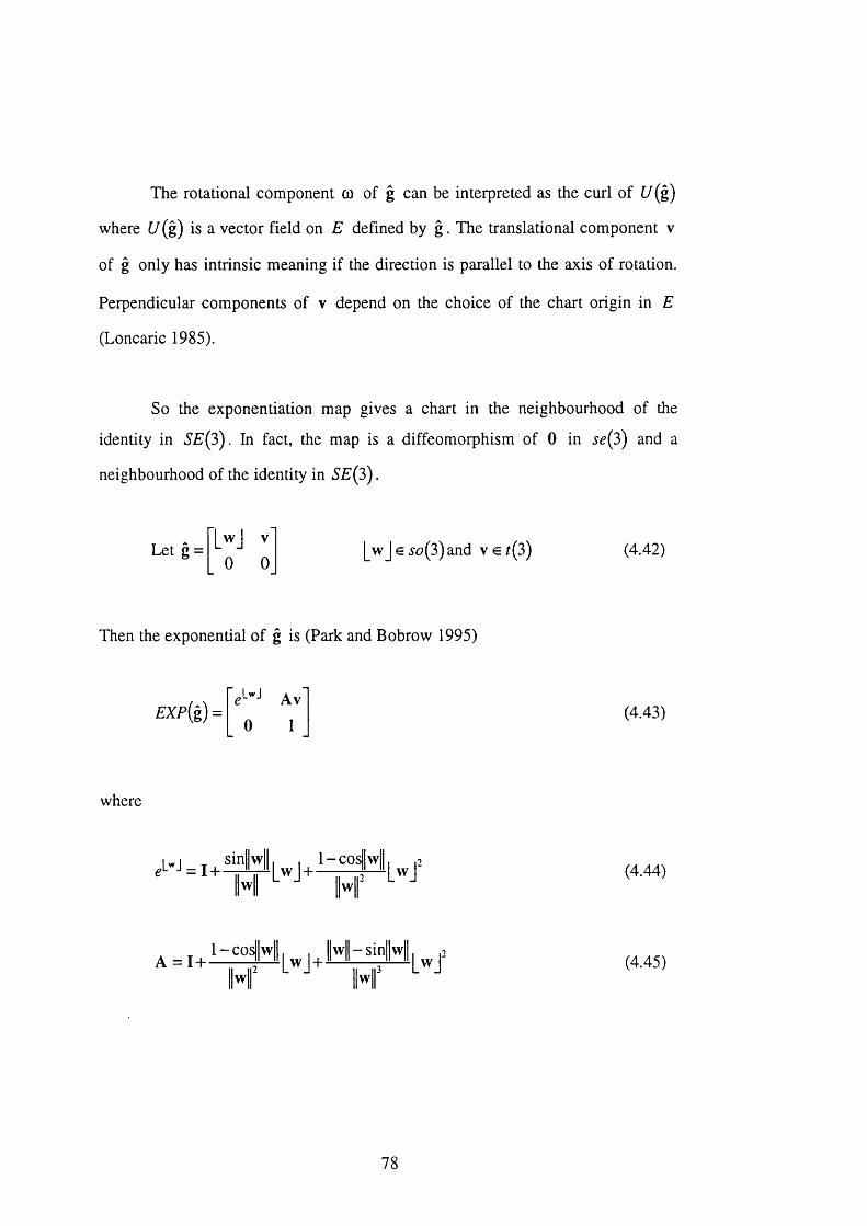
The rotational component CO of g can be interpreted as the curl of U (g)
where U (g) is a vector field on E defined by g . The translational component v
of g only has intrinsic meaning if the direction is parallel to the axis of rotation.
Perpendicular components of v depend on the choice of the chart origin in E
(Loncaric 1985).
So the exponentiation map gives a chart in the neighbourhood of the
identity in SE(3). In fact, the map is a diffeomorphism of 0 in 5^(3) and a
neighbourhood of the identity in S E (3).
Let g =■[wJ v'
0 0|_wj G so(3) and v e r(3) 0L42)
Then the exponential of g is (Park and Bobrow 1995)
£X P(g) =Av'
0 1(4.43)
where
(4.44)
w w04.45)
78
and
»2 2 2 2= 6); +Û)2 (4.46)
Matrix representations can be derived easily. For example, g .S0(3)
with |w | = 1 can be expressed as follows (see A2.4 for proof):
,L"*J _co\v + c
WzV + C û J j û J j V - c y j j
CÛ^CÛ{\f-CÛ2S + W 3V + C
(4.47)
where s = s i n ( ^ ) , c = c o s (^ ) and v = 1 - co s(^ ) .
If we let (0) represent the initial configuration o f a rigid body relative to
a frame A , then the final configuration still with respect to frame A is given by:
(4.48)
Thus the exponential map gives a relative motion o f a rigid body.
The exponential map is extremely important in the geometry o f robotics
and manipulation. An example o f how it can be used is given in the next section.
79
4.7 The Product of Exponentials Formula
The product of exponentials formula gives an expression for the forward
kinematics map of an open-chain robot in terms of relative transformations
between adjacent link frames.
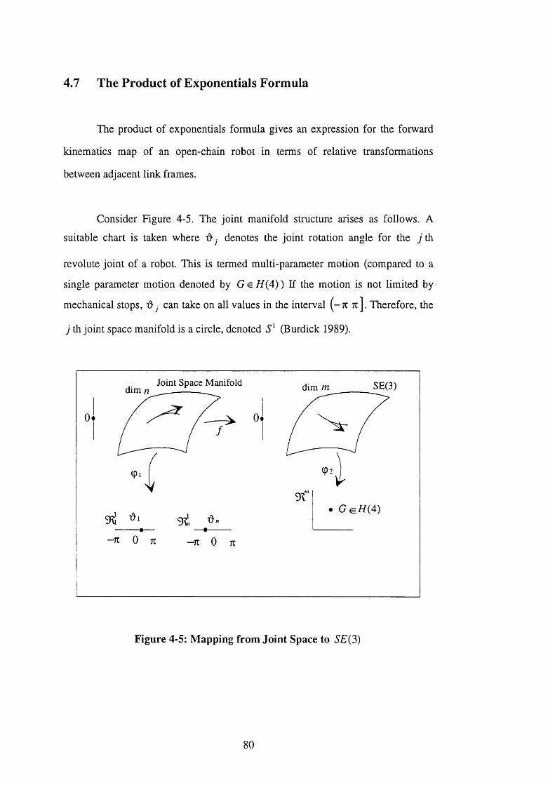
Consider Figure 4-5. The joint manifold structure arises as follows. A
suitable chart is taken where û j denotes the joint rotation angle for the j th
revolute joint of a robot. This is termed multi-parameter motion (compared to a
single parameter motion denoted by G € H{4) ) If the motion is not limited by
mechanical stops, can take on all values in the interval (- tc tt] . Therefore, the
j th joint space manifold is a circle, denoted (Burdick 1989).
Joint Space Manifold SE(3)dim mdim n
Figure 4-5: Mapping from Joint Space to SE(3)
80
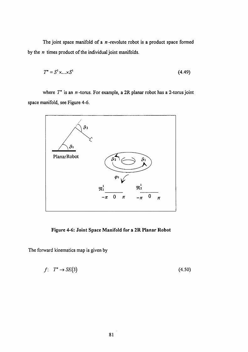
The joint space manifold o f a « -revolute robot is a product space formed
by the n times product o f the individual joint manifolds.
r = a 'x . . .x 3 ' (4.49)
where 7 ” is an n -torus. For example, a 2R planar robot has a 2-torus joint
space manifold, see Figure 4-6.
PlanarRobot
- T V
Figure 4-6: Joint Space Manifold for a 2R Planar Robot
The forward kinematics map is given by
/ : r ^ 5 £ ( 3 ) (4.50)
81
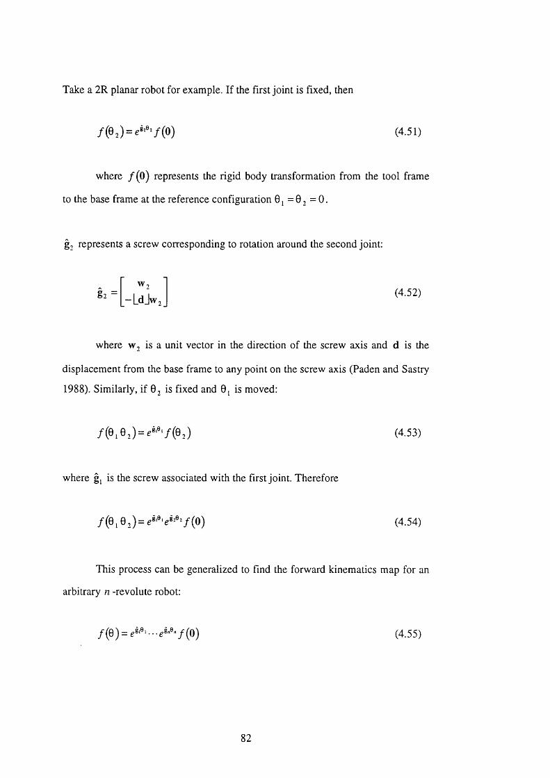
Take a 2R planar robot for example. If the first joint is fixed, then
(4.51)
where /(O ) represents the rigid body transformation from the tool frame
to the base frame at the reference configuration 0 j = 0 , = 0.
§2 represents a screw corresponding to rotation around the second joint:
§ 2 =^2
-L d jw .0L52)
where w , is a unit vector in the direction of the screw axis and d is the
displacement from the base frame to any point on the screw axis (Paden and S as try
1988). Similarly, if 0 , is fixed and 0j is moved:
(4.53)
where gj is the screw associated with the first joint. Therefore
0L54)
This process can be generalized to find the forward kinematics map for an
arbitrary n -revolute robot:
(4.55)
82
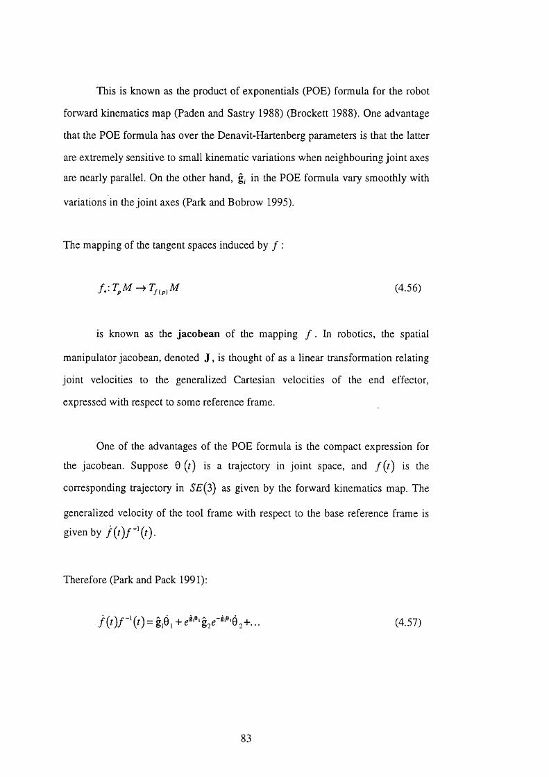
This is known as the product of exponentials (POE) formula for the robot
forward kinematics map (Paden and Sastry 1988) (Brockett 1988). One advantage
that the POE formula has over the Denavit-Hartenberg parameters is that the latter
are extremely sensitive to small kinematic variations when neighbouring jo in t axes
are nearly parallel. On the other hand, g- in the POE formula vary smoothly with
variations in the joint axes (Park and Bobrow 1995).
The mapping of the tangent spaces induced by / :
(4.56)
is known as the Jacobean of the mapping / . In robotics, the spatial
manipulator jacobean, denoted J , is thought of as a linear transformation relating
joint velocities to the generalized Cartesian velocities of the end effector,
expressed with respect to some reference frame.
One of the advantages of the POE formula is the compact expression for
the jacobean. Suppose 0 (t) is a trajectory in joint space, and f ( t ) is the
corresponding trajectory in SE(3) as given by the forward kinematics map. The
generalized velocity of the tool frame with respect to the base reference frame is
given by
Therefore (Park and Pack 1991):
(0 = 1 + ,+ .. . (4.57)
83
This can be expressed in conventional matrix representation, since
is a matrix in 5^(3) and the right hand side can be re-arranged as a
linear transformation o f the joint velocity vector ^he 6 x « matrix
j ( 0 ) .
N ow we have a sensible notation, we can go on to examine the issues o f
shared control. An important issue is the use o f metrics on vector spaces. This will
be examined in the next chapter.
84
Chapter 5
Riemannian Metrics
5.1 Overview of the Chapter
In this chapter, the crucial concept o f Riemannian metrics is examined and
shown to be a generalization o f the inner product at each point on a manifold.
Metrics will be used in the next chapter in the derivation o f filters for shared
control. A metric that is invariant to changes in reference frame is defined as an A ,
- invariant metric. The general form o f the  , - invariant metric for rigid bodies is
derived. An important left invariant Riemannian metric is examined - the kinetic
energy metric.
5.2 Dual Vector
Before metrics can be examined, some further concepts are required. Let
V = V («,K ) be a vector space with basis e ,...e„ . In simple linear algebra, a dual
vector space V*(a2,K ) has a basis such that
e*' (e ,) = 5' (5.1)
85
, fl i f i = jwhere
[O y /
is known as the Kronecker delta. In the context o f manifolds, since T^M is
a vector space, there exists a dual vector space to T ^ M , whose element is a linear
function from T^M to 9%. The dual space is called the co tangent space at p ,
denoted T * M .
Definition 5.1 D ual Vector
An element h ': is called a dual vector or cotangent vector (Nakahara
1990).
Therefore, a dual vector is a linear object that maps a vector to a scalar.
This may be generalized to multilinear objects called tensors, which map several
vectors to a scalar.
Definition 5.2 Tensor F ield
A tensor o f type (g ,r) is a map that maps q dual vectors and r vectors to 91. A
tensor field o f type { q j ) is defined as a smooth assignment o f an element o f the
set o f type (q,r) tensors at each point p e M . A tensor field o f type {q,r) is
denoted
For example, consider a tensor which produces the following mapping at a point:
r^ M -^ 9 1 (5.2)
86
In this case, the tensor must be a dual vector.
Consider a tensor which produces the following mapping at a point:
(5.3)
In this case, the tensor must be a vector.
5.3 Riemannian Metric
A Riemannian metric on a manifold is a smooth assignment of an inner
product to the tangent space at each point on the manifold (Park and Brockett
1994).
Definition 5.3 Riemannian Metric
Let M be a manifold. A R iem annian m etric ^ on M is a type (0,2) tensor field
on M which satisfies the following axioms at each point p e M :
(i) g , ( h .k ) = g , ( k ,h ) h , k e T ^ M (5.4)
(ii) (5 5)
where the equality of (5.5) holds only when h = 0.
Here gp = g\^. gp is a symmetric positive definite bilinear form (Nakahara
1990). If a manifold M admits a Riemannian metric g , the pair ( M, g ) is called
a Riemannian manifold.
87
There exists an isomorphism between T^M and T ^M but no natural
isomorphism. A metric gives a distinguished isomorphism:
g^-.T^M-^T;M (5.6)
h i-> ^,(h, ) (5.7)
Definition 5.4 Inner Product
An inner p roduct, denoted ( , ) is defined as
^h,k^ = g-^(h,k) h,k (5.8)
where g’ (h, j is associated with a mapping to the cotangent space.
Given a basis for the tangent space, an inner product can be written in
terms o f matrices:
(h,k) = h’'Q k (5.9)
where Q is a symmetric matrix. Non-degeneracy o f the inner product is
equivalent to the condition that
d e t(Q )# 0 (5.10)
N ote that if Q is positive-definite, then an associated norm can be defined.
88
5.4 Isometry
The term isometry has been used without proper definition. First some
preliminaries.
A smooth map f \ M - ^ N which induces a differential map / , :
(5.11)
also induces a map / * :
r : T ^ , ^ N ^ T ; M (5.12)
called the pullback map.
Definition 5.5 Isometry
Let { M , g ) be a Riemannian manifold. A diffeomorphism is an
isom etry if it preserves the metric
f ' S n p ) = Sp (5.13)
i e g ^ /( ,) ( / .h , / .k ) = g , ( h ,k ) h , k e 7 ) M (5.14)
I f the metric induced by the left invariant form is the same as that induced
by the right invariant form, the metric is said to be invariant (Price 1977). From
Section 4.2, S E (3) does not have identical left and right invariant forms and
89
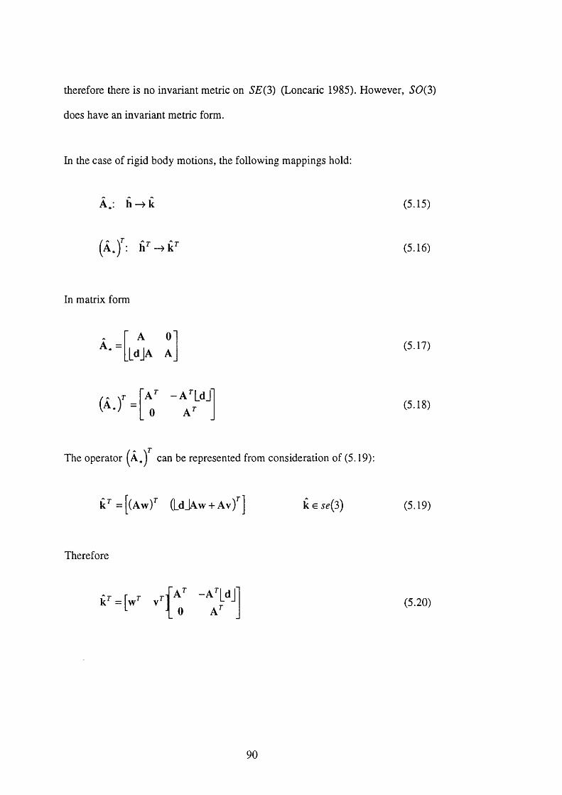
therefore there is no invariant metric on SE(3) (Loncaric 1985). However, S0(3)
does have an invariant metric form.
In the case of rigid body motions, the following mappings hold:
A .: h —> k (5^5 )
(5.16)
In matrix form
A. =A 0
[djA A(5^7 )
( Â . r =A’’ -A^'LdJ 0 A^
(5.18)
The operator can be represented from consideration of (5.19):
k^ = [(Aw)^ (LdJAw + Av)^ k g se(3) (5T9)
Therefore
k ^ = [ w ’'I { 0 A
(5.20)
90
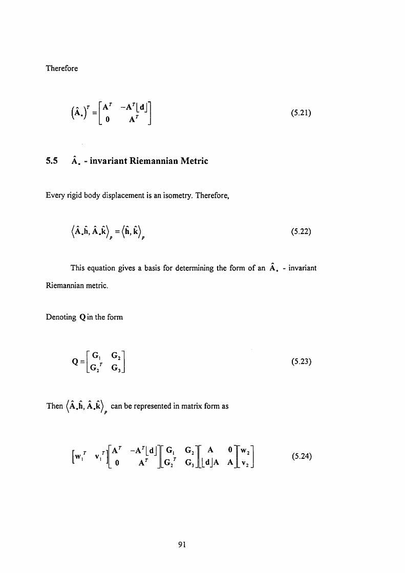
Therefore
(Â ./=A" -A"[dj' 0 A^
(5.21)
5.5 Â, - invariant Riemannian Metric
Every rigid body displacement is an isometry. Therefore,
^ /s \ / a a V(A.h,A.k) = (h ,k ) (5.22)
This equation gives a basis for determining the form of an A, - invariant
Riemannian metric.
Denoting Q in the form
Q =G, G2
G3(5.23)
Then ^A.h, Â,k^ can be represented in matrix form as
[ w ; v / ]A" -A'-[dj' G, G, A o'0 A'' G / G,_ [djA A
(5,24)
91
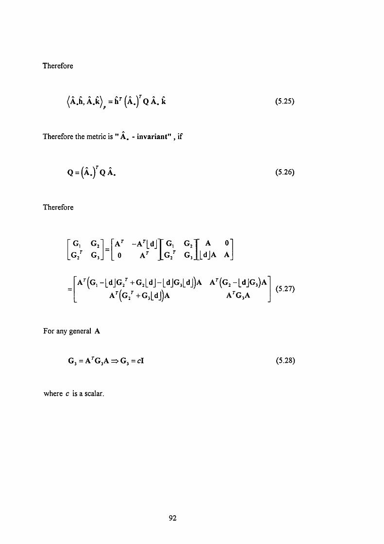
Therefore
^ A \ A — Z a XT " A ^
(A .h ,A .k) = h (a .) Q A . k (5.25)
Therefore the metric is ” A, - invariant” , if
Q = (Â .) Q Â . (5.26)
Therefore
G , G j A ^ “ A ^ l_ d jT G , G j A O'
G / G ,_ 0 A ' X G i ' G , [ d j A A
A^(Gi - [d j G / + G;|_dj - [djGg^dj)A A^(G; -[djG^^A
A ’'( G /+ G 3 [ d j ) A A ’'G jA(5.27)
For any general A
Gj = A GgA Gj = cl (5.28)
where c is a scalar.
92
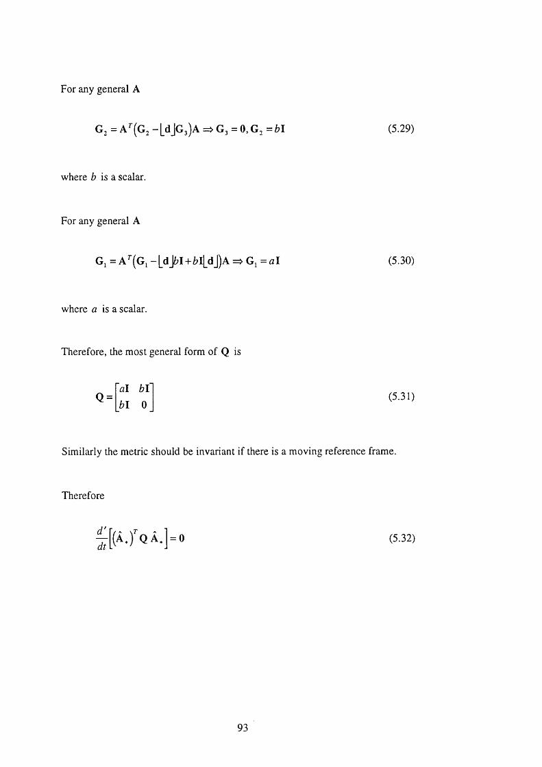
For any general A
G j = A ''(G2 - [ d jG jA => G j = 0, G , = b l (5.29)
where ^ is a scalar.
For any general A
G, = A ''(G , -[d > I+ fc ll_ d J )A => G, = a l (5.30)
where a is a scalar.
Therefore, the most general form of Q is
Q =a l b l
b l 0(5.31)
Similarly the metric should be invariant if there is a moving reference frame.
Therefore
dt[ ( Â . f o A . = 0 (5.32)
93
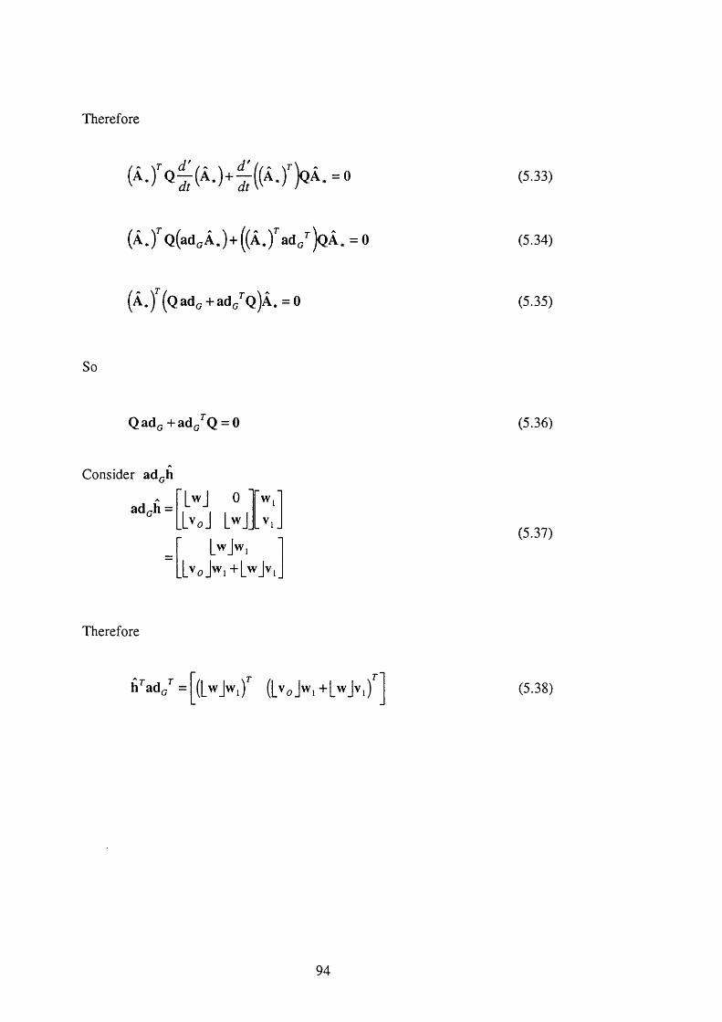
Therefore
(5.33)
(  .) ' 'Q ( a d o  ,) + ( (  .f a d / ) Q  . = 0 (5.34)
(Â*) ( Q a d c + a d /Q ) A , = 0 (5.35)
So
Q a d g + a d g Q = 0 C5 36)
Consider ad^h
ad^h =w,[ w J 0
T o J L'^J
[ w j w , l v o J w , + [ w J v
(5.37)
Therefore
h^adc^ = ( W 'V i f ( h o > i + W v i ) (5 38)
94
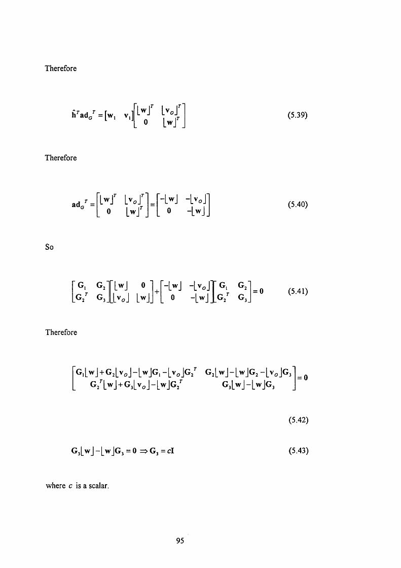
Therefore
h ’' a d / = [w, V,] L - J ' LvoJ^' 0 Lw J'
(5.39)
Therefore
a d / =- [w J -[VoJ
. 0 L w / . _ 0 - [w j_(5.40)
So
G, G / ■[wJ 0 ' - [w J - [ v o j T G, G /G / G,_ I ' ' o J [w j_ 0 “ L '^ J I g / G j
= 0 (5.41)
Therefore
G,LwJ + G2[voJ-LwJG, - [ vqJGj GjLwJ-LwJGj - [ vqJGj= 0
G 3[w J - [ w j G j = 0 G j = c l
(5.42)
(5.43)
where c is a scalar.
95
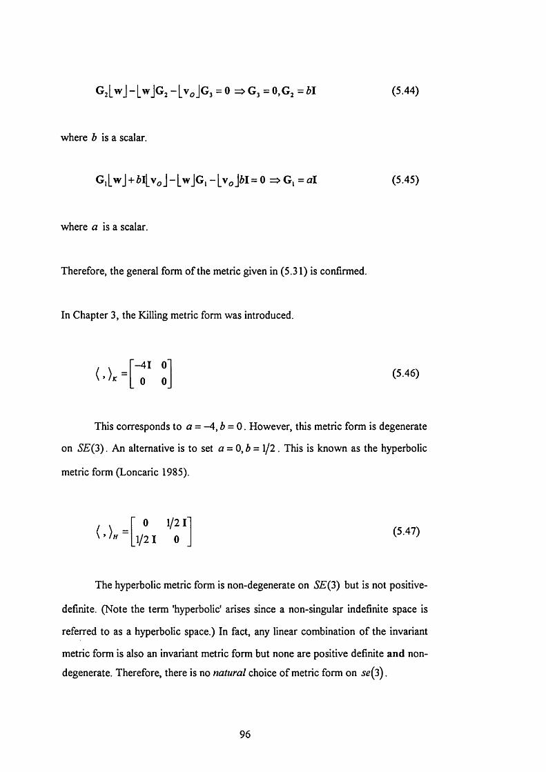
® 2 W - L " 'J g 2 - L '’oJ g 3 = 0 =>G3 = o,G j = h (5.44)
where 6 is a scalar.
G , [ w J + i l [ Vq J - L w JG , - [ Vg J i l = 0 = . G , = a l (5.45)
where a is a scalar.
Therefore, the general form o f the metric given in (5.31) is confirmed.
In Chapter 3, the Killing metric form was introduced.
-4 1 0
0 0(5.46)
This corresponds to a = - 4 ,6 = 0 . However, this metric form is degenerate
on SE (3 ) . An alternative is to set a = 0 ,6 = 1/2. This is known as the hyperbolic
metric form (Loncaric 1985).
( ' ) * -0 1/21
1/21 0(5.47)
The hyperbolic metric form is non-degenerate on S E (3) but is not positive-
definite. (Note the term 'hyperbolic' arises since a non-singular indefinite space is
referred to as a hyperbolic space.) In fact, any linear combination o f the invariant
metric form is also an invariant metric form but none are positive definite and non
degenerate. Therefore, there is no natural choice o f metric form on jg (3 ).
96
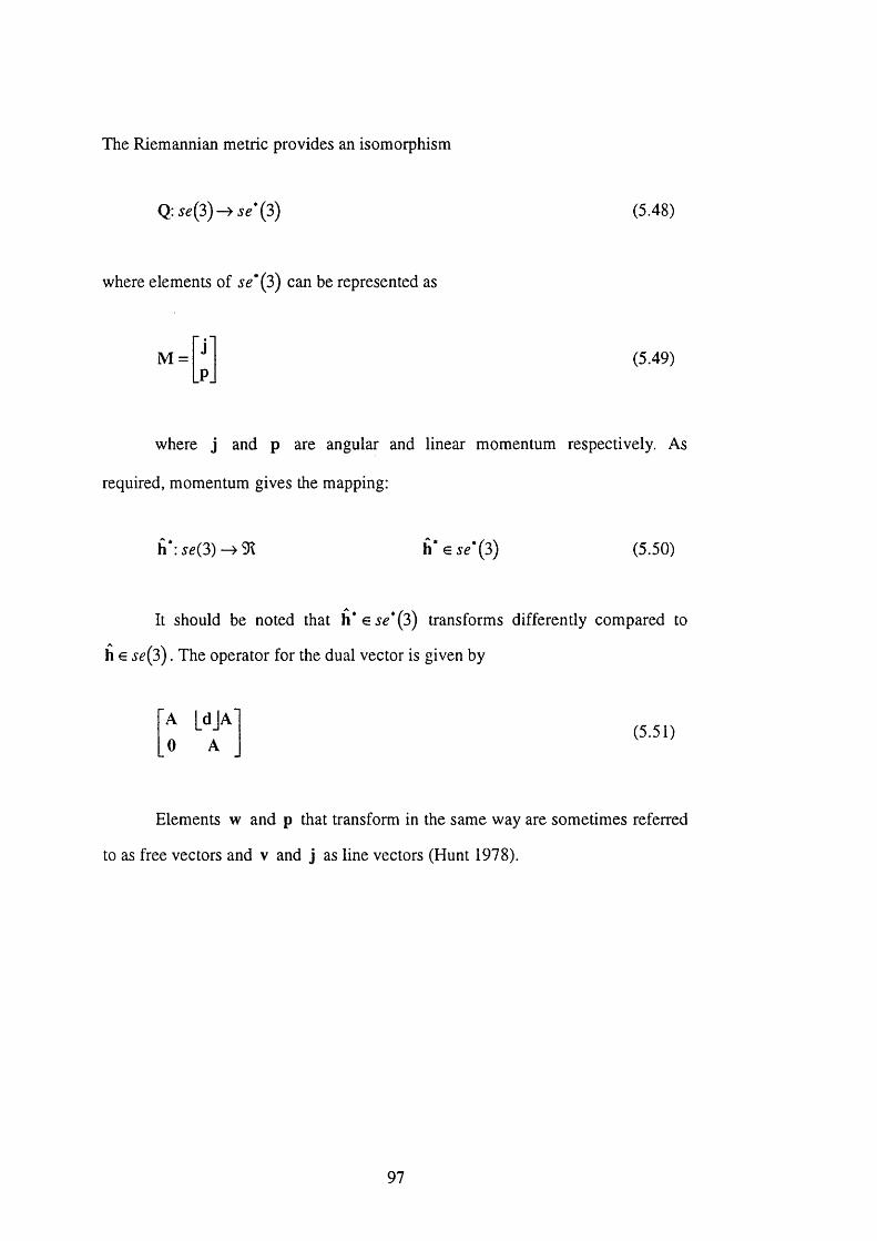
The Riemannian metric provides an isomorphism
Q: s e { 3 ) ^ se*(3) (5.48)
where elements of ^g*(3) can be represented as
M = (5.49)
where j and p are angular and linear momentum respectively. As
required, momentum gives the mapping:
h*: jg(3) —> 91 h* G 5e*(3) (5.50)
It should be noted that h* e jg*(3) transforms differently compared to
h G jg (3 ). The operator for the dual vector is given by
A |_djA
0 A(5.51)
Elements w and p that transform in the same way are sometimes referred
to as free vectors and v and j as line vectors (Hunt 1978).
97
5.6 Kinetic Energy Metric
The kinetic energy of a rigid body is a left invariant Riemannian metric
associated with a left invariant tangent vector (Arnold 1978), denoted
Before the metric can be examined, a definition is required:
Definition 5.6 Kinetic Energy
Let M be a Riemannian manifold. The quadratic form on each tangent space
K = \/2 { y ,v ) x e s e { 3 ) (5.52)
is called the kinetic energy (Arnold 1978).
The kinetic energy of a rigid body at the centre of mass is given by
= l/2 (w ^ n „ ,w + m v^v) (5.53)
where m is the mass of the rigid body and is the inertia tensor of the
rigid body about the centre of mass, relative to a frame at the centre of mass.
Therefore
= l/2 [w " v T '0 m l
w
v(5.54)
9 8
Therefore
i^ = l/2 h ^ Q h (5 55)
where the generalized moment of inertia, is given by
Q ' =K O '
0 m l(5.56)
The same body has a more complicated generalized moment of inertia
when viewed from another frame (Selig 1989). In particular, if y is x translated by
t, the off-diagonal blocks of Q are antisymmetric matrices:
Q ' = (5^7 )
The generalized moment of inertia is not an A , - invariant metric as
defined in Section 5.5; the matrix Q needs to be transformed with a shift in the
measurement frame:
(5JW)
99
5.7 Orthogonality and Reciprocity
'Strict' orthogonality is only defined on a Euclidean metric space, E " . I f
a b = 0 a . b e E " (5.59)
where • denotes dot product, then a and b are orthogonal.
However, invariant 'notional' orthogonality, or reciprocity, can be defined
for elements in the Lie algebra o f 5E(3) using the hyperbolic metric. If
h ^ Q k = 0 h , k G ^ 3 ) (5.60)
where Q is ( , ) ^ , then h and k are reciprocal.
I f 2 ( , is used in (5.60) then the equation is referred to as a reciprocal
product. A reciprocal product between a tangent vector and a dual vector is given
in matrix form by:
(h*) k = 0 h* EJg"(3), k € Jg(3) (5.61)
I f (5.61) holds then then h* and k are reciprocal.
100
5.8 Validation of the Reciprocal Product
A simple check is made to show that the reciprocal product is invariant to
changes in measurement frame.
I f two elements o f se(3) are reciprocal via then under a change o f
reference frame, the reciprocal product becomes:
' a ’' -A ''[djT o r A O ' w
0 A '' J [ l 0 [djA A v(5.62)
Simplifying
■A’'[d jA + A ''[d jA A ’'a '
A ’'A 0
w
V(5.63)
which gives
"0 r w
1 0 v(5,64)
Therefore, under a change o f reference frame, the two elements will still be
reciprocal.
101
Similarly it can be easily shown that reciprocity between a tangent vector
and a dual vector is invariant to changes in reference frame. I f an element o f je(3)
is reciprocal to an element o f , then under a change o f reference frame, the
reciprocal product becomes
[ j- p ' l■ A' 0 ' A O' w
- A ^ d J A'"_ _[djA A V(i.65 )
Simplifying
[ i ' p ’ lA'^A
_-A’'[djA + A''[djA A’'Aw
V(5,66)
which gives
[1’ p’ lw
V(5.67)
Therefore, under a change o f reference frame, the two elements will still be
reciprocal.
102
Chapter 6
Invariant Filtering for Shared Control
6.1 Overview of the Chapter
In this Chapter, a proper framework is outlined for implementing shared
control in a geometrically correct way. A simple partitioning o f je(3) is considered
first. Traditionally this has been done using a switching matrix. This is shown to be
equivalent to a filter which embodies the metric form { , ) j . I f the filter is to be
successful when the reference frame is moved, then the metric form has to be
transformed correctly.
The case o f shared control with constrained motion is considered next. The
critical relationship in this case is shown to be the reciprocal product between
elements o f 5^(3) and Jg '(3 ) .
The switching matrix is re-examined next and shown to be a
misinterpretation o f a projection operator which is a proper geometric entity. The
necessary transformations for the use o f the projection operator are derived.
103
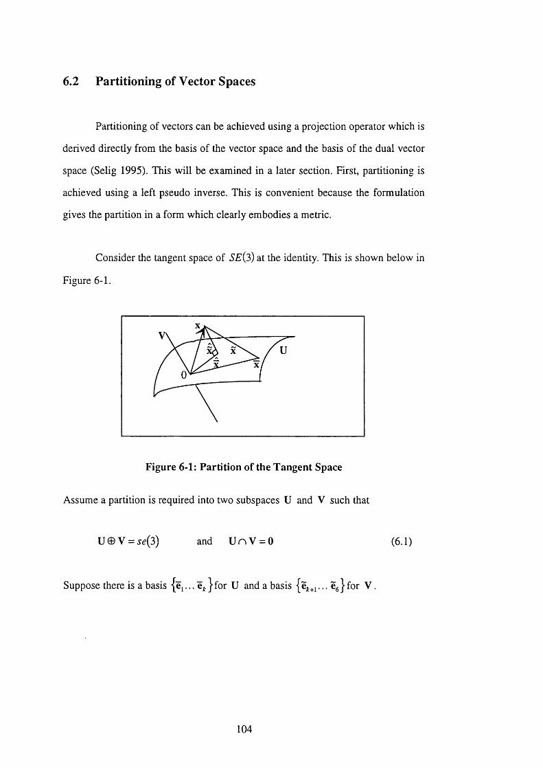
6.2 Partitioning of Vector Spaces
Partitioning of vectors can be achieved using a projection operator which is
derived directly from the basis of the vector space and the basis of the dual vector
space (Selig 1995). This will be examined in a later section. First, partitioning is
achieved using a left pseudo inverse. This is convenient because the formulation
gives the partition in a form which clearly embodies a metric.
Consider the tangent space of SE{3) at the identity. This is shown below in
Figure 6-1.
Figure 6-1: Partition of the Tangent Space
Assume a partition is required into two subspaces U and V such that
U e V = jg(3) and U n V = 0 (6.1)
Suppose there is a basis {e^... e ^ jfo r U and a basis {e^+^... e^} for V
104
Now consider a vector x e ^g(3). It is always possible to write
x - a ^ t y + +a^e^ (6.2)
Let My be the matrix whose columns are e^.}, so that
X = (6.3)
where
a,
(6.4)
This follows since
M u a ,= [ e , ... e* (6.5)
or
M^a^. = a^e^+...+af.e^ (a. are scalars) (6 .6)
With reference to Figure 6-1, x can be viewed as the vector sum of a
unique x e U and x e V , or as the vector sum of a general x e U and x ë V .
Note that x is a minimum x on V .
105
Define an error term, e , where
\\ef =||M ^ja^ -xll" (6.7)
if X e U , then
INI' = IlM^ak - xll
= 0
More generally,
||e f = ||M jjâ k - x | |“ > 0 (6.8)
In Section 6.3, for an equation of the form
M jjâ^ = X (6.9)
where has full column rank, the error term is shown to be minimized
in a least squares sense by a choice of , denoted , where
t , = M / x (6.10)
where denotes the left-pseudo inverse of . The matrix M^. has
full column rank since its columns are basis vectors of U . Re-call that
x = (6.11)
106
Therefore
x = M jjâ , (6.12)
Substituting (6.10) into (6.12) gives
^ = (6.13)
An similar argument follows for x giving
X = M v M v ^ x (6.14)
Now
x = x + x (6.15)
Therefore
X = MyMjj'^x + MylVIy'^x (6.16)
6.3 Left Pseudo-Inverse
For partitioning a real vector space, an explicit formula is required for left
pseudo-inverse in (6.10). It is shown in this section that the solution requires a
choice of metric.
107
A formula for left pseudo inverse arises from consideration of an ordinary
least squares problem. An ordinary least squares problem is characterized by
Ax = b (6.17)
where A is m x n .
The best choice x is the one that minimizes the norm of the error vector
(Strang 1986), where the error vector is defined as
e = A x - b (6.18)
The norm of the error vector is given by
I Ax - b II = ( A x - b ) ^ Q ( A x - b ) (6.19)
where Q is the matrix form of a Riemannian metric.
Expanding
Ax - b If = (A x)'' Q(Ax) - 2(A x)'' Q b + b'^Qb (6.20)
The term b'^Qb will not affect any minimization and can be ignored.
Define a function
P(x) = l /2 (A x ) ''Q (A x )-(A x ) ''Q b (6.21)
108
Define
M ^A ^'Q A (6.22)
n = A Q b (6.23)
Therefore
P(x) = 1/2 - x ^ n (6.24)
If M is positive definite, then P {\) is minimized at the point
x = M “' n (6.25)
(see A2.5 for proof).
Substituting back
x = (A ’’Q A ) '‘A ''Q b (6.26)
is the least squares solution to (6.17).
109
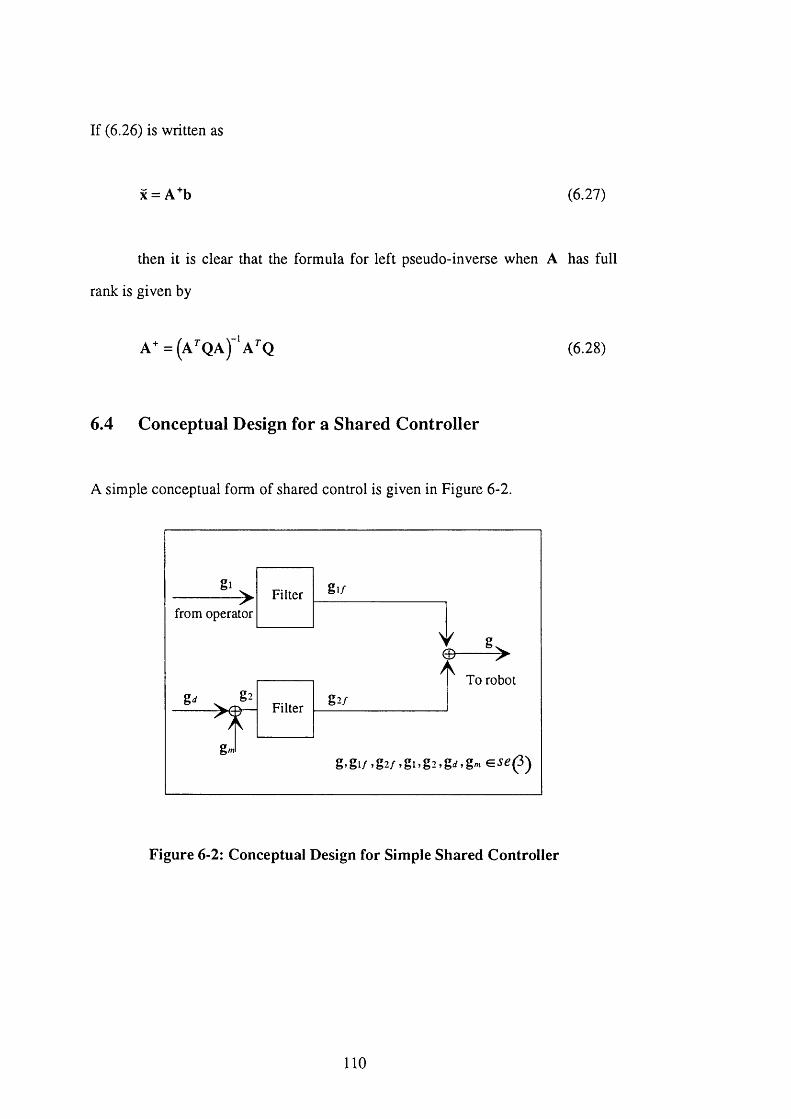
If (6.26) is written as
x = A+b (6 .2 7 )
then it is clear that the formula for left pseudo-inverse when A has full
rank is given by
A^ = (A ^ Q A ) ''a ^Q (6.28)
6.4 Conceptual Design for a Shared Controller
A simple conceptual form of shared control is given in Figure 6-2.
gi/Filterfrom operator
To robot
Filter
g» g l/» g2/> §15 §2 > ^S6
Figure 6-2: Conceptual Design for Simple Shared Controller
110
In this case, there is a simple partition of se(3) such that
U © V = se{3), U n V = 0 (6.29)
From (6.16)
g = M ^ M / g + M ^ M / g (6.30)
If a definition is made
g^ = M u M / g (6.31)
then the formula for left pseudo inverse gives the following expression:
= M „ ( M / Q M „ ) ' ' M / Q g (6.32)
Now a switching matrix is defined as . Therefore, for a switching
matrix
g^ = M , . M / g (6.33)
Comparing (6.32) and (6.33) yields for a switching matrix
(6.34)
This is true in general if Q = I , since
1 1 1
(m / I M „ ) “ M / l = r ‘M / = M / (6.35)
Therefore, it is now possible to conclude that the switching matrix is
associated with ( , where
( ’ }/ -1 O'
0 1(6.36)
6.5 Design for Invariant Filtering
There is no unique way to partition g e se(3) because there is no natural
positive definite metric on se(3) (Loncaric 1985). Any symmetric positive
definite metric can be used but the metric has to be transformed correctly with a
change in reference frame (Lipkin and Duffy 1988) (Doty et al 1993). For
example, if ( , ) is used, then the transformation is
Q - ^ ( Â . f Q Â . = ( Â . ) ' ' Â . (6.37)
6.6 Shared Control and Constrained Motion
To re-cap, a dual vector is a linear function:
(6.38)
Momentum, denoted M , is an element of the cotangent space to the Lie
algebra jg(3), denoted jg* (3).
1 1 2
M = se *(3) (6.39)
where j and p are the angular and linear momentum.
Under a rigid body displacement in SE (3), the momentum will change.
The derivative of the momentum is given by
M =mf
(6.40)
where f denotes linear force and m denotes moment (collectively refened
to as a force vector). This vector will lie in the tangent space to but since
this is a finite dimensional vector space, its tangent space is naturally isomorphic
to the space itself. Hence a force vector is an element of se*(3) (Selig 1995):
mf
G se*{3) (6.41)
This force vector is sometimes referred to as a wrench.
At this point, it should be emphasized that velocities and forces lie in
different (dual) vector spaces. A proper mathematical approach is required for
discussing forces and velocities together in a geometrically correct way. This is
described in the following sections.
113
6.7 Symplectic Vector Space
First some definitions are required.
Definition 6.1 Dual Vector Space
Let M be an « - dimensional manifold. A dual vector on the tangent space
to M at a point p is called the dual vector to M at /?. The set of all dual vectors
to M at p forms an n - dimensional vector space, dual to the tangent space
TpM , called the dual vector space, denoted T^*M .
Definition 6.2 Cotangent Bundle
The union of T j M at all points p e M is called the co tangent bundle of
M and is denoted T*M (Arnold 1978).
The set T* M has a natural structure of a manifold of dimension I n . Now a
choice of chart gives a point in the tangent space a representation p of dimension
n . Similarly the choice of chart gives a point in the dual vector space a
representation q of dimension n . Together the 2n representation (p, q) g 91'"
characterizes T*M (Arnold 1978).
A symplectic linear structure on 91‘" can be defined by a form known as
the skew scalar product. Some definitions are required.
114
Definition 6.3 Skew Scalar Product
A symplectic linear structure on is a non-degenerate bilinear skew symmetric
form, called the skew scalar p roduct, denoted [[ , ]]
]] = -[[^ .n ]] s 9î-”
Definition 6.4 Symplectic Vector Space
The space together with the symplectic structure [ [ , ]] is called a sym plectic
vector space (Arnold 1978).
Definition 6.5 Symplectic Group
A linear transformation 91"" of the symplectic space to itself is
called symplectic if it preserves the skew scalar product
[ [ 5 ^ ,5 t i]] = [[^,T |]] V^,T1 g 'R-"
The set of all symplectic transformations of is called the sym plectic group
Sp{2n). (This group has already been discussed in Section 2.5.)
Definition 6.6 Skew Orthogonal
Two vectors ^,T| e are skew orthogonal if
[R .n ]] = 0
115
Definition 6.7 Langrangian Plane
A k - dimensional plane of a symplectic space is a null (or isotropic) plane if it is
skew orthogonal to itself, i.e. if the skew scalar product of any two vectors in the
plane is equal to zero. If k = n the null plane is called a Lagrangian plane
(Arnold 1978).
In this case, the 12-dimensional representation is given by
(h ,h * )s9 î‘- (6.42)
A partially constrained rigid body can always be characterized by a
Langrangian plane in by encapsulating a reciprocal relationship into the
definition of the skew scalar product :
[ [(h „ h ;) ,(h ,,h ,‘) ]]= h ;h ,-h ,;h , (6 .4 3 )
It is tempting to assert that a partially constrained rigid body can be
characterized by the subspace of h and the subspace of h* which simply sum to
span 91 (Vukobratovic and Stojic 1995). However, from a geometric viewpoint,
this assertion would be incorrect since the two belong to different vector spaces. A
geometrically correct description is as follows: a partially constrained rigid body is
characterized by a Langrangian plane in 91 " where the symplectic structure of
9t^~ is defined by the skew scalar product given in (6.43) (Loncaric 1985).
116
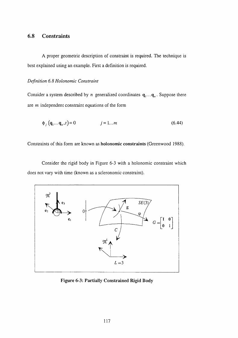
6.8 Constraints
A proper geometric description of constraint is required. The technique is
best explained using an example. First a definition is required.
Definition 6.8 Holonomie Constraint
Consider a system described by n generalized coordinates . Suppose there
are m independent constraint equations of the form
<t>; ( q i - - - q , . 0 = o y = 1... m (6.44)
Constraints of this form are known as holonom ie constra in ts (Greenwood 1988).
Consider the rigid body in Figure 6-3 with a holonomie constraint which
does not vary with time (known as a scleronomic constraint).
G =
L =3
F igure 6-3: Partia lly C onstrained Rigid Body
117
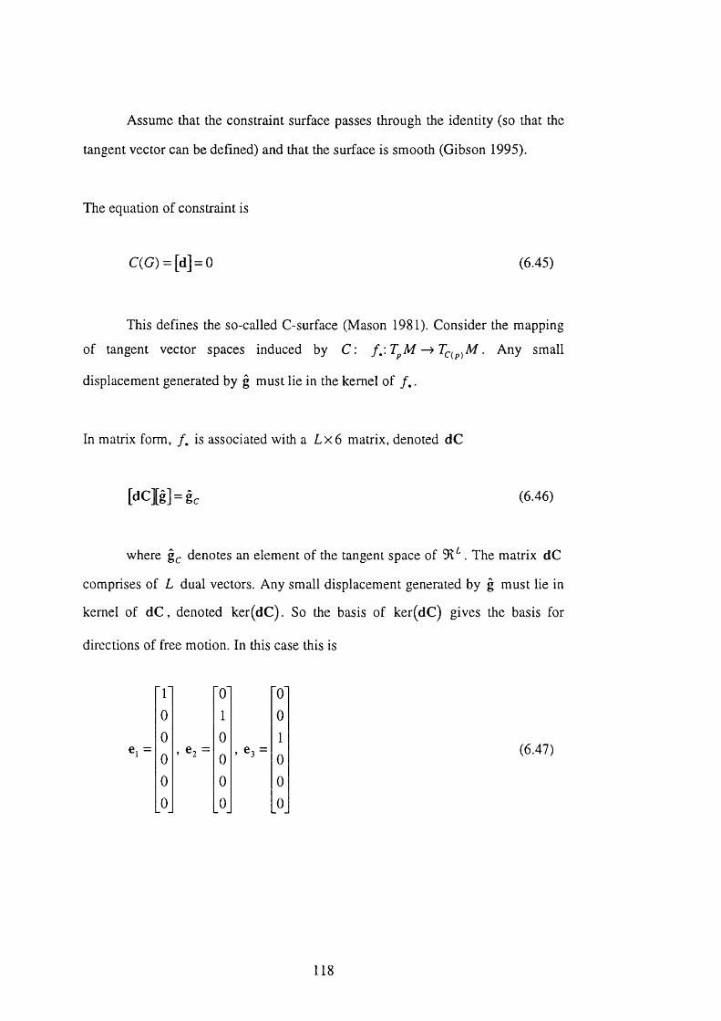
Assume that the constraint surface passes through the identity (so that the
tangent vector can be defined) and that the surface is smooth (Gibson 1995).
The equation of constraint is
C(G) = [d] = 0 (6.45)
This defines the so-called C-surface (Mason 1981). Consider the mapping
of tangent vector spaces induced by C : /*: ^ . Any small
displacement generated by g must lie in the kernel of /* .
In matrix form, / . is associated with a L x 6 matrix, denoted dC
[dC][g] = g , (6.46)
where g . denotes an element of the tangent space of 91^ . The matrix dC
comprises of L dual vectors. Any small displacement generated by g must lie in
kernel of d C , denoted ker(dC ). So the basis of ker(dC) gives the basis for
directions of free motion. In this case this is
e, =
"f "o' " 0"
0 1 00
, G-j —0
, 63 =
10 0 00 0 00 0 0
(6.47)
118
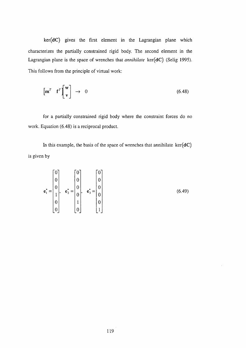
ker(dC ) gives the first element in the Lagrangian plane which
characterizes the partially constrained rigid body. The second element in the
Lagrangian plane is the space of wrenches that annihilate ker(dC ) (Selig 1995).
This follows from the principle of virtual work:
I " ' 0 (6.48)
for a partially constrained rigid body where the constraint forces do no
work. Equation (6.48) is a reciprocal product.
In this example, the basis of the space of wrenches that annihilate ker(dC )
is given by
e , =
"O' "o' "0"
0 0 0
0, 02 =
0, e t =
0
1 0 0
0 1 0
0 0 _1
(6.49)
119
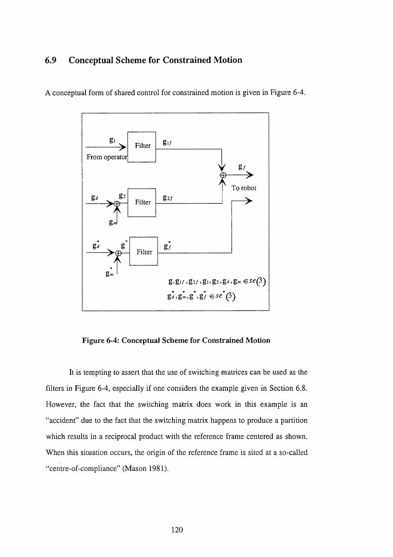
6.9 Conceptual Scheme for Constrained Motion
A conceptual form of shared control for constrained motion is given in Figure 6-4.
gi/
From operator
To robot
Filter
Filter
Filter
g, gi/ , g2/ , gi, g2,grf, gm G Jg(3)
g d , g , n , g , g f G5e"(3)
Figure 6-4: Conceptual Scheme for Constrained Motion
It is tempting to assert that the use of switching matrices can be used as the
filters in Figure 6-4, especially if one considers the example given in Section 6.8.
However, the fact that the switching matrix does work in this example is an
“accident” due to the fact that the switching matrix happens to produce a partition
which results in a reciprocal product with the reference frame centered as shown.
When this situation occurs, the origin of the reference frame is sited at a so-called
“centre-of-compliance” (Mason 1981).
1 2 0
If one considers a shift in the reference frame from this “centre of
compliance”, then the naive use of the switching matrix on the transformed
vectors will not produce correct results. This will be validated in the next section.
If the reference frame is shifted then, using the method outlined in Section
6.5, the respective filters can be transformed so that elements are filtered correctly.
Although jg(3) is isomorphic to 91^, it is not a Euclidean metric space.
Therefore, complements of se(3) can be defined as only locally orthogonal to
each other. Similarly complements of ^e*(3) can be defined as locally orthogonal
to each other. Note that it would be incorrect to assert that complements of jg(3)
and complements of se* (3) are orthogonal to each other because the complements
lie in different vector spaces (Duffy 1990).
6.10 Validation of Invariant Filtering
An example of a shared mode task is examined which involves constrained
motion. Using a test harness, both the filters derived in Section 6.5 and the
switching matrix are tested. The task is the peg in the hole task introduced in
Section 1.3.2. Consider a unit shift in origin in the direction shown in Figure 6-5.
This example is deliberately the same as used in Lipkin and Duffy (1988) in order
to show consistency of results.
121
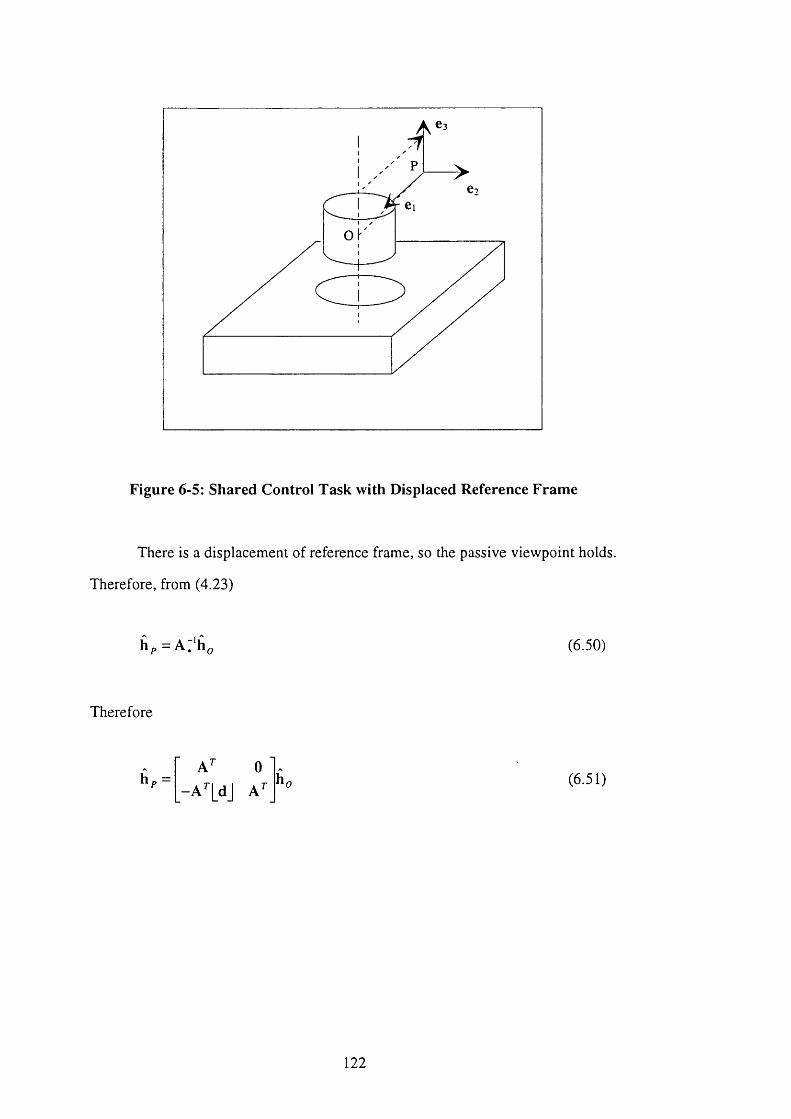
Figure 6-5: Shared Control Task with Displaced Reference Frame
There is a displacement of reference frame, so the passive viewpoint holds.
Therefore, from (4.23)
hp = A :‘h^ (6.50)
Therefore
hp =0
-A"LdJ A"(6.51)
1 2 2
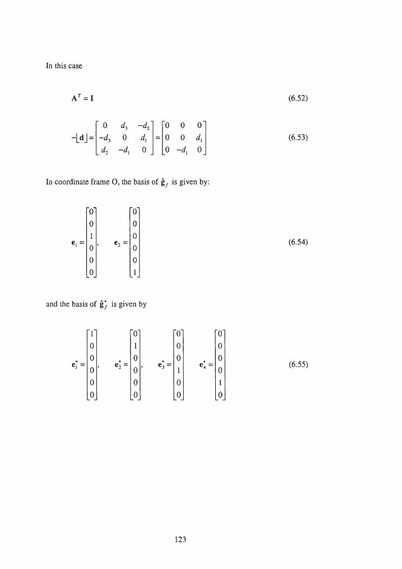
In this case
A^ = I (6.52)
■ 0 4 ~di ' 0 0 O '
L d j = 0 di = 0 0 d:-d, 0 0 -d, 0
(6.53)
In coordinate frame O, the basis of gy is given by:
e, =
'O' 'o'0 0
1-
0
0 0
0 0
0 1
(6.54)
and the basis of gy is given by
e, =
' I ' 'O' O' 'O'
0 1 0 0
0 0 0 0e*2 = Cj = =
0 0 I 0
0 0 0 I
0 0 0 0
(6.55)
123
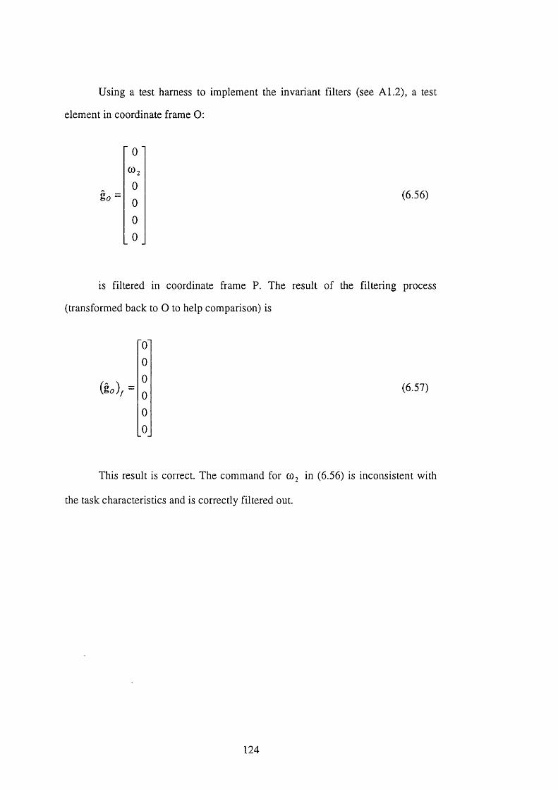
Using a test harness to implement the invariant filters (see A1.2), a test
element in coordinate frame O:
go
0CO20000
(6.56)
is filtered in coordinate frame P. The result of the filtering process
(transformed back to O to help comparison) is
iS o ) , = (6.57)
This result is correct. The command for co, (6.56) is inconsistent with
the task characteristics and is correctly filtered out.
124
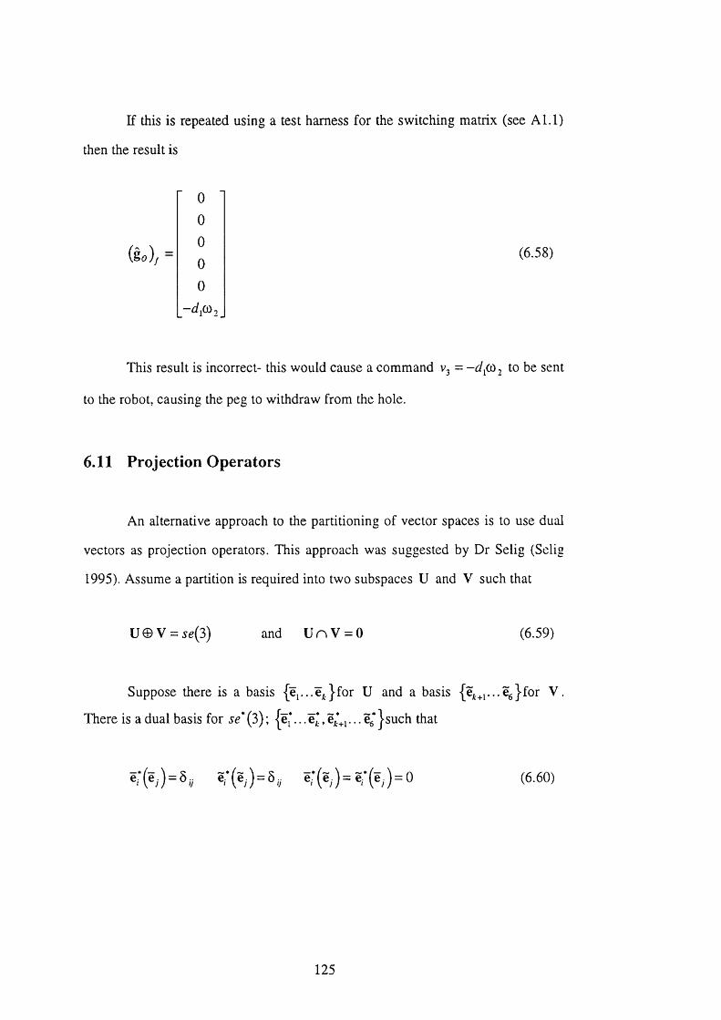
If this is repeated using a test harness for the switching matrix (see A I.l)
then the result is
00000
-d^Cùj
(&58)
This result is incorrect- this would cause a command v. = to be sent
to the robot, causing the peg to withdraw from the hole.
6.11 Projection Operators
An alternative approach to the partitioning of vector spaces is to use dual
vectors as projection operators. This approach was suggested by Dr Selig (Selig
1995). Assume a partition is required into two subspaces U and V such that
U © V = 5^(3) and U V = 0 (6.59)
Suppose there is a basis {ep..e^.}for U and a basis {ê^_^i...êg}for V
There is a dual basis for se*(3); {ë* ...ë^,ë^+ ...% }such that
(6.60)
125
Now consider a vector x e se(3). It is always possible to write
X - . . + a ^ e ^ + . . + « 6 ^ 6 05.61)
where the coefficients are given by;
a, = e*(x) \ > i > k and a- = e,*(x), ' +1 > / > 6 (6.62)
Projection operators can be constructed as follows. Let be the matrix
whose rows are the transpose of Therefore
m ; x =
a,
05 63)
Next let Mjj be the matrix whose columns are {e,...e^.}, so that
(6.64)
So the projection operator which projects vectors onto the subspace U is
given by M ^ M u .
It is straightforward to find projection operators for V , and, by a similar
argument as given above, for U* and V* where
U * ©V * = j ^* ( 3 ) and U * n V * = ( ) 05.65)
126
The square projection operator is a proper geometric entity which can be
misinterpreted as a switching or selection matrix in a particular measurement
frame.
Given this construction, it is simple to see how this projection operator
will transform with a change in reference frame. In frame O,
~ ^ f o (6 .66)
where / denotes filtered. In a new frame P,
=Xyp (6.67)
But (6.67) can be written as
M„pM'„pA:‘xo = Â:'x^„ (6.68)
Therefore
Comparing (6.69) and (6.66),
(6.70)
127
Therefore
This transformation is verified in A 1.3.
6.12 Transformation of Velocity
The mapping of the tangent spaces induced by the forward kinematics map / :
(6.72)
is known as the Jacobean of the mapping / . The spatial manipulator
Jacobean as defined on page 83 is denoted J . For an non-redundant robot
n = m = 6 . In general
g = J 0 (6.73)
Referring to Figure 6-4, if there were no filters present, then the
transfomiation would be expressed as given in (6.73). With a filter F present,
F g = F J 0 (6.74)
Therefore,
0 = ( F j ) * f g (6.75)
128
Therefore
0 = ( f j ) % (6.76)
Early implementations of hybrid position / force control mistakenly
implemented equation (6.76) as
0 = ( F J ) % (6.77)
This was incorrect because in general FJ is a singular matrix and does not
have an inverse. This was first pointed out in Fisher and Mujtaba (1992).
However, their alternative scheme featured a switching matrix and therefore
cannot be considered as a complete and proper description in a geometric sense.
The appearance of the left pseudo inverse of the Jacobean gives the shared
control scheme an analogy with the control of redundant manipulators (Burdick
1989). The general solution of (6.75) for a revolute robot is in fact
0 = ( F j ) l / + [ l - ( f j ) " ( F j ) ] z (6.78)
where z is an arbitrary n x l vector. Following Fisher and M ujtaba (1992),
z is set to zero, and the so-called “minimum norm” solution is used, given in
(6.76).
129
Chapter 7
Compliance and Shared Control
7.1 Overview of the Chapter
The implementation o f an explicit force control scheme is commonly
undertaken by closing a external force control loop around an inner position
control loop. A wrist-mounted force sensor is typically used. It has been
extensively reported that this type o f scheme suffers from instability when
contacting a stiff environment. The destabilizing mechanism is high gain combined
with the use o f a non-collocated sensor (Eppinger and Steering 1987) (Daniel et al
1993). Many robot control architectures preclude the implementation o f robust
force control. However, a compliant device mounted between the robot wrist and
the workpiece can be a good alternative, in lieu o f explicit force control.
In this Chapter, the geometry o f compliant devices is examined in the
context o f shared control. In this form o f shared control, force and displacement
are regulated by control o f displacement only. A geometrically correct scheme for
shared control based on the use o f a compliance is derived. This follows naturally
from a theoretical analysis o f stiffness and potential energy.
130
7.2 Stiffness
A compliant device is referred to as a generalized spring. A generalized
spring is mathematically represented by a potential energy function V defined on
SE(3):
V :S E ( 3 ) - ^ S i (7.1)
For a particle , it is possible to define a force in terms of the gradient on V :
F = -g r a d V (7.2)
Equation (7.2) assumes the existence of a natural positive definite metric.
Since there is no natural positive definite metric on SE{3) , this definition cannot
be used. Instead the force exerted by a generalized spring on the rigid body that the
spring is attached is given by
F = - d V (7.3)
where F e se* {3).
Definition 7.1 Stiffness
At the identity of SF(3), stiffness is a mapping which maps small displacements
into forces:
f : s e (3 ) -^ se * {3 ) (7.4)
131
The required mapping is given by the Hessian d^V at the identity (Loncaric 1985)
Stiffness is defined as
(Note that one can use left translation to move the region o f interest to the
identity.)
Stiffness K can be represented by a symmetric 6 x 6 matrix:
A B
C(7.5)
where A = , C = and B are 3 x 3 matrices (Loncaric 1985).
7.3 Potential Energy
The force resulting from a small displacement is
m A B w
f B^ C v(7.6)
This relationship gives rise to an expression for potential energy stored in a
generalized spring system. First a definition:
132
Definition 7.2 Potential Energy
Let M be a Riemannian manifold. A differentiable function U
(7.7)
is called potential energy (Arnold 1978).
For a generalized spring system, potential energy can be expressed
algebraically as
[ „ ' . ' IA B w
C V>0 (7.8)
For calculation o f potential energy under displacement o f the measurement
reference frame
k ^ ( â . ) ’' k â . (7.9)
This is analogous to the expression for the transformation o f the matrix
associated with the kinetic energy metric. The transformation ensures that the
potential energy measure is invariant to changes in measurement reference frame.
133
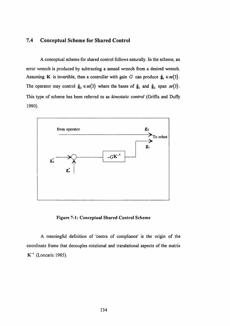
7.4 Conceptual Scheme for Shared Control
A conceptual scheme for shared control follows naturally. In the scheme, an
error wrench is produced by subtracting a sensed wrench from a desired wrench.
Assuming K is invertible, then a controller with gain G can produce g, g 5^(3).
The operator may control gj Gse(3) where the bases o f g, and g^ span 5^(3).
This type o f scheme has been referred to as kinestatic control (Griffis and Duffy
1990).
from operator
g.
g2> To robot
gi
- G K - ‘/
F igure 7-1: C onceptual Shared C ontrol Schem e
A meaningful definition o f 'centre o f compliance' is the origin o f the
coordinate frame that decouples rotational and translational aspects o f the matrix
K (Loncaric 1985).
134
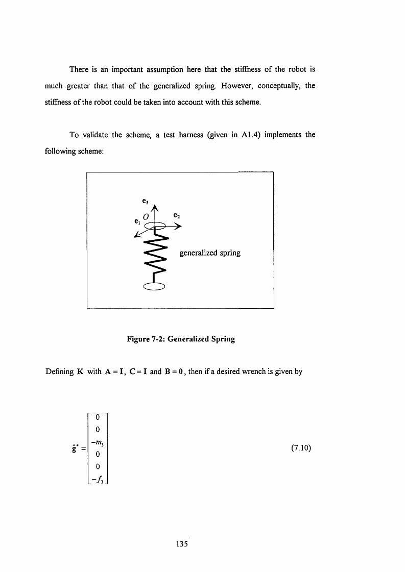
There is an important assumption here that the stiffness o f the robot is
much greater than that o f the generalized spring. However, conceptually, the
stiffness o f the robot could be taken into account with this scheme.
To validate the scheme, a test harness (given in A1.4) implements the
following scheme:
generalized spring
F igure 7-2: G eneralized Spring
Defining K with A = I , C = I and B = 0 , then if a desired wrench is given by
g =
00
-W300
(7.10)
135
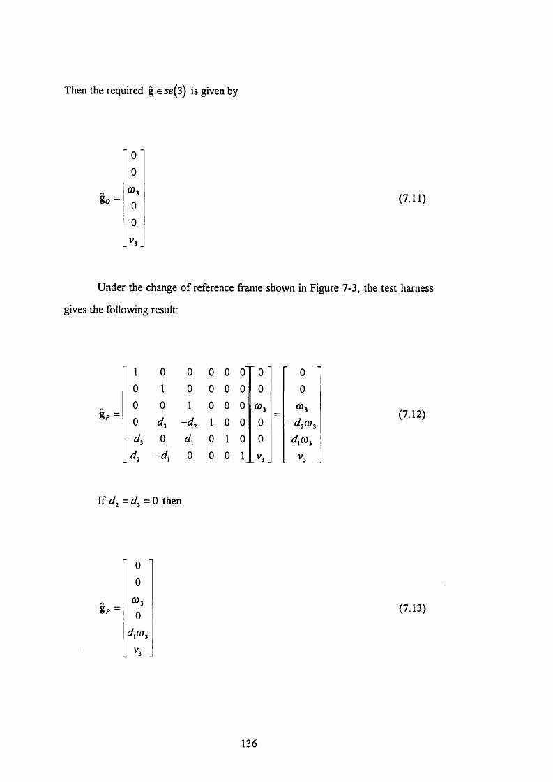
Then the required g € 5^(3) is given by
go =
00
CÜ3
00
V ,
(7.11)
Under the change o f reference frame shown in Figure 7-3, the test harness
gives the following result:
■ 1 0 0 0 0 o' ■ 0 ■ 00 1 0 0 0 0 0 00 0 1 0 0 0 (Ü3 6)3
gp = 0 d. 1 0 0 0 -d^co^
- d . 0 0 1 0 0 d,Cû,
. d . -d , 0 0 0 1 _^3. . 3 .
(7.12)
gp =
00
©3
0d,cù.
(7.13)
136
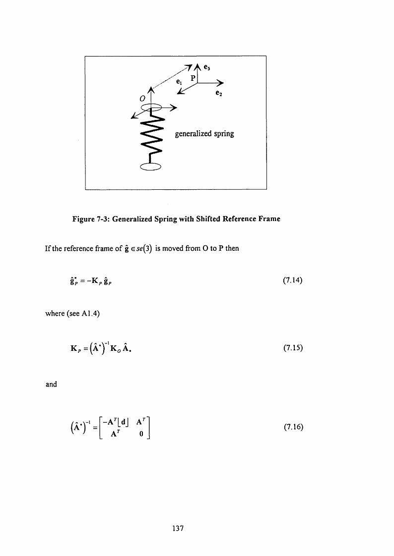
generalized spring
Figure 7-3: G eneralized Spring w ith Shifted Reference F ram e
If the reference frame o f g e jg(3) is moved from O to P then
§ ; = - K p g , (7.14)
where (see A 1.4)
K , = (  ' ) ' ‘K o  . (7.15)
and
- A ’'[dJ A ’' A'' 0
(7.16)
137

The example given above is simple but the theory is applicable to much
more sophisticated compliant devices if they can be characterized by an invertible
stiffness matrix (i.e. where K is symmetric positive definite).
138
Chapter 8
Conclusions
8.1 Overview of the Chapter
In this Chapter, the main contributions o f this thesis are put forward and
discussed. There are many theoretical questions which arise from a proper
geometric discussion o f shared control and teleoperation that have not been
addressed in this thesis; some ideas for future research are presented.
8.2 Contributions of the Thesis
The geometry that underpins shared control (and hybrid position / force
control) is complex and is not generally well understood. The geometric issues
associated with hybrid position / force control have been raised by other authors
using Ball's screw notation (Ball 1900) and results relating to the invariance o f
filter forms have been produced. However, the uptake o f these results has been
slow (Fisher and Mujtaba 1992). In some cases, the results have been openly
challenged (Lawrence and Chapel 1994).
139
In this thesis, the theory o f invariant shared control is presented from a
different perspective using the theory o f differential geometry and Lie groups. The
advantage o f this approach is that the theory is widely used; differential geometry is
the basic tool that physicists use in relativity theory. This is the first presentation o f
an invariant shared control scheme from the perspective o f modem differential
geometry.
It has been shown that the switching matrix is equivalent to a filter which
embodies a Riemannian metric form. Since there is no natural positive definite
metric on SE{2) , the metric needs to be transformed correctly if the measurement
reference frame is moved in order for the filter to work correctly. Alternatively, the
switching matrix can be viewed as a misinterpretation o f a projection operator.
Again, the projection operator needs to be transformed correctly if the
measurement reference frame is moved. This transformation is derived. The
invariance properties o f filter forms are checked using test harnesses.
The role o f compliance in a shared control scheme is analysed. This leads
naturally to a control scheme that has been termed kinestatic control. This is the
first presentation o f the kinestatic control scheme from the perspective o f modem
differential geometry.
8.3 Ideas for Future Research
A major theme in this thesis has been the unification o f ideas under a
consistent theory. There may be scope to continue this unification to cover other
theoretical descriptions that relate to teleoperation. A particularly suitable
candidate may be the theory o f bond graphs. This has been a very successful
140
theoretical tool in the analysis o f energy flows in a bilateral teleoperation system
(Siva 1985).
In the conceptual shared control scheme described in Chapter 6, the
constraint manifold is assumed to be smooth. This greatly simplifies the resulting
analysis. A challenging research objective would be to extend the theoretical
description presented in this thesis to cover the case o f the non-smooth constraint
manifold. One approach may be to view the constraint manifold parametrically and
then to analyse the singularities (Gibson 1995).
The theoretical analysis for the generalized spring given in Chapter 7 could
be extended to cover other physically realizable systems - for example the spring
plus damper. Also the theory has the potential to include the stiffness o f the robot
into the control scheme. This has interesting possibilities for shared control with
flexible robots.
141
References
Altmann, S.L. (1986) Rotations, Quaternions, and Double Groups Oxford :
Clarendon Press
Arnold, V I. (1978) Mathematical Methods of Classical Mechanics New York :
Springer-Verlag
Backes, P.O. (1990) UMI: An Interactive Supervisory and Shared Control System
for Telerobotics Proceedings of IEEE International Conference on Robotics and
Automation
Backes, P.O., Beahan, J., Bon, B. (1993) Interactive Command Building and
Sequencing for Supervised Autonomy Proceedings of IEEE International
Conference on Robotics and Automation
Ball, Sir R.S. (1900) Theorv of Screws Cambridge : Cambridge University Press
Bejczy, A.K. (1980a) Sensors, Controls, and Man-Machine Interface for
Advanced Teleoperation Science, Vol. 208
Bejczy, A.K. (1980b) Kinesthetic Coupling Between Operator and Remote
Manipulator Proceedings of International Conference Tech Conf ASME Centuiw
2 Vol. 1
142
Bejczy, A.K. (1988) Multi-Mode Manual Control in Telerobotics Proceedings of
RoManSv
Bejczy, A.K., Handlykken, M. (1981) Experimental Results with a Six-Degree-
Of-Freedom Force-Reflecting Hand Controller Proceedings of 17th Annual
Conference on Manual Control
Bejczy, A.K., Salisbury, J.K. (1983) Controlling Remote Manipulators Through
Kinesthetic Coupling Computers in Mechanical Engineering
Bicker, R. (1990) Ph.D. Thesis. Department of Mechanical Engineering,
University of Newcastle Upon Tyne
Bottema, O., Roth, B. (1979) Theoretical Kinematics Amsterdam : North-Holland
Publishing Company
Brockett, R.W. (1988) Robotic Manipulators and the Product of Exponentials
Formula Proc. Int. Svmp. Math. Theorv of Networks and Systems
Burdick, J.W. (1989) On the Inverse Kinematics of Redundant Manipulators:
Characterization of the Self-Motion Manifolds Proceedings of IEEE International
Conference on Robotics and Automation
Craig, J.J. (1986) Introduction to Robotics Reading : Addison-Wesley Publishing
Company
Daniel, R.W., Fischer, P.J., Hunter, B. (1993) A High Performance Parallel Input
Device Proceedings of SPIE Telemanipulator Technology and Space Telerobotics
Vol. 2057
Doty, K.L., Melchiorri, C., Bonivento, C. (1993) A Theory of Generalized
Inverses Applied to Robotics The International Journal of Robotics Research.
Vol. 12, N o.l
143
Duffy, J. (1990) Editorial: The Fallacy of Modern Hybrid Control that is Based on
"Orthogonal Complements" of Twist and Wrench Spaces Journal of Robotic
Systems 7(2)
Eppinger, S.D. Steering, W.P. (1987) Understanding Bandwidth Limitations in
Robot Force Control Proceedings of IEEE International Conference on Robotics
and Automation
Featherstone, R. (1987) Robot Dynamics Algorithms Boston : Kluwer Academic
Pubhshers
Fischer, P.J., Daniel, R.W., Siya, K.V. (1990) Specification and Design of Input
Deyices for Teleoperation Proceedings of IEEE International Conference on
Robotics and Automation
Fischer, P J . (1993) Ph.D. Thesis, Department of Engineering Science, Uniyersity
of Oxford
Fisher, W.D., Mujtaba, M.S. (1992) Hybrid Position / Force Control: A Correct
Formulation The International Journal of Robotics Research, V ol.l 1, No.4
Gibson, C.G. (1995) Personal Communication
Gilmore, R. (1974) Lie Groups. Lie Algebras, and Some of Their Applications
New York : John Wiley & Sons
Goertz, R.C., Blomgren, R.A., Grimson, J.H. (1961) The ANL Model 3 Master-
Slaye Electric M anipulator - Its Design and Use in a Caye Proceedings of 9th
Conference on Hot Labs and Equipment
Goertz, R.C. (1964) Manipulator Systems Deyelopment at ANL Proceedings of
12th Conference on Remote Systems Technology
144
Goertz, R.C., Grimson, J., Potts, C. (1966) ANL Mark E4A Electric Master Slave
M anipulator Proceedings of 14th Conference on Remote Systems Technology
Goldstein, H. (1964) Classical Mechanics Reading : Addison-W esley Publishing
Company Inc.
Greenwood, D.T. (1988) Principles of Dynamics New Jersey : Prentice-Hall
International Inc.
Griffis, M., Duffy, J. (1990) Kinestatic Control: A Novel Theory for
Simultaneously Regulating Force and Displacement 21st ASME Mechanisms
Conference
Handlykken, M., Turner, T. (1980) Control System Analysis and Synthesis for a
Six Degree-of-Freedom Universal Force-Reflecting Hand Controller Proceedings
of 19th IEEE Conference on Decision and Control
Hannaford, B. (1989) Stability and Performance Tradeoffs in Bilateral
Telemanipulation Proceedings of IEEE International Conference on Robotics and
Automation
Hayati, S., Venkataraman, S.T. (1989) Design and Implementation of a Robot
Control System with Traded and Shared Control Capability Proceedings of IEEE
International Conference on Robotics and Automation
Hirzinger, G., Heindl, J., Landzettel, K., Brunner, B. (1992) Multisensory shared
autonomy - a key issue in the space robot technology experiment ROTEX
Proceedings of the IEEE / RSJ Conference on Intelligent Robots and Systems
Hirzinger, G., Brunner, B., Dietrich, J., Heindl, J. (1993) Sensor-Based Robotics -
ROTEX and Its Telerobotic Features IEEE Transactions on Robotics and
Automation Vol.9, No.5
145
Hunt, K.H. (1978) Kinematic Geometry of Mechanisms Oxford : Clarendon Press
Kim, W.S. (1990) A Stability Analysis of Shared Compliant Control Japan-USA
Symposium on Flexible Automation
Kim, W.S. (1991) A New Scheme of Force Reflecting Control 5th Annual
W orkshop on Space Operations. Applications and Research (SOAR 9 1 ). NASA
Conference Publication 3127, Vol. 1
Kim, W.S., Hannaford, B., Bejczy, A.K. (1992) Force Reflection and Shared
Compliant Control in Operating Telemanipulators with Time Delay IEEE
Transactions on Robotics and Automation. Vol. 8, No. 2
Lawrence, D.A., Chapel, J.D. (1994) Quantitative Control of M anipulator / Task
Interaction IEEE Control Systems
Loncaric, J. (1985) Geometrical Analysis of Compliant Mechanisms in Robotics
Ph.D. Thesis. Harvard University
Lipkin, H. (1985) Geometry and Mapping of Screws with Applications to the
Hybrid Control of Robotic Manipulators Ph.D. Thesis. University of Florida
Lipkin, H., Duffy, J. (1988) Hybrid Twist and W rench Control for a Robotic
Manipulator Transactions of the ASME Vol. 110
Mason, M. (1981) Compliance and Force Control for Computer Controlled
Manipulators IEEE Trans. Systems, Man and Cybernetics
McAffee, D., Snow, E., Townsend, W. (1990) A New Six-Degree-of-Freedom
Force Reflecting Hand Controller for Space Telerobotics Proceedings of 24th
Aerospace Mechanisms Symposium
146
McAffee, D., Fiorini, P. (1991) Hand Controller Design Requirements and
Performance Issues in Telerobotics 5th International Conference on Advanced
Robotics
McCarthy, J.M. (1990) An Introduction to Theoretical Kinematics Cambridge :
The MIT Press
Mosher, R.S. (1960) An Electrohydraulic Bilateral Servomechanism Proceedings
of 8th Conference on Hot Labs and Equipment
Nakahara, M. (1990) Geometry. Topology and Physics Bristol : Adam Hilger
Normand, J-M (1980) A Lie Group: Rotations in Quantum Mechanics Amsterdam
: North-Holland Publishing Company
Paden, B., S as try, S.S. (1988) Optimal Kinematic Design for a 6R M anipulator
International Journal of Robotics Research. Vol.7
Park, F.C., Pack, D.J. (1991) Motion Control Using the Product of Exponentials
Kinematic Equations Proceedings of IEEE International Conference on Robotics
and Automation
Park, F.C., Brockett, R.W. (1994) Kinematic Dexterity of Robotic Mechanisms
The International Journal of Robotics Research V ol.l3 , N o.l
Park, F.C., Bobrow, I.E. (1995) Efficient Geometric Algorithms for Robot
Kinematic Design Proceedings of IEEE International Conference on Robotics and
Automation
Paul, R.P. (1981) Robot Manipulators: Programming, and Control Cambridge :
The M IT Press
147
Price, J.F. (1977) Lie Groups and Compact Groups Cambridge : Cambridge
University Press
Raibert, M.H., Craig, J J . (1981) Hybrid Position / Force Control of Manipulators
Transactions of ASM E Journal of Dynamic Systems, Measurement and Control,
Vol. 102
Raimondi, T. (1976) Remote Handling in the Joint European Torus (JET) Fusion
Experiment Proceedings of 24th Conference on Remote Systems Technology
Samuel, A.E., McAree, P.R., Hunt, K.H. (1991) Unifying Screw Geometry and
Matrix Transformations The International Journal of Robotics Research. Vol. 10,
No.5
Sattinger, D.H., Weaver, O.L. (1986) Lie Groups and Algebras with Applications
to Physics. Geometry, and Mechanisms New York : Springer-Verlag
Selig, J.M. (1989) Robot Dynamics Using Screw Theory in Robotics: Applied
Mathematics and Computational Aspects Oxford : Oxford University Press
Selig, J.M. (1995) Personal Communication
Siva, K.V. (1985) The Covariant Control System and Its Applications in Remote
and Robotic Manipulations Ph.D. Thesis. University of London
Siva, K.V. (1992) Force Reflecting Telerobotic Systems lEE Lecture
Spivak, M. (1979) A Comprehensive Introduction to Differential Geometry
Berkeley : Publish or Perish Inc
Stein, M.R. (1993) Portability Issues in Teleprogramming: A Case Study
Proceedings of SPIE Telemanipulator Technology and Space Telerobotics
Vol.2057
148
Strang, G. (1986) Introduction to Applied Mathematics W ellesley : Wellesley-
Cambridge Press
Vukobratovic, M., Stojic, R. (1995) Historical Perspective of Hybrid Control in
Robotics: Beginnings, Evolution, Criticism and Trends Mech. Mach. Theorv
Vol.30 No.4
West, H., Asada, H. (1985) A Method for the Design of Hybrid Position / Force
Controllers for Manipulators Constrained by Contact with the Environment
Proceedings of IEEE International Conference on Robotics and Automation
Whitney, D.E, (1969) Resolved Motion Rate Control of Manipulators and Human
Protheses IEEE Transactions on Man-Machine Svstems, Vol. MMS-10, No.2
Wilson, K.B. (1975) Servoarm - A W ater Hydraulic Master-Slave Manipulator
Proceedings of 23rd Conference on Remote Svstems Technoloev
W yboume, B.C. (1974) Classical Groups for Phvsicists New York : John Wiley &
Sons
Yoerger, D R., Slotine, J-J,E. (1987) Supervisory Control Architecture for
Underwater Teleoperation Proceedings of IEEE International Conference on
Robotics and Automation
Yokokohji, Y., Ogawa, A., Hasunuma, H., Yoshikawa, T. (1993) Operating
Modes for Cooperating with Autonomous Functions in Intelligent Teleoperation
Systems Proceedings of IEEE International Conference on Robotics and
Automation
149
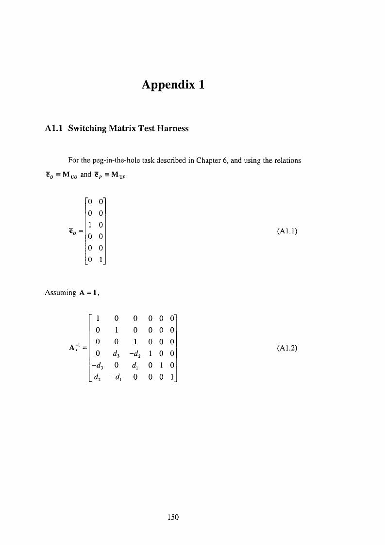
Appendix 1
A 1.1 Switching Matrix Test Harness
For the peg-in-the-hole task described in Chapter 6, and using the relations
0 O'
0 01 0 0 0 0 0 0 1
(A l.l)
Assuming A = I ,
a :-1
1 0 0 0 0 o'0 1 0 0 0 00 0 1 0 0 00 3 -d i 1 0 0
“ 3 0 d. 0 1 0
.^2 -d, 0 0 0 1
(A1.2)
150
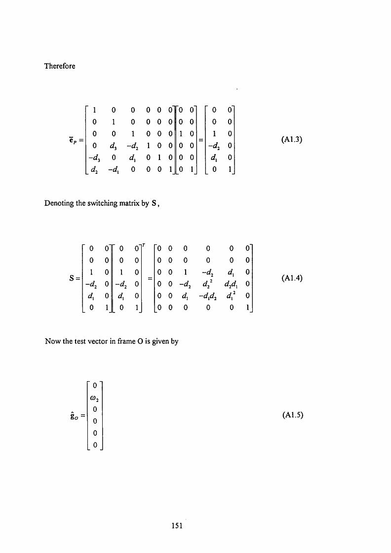
Therefore
Cp —
■ 1 0 0 0 0 o' "0 o' ■ 0 o'0 1 0 0 0 0 0 0 0 00 0 1 0 0 0 1 0 1 00 - 4 1 0 0 0 0 -^2 0
- 4 0 0 1 0 0 0 d, 00 0 0 1 0 1 0 1
(A1.3)
Denoting the switching matrix by S ,
S =
' 0 o' ■ 0 o' T "0 0 0 0 0 O'
0 0 0 0 0 0 0 0 0 01 0 1 0 0 0 1 -d . d. 0
-d^ 0 -d . 0 0 0 d d A 0
d, 0 d, 0 0 0 d, - d A d" 00 1 _ 0 1 0 0 0 0 0 1
(A1.4)
N ow the test vector in frame O is given by
ëo =
0Û),
0000
(A l.5)
151
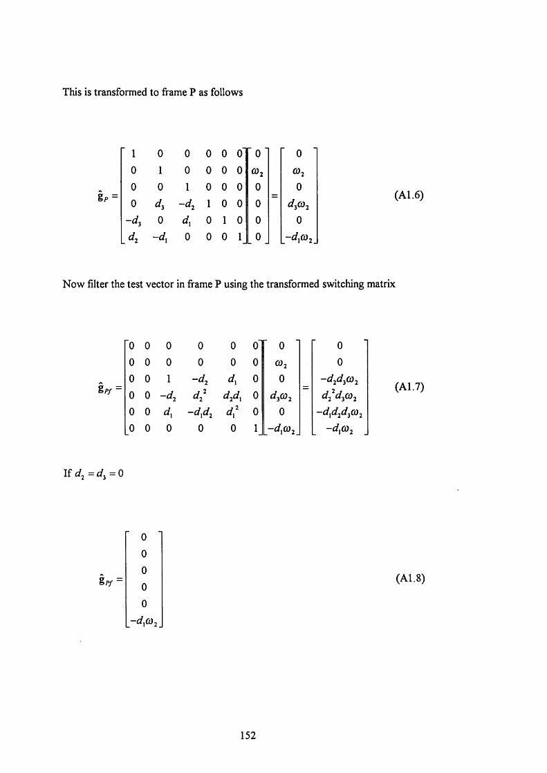
This is transformed to frame P as follows
gp =
■ 1 0 0 0 0 o' ' 0 ' 00 1 0 0 0 0 ©2 ©20 0 1 0 0 0 0 00 3 -^2 1 0 0 0 i/3©2
-^3 0 0 1 0 0 00 0 0 1 0 -d,œ,_
(A1.6)
N ow filter the test vector in frame P using the transformed switching matrix
"0 0 0 0 0 o' 0 00 0 0 0 0 0 ©2 00 0 1 d 0 0 -d d (Ù2
èpf - 0 0 d^d, 0 i/3©2 d^d-fi)^0 0 d, ~d\dj d. 0 0 -dxdjd Cù0 0 0 0 0 1 _-i/,©2_ _ -d G _
(A1.7)
%pf -
00000
-d^CÛ2
(A1.8)
152
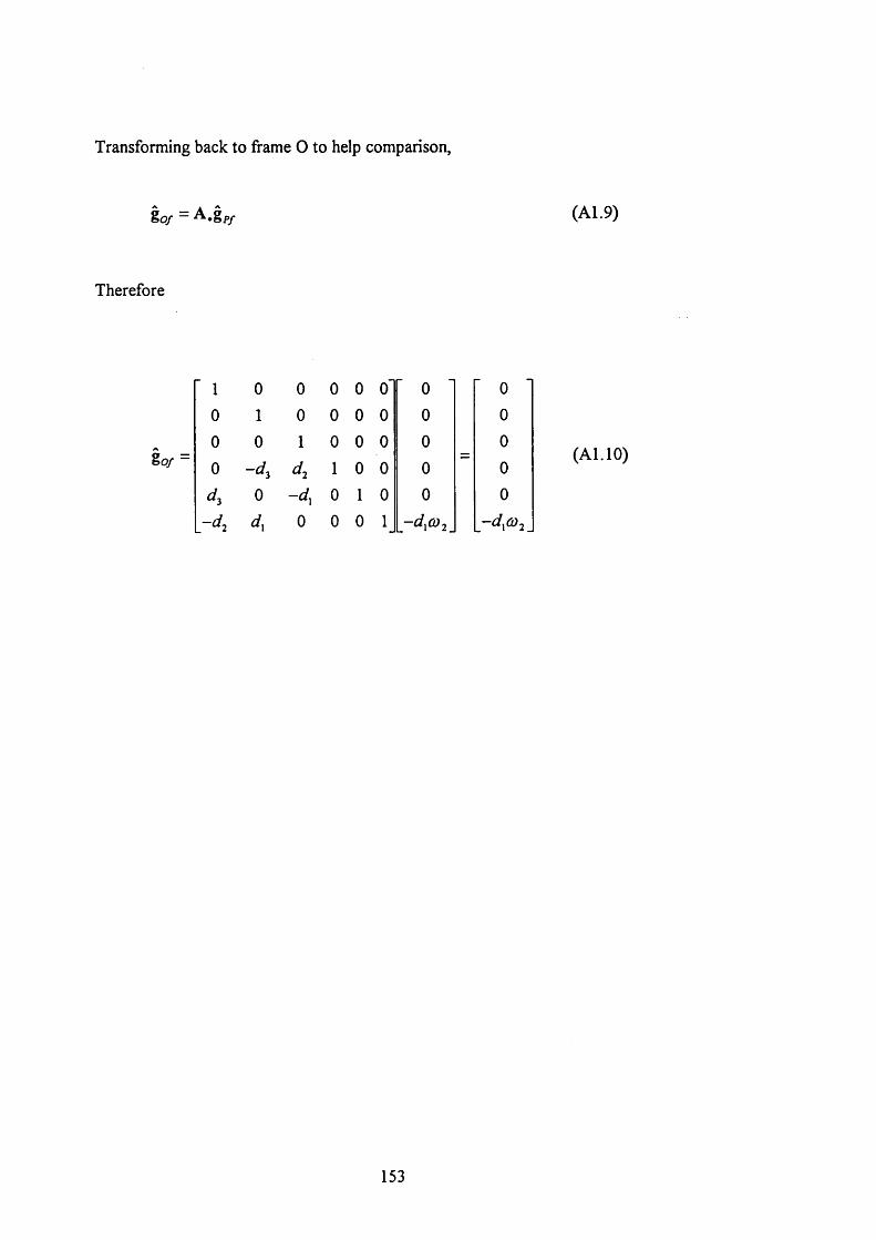
Transforming back to frame O to help comparison,
go/ = A . g p / (A1.9)
Therefore
So/ =
1 0 0 0 0 o' 0 00 1 0 0 0 0 0 00 0 1 0 0 0 0 00 -^3 1 0 0 0 0
0 -d, 0 1 0 0 00 0 0 1 rd \^ 2 . .~d\^2_
( A l . l O )
153
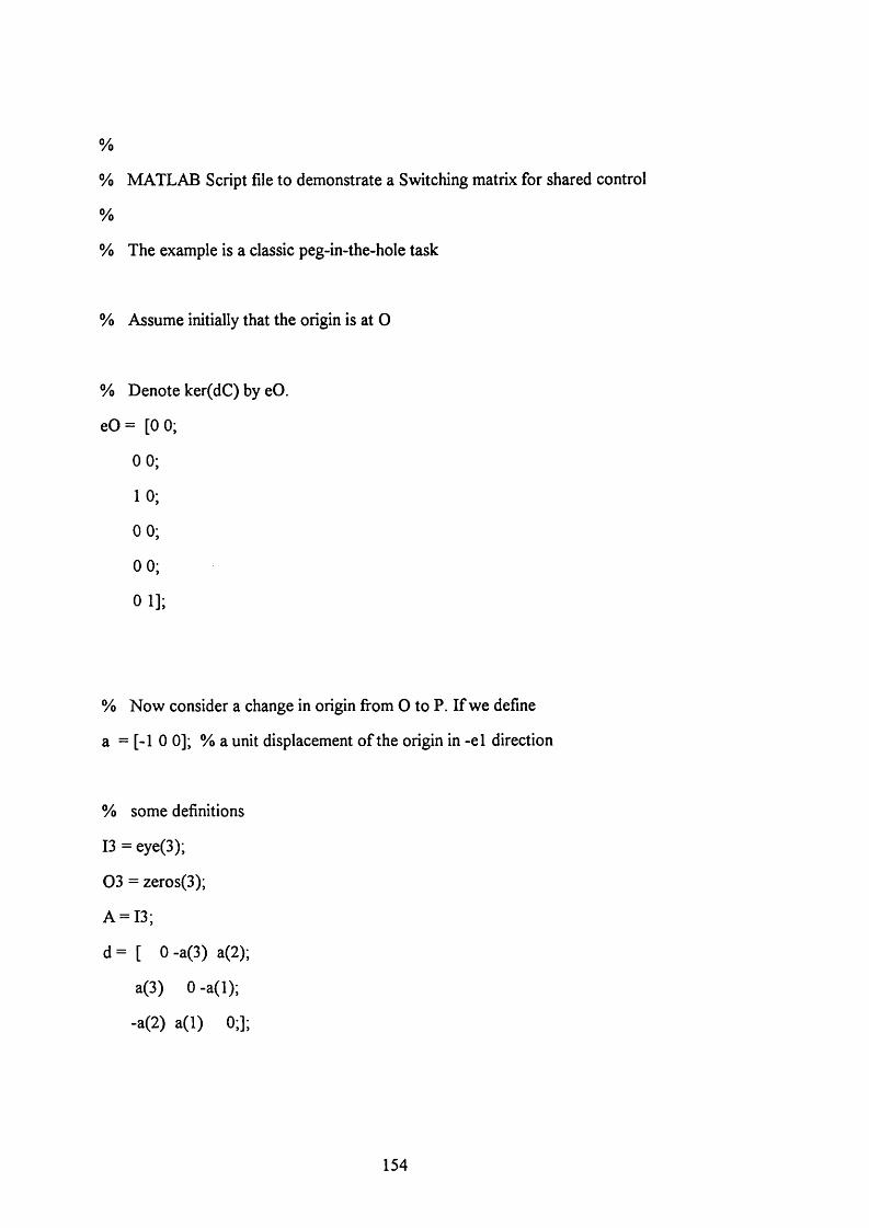
%
% MATLAB Script file to demonstrate a Switching matrix for shared control
%
% The example is a classic peg-in-the-hole task
% Assume initially that the origin is at O
% Denote ker(dC) by eO.
eO = [0 0;
0 0;
10;
0 0;
0 0;
0 1];
% Now consider a change in origin from O to P. If we define
a = [-1 0 0 ]; % a unit displacement of the origin in -el direction
% some definitions
13 = eye(3);
03 = zeros(3);
A = 13;
d = [ 0-a(3)a(2);
a(3) O-a(l);
-a(2) a(l) 0;];
154
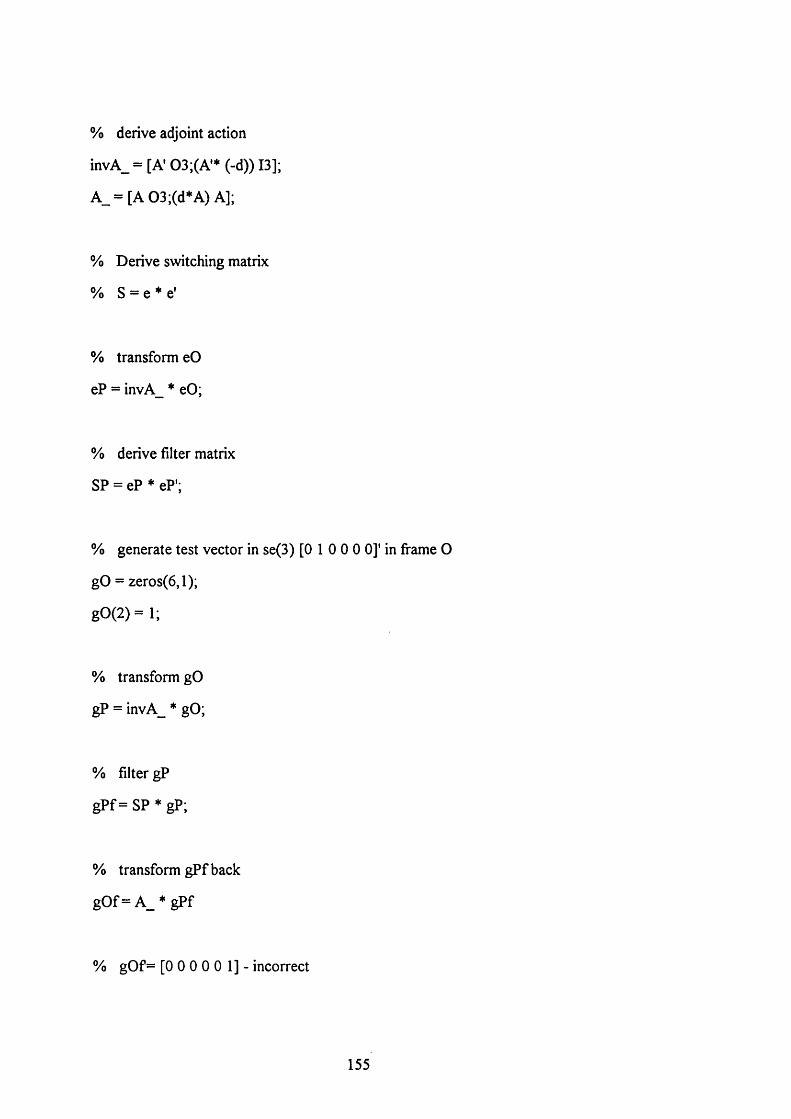
% derive adjoint action
in v A _ = [A '0 3 ;(A '* (-d)) 13];
A_ = [A 03;(d*A ) A];
% Derive switching matrix
% S = e * e'
% transform eO
eP = invA_ * eO;
% derive filter matrix
SP = eP * eP';
% generate test vector in se(3) [0 1 0 0 0 0 ] ' in frame O
gO = zeros(6,l);
g O ( 2 ) = l ;
% transform gO
gP = invA_ * gO;
% filter gP
gP f = SP * gP;
% transform gP f back
gO f = A_ * gPf
% gO f= [ 0 0 0 0 0 1] - incorrect
155
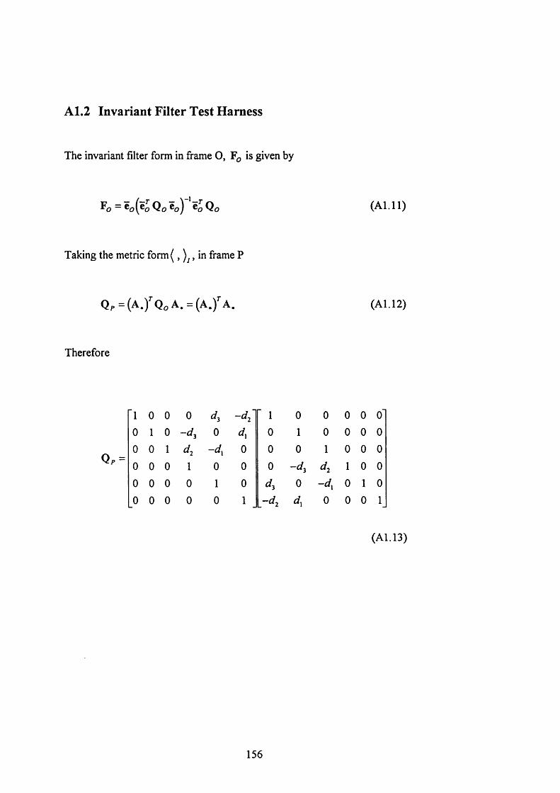
A1.2 Invariant Filter Test Harness
The invariant filter form in frame O, is given by
F o = ë o ( ê j Q o ë o ) ‘ ' ê j Q o (A l ,11)
Taking the metric fo rm ( , , in frame P
Q p = (a . ) " Q o A . = (a . / a . (A1.12)
Therefore
Q p =
"1 0 0 0 3 1 0 0 0 0 o'0 1 0 -^3 0 0 1 0 0 0 00 0 1 4 0 0 0 1 0 0 00 0 0 1 0 0 0 -^3 d2 1 0 00 0 0 0 1 0 3 0 -d . 0 1 00 0 0 0 0 1 .-^2 d, 0 0 0 1
(A1.13)
156
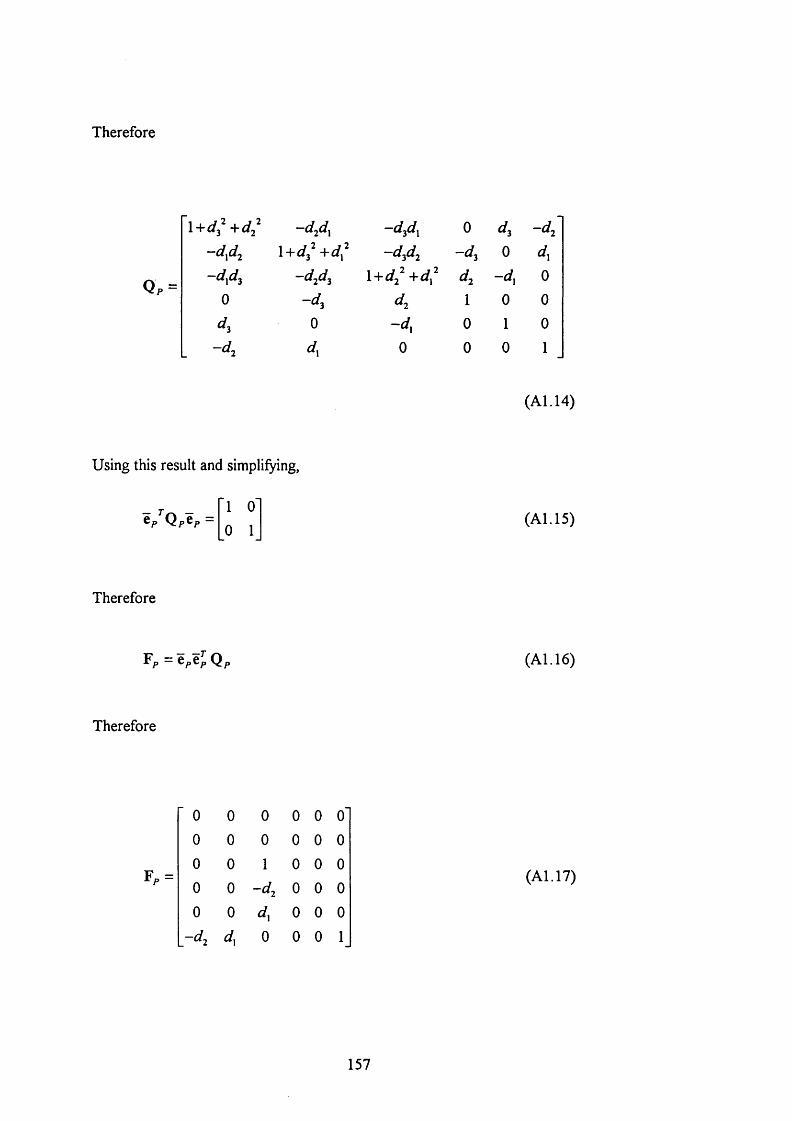
Therefore
Qp -
1+ + dj -d d -djd^ 0 d. -d^l+d,^+d,^ -d,d^ - 4 0 d.
-d d l+dj ~ d d -d. 00 - 4 4 1 0 0
0 -d. 0 1 0
-^2 d, 0 0 0 1
Using this result and simplifying,
(A1.14)
tp^QpCp =1 0 0 1
(A1.15)
Therefore
Fp = ep€pQ p (A1.16)
Therefore
Pp =
0 0 0 0 0 00 0 0 0 0 00 0 1 0 0 00 0 -d^ 0 0 00 0 d. 0 0 0
-d^ d, 0 0 0 1
(A1.17)
157
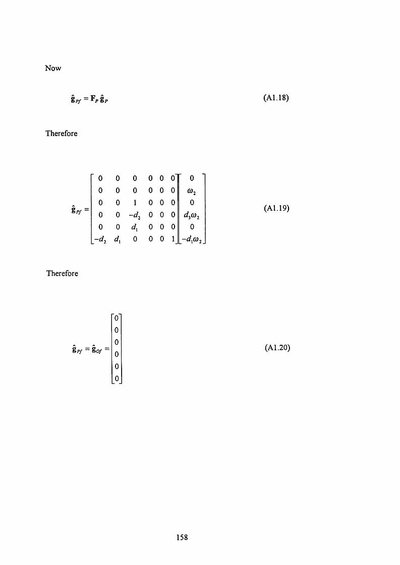
N ow
(A l. 18)
Therefore
gp/ -
■ 0 0 0 0 0 G' 0
0 0 0 0 0 0 Û>20 0 1 0 0 0 0
0 0 -d^ 0 0 0 d^(ù^
0 0 d, 0 0 0 0
- 4 d, 0 0 0 1 .~ d \^ 2 .
(A l. 19)
Therefore
gp/ = go/ = (A l.20)
158

%
% MATLAB Script file to demonstrate an Invariant filter for shared control
%
% The example is a classic peg-in-the-hole task
% Assume initially that the origin is at O
% Denote ker(dC) by eO.
eO = [0 0;
0 0;
10;
0 0;
0 0;
0 1];
% N ow consider a change in origin from O to P. I f we define
a = [ 1 0 0]; % a unit displacement o f the origin in -e l direction
% some definitions
13 = eye(3);
0 3 = zeros(3);
A = 13;
d = [ 0 -a (3 ) a(2);
a(3) O -a(l);
-a(2) a ( l) 0;];
159
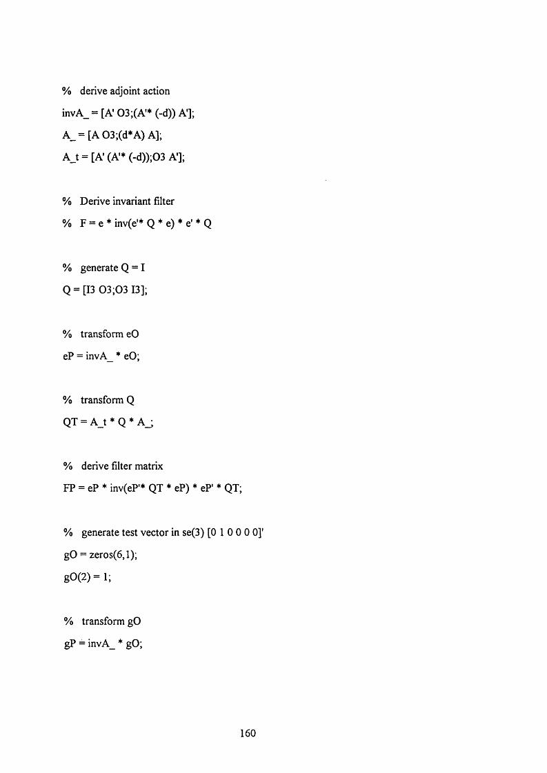
% derive adjoint action
invA _= [A' 0 3 ;(A * (-d)) A'];
A _ = [A 03;(d*A ) A];
A_t = [A (A ’* (-d ));0 3 A’];
% Derive invariant filter
% F = e * inv(e'* Q * e) * e' * Q
% generate Q = I
Q = [I3 0 3 ;0 3 13];
% transform eO
eP = invA_ * eO;
% transform Q
QT = A t * Q * A_j
% derive filter matrix
FP = eP * inv(eP'* QT * eP) * eP' * QT;
% generate test vector in se(3) [0 1 0 0 0 0 ] '
gO = zeros(6,l);
gO(2) = 1;
% transform gO
gP = invA_ * gO;
160
% filter gP
gPf=FP * gP;
% transform gPf back
gOf = A * gPf
% gOf = [0 0 0 0 0 0] as expected
161
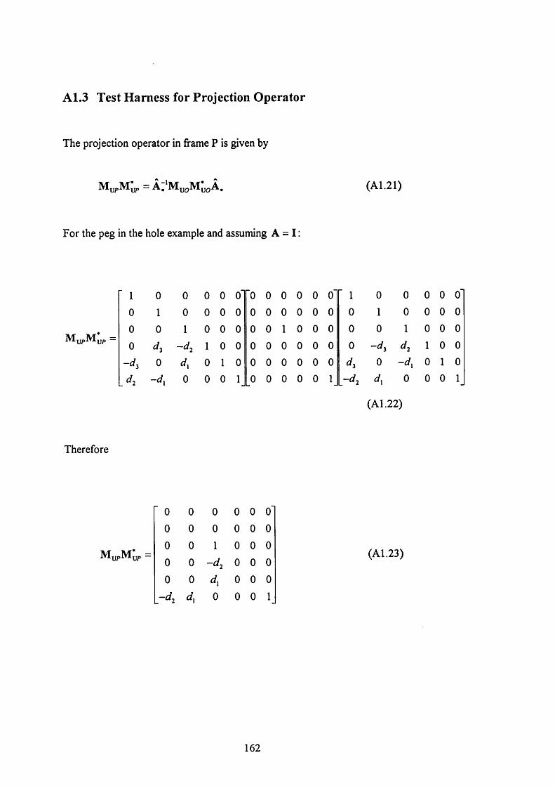
A1.3 Test Harness for Projection Operator
The projection operator in frame P is given by
(A1.21)
For the peg in the hole example and assuming A = I :
Mu/>Mup —
■ 1 0 0 0 0 o' ■Q 0 0 0 0 o' ' 1 0 0 0 0 o'0 1 0 0 0 0 0 0 0 0 0 0 0 1 0 0 0 00 0 1 0 0 0 0 0 1 0 0 0 0 0 1 0 0 00 - 4 1 0 0 0 0 0 0 0 0 0 -^3 4 1 0 0
-d^ 0 d, 0 1 0 0 0 0 0 0 0 d. 0 -d , 0 1 0
J 2 0 0 0 1 0 0 0 0 0 1 - 4 0 0 0 1
Therefore
(A1.22)
MupMup —
0 0 0 0 0 00 0 0 0 0 00 0 1 0 0 00 0 -d 0 0 00 0 d, 0 0 0
- 4 d, 0 0 0 1
(A1.23)
162
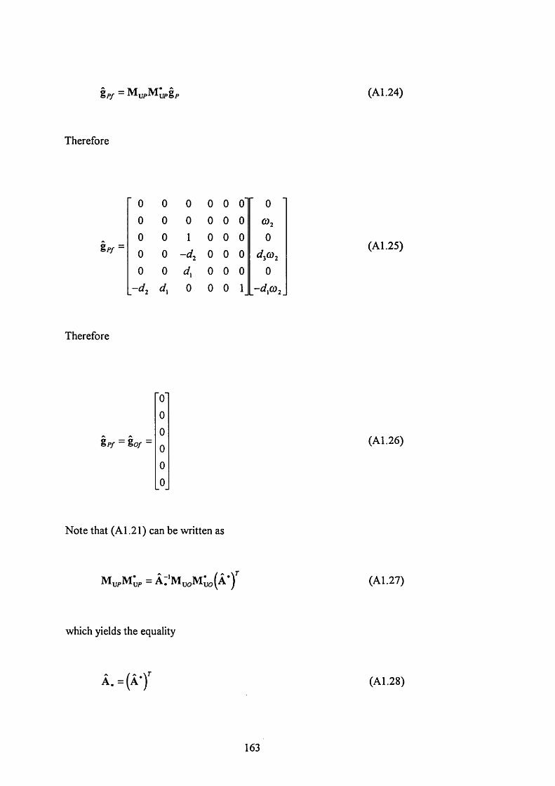
gpy — M ypM upgp (A l.24)
Therefore
S f/ =
■ 0 0 0 0 0 o' 0
0 0 0 0 0 0
0 0 1 0 0 0 0
0 0 -d . 0 0 0 d coj0 0 d, 0 0 0 0
.-^2 0 0 0 1 .-dxCÙ2_
(A1.25)
Therefore
8 p/ - go/ - (A1.26)
N ote that (A1.21) can be written as
(A l .27)
which yields the equality
A .= (Â -) ’' (A1.28)
163
%
% MATLAB Script file to demonstrate a Projection operator for shared control
%
% The example is a classic peg-in-the-hole task
% Assume initially that the origin is at O
% Denote ker(dC) by eO.
e O = [0 0;
0 0;
10 ;
0 0;
0 0;
0 1];
estarO = [0 0;
0 0;
10 ;
0 0;
0 0;
0 1];
% N ow consider a change in origin from O to P. I f we define
a = [ - 1 0 0 ] ; % a unit displacement o f the origin in -e l direction
164
% some definitions
13 = eye(3);
0 3 = zeros(3);
A = 13;
d = [ 0 -a (3 ) a(2);
a(3) O -a(l);
-a(2) a ( l) 0;];
% derive adjoint action for se(3)
in v A _ = [A '0 3 ;(A '* (-d ))I3 ];
A _ = [A 03;(d*A ) A];
% derive adjoint action for se*(3)
in v A 2 _ = [A (A * (-d));03 13];
A 2 _ = [A (d*A );03 A];
invA2_t = [A 03;(d*A ) A];
% Derive projection matrix
% PM = M * M star
M O = eO;
M starO=estarO';
PM O = MO * MstarO;
% generate test vector in se(3) [0 1 0 0 0 0 ] ' in frame O
gO = zeros(6,l);
g O ( 2 ) = l ;
165
% filter gO
gO f = PM O * gO; % [0 0 0 0 0 0] as expected
% derive transformed projection matrix
% transform PMO
PM P = invA_ * PM O * A j
% transform gO
gP = invA_ * gO;
% filter gP
gP f = PM P * gP;
% transform gP f back
gO f = A_ * gPf; % [0 0 0 0 0 0] as expected
% derive transformed projection matrix another way
% transform MO and MstarO
MP = invA_ * MO;
M starP = M starO * invA2_t;
% Derive projection matrix
% PM = M * M star
PM P = MP * MstarP;
166
% filter gP
gP f = PM P * gP;
% transform g P f back
gO f = A_ * gPf; % [0 0 0 0 0 0] as expected
167
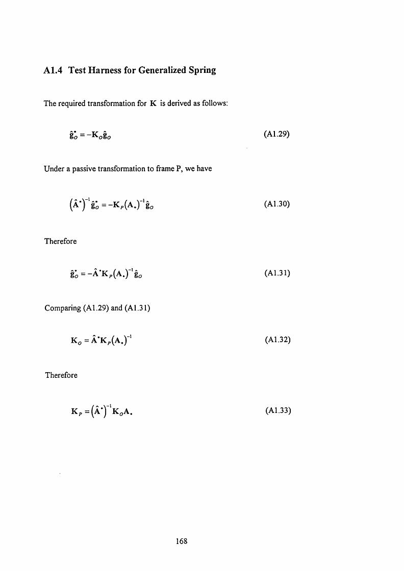
A1.4 Test Harness for Generalized Spring
The required transformation for K is derived as follows:
èo = - ^ o è o (A I.29)
U nder a passive transformation to frame P, we have
( Â - ) '‘g ô = - K , ( A . ) ' 'g o (A l.30)
Therefore
g ô = - Â - K ^ ( A .) - 'g „ (A l .31)
Comparing (A 1.29) and (A 1.31)
K o = Â 'K ^ ( A ,) ' ' (A l .32)
Therefore
K p = ( Â ') " K o A . (A l .33)
168
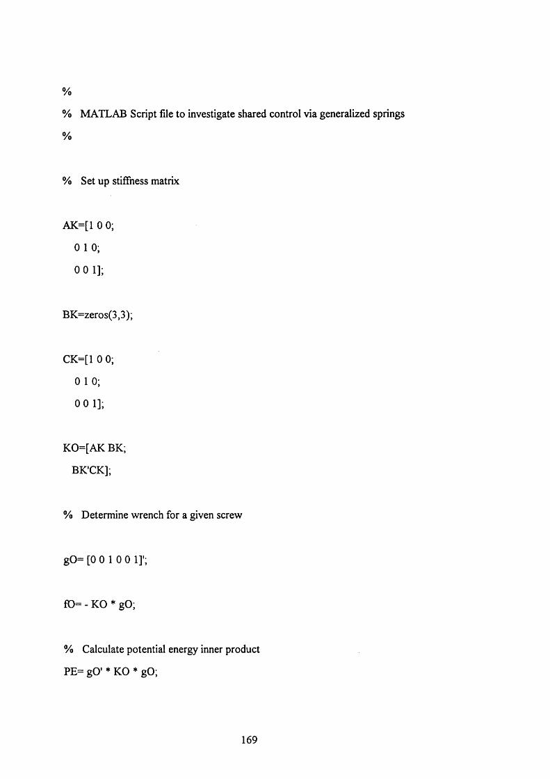
%
% MATLAB Script file to investigate shared control via generalized springs
%
% Set up stiffness matrix
AK=[1 0 0;
0 1 0;
0 0 1];
BK=zeros(3,3);
CK=[1 0 0;
0 1 0;
0 0 1];
KO=[AK BK;
BK'CK];
% Determine wrench for a given screw
gO= [0 0 1 0 0 1]';
fO= - KO * gO;
% Calculate potential energy inner product
PE= gO ’ * KO * gO;
169
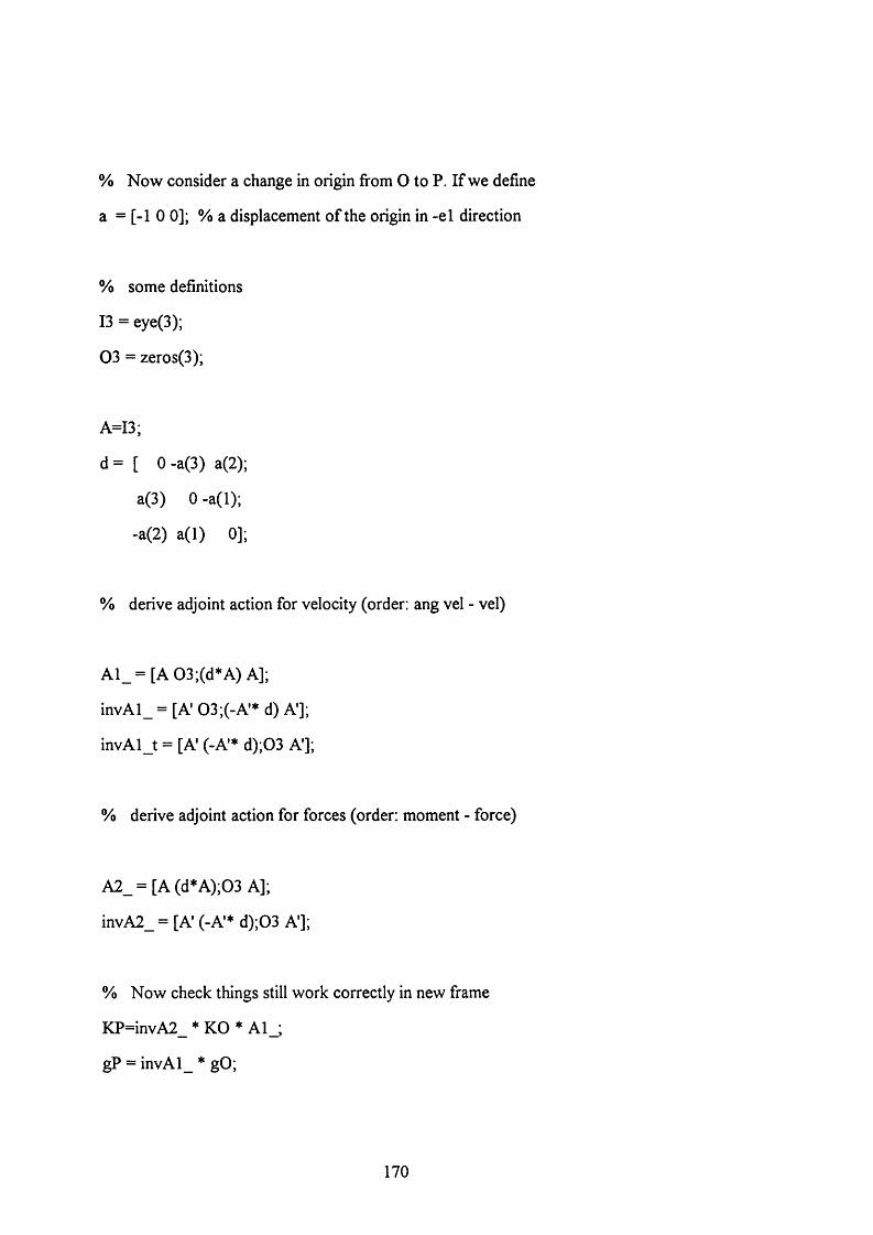
% N ow consider a change in origin from O to P. I f we define
a = [ - 1 0 0 ] ; % a displacement o f the origin in -e l direction
% some definitions
13 = eye(3);
0 3 = zeros(3);
A=I3;
d = [ 0 -a (3 ) a(2);
a(3) 0 -a (l);
-a(2) a ( l) 0];
% derive adjoint action for velocity (order: ang vel - vel)
A 1 _ = [A 03;(d*A ) A];
invA l_ = [A 03 ;(-A * d) A'];
in v A lJ = [A (-A * d);03 A ];
% derive adjoint action for forces (order: moment - force)
A 2 _ = [A (d*A );03 A];
in v A 2 _ = [A (-A * d);03 A ];
% N ow check things still work correctly in new frame
KP=invA2_ * KO * A l_ ;
gP = invA l_ * gO;
170
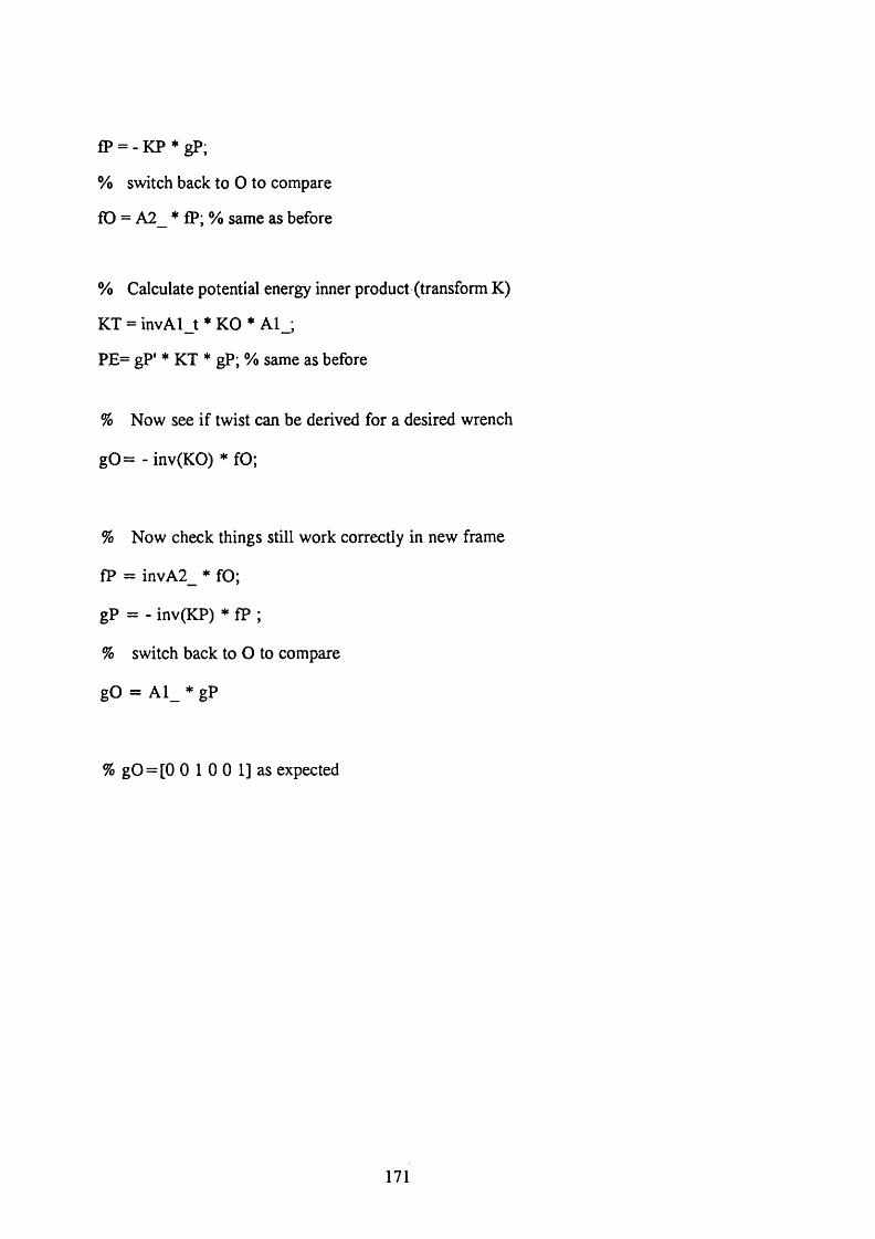
fp = - KP * gP;
% switch back to 0 to compare
fO = A 2_ * fp; % same as before
% Calculate potential energy inner product (transform K)
KT = in v A lJ * KO * A l j
PE= gP' * KT * gP; % same as before
% Now see if twist can be derived for a desired wrench
g O = - inv(KO) * fO;
% Now check things still work correctly in new frame
fP = invA2_ * fO;
gP = - inv(KP) * fP ;
% switch back to O to compare
gO = A l_ * gP
% gO = [0 0 1 0 0 1] as expected
171
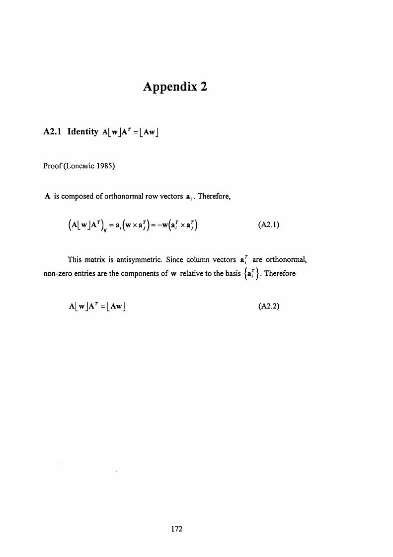
Appendix 2
A2.1 Identity A [w JA ^ = [A w J
P roo f (Loncaric 1985):
A is composed o f orthonormal row vectors a , . Therefore,
(a [ w JA^)^^ = a,.(w x a j ) = - w ( a f x a j ) (A2.1)
This matrix is antisymmetric. Since column vectors a f are orthonormal,
non-zero entries are the components o f w relative to the basis | a f J . Therefore
A [ w J A ^ = L A w J (A2.2)
172
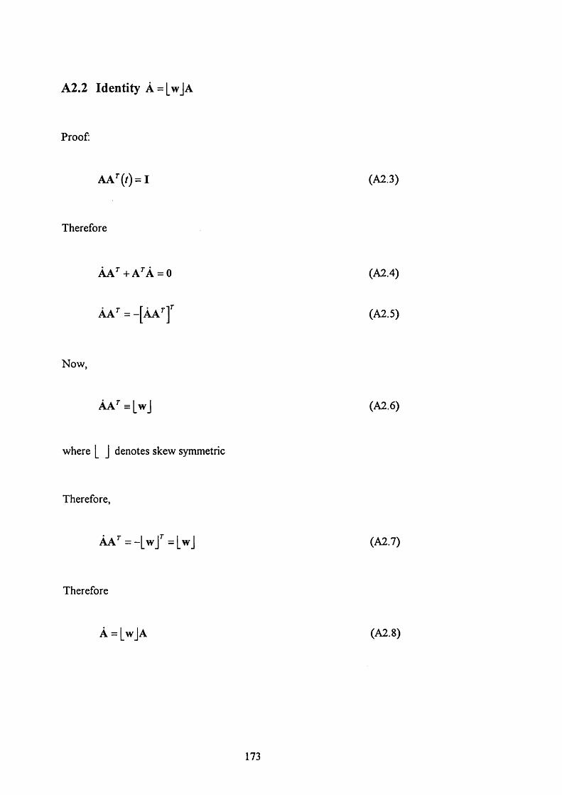
A2.2 Identity À = [w jA
Proof:
A A ''(r) = I (A2.3)
Therefore
À A ’'+ A ’'À = 0 (A2.4)
À A ’' = (A2.5)
Now,
À A ^ = [ w J (A2.6)
w here |_ J denotes skew symmetric
Therefore,
ÀA^ = - [ w j^ = [w j (A2.7)
Therefore
À = [ wJA (A2.8)
173
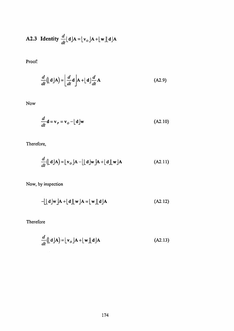
A2.3 Identity ^[djA = [vqJa +[wj[djA
Proof:
| ( L ‘ * J A ) = dt ( « » )
N ow
dtd = Vp = Vq - |_ d jw (A2.10)
Therefore,
— ([d jA ) = [ v o jA - [ [ d J w jA + [dJLw jA (A2.11)
Now, by inspection
- [ [ d J w jA + [d J [w jA = |_wJ|_djA (A2.12)
Therefore
— ([d jA ) = [ v ^ j A + [w J[d jA (A2.13)
174
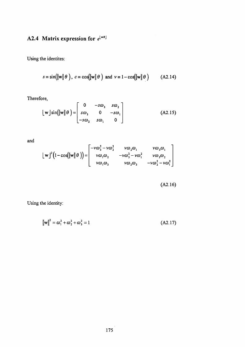
A2.4 Matrix expression for
Using the identités:
s = sin(||w|| 0 ) , c = cos(||w|| 0 ) and v = 1 - cos(||w|| 6 ) (A 2.14)
Therefore,
[ w js in ( ||w |e )
G —5CD3 SCÙ2
SCÙ^ G —SCÛ^ (A2.15)
- S C Û 2 G
and
[ w /( l - c o s ( | |w | |0 ) ) =
-vcûl-vcûl
va),û)2
V Û ) ,Û ) 3
Vfüjû),
- V Û ) 3 - V û ) f
vcû^cûj
VCû Cù
VÛ) Û)2
- V C û l - V û ) f
Using the identity:
(A2.16)
\w f +cùl+cû] = \ (A2.17)
175
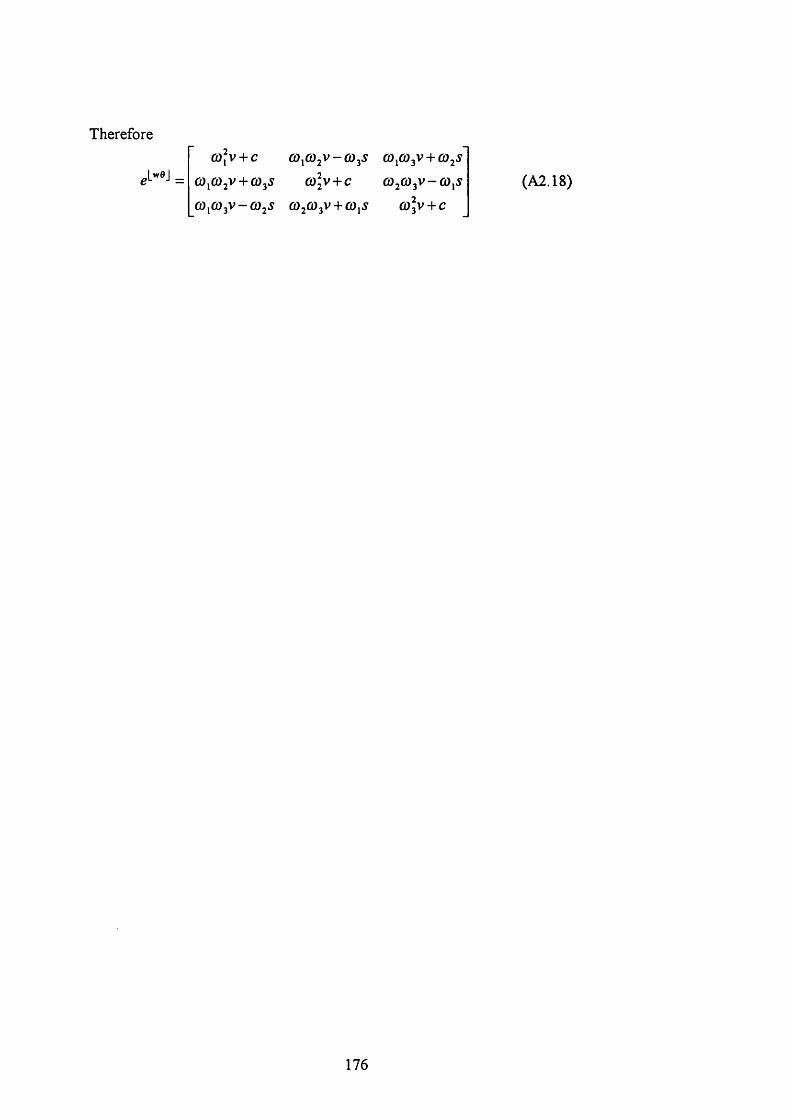
Therefore
,L"*J _û),v + c
(Ù (Û V-\-CÙ S
cù cû v-œ s cû û)jV + cù2Sœ iv + c
CÙ^CÛ^V-œ2S CÛ2(Û2V + CÛ S
Û)2Û)3V-Û),5
(Ü 3 V + C
(A2.18)
176
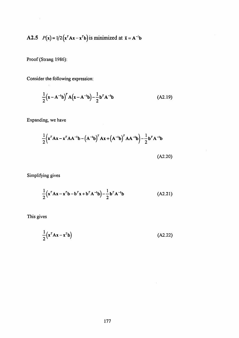
A2.5 P (x ) = 1/2 Ax - x^b) is minimized at x = A "’b
P ro o f (Strang 1986):
Consider the following expression:
i ( x - a (i - A ' b ) - b ’'A ‘'b (A 2.19)
Expanding, we have
^ |x ^ Ax - X AA b - (A '^b)^ Ax + (A ”*b)^ AA"*bj - b^ A ‘*b
(A2.20)
Simplifying gives
■i^x^Ax - x^b - b^x + b^A"‘b ) - ^ b ^ A 'b (A2.21)
This gives
—( x ^ A x- x ^ b ) (A2.22)
177

So the minimum o f (A2.22) is at
X = A 'b (A2.23)
which brings the first term in (A2.19) to zero.
178