Annali di MatematicaDOI 10.1007/s10231-012-0259-9

Shape derivatives in differential forms I: an intrinsicperspective

Ralf Hiptmair · Jingzhi Li

Received: 7 July 2011 / Accepted: 4 February 2012© Fondazione Annali di Matematica Pura ed Applicata and Springer-Verlag 2012

Abstract We treat Zolésio’s velocity method of shape calculus using the formalism ofdifferential forms, in particular, the notion of Lie derivative. This provides a unified andelegant approach to computing even higher-order shape derivatives of domain and boundaryintegrals and avoids the tedious manipulations entailed by classical vector calculus. Hithertounknown expressions for shape Hessians can be derived with little effort. The perspective ofdifferential forms perfectly fits second-order boundary value problems (BVPs). We illustrateits power by deriving the shape derivatives of solutions to second-order elliptic BVPs withDirichlet, Neumann and Robin boundary conditions. A new dual mixed variational approachis employed in the case of Dirichlet boundary conditions.

Keywords Differential forms · Lie derivative · shape derivative ·Hadamard structure theorems · dual formulation

Mathematics Subject Classification (2000) 35B37 · 49J20 · 58A10

1 Introduction

Shape calculus, which is the differentiation of functionals and operators with respect tovariations of a spatial domain, is one of the mathematical foundations of shape sensitivityanalysis and shape optimization. Here, the control variable is no longer a set of parameters orfunctions but the shape or structure of a geometric object. For a comprehensive presentation,the reader is referred to the monograph [6]. In this work, shape calculus is approached via

R. HiptmairSAM, ETH Zurich, 8092 Zurich, Switzerlande-mail: hiptmair@sam.math.ethz.ch

J. Li (B)South University of Science and Technology of China, Shenzhen 518055, People’s Republic of Chinae-mail: jzlicuhk@gmail.com

123

R. Hiptmair, J. Li

the velocity method, that is, shape perturbations are governed by flows generated by spatialvector fields. This paradigm of shape calculus will be adopted throughout the paper.

In this article, we derive shape derivatives using the calculus of differential forms asopposed to classical vector calculus. One might object that no new insights can be expected,because vector analysis offers a model “isomorphic” to the calculus of differential forms.Nevertheless, in our opinion, adopting differential forms brings a significant reward, for thefollowing reasons:

– Differential forms facilitate the unified treatment of different spatial dimensions anddifferent classes of boundary value problems (BVPs) and functionals corresponding todifferent orders of forms.

– The velocity method of shape calculus neatly fits the concept of Lie derivative, which isnatural for differential forms.

– The calculus of differential forms can often use simple formulas, where vector calculushas to resort to complicated expressions.

– Differential forms offer a coordinate independent description of models, whereas vectorcalculus will depend on coordinates, whose choice is often arbitrary.

– Differential forms clearly separate terms that are invariant with respect to homeomorphictransformations and those that depend on metric.

– The exterior derivative of differential forms is the natural language for expressing conser-vation principles underlying many PDE-based models. It is the key differential operatoroccurring in second-order BVPs. Shape derivatives of their solutions play a central rolein shape optimization.

The aim of this first paper is twofold. Firstly, we use the exterior calculus of differentialforms and the Lie derivative to rederive the renowned Hadamard structure theorem [9], whichessentially states that shape derivatives depend only on the normal component of the defor-mations on the boundary of the reference domain. We demonstrate how higher-order shapederivatives can be derived recursively by repeating the argument in the proof of first-ordershape gradients.

Secondly, in the case of a second-order PDE with various boundary conditions, we illus-trate how to determine the concrete shape derivatives of solutions of variational problems byapplying our abstract structure theorems. In particular, we find that via a dual formulation, theboundary condition for the shape derivative of the solution of an elliptic PDE with Dirichletboundary condition can be obtained rigorously in the weak sense. This is one of the severalnew results presented in this article.

The outline of the paper is as follows: Sect. 2 presents important notations and definitionsconnected with differential forms. Section 3 is devoted to the proof of structure theoremsof shape derivatives by the exterior calculus of differential forms. In particular, the shapeHessians of domain and boundary integrals are further investigated, with emphasis on theasymmetry due to the Lie bracket of two velocity fields associated with the transformations.In Sect. 4, we reinterpret the abstract theory in Sect. 3 in terms of vector proxies, namely scalarfunctions and vector fields, with emphasis on the shape gradient and Hessian of domain andboundary integrals, bilinear forms, and normal derivatives. In Sect. 5, by a model problem,we illustrate the machinery for how to express the abstract structure theorems for second-order elliptic BVPs with natural (Neumann and Robin) boundary conditions. In Sect. 6, wederive, in particular via variational methods, the Dirichlet boundary conditions supplement-ing with the PDE for the shape derivative of the solution to the Dirichlet problem in the dualformulation.

123

Shape derivatives in differential forms I

2 Preliminaries

2.1 Notations

The interior and closure of a set A ⊂ Rn will be denoted, respectively, by int A andA. Throughout the paper, the classical Euclidean space Rd (d ∈ N, d ≥ 2) of dimen-sion d is equipped with the canonical orthonormal bases e j ’s, 1 ≤ j ≤ d , and norm

|x| :=√

x21 + · · · + x2

d for x = (x1, . . . , xd)T ∈ Rd , and inner product ⟨x, y⟩. The canonical

orthonormal basis of Rd corresponds to a dual basis of (Rd)∗, i.e., dx1, dx2, . . . , dxd withdxi (e j ) = 1 if i = j and zero otherwise.

2.2 Differential forms

In this subsection, we briefly review some important notions and results about the exterior cal-culus of differential forms. Readers may refer to [4,8] for a detailed exposition of differentialforms.1

A differential form ω of degree l, l ∈ N0 = {0} ∪ N, and class Cm, m ∈ N0, in somedomain ! ⊂ Rd , is a mapping with values in the space of alternating l-multilinear forms

∧l

on Rd :

ω =∑

I

ωI dxI : x ∈ ! ⊂ Rd )→ ω(x) ∈∧l

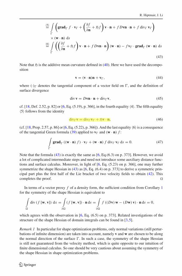
, (1)

where all the componentsωI (x) ∈ Cm(!), and summation is over all the increasing l-permu-tations I = (i1, . . . , il), with 1 ≤ i1 < · · · < il ≤ d , and we denote dxI = dxi1∧ · · · ∧dxil .Hereafter, we write ω ∈ DF l,m(!). In an analogous way, we can define DF l,∞(!) if allωI (x) ∈ C∞(!), and DF l,∞

0 (!) if all ωI (x) ∈ C∞0 (!). Likewise, Hs

(!;∧l(Rd)

)(s ∈

R+0 ) denotes the space consisting of all differential forms with each component in Hs(!),

which can be viewed as the Hilbert space obtained by means of the completion of DF l,∞(!)

with respect to the norm

∥ω∥2Hs

(!;∧l (Rd )

) :=∑

I

∥ωI ∥2Hs (!) . (2)

In particular, we use L2(!;∧l(Rd)) instead of H0(!;∧l(Rd)

).

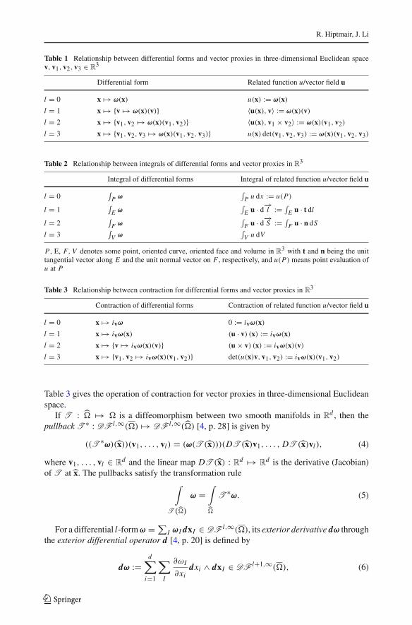
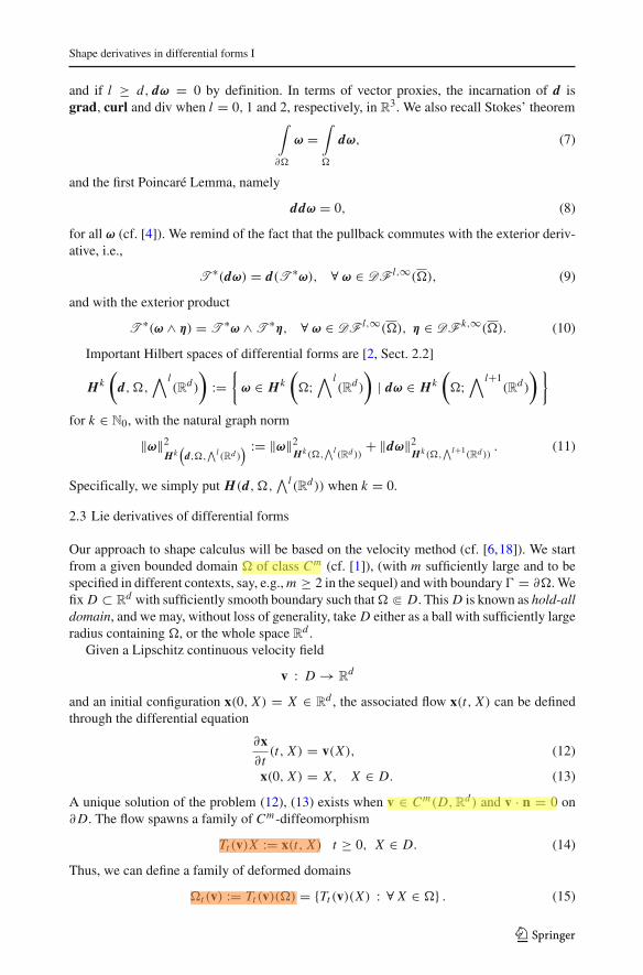
Differential forms can be represented by their coefficient functions, or vector proxies.Please see Table 1 (cf. [13, Section 2.1] and [2, Sect. 2.1]) for vector proxies of differentialforms of different orders in three-dimensional Euclidean space and refer to Table 2 (cf. [8,Chapter 3]) for the interpretation of integrals of differential forms in terms of integrals ofvector proxies.

The exterior product of differential forms ω ∈ DF l,m(!) and η ∈ DF k,m(!) (cf. [4, p.19]),and contraction of ω ∈ DF l,m(!) with a vector field v ∈ Rd (cf. [8, Sect. 2.9.]) aredenoted, respectively, as

ω ∧ η ∈ DF l+k,m(!), ivω ∈ DF l−1,m(!). (3)

1 We adopt the convention that roman letters denote scalar quantities, functions, and their associated spacesetc., while boldface letters represent vector-valued quantities, functions, and their associated spaces etc. Inparticular, boldface Greek letters, ω, η, ν and ρ etc., are reserved for differential forms.

123

R. Hiptmair, J. Li

Table 1 Relationship between differential forms and vector proxies in three-dimensional Euclidean spacev, v1, v2, v3 ∈ R3

Differential form Related function u/vector field u

l = 0 x )→ ω(x) u(x) := ω(x)

l = 1 x )→ {v )→ ω(x)(v)} ⟨u(x), v⟩ := ω(x)(v)

l = 2 x )→ {v1, v2 )→ ω(x)(v1, v2)} ⟨u(x), v1 × v2⟩ := ω(x)(v1, v2)

l = 3 x )→ {v1, v2, v3 )→ ω(x)(v1, v2, v3)} u(x) det(v1, v2, v3) := ω(x)(v1, v2, v3)

Table 2 Relationship between integrals of differential forms and vector proxies in R3

Integral of differential forms Integral of related function u/vector field u

l = 0∫

P ω∫

P u dx := u(P)

l = 1∫

E ω∫

E u · d−→l :=

∫E u · t dl

l = 2∫

F ω∫

F u · d−→S :=

∫F u · n dS

l = 3∫

V ω∫

V u dV

P , E, F, V denotes some point, oriented curve, oriented face and volume in R3 with t and n being the unittangential vector along E and the unit normal vector on F , respectively, and u(P) means point evaluation ofu at P

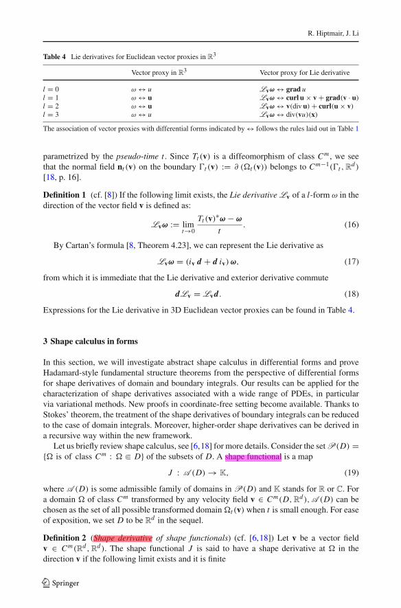
Table 3 Relationship between contraction for differential forms and vector proxies in R3

Contraction of differential forms Contraction of related function u/vector field u

l = 0 x )→ ivω 0 := ivω(x)

l = 1 x )→ ivω(x) (u · v) (x) := ivω(x)

l = 2 x )→ {v )→ ivω(x)(v)} (u × v) (x) := ivω(x)(v)

l = 3 x )→ {v1, v2 )→ ivω(x)(v1, v2)} det(u(x)v, v1, v2) := ivω(x)(v1, v2)

Table 3 gives the operation of contraction for vector proxies in three-dimensional Euclideanspace.

If T : ! )→ ! is a diffeomorphism between two smooth manifolds in Rd , then thepullback T ∗ : DF l,∞(!) )→ DF l,∞(!) [4, p. 28] is given by

((T ∗ω)(x))(v1, . . . , vl) = (ω(T (x)))(DT (x)v1, . . . , DT (x)vl), (4)

where v1, . . . , vl ∈ Rd and the linear map DT (x) : Rd )→ Rd is the derivative (Jacobian)of T at x. The pullbacks satisfy the transformation rule

∫

T (!)

ω =∫

!

T ∗ω. (5)

For a differential l-formω = ∑I ωI dxI ∈ DF l,∞(!), its exterior derivative dω through

the exterior differential operator d [4, p. 20] is defined by

dω :=d∑

i=1

∑

I

∂ωI

∂xidxi ∧ dxI ∈ DF l+1,∞(!), (6)

123

Shape derivatives in differential forms I

and if l ≥ d, dω = 0 by definition. In terms of vector proxies, the incarnation of d isgrad, curl and div when l = 0, 1 and 2, respectively, in R3. We also recall Stokes’ theorem

∫

∂!

ω =∫

!

dω, (7)

and the first Poincaré Lemma, namely

ddω = 0, (8)

for all ω (cf. [4]). We remind of the fact that the pullback commutes with the exterior deriv-ative, i.e.,

T ∗(dω) = d(T ∗ω), ∀ ω ∈ DF l,∞(!), (9)

and with the exterior product

T ∗(ω ∧ η) = T ∗ω ∧ T ∗η, ∀ ω ∈ DF l,∞(!), η ∈ DF k,∞(!). (10)

Important Hilbert spaces of differential forms are [2, Sect. 2.2]

Hk(

d,!,∧l

(Rd)

):=

{ω ∈ Hk

(!;

∧l(Rd)

)| dω ∈ Hk

(!;

∧l+1(Rd)

) }

for k ∈ N0, with the natural graph norm

∥ω∥2Hk

(d,!,

∧l (Rd )) := ∥ω∥2

Hk (!,∧l (Rd ))

+ ∥dω∥2Hk (!,

∧l+1(Rd )). (11)

Specifically, we simply put H(d,!,∧l(Rd)) when k = 0.

2.3 Lie derivatives of differential forms

Our approach to shape calculus will be based on the velocity method (cf. [6,18]). We startfrom a given bounded domain ! of class Cm (cf. [1]), (with m sufficiently large and to bespecified in different contexts, say, e.g., m ≥ 2 in the sequel) and with boundary $ = ∂!. Wefix D ⊂ Rd with sufficiently smooth boundary such that ! ! D. This D is known as hold-alldomain, and we may, without loss of generality, take D either as a ball with sufficiently largeradius containing !, or the whole space Rd .

Given a Lipschitz continuous velocity field

v : D → Rd

and an initial configuration x(0, X) = X ∈ Rd , the associated flow x(t, X) can be definedthrough the differential equation

∂x∂t

(t, X) = v(X), (12)

x(0, X) = X, X ∈ D. (13)

A unique solution of the problem (12), (13) exists when v ∈ Cm(D, Rd) and v · n = 0 on∂ D. The flow spawns a family of Cm-diffeomorphism

Tt (v)X := x(t, X) t ≥ 0, X ∈ D. (14)

Thus, we can define a family of deformed domains

!t (v) := Tt (v)(!) = {Tt (v)(X) : ∀ X ∈ !} . (15)

123

R. Hiptmair, J. Li

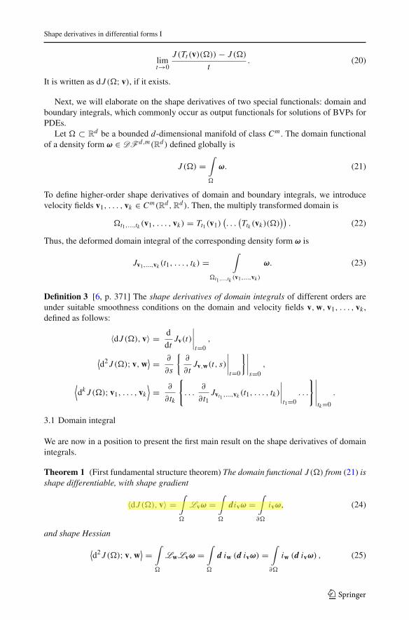
Table 4 Lie derivatives for Euclidean vector proxies in R3

Vector proxy in R3 Vector proxy for Lie derivative

l = 0 ω ↔ u Lvω ↔ grad ul = 1 ω ↔ u Lvω ↔ curl u × v + grad(v · u)l = 2 ω ↔ u Lvω ↔ v(div u) + curl(u × v)l = 3 ω ↔ u Lvω ↔ div(vu)(x)

The association of vector proxies with differential forms indicated by ↔ follows the rules laid out in Table 1

parametrized by the pseudo-time t . Since Tt (v) is a diffeomorphism of class Cm , we seethat the normal field nt (v) on the boundary $t (v) := ∂ (!t (v)) belongs to Cm−1($t , Rd)

[18, p. 16].

Definition 1 (cf. [8]) If the following limit exists, the Lie derivative Lv of a l-form ω in thedirection of the vector field v is defined as:

Lvω := limt→0

Tt (v)∗ω − ω

t. (16)

By Cartan’s formula [8, Theorem 4.23], we can represent the Lie derivative as

Lvω = (iv d + d iv)ω, (17)

from which it is immediate that the Lie derivative and exterior derivative commute

dLv = Lvd. (18)

Expressions for the Lie derivative in 3D Euclidean vector proxies can be found in Table 4.

3 Shape calculus in forms

In this section, we will investigate abstract shape calculus in differential forms and proveHadamard-style fundamental structure theorems from the perspective of differential formsfor shape derivatives of domain and boundary integrals. Our results can be applied for thecharacterization of shape derivatives associated with a wide range of PDEs, in particularvia variational methods. New proofs in coordinate-free setting become available. Thanks toStokes’ theorem, the treatment of the shape derivatives of boundary integrals can be reducedto the case of domain integrals. Moreover, higher-order shape derivatives can be derived ina recursive way within the new framework.

Let us briefly review shape calculus, see [6,18] for more details. Consider the set P(D) ={! is of class Cm : ! ! D} of the subsets of D. A shape functional is a map

J : A (D) → K, (19)

where A (D) is some admissible family of domains in P(D) and K stands for R or C. Fora domain ! of class Cm transformed by any velocity field v ∈ Cm(D, Rd), A (D) can bechosen as the set of all possible transformed domain !t (v) when t is small enough. For easeof exposition, we set D to be Rd in the sequel.

Definition 2 (Shape derivative of shape functionals) (cf. [6,18]) Let v be a vector fieldv ∈ Cm(Rd , Rd). The shape functional J is said to have a shape derivative at ! in thedirection v if the following limit exists and it is finite

123

Shape derivatives in differential forms I

limt→0

J (Tt (v)(!)) − J (!)

t. (20)

It is written as dJ (!; v), if it exists.

Next, we will elaborate on the shape derivatives of two special functionals: domain andboundary integrals, which commonly occur as output functionals for solutions of BVPs forPDEs.

Let ! ⊂ Rd be a bounded d-dimensional manifold of class Cm . The domain functionalof a density form ω ∈ DF d,m(Rd) defined globally is

J (!) =∫

!

ω. (21)

To define higher-order shape derivatives of domain and boundary integrals, we introducevelocity fields v1, . . . , vk ∈ Cm(Rd , Rd). Then, the multiply transformed domain is

!t1,...,tk (v1, . . . , vk) = Tt1(v1)(. . .

(Ttk (vk)(!)

)). (22)

Thus, the deformed domain integral of the corresponding density form ω is

Jv1,...,vk (t1, . . . , tk) =∫

!t1,...,tk (v1,...,vk )

ω. (23)

Definition 3 [6, p. 371] The shape derivatives of domain integrals of different orders areunder suitable smoothness conditions on the domain and velocity fields v, w, v1, . . . , vk ,defined as follows:

⟨dJ (!), v⟩ = ddt

Jv(t)∣∣∣∣t=0

,

⟨d2 J (!); v, w

⟩= ∂

∂s

{∂

∂tJv,w(t, s)

∣∣∣∣t=0

}∣∣∣∣s=0

,

⟨dk J (!); v1, . . . , vk

⟩= ∂

∂tk

{

. . .∂

∂t1Jvt1 ,...,vk (t1, . . . , tk)

∣∣∣∣t1=0

. . .

}∣∣∣∣∣tk=0

.

3.1 Domain integral

We are now in a position to present the first main result on the shape derivatives of domainintegrals.

Theorem 1 (First fundamental structure theorem) The domain functional J (!) from (21) isshape differentiable, with shape gradient

⟨dJ (!), v⟩ =∫

!

Lvω =∫

!

divω =∫

∂!

ivω, (24)

and shape Hessian

⟨d2 J (!); v, w

⟩=

∫

!

LwLvω =∫

!

d iw (d ivω) =∫

∂!

iw (d ivω) , (25)

123

R. Hiptmair, J. Li

and kth order shape derivatives (k > 2)⟨dk J (!); v1, . . . , vk

⟩=

∫

!

(Lvk . . . Lv1

)ω =

∫

!

d ivk

(d ivk−1

(· · ·

(d iv1ω

)))

=∫

∂!

ivk

(d ivk−1 · · ·

(d iv1ω

)). (26)

Proof We first use the pullback to transform from !t to ! and make use of the definition ofthe Lie derivative of a density form ω. Then, we obtain

⟨dJ (!), v⟩ = ddt

Jv(t)∣∣∣∣t=0

=

⎛

⎜⎝ddt

∫

!t (v)

ω

⎞

⎟⎠

∣∣∣∣∣∣∣t=0

=

⎛

⎜⎝ddt

∫

Tt (v)(!)

ω

⎞

⎟⎠

∣∣∣∣∣∣∣t=0

=

⎛

⎝ ddt

∫

!

Tt (v)∗ω

⎞

⎠

∣∣∣∣∣∣t=0

⟨∗⟩=∫

!

Lvω(17)=

∫

!

(d iv + ivd)ω

(8)=∫

!

d ivω(7)=

∫

∂!

ivω,

where the definition of the Lie derivative is used in step ⟨∗⟩. We have also used the factdω = 0 since dω is a (d + 1)-form on a d-dimensional manifold.

Similar manipulations yield the shape Hessian,

⟨d2 J (!), v, w

⟩= ∂

∂s

{∂

∂tJv,w(t, s)

∣∣∣∣t=0

}∣∣∣∣s=0

= ∂

∂s

⎛

⎜⎝

⎛

⎜⎝∂

∂t

∫

!t,s (v,w)

ω

⎞

⎟⎠

∣∣∣∣∣∣∣t=0

⎞

⎟⎠

∣∣∣∣∣∣∣s=0

= ∂

∂s

⎛

⎝

⎛

⎝ ∂

∂t

∫

!

Ts(w)∗Tt (v)∗ω

⎞

⎠

∣∣∣∣∣∣t=0

⎞

⎠

∣∣∣∣∣∣s=0

⟨∗⟩=∫

!

Lw (Lvω)(17)=

∫

!

(d iw + iwd)(d iv + ivd)ω

(8)=∫

!

d iw (d ivω)(7)=

∫

∂!

iw (d ivω) .

Furthermore, for higher-order shape derivatives, we arrive at the last conclusion (26) byrecursively repeating the previous arguments. ⊓3

In particular, regarding the structure of the shape Hessian, due to the composition of con-secutive transformations of ! along velocity fields v and w, the Lie bracket comes into play.Observing (25), we have

⟨d2 J (!), v, w

⟩=

∫

!

LwLvω and⟨d2 J (!), w, v

⟩=

∫

!

LvLwω, (27)

123

Shape derivatives in differential forms I

and in light of the Lie derivative identity [4,7,15]

LwLvω − LvLwω = L[w,v]ω, (28)

where for two differentiable velocity fields, the Lie bracket is defined by [8, Sect. 4]

[w, v] = (Dv) w − (Dw) v, (29)

with Dv, Dw being the Jacobians of the vector fields v and w, respectively. Thus, we arriveat the following symmetry condition, which was also found in [3,5,6] via vector calculus.

Corollary 1 A sufficient condition for the symmetry of the shape Hessian of the domainintegral (21), namely

⟨d2 J (!), v, w

⟩=

⟨d2 J (!), w, v

⟩, (30)

is∫

!

L[w,v]ω = 0. (31)

3.2 Boundary integrals

The boundary functional of a surface density form η ∈ DF d−1,m(D) (initially globallydefined on D) is

I ($) =∫

∂!

η. (32)

Thanks to the Stokes theorem, we see that I ($) =∫! dη. Thus, the structure theorem for

boundary integrals immediately follows from Theorem 1 via the Stokes theorem and the factthat the exterior derivative and Lie derivative commute.

Corollary 2 (Second fundamental structure theorem) The boundary functional I ($) is shapedifferentiable under suitable smoothness conditions on the domain and the velocity fieldsv1, . . . , vk , with shape derivatives for k ≥ 1

⟨dk I ($), v1, . . . , vk

⟩=

∫

$

ivk d(ivk−1 d . . .

(iv1 d (η)

)). (33)

Obviously, only the values of η on $ matter for the shape derivatives. As regards thestructure of the shape Hessian of the boundary integral (32), a result similar to Corollary 1involving the Lie bracket holds. Observe

⟨d2 I ($), v, w

⟩=

∫

!

LwLvdη and⟨d2 I ($), w, v

⟩=

∫

!

LvLwdη. (34)

Therefore, the symmetry condition for the shape Hessian of boundary integrals is∫

$

L[w,v]η = 0, (35)

which is the same as in Corollary 1 except for the domain of integration $.

123

R. Hiptmair, J. Li

3.3 Shape derivative for bilinear forms

For PDE-constrained shape optimization problems, bilinear forms often arise in the varia-tional formulation of the PDE constraints, which have to be differentiated with respect tosmall domain variations. This is the reason why we single out this particular functional.

Lemma 1 For two l-forms, ω, η ∈ DF l,m(!) (0 ≤ l ≤ d − 1), the bilinear form given by

J (!) =∫

!

∗dω ∧ dη, (36)

where ∗ is the Hodge star operator (cf. [4,7,8]), has the following shape derivative:

⟨dJ (!), v⟩ =∫

!

Lv (∗dω ∧ dη) =∫

$

iv (∗dω ∧ dη) . (37)

Proof Understanding ∗dω ∧ dη as a density form, the assertion follows directly fromTheorem 1. ⊓3

4 Shape calculus in vector proxies

In this section, we will express the abstract theory in Sect. 3 in terms of vector proxies ind-dimensional Euclidean space (cf. Table 1).

For later use, we introduce surface differential operators as follows: Let u (resp. v) be theclassical extension of some scalar function u (resp. vector fields v) on the surface $ to thewhole space Rd by means of the signed smooth distance function within some neighborhoodof $ [6,16,19]. Then, two key surface differential operators can be defined,

Surface gradient : grad$ u = grad u|$ − (grad u · n) n|$,

Surface divergence : div$v = div v − Dvn · n,

with n being the outward unit normal vector on $. They are linked by the tangential Stokesand Green Formulae on the hypersurface $ of codimension one without boundary in Rd [6,Eqs. (5.26) and (5.27) on p. 367]: For a function f ∈ C1($) and a vector v ∈

(C1($)

)d , wehave the tangential Stokes formula

∫

$

div$v ds =∫

$

Hv · n ds, (38)

and the tangential Green formula∫

$

f div$v + grad$ f · v ds =∫

$

H f v · n ds, (39)

where

H := (d − 1)H (40)

is the additive curvature and H is the mean curvature of the surface $ (cf. [6]).

123

Shape derivatives in differential forms I

4.1 Domain integrals

Given a sufficiently smooth function f and a smooth domain ! of class Cm with boundary$, the domain integral functional is

J (!) =∫

!

f dx . (41)

In terms of vector proxies in Euclidean space, see Table 1, and understanding f as vectorproxy for a d-dimensional volume form ω ∈ DF d,m(!), the formulae in Theorem 1 can berecast as follows:

Lemma 2 Under suitable smoothness conditions on f,! and the velocity fields v and w,the shape gradient of J from (41) exists and can be written as:

⟨dJ (!), v⟩ =∫

$

( f v) · n ds.

The shape Hessian is

⟨d2 J (!), v, w

⟩=

∫

$

(∂ f∂n

+ κ f)

(v · n) (w · n) ds

−∫

$

f(⟨Sv$, w$⟩ − w$ · grad$ (v · n) − v$ · grad$ (w · n)

)ds

+∫

$

f (Dvw) · n ds, (42)

where S = Dn is the second fundamental form (or Weingarten map or shape operator [8,17])of the surface $ and n is the outward unit normal field on $.

Proof The scalar smooth function f can be viewed as a vector proxy of a density form. Sincethe contraction with a velocity field amounts to a simple product of a scalar function f and avector field (see Table 3), and the exterior derivative d is nothing but the div operator in thiscase, following (24) in Theorem 1, the shape gradient of (41) reads:

⟨dJ (!), v⟩ =∫

!

div( f v) dx =∫

$

( f v) · n ds.

This formula agrees with [18, Proposition 2.4.6 on p. 77] or [6, Theorem 4.2, p. 353].The shape Hessian can be derived from (25) in a similar way, we obtain

⟨d2 J (!), v, w

⟩=

∫

!

div (w div( f v)) dx =∫

$

div( f v) (w · n) dx

=∫

$

(grad f · v + f div v) (w · n) ds

⟨4⟩=∫

$

(grad$ f · v$ + ∂ f

∂nv · n + f (Dvn · n + div$v)

)(w · n) ds

123

R. Hiptmair, J. Li

⟨5⟩=∫

$

(grad$ f · v$ +

(∂ f∂n

+ H f)

v · n + f Dvn · n + f div$ v$

)

× (w · n) ds⟨6⟩=

∫

$

((∂ f∂n

+ H f)

v · n + f Dvn · n)

(w · n) − f v$ · grad$ (w · n) ds

(43)

Note that H is the additive mean curvature defined in (40). Here we have used the decompo-sition

v = (v · n)n + v$, (44)

where (·)$ denotes the tangential component of a vector field on $, and the definition ofsurface divergence

div v = Dvn · n + div$v, (45)

cf. [18, Def. 2.52, p. 82] or [6, Eq. (5.19), p. 366], in the fourth equality ⟨4⟩. The fifth equality⟨5⟩ follows from the identity

div$v = div$v$ + Hv · n, (46)

(cf. [18, Prop. 2.57, p. 86] or [6, Eq. (5.22), p. 366]). And the last equality ⟨6⟩ is a consequenceof the tangential Green formula (39) applied to v$ and (w · n) f :

∫

$

grad$ ((w · n) f ) · v$ + (w · n) f div$ v$ ds = 0. (47)

Note that the formula (43) is exactly the same as [6, Eq.(6.3) on p. 373]. However, we avoida lot of complicated intermediate steps and need not introduce some auxiliary distance func-tions and surface calculus. Moreover, in light of [6, Eq. (5.23) on p. 366], one may furthersymmetrize the shape Hessian in (43) as [6, Eq. (6.4) on p. 373] to derive a symmetric prin-cipal part plus the first half of the Lie bracket of two velocity fields to obtain (42). Thiscompletes the proof. ⊓3

In terms of a vector proxy f of a density form, the sufficient condition from Corollary 1for the symmetry of the shape Hessian is equivalent to

∫

!

div ( f [w, v]) dx =∫

∂!

( f [w, v]) · n ds =∫

∂!

f ((Dv) w − (Dw) v) · n ds = 0,

which agrees with the observation in [6, Eq. (6.5) on p. 373]. Related investigations of thestructure of the shape Hessian of domain integrals can be found in [3,5].

Remark 1 In particular for shape optimization problems, only normal variations (still pertur-bations of infinite dimension) are taken into account, namely v and w are chosen to be alongthe normal direction of the surface $. In such a case, the symmetry of the shape Hessianis still not guaranteed from the velocity method, which is quite opposite to our intuition offinite dimensional calculus. So one should be very cautious about assuming the symmetry ofthe shape Hessian in shape optimization problems.

123

Shape derivatives in differential forms I

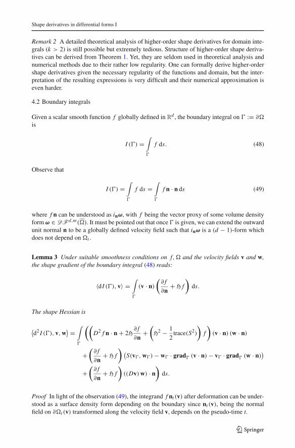
Remark 2 A detailed theoretical analysis of higher-order shape derivatives for domain inte-grals (k > 2) is still possible but extremely tedious. Structure of higher-order shape deriva-tives can be derived from Theorem 1. Yet, they are seldom used in theoretical analysis andnumerical methods due to their rather low regularity. One can formally derive higher-ordershape derivatives given the necessary regularity of the functions and domain, but the inter-pretation of the resulting expressions is very difficult and their numerical approximation iseven harder.

4.2 Boundary integrals

Given a scalar smooth function f globally defined in Rd , the boundary integral on $ := ∂!

is

I ($) =∫

$

f ds. (48)

Observe that

I ($) =∫

$

f ds =∫

$

f n · n ds (49)

where f n can be understood as inω, with f being the vector proxy of some volume densityform ω ∈ DF d,m(!). It must be pointed out that once $ is given, we can extend the outwardunit normal n to be a globally defined velocity field such that inω is a (d − 1)-form whichdoes not depend on !t .

Lemma 3 Under suitable smoothness conditions on f,! and the velocity fields v and w,the shape gradient of the boundary integral (48) reads:

⟨dI ($), v⟩ =∫

$

(v · n)

(∂ f∂n

+ H f)

ds.

The shape Hessian is

⟨d2 I ($), v, w

⟩=

∫

$

((D2 f n · n + 2H

∂ f∂n

+(

H2 − 12

trace(S2)

)f)

(v · n) (w · n)

+(

∂ f∂n

+ H f) (

S(v$, w$) − w$ · grad$ (v · n) − v$ · grad$ (w · n))

+(

∂ f∂n

+ H f)

((Dv) w) · n)

ds.

Proof In light of the observation (49), the integrand f nt (v) after deformation can be under-stood as a surface density form depending on the boundary since nt (v), being the normalfield on ∂!t (v) transformed along the velocity field v, depends on the pseudo-time t.

123

R. Hiptmair, J. Li

Now interpreting d as div and contraction as simple multiplication, we have

⟨dI ($), v⟩ =∫

$

div( f n)(v · n) ds

︸ ︷︷ ︸I

+ 2∫

$

f (n′t (v)|t=0) · n ds

︸ ︷︷ ︸I I

=∫

$

(grad f · n + f div(n)) (v · n) ds

=∫

$

(v · n)

(∂ f∂n

+ H f)

ds. (50)

where we have to apply the product rule of differentiation to the boundary integral (49).The first term (I ) follows from Corollary 2 through freezing n = nt (v)|t=0 and extending itunitarily to the global domain by the signed distance technique, while the second one (I I )is a temporal derivative of the integrand f nt (v) · nt (v) evaluating at t = 0. Notice that

n′t (v)|t=0 = − grad$(v · n), (51)

which is a tangential vector on the surface $ (please refer to details in [6, Eq. (4.38) on p.360 and p. 370]. Therefore, we see immediately that (I I ) vanishes.

In the derivation of the previous formula (50), we have used the identities

div( f n) = grad( f ) · n + f div(n)

and div(n) = Trace(Dn) = H. This formula agrees with [6, Theorem 4.3 on p. 355], but wecould arrive at it much more easily.

As for the shape Hessian, we may repeat the argument in the derivation of the shapegradient recursively and thus obtain from Corollary 2

⟨d2 I ($), v, w

⟩=

∫

$

div (v div( f n)) (w · n) ds

=∫

$

div (v (grad( f ) · n + f div(n))) (w · n) ds

=∫

$

(div v (grad( f ) · n + f div(n))

+ grad (grad( f ) · n + H f ) · v)(w · n) ds.

We point out that we have used the product rule of differentiation and the orthogonality(51) twice in pseudo-time s and t consecutively in deriving the shape Hessian for boundaryintegrals. To the best knowledge of the authors, this is a new result.

123

Shape derivatives in differential forms I

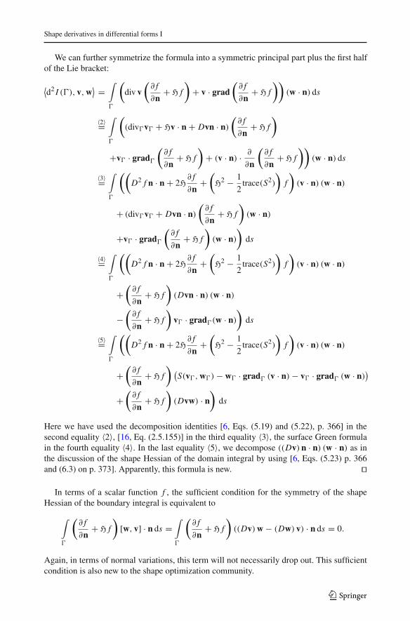
We can further symmetrize the formula into a symmetric principal part plus the first halfof the Lie bracket:

⟨d2 I ($), v, w

⟩=

∫

$

(div v

(∂ f∂n

+ H f)

+ v · grad(

∂ f∂n

+ H f))

(w · n) ds

⟨2⟩=∫

$

((div$v$ + Hv · n + Dvn · n)

(∂ f∂n

+ H f)

+v$ · grad$

(∂ f∂n

+ H f)

+ (v · n) · ∂

∂n

(∂ f∂n

+ H f))

(w · n) ds

⟨3⟩=∫

$

((D2 f n · n + 2H

∂ f∂n

+(

H2 − 12

trace(S2)

)f)

(v · n) (w · n)

+ (div$v$ + Dvn · n)

(∂ f∂n

+ H f)

(w · n)

+v$ · grad$

(∂ f∂n

+ H f)

(w · n)

)ds

⟨4⟩=∫

$

((D2 f n · n + 2H

∂ f∂n

+(

H2 − 12

trace(S2)

)f)

(v · n) (w · n)

+(

∂ f∂n

+ H f)

(Dvn · n) (w · n)

−(

∂ f∂n

+ H f)

v$ · grad$(w · n)

)ds

⟨5⟩=∫

$

((D2 f n · n + 2H

∂ f∂n

+(

H2 − 12

trace(S2)

)f)

(v · n) (w · n)

+(

∂ f∂n

+ H f) (

S(v$, w$) − w$ · grad$ (v · n) − v$ · grad$ (w · n))

+(

∂ f∂n

+ H f)

(Dvw) · n)

ds

Here we have used the decomposition identities [6, Eqs. (5.19) and (5.22), p. 366] in thesecond equality ⟨2⟩, [16, Eq. (2.5.155)] in the third equality ⟨3⟩, the surface Green formulain the fourth equality ⟨4⟩. In the last equality ⟨5⟩, we decompose ((Dv) n · n) (w · n) as inthe discussion of the shape Hessian of the domain integral by using [6, Eqs. (5.23) p. 366and (6.3) on p. 373]. Apparently, this formula is new. ⊓3

In terms of a scalar function f , the sufficient condition for the symmetry of the shapeHessian of the boundary integral is equivalent to

∫

$

(∂ f∂n

+ H f)

[w, v] · n ds =∫

$

(∂ f∂n

+ H f)

((Dv) w − (Dw) v) · n ds = 0.

Again, in terms of normal variations, this term will not necessarily drop out. This sufficientcondition is also new to the shape optimization community.

123

R. Hiptmair, J. Li

4.3 Shape derivative for bilinear forms

The formula in (37) holds true for grad, curl and div, respectively, in three dimensions.These special cases can be summarized in the following version of Lemma 1.

Lemma 4 Under suitable smoothness conditions on ! and the velocity field v, the shapederivatives of the bilinear form on H(D,!)

J (!) =∫

!

κDu · Dv dx, (52)

is

⟨dJ (!), v⟩ =∫

$

(κDu · Dv) v · n ds, (53)

with D being replaced with grad, curl and div, respectively, u and v vector fields for thelatter two cases, and κ some coefficient, which could be any constant, smooth function ortensor field.

Note that those formulae for curl and div operators are new and of particular importancein deriving shape derivatives for Maxwell solutions arising in electromagnetics, and for theStokes system arising in fluid dynamics, respectively.

4.4 Normal derivative

Since normal derivatives are often encountered, we would like to discuss this special casewith an auxiliary lemma. Let $ be the boundary of a bounded domain ! of class Cm andf ∈ H2

loc(Rm) be given. Consider the shape functional

I ($) =∫

$

∂ f∂n

ds =∫

$

grad f · n ds. (54)

In this case, f is understood as a 0-form ω and grad is the incarnation of d : DF 0,m(!) )→DF 1,m(!), thus

∫$ grad f ·n ds may be expressed by

∫$ ∗dω, where dω is a 1-form, which

is mapped by the Euclidean Hodge to ∗dω, a (d − 1)-form (or grad f in the vector proxy).Now Corollary 2 is applicable for this case.

Lemma 5 Under suitable smoothness conditions on ! and the velocity fields v, the shapederivative of (54) exists and it holds that

⟨

d∫

$

grad f · n, v

⟩

(55)

=∫

$

(div$ grad$ f + D2 f n · n + H grad f · n

)(v · n) ds. (56)

123

Shape derivatives in differential forms I

Proof By Corollary 2, we have⟨

d∫

$

grad f · n, v

⟩

=∫

$

div(grad f ) (v · n) ds

=∫

$

(div$ grad$ f + D2 f n · n + H grad f · n

)(v · n) ds.

where we have used the decomposition of the div operator as in (45) and (46) in the secondequality. ⊓3

5 Application: shape derivative of solutions of second-order BVPs

In this section, we will study a model elliptic BVP and express the shape derivatives of weaksolutions of BVPs via shape calculus of domain and boundary integrals.

Given a bounded domain ! ⊂ Rd of class Cm , consider an elliptic BVP for an l-form ω,see [12, Sect. 2],

(−1)d−l d ∗α dω + ∗γω = ψ in !, (57)

Tr (∗αdω) = (−1)d−lTr(∗βω + φ

)on $, (58)

where ∗α, ∗γ and ∗β are fixed Hodge operators in ! and on $, respectively, Tr is the traceoperator on the boundary [2], andψ ((d − l)-form) and φ ((d − l − 1)-form) are two smoothdifferential forms defined globally. Equation (58) corresponds to the Robin boundary condi-tion, which reduces to the Neumann case when ∗β = 0.

The weak form of (57), (58) is obtained through the integration by parts formula [13, Eq.(2.23)] and reads: Seek ω ∈ {η ∈ H(d,!,

∧l(Rd)), Tr(η) ∈ L2($,∧l(Rd))} such that for

all smooth test forms η∫

!

(∗αdω ∧ dη + ∗γω ∧ η

)+

∫

$

Tr(∗βω ∧ η

)=

∫

!

ψ ∧ η −∫

$

Tr (φ ∧ η) . (59)

Definition 4 (Shape derivatives of forms) Given a velocity field v ∈ Cm(Rd , Rd) and thecorresponding perturbed domains !t := Tt (v)(!), the shape derivatives of a solution ω of(57), (58), which depends on the domain !t , in the direction of v, denoted by δω, is definedby (cf. [6,18])

δω := ddtω(!t )

∣∣∣∣t=0

. (60)

In an abstract way, we can characterize the corresponding shape derivative of the solutionto (57), (58) by differentiating (59) with respect to t , but with ! and ω(!) replaced by !tand ω(!t ) in (59), respectively. Straightforward application of Theorem 1, Corollary 2 andDefinition 4 yields:

Lemma 6 The shape derivative, δω ∈ {η ∈ H(d,!,∧l(Rd)) : Tr(η) ∈ L2($,

∧l(Rd))},of the solution ω ∈ H1

(d,!,

∧l(Rd))

of (59) is the unique solution to the followingvariational problem:

123

R. Hiptmair, J. Li

∫

!

(∗αd(δω) ∧ dη + ∗γ δω ∧ η

)+

∫

$

Tr(∗βδω

)∧ η.

=∫

$

iv (ψ ∧ η) −∫

$

iv(∗αdω ∧ dη + ∗γω ∧ η

)

−∫

$

ivdTr((

∗βω + φ)∧ η

), (61)

for all smooth test forms η ∈ DF l,∞(Rd).

The weak form (59) corresponds to H1(!)-, H(curl;!)- and H(div;!)-elliptic varia-tional problems when d = 3, l = 0, 1 and 2, respectively. In terms of vector proxies, we canincarnate the Hodge operators as multiplication with coefficient functions denoted by α,β

and γ .We give details for 0-forms (l = 0, for l > 0, please refer to [14]), and use scalar functions

f ∈ L2(!) and g ∈ H2(!) as vector proxies of the forms ψ and φ in (59). Related studieshave been conducted in [10,11,18].

Corollary 3 The shape derivative, δu ∈{w ∈ H1(!) : w|∂! ∈ H1($)

}, of the solution

u ∈ H2(!) of (59) for l = 0 is the unique solution of the following variational problem:∫

!

(α grad δu · grad v + γ δuv) +∫

$

βδu

=∫

$

f vv · n −∫

$

(α grad$ u · grad$ v + γ uv

)v · n

−∫

$

v · n(

∂

∂n(βu + g) + H(βu + g)

)v, (62)

for all v ∈ C∞(Rd).

Proof A simple translation from differential forms to scalar functions (0-forms) with Lemmas2 and 3 yields the right-hand side of (61) in terms of vector proxies∫

$

f vv · n−∫

$

(α grad u · grad v+γ uv) v · n−∫

$

v · n(

∂

∂n((βu + g)v)+H(βu + g)v

).

Notice that

∂

∂n((βu + g)v) = ∂

∂n(βu + g) v + (βu + g)

∂v

∂n,

and

α grad u · grad v = α grad$ u · grad$ v + α∂u∂n

· ∂v

∂n.

In view of the Robin boundary condition α ∂u∂n + (βu + g) = 0, the last terms in the previous

two equations cancel each other and the proof is done. ⊓3

123

Shape derivatives in differential forms I

Once we arrive at the variational characterization of the shape derivative, we can reformu-late the strong form of the PDE for the shape derivative δu under suitable regularity conditionsby testing (62) first with smooth functions v with vanishing trace, and, subsequently, withsmooth functions v with non-zero trace. The strong form of (62) follows from (39):

− div (α grad δu) + γ δu = 0 in !, (63)

α∂ (δu)

∂n+ βδu = div$

((v · n)α grad$ u

)

−v · n(

∂(βu + g)

∂n+ H(βu + g)

)+ ( f − γ u)v · n on $. (64)

Thus, we obtain the elliptic BVP for the shape derivative δu and its associated Robin boundarycondition (or its Neumann counterpart when β = 0).

6 Dual formulation

For PDEs with Neumann or Robin boundary conditions, it is natural to derive the correspond-ing Neumann or Robin boundary conditions of the shape gradient of solutions to the PDEsfrom its primal variational formulation. In this section, we will rigorously derive the shapederivative for BVPs with Dirichlet boundary condition from the dual variational formulation.The aforementioned elliptic BVP (57) for general l-forms will be further discussed from thedual perspective, but equipped with some Dirichlet boundary condition

ω = φ on $. (65)

To derive the dual formulation, we introduce a (d − l − 1)-form

ρ = ∗αdω, (66)

or

∗α−1 ρ = (−1)(l+1)(d−l−1)dω. (67)

where ∗α−1 , up to sign, is the inverse of the Hodge operator ∗α with ∗α−1 ◦ ∗α =(−1)(l+1)(d−l−1) Id . Then, the PDE (57) can be rewritten as (67) plus

(−1)d−l dρ + ∗γω = ψ in !. (68)

Now the dual mixed formulation of (67) and (68) is as follows:∫

!

∗α−1ρ ∧ τ + (−1)(l+1)(d−l)ω ∧ dτ + (−1)(l+1)(d−l−1)

∫

$

Trφ ∧ Trτ = 0, (69)

∫

!

(−1)(d−l)dρ ∧ ν +∫

!

∗γω ∧ ν =∫

!

ψ ∧ ν, (70)

for all smooth τ ∈ DF d−l−1,∞(Rd) and ν ∈ DF d−l,∞(Rd). Taking the shape derivative ofthe mixed formulation, namely differentiating the above formulation in the perturbed domain!t with respect to the pseudo-time t , we conclude from Theorem 1 and Corollary 2,

123

R. Hiptmair, J. Li

∫

!

∗α−1δρ ∧ τ + (−1)(l+1)(d−l)δω ∧ dτ

+(−1)(l+1)(d−l−1)

∫

$

ivd (Trφ ∧ Trτ )

∫

$

ivTr(∗α−1ρ ∧ τ + (−1)(l+1)(d−l)ω ∧ dτ

)= 0, (71)

∫

!

(−1)(d−l)dδρ ∧ ν +∫

!

∗γ δω ∧ ν

+∫

$

ivTr((−1)(d−l)dρ ∧ ν + ∗γω ∧ ν − ψ ∧ ν

)= 0. (72)

Up to here, we have characterized the shape derivatives δω and δρ of the primal form ωand dual form ρ in the variational sense, which is now amenable to further investigation forconcrete settings.

Here, we discuss the special case l = 0 and, for the sake of simplicity, assume α = 1 and∗γ = 0. The scalar functions f ∈ L2(Rd) and g ∈ H2(Rd) will serve as vector proxies forthe differential forms ψ and φ (57) and (59). Thus, we arrive at the Dirichlet problem

−*u = f on !, u = g in $, (73)

whose dual weak form emerges from setting

q = grad u, (74)

and reads: Seek u ∈ L2(!) and q ∈ H(div;!) such that⎧⎪⎨

⎪⎩

∫

!

q · p dx +∫

!

u div p dx =∫

$

gp · n, ∀ p ∈ H(div;!),

∫

!

div qv dx =∫

!

f v dx, ∀ v ∈ L2(!).(75)

For smooth domains and data, we can expect u ∈ H2(!) and q ∈ H1(div;!). Write δq andδu as the shape derivatives of q and u, respectively, in the direction of some given velocityfield v. Understanding q and u as a (d − 1)-form and a 0-form, respectively, in Rd , andreinterpreting (71) and (72) in terms of vector proxies, we have the variational equation forshape derivatives:

Seek δq ∈ H(div;!) and δu ∈ L2(!) such that for all p ∈ (C∞(!))d and v ∈ C∞(!)

⎧⎪⎪⎪⎪⎨

⎪⎪⎪⎪⎩

∫

!

δq · p dx +∫

!

δu div p dx

+∫

$

v · n (q · p + u div p) ds =∫

$

v · n(

∂(gp·n)∂n + Hgp · n

)ds,

∫

!

div δqv dx +∫

$

v · n (div q − f ) v dx = 0.

(76)

The loss of regularity in δq and δu compared with q and u follows from differentiation withrespect to the domain, in particular due to the weaker regularity of the boundary data.

To determine the boundary condition satisfied by the shape derivative δu, we first test thefirst equation of (76) with p ∈

(C∞

0 (!))d and v ∈ C∞

0 (!) and learn

δq = grad δu. (77)

123

Shape derivatives in differential forms I

Therefore, δu ∈ L2(!) and δq ∈ L2(!) implies δu ∈ H1(!). Next, testing the first equa-tion of (76) with p ∈

(C∞(!)

)dand splitting the third term there in normal and tangential

directions, we see, in light of [6, Eqs. (5.19) and (5.22), p. 366], that

q · p + u div p = (q · n) (p · n) + q$ · p$

+u(Dp)n · n + udiv$p$ + Hup · n. (78)

Noticing by the chain rule that

∂(gp · n)

∂n= ∂g

∂np · n + g(Dp)n · n + g(Dn)p · n. (79)

The last term in (79) vanishes since Dnp = Sp is a tangential vector due to orthogonality ofthe Weingarten map S (cf. [17]). Now straightforward calculation combined with u = g on$, (74) and (39) for q$ · p$ and udiv$p$ yields

∫

$

(δu + v · n

(∂u∂n

− ∂g∂n

))p · n ds = 0. (80)

As p is arbitrary, we immediately have

δu = −(

∂u∂n

− ∂g∂n

)v · n on $ (81)

in the trace space H12 (!), since u and g ∈ H2(!).

7 Conclusion

In the present paper, we have presented shape derivatives from the perspective of differentialforms and shape calculus via exterior calculus of differential forms. This approach is in par-ticular convenient for deriving shape derivatives of solutions of second-order BVPs in bothprimal and dual variational formulation. It reveals the essential structure of shape derivativesin terms of recursive composition of Lie derivatives. Moreover, a sufficient condition for thesymmetry of the second-order shape Hessian is stated in terms of a vanishing Lie bracket.We have demonstrated the power of our approach by illustrating some typical examples likeboundary and domain integrals, bilinear forms and normal derivatives, etc. We have alsotreated a concrete example, a model second-order BVP that covers all kinds of boundaryconditions. For the first time, we show how to derive the boundary condition to the shapederivative of the solution to the PDE with a non-homogeneous Dirichlet boundary conditionvia the dual mixed formulation.

Acknowledgments The authors would like to thank Professor Thorsten Hohage from the universityof Göttingen for providing us his thesis for reference and helpful discussion during his visit at ETH in March2011 and Dr. Holger Heumann from ETH, Zürich for fruitful discussion on the Lie derivative.

References

1. Adams, R.A.: Sobolev Spaces. Academic Press, New York, NY (1975)2. Arnold, D.N., Falk, R.S., Winther, R.: Finite element exterior calculus, homological techniques, and

applications. Acta Numerica 15, 1–155 (2006)

123

R. Hiptmair, J. Li

3. Bucur, D., Zolésio, J.-P.: Anatomy of the shape hessian via lie brackets. Annali di Matematica Pura EdApplicata 173, 127–143 (1997)

4. Cartan, H.: Differential Forms. Hermann, Paris (1970)5. Delfour, M.C., Zolésio, J.P.: Anatomy of the shape hessian. Annali di Matematica Pura Ed Appli-

cata 159, 315–339 (1991)6. Delfour, M.C., Zolésio, J.-P.: Shapes and Geometries: Analysis, Differential Calculus, and Optimiza-

tion. SIAM, Philadelphia (2001)7. Flanders, H.: Differential Forms with Applications to the Physical Sciences. Academic Press, New York,

NY (1963)8. Frankel, T.: The Geometry of Physics: An Introduction. Cambridge University Press, Cambridge (1997)9. Hadamard, J.: Lessons on the Calculus of Variation (in French). Gauthier-Villards, Paris (1910)

10. Hettlich, F.: Frechet derivatives in inverse obstacle scattering. Inverse Probl. 11, 371–382 (1995)11. Hettlich, F.: Frechet derivatives in inverse obstacle scattering. Inverse Probl. 14, 209–210 (1998)12. Hiptmair, R.: Discrete hodge operators. Numer. Math. 90, 265–289 (2001)13. Hiptmair, R.: Finite elements in computational electromagnetism. Acta Numerica 11, 237–339 (2002)14. Hiptmair, R., Li, J.: Shape Derivatives in Differential Forms II: Applications to Acoustic and Electro-

magnetic Scattering Problems. Technical report, SAM, ETH, Zürich, Switzerland (2012, in preparation)15. Kolár, I., Michor, P., Slovák, J.: Natural Operations in Differential Geometry. Springer, Berlin (1993)16. Nédélec, J.-C.: Acoustic and Electromagnetic Equations: Integral Representations for Harmonic Prob-

lems, vol. 144 of Applied Mathematical Sciences. Springer, New York, NY (2001)17. O’Neill, B.: Elementary Differential Geometry, 2nd edn. Academic Press, New York, NY (1997)18. Sokolowski, J., Zolésio, J.-P.: Introduction to Shape Optimization: Shape Sensitivity Analysis. Springer,

Berlin (1992)19. Stein, E.M.: Singular Integrals and Differentiability Properties of Functions. Princeton University

Press, Princeton (1970)

123