Shape Constraints in Economics and Operations Research

Submitted to Statistical Science

Shape Constraints in Economicsand Operations ResearchAndrew L. Johnson and Daniel R. Jiang

Texas A&M University and Osaka UniversityUniversity of Pittsburgh

Abstract. Assumptions motivated by either logical or existing theorycan be imposed during model estimation to restrict the feasible regionof the parameters. The restrictions, implemented as shape constraints,may not provide any benefits in an asymptotic analysis, but will im-prove the estimator’s finite sample performance. This paper briefly re-views an illustrative set of research on shape constrained estimationin the economics and operations research literature. We highlight themethodological innovations and applications, with a particular empha-sis on utility functions, production economics, and sequential decisionmaking applications.

Key words and phrases: Shape Constraints, Multi-variate Convex Re-gression, Nonparametric Regression, Production Economics, ConsumerPreferences, Revealed Preferences, Approximate Dynamic Program-ming, Reinforcement Learning.

1. INTRODUCTION

This paper builds on prior surveys of shape constrained estimation in theeconomics literature by Matzkin (1994), Yatchew (2003), and Chetverikov et al.(2018), and also surveys the operations research literature for the first time.Although length limitations prohibit a comprehensive survey, we describe theimportant central themes and identify the recent advances and applications andactive research directions in the literature.

One of the first papers published in the economics literature is Hildreth (1954)who estimated the relationship between corn output and nitrogen fertilizer re-stricting output to be a function of fertilizer that was monotonically increasingand concave. Later, Brunk (1970) studied isotonic functions, or imposing a mono-tonicity constraint on the function, and showed for isotonic regression with asingle regressor the consistency and the rate of convergence. Barlow et al. (1972)

Andrew Johnson is an Associate Professor in the Department of Industrial andSystems Engineering, Texas A&M University, College Station, Texas 77840,USA, and holds an appointment as a Visiting Associate Professor in School ofInformation Science and Technology, Osaka University, Suita 565-0871, Japan.(e-mail: [email protected]). Daniel Jiang is an Assistant Professor in theDepartment of Industrial Engineering, University of Pittsburgh, Pittsburgh, PA15261, USA. (e-mail: [email protected]).

1imsart-sts ver. 2014/10/16 file: output.tex date: August 29, 2018

http://www.imstat.org/sts/

mailto:[email protected]

mailto:[email protected]

2 JOHNSON AND JIANG

were the first to develop and organize fundamental results in order restrictedinference for isotonic regression. Robertson et al. (1988) summarized one of theearliest conferences on shape constrained functional estimation. Mammen (1991)considered the two-step estimation of a smooth monotone function in a single re-gressor setting and analyzed interchanging the isotonization step and the smooth-ing step. Hall and Huang (2001) considered the estimation of a monotonic andconvex/concave function with a single regressor using kernel weighting methodswith an additional weigh vector to assure the function satisfied the shape con-straints. Villalobos and Wahba (1987), who considered the estimation of a smoothfunction with a set of linear inequality constraints, provided a characterizationwhich could be solved using a nonlinear programming algorithm.

Our survey is divide into a section on regression-based estimation and a sec-tion on sequential decision making. Within the regression-based estimator sec-tion, we divide the relevant research into three subsection: 1) The NonparametricLeast Squares Estimator; 2) Approximate Global Shape Restrictions, Ensem-ble Methods, and Local Weighting; and 3) Single Index Models and AlternativeAssumptions to Global Convexity. In each subsection we describe both a setof estimators and an application that illustrates the estimators. For subsection1) the application is utility function estimation, whereas in subsections 2) and3) the application is production function estimation. In the sequential decisionmaking section, the subsections are 1) Convexity of the Value Function, 2) Mono-tonicity and 3) Policy Structure. Several examples are included throughout thesection. We refer readers interested in other relevant topics and applications ofshape constraint estimation, e.g., option pricing or stochastic approximation tosee Aıt-Sahalia and Duarte (2003) and Kushner and Yin (2003), respectively. Fortesting, we suggest Chernozhukov et al. (2015) and Chetverikov et al. (2018) andthe references therein.

2. REGRESSION-BASED ESTIMATORS

Regression models allow the investigation of observational data to identify cor-relations among variables to provide basic empirical evidence of the relationshipbetween variables. Here we will review several regression based methods for es-timating these relationship while imposing additional information which can bestated as shape constraints on the regression models. We will begin in Section2.1 with the widely used nonparametric least squares estimator (LSE). Estimat-ing the nonparametric LSE with shape constraints results in functional estimatesthat satisfy a set of global axiomatic properties. We will describe the applicationof using Afriat inequalities to test the generalized axioms of revealed preferences.Then in Section 2.2 we will consider approximations to nonparametric estima-tor with globally axiomatic properties. These estimators will approximate eitherthe axioms or the function by only imposing weaker versions of the axiom orby using parametric approximations. In some cases these approximations canbe improved by ensemble methods or local weighting both of which will be dis-cussed. We will discuss applications related to production economics where theseestimators are used. Finally in Section 2.3, we will review single index modelsand alternative shape restrictions. Single index models assure predictor variablesare aggregated to maintain properties such as linearity or convexity while allow-ing the relationship between the dependent variable and the aggregate predictor

imsart-sts ver. 2014/10/16 file: output.tex date: August 29, 2018

SHAPE CONSTRAINTS IN ECONOMICS AND OPERATIONS RESEARCH 3

to remain general. These models can be used to implement more complicatedeconomic models of production where convexity is maintained between certainvariables while more complicated relationships such as the S-shape can be im-posed between other variables. We will illustrate these models with extensionsdeveloped in production economics applications.1

2.1 The Nonparametric Least Squares Estimator

One of the most widely used shape constrained estimators is the nonparamet-ric LSE of a multi-variate convex regression function (Groeneboom et al., 2001;Kuosmanen, 2008; Seijo and Sen, 2011). Initial work on multi-variate convex re-gression functions includes Matzkin (1991), Banker and Maindiratta (1992), andAllon et al. (2007), who considered maximum likelihood estimators. The con-sistency of the first two estimators is shown in Matzkin (1991) and Sarath andMaindiratta (1997), respectively. However, both estimators have had little prac-tical implementation because of the computational complexity of the associatedoptimization problems. Allon et al. (2007) described some of these complexi-ties and used the concept of entropic distance to develop a maximum likelihoodestimator that can be stated as a convex programming problem and thus canbe solved for data sets of up to 400 observations which was considered a largeinstance. Many of the computational strategies for the nonparametric LSE de-scribed below are directly applicable to the Allon estimator, but they have notbeen pursued in the literature. Alternatively, Beresteanu et al. (2007) considereda sieve estimator with a least squares loss function, and evaluated the metricentropy of the space of shape-restricted functions.

Kuosmanen (2008) proposed the characterization of the nonparametric LSEof a multi-variate convex regression function. Unlike the previous estimators,this characterization relaxes assumptions on the distribution of the error termand the need for turning parameters. To define the model, consider the set ofobservations (Xi, Yi) : i = 1, 2, . . . , n and a nonparametric shape restrictedregression satisfying

(2.1) Yi = f(Xi) + εi.

Here, Xi ∈ Rd is an observed vector of predictors where d ≥ 1. The noise term,εi satisfy E(εi |X) = 0, and the real-valued regression function f is unknownbut obeys certain known restrictions. In the work described to this point, theknown restrictions were convexity and in some cases also monotonicity. Thus,let F denote the class of all regression functions satisfying a particular set ofrestrictions. Letting θ∗ = (f(X1), f(X2), . . . , f(Xn)), Y = (Y1, Y2, . . . , Yn) andε = (ε1, ε2, . . . , εn), rewrite the model (2.1) as

Y = θ∗ + ε.

Subject to the constraints imposed by the properties of F , the estimation problemcan be translated to constraints on θ∗ of the form θ∗ ∈ C . The set C contains allpossible Y that can be generated by f , the set of functions in the shape restriction

1Throughout this section we will use the mathematical notation common in this literaturewhich is to indicate matrices and vectors by using a bold font and indicate scalar variables asnon-bold font. Other notation is introduced as it is used.


4 JOHNSON AND JIANG

class, given the observed matrix X. Specifically

C = (f(X1), f(X2), . . . , f(Xn)) ∈ Rn : f ∈ F

is a closed subset of Rn. Now consider an estimator of θ∗. Define the LSE esti-mator θ of θ∗ for a shape-restricted regression as the projection of Y onto theset θ∗,

θ = arg minθ∗∈C

||Y − θ||2,

where || · || denotes the Euclidean norm in Rn. Generally, because C is a closedconvex set, θ ∈ C is unique and it can be characterized by:

〈Y − θ,θ − θ〉 ≤ 0, for all θ ∈ C ,

where 〈·, ·〉 denotes the inner product in Rn. Consider the specific case of convexregression when the restriction on F is convexity. As discussed in Seijo andSen (2011), both primal and dual characterizations are possible for the LSE’sconstraints. Pursuing the dual characterization leads to the positive semidefinitequadratic program:

(2.2)minimize

θ,β

n∑k=1

(Yk − θk)2

subject to 〈βk,Xj −Xk〉 ≤ θj − θk ∀ k, j = 1, 2, . . . , n.

Here, βk is the estimated subgradient at the point Xk. In this paper, we refer tothe constraints in (2.2) as the Afriat inequalities (Afriat, 1967, 1972).

It has been noted that LSE achieves limited performance near the boundariesof the domain (Seijo and Sen, 2011; Lim and Glynn, 2012). Lim (2014) proposed arefinement to include restricting the domain of F and bounding the subgradientsof f , resulting in the set

F =f : [0, 1]d → R : f is convex and |ξj | ≤ C for 1 ≤ j ≤ d,

where (ξ1, ξ2, . . . , ξd) ∈ ∂f(x) for x ∈ (0, 1)d,

where ∂f(x) is the subdifferential of f at x. This means that additional con-straints on the estimated subgradients can be added to (2.2):

(2.3) |βk| ≤ C ∀ k = 1, 2, . . . , n.

Let f be an estimate of the function f computed using (2.2) augmented with(2.3). Lim (2014) establishes a rate of convergence result: for any ε > 0, thereexists a constant c, depending on C and ε, that satisfies

lim supn→∞

P[(

1

n

n∑j=1

(f(Xj)− f(Xj))2

)1/2

≥ rnc]< ε,

where

rn =

n−2/(4+d), if d < 4.

(log n)1/2n−1/4, if d = 4.

n−1/d, if d ≥ 4.



Juditsky and Nemirovski (2002) obtain a similar but more general result byestimating the distance from an unknown signal in a white-noise model to theconvex cones of the positive/monotone/convex function. The authors showed thatwhen the function belongs to a Holder class, the risk of estimating the Lr-distance,1 ≤ r < ∞, from the signal to the cone is the same, up to a logarithmic factor,as estimating the signal itself. The same risk result holds for testing if an un-known signal is positive, monotonic, and/or convex. See Guntuboyina and Sen(2013, 2015) and Chatterjee et al. (2015) for other results related to the rate ofconvergence.

2.1.1 Computation Wu (1982) and Dykstra (1983) published the initial workon computational issues for the least squares estimator subject to convexity witha single regressor. Goldman and Ruud (1993) considered the multi-variate prob-lem and recognized that Dykstra’s insight could be generalized from searchingthe intersection of a finite number of convex cones to search over the intersectionof a finite number of convex sets. More recent operations research literature in-vestigated LSE’s computational issues. For example, Alizadeh (2006) discussedthe connection between shape constrained functional estimators and the corre-sponding semidefinite constraints on the programming problems used to calculateLSE’s parameters.

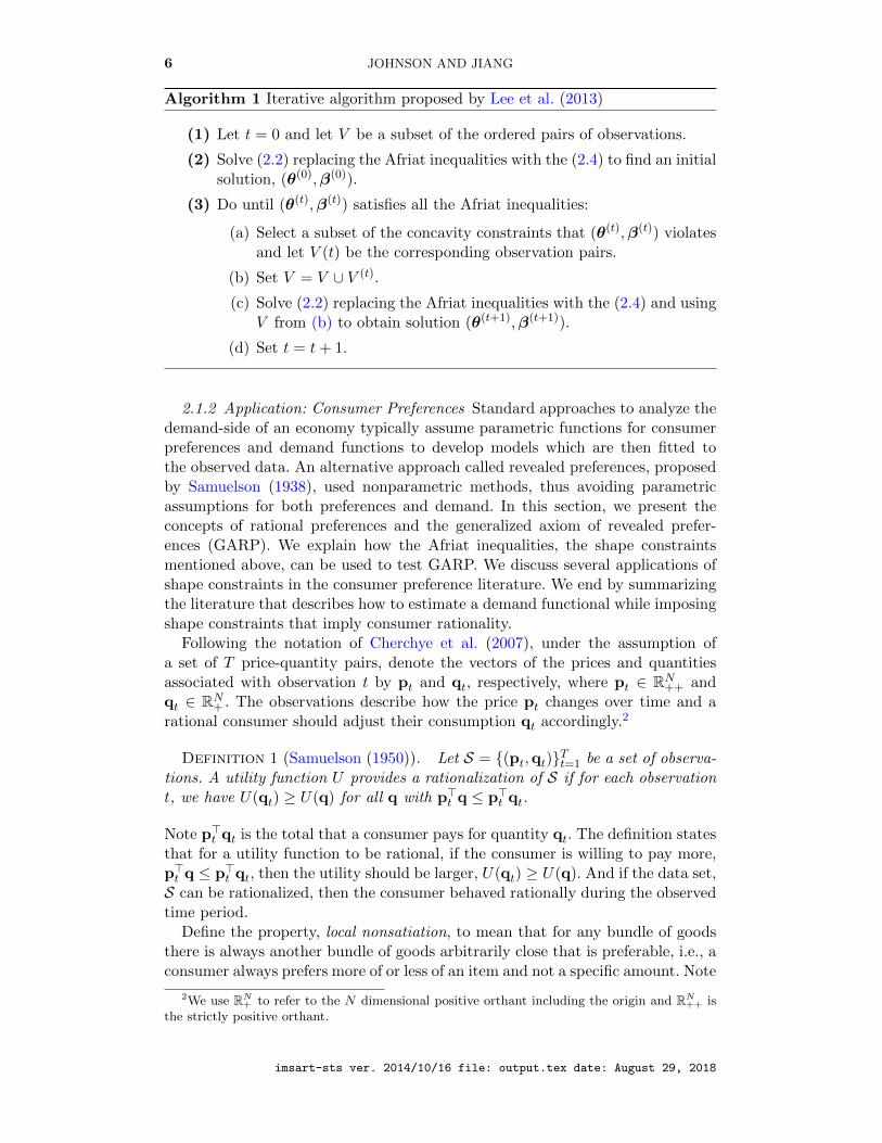
Lee et al. (2013) noted that while (2.2) is in the class of convex optimization andis thus polynomial-time solvable, the number of constraints grows quadraticallywith the size of the data set and can thus present practical challenges even for afew hundred observations. The percentage of binding constraints at the optimalsolution is only 0.5 - 1% for typical problems in economic applications. Thereforethe authors proposed an estimation procedure which initially included only theconstraints for observations that are close to one another in terms of Euclideandistance ‖Xi −Xj‖2 < C where C is prespecified parameter. Notating the set ofconstraints implied by the closeness criteria as V , the constraints are

(2.4) 〈βk,Xj −Xk〉 ≤ θj − θk ∀ k, j ∈ V,β1,β2, . . . ,βn ∈ Rd,θ ∈ Rn.

To solve a series of smaller optimization problems, Lee et al. (2013) proposed Al-gorithm 1 below, which adds back violated constraints iteratively until satisfyingthe set of all Afriat constraints. The algorithm is demonstrated for data sets ofup to 1,800 observations.

Alternatively, using a least absolute deviation loss function, which can be for-mulated as an easily solvable linear program, Luo and Lim (2016) showed thatthe estimator converges almost surely to the true function as n increases to in-finity. Mazumder et al. (2015) presented an Alternating Direction Method forMultipliers (ADMM) algorithm for solving the nonparametric LSE of a multi-variate convex regression function. Although their algorithm calculates estimatesfor data sets of 3,500 observations in less than one hour, their proposed ADMM al-gorithm has not been proven to converge for all data sets. Specifically, the ADMMalgorithm requires dividing the variables into groups and the algorithm alternatesbetween fixing all but one of the groups’ variables to their current best values andoptimizing only in terms of the selected group of variables. The ADMM algorithmhas been proven to converge for two groups of variables; however, Mazumder et al.(2015) uses three groups of variables and the converge properties of ADMM withthree groups is still an open question (Bertsekas, 1999).


6 JOHNSON AND JIANG

Algorithm 1 Iterative algorithm proposed by Lee et al. (2013)

(1) Let t = 0 and let V be a subset of the ordered pairs of observations.

(2) Solve (2.2) replacing the Afriat inequalities with the (2.4) to find an initialsolution, (θ(0),β(0)).

(3) Do until (θ(t),β(t)) satisfies all the Afriat inequalities:

(a) Select a subset of the concavity constraints that (θ(t),β(t)) violatesand let V (t) be the corresponding observation pairs.

(b) Set V = V ∪ V (t).

(c) Solve (2.2) replacing the Afriat inequalities with the (2.4) and usingV from (b) to obtain solution (θ(t+1),β(t+1)).

(d) Set t = t+ 1.

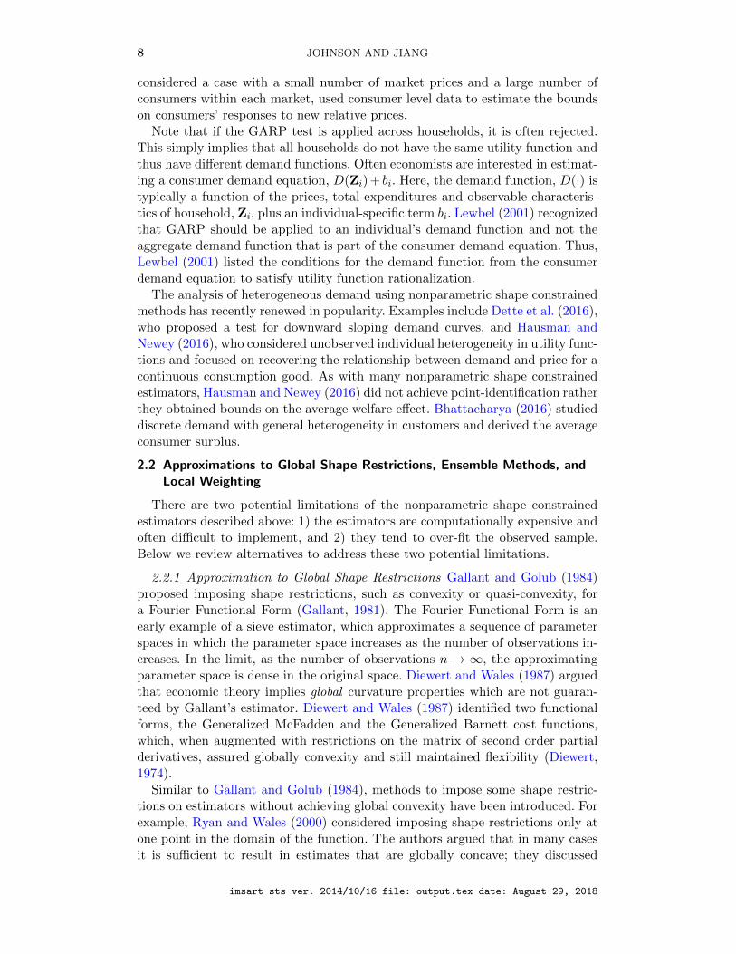
2.1.2 Application: Consumer Preferences Standard approaches to analyze thedemand-side of an economy typically assume parametric functions for consumerpreferences and demand functions to develop models which are then fitted tothe observed data. An alternative approach called revealed preferences, proposedby Samuelson (1938), used nonparametric methods, thus avoiding parametricassumptions for both preferences and demand. In this section, we present theconcepts of rational preferences and the generalized axiom of revealed prefer-ences (GARP). We explain how the Afriat inequalities, the shape constraintsmentioned above, can be used to test GARP. We discuss several applications ofshape constraints in the consumer preference literature. We end by summarizingthe literature that describes how to estimate a demand functional while imposingshape constraints that imply consumer rationality.

Following the notation of Cherchye et al. (2007), under the assumption ofa set of T price-quantity pairs, denote the vectors of the prices and quantitiesassociated with observation t by pt and qt, respectively, where pt ∈ RN++ andqt ∈ RN+ . The observations describe how the price pt changes over time and arational consumer should adjust their consumption qt accordingly.2

Definition 1 (Samuelson (1950)). Let S = (pt,qt)Tt=1 be a set of observa-tions. A utility function U provides a rationalization of S if for each observationt, we have U(qt) ≥ U(q) for all q with p>t q ≤ p>t qt.

Note p>t qt is the total that a consumer pays for quantity qt. The definition statesthat for a utility function to be rational, if the consumer is willing to pay more,p>t q ≤ p>t qt, then the utility should be larger, U(qt) ≥ U(q). And if the data set,S can be rationalized, then the consumer behaved rationally during the observedtime period.

Define the property, local nonsatiation, to mean that for any bundle of goodsthere is always another bundle of goods arbitrarily close that is preferable, i.e., aconsumer always prefers more of or less of an item and not a specific amount. Note

2We use RN+ to refer to the N dimensional positive orthant including the origin and RN

++ isthe strictly positive orthant.



strong monotonicity implies local nonsatiation but not vice versa. The revealedpreferences literature has defined a locally nonsatiated utility function that pro-vides a rationalization of the set of observations S if and only if the data satisfythe Generalized Axiom of Revealed Preferences (GARP).

In order to define GARP, we first introduce the notions of strictly directlyrevealed preferred and revealed preferred. Let S = (pt,qt)Tt=1 be a set of obser-vations. The bundle of quantities qt is strictly directly revealed preferred to q ifp>t qt > p>t q. Moreover, qt is revealed preferred to q if

p>t qt ≥ p>t qu, p>u qu ≥ p>u qv, . . . ,p

>z qz ≥ p>z q,

for some sequence (t, u, . . . , z). The set of observations S satisfies GARP if forany t and s, the bundle qt being revealed preferred to qs implies that qs is notstrictly directly revealed preferred to qt. With these definitions, we can formalizethe relationship between GARP and the existence of a utility function that canrationalize the data set S.

Theorem 2.1 (Afriat (1967); Diewert (1973); Varian (1982)). For a set S =(pt,qt)Tt=1 of observations of price-quantity pairs, the following statements areequivalent:

(1) There exists a utility function U , satisfying local nonsatiation, that providesa rationalization of S.

(2) The set S satisfies GARP, as defined above.(3) There exist U1, λ1, U2, λ2, . . . , UT , λT ∈ RN++ such that the Afriat inequali-

ties hold: for all t, r ∈ 1, 2, . . . , T,

Ur − Ut ≤ λt p>t (qr − qt).

(4) There exists a continuous monotonically increasing and concave utility func-tion U that satisfies local nonsatiation and provides a rationalization of S.

Condition (2) implies that GARP is necessary and sufficient for rationalizationof the data. While Condition (3) states that satisfying the Afriat inequalities isequivalent to satisfying GARP. Further, Condition (3) provides a test for GARP;specifically, if the Afriat inequalities are satisfied, then the set of observationsS satisfy GARP. The utility function referenced in (1) is defined as the lowerenvelope of a set of hyperplanes, specifically

U(x) = mint

Ut + λt p>t (q− qt).

Brown and Matzkin (1996) extended Afriat results to other important economicmodels; specifically, they identified restrictions on prices, incomes, and endow-ments for general equilibrium models.

GARP and the associated estimators are the workhorses for the nonparametricanalysis of demand functions. Numerous extensions have been developed, such asMatzkin (1991), who extended revealed preference analysis to nonlinear budgetsets while still imposing concave utility functions. Blundell et al. (2003) stud-ied both observations and experimental data and developed methods to detectrevealed preference violations while considering the evolution of consumer pref-erences over time modeled as an expansion path. Blundell et al. (2008), who


8 JOHNSON AND JIANG

considered a case with a small number of market prices and a large number ofconsumers within each market, used consumer level data to estimate the boundson consumers’ responses to new relative prices.

Note that if the GARP test is applied across households, it is often rejected.This simply implies that all households do not have the same utility function andthus have different demand functions. Often economists are interested in estimat-ing a consumer demand equation, D(Zi) + bi. Here, the demand function, D(·) istypically a function of the prices, total expenditures and observable characteris-tics of household, Zi, plus an individual-specific term bi. Lewbel (2001) recognizedthat GARP should be applied to an individual’s demand function and not theaggregate demand function that is part of the consumer demand equation. Thus,Lewbel (2001) listed the conditions for the demand function from the consumerdemand equation to satisfy utility function rationalization.

The analysis of heterogeneous demand using nonparametric shape constrainedmethods has recently renewed in popularity. Examples include Dette et al. (2016),who proposed a test for downward sloping demand curves, and Hausman andNewey (2016), who considered unobserved individual heterogeneity in utility func-tions and focused on recovering the relationship between demand and price for acontinuous consumption good. As with many nonparametric shape constrainedestimators, Hausman and Newey (2016) did not achieve point-identification ratherthey obtained bounds on the average welfare effect. Bhattacharya (2016) studieddiscrete demand with general heterogeneity in customers and derived the averageconsumer surplus.

2.2 Approximations to Global Shape Restrictions, Ensemble Methods, andLocal Weighting

There are two potential limitations of the nonparametric shape constrainedestimators described above: 1) the estimators are computationally expensive andoften difficult to implement, and 2) they tend to over-fit the observed sample.Below we review alternatives to address these two potential limitations.

2.2.1 Approximation to Global Shape Restrictions Gallant and Golub (1984)proposed imposing shape restrictions, such as convexity or quasi-convexity, fora Fourier Functional Form (Gallant, 1981). The Fourier Functional Form is anearly example of a sieve estimator, which approximates a sequence of parameterspaces in which the parameter space increases as the number of observations in-creases. In the limit, as the number of observations n → ∞, the approximatingparameter space is dense in the original space. Diewert and Wales (1987) arguedthat economic theory implies global curvature properties which are not guaran-teed by Gallant’s estimator. Diewert and Wales (1987) identified two functionalforms, the Generalized McFadden and the Generalized Barnett cost functions,which, when augmented with restrictions on the matrix of second order partialderivatives, assured globally convexity and still maintained flexibility (Diewert,1974).

Similar to Gallant and Golub (1984), methods to impose some shape restric-tions on estimators without achieving global convexity have been introduced. Forexample, Ryan and Wales (2000) considered imposing shape restrictions only atone point in the domain of the function. The authors argued that in many casesit is sufficient to result in estimates that are globally concave; they discussed



examples of Translog and Generalized Leontief cost functions with a single re-gressor estimated with 25 observations that produce globally concave estimates.Alternatively, considering nonparametric shape constrained estimation, Du et al.(2013) proposed imposing coordinate-wise concavity which, like Ryan and Wales(2000), can be thought of as an approximation to global concavity. However, formore complicated models, we found very little empirical evidence that imposingconcavity at a point or coordinate-wise will result in globally concave estimatesor something even close.

Other models that imposed approximations to global shape restirctions in-clude Pya and Wood (2015), who considered a generalized additive model un-der first and second order shape constraints. The estimator, which is an exten-sion of P-splines, facilitates efficient estimation of the smoothing parameters aspart of the model estimation. The authors also developed algorithms to calculatesimulation-free approximate Bayesian confidence intervals for the smooth com-ponents. Similarly, Wu and Sickles (2017) proposed a semiparametric estimatorwhich uses penalized splines and an integral transformation to impose monotonic-ity and curvature constraints. The estimator is consistent and the authors derivedthe asymptotic variance. Alternatively, Chen and Samworth (2016) considered aslightly more general model

Yi = f I(Xi) = f1(θ>1 Xi) + · · ·+ fm(θ>mXi) + c.

where the value of m ∈ N is assumed known, and Yi is the response variable andfollows an exponential family distribution. The variable c ∈ R is the interceptterm, θ1,θ2, . . . ,θm ∈ Rd are called the projection indices, and f1, f2, . . . , fm :R→ R are called the ridge functions. Chen and Samworth (2016) generalizes theclass of generalized additive models by allowing each function f to be a functionof a linear aggregation of X, specifically to the component m, θ>Xi. The benefitof this model is that shape constraints can be imposed on each of the single-dimensional functions f , making the estimator scalable and reducing the compu-tational difficulty. The drawback is that shape are only imposed coordinate-wiseand global properties are not imposed.

2.2.2 Other Shape Constrained Estimators and Ensemble Methods Hannahand Dunson (2011) proposed Multi-variate Bayesian Convex Regression (MBCR),which approximated a general convex multi-variate regression function with themaximum value of a random collection of hyperplanes. Additions, removals, andchanges of proposed hyperplanes are done through a Reversible Jump MarkovChain Monte Carlo (RJMCMC) algorithm (Green, 1995). One of MBCR’s attrac-tive features include the block nature of its parameter updating, which causes theparameter estimate autocorrelation to drop to zero in tens of iterations in mostcases. In addition, MBCR spans of all convex multi-variate functions without theneed for any acceptance-rejection samplers, scales to a few thousand observations,and relaxes the homoscedastic noise assumption.

Magnani and Boyd (2009) proposed an iterative fitting scheme to select thecovariate partitions creating K random subsets and fitted a linear model foreach subset. They constructed a convex function by taking the maximum overthese hyperplanes; the hyperplanes induced a new partition, which they used torefit the function. The series of operations repeats until reaching convergence.However, the iterative nature makes the final estimate dependent on the initial


10 JOHNSON AND JIANG

partition. Further, note the estimator is not consistent and there are cases whenthe algorithm never converges.

Alternatively, Hannah and Dunson (2013) proposed a multi-variate convexadaptive partitioning (CAP) method to estimate locally linear estimates on adap-tively selected covariate partitions. CAP uses the upper envelope of the set of locallinear estimates to construct a flexible linear hyperplane approximation to theunderlying function. The estimator is computationally feasible even for 10,000’sof observations and the authors proved its consistency, but its asymptotic rate ofconveragence is still unknown. Hannah and Dunson (2012) considered a set of en-semble methods such as bagging and smearing which could be applied to the CAPand the Magnani and Boyd (MB) estimators. Bagging subsamples the data setwith replacement taking subsample of size n repeated M times Breiman (1996).Each subsample was used to create a new estimate and then the M estimates areaveraged. Smearing adds i.i.d. mean zero noise to the observed dependent vari-able Breiman (2000). A regression model is then fitted to the new noisy data withthe observed dependent variables and the M regression estimates are averaged.Hannah and Dunson (2012) implemented smearing and bagging with both CAPand MB. The authors note the significant benefits of bagging and smearing forsmall sample sizes of 200 observations, and for their large sample sizes of 5,000observations. In application data, the MB method with either bagging or smear-ing significantly outperformed (typically by an order of magnitude on a varietyof performance criteria) CAP with no augmentations.

Yagi et al. (2018) considers the multi-variate local polynomial kernel estima-tor with shape constraints. Following their notation, define a set of m points,x1, . . . ,xm, for evaluating constraints on the local linear kernel estimator. Recallthat (Xi, Yi) : i = 1, 2, . . . , n is the set of observations. Yagi et al. (2018) definethe Shape Constrained Kernel-weighted Least Squares (SCKLS) estimator as

minimizea,b

m∑i=1

n∑j=1

(Yj − ai − (Xj − xi)> bi)

2K

(Xj − xi

h

)subject to l(xi) ≤ ψ(s)(xi |a, b) ≤ u(xi), i = 1, . . . ,m,

where a = (a1, . . . , am)> are functional estimates, b = (b>1 , . . . ,b>m)> are slope

estimates at x, K(·) denotes a product kernel, h is a vector of bandwidths3,ψ(s)(xi |a, b) is the sth derivative of the estimated function ψ, and l(xi), u(xi) arethe lower and upper bounds, respectively. Specifically, the relationship betweenψ and the variables a and b is ψ(xi) = ai and ψ(1)(xi) = bi.

Yagi et al. (2018) showed that SCKLS is consistent and its convergence ratenearly optimal (within a log factor). Unlike other nonparametric estimators,SCKLS uses local information to estimate the functional at any particular pointx, but requires bandwidth selection. Compared to other kernel based shape con-strained estimators, such as Hall and Huang (2001) and Du et al. (2013), SCKLSimposes global convexity/concavity by taking the minimum of a set of hyper-planes. A computational complexity analysis implies that SCKLS and Du et al.(2013) method should be similarly difficult to solve because both estimators aresolving quadratic objective functions relative to a convex solution spaces. How-

3See Li and Racine (2007) for more details.



ever, practically speaking, SCKLS is usually easier to solve, because the hyper-plane structure leads to a sparse constraint matrix, whereas the constraint matrixto restrict the unconstrained kernel estimator is dense making optimization moredifficult.

Semiparametric models are common in economics because standard interpre-tations apply for the linear part. Consider a function f , although unknown, pos-sesses shape properties such as homogeneity, concavity, or monotonicity. Tripathi(2000) considered the standard partially linear model, Y = X>β0 + f(Z) + ε,where Y is the response variable, (X,Z) are the covariates, β0 is a finite dimen-sional parameter of interest, and ε is an unobserved random Gaussian variable.Tripathi showed that in the class of n1/2 consistent regular estimators of the para-metric parameters β0, the concavity and monotonicity of f do not improve theefficiency of the estimate β0 in finite samples. However, homogeneity restrictionson f reduce the lower bounds for the asymptotic variance of the n1/2 consistentregular estimators of β0.

2.2.3 Application: Production Economics Microeconomic theory, which can beinterpreted as shape constraints, provides additional structure for modeling aproduction or cost function. Consider a production process that uses d differentresources to produce a single output, Y ∈ R. Call the quantity of the resourcesconsumed the inputs and use the notation, Xj ∈ Rd. Letting n instances of theproduction process, each called a production plan, lead to n pairs of input andoutput data, (Xj , Yj)nj=1. Call the set of all technologically feasible productionplans the production possibilities set and denote the set as T . Next, define theproduction function as

Yj = g0(Xj) + εj , for j = 1, . . . , n,

where εj is a random variable satisfying E(εj |Xj) = 0. Here, our primary interestis production function estimation; examples of applications to estimate the dualconcept, the cost function, using nonparametric shape constrained estimatorsinclude Beresteanu (2005) and Michaelides et al. (2015).

Microeconomic theory often implies basic assumptions, e.g. more input shouldlead to more output (at least in the input range where the production processesare observed). This particular assumption implies that the production functionincreases monotonically, specifically

if x1 ≤ x2, then g0(x1) ≤ g0(x2),

where the inequality is taken component-wise. Further, for a given output levelY , define the set of input vectors used to produce output level Y as the inputrequirement set (also referred to as the input set)

V (y) = x : (y,x) is in T .

Here, the assumption is an optimal ratio or set of ratios among the inputs existsand any deviation from the optimal ratio requires an increase in other inputs thatis more than proportional to the decrease in a particular input. Given two inputvectors x1 and x2 in V (y), then λx1 + (1 − λ)x2 is in V (y) for all 0 ≤ λ ≤ 1.Thus, V (y) is a convex set for any value y (Varian, 1992). The boundary of theinput set is referred to as the input isoquant



Isoq V (y) = x : x ∈ V (y), λx /∈ V (y), λ < 1.

The assumption of convex input sets can be strengthened. Define a productionfunction f(x) = F (g(x)). The production function is homothetic if: 1) Scalefunction F : R → R is a strictly monotone increasing function, and 2) Corefunction g : Rd → R is a homogeneous of degree 1 function which implies g(tx) =tg(x) for all t > 0. A production function that does not have this property isreferred to as non-homothetic.

The property, decreasing marginal benefit of inputs, holds for a variety of pro-duction processes. Decreasing marginal benefit of inputs implies that beyond someoutput level, Y I , the additional output that can be produced from an additionalunit of input decreases as the input level increases:

f(λx) < λf(x) for all λ ≥ 1 and f(x) ≥ yI .

There are two primary reasons for this property. First, for a particular productionprocess certain inputs are well-matched or are the best inputs for that process.Scarcity of inputs is the notion that as the scale of production increases, lessideal inputs are used, and so less output per unit of input is achieved. Second,as a production process increases, the related activities are harder to organizeor control. Economists call this the span of control. A production function withconvex input sets that satisfies decreasing marginal benefit of inputs over theentire input space (i.e., yI = 0) is globally concave (Varian, 1984).

For multi-product production, Mundlak (1963) defined a multi-product outputvector y = (y1, y2, . . . , yq)

> ∈ Rq+. For a given input vector x, define the set ofoutput vectors that can be produced as the producible output set :

L(x) = y : (y,x) is in T .

Mundlak (1963) argued that the producible output set L(x) should also be con-vex. This leads naturally to an implicit multi-input/multi-output production func-tion, also called the transformation function, defined as:

f(y,x) = 0.

Under the assumption that the input requirement and the producible output setsare convex and that the scaling relationship between inputs and output increasesmonotonically with the decreasing marginal product, Chambers (1988) shows themulti-input/multi-output production technology T is globally convex. Further,Chambers (1988) defined the the properties a multi-input/multi-output produc-tion technology should satisfy and Kuosmanen and Johnson (2017) provided anonparametric shape constrained estimator for this technology.

Historically, much of the literature on production functions concerned endo-geneity. For example, management would determine input levels with knowl-edge of its firm-specific characteristics and potentially partial knowledge of ran-dom shocks. In the production model, the assumption E(ε |X) is violated, lead-ing to biased and inconsistent estimates. A variety of solutions have been pro-posed when the production function is estimated parametrically (Griliches andMairesse, 1995; Ackerberg et al., 2015). Florens et al. (2018) considered estimat-ing a nonparametric shape constrained function using a kernel–based approach



with Landweber–Fridman regularization techniques using instrumental variablesto address endogeneity. Research which combines shape constraints with treat-ment of endogenous variables when estimating production functions is a promis-ing development.

2.3 Single Index Models and Alternative Assumptions to Global Convexity

The desire to maintain convex (linear) input sets while relaxing the concavityassumption for the relationship between the dependent variable and the regres-sors leads naturally to single index models. Consider the following single indexregression model:

Y = m0(θ>0 X) + ε.

Here, Xi ∈ Rd is an observed vector of predictors where d ≥ 1, ε1, ε2, . . . , εnsatisfy E(εi |Xi) = 0, θ0 are the parameters of a linear function to project X toa single dimension, and m0 : Rd → R is an unknown link function. The singleindex model averts the curse of dimensionality typical of nonparametric regres-sion functions with a vector of predictors. This specification states that the linkfunction depends on X only through a one dimensional projection θ>0 X. Shaperestrictions are often placed on the link function m0. Balabdaoui et al. (2016),who studied this model under a monotonicity constraint on m0, proved consis-tency of the least squares estimator and Balabdaoui et al. (2017) proved thatthe least squares estimator achieves the n−1/2 rate of convergence. Kuchibhotlaet al. (2017) considered both a Lipschitz constrained least squares estimator andthe penalized least squares estimator and found similar results for consistencyand rate of convergence. The single index model adds structure to the estimator,which can be useful particularly when the data are limited. However, assuminglinear substitution between inputs or goods, θ>0 X, can be overly restrictive formany production or utility models.

2.3.1 Application: Production Functions Continued Convex input sets are typ-ically a maintained assumption in production economics, but alternative assump-tions are available for the scaling law (or the relationship between output andexpanding input levels). While decreasing marginal product is a common charac-teristic for large firms, economists often assume an increase in marginal productfor production at a small scale, i.e. increasing returns to scale. Thus, a propor-tional increase in inputs leads to a more than proportional increase in output

f(λx) > λf(x) for all λ ≥ 1.

The primary reasons for the increasing returns to scale are the benefit of special-ization and the reduction in change-over time when switching between compo-nents of the production process.

Frisch (1964) proposed the Regular Ultra Passum (RUP) production law. Thelaw outlines when a firm is operating at a small scale size it can achieve significantincreases in output for incremental increase in input through specialization andlearning. In contrast, as the scale size becomes larger, a firm tends to face scarcityof ideal production inputs and challenges related to increasing span of control,thus the marginal benefits of additional inputs decrease. Based on these concepts,



define the elasticity of scale,4 ε(x), relative to a production function f(x):

(2.5) ε(x) =

d∑k=1

∂f(x)

∂xk

xkf(x)

,

and define the RUP law as follows.

Definition 2 (Førsund and Hjalmarsson (2004)). A production functionf(x) obeys the Regular Ultra Passum Law if ∂ε(x)/∂xk < 0, and there existinput vectors xa and xb where xb ≥ xa component-wise such that ε(xa) > 1while ε(xb) < 1.5

While the RUP law is often not referred to by name, most introductory mi-croeconomic textbooks introduce the concept (Perloff, 2018). Further, researcherscommonly assume that along a given ray, there exists only a single inflectionpoint; however, neither Førsund and Hjalmarsson (2004) nor Frisch (1964) defi-nition rules out this possibility. To make this concept rigorous, Yagi et al. (2018)defined an S-shape function.

Definition 3 (Yagi et al. (2018)). For any vector v ∈ Rd+ and the associatedray from the origin in input space αv with α > 0, a production function f : Rd →R is S-shaped if there exists an x∗ such that ∇2

vf(αv) > 0 for αv < x∗, and∇2

vf(αv) < 0 for αv > x∗, where ∇2vf is the directional second derivative of f

along v. This implies that for any ray from the origin in the direction v, thereexists a single inflection point x∗ that ∇2

vf(x∗) = 0.

In defining an S-shape production function, Yagi et al. (2018) derived the rela-tionship to the long standing concept of the RUP law. Specifically, if a productionfunction f : Rd → R is twice-differentiable, monotonically increasing, satisfies theRUP law, and has a single inflection point, then f is S-shaped.

Yagi et al. (2018) proposed an estimation algorithm for a non-homothetic pro-duction function satisfying both the S-shape definition and input convexity with-out any further structural assumptions. The algorithm has two steps: (1) Estimateinput isoquants for a set of output levels, and (2) estimate S-shape functions ona set of rays from the origin. A CNLS-based estimator is used for isoquant es-timation and a SCKLS-based estimators for the S-shape estimation. While thisestimator has a similar flavor as the single index model, relaxing the parameterstructure for aggregating the vector of inputs necessitates a two step procedure.In the non-homothetic case, the performance of the estimator can be improvedby iterating between the two-steps. However, if the production function is homo-thetic, the input isoquant can be estimated for just a single output level as inHwangbo et al. (2015).

4This variable, formerly referred to as the passum coefficient in the seminal work of Frisch(1964), is now commonly referred to as the elasticity of scale.

5Note that this definition of the RUP law is slightly adapted from Førsund and Hjalmarsson(2004) for clarity. Førsund and Hjalmarsson (2004) definition generalizes Frisch (1964) originaldefinition by not requiring the passum coefficient to go below 0 implying congestion. This gen-eralization also allows for a monotonically increasing production function. Further, a concaveproduction function nests within this definition.



In the future, the availability of shape constrained nonparametric estimationtechniques could allow economists to develop alternative theories of productionand validate them empirically.

3. SEQUENTIAL DECISION MAKING

Making sequential decisions under uncertainty, which has been studied ex-tensively in both economics and operations research, is formalized under dy-namic programming, optimal control, Markov decision processes, and other topics(Stokey et al., 1989; Kamien and Schwartz, 1981; Puterman, 1994). The typicalsetting consists of a decision-maker who alternates between making decisions andobserving new information, to inform future decisions:

choose decision observe information choose next decision · · ·

In a sequential setting where stochastic information is revealed over time, thedecision maker needs to find the optimal policy that prescribes a decision for everypossible “state-of-the-world” i.e., every outcome of the stochastic informationprocess. The following example, illustrates the well-known problem of multi-stageinventory management (Clark and Scarf, 1960; Scarf, 1960; Porteus, 2002).

Consider a firm managing its inventory control policy over a finite horizon ofT periods. At time period t, the decision maker observes the current inventorystate st and places an order for xt additional units. Between time t and time t+1,a random demand Dt+1, independent of the past, is realized. The cost functionfor period t is given by

(3.1) ct(st, xt) = cxt + E[h(st + xt −Dt+1)

+ + b(Dt+1 − st − xt)+],

where c is the ordering cost, h is the holding cost, and b is the backlogging cost(i.e., cost per unit of unsatisfied demand). The inventory position at t + 1 isgiven by st+1 = st +xt−Dt+1, where st < 0 represents unsatisfied or backloggeddemand. The decision maker needs to determine the optimal inventory orderingpolicy π∗t (a function mapping inventory states st to order quantities xt) thatminimizes the expected cumulative cost E

[∑T−1t=0 ct(st, πt(st))

].

At every period t, the decision maker needs to determine an order quantityxt for each possible inventory state st (a scalar quantity). This model is knownas a finite-horizon Markov decision process (MDP) (Puterman, 1994). If st takeson a finite number of values and the expected value is easy to compute (e.g.,in the case where order quantities are integer-valued and demands are integer-valued and bounded), then the optimal decision in stage t, state s, denoted π∗t (st),can be computed by simply enumerating the inventory states and then applyinga standard dynamic programming method (Bertsekas, 2012; Puterman, 1994).This amounts to solving a series of recursive equations to compute the so-calledoptimal value functions. Let VT (s) ≡ 0 and for each t < T , define the optimalvalue function

(3.2) Vt(st) = minxt

ct(st, xt) + E[Vt+1(st + xt −Dt+1)]

.

Here, the optimal decision in state st at time t is an xt that achieves the minimumof the right-hand-side of (3.2). Thus, solving for the optimal policy π∗t for each t



under the dynamic programming framework depends on the decision maker’s abil-ity to compute the value functions, Vt. Although the recursive equations may seemsimple, realistic instances of the inventory control problem can quickly becomeintractable for the enumeration-based dynamic programming method discussedabove. For example,

• Consider the case of a multi-product inventory system, as described in Evans(1967) or Aviv and Federgruen (2001). In this setting, the decision makerneeds to track the inventory states for all products; thus, st becomes multi-dimensional. Even if the number of inventory states per product is enumer-able, the number of states across all products grows exponentially with thenumber of products; this is an example of the “curse of dimensionality.”• The assumption that Dt+1 is independent of the past is called stage-wise

independence (Pereira and Pinto, 1991; Shapiro, 2011). In practical ap-plications, the distribution of the demand could depend on factors suchas weather, previous demands, or market conditions represented by it.Consequently, the optimal policy depends on both st and it, and is writ-ten as π∗t (st, it). Computational difficulties easily arise when it is multi-dimensional, again due to the curse of dimensionality.• An unknown distribution for Dt+1 implies the inability to compute the ex-

pectation in (3.1). This limitation, which prevents the application of stan-dard dynamic programming techniques, forces the decision maker to usesample-based methods, usually historical data or a simulator (generativemodel).

Approximate dynamic programming (ADP) and reinforcement learning (RL)refer to a set of methodologies and algorithms for approximately solving com-plex sequential decision problems when the state space is large and/or partsof the system are unknown (Bertsekas and Tsitsiklis, 1996; Sutton and Barto,1998; Bertsekas, 2012; Powell, 2011). For general large-scale problems, unstruc-tured approximations including value iteration with linear approximations (i.e.,using basis functions) (De Farias and Van Roy, 2000; Tsitsiklis and Roy, 1996;Tsitsiklis and Van Roy, 1999; Geramifard et al., 2013), approximate linear pro-gramming (De Farias and Van Roy, 2003; De Farias and Van Roy, 2004; Desaiet al., 2012a), and nonparametric methods are used (Ormoneit and Sen, 2002;Bhat et al., 2012). Recently, RL with deep neural networks has become pop-ular (Mnih et al., 2015; Silver et al., 2016). Structured approximations can beincorporated when properties can be identified a priori.

The next section reviews the uses of shape constraints to enforce structurein the approximations used in ADP and RL. The primary focus is on convexityof the value function, a particularly well-studied shape constraint in sequentialdecision problems (Pereira and Pinto, 1991; Godfrey and Powell, 2001; Philpottand Guan, 2008; Nascimento and Powell, 2009, 2010), and the secondary focusis monotonicity (Papadaki and Powell, 2002; Jiang and Powell, 2015), which isuseful when convexity is not available. We conclude with a brief review of howpolicy structure can be exploited (Kunnumkal and Topaloglu, 2008b; Huh andRusmevichientong, 2009; Zhang et al., 2017). The notation we use will largelyfollow the standards of the literature.



3.1 Convexity of the Value Function

In many problems, the value function Vt is convex in the state variable, or, atleast in certain dimensions of the state variable, for each t. One benefit of theproperty of convexity is the potential for algorithms to exploit this structure.Below, we survey several widely used and powerful methodologies.

3.1.1 Stochastic Decomposition We begin with the two-stage linear programwith recourse (Birge and Louveaux, 2011). The recourse decisions are made in thesecond (and final stage) after uncertainties have been realized. The interpretationis that the “mistakes” made by the first-stage decision (e.g., inventory shortage)can be corrected in the second stage. Let X be a convex, polyhedral set. Usingthe notation of Higle and Sen (1991), formulate the problem as

minimizex

f(x) = c>x+ Eh(x, ω)

subject to x ∈ X ,

where h(x, ω) is the optimal objective function value of the second-stage problem

minimizey

g>y

subject to Wy = ω − Txy ≥ 0.

Here, c is a cost vector and x is the first-stage decision, which must be chosenbefore the realization of a random variable ω. The second-stage recourse costs aregiven by g and the associated decision is y. The recourse matrix is W and ω−Txis discrepancy that is accounted for in the second stage by y. Assume that valuefunction h is finite. To illustrate the formulation, in a production problem, x mayrepresent raw material order quantities from a supplier (at cost c) to produce Txunits of a product; ω is the realized demand and ω− Tx is a shortage; and y arethe raw material order quantities from an emergency supplier (at costs g), whichcan produce Wy units of the product.

The stochastic decomposition (SD) algorithm proposed by Higle and Sen (1991)exploits the convexity and piecewise-linearity of h(x, ω) by combining ideas fromBender’s decomposition and stochastic approximation (Kushner and Yin, 2003).The algorithm constructs a necessarily convex approximation of the objectivefunction f by defining it as the maximum of iteratively computed hyperplanes.The steps of the stochastic decomposition method are summarized below.

(1) Subproblem. Given xk on iteration k, compute the solution to the second-stage problem for a single sample ωk generated from the distribution of ωby using a dual formulation, with dual variables π

h(xk, ωk) = maxπ

π>(ωk − Txk) |W>π ≤ g

.

(2) Compute Cut. Using all subproblem solutions generated until iteration k,estimate the support of f(x) via an affine function αkt + (βkt + c)x. Thisaffine function is called a cut. See (Higle and Sen, 1991, Section 2.2) for thedetails.



(3) Update Old Cuts. Reduce the influence of the old cuts generated in iterationst < k via the updates

αkt = (k − 1)αk−1t /k and βkt = (k − 1)βk−1t /k.

(4) Update Convex Approximation. Compute the piecewise-linear and convexapproximation of the objective function f(x) as a maximum of affine func-tions:

fk(x) = maxt≤k

αkt + (βkt + c)x

The iterate xk+1 is a solution to an approximate first-stage problem givenby maxx∈X fk(x).

Theorem 3.1 (Higle and Sen (1991)). There exists a subsequence of xkgenerated by SD, such that every accumulation point of the subsequence is anoptimal solution, with probability one.

The formal statement of the SD algorithm also uses the concept of an incumbentsolution, which roughly speaking, is an iterate which achieves a low objectivevalue and is revisited by the algorithm. Such an implementation improves themethod’s empirical performance and does not affect the convergence guarantee.However, despite asymptotic guarantees, stopping rules are critical for practicalimplementations (see, e.g., Higle and Sen (1996); Mak et al. (1999)). The originalSD algorithm was designed only for two-stage problems, but more recently, Senand Zhou (2014) proposed a regularized, multi-stage extension.

3.1.2 Stochastic Dual Dynamic Programming The stochastic dual dynamic pro-gramming (SDDP) algorithm was first proposed by Pereira and Pinto (1991).SDDP was proposed before SD, but both are based on the idea of iterativelygenerating cuts to approximate a piecewise-linear convex value function. The dif-ference is that SDDP does not use stochastic approximation (i.e., the phase-outstep), but requires the subproblems to be solved for every scenario in each it-eration. SDDP is more general in the sense that it was directly proposed formultistage problems.

We introduce the multistage stochastic linear programming model using thenotation of Philpott and Guan (2008), while noting that it is a direct extensionof the two-stage model discussed in the previous section. Let Ωt be a finite set ofrandom outcomes for state t, where outcome ωti has probability pti. The randomvariables ωt ∈ Ωt are independent across time (termed stagewise independence).Let QT+1 ≡ 0 and define Qt(xt−1) =

∑i ptiQt(xt−1, ωti), where

(3.3)

Qt(xt−1, ωti) = minxt

ctxt +Qt+1(xt)

subject to At xt = ωt −Bt−1xt−1xt ≥ 0,

and write the first-stage problem as

Q1 = minxt

c1x1 +Q2(x1)

subject to A1 x1 = b1

x1 ≥ 0.



Once again, the value functions Qt(x) are piecewise-linear convex (Pereira andPinto, 1991), so the approximation used in SDDP is a maximum of hyperplanes.Let Qkt be the approximation of Qt at iteration k and suppose QkT+1 = QT+1 forall k. The main steps of iteration k of the algorithm are as follows.

(1) Forward Pass. For each time period t = 1, 2, . . . , T , select a trial decisionxkt . There are a variety of ways to do this, but the original proposal fromPereira and Pinto (1991) is to simulate one sample of the decisions generatedby the current policy, i.e., the one induced by solving (3.3) where Qt+1 isreplaced with the current approximate value function Qk−1t+1 .

(2) Backward Pass. SDDP now moves backward, starting from t = T . At thetrial decision xkt , loop through all possible outcomes of the random variableωt and for each outcome ωti, solve the problem (3.3) with Qkt+1 replacingQt+1 and ωti replacing ωt. Compute a cut and use it to update the approxi-mation for time t, resulting in Qkt (which is used in the subproblem solved inat t−1). Note that the convexity of Qt is again exploited by approximatingit as the maximum of a series of affine cuts.

The convergence of the SDDP algorithm has been studied by Linowsky andPhilpott (2005) and further generalized by Philpott and Guan (2008). Note thatthe improvement of the convergence result here compared to the one for SD isbecause all scenarios are being considered when computing the cuts.

Theorem 3.2 (Philpott and Guan (2008)). Under some technical assump-tions on the forward pass, the SDDP algorithm converges to an optimal solutionof the first-stage problem in a finite number of iterations.

Two algorithms closely related to SDDP are the cutting plane and partial sam-pling algorithm of Chen and Powell (1999) and the abridged nested decompositionalgorithm of Donohue and Birge (2006). Notably, the convergence of both meth-ods follows from Philpott and Guan (2008). The stagewise independence assump-tion of the random process was relaxed in Lohndorf et al. (2013) and Asamovand Powell (2018). Asamov and Powell (2018) also proposed a regularized versionof SDDP to improve performance. Extensions of SDDP for risk-averse problemswere explored in Philpott and de Matos (2012), Shapiro et al. (2013), and Philpottet al. (2013). All of these methods enforce a convex “shape constraint” on thevalue function approximation via a piecewise-linear function.

Example (Hydrothermal Planning). Hydrothermal operations planning hasa long history in the operations research literature (Pereira and Pinto, 1991;Pritchard et al., 2005; Philpott and de Matos, 2012; Shapiro et al., 2013; Maceiraet al., 2015). The objective is to find an operational strategy that satisfies energydemand at every location in the system while achieving minimal expected cost.Below, we summarize the major features.

• The overall system contains a set of reservoirs whose storage levels aretracked by the state variable. From period to period, the reservoir is subjectedto stochastic inflows and potential losses due to evaporation.• Water stored in the reservoirs can be used for (free) energy production.

Thermal generators used to complement the hydroelectric production are



expensive to operate, i.e., each generator has an associated generation costfunction.• Energy can be interchanged between two locations via transmission lines.

This feature emphasizes the influence of the underlying network structure.

Discretization and standard dynamic programming cannot be used, because of theincreased number of states as the number of reservoirs increases. Instead, SDDPis used to provide approximations of the optimal policy for problems ranging insize from 22 reservoirs (Pereira and Pinto, 1991) to 69 reservoirs (Shapiro et al.,2013).

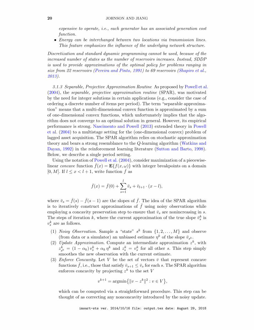
3.1.3 Separable, Projective Approximation Routine As proposed by Powell et al.(2004), the separable, projective approximation routine (SPAR), was motivatedby the need for integer solutions in certain applications (e.g., consider the case ofordering a discrete number of items per period). The term “separable approxima-tion” means that a multi-dimensional convex function is approximated by a sumof one-dimensional convex functions, which unfortunately implies that the algo-rithm does not converge to an optimal solution in general. However, its empiricalperformance is strong. Nascimento and Powell (2013) extended theory in Powellet al. (2004) to a multistage setting for the (one-dimensional convex) problem oflagged asset acquisition. The SPAR algorithm relies on stochastic approximationtheory and bears a strong resemblance to the Q-learning algorithm (Watkins andDayan, 1992) in the reinforcement learning literature (Sutton and Barto, 1998).Below, we describe a single period setting.

Using the notation of Powell et al. (2004), consider maximization of a piecewise-linear concave function f(x) = Ef(x, ω) with integer breakpoints on a domain[0,M ]. If l ≤ x < l + 1, write function f as

f(x) = f(0) +

l∑s=1

vs + vl+1 · (x− l),

where vs = f(s)− f(s− 1) are the slopes of f . The idea of the SPAR algorithmis to iteratively construct approximations of f using noisy observations whileemploying a concavity preservation step to ensure that vs are nonincreasing in s.The steps of iteration k, where the current approximation of the true slope vks isvks are as follows.

(1) Noisy Observation. Sample a “state” sk from 1, 2, . . . ,M and observe(from data or a simulator) an unbiased estimate ηk of the slope vsk .

(2) Update Approximation. Compute an intermediate approximation zk, withzksk

= (1 − αk) vks + αk η

k and zks = vks for all other s. This step simplysmoothes the new observation with the current estimate.

(3) Enforce Concavity. Let V be the set of vectors v that represent concavefunctions f , i.e., those that satisfy vs+1 ≤ vs for each s. The SPAR algorithmenforces concavity by projecting zk to the set V

vk+1 = argmin‖v − zk‖2 : v ∈ V

,

which can be computed via a straightforward procedure. This step can bethought of as correcting any nonconcavity introduced by the noisy update.



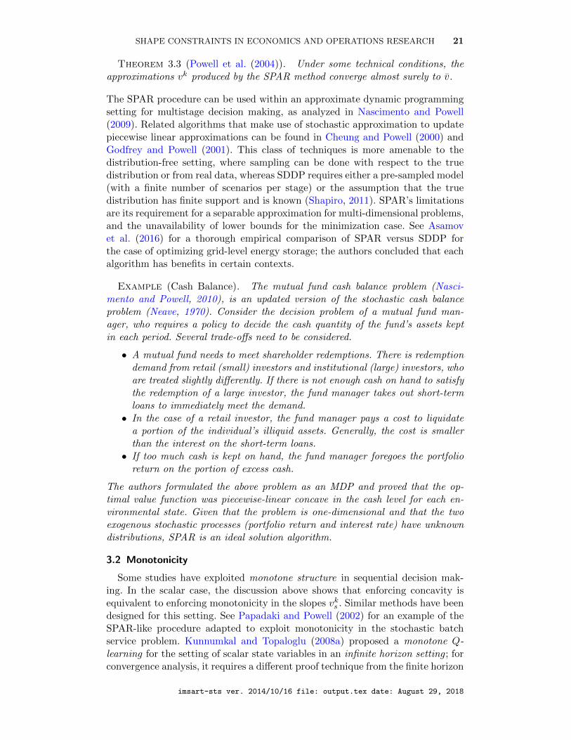
Theorem 3.3 (Powell et al. (2004)). Under some technical conditions, theapproximations vk produced by the SPAR method converge almost surely to v.

The SPAR procedure can be used within an approximate dynamic programmingsetting for multistage decision making, as analyzed in Nascimento and Powell(2009). Related algorithms that make use of stochastic approximation to updatepiecewise linear approximations can be found in Cheung and Powell (2000) andGodfrey and Powell (2001). This class of techniques is more amenable to thedistribution-free setting, where sampling can be done with respect to the truedistribution or from real data, whereas SDDP requires either a pre-sampled model(with a finite number of scenarios per stage) or the assumption that the truedistribution has finite support and is known (Shapiro, 2011). SPAR’s limitationsare its requirement for a separable approximation for multi-dimensional problems,and the unavailability of lower bounds for the minimization case. See Asamovet al. (2016) for a thorough empirical comparison of SPAR versus SDDP forthe case of optimizing grid-level energy storage; the authors concluded that eachalgorithm has benefits in certain contexts.

Example (Cash Balance). The mutual fund cash balance problem (Nasci-mento and Powell, 2010), is an updated version of the stochastic cash balanceproblem (Neave, 1970). Consider the decision problem of a mutual fund man-ager, who requires a policy to decide the cash quantity of the fund’s assets keptin each period. Several trade-offs need to be considered.

• A mutual fund needs to meet shareholder redemptions. There is redemptiondemand from retail (small) investors and institutional (large) investors, whoare treated slightly differently. If there is not enough cash on hand to satisfythe redemption of a large investor, the fund manager takes out short-termloans to immediately meet the demand.• In the case of a retail investor, the fund manager pays a cost to liquidate

a portion of the individual’s illiquid assets. Generally, the cost is smallerthan the interest on the short-term loans.• If too much cash is kept on hand, the fund manager foregoes the portfolio

return on the portion of excess cash.

The authors formulated the above problem as an MDP and proved that the op-timal value function was piecewise-linear concave in the cash level for each en-vironmental state. Given that the problem is one-dimensional and that the twoexogenous stochastic processes (portfolio return and interest rate) have unknowndistributions, SPAR is an ideal solution algorithm.

3.2 Monotonicity

Some studies have exploited monotone structure in sequential decision mak-ing. In the scalar case, the discussion above shows that enforcing concavity isequivalent to enforcing monotonicity in the slopes vks . Similar methods have beendesigned for this setting. See Papadaki and Powell (2002) for an example of theSPAR-like procedure adapted to exploit monotonicity in the stochastic batchservice problem. Kunnumkal and Topaloglu (2008a) proposed a monotone Q-learning for the setting of scalar state variables in an infinite horizon setting ; forconvergence analysis, it requires a different proof technique from the finite horizon



setting of Nascimento and Powell (2013). However, for a multi-dimensional state,Kunnumkal and Topaloglu (2008a) suggest arbitrarily selecting a dimension inwhich monotonicity is enforced.

Jiang and Powell (2015) proposed monotone-ADP, extending previous work tothe multi-dimensional state space setting. More generally, the algorithm applieswhen monotonicity is preserved over partially ordered states. Consider a dynamicprogramming setting similar to (3.2), where the value functions Vt(s) satisfy

Vt(s) ≤ Vt(s′) for all s s′,

where is a partial order over the state space. Monotone-ADP is useful in thesetting of s = (x1, x2, . . . , xd) and s′ = (x′1, x

′2, . . . , x

′d) with monotonicity in the

value function whenever xi ≤ x′i for all i. The steps of the algorithm are analogousto those of SPAR, except in a multistage setting. For example, in iteration k, thereis a state skt , an updated value zkt , and a current value function approximationV kt . Here, we focus on a new operator ΠM , which depends on skt , z

kt , and V k

t ,where there is an arbitrary state s and the output is the updated value of states after accounting for the new observation at skt and the monotone structure.Define it as

ΠM

(skt , z

kt , V

kt

)(s) =

zkt if s = skt ,

zkt ∨ V kt (s) if skt s, s 6= skt ,

zkt ∧ V kt (s) if skt s, s 6= skt ,

Vt(s) otherwise,

where a ∨ b = max(a, b) and a ∧ b = min(a, b). The first condition says that thevalue of skt is updated to zkt regardless of the other values, which is a departurefrom SPAR. The second condition says that if s is greater than skt , then its valueshould be the maximum of zkt and V k

t under the monotonicity condition. Thethird condition similarly covers the case of s less than skt . The fourth conditionleaves the “incomparable” states unchanged, because there is only a partial orderover the states.

Theorem 3.4 (Jiang and Powell (2015)). Under some technical assumptions,the approximation V k

t (s) generated by monotone-ADP converges to the valuefunction Vt(s) almost surely for each stage t and state s.

Since the theoretical basis of the monotone-ADP algorithm is stochastic ap-proximation, this theorem emphasizes that the monotone shape constraint doesnot affect its convergence properties.

Example (Optimal Stopping). Perhaps the most fundamental problem classin sequential decision making concerns the question of optimal stopping or optimalreplacement (Pierskalla and Voelker, 1976; Rust, 1987; Tsitsiklis and Van Roy,1999; Kurt and Maillart, 2009; Kurt and Kharoufeh, 2010; Desai et al., 2012b).The trade-off in the case of optimal stopping is whether the decision maker shouldaccept the reward now (e.g., sell a house), or wait until a future period (e.g., waitfor a higher offer). Similarly, optimal replacement problems model the trade-offbetween the cost of replacement now versus the possibility of failure in the future.



Although such problems do not feature convex value functions, they often con-tain many exogenous information states, which impose significant computationalchallenges. Fortunately, monotonicity can sometimes hold. For example, Kurtand Maillart (2009) and Kurt and Kharoufeh (2010) showed that under certainconditions, the value function of an optimal replacement model was nondecreasingin both the system state (health of the system to be replaced) and the environmen-tal state, i.e. an opportunity for monotone shape constraints to be utilized wasprovided. Jiang and Powell (2015), who applied the monotone-ADP algorithmto problems of this type, showed significant empirical improvements when mono-tonicity was enforced.

3.3 Policy Structure

The final goal of sequential decision making problems is to discover the opti-mal policy. Computing the optimal value function is one approach, but it is alsopossible to directly search for the optimal policy π∗t (s). Consider the well-knownpolicy gradient methods of reinforcement learning (Sutton et al., 2000). In op-erations research, the structure of optimal policies are often known a priori formany foundational models. Below, we give an example of using shape constraintsin the policy space.

It is well-known that the optimal policy to the inventory control applicationdiscussed above is of basestock form (for example see Porteus (2002)), meaningthat optimal basestock levels rt exist such that if the current inventory levelis st, then it is optimal to place an order for xt = [rt − st]+ units of inventory.In other words, if st is below rt, the decision maker orders up to rt, and if st isabove rt, it does not order.

Kunnumkal and Topaloglu (2008b) proposed an algorithm that directly searcheswithin the class of all basestock policies, in effect imposing a “basestock shapeconstraint” throughout the search. The authors considered a stochastic approxi-mation approach, where rkt denotes the estimated basestock levels at iterationk. The two steps are as follows.

(1) Demand Observations. Observe either from data or within a simulated set-ting, a trajectory of demand realizations

Dk = (Dk1 , D

k2 , . . . , D

kT ).

Note that demand is exogenous to the inventory system.(2) Basestock Update. Using the current basestock levels rkt and the demand

observations Dk, compute an estimated basestock adjustment ∆kt to im-

prove the performance of the basestock policy. The update is given by

rk+1t = rkt − αk∆k

t

for some stepsize or learning-rate αk.

Because no value function approximation is stored, the calculation of ∆kt is non-

trivial and requires a novel recursive computation derived from the Bellman equa-tion (Kunnumkal and Topaloglu, 2008b, Section 3).

Theorem 3.5 (Kunnumkal and Topaloglu (2008b)). Under various technicalconditions, the sequence of basestock policies generated by the method above isasymptotically optimal: rkt → rt almost surely for each t.



A basestock shape constraint was also used in the online convex optimizationapproach of Huh and Rusmevichientong (2009). A related paper by Zhang et al.(2017), used the basestock shape constraint in a perishable inventory setting todiscover good, but not necessarily optimal, policies.

4. DISCUSSION

The economics and operations research communities continue to propose, test,and debate new applications of shape constrained estimation. This paper brieflysurveys several significant applications of shape constraints, including revealedpreferences, production economics, and several operational problems that involvesequential decision making. To our knowledge, this survey is the first to reviewthe operations research literature on shape constraints.

Shape constraints, including monotonicity, convexity/concavity, and S-shapes,have attracted research from both practical and theoretical perspectives. The ad-ditional structure provided by imposing shape constraints allows for estimationwith smaller samples, and in the case of sequential decision making applications,structured versions of approximate dynamic programming algorithms enablespractitioners to address large-scale problems. We expect that new methodolo-gies will be developed to address other important problem structures, which willin turn facilitate the growth of the fields of economics and operations research.

ACKNOWLEDGEMENTS

We are grateful to Bodhisattva Sen and Richard Samworth for inviting us towrite this paper. Andrew thanks Osaka University for its financial support. Anymistakes are our own. The views expressed herein are those of the authors.



REFERENCES

Ackerberg, D. A., K. Caves, and G. Frazer (2015). Identification properties of recent productionfunction estimators. Econometrica 83 (6), 2411–2451.

Afriat, S. N. (1967). The construction of utility functions from expenditure data. Internationaleconomic review 8 (1), 67–77.

Afriat, S. N. (1972). Efficiency estimation of production functions. International EconomicReview 13 (3), 568–598.

Aıt-Sahalia, Y. and J. Duarte (2003). Nonparametric option pricing under shape restrictions.Journal of Econometrics 116 (1), 9–47.

Alizadeh, F. (2006). Semidefinite and second-order cone programming and their application toshape-constrained regression and density estimation. In Models, Methods, and Applicationsfor Innovative Decision Making, pp. 37–65.

Allon, G., M. Beenstock, S. Hackman, U. Passy, and A. Shapiro (2007). Nonparametric estima-tion of concave production technologies by entropic methods. Journal of Applied Economet-rics 22 (4), 795–816.

Asamov, T. and W. B. Powell (2018). Regularized decomposition of high-dimensional multistagestochastic programs with Markov uncertainty. SIAM Journal on Optimization 28 (1), 575–595.

Asamov, T., D. F. Salas, and W. B. Powell (2016). SDDP vs. ADP: The effect of dimen-sionality in multistage stochastic optimization for grid level energy storage. arXiv preprintarXiv:1605.01521.

Aviv, Y. and A. Federgruen (2001). Capacitated multi-item inventory systems with randomand seasonally fluctuating demands: implications for postponement strategies. Managementscience 47 (4), 512–531.

Balabdaoui, F., C. Durot, and H. Jankowski (2016). Least squares estimation in the monotonesingle index model. arXiv preprint arXiv:1610.06026.

Balabdaoui, F., P. Groeneboom, and K. Hendrickx (2017). Score estimation in the monotonesingle index model. arXiv preprint arXiv:1712.05593.

Banker, R. D. and A. Maindiratta (1992). Maximum likelihood estimation of monotone andconcave production frontiers. Journal of Productivity Analysis 3 (4), 401–415.

Barlow, R. E., D. J. Bartholomew, J. M. Bremner, and H. D. Brunk (1972). Statistical InferenceUnder Order Restrictions; The Theory and Application of Isotonic Regression. Wiley, NewYork.

Beresteanu, A. (2005). Nonparametric analysis of cost complementarities in the telecommuni-cations industry. RAND Journal of Economics 36 (4), 870–889.

Beresteanu, A. et al. (2007). Nonparametric estimation of regression functions under restrictionson partial derivatives. Preprint. http://www.econ.duke.edu/ arie/shape.pdf.

Bertsekas, D. P. (1999). Nonlinear programming. Athena scientific Belmont.Bertsekas, D. P. (2012). Dynamic programming and optimal control, Vol. II: Approximate dy-

namic programming (4t ed.). Belmont, MA: Athena Scientific.Bertsekas, D. P. and J. N. Tsitsiklis (1996). Neuro-dynamic programming. Belmont, MA: Athena

Scientific.Bhat, N., V. Farias, and C. C. Moallemi (2012). Non-parametric approximate dynamic pro-

gramming via the kernel method. In Advances in Neural Information Processing Systems 25,pp. 386–394.

Bhattacharya, D. (2016). Applied welfare analysis for discrete choice with interval-data onincome. Working Paper.

Birge, J. R. and F. Louveaux (2011). Introduction to stochastic programming (2nd ed.). SpringerScience & Business Media.

Blundell, R., M. Browning, and I. Crawford (2008). Best nonparametric bounds on demandresponses. Econometrica 76 (6), 1227–1262.

Blundell, R. W., M. Browning, and I. A. Crawford (2003). Nonparametric engel curves andrevealed preference. Econometrica 71 (1), 205–240.

Breiman, L. (1996). Bagging predictors. Machine learning 24 (2), 123–140.Breiman, L. (2000). Randomizing outputs to increase prediction accuracy. Machine Learn-

ing 40 (3), 229–242.Brown, D. J. and R. L. Matzkin (1996). Testable restrictions on the equilibrium manifold.

Econometrica: Journal of the Econometric Society 64 (6), 1249–1262.Brunk, H. (1970). Estimation of isotonic regression. In Nonparametric Techniques in Statistical



Inference, pp. 177–195. Cambridge University Press.Chambers, R. G. (1988). Applied production analysis: a dual approach. Cambridge University

Press.Chatterjee, S., A. Guntuboyina, B. Sen, et al. (2015). On risk bounds in isotonic and other

shape restricted regression problems. The Annals of Statistics 43 (4), 1774–1800.Chen, Y. and R. J. Samworth (2016). Generalized additive and index models with shape con-

straints. Journal of the Royal Statistical Society: Series B (Statistical Methodology) 78 (4),729–754.

Chen, Z.-L. and W. B. Powell (1999). Convergent cutting-plane and partial-sampling algorithmfor multistage stochastic linear programs with recourse. Journal of Optimization Theory andApplications 102 (3), 497–524.

Cherchye, L., B. De Rock, and F. Vermeulen (2007). The collective model of household con-sumption: a nonparametric characterization. Econometrica 75 (2), 553–574.

Chernozhukov, V., W. K. Newey, and A. Santos (2015). Constrained conditional moment re-striction models. arXiv preprint arXiv:1509.06311.

Chetverikov, D., A. Santos, and A. M. Shaikh (2018). The econometrics of shape restrictions.Annual Review of Economics 10 (In press.).

Cheung, R. K.-M. and W. B. Powell (2000). Shape–a stochastic hybrid approximation procedurefor two-stage stochastic programs. Operations Research 48 (1), 73–79.

Clark, A. J. and H. Scarf (1960). Optimal policies for a multi-echelon inventory problem.Management science 6 (4), 475–490.

De Farias, D. P. and B. Van Roy (2000). On the existence of fixed points for approximatevalue iteration and temporal-difference learning. Journal of Optimization theory and Appli-cations 105 (3), 589–608.

De Farias, D. P. and B. Van Roy (2003). The linear programming approach to approximatedynamic programming. Operations Research 51 (6), 850–865.

De Farias, D. P. and B. Van Roy (2004). On constraint sampling in the linear programmingapproach to approximate dynamic programming. Mathematics of Operations Research 29 (3),462–478.

Desai, V. V., V. F. Farias, and C. C. Moallemi (2012a). Approximate dynamic programmingvia a smoothed linear program. Operations Research 60 (3), 655–674.

Desai, V. V., V. F. Farias, and C. C. Moallemi (2012b). Pathwise optimization for optimalstopping problems. Management Science 1909 (1996), 1–17.

Dette, H., S. Hoderlein, and N. Neumeyer (2016). Testing multivariate economic restrictionsusing quantiles: the example of slutsky negative semidefiniteness. Journal of Economet-rics 191 (1), 129–144.

Diewert, W. (1974). Applications of duality theory. In M. Intriligator and D. Kendrick (Eds.),Frontiers of Quantitative Economics, Vol. II, pp. 106–171. Amsterdam: North-Holland.

Diewert, W. and T. J. Wales (1987). Flexible functional forms and global curvature conditions.Econometrica 55 (1), 43–68.

Diewert, W. E. (1973). Afriat and revealed preference theory. The Review of Economic Stud-ies 40 (3), 419–425.

Donohue, C. J. and J. R. Birge (2006). The abridged nested decomposition method for multi-stage stochastic linear programs with relatively complete recourse. Algorithmic OperationsResearch 1 (1), 20—-30.

Du, P., C. F. Parmeter, and J. S. Racine (2013). Nonparametric kernel regression with multiplepredictors and multiple shape constraints. Statistica Sinica 23 (3), 1347–1371.

Dykstra, R. L. (1983). An algorithm for restricted least squares regression. Journal of theAmerican Statistical Association 78 (384), 837–842.

Evans, R. V. (1967). Inventory control of a multiproduct system with a limited productionresource. Naval Research Logistics (NRL) 14 (2), 173–184.

Florens, J., J. Racine, and S. Centorrino (2018). Nonparametric instrumental variable derivativeestimation. Journal of Nonparametric Statistics, 1–24.

Førsund, F. R. and L. Hjalmarsson (2004). Are all scales optimal in dea? theory and empiricalevidence. Journal of Productivity Analysis 21 (1), 25–48.

Frisch, R. (1964). Theory of production. Springer Science & Business Media.Gallant, A. (1981). On the bias in flexible functional forms and an essentially unbiased form.

the fourier flexible form. Journal of Econometrics 15 (2), 211–245.Gallant, A. R. and G. H. Golub (1984). Imposing curvature restrictions on flexible functional


https://arxiv.org/abs/1509.06311


forms. Journal of Econometrics 26 (3), 295–321.Geramifard, A., T. J. Walsh, S. Tellex, G. Chowdhary, N. Roy, and J. P. How (2013). A tuto-

rial on linear function approximators for dynamic programming and reinforcement learning.Foundations and Trends in Machine Learning 6 (4), 375–454.

Godfrey, G. A. and W. B. Powell (2001). An adaptive, distribution-free algorithm for thenewsvendor problem with censored demands, with applications to inventory and distribution.Management Science 47 (8), 1101–1112.

Goldman, S. and P. Ruud (1993). Nonparametric multivariate regression subject to constraint.Technical Report 93-213, , Department of Economics, University of California at Berkeley,Berkeley, CA.

Green, P. J. (1995). Reversible jump markov chain monte carlo computation and bayesian modeldetermination. Biometrika 82 (4), 711–732.

Griliches, Z. and J. Mairesse (1995). Production functions: the search for identification. Technicalreport, National Bureau of Economic Research.

Groeneboom, P., G. Jongbloed, and J. A. Wellner (2001). Estimation of a convex function:characterizations and asymptotic theory. The Annals of Statistics 29 (6), 1653–1698.

Guntuboyina, A. and B. Sen (2013). Covering numbers for convex functions. IEEE Transactionson Information Theory 59 (4), 1957–1965.

Guntuboyina, A. and B. Sen (2015). Global risk bounds and adaptation in univariate convexregression. Probability Theory and Related Fields 163 (1-2), 379–411.

Hall, P. and L.-S. Huang (2001). Nonparametric kernel regression subject to monotonicityconstraints. The Annals of Statistics 29 (3), 624–647.

Hannah, L. and D. Dunson (2012). Ensemble methods for convex regression with applicationsto geometric programming based circuit design. arXiv preprint arXiv:1206.4645.

Hannah, L. A. and D. B. Dunson (2011). Bayesian nonparametric multivariate convex regression.arXiv preprint arXiv:1109.0322.

Hannah, L. A. and D. B. Dunson (2013). Multivariate convex regression with adaptive parti-tioning. The Journal of Machine Learning Research 14 (1), 3261–3294.

Hausman, J. A. and W. K. Newey (2016). Individual heterogeneity and average welfare. Econo-metrica 84 (3), 1225–1248.

Higle, J. L. and S. Sen (1991). Stochastic decomposition: An algorithm for two-stage linearprograms with recourse. Mathematics of Operations Research 16 (3), 650–669.

Higle, J. L. and S. Sen (1996). Stopping rules for stochastic decomposition. In StochasticDecomposition, pp. 131–164. Springer.

Hildreth, C. (1954). Point estimates of ordinates of concave functions. Journal of the AmericanStatistical Association 49 (267), 598–619.

Huh, W. T. and P. Rusmevichientong (2009). A nonparametric asymptotic analysis of inventoryplanning with censored demand. Mathematics of Operations Research 34 (1), 103–123.

Hwangbo, H., A. L. Johnson, and Y. Ding (2015). Power curve estimation: Functional estimationimposing the regular ultra passum law. SSRN working paper available at: https://papers.ssrn.com/sol3/papers.cfm?abstract_id=2621033.

Jiang, D. R. and W. B. Powell (2015). An approximate dynamic programming algorithm formonotone value functions. Operations Research 63 (6), 1489–1511.

Juditsky, A. and A. Nemirovski (2002). On nonparametric tests of positiv-ity/monotonicity/convexity. Annals of statistics 30 (2), 498–527.

Kamien, M. I. and N. L. Schwartz (1981). Dynamic optimization. North-Holland, New York,NY.

Kuchibhotla, A. K., R. K. Patra, and B. Sen (2017). Efficient estimation in convex single indexmodels. arXiv preprint arXiv:1708.00145.

Kunnumkal, S. and H. Topaloglu (2008a). Exploiting the structural properties of the underly-ing markov decision problem in the q-learning algorithm. INFORMS Journal on Comput-ing 20 (2), 288–301.

Kunnumkal, S. and H. Topaloglu (2008b). Using stochastic approximation methods to computeoptimal base-stock levels in inventory control problems. Operations Research 56 (3), 646–664.

Kuosmanen, T. (2008). Representation theorem for convex nonparametric least squares. TheEconometrics Journal 11 (2), 308–325.

Kuosmanen, T. and A. Johnson (2017). Modeling joint production of multiple outputs in stoned:Directional distance function approach. European Journal of Operational Research 262 (2),792–801.




https://papers.ssrn.com/sol3/papers.cfm?abstract_id=2621033

https://papers.ssrn.com/sol3/papers.cfm?abstract_id=2621033


Kurt, M. and J. P. Kharoufeh (2010). Monotone optimal replacement policies for a Markoviandeteriorating system in a controllable environment. Operations Research Letters 38 (4), 273–279.

Kurt, M. and L. M. Maillart (2009). Structured replacement policies for a markov-modulatedshock model. Operations Research Letters 37 (4), 280–284.

Kushner, H. J. and G. G. Yin (2003). Stochastic approximation and recursive algorithms andapplications, Volume 35. Springer.

Lee, C.-Y., A. L. Johnson, E. Moreno-Centeno, and T. Kuosmanen (2013). A more efficientalgorithm for convex nonparametric least squares. European Journal of Operational Re-search 227 (2), 391–400.

Lewbel, A. (2001). Demand systems with and without errors. American Economic Review 91 (3),611–618.

Li, Q. and J. S. Racine (2007). Nonparametric econometrics: theory and practice. PrincetonUniversity Press.

Lim, E. (2014). On convergence rates of convex regression in multiple dimensions. INFORMSJournal on Computing 26 (3), 616–628.

Lim, E. and P. W. Glynn (2012). Consistency of multidimensional convex regression. OperationsResearch 60 (1), 196–208.

Linowsky, K. and A. B. Philpott (2005). On the convergence of sampling-based decompositionalgorithms for multistage stochastic programs. Journal of Optimization Theory and Applica-tions 125 (2), 349–366.

Lohndorf, N., D. Wozabal, and S. Minner (2013). Optimizing trading decisions for hydro storagesystems using approximate dual dynamic programming. Operations Research 61 (4), 810–823.

Luo, Y. and E. Lim (2016). On consistency of absolute deviations estimators of convex functions.International Journal of Statistics and Probability 5 (2), 1.

Maceira, M. E. P., L. G. B. Marzano, D. D. J. Penna, A. L. Diniz, and T. C. Justino (2015).Application of CVaR risk aversion approach in the expansion and operation planning andfor setting the spot price in the Brazilian hydrothermal interconnected system. InternationalJournal of Electrical Power and Energy Systems 72, 126–135.

Magnani, A. and S. P. Boyd (2009). Convex piecewise-linear fitting. Optimization and Engi-neering 10 (1), 1–17.

Mak, W.-K., D. P. Morton, and R. K. Wood (1999). Monte carlo bounding techniques fordetermining solution quality in stochastic programs. Operations Research Letters 24 (1-2),47–56.

Mammen, E. (1991). Nonparametric regression under qualitative smoothness assumptions. TheAnnals of Statistics 19 (2), 741–759.

Matzkin, R. L. (1991). Semiparametric estimation of monotone and concave utility functionsfor polychotomous choice models. Econometrica: Journal of the Econometric Society 59 (5),1315–1327.

Matzkin, R. L. (1994). Restrictions of economic theory in nonparametric methods. Handbookof econometrics 4, 2523–2558.

Mazumder, R., A. Choudhury, G. Iyengar, and B. Sen (2015). A computational framework formultivariate convex regression and its variants. arXiv preprint arXiv:1509.08165.

Michaelides, P. G., E. G. Tsionas, A. T. Vouldis, and K. N. Konstantakis (2015). Global ap-proximation to arbitrary cost functions: A bayesian approach with application to us banking.European Journal of Operational Research 241 (1), 148–160.

Mnih, V., K. Kavukcuoglu, D. Silver, A. Rusu, J. Veness, M. G. Bellemare, A. Graves, M. Ried-miller, A. K. Fidjeland, G. Ostrovski, and S. Petersen (2015). Human-level control throughdeep reinforcement learning. Nature 518 (7540), 529–533.

Mundlak, Y. (1963). Specification and estimation of multiproduct production functions. Journalof Farm Economics 45 (2), 433–443.

Nascimento, J. M. and W. B. Powell (2009). An optimal approximate dynamic programming al-gorithm for the lagged asset acquisition problem. Mathematics of Operations Research 34 (1),210–237.

Nascimento, J. M. and W. B. Powell (2010). Dynamic programming models and algorithms forthe mutual fund cash balance problem. Management Science 56 (5), 801–815.

Nascimento, J. M. and W. B. Powell (2013). An optimal approximate dynamic programming al-gorithm for concave, scalar storage problems with vector-valued controls. IEEE Transactionson Automatic Control 58 (12), 2995–3010.




Neave, E. H. (1970). The stochastic cash balance problem with fixed costs for increases anddecreases. Management Science 16 (7), 472–490.

Ormoneit, D. and A. Sen (2002). Kernel-based reinforcement learning. Machine Learning 49 (2-3), 161–178.

Papadaki, K. P. and W. B. Powell (2002). Exploiting structure in adaptive dynamic program-ming algorithms for a stochastic batch service problem. European Journal of OperationalResearch 142 (1), 108–127.

Pereira, M. V. F. and L. M. V. G. Pinto (1991). Multi-stage stochastic optimization applied toenergy planning. Mathematical Programming 52, 359–375.

Perloff, J. M. (2018). Microeconomics. Eight edition. Pearson series in economics. Boston :Pearson, [2015].

Philpott, A. and Z. Guan (2008). On the convergence of stochastic dual dynamic programmingand related methods. Operations Research Letters 36 (4), 450–455.

Philpott, A. B. and V. L. de Matos (2012). Dynamic sampling algorithms for multi-stagestochastic programs with risk aversion. European Journal of Operational Research 218 (2),470–483.

Philpott, A. B., V. L. de Matos, and E. Finardi (2013). On solving multistage stochasticprograms with coherent risk measures. Operations Research 61 (4), 957–970.

Pierskalla, W. P. and J. A. Voelker (1976). A survey of maintenance models: the control andsurveillance of deteriorating systems. Naval Research Logistics Quarterly 23 (3), 353–388.

Porteus, E. L. (2002). Foundations of stochastic inventory theory. Stanford University Press.Powell, W. B. (2011). Approximate dynamic programming: Solving the curses of dimensionality

(2nd ed.). Wiley.Powell, W. B., A. Ruszczynski, and H. Topaloglu (2004). Learning algorithms for separable

approximations of discrete stochastic optimization problems. Mathematics of OperationsResearch 29 (4), 814–836.

Pritchard, G., B. Philpott, and J. Neame (2005). Hydroelectric reservoir optimization in a poolmarket. Mathematical Programming 103 (3), 445–461.

Puterman, M. L. (1994). Markov decision processes: Discrete stochastic dynamic programming.New York: Wiley.

Pya, N. and S. N. Wood (2015). Shape constrained additive models. Statistics and Comput-ing 25 (3), 543–559.

Robertson, T., F. Wright, and R. Dykstra (1988). Order Restricted Statistical Inference. WileySeries in Probability and Mathematical Statistics. John Wiley and Sons.

Rust, J. (1987). Optimal replacement of GMC bus engines: An empirical model of HaroldZurcher. Econometrica: Journal of the Econometric Society 55 (5), 999–1033.

Ryan, D. L. and T. J. Wales (2000). Imposing local concavity in the translog and generalizedleontief cost functions. Economics Letters 67 (3), 253–260.

Samuelson, P. A. (1938). A note on the pure theory of consumer’s behaviour. Economica 5 (17),61–71.

Samuelson, P. A. (1950). The problem of integrability in utility theory. Economica 17 (68),355–385.

Sarath, B. and A. Maindiratta (1997). On the consistency of maximum likelihood estimation ofmonotone and concave production frontiers. Journal of Productivity Analysis 8 (3), 239–246.

Scarf, H. (1960). The optimality of (s, S) policies in the dynamic inventory problem. Technicalreport, Applied Mathematics and Statistics Laboratory, Stanford University.

Seijo, E. and B. Sen (2011). Nonparametric least squares estimation of a multivariate convexregression function. The Annals of Statistics 39 (3), 1633–1657.

Sen, S. and Z. Zhou (2014). Multistage stochastic decomposition: a bridge between stochasticprogramming and approximate dynamic programming. SIAM Journal on Optimization 24 (1),127–153.

Shapiro, A. (2011). Analysis of stochastic dual dynamic programming method. European Journalof Operational Research 209 (1), 63–72.

Shapiro, A., W. Tekaya, J. P. da Costa, and M. P. Soares (2013). Risk neutral and riskaverse stochastic dual dynamic programming method. European Journal of Operational Re-search 224 (2), 375–391.

Silver, D., A. Huang, C. J. Maddison, A. Guez, L. Sifre, G. van den Driessche, J. Schrittwieser,I. Antonoglou, V. Panneershelvam, M. Lanctot, S. Dieleman, D. Grewe, J. Nham, N. Kalch-brenner, I. Sutskever, T. Lillicrap, M. Leach, K. Kavukcuoglu, T. Graepel, and D. Hass-



abis (2016). Mastering the game of Go with deep neural networks and tree search. Na-ture 529 (7587), 484–489.

Stokey, N. L., R. E. Lucas, Jr., and E. C. Prescott (1989). Recursive methods in economicdynamics. Harvard University Press.

Sutton, R. S. and A. G. Barto (1998). Reinforcement learning: An introduction. MIT Press.Sutton, R. S., D. A. McAllester, S. P. Singh, and Y. Mansour (2000). Policy gradient methods

for reinforcement learning with function approximation. In Advances in neural informationprocessing systems, pp. 1057–1063.

Tripathi, G. (2000). Local semiparametric efficiency bounds under shape restrictions. Econo-metric Theory 16 (5), 729–739.

Tsitsiklis, J. N. and B. V. Roy (1996). Feature-based methods for large scale dynamic program-ming. Machine Learning 22, 59–94.

Tsitsiklis, J. N. and B. Van Roy (1999). Optimal stopping of Markov processes: Hilbert spacetheory, approximation algorithms, and an application to pricing high-dimensional financialderivatives. IEEE Transactions on Automatic Control 44 (October), 1840–1851.

Varian, H. R. (1982). The nonparametric approach to demand analysis. Econometrica 50 (4),945–973.

Varian, H. R. (1984). The nonparametric approach to production analysis. Econometrica 52 (3),579–597.

Varian, H. R. (1992). Microeconomic Analysis. WW Norton&Company Inc.Villalobos, M. and G. Wahba (1987). Inequality-constrained multivariate smoothing splines with

application to the estimation of posterior probabilities. Journal of the American StatisticalAssociation 82 (397), 239–248.

Watkins, C. J. and P. Dayan (1992). Q-learning. Machine Learning 8 (3-4), 279–292.Wu, C.-F. (1982). Some algorithms for concave and isotonic regression. Studies in the Manage-

ment Sciences 19, 105–116.Wu, X. and R. Sickles (2017). Semiparametric estimation under shape constraints. Econometrics

and Statistics.Yagi, D., Y. Chen, A. L. Johnson, and T. Kuosmanen (2018). Shape constrained kernel-weighted

least squares: Application to production function estimation for chilean manufacturing in-dustries. Accepted at the Journal of Business and Economic Statistics, arXiv working paperavailable at: https://arxiv.org/abs/1604.06003.

Yagi, D., Y. Chen, A. L. Johnson, and H. Morita (2018). Iterative nonparametric s-shapeestimation. arXiv preprint.

Yatchew, A. (2003). Semiparametric regression for the applied econometrician. CambridgeUniversity Press.

Zhang, H., X. Chao, and C. Shi (2017). Perishable inventory problems: Convexity results forbase-stock policies and learning algorithms under censored demand. Operations Research.



Documents

Shape Constraints in Economics and Operations Research