Embed Size (px)
Citation preview

SHANK ACCELERATION PROXIES FOR GROUND REACTION FORCE IN ATHLETIC MOVEMENTS A technical summary and validation of models presented within the literature
Master of Engineering (Biomedical)
Thesis
ANDREW VONOW
Supervisors:
DR. DAVID HOBBS
PROF. MARK TAYLOR
DR. KYM WILLIAMS
Submitted to the College of Science and Engineering in partial fulfilment of the requirements for the degree Bachelor of Engineering (Biomedical) (Honours), Master of Engineering (Biomedical)
4th November 2020

i
Declaration
I certify that this thesis:
1. does not incorporate without acknowledgment any material previously submitted for a
degree or diploma in any university; and
2. to the best of my knowledge and belief, does not contain any material previously published
or written by another person except where due reference is made in the text.
Andrew Vonow
4th November 2020

ii
Acknowledgements
Dave, for five years you have coached me and given me opportunities to grow
in technical and rehabilitative engineering experience. Your kindness goes
before you and I have appreciated it so much. Thank you for your guidance,
for taking the journey with me, and especially for all of that this year.
Mark, this thesis was all the better for your technical insight and critical
appraisals over the course of the project. It was a privilege being challenged in
my critical thinking and project management with you; I will surely hold onto
it for many years to come. Thank you for all of your input.
Kym, you have got to be one of the most encouraging blokes I know. Your
time, guidance, and reassurance this year have meant so much, and I truly
look up to you in this regard. Thank you for that.

iii
Executive Summary
Overuse injuries in elite netball have been reported at rates of up to 23.8 per 1000 hours of game
play (Hume and Steele, 2000), with between 66 to 92% of these occurring at the lower limb
(Hopper et al., 1995, McManus et al., 2006). Since acceleration and force are linearly dependent,
this thesis aimed to determine whether a wearable accelerometer at the lower limb could be used
to determine an objective level of impact dose. If so, and if dose could be quantified in terms of
risk, the prediction could be used to monitor and prevent overuse injuries.
There were 16 articles identified as having previously studied the relationship between ground
reaction force and acceleration. For the 15 locations across the body that these articles used to
predict impact force, five different kinds of proxy models had been considered: linear, logarithmic,
Fourier, machine learning, and an unknown application. Variables that were most notably
identified to affect prediction accuracy were technique, movement, and proxy type. These models
were reported to have produced several very large (𝑅2 > 0.7) correlations between force and
acceleration.
Three of the literature-identified models were validated against a trial dataset collected in a
previous generation of this project. Linear and logarithmic models were used to predict force
events from acceleration, and a kind of machine learning was used to predict the entire waveform.
The models that considered events correlated 14 different triaxial acceleration waveform events
against 6 different force waveform events. The investigation considered accelerations from the
thigh, shank, and ankle, with one accelerometer at each position on both legs.
The strongest correlations were almost perfect (𝑅2 > 0.90) and were between the integration of
vertical force, which is vertical impulse, and the integration of axial acceleration at the ankle.
Although the shank and thigh also produced, on average, at least very large correlations, the ankle
was deemed the optimal position for relating these waveforms. There were no events across the
linear and logarithmic models that produced correlations that were consistently above 𝑅2 = 0.36
(moderate). However, the machine learning model predicted the entire waveform with an
accuracy of 𝑅2 = 0.41, which was considered more favourable than the event-based linear and
logarithmic models. As such, the investigation did not reproduce the literature-based results.
If it can be shown in the future that impulse can indeed be used as an indicator of impact dose,
and if these results can be reproduced, then lower limb acceleration may indeed be used as a
proxy for monitoring impact dose and in overuse injury management and prevention.

iv
Table of Contents
Declaration ........................................................................................................................................ i
Acknowledgements .......................................................................................................................... ii
Executive Summary ......................................................................................................................... iii
Table of Contents ............................................................................................................................ iv
List of Tables ................................................................................................................................... vii
List of Figures................................................................................................................................... ix
Chapter 1. Introduction .............................................................................................................. 1
1.1. Introduction ........................................................................................................................... 1
1.1.1. Injuries ............................................................................................................................ 1
1.1.2. Considering a Device ...................................................................................................... 4
1.2. Defining the Thesis Objective ................................................................................................ 6
1.2.1. Aim ................................................................................................................................. 6
1.2.2. Method ........................................................................................................................... 6
Chapter 2. Literature Review ...................................................................................................... 7
2.1. Methods and Search ............................................................................................................. 7
2.1.1. Terms and Protocol ........................................................................................................ 7
2.1.2. Exclusion Criteria ............................................................................................................ 8
2.1.3. Additional Articles within the Discussion ....................................................................... 9
2.1.4. Information Collected in the Review .............................................................................. 9
2.1.5. Qualifying Articles ........................................................................................................ 10
Chapter 3. Modelling Activity Characteristics ............................................................................ 21
3.1. Recording at the Lower Limb .............................................................................................. 21
3.1.1. Location ........................................................................................................................ 21
3.1.2. Attenuation .................................................................................................................. 24
3.1.3. Rules and Legislation .................................................................................................... 27
3.2. Algorithms ........................................................................................................................... 27
3.2.1. Linear Models ............................................................................................................... 28
3.2.2. Non-Linear Models ....................................................................................................... 31

v
3.2.3. Machine Learning Models ............................................................................................ 34
3.2.4. Algorithm Variables ..................................................................................................... 36
Chapter 4. Collecting, Refining and Classifying Data .................................................................. 46
4.1. Collecting Reliable Data ....................................................................................................... 46
4.1.1. Wearable Devices ......................................................................................................... 46
4.1.2. Technological Specifications ........................................................................................ 51
4.1.3. Data Refinement .......................................................................................................... 53
4.1.4. Result Validation .......................................................................................................... 55
Chapter 5. Applying the Relationship ....................................................................................... 59
5.1. Difficulties in Model Generalisation .................................................................................... 59
5.1.1. Activity Differences ...................................................................................................... 59
5.1.2. Personal Factors ........................................................................................................... 62
5.1.3. External Factors............................................................................................................ 64
5.2. Injuries ................................................................................................................................. 66
5.2.1. Pathophysiological Application of Predictive Models .................................................. 67
Chapter 6. Future Research Areas ............................................................................................. 72
6.1. Research Implications ......................................................................................................... 72
6.1.1. Recommendations........................................................................................................ 72
6.1.2. Investigation Proposal .................................................................................................. 75
Chapter 7. Investigation ........................................................................................................... 76
7.1. Investigation Outline ........................................................................................................... 76
7.1.1. Background .................................................................................................................. 76
7.1.2. Investigation Method ................................................................................................... 79
7.1.3. Hypothesis .................................................................................................................... 81
7.2. Data Preparation ................................................................................................................. 82
7.2.1. Raw Data Filtering........................................................................................................ 82
7.2.2. Variable Isolation ......................................................................................................... 87
7.3. Phase 1: Linear Modelling ................................................................................................... 90
7.3.1. Event-to-Event Correlations ......................................................................................... 90
7.3.2. Filter-Induced Differences ............................................................................................ 97

vi
7.3.3. Leave-One-Out Cross-Validation for Linear Integration ............................................ 101
7.4. Phase 2: Non-Linear Modelling ......................................................................................... 104
7.4.1. Logarithmic Event Modelling ..................................................................................... 105
7.4.2. Machine Learning Waveform Modelling ................................................................... 112
Chapter 8. Discussion ............................................................................................................. 119
8.1. Investigation Discussion .................................................................................................... 119
8.1.2. Synopsis ...................................................................................................................... 119
8.1.2. Conclusions ................................................................................................................. 122
8.1.3. Limitations .................................................................................................................. 129
8.1.4. Hypothesis Conclusion ................................................................................................ 134
8.2. Future Research ................................................................................................................ 135
8.2.1. Future Research Areas ............................................................................................... 135
8.2.1. Recommended Priority ............................................................................................... 138
Chapter 9. Thesis Conclusion .................................................................................................. 139
9.1. Conclusion ......................................................................................................................... 139
9.1.1. Conclusion .................................................................................................................. 139
References… .......................................................................................................................... 141
Appendices... ......................................................................................................................... 149
Appendix A. Linear Correlations ................................................................................................. 149
Appendix B. Logarithmic Correlations ........................................................................................ 152

vii
List of Tables
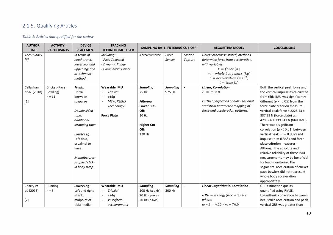
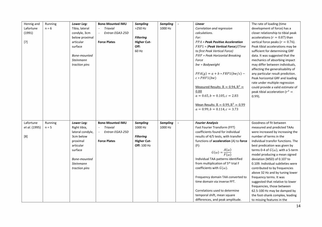
Table 1: Articles that qualified for the review. .................................................................................. 10
Table 2: The best correlations obtained within studies that used linear models to relate
acceleration with GRF. ....................................................................................................................... 30
Table 3: Variables used in the qualified articles for modelling the force-acceleration relationship. 36
Table 4: Variables taken from the force waveform to use in modelling the acceleration-force
relationship. ....................................................................................................................................... 42
Table 5: Variables taken from the acceleration waveform to use in modelling the acceleration-
force relationship. .............................................................................................................................. 42
Table 6: Additional variables considered in the qualifying articles. .................................................. 42
Table 7: Technologies utilised by the qualified articles. .................................................................... 47
Table 8: Attachment locations used in the qualified articles. ........................................................... 49
Table 9: Dynamic ranges of the devices used in the qualified articles. ............................................. 51
Table 10: Classification of correlation coefficients in sport-biomechanics as according to Hopkins
(2006). Reprinted with permission from William Hopkins. ............................................................... 57
Table 11: The best correlations between acceleration and GRF as presented within each of the
qualified articles. ................................................................................................................................ 58
Table 12: Instructions given to participants for completion within the study. ................................. 76
Table 13: Valid trials, according to movement type, participant, foot, and force plate. .................. 77
Table 14: Force variables and events considered in this investigation. ............................................ 89
Table 15: Acceleration variables and events considered in this investigation. ................................. 89
Table 16: Event-to-Event correlations for Participant 2 at the shank, 𝑅2 > 0.3. ............................. 90
Table 17: Correlations between the integration of force and acceleration. ..................................... 93
Table 18: Extension of Table 17, showing the cohort mass-induced correlation differences. ......... 94
Table 19: Comparison of correlation coefficients between 20 and 50 Hz filtered data. Green
indicates a stronger correlation. ........................................................................................................ 99
Table 20: Results of the linear Leave-One-Out investigation. ......................................................... 104
Table 21: Logarithmic models and respective correlations. ............................................................ 108
Table 22: Logarithmically modelling the vertical force and axial acceleration of Participant 4 at
each location. ................................................................................................................................... 109
Table 23: Logarithmically modelling the vertical force and axial acceleration of the entire cohort at
each location. ................................................................................................................................... 112
Table 24: Correlation and RMSE results of non-linear input-output waveform modelling. ........... 116

viii
Table 25: Correlation and RMSE results of non-linear input-output waveform modelling, where
mass has been included as an input. ............................................................................................... 117
Table 26: Correlation and RMSE results of non-linear input-output waveform modelling. ........... 118
Table 27: Correlation and RMSE results of non-linear input-output waveform modelling, where
mass has been included as an input. ............................................................................................... 118
Table 28: Individual participant thigh correlations. ......................................................................... 149
Table 29: Individual participant shank correlations......................................................................... 149
Table 30: Individual participant ankle correlations. ........................................................................ 150
Table 31: All Participants combined at each location: Part 1. ......................................................... 150
Table 32: All Participants combined at each location: Part 2. ......................................................... 151
Table 33: Participant-modelled logarithmic results......................................................................... 152
Table 34: Cohort-modelled logarithmic results. .............................................................................. 153

ix
List of Figures
Figure 1: Number of hospitalisations of children in Australian sport between 2005-2013 (Schneuer
et al., 2018). Reprinted with permission under CC BY 4.0. .................................................................. 2
Figure 2: Article Screening Process. ..................................................................................................... 8
Figure 3: The location of the IMU placements in the qualified articles. ........................................... 22
Figure 4: The sum of the primary, secondary, and tertiary acceleration frequency components
(bold) of the raw signals of the (A) foot and (B) shank (Takeda et al., 2009). Reprinted with
permission from Elsevier.................................................................................................................... 24
Figure 5: The publishing of the qualified articles and their algorithm models.................................. 28
Figure 6: (A) Vertical GRF and (B) tibial axial acceleration, during the stance phase of a cyclic
running activity at 4.5 ms-1 (Hennig and Lafortune, 1991). Reprinted with permission from Human
Kinetics, Inc. via Copyright Clearance Centre Inc. .............................................................................. 29
Figure 7: Prediction of GRF using tibial acceleration for three subjects on the left and right shank
(Charry et al., 2013). Reprinted with permission from IEEE © 2013 IEEE. ........................................ 31
Figure 8: Portion of studies that used triaxial vs. uniaxial devices. ................................................... 39
Figure 9: Calculating load rates in the vicinity of the first local maximum (Futrell et al., 2020).
Reprinted with permission under CC BY-NC-ND 4.0. ......................................................................... 43
Figure 10: GRF and vertical peak accelerations using commercial accelerometers, in 𝜇 ± 𝜎 (Meyer
et al., 2015). Reprinted with permission from Taylor & Francis. ....................................................... 48
Figure 11: The sampling rates used across the qualified articles. ..................................................... 53
Figure 12: Sports used in the qualified articles. Activities have been grouped according to
similarity. ............................................................................................................................................ 60
Figure 13: The activities trialled within the study from Meyer et al. (2015). Reprinted with
Permission from Taylor & Francis. ..................................................................................................... 61
Figure 14: Comparison of ground reaction force between soft and stiff surfaces (Devita and Skelly,
1992). Reprinted with permission from Wolters Kluwer Health, Inc. ............................................... 66
Figure 15: Force plate and motion capture utilisation. ..................................................................... 78
Figure 16: The location and orientation of the six trial devices. ....................................................... 79
Figure 17: Force plate noise fluctuation (N). ..................................................................................... 82
Figure 18: Raw resultant force and axial acceleration data of Participant 2. Local maximums
indicate the presence of noise. .......................................................................................................... 83
Figure 19: Raw data power spectra of (A) resultant force and (B) axial acceleration. ...................... 84
Figure 20: An analysis of noise in the raw resultant force data of a trial from Participant 2. .......... 84

x
Figure 21: Scaled-up power spectrum of Force M. ............................................................................ 85
Figure 22: Scaled-up power spectrum of Acceleration X. .................................................................. 86
Figure 23: Power spectra pre- and post-filtering of (A) resultant force and (B) axial acceleration. . 86
Figure 24: Force and acceleration before and after filtering (scaled). .............................................. 87
Figure 25: The force and acceleration events identified for analysis. ............................................... 88
Figure 26: The integrals (the area under the curves) of resultant and vertical (A) force and (B)
acceleration. ....................................................................................................................................... 88
Figure 27: Colour grading of correlations. ......................................................................................... 90
Figure 28: Correlations between resultant force and resultant acceleration at the shank. ............. 91
Figure 29: Correlations between resultant force and resultant acceleration at the thigh. .............. 92
Figure 30: Integration of the vertical force and axial acceleration waveforms................................. 93
Figure 31: Mass-scaled integral correlations. (A) Vertical force (ZINTEG) and axial acceleration
(XINTEGMASS). (B) Resultant force (MINTEG) and resultant acceleration (MINTEGMASS). ............ 95
Figure 32: Correlation differences after scaling by mass for resultant force (MMAX) and resultant
acceleration (MMAX). (A) Direct correlations. (B) Mass-scaled correlations. .................................. 96
Figure 33: Comparison of raw, 50 Hz filtered, and 20 Hz filtered acceleration data. ....................... 98
Figure 34: Flow-structure for the cross-validation protocol. ........................................................... 102
Figure 35: Developing a global model for the integration of force (impulse) from the data of
Participants 1 to 3. ........................................................................................................................... 102
Figure 36: Predicting the vertical force integral. (A) Predicting the force integration of Participant 4
from the developed model. (B) The correlation between predicted vs. actual force integration
values for Participant 4. ................................................................................................................... 103
Figure 37: Rectifying negative vertical force (ZMIN). (B) Original fit. (A) Rectified fit. ................... 106
Figure 38: Logarithmic prediction of force (ZMIN) from acceleration (XMAX) against the actual
value. ................................................................................................................................................ 107
Figure 39: Comparison of linear and logarithmic correlations between vertical force (ZMIN) and
axial acceleration (XMAX). (A) Participant 1. (B) Participant 2. (C) Participant 3. (D) Participant 4.
.......................................................................................................................................................... 107
Figure 40: Using linear approximations to obtain coefficients for the global logarithmic model. (A)
a(m). (B) b(m). .................................................................................................................................. 108
Figure 41: Comparison of the linear and logarithmic models for vertical-axial shank prediction. . 109
Figure 42: Cohort correlation of peak vertical force (MMAX) with peak axial acceleration (XMAX).
(A) Comparison of correlations. (B) Cohort 𝐹𝑉(𝑚, 𝐴𝑋) predicted fit against the actual force. ..... 110

xi
Figure 43: Adjusted predicted cohort fit.......................................................................................... 111
Figure 44: Non-linear input-output network design........................................................................ 114
Figure 45: Non-linear network training. Vertical axes: force (N). Horizontal axes: time in samples,
where 1 sample equals 0.5ms. ......................................................................................................... 115
Figure 46: Correlation of input and output samples following the waveform prediction. ............. 116
Figure 47: Factors that contribute to model predictions, ascertained from the literature. ........... 129
Figure 48: Conceptualising the long-term goal of this research - a risk scale generated for resultant
peak force. ....................................................................................................................................... 136

1
Chapter 1. Introduction
1.1. Introduction
This chapter frames the thesis by providing a brief understanding the development of overuse
injuries and by identifying the potential for such injuries to be prevented or monitored through the
development of a wearable device. The sport of focus within this investigation has been selected as
netball.
1.1.1. Injuries
A primary cause of stress fractures in the lower limb is inadequate adaption to repetitive cyclic
loading (Brukner and Bennell, 2020). As ground reaction force (GRF) strains the bone,
microdamage accumulates in weaker regions, with excess strain leading to fatigue reaction and
failure (Brukner and Bennell, 2020). Investigations have been undertaken to consider the
contribution of excess fatigue and loading rates to injury development, and to determine how
these characteristics can be measured with wearable devices in runners (Kiernan et al., 2018) and
team-sports such as Australian football (AFL) (Colby et al., 2014), soccer (Ehrmann et al., 2016),
and rugby (Gabbett and Ullah, 2012).
Studies like these have concluded that variables such as system acceleration, movement velocity,
and total distance covered during training sessions and gameplay may provide risk indicators for
overuse injuries and fatigue. The research is particularly relevant to the injury management of
female netballers. As shown in Figure 1, injury proportion by number of female hospitalisations in
netball and handball has been found to be the highest of all sports (Schneuer et al., 2018). It has
been further reported by Netball Australia that “netball is the activity with the second largest adult
female participation rates (89%), behind Pilates (90%)” (Netball Australia, 2019).

2
Figure 1: Number of hospitalisations of children in Australian sport between 2005-2013 (Schneuer et al., 2018).
Reprinted with permission under CC BY 4.0.
Within netball, the incidence of fatigue and overuse related injuries has been reported in elite
players at 9.08 (Best, 2017) and 23.8 (Hume and Steele, 2000) per 1000 hours of game play, and
14 per 1000 hours in non-elite players (McManus et al., 2006).0F
1 In one study, the incidence rate of
injury in elite and non-elite participants over the 5 consecutive years of a 14-week competition
was 5.4% (Hopper et al., 1995), and in the 1988 Australian Netball Championships, overuse injuries
were sustained by more than 25% of elite participants (Hopper and Elliott, 1993), where it was
seen that playing level had little effect on the number of players injured. Interestingly and perhaps
unsurprisingly, these injuries are not evenly distributed throughout the body.
In studies that have monitored netball injuries, a proportional 92.6% (Hopper et al., 1995) and 66%
(McManus et al., 2006) of injuries are reported as having occurred in the lower limb. When Bissell
and Lorentzos (2018) considered a cohort of 37 players, they found that lower limb injuries were
prevalent in 75% of players, with an equal prevalence of knee (47.2%) and ankle (47.2%) injuries
1 Consider that in the case of 23.8 injuries per 1000 hours (1 injury per 42 hours), if an elite player is training at this higher-risk level for 5 hours per week, this could mean experiencing an injury after just over 8 weeks.

3
across all players. Best (2017) reported that over a third of the total injuries were sustained in the
ankle, and Hopper et al. (1995) found the proportion to be 84.3%.
Best (2017) found that injuries were more commonly sustained during competition, with 71.2% of
all injuries in their study occurring in matches rather than during training. One may consider
whether all kinds of high intensity training is therefore hazardous, but although Stevenson et al.
(2000) related higher damage levels with greater exposure periods in training and match time
combined, McManus et al. (2006) found that training for four or more hours per week was
actually protective against injury. Indeed, there seems to be a level of training desirable for
strength-training and protection, yet over which injuries do become prevalent (Gabbett and Ullah,
2012).
Hopper et al. (1995), considering competitive matches only, reported that only 5% of injuries
required medical attention from a health care professional; whereas Stevenson et al. (2000), who
considered match and training time, reported that 20% of injuries required such attention. Best
(2017) even found a significant association between match quarter and injury occurrence (𝑝 =
0.019), with peak incidence occurring in the third quarter. As to when incidence increases during a
season, Best (2017) found that 57.6% of injuries had occurred in the first half of the season,
whereas over a similar period, Bissell and Lorentzos (2018) observed ankle injury prevalence to
increase. This may concur with Colby et al. (2014), who found that in elite footballers, three-
weekly cumulative loads were the most indicative of injury risk, rather than a long-term outlook
on summation.
These results indicate that injuries are prevalent among elite and non-elite athletes alike, with
variable incidence rates among both cohorts. Injuries sustained to netball players are found
primarily located in the lower limb, and commonly located at the ankle. Risk is seen to increase
within games, seemingly indiscriminately of point throughout the season, with injuries generally
increasing with greater exposure periods. However, exposure can also contribute towards
strength building and protective benefits, without necessarily increasing risk, meaning that load
monitoring may be valuable in both injury prevention and strength-training.
Although the exact benefit of wearable devices in this area is still being determined, it has been
observed that “an increase in peak acceleration might indicate higher loading rates, a reduction in
shock absorption quality and a higher impact on the body” (Reenalda et al., 2016). If this is so, and
an accurate relationship between acceleration and impact can be defined, then wearable

4
accelerometers could be used as tools to record acceleration, and this acceleration could be used
as a proxy for impact. Furthermore, if wearable accelerometers can be used to quantify impact
dose, then they may be beneficial in overuse injury management, by producing consistent, valid,
and accessible methods of impact dose and injury risk.
1.1.2. Considering a Device
Any device that is to be developed for targeting load management and injury prevention in
netballers must be grounded not only in the physiological relationship between impact force and
acceleration; and in literature-based design recommendations; but also in an understanding of the
desires and needs of current athletes. Therefore, an experienced, professional coach of an elite
netball team in the Netball SA (South Australia) Premier League was initially consulted for insight
on behalf of current athletes. This discussion, the conclusions of which are given below, included
two main considerations: injury prevention, and location and attachment.
Injury Prevention
It was explained by the coach that as players fatigue, the prevalence of injuries increases due to
heavier landings and less controlled movements. Inefficient recovery rates tend to bring structures
to failure, especially when participating in multiple activity sessions per week. As such, an ideal
device would provide quantitative, objective reasoning for why a player should not persist in
training when persistence may cause them to develop an injury. It would aid in the prevention of
future injuries, use previous injury data to indicate risk, and enable players to rate their feelings
subjectively. This would include promoting efficient recovery from past injuries and high amounts
of activity, informing the decision to rest and recover rather than persist until injury. This would be
quantified as a recovery level and would be used to inform safe training intensity and variety.
The primary desirable within an interface would be an alert system on increases to injury risk. The
device would indicate whether visual observations by coach and player are consistent with the
objective data. The interface would be user-friendly and provide only necessary information on
performance and injury risk, allowing all involved to focus on training, only needing to consider the
data when risk has developed. Ideally, the device would be used during training and matches.
Location and Attachment
The device would be small, developed such that it could be worn according to South Australian
and Australian Netball regulations. A suitable location such as the ankle would need to be selected

5
such that the device is minimally obstructive, easily accessible, and not hazardous during
gameplay. As players do not ordinarily wear compression tights, the device could not be placed
under tights or sleeves worn over the legs. However, if tights were necessary, then although
players might wear them during training, it is less likely that they would wear them during games;
although ultimately, the players would wear what is necessary for injury prevention.
Players tend to wear ankle-length socks, but crew socks may be worn when their ankle is strapped.
Because injuries are prevalent, most players strap or brace their ankles and knees each game for
both prevention and treatment, even if they are not currently injured. Players commonly use the
stirrup and heel-lock techniques for strapping ankles, using under-wraps of rigid Elastoplast. The
coach explained that similar techniques may be suitable for a new device. Since players do not use
leggings or straps except at the ankles and knees, a device that requires strapping in an abnormal
position may not be welcomed, allowed, or used by players. As such, although a device may be
fitted on mid-shank during trials, it is unlikely that a device placed here would remain when
competing. Ideally, the device would be placed medial or lateral to the central axis of the leg;
above the ankle, slightly caudal from the medial malleolus or the lateral malleolus; around the
sock line, akin to a watch placed on the wrist; this location would likely be acceptable.
The aesthetics of the device are also important, and a device that is not aesthetically appealing
would not likely be welcomed, even if it were technically approved. It was also acknowledged that
the development of a device in this area may require trial and error, testing for device profiles,
usability, and comfort.
Summary
In light of the high prevalence of injuries in elite and non-elite players alike, there remains a need
for an accessible method of injury management and prevention. The application of a wearable
accelerometer may provide this. Due to the high rate of lower limb injuries, and with the need for
a regulation-approved device, a device inferior on the body seems the most suitable, and
therefore will be the focus of this investigation. In the chapters that follow, a clear objective for
this investigation will be defined, the literature will be reviewed and synthesised, and conclusions
will be provided towards the search for an accessible method of lower-limb injury prevention.

6
1.2. Defining the Thesis Objective
This section states the aim of the thesis and a brief method for undertaking the investigation.
1.2.1. Aim
The aim of this research thesis is to establish an answer to the following question:
Is data collected from wearable accelerometers placed on the lower limb sufficient to model an
effective and useful relationship between ground reaction force and acceleration that is
generalisable between different subjects, movements, and external conditions?
Divided into five primary research areas, this project will aim to:
1. Determine whether there is a relationship between force and acceleration at the lower
limb.
2. Determine whether this relationship can be accurately modelled using data collected from
wearable accelerometers.
3. Determine whether this relationship is generalisable between subjects, movements, and
external conditions.
4. Determine whether measuring acceleration at the lower limb using wearable
accelerometers can provide data that is useful for the prevention or monitoring of injuries,
fatigue, and rehabilitation.
5. Determine information on the running of a trial such that new data can be collected, and a
relationship derived, based on the recommendations and performance of these studies.1F
2
1.2.2. Method
This investigation will be conducted in three parts, the methods of which will be further explained
throughout the thesis.
• Firstly, a systematic review of current literature regarding the topic will be undertaken, and
information synthesised for conclusions towards the research aims (Chapters 2 - 6).
• Secondly, an investigation will be undertaken in which previous data will be analysed based
on insights gained from the literature (Chapter 7).
• Finally, a discussion will consider and conclude on the results of the literature review and
investigation (Chapter 8-9).
2 If retrievable, this information will include insight on device development, attachment methods, and data analysis.

7
Chapter 2. Literature Review
2.1. Methods and Search
This chapter explains the method by which the literature in this thesis was investigated. It explains
why certain articles have been included and excluded, and it tabulates the articles that qualified as
primary sources.
2.1.1. Terms and Protocol
Articles qualified for this review if they provided an understanding on four key areas: wearable
devices, the lower limb, acceleration, and force. As such, the following search term was developed
to retrieve articles inclusive of this information:
wearable AND (ankle OR shank OR "lower limb") AND acceler* AND force
This search term was queried in six relevant databases: Medline, Scopus, PubMed, IEEE, ProQuest
and Science Direct. Script was written in MATLAB to sort between unique titles within the search
results of each database. Across the six databases, 154 individual titles were retrieved, from which
99 articles were unique. Each unique title was reviewed based on title, abstract and potential
relevance to the discussion, and 76 articles were selected for further review. From these 76
articles, 5 qualified for the review. An additional 11 articles were also included in the review: 5
were identified within the reference lists of the qualified articles, and 6 were obtained through
external sources. This process has been illustrated in Figure 2.

8
Figure 2: Article Screening Process.
2.1.2. Exclusion Criteria
The following criteria were used during both the screening and the refine process to exclude
articles as primary sources. Articles were excluded if they:
• Did not collect acceleration data using an accelerometer.
o Articles were included if they measured acceleration but did not specify the device
as an accelerometer, or if the device used was a multifunction device i.e. if a study
used terms such as inertial measurement unit (IMU).
• Did not consider the placement of the accelerometer in relation to the lower limb.
o Articles were included if the accelerometer was not placed on the lower limb, but
only if they provided insight into the effectiveness of this placement with regards to
kinematics of the lower limb.
• Did not use acceleration to predict ground reaction force.
o Articles were excluded if they used acceleration data to predict power or impulse.
• Were not articles that included a trial.

9
o Articles were excluded if they were reviews, discussions, trial proposals or device
introductions.
• Were not written in English.
2.1.3. Additional Articles within the Discussion
During the article selection, although articles were excluded, relevant and valuable information to
this discussion was noted and included in the synthesis. Of these non-qualifying articles from
which information was included, they were predominantly obtained though the original database
search. The synthesis also includes articles identified through the references of these articles and
from additional external sources.
2.1.4. Information Collected in the Review
Information collected on the qualifying articles has been given in Table 1.
• Articles have been numbered sequentially in Table 1 as [𝑥]; these numbers are referred to
by infographics within this thesis, and where possible have been hyperlinked accordingly.
• Device placement sites were arbitrarily classified as either the head, neck, trunk, upper leg,
or lower leg. Where possible, detailed locations and attachment methods have also been
included.
• Articles are classified as having used a kind of inertial measurement unit (IMU). ‘IMU’ has
been used as a broad term for any device that collected acceleration data from the subject.
In some cases, gyroscopes, magnetometers, and other sensors were also present within
the device.
• Sampling rates and filtering cut-off frequencies have been included where possible. This
will be discussed in further detail in the synthesis to follow, but it must be noted that filters
between studies varied in kind and order (i.e. 4th order Butterworth etc.); only the cut-off
frequencies have been specified within this table.
• Force Sensor has been used as a generalised term for whichever force sensor was used in
the investigation. It covers force plate, instrumented treadmill, and pressure-sensing insole.
• The algorithm models specified do not necessarily explain every process used within each
study. They have merely been included in an attempt to describe the fundamental
techniques that were used to model the data within each study.
• Algorithm classifications have been classified as linear, logarithmic, Fourier, non-linear etc.
The articles within this table will henceforth be referred to as the qualified articles.
10
2.1.5. Qualifying Articles
Table 1: Articles that qualified for the review.
AUTHOR,
DATE
ACTIVITY,
PARTICIPANTS
DEVICE
PLACEMENT
TRACKING
TECHNOLOGIES USED SAMPLING RATE, FILTERING CUT-OFF ALGORITHM MODEL CONCLUSIONS
Thesis Index
[#]
In terms of
head, trunk,
lower leg, and
upper leg; and
attachment
method.
Including:
- Axes Collected
- Dynamic Range
- Commercial Device
Accelerometer Force
Sensor
Motion
Capture
Unless otherwise stated, methods
determine force from acceleration,
with variables:
𝐹 = 𝑓𝑜𝑟𝑐𝑒 (𝑁)
𝑚 = 𝑤ℎ𝑜𝑙𝑒 𝑏𝑜𝑑𝑦 𝑚𝑎𝑠𝑠 (𝑘𝑔)
𝑎 = 𝑎𝑐𝑐𝑒𝑙𝑒𝑟𝑎𝑡𝑖𝑜𝑛 (𝑚𝑠−2)
𝑡 = 𝑡𝑖𝑚𝑒 (𝑠)
Callaghan
et al. (2018)
[1]
Cricket (Pace
Bowling)
n = 11
Trunk:
Dorsal
between
scapulae
Double sided
tape,
additional
strapping tape
Lower Leg:
Left tibia,
proximal to
knee
Manufacturer-
supplied click-
in body strap
Wearable IMU
- Triaxial
- ±16g
- MTw, XSENS
Technology
Force Plate
Sampling
75 Hz
Filtering
Lower Cut-
Off:
10 Hz
Higher Cut-
Off:
120 Hz
Sampling
975 Hz
- Linear, Correlation
𝑭 = 𝑚 × 𝒂
Further performed one-dimensional
statistical parametric mapping of
force and acceleration patterns.
Both the vertical peak force and
the vertical impulse as calculated
from tibia IMU was significantly
different (𝑝 < 0.05) from the
force plate criterion measure:
vertical peak force = 2228.43 ±
837.99 N (force plate) vs.
4295.66 ± 1393.41 N (tibia IMU).
There was a significant
correlation (𝑝 < 0.01) between
vertical peak (𝑟 = 0.832) and
impulse (𝑟 = 0.865) and force
plate criterion measures.
Although the absolute and
relative reliability of these IMU
measurements may be beneficial
for load monitoring, the
segmental acceleration of cricket
pace bowlers did not represent
whole body acceleration
appropriately.
Charry et
al. (2013)
[2]
Running
n = 3
Lower Leg:
Left and right
shank,
midpoint of
tibia medial
Wearable IMU
- Triaxial
- ±24g
- ViPerform:
accelerometer
Sampling
100 Hz (x-axis)
20 Hz (y-axis)
20 Hz (z-axis)
Sampling
300 Hz
-
Linear-Logarithmic, Correlation
𝑮𝑹𝑭 = 𝑎 ∗ log2(𝒂𝒄𝒄 + 1) + 𝑐
where:
𝑎(𝑚) = 4.66 ∗ 𝑚 − 76.6
GRF estimation quality
quantified using RMSE.
Logarithmic correlation between
heel strike acceleration and peak
vertical GRF was greater than

11
malleolus and
knee medial
joint line
Adhesive
sticker
LSM303DLHC from
ST
Microelectronics –
c.f. Penghai et al.
(2014)
Force Plate
𝑐(𝑚) = 24.98 ∗ 𝑚 − 566.83
𝑎𝑐𝑐 = 𝑚𝑎𝑥𝑖𝑚𝑢𝑚 𝑒𝑣𝑒𝑛𝑡
𝑡𝑖𝑏𝑖𝑎𝑙 𝑎𝑥𝑖𝑎𝑙 𝑎𝑐𝑐𝑒𝑙𝑒𝑟𝑎𝑡𝑖𝑜𝑛
Coefficients in equations a(m) and
c(m) were calculated empirically
based on the mass of the three
subjects.
linear correlation (𝑅2 =
0.95 𝑣𝑠. 0.81); correlation
differences were similar in initial
peak acceleration, maximum
peak acceleration and peak-to-
peak acceleration events.
Highest correlation for all
subjects between GRF and the
logarithmic acceleration function
occurred at the maximum
acceleration peak. Including
body mass in algorithm reduced
error by 30%. Different runners
at similar running speeds had
varied results. ViPerform, which
uses a single 3D accelerometer,
was concluded as viable for force
estimations outside the lab.
Davis et al.
(2018)
[3]
Running
n = 169
Lower Leg:
Left distal
medial tibia
-
Wearable IMU
- Triaxial
Instrumented
Treadmill
- -
-
Correlation
Load rates and accelerations over 8
consecutive steps were averaged and
then correlated.
All correlations were significant,
except resultant tibial
acceleration with vertical
instantaneous load rate in fore-
foot strike. All correlations were
between 0.37 to 0.82. Peak
vertical tibial acceleration was
correlated for all strike patterns
(𝑟 = 0.72, 𝑝 < 0.001). It was
concluded that vertical tibial
acceleration may be the best
surrogate for the load rate of
running impact.
Elvin et al.
(2007)
[4]
Jumping
n = 6
Lower Leg:
Left and right
shank, fibula
(over fibular
head)
Sleeve over
knee:
Wearable IMU
- Uniaxial
- ±70g
- ADXL78, Analog
Devices Inc.
Force Plate
Sampling
1000 Hz
Sampling
1000 Hz
-
Correlation
Acceleration jump data from both
legs were averaged and interpolated
for a single record.
The algebraic mean of the TAA was
related to the single GRF output of
the force plate.
Across subjects, average 𝑟2 for
Peak vertical GRF and Peak TAA
was strong and significant (𝑟2 =
0.812, 𝑝 ≤ 0.01); likewise
between jump height (force) and
jump height (acceleration) (𝑟2 =
0.879, 𝑝 ≤ 0.01). Jump height
did not correlate with peak

12
Drytex Knee
Support
Coefficients of determination (𝑟2)
calculated by standard linear least
square correlation for:
1. Peak impact vertical GRF vs.
peak impact tibial axial
acceleration
2. Jump height (force) vs. jump
height (acceleration).
3. Peak impact force vs. jump
height (force)
4. Peak impact acceleration vs.
jump height (acceleration)
Jump Height calculations:
𝐻 = 𝑔𝑡2/8
Where 𝑡 = total flight time:
- In (force) calculation, 𝑡 = the
time between when GRF = 0
(i.e. when the body is not
touching the plate).
- In (acceleration) calculation,
𝑡 = the time between when
𝑎 = −𝑔.
impact force (𝑟2 = 0.127) or
peak impact acceleration (𝑟2 =
0.119). Errors may be present
due to tibia-impact line angle.
The dynamics of skin motion
with sleeve slipping were
discounted due to intra-
participant consistency. When
the force along the X and Y axes
are ignored, a maximum 20%
error is observed in the tibial axis
GRF.
Guo et al.
(2017)
[5]
Walking
n = 9
Trunk:
L5 vertebra
-
Neck
C7 vertebra
-
Head
Forehead
-
Wearable IMUs
- Triaxial
- ±6g
- Opal™, APDM Inc.
Pressure-Sensing
Insoles
Sampling
128 Hz
Sampling
128 Hz
- Non-Linear Model
64-term Non-linear AutoRegressive
Moving Average with eXogenous
input (NARMAX) model obtained to
predict vertical GRF of right and left
feet:
𝒗𝑮𝑹𝑭
= ∑𝜃𝑖𝜙𝑖(�⃗⃗� 𝒔𝒆𝒏𝒔𝒐𝒓(𝒌), �⃗⃗� 𝒔𝒆𝒏𝒔𝒐𝒓(𝒌
𝑛
𝑖
− 𝟏),… , �⃗⃗� 𝒔𝒆𝒏𝒔𝒐𝒓(𝒌 − 𝑳))
This considers:
- Gravity
- Time-varying accelerations
- Time-varying orientations
Mean error from L5 position for
outdoor controlled walking was
3.8%, with cross correlation
coefficient of 𝜌=0.993 (p<0.01).
Mean error from L5 position for
outdoor free walking was 5.0%
with cross correlation coefficient
𝜌=0.990 (p<0.01).
Model prediction errors were
minimum in the L5 model
compared to C7 and forehead.
C7 model had the smallest inter-
subject variability and a more
stable performance than the
other proxy models. However,
the performance of the proxy

13
- Associated time delays
- Decomposition of left and
right components of gait
signal
The data based on individual sensors
using an iterative orthogonal
forward regression algorithm. It
models both feet vertical GRF
separately from the single
accelerometer, based on its
membership in the gait cycle.
models was similar in all
locations.
Havens et
al. (2018)
[6]
Running
n = 14
Upper Leg:
Left and right
thigh, between
lateral
epicondyle and
greater
trochanter
Lower Leg:
Left and right
shank,
between
lateral
malleolus and
lateral
epicondyle of
femur
Both:
Nylon elastic
band wraps;
under semi
rigid plastic
plates; under
elastic straps
under duct
tape.
Wearable IMU
- Triaxial
- Opal™, APDM Inc.
Force Plates
Motion Capture
Sampling
128 Hz
Filtering
Higher Cut-
Off:
12 Hz
Sampling
1360 Hz
Sampling
340 Hz
Correlation
Stepwise regressions calculated for
between-limb accelerations in the
shank and thigh between loading
and power.
Between limb differences in
surgical vs non-surgical limbs
indicated that greater
differences in thigh axial
acceleration was related to
greater differences in GRF and
knee power absorption. Axial
acceleration predicted knee
power absorption and deficits in
surgical limbs were observed.
Thigh acceleration correlated
more strongly with GRF than
tibial acceleration. Relationships
were not identified between
knee mechanics and shank
acceleration. Shank acceleration
may not be as useful as thigh
acceleration for knee joint
power, but each may provide
information on knee loading
deficits.
14
Hennig and
Lafortune
(1991)
[7]
Running
n = 6
Lower Leg:
Tibia, lateral
condyle, 3cm
below proximal
articular
surface
Bone-mounted
Steinmann
traction pins
Bone-Mounted IMU
- Triaxial
- Entran EGA3-25D
Force Plates
Sampling
>250 Hz
Filtering
Higher Cut-
Off:
60 Hz
Sampling
1000 Hz
- Linear
Correlation and regression
calculations.
For:
𝑃𝑃𝐴 = Peak Positive Acceleration
𝐹𝑅𝑃1 = (Peak Vertical Force)/(Time
to first Peak Vertical Force)
𝑃𝐻𝐹 = Peak Horizontal Breaking
Force
𝑏𝑤 = Bodyweight
𝑃𝑃𝐴(𝑔) = 𝑎 + 𝑏 ∗ 𝐹𝑅𝑃1(𝑏𝑤/𝑠) −
𝑐 ∗ 𝑃𝐻𝐹1(𝑏𝑤)
Measured Results: R = 0.94, R2 =
0.88
𝑎 = 0.65, 𝑏 = 0.105, 𝑐 = 2.83
Mean Results: R = 0.99, R2 = 0.99
𝑎 = 0.99, 𝑏 = 0.114, 𝑐 = 3.73
The rate of loading (time
development of force) has a
closer relationship to tibial peak
accelerations (𝑟 = 0.87) than
vertical force peaks (𝑟 = 0.76).
Peak tibial accelerations may be
sufficient for determining GRF
data. It was suggested that the
mechanics of absorbing impact
may differ between individuals,
affecting the generalisability of
any particular result prediction.
Peak horizontal GRF and loading
rate under multiple regression
could provide a valid estimate of
peak tibial acceleration (𝑟2 =
0.99).
Lafortune
et al. (1995)
[8]
Running
n = 5
Lower Leg:
Right tibia,
lateral condyle,
3cm below
proximal
articular
surface
Bone-mounted
Steinmann
traction pins
Bone-Mounted IMU
- Triaxial
- Entran EGA3-25D
Force Plates
Sampling
1000 Hz
Filtering
Higher Cut-
Off: 100 Hz
Sampling
1000 Hz
- Fourier Analysis
Fast Fourier Transform (FFT)
coefficients found for individual
results of 4/5 tests, with transfer
functions of acceleration (A) to force
(F):
𝐺(𝜔) =𝐴(𝜔)
𝐹(𝜔)
Individual TAA patterns identified
from multiplication of 5th trial F
coefficients with 𝐺(𝜔).
Frequency domain TAA converted to
time domain via inverse FFT.
Correlations used to determine
temporal shift, mean square
differences, and peak amplitude.
Goodness of fit between
measured and predicted TAAs
were increased by increasing the
number of terms in the
individual transfer functions. The
best predication was given by
terms 0-4 of 𝐺(𝜔), with a 5-term
model producing a mean signed
deviation (MSD) of 0.107 to
0.109. Individual subtleties were
contributed to by frequencies
above 32 Hz and by tuning lower
frequency terms. It was
suggested that relative to lower
frequencies, those between
62.5-100 Hz may be damped by
the foot-shank complex, leading
to missing features in the

15
4/5 participant results combined for
a generic transfer function by which
5th participant results then
calculated; process repeated for
each participant.
Finally, a general 𝐺(𝜔) calculated
from all results. Term coefficients
within study.
individual functions. However,
these functions lacked bias and
as such should be externally
generalisable under similar
conditions.
Meyer et al.
(2015)
[9]
Various Tasks
n = 13
Walking,
jogging,
running,
landings, jump
rope, dancing.
Upper Leg:
Right hip
-
Wearable IMU
- Triaxial
- ±6g
- ActiGraph GT3X,
ActiGraph; (ACT)
- Triaxial
- ±8g
- GeneActive,
ActiveInsights;
(GEN)
Force Plates
Sampling
100 Hz
Sampling
2400 Hz
- Linear
Vertical GRFs calculated with:
𝑭 = 𝑚 × 𝒂
Acceleration datasets between IMUs
were synchronised by matching to
the point of highest cross-
correlation.
Minimum acceleration values were
averaged per step and per trial
Observed the differences in
regression analyses between sex,
age, weight, height, and leg length.
Considered differences when values
which peaked the dynamic range
were included or excluded.
Considered only values with little
variance.
“Data from ACT and GEN
correlated with GRF (r = 0.90 and
0.89, respectively) and between
each other (r = 0.98).” GRF
increased significantly from
walking to jogging to running
(Pearson correlation <0.001) and
landing tasks (10-30cm) also
produced significantly higher
GRF than in walking, jogging, and
running tasks (P<0.014). Rope
skipping GRF corresponded to
GRF from 10cm landing tasks.
Both accelerometers significantly
and systematically
overestimated GRF from their
acceleration values. Systematic
bias of ACT was 0.46g and GEN
1.39g. Measurement bias was
found to increase with higher
loadings.
Penghai et
al. (2014)
[10]
Jumping
-
Trunk:
Posterior,
centre of waist
-
Wearable IMU
- Triaxial
- ±6g
- LIS3LV02DL
STMicroelectronics
Sampling
640 Hz
(down
sampled to
400 Hz)
- - Linear
Gyroscope angular output used to
determine rate of change, which is
used to determine acceleration in the
vertical axis.
As measured by Myotest, the
results between the IMU and the
HUR force platform were weakly
correlated.

16
Force Plate
Filtering
Higher Cut-
Off:
30 Hz
Total Valid Acceleration:
𝒂𝒗𝒂𝒍𝒊𝒅 = 𝑎𝑥 cos(𝜃1) cos(𝜃2) +
𝑎𝑦 sin(𝜃1) + 𝑎𝑧 sin(𝜃2)
Maximum Jumping Force:
𝑱𝑭𝑴𝑨𝑿 = 𝑚 ∙ 𝑀𝐴𝑋⟨𝐴𝑡⟩
Maximum Explosive Jump Power:
𝐸𝑃𝑀𝐴𝑋 = 𝑚 ∙ 𝑀𝐴𝑋 ⟨𝑎𝑡 ∙
(∫ 𝑎𝑡𝑑𝑡𝑡
𝑡−𝑡0+ 𝑉𝑡−𝑡0)⟩
Maximum Height:
𝐻𝑀𝐴𝑋 = 𝑡0 ∙ 𝑀𝐴𝑋 ⟨∑ 𝑉𝑡
𝑡
0⟩
FIR low-pass filter cut-off was further
applied at 30 Hz.
Numerical correlations were not
given.
Pieper et al.
(2020)
[11]
Walking
n = 12
Lower Leg:
Left and right
Anterior tibia,
50% of shank
length.
-
Wearable IMUs
- Triaxial
- Delsys TRIGNOTM
Instrumented
Treadmill
Motion Capture
Sampling
1000 Hz
-
Filtering
Higher
Cut-Off:
20 Hz
Sampling
100 Hz
Filtering
Higher
Cut-Off:
6 Hz
Linear
Correlations between peak shank
acceleration (g) and peak anterior
GRF (N) in normal gait and in gait
inhibited by a leg brace.
𝑦 = Peak Anterior GRF (N)
𝑥 = Peak Shank Acceleration (g)
For un-braced leg:
𝑅𝑖𝑔ℎ𝑡: 𝑦 = 241.7𝑥 + 6.9
𝑅2 = 0.77, 𝑃 < 0.001
𝐿𝑒𝑓𝑡: 𝑦 = 224.7𝑥 + 15.7
𝑅2 = 0.71, 𝑃 < 0.001
For braced leg:
Right: 𝑦 = 173.4𝑥 + 4.8
𝑅2 = 0.31, 𝑃 = 0.06
Changes modulated by GRF and
power output correlated with
proportional changes in
acceleration immediately
following push-off. Inducing an
impairment via a right knee
brace caused a systematic and
significant reduction in limb
propulsion. Braced leg peak
shank acceleration did not
correlate with peak anterior GRF
(𝑅2 = 0.31, 𝑝 = 0.061). Peak
shank acceleration had a
consistent temporal delay
following toe-off. A unilateral
leg-brace impairment does not
replicate neuromuscular
limitations present following
stroke. However, these results
may be beneficial for measuring
trailing-limb propulsion.

17
Raper et al.
(2018)
[12]
Running
n = 10
Lower Leg:
Medial border
of tibia 2F
3
Wearable IMUs
- Triaxial
- ViPerform v5
Force Plates
Sampling
100 Hz (x-axis)
20 Hz (y-axis)
20 Hz (z-axis)
Sampling
1000 Hz
Filtering
Higher
Cut-Off:
100 Hz
Sampling
200 Hz
-
Analysis performed with
manufacturer program Running
Analysis. Program algorithm strategy
method not given.
On testing the absolute reliability
of ViPerform, the device was not
found to calculate GRF similarly
to a force plate measurement.
ViPerform was found to have an
accuracy of 83.96%. However, it
had an intra-class correlation
coefficient of 0.877 (95%
confidence interval 0.825-0.915)
and as such was deemed
excellent. It was concluded that
the ViPerform calculates GRF
consistently but is not accurate
to reference Force Plates. As
such it may be useful as an
arbitrary load unit. The varying
sampling rates may cause the
ViPerform to be subject to
aliasing. Group data is unlikely to
assist measurement, and
individual baseline measures will
be required in future studies.
Simons and
Bradshaw
(2016)
[13]
Hopping-
Jumping-
Landing Tasks
n = 12
Trunk:
Upper back,
over second
thoracic
vertebra
Tight-fitting
crop top
Trunk:
Lower back,
midpoint of
superior iliac
spines of pelvis
Wearable IMUs
- Triaxial
- Minimaxx S4 GPS-
uni
Force Plates
Sampling
100 Hz
Filtering
Higher Cut-
Off:
8, 15, 20, 50
Hz
Sampling
500 Hz,
1000 Hz
Filtering
Higher
Cut-Off:
100 Hz
- Correlation
Peak resultant acceleration, peak
vertical GRF, peak resultant GRF
correlated.
PRA from the three trials of each
task were averaged. GRF was
normalised by body weight.
Significant differences were not
found in peak resultant
accelerations (PRA) between
drop heights of 57.5 cm and 77.5
cm in upper or lower back
placement. The strongest GRF-
PRA correlation for the hopping
task was found with a 15 Hz cut-
off at the lower back, and 8 Hz at
the upper back, both producing
Spearman’s rank correlation
coefficients (𝑟𝑠) of 𝑟𝑠 = 0.860.
Significant correlations were only
found in the lower back when
recorded from 37.5 cm. The
3 Mounting setup given according to Liikavainio et al. (2007).

18
Double-sided
tape Fixomull
stretch tape,
tight-fitting
leggings, or
compression
pants
significance of correlations
differed according to the cut-off
filters applied. Continuous
hopping acceleration (filtered at
20 Hz) had a correlation with
GRF of 𝑟𝑠 = 0.825. Overall, PRA
was considered a good estimate
of impact loading, especially
when recorded at the upper back
and filtered at 20 Hz. PRA was
able to accurately discriminate
between landing heights.
Tan et al.
(2020)
[14]
Running
n = 15
Trunk:
Upper Back, T5
vertebra
Trunk:
Pelvis, mid-
point between
left and right
anterior
superior iliac
spine
Upper Leg:
Left thigh, mid-
point between
left anterior
superior
iliac spine and
left femur
medial
epicondyle
Lower Leg:
Left shank, one
third point
between left
femur medial
epicondyle and
Wearable IMUs
- Triaxial
- MTi-300, Xsens
Technologies
Instrumented
Treadmill
Motion Capture
Sampling
200 Hz
Filtering
Higher Cut-
Off:
75 Hz
Sampling
1000 Hz
Filtering
Higher
Cut-Off:
50 Hz
-
Filtering
Higher
Cut-Off:
12 Hz
Convolutional Neural Network
(CNN)
- Foot contacts detection
algorithm segmented data into
discrete steps
- Gait cycle input to the CNN
model
- Acceleration-XYZ
- Gyroscope-XYZ
- Convolution operations
performed on data window and
kernels
- Pooling operations extracted
the maximum values
- Features fed into a fully
connected network, with:
- Two additional auxiliary
inputs
(swing phase duration and
stride duration)
- Three hidden dense layers
(activation function was a
rectified linear unit
function)
- One output layer
(activation function was an
identify function)
Correlations were strong
between running conditions,
speeds, footwear, strike patterns
and step rates (𝜌 ≥ 0.88). From
single sensors, correlations
between input and output
(VALR) were: Shank: 𝜌 = 0.94;
Foot: 𝜌 = 0.91; Pelvis: 𝜌 = 0.76;
Trunk: 𝜌 = 0.69; Thigh: 𝜌 =
0.65. Although insignificant,
there was an increase in
correlation as data from multiple
sensors was integrated (1
sensor: 𝜌 = 0.94(0.03); 5
sensors: 𝜌 = 0.96 (0.02)). The
shank was therefore deemed the
optimum location for impact
loading. It was said that the foot
is also an especially good
location since many commercial
devices already attach to the
foot. A larger and more general
population will enable a more
accurate vertical average loading
rate estimation model.

19
left tibia apex
of medial
malleolus near
proximal end
of tibia
Lower Leg:
Left foot, left
second
metatarsal
All IMUs
attached with
straps around
the body
segment
- Output variable: vertical
average loading rate (of the
resultant GRF waveform)
Tran et al.
(2012)
[15]
Landing-
Jumping
n = 10
Neck:
At the base of
the neck.
Manufacturer-
provided
harness
Wearable IMU
- Triaxial
- SPI Pro
Force Plate
Sampling
100 Hz
Filtering
Higher Cut-
Off:
20 Hz
Sampling
100 Hz
- Correlation
Vertical GRF values adjusted by body
weight and compared to filtered
accelerations (raw and smoothed).
Bodyweight adjusted c.f. (Simons
and Bradshaw, 2016) i.e. they
normalised the GRF rather than
multiplying acceleration by mass.
On comparing the commercial
device to the vertical GRF values
measured by the force plates, all
bodyweight adjusted peak
accelerations were significantly
higher than the vertical GRF
between landing tasks. (𝑝 <
0.05). However, moderate
correlations of 𝑟 = 0.45 to
0.70 (𝑝 < 0.05) were found
between these variables.
Smoothing this data led to
reduced variations in the data,
(within 10.9-22.2%). Since the
level of acceptability was
deemed 20%, this device was
considered able to quantify
impacts consistently, though not
from raw data.
Wundersitz
et al. (2013)
[16]
Running
n = 17
Trunk:
Centre of the
upper back,
approximately
above second
Wearable IMU
- Triaxial
- ±8g
- SPI Pro
Sampling
100 Hz
Filtering
Sampling
100 Hz
- Linear, Correlation
𝑭 = 𝑚 × 𝒂
There were weak to moderate
correlations (−0.26 < 𝑟 < 0.33)
across all cranial-caudal force
tasks. There was a strong
correlation for 0° change of

20
thoracic
vertebra.
Placed within a
mini-backpack,
within the
manufacturer-
supplied
harness.
Force Plate
Motion Capture
Lower Cut-
Off:
Higher Cut-
Off:
10, 15, 20, 25
Hz
direction (𝑟 = 0.76) and 45°
(𝑟 = 0.67). However, raw
accelerometer data significantly
overestimated resultant GRF at
the force plates (p < 0.01).
Measurement errors increased
with degree of change of
direction. However, smoothing
data at 10 Hz was found to
positively influence the results of
the movements performed.
There was an indication that
smoothed data may provide
acceptable agreement for force
prediction. Deviation of the IMU
from the vertical axis was a
major influence on the errors in
these results. Absolute errors for
single measurements were
between 12-24%.

21
Chapter 3. Modelling Activity Characteristics
Research Aim #1
Determine whether there is a relationship between force and acceleration at the
lower limb.
3.1. Recording at the Lower Limb
The qualified articles have examined the relationship between acceleration and ground reaction
force across several body segments during movement. If the ideals proposed in Chapter 1 are to be
verified, it must be determined whether this relationship can be modelled by data recorded at the
lower limb. As such, this chapter will consider three implications made in the literature regarding
placement at the lower limb: the locational accuracy of devices placed there, the attenuation and
distribution of impact forces throughout the body during movement, and relevant rules and
legislation for device placement as defined by Netball Australia and other sports.
3.1.1. Location
Research on wearable sensor systems may be divided into the recognition of daily activities and
the accurate measurement of human motion data (Abdelhady et al., 2019). Within these research
areas, there is a clear market opportunity for low-cost devices that are able to measure the
plantar and ground reaction forces of gait analysis at a high quality (Abdelhady et al., 2019). The
design of such wearable systems would allow users to analyse gait and movement kinetics,
without needing access to a laboratory (Jacobs and Ferris, 2015). Fulfilling this requires designing
these devices accurately both according to the location from which data is recorded and the
accuracy of captured metrics provided by each device.
Location Possibilities
Obtaining consistent accuracy has been a major hurdle in studies that have researched the
development of accurate wearable technologies, often due to the variance in results between
participants and locations (Elvin et al., 2007). To compensate for this, location protocols and
recommendations have been widely researched. Studies have considered acceleration in various
applications and locations, with many specifically considering its relationship to impact.
Accelerometers have been trialled on the feet (Takeda et al., 2009); the tibia (Tenforde et al.,

22
2020); the hip (Meyer et al., 2015); the lower back (Penghai et al., 2014) and upper back
(Wundersitz et al., 2013); the neck (Tran et al., 2012); the forehead (Guo et al., 2017); and even in
a plastic mouth piece (Lewis et al., 2001). This wide distribution provides the grounds for this
discussion on the benefits and difficulties of location. The placements considered in the qualified
articles have been illustrated in Figure 3.
Figure 3: The location of the IMU placements in the qualified articles.
Of the 15 different locations shown in Figure 3, there were 19 IMU placements on the lower half
of the body (the lower and upper leg), with 15 specifically on a lower leg. Often in the literature,
the lower leg was selected because of the findings of previous studies, or because of placement
assumptions. For example, Charry et al. (2013) selected the medial tibia on the recommendation
of Liikavainio et al. (2007), who had reported it an accurate site for recording acceleration. Elvin et
al. (2007) chose the fibular head since the prominent structure enabled placement repeatability
due to the obvious identification of the palpation; and because it was deemed low risk for injury

23
from falls; and because they had seen it done before (Puyau et al., 2002). Not aware of conclusive
evidence for optimal placement, Simons and Bradshaw (2016) assumed that assessing impact
loading during jumping and landing tasks would be best represented by the lower back, since this
is at the centre of mass. Since the literature review targeted the lower limb, it is unsurprising that
most of the IMUs were located here. However, the variance does provide insight into the effects
on accuracy between locations.
Rouhani et al. (2014) have demonstrated that forces and torques vary significantly across the
lower leg, depending on if measured at the shank, hindfoot, forefoot, or toes; and that moments,
powers, and forces differ in shape and magnitude between planes. This immediately indicates that
three-dimensional effects of segment position and rotation may prove helpful in model
development.3F
4 These effects are objectively seen between placement sites when considering
location-based correlations. Tan et al. (2020), who tested sensor locations on the body at the
trunk, pelvis, thigh, shank, and foot, found that the correlation differed between locations, and
was the highest for a single sensor when located on the shank, producing load rate correlation
coefficients of 𝜌 = 0.94. However, although this may seem optimal for modelling impact due to
the high correlation, the shank has been shown to record lower acceleration magnitudes than at
the foot (Takeda et al., 2009).
Waveform Differences
After performing a frequency decomposition on the acceleration signals at the abdomen, both
thighs, shanks and feet during walking, Takeda et al. (2009) observed that the signal was greatest
in magnitude at the feet, attenuating as it moved away from the point of impact. For example, as
shown in Figure 4, they found that there were high frequency, high magnitudes components
unique only to the foot.
4 The contribution of planes and axes of motion will be discussed further in Chapter 3.2.4.

24
Figure 4: The sum of the primary, secondary, and tertiary acceleration frequency components (bold) of the raw signals
of the (A) foot and (B) shank (Takeda et al., 2009). Reprinted with permission from Elsevier.
Since Tan et al. (2020) found that the shank was optimal for modelling load rates, but it is here
seen that the force magnitude attenuates away from the source of impact, force modelling may
depend not primarily upon the acceleration magnitude, but on the force-acceleration waveform
similarity.
And yet, even with the confidence of such studies that consider the shank an optimal
representation of ground reaction forces, location may not be the most crucial factor when
determining model efficacy. Guo et al. (2017) performed a study in which none of the locations
tested for IMU location were on the lower limb, and this was the study that produced the highest
correlation accuracy of the qualified articles, with a maximum cross correlation coefficient of 𝜌 =
0.993. Nevertheless, this does not invalidate the conclusions of other studies that have considered
the practical application of lower limb acceleration, since Guo et al. (2017) was one of only two
qualified articles to use a machine learning algorithm.4F
5 Nevertheless, location clearly still affects
the relationship. To understand this, the effects of force attenuation and distribution throughout
the body must be considered.
3.1.2. Attenuation
Attenuation is particularly important for modelling a relationship in the field of elite sport, since as
athletes improve in managing their shock attenuation, the effectiveness of using peak resultant
acceleration as a proxy for GRF can also increase (Simons and Bradshaw, 2016). Simons and
Bradshaw (2016) determined that the relationship between GRF and torso accelerations is likely to
be related, but not equal, since the impact force attenuates away from the feet up the trunk. For
example, statistically significant differences (𝑝 < 0.01) have been observed between the trunk
and tibia force and impulse measurements (Callaghan et al., 2018).
5 Different model types will be discussed in Chapter 3.2.1, Linear Models.
A B

25
Vertical Attenuation
When Meyer et al. (2015) placed accelerometers on the hips of children, the acceleration-
predicted force both systematically and significantly overestimated GRF, with measurement bias
increasing with higher loadings; yet despite this, the accelerometers were deemed reasonably
accurate for measuring the impact loading of bone. However, after considering the upper back,
Wundersitz et al. (2013) asserted that “accelerometers worn on the upper body… should not be
used as an absolute measure of a single foot-strike impact force as they cannot provide acceptable
levels of accuracy.”
Higher up again, Tran et al. (2012) found that the smoothed data of a commercial IMU at the base
of the neck was able to estimate vertical GRF consistently from the bodyweight-adjusted
acceleration vectors to within 22%, producing correlations of 𝑟 = 0.45 to 0.70; correlations which
could be classified as moderate to very high (Hopkins, 2006).5F
6 These results demonstrate that
although body placement clearly affects impact prediction accuracy, a limited relationship remains
even after being attenuated through the entire body.
Expecting an attenuation of force throughout the body, Tran et al. (2012) counterintuitively found
that the vertical GRF as calculated from the neck was actually higher than the force-plate
measured vertical GRF. It was suggested that “there may be dissociation in the theoretically linear
relationship between forces and accelerations experienced by the body during impacts, as a result
of the segmental nature of human movement” (Tran et al., 2012). If so, then compensating for this
disruption in the transmission of segmental forces would also become a necessary consideration
in force modelling. It has been suggested that in the case that higher-than-expected forces are
measured from more cranial locations, the errors are largely due to device vibration and can be
eliminated by smoothing the data (Wundersitz et al., 2013).6F
7
Segmental Attenuation
Pressing deeper into the issue of a segmented approach to kinetics, it is found that forces are even
experienced differently within different body segments. Rouhani et al. (2014) investigated force
approximations with the knowledge that “shear GRF components are distributed among foot
segments in proportion to their vertical GRF.” 7F
8 They found that between the toes, forefoot,
6 Correlation classifications will be discussed in Chapter 4. 7 Noise and filtering will be discussed in Chapter 4. 8 This was determined based on research from Scott and Winter (1993) and MacWilliams et al. (2003).

26
hindfoot, and shank, results differed between both participants and segments (Rouhani et al.,
2014).
It has also been found that “rotation of the support upper leg… reduces the vertical acceleration of
the hip joint relative to that of the knee joint” (Bobbert et al., 1992). These findings hold a key
implication for the placement of IMUs. If GRF is distributed over each segment, then the reaction
force as measured on, for example, the ankle, may give neither the entire force as measured at
the foot, nor at the shank, but only a portion or combination of the forces between the two. As
such, recording acceleration and approximating impact at specific places on the body will require
solving for both inter-segment and intra-segment differences.
A major cause of the attenuation and measurement error within and between body segments may
be the presence of subcutaneous fat. To counteract this, Zhang et al. (2008) chose to attach their
devices to the forehead and the distal anteromedial surface of the tibia, for there is minimal
subcutaneous tissue at these locations. 8F
9 Similarly, Marin et al. (2020) intentionally did not place
the accelerometer at the waist because it would be subject to soft tissue artefact from the
wobbling of fat.
Aware of the limitations of recording over soft tissue, Hennig and Lafortune (1991) surgically
mounted their accelerometers directly to the bone of their participants, completely removing soft
tissue movement artefact; they had previously found that axial acceleration peaks were twice as
high when measured from a skin-mounted sensor than when directly measured from the bone
(Hennig and Lafortune, 1988). Herein lies a difficulty for the modern designer: in order to
accurately predict force from acceleration, an accurate model must account for the elimination of
movement artefact either in the mechanical design or in the post processing of the raw
acceleration data. However, eliminating movement artefact will not solve every problem: despite
removing all movement artefact by mounting to the bone, Hennig and Lafortune (1991) did not
observe a perfect correlation between acceleration and GRF. Clearly, the mounting method is not
the only indicator of a successful relationship.
If the rate of attenuation could be mapped, then perhaps the load at different parts of the body
could be determined, but before this can happen, a consistently accurate model at a single
location must be identified. Nevertheless, any device must be located where the device can be
9 However, this study considered the relationship between acceleration and power; not force.

27
attached securely to an inferior location where subcutaneous tissue is minimised, such as on the
ankle and anteromedial surface of the tibia (Simons and Bradshaw, 2016).
3.1.3. Rules and Legislation
A final but important consideration regarding this initial discussion on the placement of the device
regards gaining legislative approval from the sporting organisations in which a device may be used.
In a previous study with the same netball team introduced in Chapter 1, the placement of an IMU
on the ankle, in a structured non-match environment, was welcomed, and as such may be feasible
(Corbo, 2018). The International Netball Federation (2020) specifies in their Rules of Netball that
during a match, players must wear a registered playing uniform with suitable footwear (5.1.1 (i) a),
and that “players may not wear anything that could endanger themselves or other players” (5.1.1
(iv)). Explicit prohibitions within this criterion include any adornment or jewellery, except a tape-
covered wedding ring (5.1.1 (iv) a), or a tape-covered medical alert bracelet (5.1.1 (iv) b).
Similarly, the International Basketball Federation (2020) (FIBA) specifies in the official basketball
rulebook that “players shall not wear equipment (objects) that may cause injury to other players,”
explicitly prohibiting a variety of soft and hard guards, anything which could cut or cause
abrasions, and jewellery (Rule 3, article 4.4.2). Since ankle braces are permitted, it may be that an
unobtrusive device could be permissibly developed for this location; however, so as not to be
classified as jewellery, it would require further confirmation; as qualified later in the FIBA
rulebook, “any other equipment not specifically mentioned… must be approved by the FIBA
Technical Commission” (Rule 3, article 4.4.5).
Regarding prohibited objects, similar rules apply for volleyball (Fédération Internationale de
Volleyball, 2016) (Article 4.5), Australian football (AFL) (Australian Football League, 2019) (Article
9.2) and rugby (World Rugby, 2019) (Regulation 12). Under these rules, it is reasonable to expect
that a safe and unobtrusive wearable device above the ankle may not be prohibited. Clearly,
before the official use and advertising of any device, these governing bodies should be consulted
for confirmation and approval.
3.2. Algorithms
Although several methods exist for collecting data and modelling the relationship between
acceleration and GRF, it has been shown that the development of a generalisable algorithm is not
straightforward. This section will discuss some of these methods and algorithms more broadly. This

28
holds relevance to understanding whether acceleration is only valid as an indicative proxy, or
whether a definite relationship is possible.
3.2.1. Linear Models
The literature seems to be divided on the effectiveness of different linear and non-linear
algorithms, and on using plain correlations or more complicated models, when consider a
multivariate of input data. When considering the published, peer-reviewed research on the topic
over the past 30 years, there has recently been a spike in interest, with more than half of the
identified qualifiable articles being published within the last 5 years, as shown in Figure 5. Over
this period, new strategies for modelling the relationship have also been introduced. These
strategies have progressed from linear correlations to advanced machine learning and artificial
intelligence models. Now more than ever, there is a call to develop algorithms which utilise the
improved techniques incorporated in machine learning strategies, and provide an understanding
on the relationship development in light of the multivariate of available data (Mahdavian et al.,
2019). The relationships identified in these articles will now be discussed.
Figure 5: The publishing of the qualified articles and their algorithm models.
Linearity
The aforementioned results have challenged the theory of linearity between acceleration and
force within the human body, with difficulties pertaining to attenuation, tissue composition and
location-based acceleration waveform differences. However, even the fundamental waveforms of

29
force and acceleration during gait are not the same, as illustrated by waveforms in Figure 6 from
Hennig and Lafortune (1991).9F
10 It is important to state that although the natural assumption may
be to take Newton’s Second Law of Motion, 𝐹𝑜𝑟𝑐𝑒 = 𝑚𝑎𝑠𝑠 × 𝑎𝑐𝑐𝑒𝑙𝑒𝑟𝑎𝑡𝑖𝑜𝑛, and relate force to
acceleration by a simple product with mass, there are several other factors that must be
considered.
Figure 6: (A) Vertical GRF and (B) tibial axial acceleration, during the stance phase of a cyclic running activity at 4.5
ms-1 (Hennig and Lafortune, 1991). Reprinted with permission from Human Kinetics, Inc. via Copyright Clearance
Centre Inc.
For example, a lack of linearity was observed several times throughout the literature, with
Callaghan et al. (2018) finding that peak vertical GRF was significantly different from tibial
acceleration (𝑝 < 0.05), with mean differences of over 2000 N. After using a higher-order cross-
correlation non-linear model with pressure-sensing insoles, Guo et al. (2017) concluded that “a
linear model is not sufficient to describe the relationships between [acceleration and vertical GRF].”
This may be due to the fact that the timing of the peak force and acceleration events is different,
and not necessarily consistent. Bobbert et al. (1992) found that the peak vertical force component
occurred at 25 ms after touchdown, and decreased to a local minimum at 40 ms before then
increasing again i.e. Figure 6 (A), and Hennig and Lafortune (1991) observed peak positive
acceleration to occur approximately 5 ms prior to the first peak vertical force (𝑝 < 0.01).
Now, this is not to say that there is no valid linear relationship between acceleration and force;
just that this relationship may not always appear to be present. In fact, as shown in Table 2, the
correlations reported by the studies who explicitly used a linear model could be considered large,
and at best, almost perfect: the minimum correlation with a linear model was from Wundersitz et
al. (2013) at 𝑟 = 0.67; the highest from Meyer et al. (2015) was 𝑟 = 0.90. Direct correlations
between acceleration and force were less close: the minimum correlation with a correlation-only
10 Also see Chapter 3.1.1, Location.
A B

30
model is from Davis et al. (2018) with 𝑟 = 0.37; the highest is from Simons and Bradshaw (2016)
with 𝑟 = 0.86 (very large).
Table 2: The best correlations obtained within studies that used linear models to relate acceleration with GRF.
Study Relationship Best Correlations Attained [9] Meyer et al. (2015) Linear 0.89 to 0.90 [1] Callaghan et al. (2018) Linear 0.832 [7] Hennig and Lafortune (1991) Linear 0.76
[16] Wundersitz et al. (2013) Linear 0.67 to 0.76 [11] Pieper et al. (2020) Linear 0.71 [10] Penghai et al. (2014) Linear Not given
[13] Simons and Bradshaw (2016) Correlation-Only 0.86 [3] Davis et al. (2018)/Tenforde et al. (2020) Correlation-Only 0.37 to 0.82 [4] Elvin et al. (2007) Correlation-Only 0.812
[15] Tran et al. (2012) Correlation-Only 0.45 to 0.7 [6] Havens et al. (2018) Correlation-Only Not given
This may support the notion that mass is a contributing factor, since the linear correlations (from
participant-specific, mass-adjusted models) were higher than the correlations of data which had
not been modified by mass. Across these studies, if it is a correct conjecture to suggest that the
proportionality between force and mass (following Newton’s Second Law) is responsible for the
greater range of correlations, 10F
11 then it may be true that the participants involved within these
studies also had a wider variance of mass between them.
Further considering linearity, in a study on vertical jumping, Elvin et al. (2007) produced a strong
and significant linear correlation between peak vertical GRF and peak tibial axial acceleration
(TAA) (𝑟2 = 0.812, 𝑝 ≤ 0.01), showing that there is still value in pursuing linearity as a factor. On
using imperfect linearity to understand waveform characteristics, Lafortune et al. (1995)
concluded from Pradko et al. (1967) that “some deviation from linearity [in the GRF-TAA
relationship] should not cause loss of essential characteristics,” and Raper et al. (2018) has also
concluded on the value of imperfect relationships: despite the values predicted by Running
Analysis being consistently above the actual force, the intra-class consistency deemed the model
valuable as a relative indicator. 11F
12 As such, although no single linear approximation has perfectly
reconciled the differences between acceleration and GRF, there may still be certain characteristics
11 The correlation range width for linear relationships is 0.90 − 0.67 = 0.23; for correlation-only it is 0.86 − 0.37 = 0.49. 12 Running analysis was the manufacturer-supplied application used for predicting GRF from the acceleration data of the device.

31
which can contribute to the development of an efficacious model. However, in the case that a
direct linear relationship cannot be established, two things must be considered: non-linear
models, and the variables used to predict them.
3.2.2. Non-Linear Models
Logarithmic Predictions
Another strategy used in the literature was a logarithmic approximation. In a simple variation on
the classic linear approach, Charry et al. (2013) estimated the relationship by logarithmically
modelling the vertical GRF using mass and acceleration:
𝐺𝑅𝐹 = 𝑎(𝑚𝑎𝑠𝑠) + 𝑏(𝑚𝑎𝑠𝑠) × log2(𝑎𝑐𝑐𝑒𝑙𝑒𝑟𝑎𝑡𝑖𝑜𝑛 + 1)
They found that the logarithmic approach produced a much better approximation of GRF from
tibial axial acceleration than their linear model, with correlation coefficients of 𝑅2 = 0.95
(logarithmic) against 𝑅2 = 0.81 (linear). Concluding on their results, shown in Figure 7, they
observed “a non-linear nature of the tibial accelerations amplitudes at different running velocities”
(Charry et al., 2013).
Figure 7: Prediction of GRF using tibial acceleration for three subjects on the left and right shank (Charry et al., 2013).
Reprinted with permission from IEEE © 2013 IEEE.
Fourier
The models proposed have not been limited to the time-domain. For example, rather than
assuming that the relationship can be modelled linearly by time, Lafortune et al. (1995) performed
a Fast Fourier Transform on their acceleration data, establishing a Fourier series transfer function
by relating acceleration and force in the frequency domain. And, as opposed to each of the other

32
qualified articles that developed a relationship based on acceleration, they developed this
relationship by using GRF as the independent variable from which they calculated acceleration.
Their five-term model in the frequency domain produced a high accuracy relationship with a mean
signed deviation of 𝑀𝑆𝐷 = 0.107 𝑁. However, their general transfer functions for all participants
lacked the ability to predict underlying mechanisms, explaining impact transmissibility, leading to
larger time shifts and mean square differences compared to individual subject-specific functions
(Lafortune et al., 1995). They had previously found that acceleration patterns were highly
reproducible between steps, meaning that the cyclic activities were well suited for analysis in the
frequency domain (Lafortune, 1991).
Previous studies have considered the frequency contribution of similar waveforms, where there is
a close resemblance between the acceleration and the modulated cyclic waveform built from
primary frequencies. 12F
13 However, the difficulty with using frequency-based models is that although
approximations can be made, they cannot approximate non-cyclic movement patterns, since by
their very nature, cyclic functions require patterns; not movements that lack rhythm. For example,
the division of frequencies whilst running will differ from the (relatively) chaotic movements
within a court-based game entailing steps, pivots, stops and jumps in random succession.
Udofa et al. (2016) predicted force from optical motion capture acceleration with sinusoidal
functions. However, they suggested that the bell curve of their waveform may have contributed to
prediction overshoot. They suggested that although half-sine waves are more often used in
biomechanical literature than bell curve functions, half-sine waves introduce systematic errors on
“the leading and trailing edges of the waveform” (Udofa et al., 2016); and this may prove
problematic if considered in the future.
However, consider the scenario that a series of random movements patterns were distinguished
from one another. Perhaps, these movements could be individually modelled by using a series of
pattern recognition algorithms. In effect, this would be producing a function set that describes a
range of potential movements, where the sequence of movements would be described as a
discontinuous function. This could even be extended between algorithms: a portion of the signal
could be described linearly, a portion logarithmically etc. If this were possible, a device would
need to determine the current gait event, then select the correct algorithm, and then perform the
corresponding prediction. A rule-based matrix of selection data could be developed, where
13 See Figure 4.

33
variables within the gait cycle are identified such that the movement and associated model are
also identified, and from there the appropriate model selected.
If different movements were considered within a signal, then in effect, the kind of algorithm that is
being considered is actually neither a linear nor frequency modulated signal, but now a kind of
timeseries or pattern recognition model, such as those used in machine learning and artificial
intelligence. Fuzzy logic may be one method of applying this.
Fuzzy Logic
The use of a fuzzy similarity algorithm would allow the comparison of a reference rule-base
dataset with data obtained during an investigation (Alaqtash et al., 2010). Acceleration and force
data obtained from gait stages would enable identification of the optimal procedure for analysing
the data, including the order that algorithms are applied and the kind of algorithms that are used.
Alaqtash et al. (2011) used fuzzy relational matrices to determine the level of similarities between
variables identified within any given gait phase by identifying the mean and standard deviations of
rule-based matrix results for all subjects, and the grades of similarity to each phase within the gait
cycle. Their matrices provided information on the segment accelerations and their respective
similarities.13F
14 Alaqtash et al. (2011) explains the benefits of this method in five points, explaining
that fuzzy logic is effective for:
(1) “reducing the massive data extracted from gait kinetics and kinematics in 3D,
(2) [being] easy to interpret and understand,
(3) offering insight into non-linear relationships among gait variables,
(4) providing quantitative comparison, [and]
(5) [having] less complexity and fast processing time, and therefore, offering a possibility for
real time applications.”
Using fuzzy logic in an impact prediction algorithm would enable comparing between gait events,
the revelation of model efficacy, and the opportunity to define results based on the relative
goodness of fit to one another. However, as effective as this may be, such a separation of model
14 This study did not qualify for the review since it did not predict force from acceleration; it used the forces and accelerations of healthy subjects to determine gait differences in patients impaired by multiple sclerosis.

34
shapes may be unnecessary if a time-series neural network is selected since these patterns would
be internally recognised whilst generating the algorithm.
3.2.3. Machine Learning Models
There are several strategies that utilise machine learning strategies, such as neural networks,
random forest models, and support vector machines. Two of the qualified articles used machine
learning neural network algorithms, with Guo et al. (2017) using a non-linear autoregressive
timeseries algorithm and Tan et al. (2020) using a convolutional neural network. Both studies
reported almost perfect correlations. Both also tested the sensor position in their algorithm
correlations, reporting similar values for results from all positions. This may indicate that the
algorithm used has a greater influence on the correlation than the placement does, it and goes to
show the power of machine learning. However, Guo et al. (2017) reported that using a non-linear
dynamic method of statistical analysis had its own difficulties, with the neural networks becoming
difficult to visualise and analyse.
Neural Networks
Convolutional neural networks were used effectively by Tan et al. (2020), with the mean of every
correlation above 𝜌 = 0.9. They considered four key areas: activity type (speed), subject clothing
(footwear), movement technique (strike pattern) and time movement sustained (step rate); areas
that will be further considered later in this discussion. 14F
15 Tan et al. (2020) did not determine their
correlations with a direct GRF analysis, but rather determined a vertical average loading rate for
their participants from peak tibial acceleration.15F
16 In their results, the linearly predicted peak
acceleration correlation coefficient (𝜌 = 0.51 to 0.75) was much smaller than every correlation
coefficient generated with the neural network (𝜌 = 0.88 to 0.95).
These lower linear correlations are much closer to the correlations reported by Pieper et al. (2020)
(𝑟 = 0.71 to 0.77), Tran et al. (2012) (𝑟 = 0.45 to 0.70), and Wundersitz et al. (2013) (𝑟 = 0.67 to
0.76), affirming the difficulties associated with linearity and demonstrating the effective use of
machine learning algorithms.
One reason that neural networks are beneficial for limiting errors is because of their ability to cope
with minor placement deviation (Tan et al., 2020). The placements were chosen by Tan et al.
(2020) after considering 120 combinations of location and device number for optimal data
15 Chapter 5, Applying the Relationship. 16 Vertical average loading rate is further considered in Chapter 3.2.4, Algorithm Variables.

35
analysis, determining the 31 best configurations by the smallest normalised root mean square
error of each combination. This method, and the kind of CNN model that they used, meant that
“no sensor placement calibration was required for the experimental setup, which could potentially
increase the academic and clinical use of the CNN model” (Tan et al., 2020). However, this kind of
analysis is not yet confirmed as generalisable, with Tan et al. (2020) concluding that a need
remains for wider participant ranges in algorithm development and Guo et al. (2017)
acknowledging that future research must include more random activities of daily living, rather
than single cyclic walking patterns. Guo et al. (2017) likewise recommended that wider age groups
and participants be selected, including those with pathological gaits, rather than only young,
healthy volunteers.
Tan et al. (2020) also commented that further analysis could be warranted to determine whether
using multiple segments could provide significant information on additional loading impact
variables, because their results had showed statistically insignificant differences between using
one or more devices.
Machine Learning Model Differences
When Mahdavian et al. (2019) compared random forest, neural network and support vector
machine models to predict force and torque from motion capture data, they found that the entire
force and torque waveform could be predicted over the gait cycle, albeit there being no single
machine learning model that out-performed every other model in each axis prediction.16F
17
Marin et al. (2020) performed a comparative analysis, this time considering attachment sites for
effect differences on the ability of different devices to distinguish between low to high intensity
exercise, and of the devices to assess those differences in light of the metrics and the metabolic
equivalence of each task. It used five different algorithms as suggested by other studies for
transforming the raw data and relating the results to one another, demonstrating the value of
comparing such models with their varied results. These results clearly show that whether
modelling with a single, suitable relationship, or with separate relationships, when researching,
several different algorithms should be considered.
17 They found that the random forest model performed best In 𝐹𝑥, 𝐹𝑦, 𝑀𝑦 and 𝑀𝑧 (𝑅 =
0.89; 0.93; 0.95; 0.89) and that the neural network performed best in 𝐹𝑧 and 𝑀𝑥 (𝑅 = 0.97; 0.91).

36
3.2.4. Algorithm Variables
Just as there are several methods for data collection, so there are several variables that contribute
to its determination. The variables that were raised in the qualified articles have been summarised
below in Table 3. This section will consider the contribution and effects of each of these variables
to an effective algorithm. There have been several major determinants proposed for modelling
force and acceleration. Three of these are suggested by Takeda et al. (2009): translational
acceleration (from movement), gravitational acceleration (from gravity), and the noise collected
by each device.17F
18
Table 3: Variables used in the qualified articles for modelling the force-acceleration relationship.
Variables
Dependent Force Studies Acceleration Studies
Independent Acceleration (time) All Vertical force [7]
Mass (either normalised by mass, or acceleration multiplied by mass)
[1],[2],[9],[10],[13],[15],[16] Mass [7]
Gravity [4],[5] Horizontal breaking force
[7]
Gyroscopic data (segment orientation)
[10],[14] Time to force event [7]
Jump height [4]
Flight time [4]
Frequency components
[6]
Gait components (Left vs. Right decomposition)
[5]
Gait phases: swing phase duration and stride duration
[14]
Mass
The force exerted on the body due to gravitational acceleration, affected by mass, is a preliminary
factor that must be considered, especially since it has been shown that relationships differ
between body segments.18F
19 In fact, considering mass within these relationships is imperative, since
during running, an average error reduction of 30% has been observed in multi-subject calculations
after its inclusion (Charry et al., 2013). Clark et al. (2017) has shown that the separation of body
mass into two regions may contribute to establishing a relationship among runners. These results
18 The effects of noise are covered in Chapter 4.1. 19 Chapter 3.1.1, Location.

37
have been further verified by Udofa et al. (2016) who expanded the testing to predict peak impact
forces across different speeds, with different products of body weight. They considered that 𝑚1 =
0.08𝑚𝑏 represented the stance foot and shank and that 𝑚2 = 0.92𝑚𝑏 represented the remaining
mass, and found that this mass division produced higher correlations than mass divisions of
𝑚1: 𝑚2 = 1.5-98.5% and 16-84%.19F
20
It is important that these locations are specified within discussions on causal relationships,
especially when considering the trajectory of these segments as measured from different
positions. When both legs are involved in a combined GRF reading, it may also be necessary to
consider how results relate to the algebraic mean of the tibial axial acceleration of each leg, or a
breakdown of this depending on technique (Elvin et al., 2007).
Acceleration
It is maintained that gravitational acceleration is a uniaxial acceleration on a body, most freely
measured when the body is stationary. Gravitational acceleration was considered by Takeda et al.
(2009) as the gait pattern which presented the lowest amount of positional error, compared to
other decomposition patterns of a full gait analysis. However, when considering gravitational and
translational acceleration together, the effects of translational acceleration, combined with
gravity, ultimately yield a triaxial acceleration vector under which the body is influenced.
Therefore, models may need to account for the acceleration experienced in each of the three axes
and consider the benefits of using singular or resultant axes.
The contribution of body segment angle to the overall trajectory must also be considered, since
“centrifugal forces due to angular motion of the tibia have a major influence on the magnitude and
shape of tibial acceleration signals” (Hennig and Lafortune, 1991); and this is further supported by
the findings of Havens et al. (2018), wherein the “linear acceleration detected at the thigh and
shank was not only a result of the shock from the body colliding with the ground but [also] the
rotation of the segments.” As such, translational resultant acceleration is identified as a key
variable for consideration, especially in light of how uniaxial accelerometers can be a limitation
20 When compared against measured waveforms for foot strikes, the 8-92% model (𝑅2 = 0.95 ± 0.04) predicted measured waveforms better than the 1.5-98.5% (𝑅2 = 0.83 ± 0.16) and 16-84% (𝑅2 = 0.74 ± 0.21) models. Although these correlations between force and acceleration were made with data from motion capture devices, the case for mass division still stands, since these results are using translational acceleration characteristics alone.

38
(Elvin et al., 2007) and that “tri-axial resultant data are likely more valid than uniaxial data for
measuring impact forces” (Wundersitz et al., 2013).
However, that triaxial acceleration is preferred or even necessary is not to say that resultant
triaxial data must be used; rather, when single or global axes are selected as axes of reference,
results can still be promising. For example, although Meyer et al. (2015) found that their algorithm
had systematically overestimated the GRF, they still observed correlation of up to 𝑟 = 0.90 by only
considering data in the vertical axis. However, they did say that for more variable daily living
activities, using only vertical rather than resultant data “may not be adequate” (Meyer et al.,
2015). Hennig and Lafortune (1991) actually reported the highest correlation between force and
acceleration when considering horizontal breaking force in their calculation. Furthermore,
Macadam et al. (2017) relayed how Mero (1988) found significant correlations between velocity
and horizontal force, and velocity and vertical forces, in block start sprints; also that acceleration
correlated with propulsive impulse (𝑟 = −0.66).20F
21
Calculating Acceleration
When using resultant acceleration throughout the review, the common method used among studies
for determining resultant acceleration, such as in Simons and Bradshaw (2016), was:
𝑎 = √𝑎𝑥2 + 𝑎𝑦
2 + 𝑎𝑧2
If determining global vertical acceleration, one method is to use the angular rate of gyroscopic axis
data to determine valid accelerations during movement. With the 𝑥-axis aligned with the spine,
angular changes in coronal and sagittal body movements were calculated by Penghai et al. (2014);
and since the only movements were vertical jumps, transverse (𝑧-𝑦 plane) rotational data was
excluded and in this plane considered “substantially constant.” As such, the angular rate of the 𝑥-𝑧
plane (sagittal) was 𝜃1, the 𝑦-𝑥 axis was 𝜃1, and the valid vertical acceleration was given by:
𝑎𝑣𝑎𝑙𝑖𝑑 = 𝑎𝑥 cos 𝜃1 cos 𝜃2 + 𝑎𝑦 sin 𝜃1 + 𝑎𝑧 sin 𝜃2
This equation determined the vector along a single axis independent from any device (the global
vertical), and as such, although only a single axis was considered, a triaxial accelerometer was
required. If choosing a particular axis to monitor data in without this calculation, an important
21 Macadam et al. (2017) also relayed that similar findings in both track and field, and team sport athletes, had been found by Hunter et al. (2005).

39
factor is maintaining device alignment, since deviation from each axis causes deviation in results if
not properly reconciled (Rouhani et al., 2014). This highlights the need for either repeatable
placement position, or the need for a generalisable function that, after an initial calibration, uses
triaxial vectors from any position.
It is interesting that despite 15 of 16 studies using triaxial IMUs to record acceleration data, as
shown in Figure 8, many of these only considered acceleration in a single axis: either in the vertical
axis, which was then related to the vertical GRF, or along the tibial axis, rather than a resultant
magnitude.21F
22 In a study on change-of-direction movements, Wundersitz et al. (2013) observed
that the cranial-caudal axis had poor agreement with the global vertical axis, since the cranial-
caudal axis would become misaligned during motion. When comparing the results between axial
measurements in different angle change-of-direction movements, they found that the maximum
uniaxial correlations were 𝑟 = 0.39, and the maximum triaxial correlations were 𝑟 = 0.76
(Wundersitz et al., 2013). They also acknowledged that a limitation of locating an IMU on the
upper body is that it must be able to compensate for postural movements due to the deviation
from posture from the true vertical axis.
Figure 8: Portion of studies that used triaxial vs. uniaxial devices.
Force
A second set of three factors that may contribute to the model have been suggested by Hunter et
al. (2005). It may be noted that these are similar to those aforementioned from Takeda et al.
(2009), with the difference being in what may be perceived as the mass adjusted effects of
22 Chapter 2.1.5, Qualifying Articles.

40
acceleration; they are: GRF (relative to the translational acceleration), gravitational force (relative
to the gravitational acceleration), and wind resistance. 22F
23 Force will here be considered.23F
24
The gold standard measurement for impact load is ground reaction force, which is often measured
by triaxial force plates (Simons and Bradshaw, 2016). Just as with acceleration, different force axes
may be of interest, depending on which exact force-acceleration model is being considered. It has
been found that “shank orientation and resultant GRF vector are similar at heel strike” (Lafortune
et al., 1995), and that acknowledging the effects of orientation is particularly important, since
“ignoring the 𝐹𝑥 and 𝐹𝑦 components [of the 3D tibial accelerations] causes a maximum error of
20% in the tibial axis GRF” (Elvin et al., 2007). As was mentioned above, Wundersitz et al. (2013)
attributed errors to a misalignment of the crania-caudal axis to the global vertical axis of the force
plate. Strictly speaking, Callaghan et al. (2018) has defined vertical peak force as the “maximum
force or force signature measured in the vertical direction,” and the braking peak force as the
“maximum force or force signature measured in the posterior direction.”
These components can be further mapped on body segments. Similar to how the global vertical
acceleration was calculated from the triaxial gyroscopic output, an axial force can be calculated by
decomposing the triaxial force plate components. The following formula is one method that was
used in the qualifying articles to determine the GRF component along the tibial axis from the
reaction force vector (Elvin et al., 2007, Zatsiorsky and Zaciorskij, 2002):
𝐹𝑇𝐴 = 𝐹𝑥(sin𝛼 cos 𝛽) + 𝐹𝑧(sin 𝛼 sin 𝛽 sin 𝛾 + cos α cos 𝛾) + 𝐹𝑦(sin 𝛼 sin 𝛽 cos 𝛾 − cos 𝛼 sin 𝛾)
𝐹𝑇𝐴 = 𝐺𝑅𝐹 𝑐𝑜𝑚𝑝𝑜𝑛𝑒𝑛𝑡 𝑎𝑙𝑜𝑛𝑔 𝑡𝑖𝑏𝑖𝑎 𝑎𝑥𝑖𝑠
𝐹𝑧 = 𝑣𝑒𝑟𝑡𝑖𝑐𝑎𝑙 𝐺𝑅𝐹; 𝐹𝑥 = 𝑝𝑜𝑠𝑡𝑒𝑟𝑖𝑜𝑟 𝐺𝑅𝐹; 𝐹𝑦 = 𝑚𝑒𝑑𝑖𝑎𝑙 𝐺𝑅𝐹
𝛼 = ∠𝑡𝑖𝑏𝑖𝑎 𝑡𝑜 𝑣𝑒𝑟𝑡𝑖𝑐𝑎𝑙 (𝑠𝑎𝑔𝑖𝑡𝑡𝑎𝑙); 𝛾 = ∠𝑡𝑖𝑏𝑖𝑎 𝑡𝑜 𝑣𝑒𝑟𝑡𝑖𝑐𝑎𝑙 (𝑓𝑟𝑜𝑛𝑡𝑎𝑙); 𝛽 = ∠𝑡𝑖𝑏𝑖𝑎 𝑡𝑜 𝑣𝑒𝑟𝑡𝑖𝑐𝑎𝑙 (ℎ𝑜𝑟𝑖𝑧𝑜𝑛𝑡𝑎𝑙)
If angles are not correctly accounted for, then the directional forces may not be correctly
considered. Arami et al. (2014) found that IMU-based estimates of knee flexion angles lacked the
precision to monitor knee kinematics, but that precision could be improved with anisotropic
23 Of course, Hunter’s wind resistance is not directly related to Takeda’s third variable of noise, but it is interesting in that both definitions contain a third, external variable such as this. The distinction may have been because Hunter et al. (2005) considered acceleration in sprinting and Takeda et al. (2009) in walking. 24 Wind resistance is an external factor which is only experienced in some circumstances; therefore, it is necessary to understand and confirm the presence of a general relationship in a contained environment before accounting from random variables such as wind. Such external conditions will be further considered in Chapter 5.2.2, Differences by External Condition.

41
magnetoresistive sensors in a fusion framework. Since “the angle of the tibia relative to the
ground at initial contact is dependent on hip and knee angles during this phase of gait, and is
thought to vary between an angle of 20◦ and 40◦ depending on speed” (Raper et al., 2018), these
considerations must be made when comparing IMU data to force plate data, rectifying the
directions of measurement when relevant. Indeed, the appropriation of this research into
predictive models may provide crucial information to the development of high loading forces, with
Tran et al. (2012) relaying from Lafortune et al. (1996) that “in response to more severe running
impacts, knee contact angle…” has been found to increase, so as to “…improve shock attenuation
through the lower limb.”
Waveform Features
Most studies that considered a relationship between acceleration and GRF only compared peak
accelerations, but this may not necessarily be the most effective method of understanding impact.
A few studies, like Lafortune et al. (1995), Guo et al. (2017), and Callaghan et al. (2018),
considered modelling the entire waveform, but because of the variability of non-cyclic
movements, it may not be possible to make a simple relationship that describes every
waveform. 24F
25 This has implications for the way that the sampled datapoints are inserted into any
chosen model, since “if a model takes each sample independently as the input, it will not be able to
extract non-linear relationships between different samples, and it will be more sensitive to the
noise of each sample” (Tan et al., 2020). However, as has been shown, when considering a
timeseries of points, rather than a point-to-point analysis, algorithms are indeed able to determine
the entire waveform.25F
26
As such, any relationship must first consider the kind of feature that it aiming to predict – peak, or
entire waveform – since this will affect the kinds of variables chosen to be input into the data. It
may even be that there are other specific variables that can be taken from the acceleration or
force waveform which can contribute to the effective design of a model relating acceleration and
GRF. The following tables (Table 4 and Table 5) expand on the variables that constituted
‘acceleration’ and ‘force’ in Table 3 by showing what previous studies have used for modelling a
25 Chapter 3.2.1, Exploring Non-Linearity. 26 Chapter 3.2.1, Machine Learning Algorithms.

42
relationship between acceleration and force. Several of these variables will be validated later in
this investigation.26F
27
Table 4: Variables taken from the force waveform to use in modelling the acceleration-force relationship.
Force Waveform
Variables Studies
Vertical GRF [13] Simons and Bradshaw (2016)
Resultant GRF [13] Simons and Bradshaw (2016)
Vertical average load rate (VALR) [3] Davis et al. (2018)
Vertical instantaneous load rate (VILR) [3] Davis et al. (2018)
Resultant instantaneous load rates (RILR) [3] Davis et al. (2018)
First peak vertical force (PVF1) [7] Hennig and Lafortune (1991)
Time to first vertical force peak (TPVF1) [7] Hennig and Lafortune (1991)
Force rate to first peak force (PVF1/TPVF1) [7] Hennig and Lafortune (1991)
Second peak vertical force (PVF2) [7] Hennig and Lafortune (1991)
Peak horizontal braking force [7] Hennig and Lafortune (1991)
Time to peak horizontal braking force (TPVF2) [7] Hennig and Lafortune (1991)
Jump height27F
28 [4] Elvin et al. (2007)
Table 5: Variables taken from the acceleration waveform to use in modelling the acceleration-force relationship.
Acceleration Waveform
Variables Studies
Peak vertical accelerations (VTA) [3] Davis et al. (2018)
Resultant tibial accelerations (RTA) [3] Davis et al. (2018)
TAA heel-strike [2] Charry et al. (2013)
TAA initial peak acceleration [2] Charry et al. (2013)
TAA Peak-to-peak [2] Charry et al. (2013)
Time to peak axial acceleration [7] Hennig and Lafortune (1991)
Jump height28F
29 [4] Elvin et al. (2007)
Table 6: Additional variables considered in the qualifying articles.
Variables Studies
Force: Horizontal impulse Hunter et al. (2005)
Force: Vertical impulse Hunter et al. (2005)
Acceleration: Power [10] Penghai et al. (2014)
27 The studies cited here are not exhaustive of where these variables have been used; some variables were investigated in several of the qualified articles. As such, these are only example studies of where these variables have been used. This list is not exhaustive of the features of the respective waveforms, but only indicates that these variables were investigated in these studies. 28 In this study, jump height was estimated from both force and acceleration. If there was a relationship between force and the estimated height, and acceleration and the estimated height, then this could have provided evidence for a strong relationship between force and acceleration via this estimated height calculation. Alas, the correlations between force and height, and acceleration and height, were found to be weak. 29 See note 28.

43
Time-Dependence
There are other factors that can be considered, especially if kinematics of jumping movements or
time-series patterns for the development of algorithms is desired (Elvin et al., 2007, Guo et al.,
2017). VALR has been defined as “the average slope between 20% and 80% of the most linear part
of the [force] curve in the region between foot strike and the [point of interest],” with the point of
interest defined as “the point just prior to the slope reducing by 15𝐵𝑊/𝑠” (Futrell et al., 2020).
They further defined VILR to be “the peak slope within the region between 20% and 100% of the
[force] curve between foot strike and [the] POI.” These are further illustrated in Figure 9.
Figure 9: Calculating load rates in the vicinity of the first local maximum (Futrell et al., 2020). Reprinted with permission under CC BY-NC-ND 4.0.
VALR was used by Tan et al. (2020) to obtain a correlation of 𝑟 = 0.94 with GRF, following this
result with the conclusion that “it is possible to train a more general and accurate VALR estimation
model using a larger data set consisting of a broader population.” When Davis et al. (2018)
calculated the difference between load rate indicators, they found that vertical tibial acceleration
had a stronger correlation with VALR, VILR and RILR than resultant tibial acceleration, and found
that correlations were similar between these load rates. So too, when Hennig and Lafortune
(1991) explored the potential contributors to force, they concluded that the rate of loading (that
is, the time development of force), has a closer relationship to tibial peak acceleration (𝑟 = 0.87)
than the peak of the vertical force (𝑟 = 0.76).
It has even been shown that force can be determined based on the timing and motion of gait
events, without using wearable accelerometers to calculate the acceleration, with Clark et al.

44
(2017) determining that the vertical GRF-time waveform pattern could be explained by contact
time, aerial time, and acceleration. In a similar way, Udofa et al. (2016) has suggested that contact
time, aerial time, and lower limb acceleration are determinable by wearable accelerometers using
specific models. Within the acceleration curve, “the derivative of the acceleration, or jerk, appears
to provide consistent characteristics for touchdown and toe-off that would allow for the detection
of contact and aerial times via signal processing” (Udofa et al., 2016).
Another method for determining flight time was used by Elvin et al. (2007), who counted the time
after the accelerometer reads −𝑔, which is when only gravitational acceleration is being
considered, and finishes when the sensor is just greater than −𝑔 (Elvin et al., 2007). Flight time
has also been suggested as a variable which can be used for determining jump height, finding that
jump height as calculated from flight time gave better concurrent validity and repeatability than
when calculated from maximal vertical velocity (Rantalainen et al., 2018). However, jump height
was considered as a variable for relating to acceleration and force, but with only minor
correlations by Elvin et al. (2007), and not deemed a valid estimate for drawing these variables
together.
If there are relationships between the derivates of any of these curves, then the original values
could be determined by integrating the derivatives. Or, rather than differentiation, in the case that
there is a relationship between the integration of the force and acceleration curves, then vice-
versa. This would become a relationship between acceleration and energy; the integration of force
gives impulse, which demonstrates the change in momentum of an object. Callaghan et al. (2018)
has defined vertical impulse as “the area under the vertical force or force signature-time curve,”
and braking impulse as “the area under the anterior/posterior force or force signature-time curve,”
and Hunter et al. (2005) has demonstrated this by calculating the horizontal and vertical impulse,
which could be written as: 29F
30
𝐼𝐻 = ∫ 𝐺𝑅𝐹𝐻
𝑡2
𝑡1
𝐼𝑉 = ∫ 𝐺𝑅𝐹𝑉
𝑡2
𝑡1
− ∫ 𝐺𝑅𝐹𝐵𝑜𝑑𝑦𝑤𝑒𝑖𝑔ℎ𝑡
𝑡2
𝑡1
30 These formulae were not explicitly stated within the study; they have been written as interpreted from the study methods.

45
Power
It may be that power could be used within the impact dose relationship, since the joint power
curve, when integrated, gives energy absorption (Zhang et al., 2008); this may contribute to an
understanding of fatigue.30F
31 A transfer function between power and acceleration could be
determined by finding the shock reduction from a power spectral density function (Zhang et al.,
2008). The relationship between acceleration and power is not linear, so Jiang et al. (2019) used
random forest machine learning algorithm to attain power from acceleration, finding that the
model was almost perfect. 31F
32 However, it was suggested that there is large variability of power
generated between individuals under the same testing conditions (Jiang et al., 2019). If not using a
machine learning algorithm, maximum explosive jumping power could be calculated as given by
Penghai et al. (2014):
𝐸𝑃𝑀𝐴𝑋 = 𝑚 ∙ 𝑀𝐴𝑋 ⟨𝑎𝑡 ∙ (∫ 𝑎𝑡𝑑𝑡𝑡
𝑡−𝑡0
+ 𝑉𝑡−𝑡0)⟩
Rantalainen et al. (2018) has stated that “jump height and power are closely related,” and they
found that jump power, as estimated from a wearable accelerometer with the centre of mass
known, provided similar results to the force plate. However, in an earlier article, Winter (2005) has
emphasised that “efforts to explain jumping in the context of power are at best misguided and a
distraction and at worst a misrepresentation of the mechanical constructs involved.” In light of
these different conclusions on power, for the sake of investigating the primary model
contributors, the investigation will not proceed in this area of analysis.
31 This is a conjecture. Fatigue will be considered further in Chapter 5.2.1, Pathophysiological Application of Predictive Models. 32 Results had an intra-subject accuracy of 𝑅 = 0.98. The obtained random forest model underestimated ankle joint power peak amplitude, though peak power occurrence was correctly detected with negligible delay in intra and inter subject testing.

46
Chapter 4. Collecting, Refining and Classifying Data
Research Aim #2
Determine whether this relationship can be accurately modelled using data collected
from wearable accelerometers.
4.1. Collecting Reliable Data
Prior to the implementation of any of the aforementioned algorithms, strategies for data
collection and refinement must be established. These involve selecting devices for data capture,
determining attachment methods, and configuring the dynamic range and sampling rate of each
device. As specified in the introduction, a wearable accelerometer will be considered sufficient if it
is able to produce a relationship between acceleration and force without requiring information
from other devices. Following data collection, the recorded data must be refined to remove noise
and device inaccuracies. As such, this section will also consider the filtering of data and error
reduction, and an objective scale of result classification. As specified in the introduction, a
wearable accelerometer will be considered effective if it produces a relationship with an
acceptable amount of error.
4.1.1. Wearable Devices
The case for collecting data using wearable devices lies in the conclusion that collecting kinematics
from wearable devices provide the highest practicality for data retrieval of GRF measurements, as
opposed to laboratory-based force-plates (Mundt et al., 2020). Wireless and lightweight sensors
are ideal for field measurements (Elvin et al., 2007), and enable athletic loading to be measured
over long distance training environments with real-time visualisation (Abdelhady et al., 2019,
Raper et al., 2018). However, their reduced accuracy means that development must be directed
towards long-term reliability (Shahabpoor and Pavic, 2017), with the crucial need for consistent
accuracy. It has been suggested that accuracy can be increased with multiple devices, where data
is combined to estimate lower-limb kinematics (Jiang et al., 2019); however, it has also been
suggested that more data complicates the analysis (Guo et al., 2017). These kinds of issues,
including device attachment methods, will be discussed here. A summary of the devices that were
used in the qualified articles is shown in Table 7.

47
Table 7: Technologies utilised by the qualified articles.
Variable Technologies Number of Studies Studies
Acceleration Wearable IMU 13 [1],[2],[3],[4],[5],[6],[9],[10],[11],[12],[13],[15],[16]
Bone-Mounted IMU 2 [7],[8]
Force Force Plate 12 [1],[2],[4],[6],[7],[8],[9],[10],[12],[13],[15],[16]
Instrumented Treadmill 2 [3],[11]
Pressure-Sensing Insole 1 [5]
Movement Motion Capture 4 [6],[11],[12],[16]
Using Multiple Sensors
Studies that compared single devices to multiple devices will first be considered. In a study that
measured kinematics from six devices on a single participant, and compared the differences
between combinations, Zeca et al. (2018) found that the best estimation for centre of pressure
could be obtained when the model incorporated measurement data from six devices with a
prediction error of 2.5% (anterior-posterior) and 7.1% (medial-lateral). From the left ankle alone, it
was 2.7% and 7.6% respectively.32F
33 These results would indicate that when considering centre of
pressure, a single device may be sufficient, since the improvement was only slight, and this is more
practically accessible outside of a laboratory. Furthermore, depending on the accuracy required,
the improvement may not even be substantial enough to justify using more than a single device.
This seems consistent with the force-acceleration results obtained by Tan et al. (2020): after
considering 31 placement combinations of five IMUs, the correlation from multiple sites was 𝜌 =
0.96, and the single-device lower-shank measurement was 𝜌 = 0.94; this improvement was not
statistically different (Tan et al., 2020).
After determining that angular velocities did not majorly improve force prediction accuracy, Guo
et al. (2017) explained that “using less information will reduce the complicity of the model and
increase the model’s robustness” (Guo et al., 2017). However, they did agree that angular
velocities are important for predicting centre of pressure, showing that sensors must be carefully
chosen for the desired information. “Effective technological solutions should be well-matched to
the clinical need at hand but no more sophisticated and complex than needed to promote
widespread adoption and feasibility” (Pieper et al., 2020). Further examples that have validated
single-device performance in force estimation outside of laboratory-based environments include
Charry et al. (2013) with ViPerform, and Guo et al. (2017) with Opal. However, when Meyer et al.
(2015) compared the ActiGraph GT3X and GeneActive devices, they found that both devices
33 Errors from the left ankle were lower than the right ankle and fifth lumbar vertebra.

48
significantly and systematically overestimated GRF when their raw data was linearly
approximated, as shown in Figure 10.
Figure 10: GRF and vertical peak accelerations using commercial accelerometers, in 𝜇 ± 𝜎 (Meyer et al., 2015).
Reprinted with permission from Taylor & Francis.
Whichever devices are chosen, advances in technology for basing training regimes and data
applications must be evaluated for device reliability. In contrast to the conclusion from Charry et
al. (2013), Raper et al. (2018) reported that the ViPerform did not perform accurately to its
claim. 33F
34 If a decision is ever made for custom development, the product limitations must be clear
and accurate, lest they be disproved, especially when offered for injury management (Raper et al.,
2018).
In custom designs, the kinds of sensors imbedded within any device should be chosen carefully.
These designs could also consider including additional sensors, since gyroscopes and
magnetometers have been found to “reduce orientation, offset, and integration errors of the lower
limb vertical acceleration parameters” (Udofa et al., 2016). However, devices ought not include
unnecessary hardware, and the hardware included should be chosen intentionally. 34F
35 Although not
covered here, methods have been proposed for developing wearable devices and ground reaction
force sensors, and should be investigated prior to their deployment (Clark et al., 2017). Several
34 These statistics are further discussed in Chapter 4.2.3, Classifying Statistics. 35 For example, the inclusion of force-sensitive resistors may lead to noisy and inaccurate data (Mahdavian et al., 2019).

49
important aspects of device design were raised within the literature. Some of these, including
attachment method, dynamic ranges, and sampling rates, will now be considered.
Attachment Method
Wearable device attachment methods are broad and ingenious, but should never be chosen
arbitrarily, since inadequate securing of devices is a primary source of error due to vibrations and
unrelated accelerations (Udofa et al., 2016). As explained in Chapter 3, errors may be present in
the data due to higher levels of subcutaneous fat causing movement artefact in the accelerometer
and must be limited. The kinds of attachment methods that were specified in the literature have
been summarised in Table 8, with colours identifying similar methods.
Table 8: Attachment locations used in the qualified articles.
[#] Location Attachment Method [1] Trunk Double sided tape, additional strapping tape.
Lower Leg Manufacturer-supplied click-in body strap. [2] Lower Leg Adhesive sticker. [3] Lower Leg - [4] Lower Leg Sleeve over knee; Drytex Knee Support. [5] Trunk -
Neck -
Head - [6] Upper
Leg
Nylon elastic band wraps under semi rigid plastic plates under elastic straps under duct
tape.
Lower Leg Nylon elastic band wraps under semi rigid plastic plates under elastic straps under duct
tape.
[7] Lower Leg Bone-mounted Steinmann traction pins. [8] Lower Leg Bone-mounted Steinmann traction pins. [9] Upper
Leg
-
[10] Trunk - [11] Lower Leg - [12] Lower Leg - [13] Trunk Tight-fitting crop top.
Trunk Double-sided tape Fixomull stretch tape, tight-fitting leggings, or compression pants. [14] Trunk Straps around the body segment.
Upper
Leg
Straps around the body segment.
Lower Leg Straps around the body segment. [15] Neck Manufacturer-provided harness. [16] Trunk Placed within a mini-backpack, within the manufacturer-supplied harness.
The primary aim in attachment design must be to reduce movement artefact whilst retaining a
secure and comfortable fit, and the inclusion of orientation data from different sensors requires
that they be correctly aligned with the physiological axis that they claim to represent. The extreme

50
in the removal of movement artefact, which is by the time-consuming process of surgically
mounting accelerometers to the bone, as done by Hennig and Lafortune (1991) and Lafortune et
al. (1995), is clearly not viable as a generalised solution, meaning that some compromise must be
identified between compensating for residual movement and minimising it.
To this end, many solutions have been attempted: Reenalda et al. (2016) used double sided
adhesive skin tape and foot clips laced onto the shoes; Zhang et al. (2008) used Velcro straps;
Simons and Bradshaw (2016) used tight clothing such as crop tops, leggings and compression
pants. Sleeves have also been suggested as beneficial, with the participants of one study reporting
not having felt the sensor nodes on the sleeve (Elvin et al., 2007). None of these solutions were
reported as having caused many problems for the users or within the data, and yet most studies
did not provide comment on the magnitude of any slipping or movement artefact which may have
been produced. Elvin et al. (2007) justified not visiting this problem by assuming that any slipping
present was at least consistent for individuals, though perhaps different between individuals.
Rather than attaching the device onto a person, studies have also designed shoes within in-built
force sensors; however, insoles can be inconvenient, costly and uncomfortable for daily living, and
can be easily damaged with long-term pressure (Abdelhady et al., 2019).35F
36
As mentioned, if developed for a particular sport, its design must accord with game regulations.
Designs must be comfortable and welcomed by players, and must consider aesthetics, ease-of-
use, durability, and safety. In light of the present discussion, it seems that minimising movement
artefact from the device, whilst still retaining user comfort, is the most pressing design problem.
Although power will not be discussed further within this report, wireless design also necessarily
entails the inclusion of a power source, and as such this must be appropriately designed for
(Corbo, 2018, Talukder, 2020). Memory requirements could be overcome by using devices that
transmit data from the device immediately following capture: studies capturing force and limb
movement have previously used transmission frequencies ranging from 5 to 750 Hz (Abdelhady et
al., 2019).
36 However, research has been undertaken to use pressure insoles for monitoring instability (Noshadi et al., 2013) and postural identification (Sazonov et al., 2011), with varied results.

51
4.1.2. Technological Specifications
Dynamic Ranges
When considering the specifications of the accelerometer to use within any design, an important
consideration is the dynamic range of the device. Given as a product of gravitational acceleration
(𝑔), this is the sensitivity range through which the accelerometer can record acceleration without
peaking. The accelerometers used by Meyer et al. (2015) did not have suitable dynamic ranges,
with values peaking at 6 g and 8 g and invalidating portions of their data. Clearly, dynamic ranges
must be carefully chosen. Clark et al. (2014) has recorded that when running at 3.5 to 10.5 ms-1,
lower limb velocity at touchdown is ordinarily between 0.8 to 3.1 ms-1, and the time for that
velocity to reduce to 0 ms-1 is ordinarily 0.070 to 0.025 s. Udofa et al. (2016) identified from this
that the accelerometer range during such movements is 1.2 to 12.7 g, concluding that
accelerometers with a dynamic range of ± 16 g are therefore suitable for measurement. However,
the quality of the chosen sensor is also a factor, even if the device has a high dynamic range: when
using a uniaxial accelerometer with a dynamic range of ± 70 g, Elvin et al. (2007) found that the
range response was only linear up to ± 50 g. The dynamic ranges of the devices used in the
qualified articles are shown in Table 9.
Table 9: Dynamic ranges of the devices used in the qualified articles.
Study Dynamic Range (g) Axes
[1] Callaghan et al. (2018) ± 16 Triaxial
[2] Charry et al. (2013) ± 24 Triaxial
[4] Elvin et al. (2007) ± 70 Uniaxial
[5] Penghai et al. (2014) ± 6 Triaxial
[9] Meyer et al. (2015) ± 6, 8 Triaxial
[10] Guo et al. (2017) ± 6 Triaxial
[16] Wundersitz et al. (2013) ± 8 Triaxial
Sampling Rates
In addition to determining an appropriate dynamic range, sampling rates must also be chosen
carefully. The rate must be sufficiently high so as not to cause aliasing, but not so high that device
storage capacity becomes insufficient and the battery is drained (Raper et al., 2018). Adequate
sampling rates for force may be considered in light of how “maximum impact forces occur typically
within a 20-ms time window” (Elvin et al., 2007). This would imply that that, for example, 100 Hz is
likely insufficient, since it would only capture two frames per peak; and unless the peak occurred
at the precise time of sampling, the peak is unlikely to be recorded:

52
Sampling rate = 100 𝐻𝑧 =100 𝑓𝑟𝑎𝑚𝑒𝑠
1000 𝑚𝑠=
2 𝑓𝑟𝑎𝑚𝑒𝑠
20 𝑚𝑠
It has further been stated that even 240 Hz (< 5 frames/event), which is the common camera
frame rate used in biomechanical testing, would miss important features of the impact curve (Elvin
et al., 2007). Acting on this, Elvin et al. (2007) sampled at 1000 Hz. To minimise required storage
and battery life, and since they only required primary gait events, rather than entire waveforms,
they only stored the maximum and minimum values within each 60 ms time window. However,
contrary to this, Guo et al. (2017) sampled their force values at 128 Hz, justifying this in that since
they had identified that their targeted frequencies were below 10 Hz, “a sample frequency greater
than 64 Hz was deemed high enough to characterise the main frequency spectral.” This is not
consistent with Elvin et al. (2007), since 10 Hz would indicate a peak within 100 ms; however, Guo
et al. (2017) did not indicate what the main frequency was that they were considering, and as such
this may not be the same peak that was identified by Elvin et al. (2007).
Considering the acceleration sampling rates, the sufficiency of 100 Hz to capture data at faster
running speeds has been deemed inconclusive, with further research required (Charry et al.,
2013). Meyer et al. (2015) had stated that the sampling rate must be at least double the speed of
the fastest movement, and their work could be considered as the desired further research, for
they also sampled acceleration at 100 Hz, and with correlations of 𝑟 = 0.89 to 0.90, concluded
100 Hz to be reasonably accurate for determining GRF. This more recently obtained accuracy
could indicate that there were errors elsewhere in the study from Charry et al. (2013), but if not,
then the fact that a 100 Hz filter has been found inconsistent in its ability to measure acceleration
should indicate that a higher rate is necessary.
Furthermore, it should be noted that high correlations do not necessarily mean that complete
events were indeed captured, but only that the data which was obtained from these sampling
rates correlated well. As mentioned from previous studies, to identify the required frequencies,
those targeted could be identified with a power-frequency analysis and isolated from this. If this
strategy is taken, it must be noted that “to properly eliminate effects of noise without aliasing, the
sampling rate must be above twice the highest significant noise frequency” (Antonsson and Mann,
1985). If lower sampling rates must be used, then resampling data from lower frequencies is also
an option (Zhang et al., 2008). A summary of the sampling rates used in the qualified articles is
shown in Figure 11.
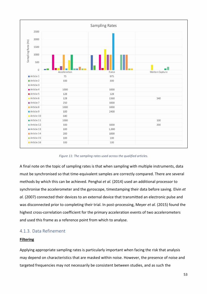
53
Figure 11: The sampling rates used across the qualified articles.
A final note on the topic of sampling rates is that when sampling with multiple instruments, data
must be synchronised so that time-equivalent samples are correctly compared. There are several
methods by which this can be achieved. Penghai et al. (2014) used an additional processor to
synchronise the accelerometer and the gyroscope, timestamping their data before saving. Elvin et
al. (2007) connected their devices to an external device that transmitted an electronic pulse and
was disconnected prior to completing their trial. In post-processing, Meyer et al. (2015) found the
highest cross-correlation coefficient for the primary acceleration events of two accelerometers
and used this frame as a reference point from which to analyse.
4.1.3. Data Refinement
Filtering
Applying appropriate sampling rates is particularly important when facing the risk that analysis
may depend on characteristics that are masked within noise. However, the presence of noise and
targeted frequencies may not necessarily be consistent between studies, and as such the

54
recommended filters may not be directly transferable. Although these rates may be different
between studies and applications, understanding the spectrums and filters used in other studies
may indicate areas of the spectrum for further consideration in future design planning, and as
such their methods shall be considered. Within this, one must consider that whilst the eliminating
noise is important, there may be particular frequencies that are helpful for modelling the
respective parameters. 36F
37 Different kinds of movements and landings contain different frequency
makeups: “the appropriate cut-off frequency depends on the frequency content of the signal,
which in turn depends on the type of task performed” (Simons and Bradshaw, 2016). As shown
earlier, primary frequencies within the signal may be sufficient to model the waveform of a
runner.
Using a frequency histogram, Penghai et al. (2014) determined that in their jumping trial, targeted
frequencies at the trunk were between 0 to 30 Hz, and they as such used a lowpass filter at 30 Hz.
Zhang et al. (2008) observed that in drop landings, within the 100 ms after initial foot contact, the
first and second peak power of tibial accelerations was between 21 to 50 Hz. In a running trial,
Lafortune et al. (1995) found that frequencies in the lower leg were greater than 30 Hz. In an
earlier study, Hennig and Lafortune (1991) observed that “a power spectrum analysis of the force
and acceleration signals revealed that more than 99% of the signal's power was below 60 Hz,”
leading them to use a 60 Hz lowpass filter. They later found that 98% of this content was below
100 Hz (Lafortune et al., 1995). However, contrary to this, Antonsson and Mann (1985) found that
in walking, 99% was contained under 15 Hz. These results clearly differ between activities and
locations, but it seems that there is a consistent gait signal content below 100 Hz.
Correlation strength has been found to differ between use of different filters. When comparing
locations across the back, Simons and Bradshaw (2016) found that a 20 Hz filter on the upper back
produced the overall best correlations between PRA and GRF. Wundersitz et al. (2013) found that
for the most appropriate indirect measure of peak GRF, 8 to 10 Hz was best for walking and
running tasks, suggesting that resultant acceleration data be smoothed with a 10 Hz filter.37F
38 In a
later study, they again found that these filters significantly reduced errors between raw and actual
acceleration data (Wundersitz et al., 2015). Rantalainen et al. (2018) also considered the effects of
filtering acceleration data from the upper back, with low-pass cut-offs between 6 Hz to 20 Hz.
37 Chapter 3.1, Recording at the Lower Limb. 38 It is important to note that this was a smoothing of the resultant acceleration data; not the uniaxial data.

55
However, they found that filtering had very limited effect on acceleration error and chose to
therefore apply no filter.
Error Reduction
Another consideration for force recording is that a recording threshold may need to be
determined, above which the input data is deemed valid. Jiang et al. (2019) considered the gait
cycle to have started when force was above 0 N; Hennig and Lafortune (1991) considered foot
contact as above 5 N; Guo et al. (2017) above 10 N; Pieper et al. (2020) above 20 N. Havens et al.
(2018) considered peak vertical GRF to occur at the first peak following 30 N of contact. The
inclusion of these thresholds can reduce errors: Udofa et al. (2016) attributed their over-
prediction of force to having not incorporated a 40 N contact-identification threshold. They further
showed how this can impact impulse predictions, saying that the “inclusion of the threshold setting
at the beginning and end points of the impulse curve function with preservation of the
mathematical area under the curve would lower the peak value.” They said that ultimately, the
main error was more likely due to the lack of a threshold than the shape of their sine function.
Accelerometers, gyroscopes and magnetometers can provide information on orientation for gait
analysis in space without motion capture systems (Mundt et al., 2020). However, this is not
without limitation, since accelerometers and gyroscopes are susceptible to drift and noise that can
cause error accumulation in multi-step analyses; this is also a problem when testing over long
periods (Tao et al., 2007). Magnetometers “…are highly susceptible to local disturbances in the
magnetic field” (Mundt et al., 2020). Systematic biases have been found in commercial
accelerometers of between 0.46 g and 1.39 g, with biases increasing with higher loadings (Meyer
et al., 2015). The sensitivity of accelerometers to linear accelerations, and the drift and inclination
direction of gyroscopes, have been raised as concerns in sensor design (Abdelhady et al., 2019). It
has been suggested that accelerometer bias may corrected by establishing a regression model
(Meyer et al., 2015). Gyroscope drift may be correctable by resetting the system after each gait
cycle and by highpass filtering (Tong and Granat, 1999). Takeda et al. (2009) applied a highpass
filter to the raw angular velocity data to remove noise prior to integrating their data for
determining joint angles, minimising drift error from raw integration.
4.1.4. Result Validation
Whether or not these relationships can be determined consistently, validity must be determined
objectively. As such, the performance of these algorithms and which methods should be chosen

56
for data analysis must be set. This review does not aim to address methods for statistical analysis
in sports medicine and exercise science,39 but it will consider some noteworthy tools used in
previous studies. Studies have used tools such as direct correlations, Bland-Altman plots (Raper et
al., 2018) and one-dimensional statistical parametric mapping (Callaghan et al., 2018) to compare
acceleration and force data.
Methods of comparative analysis include determining the closeness of a prediction model by
testing it with the data of a participant from whom the model was not trained. When Lafortune et
al. (1995) tested their Fourier waveform models, they developed individual-participant models
and multiple-participant models, testing these against the participant(s) who had not been
included. They found that where the individualised algorithms produced mean standard deviations
of 𝑀𝑆𝐷 = 0.11 to 1.10 across the five participants, the generalised algorithm, which was
developed from four and tested against the fifth, led to larger deviations of 𝑀𝑆𝐷 = 0.26 to 1.26.
Tan et al. (2020) similarly developed a 14-participant model, testing against the 15th participant.
Guo et al. (2017), rather than dividing their data by participants, halved the data of all participants
and tested their model with the remaining 50% of the dataset. Both Tan et al. (2020) and Guo et
al. (2017) obtained almost perfect results (𝑟 > 0.90) with their machine-learning-based models,
showing that a generalised algorithm could be successfully implemented. In a slightly different
context,40 Mahdavian et al. (2019) considered several different machine learning strategies where,
along with speed and angular velocities, they included the weight and height of 108 participants as
inputs to train the algorithm. When testing against two participants, their results demonstrated
strong correlations (𝑅 = 0.89 to 0.97) in the forces and moments of all three axes.
When considering acceptable rates of accuracy, Tran et al. (2012) set the limit of acceptability to
20%, justifying this by explaining that “though it is acknowledged that CV values above 10% are
rejected in other fields of research, it has been proposed that this analytical goal is often selected
as an arbitrary limit for acceptable variability.” Raper et al. (2018) used a relative measure to
determine the validity of ViPerform, stating that a single calculated stride value would be deemed
invalid “if its value was outside a 20% range of the preceding and following strides,” having
calculated this by “dividing the number of error-free [strides]… by the number of overall strides.”
39 This information can be reviewed in Hopkins et al. (2009) and Bernards et al. (2017). 40 Mahdavian et al. (2019) did not primarily investigate acceleration in their models, but also included walking speed and several angular features; the article was excluded because this project primarily investigated the feasibility of acceleration alone.
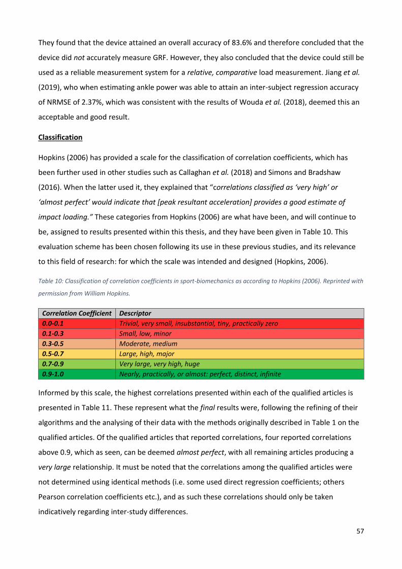
57
They found that the device attained an overall accuracy of 83.6% and therefore concluded that the
device did not accurately measure GRF. However, they also concluded that the device could still be
used as a reliable measurement system for a relative, comparative load measurement. Jiang et al.
(2019), who when estimating ankle power was able to attain an inter-subject regression accuracy
of NRMSE of 2.37%, which was consistent with the results of Wouda et al. (2018), deemed this an
acceptable and good result.
Classification
Hopkins (2006) has provided a scale for the classification of correlation coefficients, which has
been further used in other studies such as Callaghan et al. (2018) and Simons and Bradshaw
(2016). When the latter used it, they explained that “correlations classified as ‘very high’ or
‘almost perfect’ would indicate that [peak resultant acceleration] provides a good estimate of
impact loading.” These categories from Hopkins (2006) are what have been, and will continue to
be, assigned to results presented within this thesis, and they have been given in Table 10. This
evaluation scheme has been chosen following its use in these previous studies, and its relevance
to this field of research: for which the scale was intended and designed (Hopkins, 2006).
Table 10: Classification of correlation coefficients in sport-biomechanics as according to Hopkins (2006). Reprinted with
permission from William Hopkins.
Correlation Coefficient Descriptor
0.0-0.1 Trivial, very small, insubstantial, tiny, practically zero
0.1-0.3 Small, low, minor
0.3-0.5 Moderate, medium
0.5-0.7 Large, high, major
0.7-0.9 Very large, very high, huge
0.9-1.0 Nearly, practically, or almost: perfect, distinct, infinite
Informed by this scale, the highest correlations presented within each of the qualified articles is
presented in Table 11. These represent what the final results were, following the refining of their
algorithms and the analysing of their data with the methods originally described in Table 1 on the
qualified articles. Of the qualified articles that reported correlations, four reported correlations
above 0.9, which as seen, can be deemed almost perfect, with all remaining articles producing a
very large relationship. It must be noted that the correlations among the qualified articles were
not determined using identical methods (i.e. some used direct regression coefficients; others
Pearson correlation coefficients etc.), and as such these correlations should only be taken
indicatively regarding inter-study differences.

58
Table 11: The best correlations between acceleration and GRF as presented within each of the qualified articles.
Classification Study Best Correlation Classification Study Best Correlation
Almost Perfect [5] 0.993 Very Good [12] 0.877
[2] 0.95 [13] 0.86
[14] 0.94 [1] 0.832
[9] 0.9 [3] 0.82*
[4] 0.812
[7] 0.76
[16] 0.76*
[11] 0.71
Not Reported [6], [8], [10] [15] 0.7*
*this article also presented only moderate correlations

59
Chapter 5. Applying the Relationship
Research Aim #3
Determine whether this relationship is generalisable between subjects,
movements, and external conditions.
Research Aim #4
Determine whether measuring acceleration at the lower limb using wearable
accelerometers can provide data that is useful for the prevention or monitoring
of injuries, fatigue, and rehabilitation.
5.1. Difficulties in Model Generalisation
In the previous chapters, it has been shown that an identifiable relationship between acceleration
exists within the body, and it can be determined at the lower leg. However, these models clearly
differ between the kind of movements that are trialled. As such, in this section, the effects of
movement and technique will be considered. Following this, effects on the relationship of several
inter-personal differences will be considered, including physical ability, movement, and external
conditions.
5.1.1. Activity Differences
There were a variety of activities for which the trials in the qualified articles were conducted.
These have been presented according to activity type in Figure 12, with activities being grouped
based on similar movements. If a wholistic, efficacious model is to be developed for a generalised
population, the effects of different movements on these models must be understood and, if
necessary, changes implemented into the algorithms accordingly.

60
Figure 12: Sports used in the qualified articles. Activities have been grouped according to similarity.41
When considering these activities in light of the correlation results that have been presented, the
highest three correlations (0.94 to 0.99) were produced in trials where participants had either
walked or ran. However, to immediately say therefore that these activities are the best for
determining any relationship may not be accurate, since the fourth highest correlation (0.9) was
produced in the only study that pooled results from a variety of activities (Meyer et al., 2015). In
fact, whereas the highest result was observed in a study that considered walking (Guo et al.,
2017), the second lowest of the results came from the other study that considered walking (0.7)
(Pieper et al., 2020). In light of the previous discussion, perhaps the kind of modelling used was
the primary reason these studies produced different results. For example, Guo et al. (2017)
considered machine learning, whereas Pieper et al. (2020) considered direct linear correlations.
However, studies which have focussed on walking alone have been critiqued in the literature, with
the claim that “investigating only walking leads to overestimation of sensor accuracy due to the
fact that the passive dynamics of walking lead to stereotypical patterns that are easier to predict”
(Jacobs and Ferris, 2015). As such, the present accuracy of these studies should not be considered
as generalisable for all activities. Every article that considered jumping produced correlations of
less than 0.9, which may indicate that the ground reaction force waveform during jumping is less
conformed to a single pattern; or at least not as easily predicted from. Nevertheless, even these
correlations would still be classified as very large, and as such should not be disregarded; for,
41 Although pace bowling could be considered running, due to the unique nature of the plantar action of the foot and the rotation of the trunk during a delivery (Callaghan et al., 2018), the running-movement from Article [1] has been kept separate.

61
besides modelling algorithms, there may be physiological factors which are much more indicative
of any such relationship. The differences present between individuals in movement performance
will be further considered in the following section.
Trial Design
The importance, and also a clear a limitation, of cyclic-only studies is seen in that “studies on
wearable sensors that only investigate overground and treadmill walking do not deal with the
amount of variability that happens in daily life” (Jacobs and Ferris, 2015). Having noticed this,
Meyer et al. (2015) attempted to develop a force prediction model from the accelerations of
various activities, including one step each from each trial of six different kinds of activities. Despite
their accelerometers holding systematic bias, they obtained linear correlations of 0.90. The trials
included within this study are shown in Figure 13. This would confirm the conclusion that the
investigation of non-stereotypical tasks can lead to more accurate assessments with these kinds of
technologies. Jacobs and Ferris (2015) have further explained that “not including swing phase data
in estimation also reduces variability in the data set because it assumes that non-linear transition
between stance and swing is predicted perfectly despite sensor noise.”
Figure 13: The activities trialled within the study from Meyer et al. (2015). Reprinted with Permission from Taylor &
Francis.
Netball
Within this discussion on the movement-based effects of force modelling, as has been mentioned,
the end purpose of any device must be considered within the trials for which it is designed. The
context of this thesis is an investigation into the movements within the team sport netball, and as
such the eminent movements performed by players during a netball match should be of primary
concern within the future development of this project. Netball Australia (2016) has explained the

62
key skills and movements involved in the footwork of players during a game. Summarised below,
these movements include stance, coordination, footwork, and balance:
- The two-foot landing controls the hip and knee, where during landing, the knee and toes
are kept aligned, and the knee is kept slightly bent. Younger players may step forward with
one point to maintain balance when lacking core strength required to maintain the stance.
- The one-foot landing depends on the player’s leading direction: leading in the right results
in the player landing on their right foot; leading to the left results in landing on the left.
Players keep their body weight over the outside foot, with shoulders evenly distributed
over the foot; the second foot is planted quickly following this. The player must bend at the
hips, knees, and ankles to cushion their landing.
- Take-off involves starting with smaller steps and strides, quickly moving to larger steps.
When leading to the right foot, a player should take off with the right foot; when leading to
the left, they take off with the left foot.
- The two-foot jump involves bending slightly at the hips, knees, and ankles with the weight
of the player distributed over knees and toes. The player steps into take-off with the left-
right or right-left step pattern and uses both arms to reach and extend upwards. Players
land on both feet and cushion their landing by bending at the knees, hips, and ankles.
Younger players may be instructed to keep their feet shoulder width apart.
- The one-foot leap involves players, when running at an angle to the thrower, bend at the
hips, knees, and ankles, and run with their weight forward over the toes, pushing off from
the take-off foot. The player lands on their outside foot, cushioning by bending at the hips,
knees, and ankles.
- A pivot (outside turn) continues natural body movement after a player has received the
ball at full stretch, pivoting on the landing foot. Their weight is brought over the landing
foot before turning on the ball of the foot and pushing off with the other foot.
Several of these movements are further specified within 9.6 Footwork of the netball rule book
(International Netball Federation, 2020).
5.1.2. Personal Factors
Technique
Factoring intra-personal characteristics into this study on kinetics, it has been identified that “the
ability to accelerate can be effected by an individual’s sprinting technique, force production

63
capability, and the ability to apply that force in the horizontal direction” (Macadam et al., 2017). In
light of such ability-effected differences, it is expected that understanding these differences in
technique would be a primary concern in the development of any kinetically driven model.
However, apart from foot-strike patterns, which will be considered below, none of the qualified
articles specifically targeted understanding the differences of technique when developing the
force-acceleration relationship. Trial inclusion criteria within the studies included being elite or
sub-elite triathletes (Raper et al., 2018),42 adults with regular participation in competitive sport
(Wundersitz et al., 2013),43 and moderately active children (Meyer et al., 2015).44 All studies
excluded people with recent injuries, except Havens et al. (2018), who recruited only participants
that had undergone ACL reconstructive surgery within six months prior to the trial. Since results
from elite participants may not necessarily be true also for amateur participants, this may be an
important research area in future study.
Davis et al. (2018) studied the differences between strike patterns across 169 participants. They
found that vertical average loading rate had larger correlations with vertical tibial acceleration in
runners with front-foot-strike (FFS) (𝑟 = 0.82) than rear-foot-strike (RFS) (𝑟 = 0.66). Summarising
several sources in the literature, Futrell et al. (2020) found that “the load rates associated with a
habitual FFS pattern are approximately 35%–45% lower than that of a habitual RFS pattern.
Transition to an FFS pattern has been associated with a 35%–65% reduction in vertical load rates.”
Following up on this, they furthermore found that this transition reduces load rates more than
altering the cadence of a runner (Futrell et al., 2020). Although cadence does not typically change
foot strike technique (Futrell et al., 2020), research has shown that when running, increasing
cadence by 8.6% can reduce average vertical load rates by 18.6% (Willy et al., 2016).
In addition to technique, natural movement can also cause errors, with high trunk rotation of the
accelerometer during the moment of recording being found to skew results (Callaghan et al.,
2018). Wundersitz et al. (2013) has also observed that during running, as the severity of the
change of direction increases, the correlation between the acceleration and GRF decreases: their
prediction variance from change-of-direction tasks (24%) was double that of straight line running
(12%). This may have been in part due to the presence of a technology bias, since Meyer et al.
(2015) had found that measurement bias was found to increase with higher loadings; that is, with
42 Elite and sub-elite was defined as anyone “who trains regularly with a coach and has a specific training/competition aim” (Raper et al., 2018). 43 Defined as one or more events per week. 44 Defined as less than three hours of weekly exercise outside regular school activities.

64
higher loadings, the degree of overestimation of the accelerometers against the force plate
increased. These errors and movement-varying measurements surely present a case for the
inclusion of multiple movements within any trial development, since any device developed must
be equipped to compensate for the wide range of movements that can be expected in any
situation.
Impairment
However, physical differences between participants are not only limited to the size, mass, or
strength of a person, but also extends to their physical ability; technique is influenced not only by
skill and prior training, but also by impairment. In a comparison of healthy patients with those
impaired by multiple-sclerosis, Alaqtash et al. (2011) established a reference rule-base from
unimpaired subjects, from which to compare the gait force and acceleration to those with MS.45
The fuzzy-algorithm comparison identified distinctions in gait waveforms between patient sets.
For example, the contact force of MS patients was flat with a single peak, with patients having a
significantly longer stance phase.
There was only a moderate similarity within the loading response gait phase between patient sets,
with force similarities of 0.634 (Y-axis) and 0.659 (Z-axis). Grades of similarity between swing
phases were particularly low, with an average phase similarity of 0.179 (initial swing), 0.008 (mid-
swing), and 0.289 (terminal swing). These differences were attributed to the abnormal muscle
activities within the tibialis anterior, quadriceps and gluteus medius of MS patients, further
observing that “the acceleration curves of the thigh and the hip… [demonstrated low] accelerations
for MS compared to healthy subjects throughout most of the gait phases” (Alaqtash et al., 2011).
There was a sharp increased acceleration at the initial contact phase of the MS gait cycle, and
insufficient foot clearance during initial swing phase, which will further complicate distinctions in
identifying waveform events and in using these to predict force based on a generalised model.
5.1.3. External Factors
Footwear and Landing Surfaces
Within the development of these algorithms and testing procedures, one must consider not only
inter- and intra-personal differences, but also where each activity has been conducted. For
example, with regards to outdoor sprinting, wind resistance is a crucial factor to consider,
45 Alaqtash et al. (2011) did not predict force from acceleration, but only compared the gait parameters between impaired and unimpaired subjects.

65
especially with such conditions being conducive to fatigue (Hunter et al., 2005). These fatigue-
induced effects on running mechanics must be measured in external settings, rather than only the
laboratory, since “in order to get insight into the specific challenges runners face outside the
laboratory in real world, measurements need to be performed outside the laboratory in a setting
as specific as possible” (Reenalda et al., 2016). Although external tests may not be possible in
initial development stages when force plate-based validation is necessary, this kind of trial may be
completed by using pressure insoles.
Rouhani et al. (2014) was able to use pressure insoles for estimating gait dynamics by first
calibrating their pressure insoles with laboratory force plates, and then developing a pressure
distribution map based on those initial measurements. This calibrated insole pressure map was
used to estimate force and torque outside the laboratory, obtaining a coefficient of multiple
correlations above 0.90. If high accuracy can be obtained consistently, then technology such as
this could be used to validate external accelerometer-based force predictions.
Incorporating the differences of external factors into the development of a prediction model may
also be important for its reproducibility since landing surfaces and shoe stiffnesses have been
found to influence landing impact dynamics. When comparing the effect of shoe compliancy on
impact kinetics, Bruce et al. (2019) found that greater shoe compliance resulted in lower peak
resultant tibial acceleration (𝑝 = 0.005), but that peak vertical GRF was not different between
landing surfaces and shoe types (𝑝 ≥ 0.056). However, when considering soft and stiff landing
surfaces, Devita and Skelly (1992) obtained the results in Figure 14. They found that although the
temporal features of the waveform were similar between surfaces, landing on a stiff surface had a
23% larger impulse than on a soft surface.

66
Figure 14: Comparison of ground reaction force between soft and stiff surfaces (Devita and Skelly, 1992). Reprinted
with permission from Wolters Kluwer Health, Inc.
Tan et al. (2020) considered different kinds of footwear, foot strike patterns, step rate, and
running speeds, and they found that their convolutional neural network did not generate
significantly different results.46 They did find that wearing minimalistic footwear had a higher
correlation coefficient (0.95) than standard footwear (0.88), which may indicate that standard
footwear absorbed more of the force upon impact. Furthermore, peak positive acceleration has
been reported to reduce by between 11-20% between different shoes (Crowell and Davis, 2011).
Future studies may benefit from including information on shoe compliance when predicting
impact. However, it has been said recently that evidence for the effect of landing surfaces and
shoe stiffness on jump landing dynamics remains limited (Bruce et al., 2019), and as such, this may
require further investigation.
5.2. Injuries
In the research aims, it was stated that a wearable accelerometer will be considered useful if it is
able to provide information that can be used in the prevention or monitoring of injuries, fatigue,
and rehabilitation. This section will, broadly speaking, seek to establish how some of the
information within this thesis may contribute to an understanding of injury prevention and
management in sport, and the immediate applications of the methods and results that have been
presented within the literature.
46 The results from Tan et al. (2020) can be seen in Chapter 3.2.3, Table 3. Study details: footwear: standard running shoes (Revolution 4, Nike) and minimalist shoes (V-RUN, Vibram Corp); foot strike patterns: FFS, MFS and RFS; step rate: baseline rate, 90% and 110%; running speed: 2.4𝑚𝑠−1 and 2.8𝑚𝑠−1.
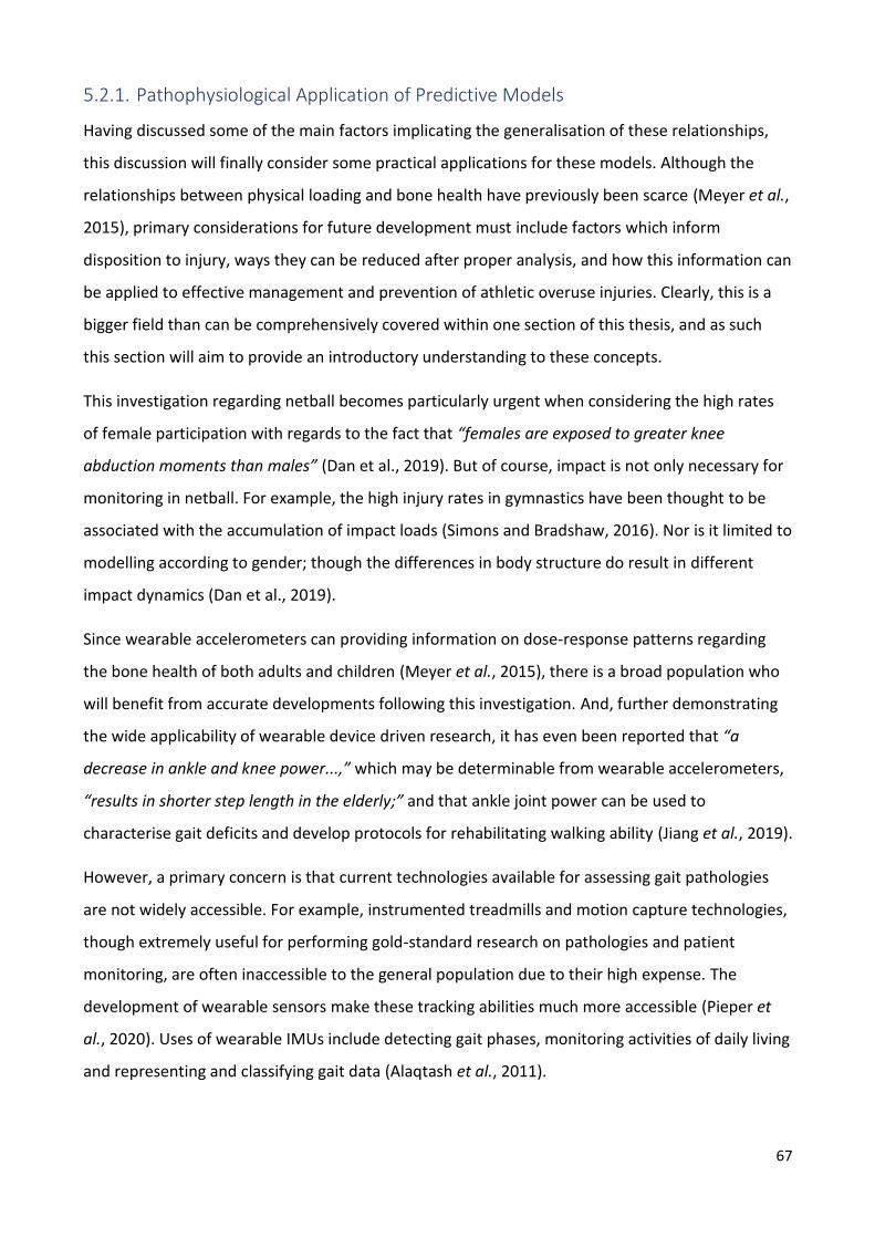
67
5.2.1. Pathophysiological Application of Predictive Models
Having discussed some of the main factors implicating the generalisation of these relationships,
this discussion will finally consider some practical applications for these models. Although the
relationships between physical loading and bone health have previously been scarce (Meyer et al.,
2015), primary considerations for future development must include factors which inform
disposition to injury, ways they can be reduced after proper analysis, and how this information can
be applied to effective management and prevention of athletic overuse injuries. Clearly, this is a
bigger field than can be comprehensively covered within one section of this thesis, and as such
this section will aim to provide an introductory understanding to these concepts.
This investigation regarding netball becomes particularly urgent when considering the high rates
of female participation with regards to the fact that “females are exposed to greater knee
abduction moments than males” (Dan et al., 2019). But of course, impact is not only necessary for
monitoring in netball. For example, the high injury rates in gymnastics have been thought to be
associated with the accumulation of impact loads (Simons and Bradshaw, 2016). Nor is it limited to
modelling according to gender; though the differences in body structure do result in different
impact dynamics (Dan et al., 2019).
Since wearable accelerometers can providing information on dose-response patterns regarding
the bone health of both adults and children (Meyer et al., 2015), there is a broad population who
will benefit from accurate developments following this investigation. And, further demonstrating
the wide applicability of wearable device driven research, it has even been reported that “a
decrease in ankle and knee power...,” which may be determinable from wearable accelerometers,
“results in shorter step length in the elderly;” and that ankle joint power can be used to
characterise gait deficits and develop protocols for rehabilitating walking ability (Jiang et al., 2019).
However, a primary concern is that current technologies available for assessing gait pathologies
are not widely accessible. For example, instrumented treadmills and motion capture technologies,
though extremely useful for performing gold-standard research on pathologies and patient
monitoring, are often inaccessible to the general population due to their high expense. The
development of wearable sensors make these tracking abilities much more accessible (Pieper et
al., 2020). Uses of wearable IMUs include detecting gait phases, monitoring activities of daily living
and representing and classifying gait data (Alaqtash et al., 2011).

68
IMUs can be used to differentiate between walking, running, and jumping locomotion, and to
distinguish between different intensities (Lee et al., 2015). Meyer et al. (2015) has commented
that “accelerometers are perfectly suited to measure impact loading of bone,” and Pieper et al.
(2020) has stated that when using shank acceleration to study the effects of knee bracing and its
significance for aiding in the rehabilitation of those with trailing limb propulsion, “shank
acceleration may effectively distinguish intrasubject variations over time, for example due to
functional decline or clinical rehabilitation.” Indeed, using low cost, simple sensors may allow the
identification of abnormal gait patterns such that falls can be prevented in the older population,
prolonging the time with which they can retain independent mobility (Mundt et al., 2020).
Load Accumulation
Using wearable devices to predict impact dose will enable an objective quantification of loading,
rather than relying on subjective ratings of perceived exertion. The effects of ACL reconstruction,
which alter a client’s lower extremity mechanics, are seen weeks and years after surgery (Havens
et al., 2018), which makes long-term, subjective assessments consistent. This objective rate is
what is of primary interest in this study, since “the aetiology of overuse injuries appears to be
related to both the impact and peak forces the limbs experience during each loading cycle” (Udofa
et al., 2016). Accelerometers have previously been used in representing player load by measuring
accumulated impact forces over time (Wundersitz et al., 2013). Alternatively, Tan et al. (2020)
considered the possibility for loading rate to contribute to these models. They concluded that
machine-learning-based vertical average loading rate “could enable runners to more accurately
assess impact loading rates and potentially provide insights into running-related injury risk and
prevention” (Tan et al., 2020).
Clearly, the development of any objective analysis for injury risk will require a consistently
accurate risk function that uses kinetics to predict overuse injury. Bailey et al. (2018), who
considered the modelling of risk in light of the shorter duration high impact loading from military
injuries, developed an injury risk function based on the results of axial loading to post-mortem
human legs. In their conclusions, they estimated that there was “50% risk of injury for a leg
exposed to 13 Ns of impulse at peak force and 8.07 kN of force for force durations less than and
greater than half the natural period of the leg, respectively” (Bailey et al., 2018).
Similar to how Bailey et al. (2018) quantified risk in terms of impulse, Winter (2005) has explained
that “integration of the force–time history [i.e. impulse] can be used to provide a velocity–time

69
profile of the body’s center of mass and so provide a basis for calculations of the products of force
and velocity.” Taking this backwards, if integration of the acceleration waveform could be used to
estimate impulse (the integration of the force waveform), then perhaps a risk factor could be
given based on integration of acceleration alone, without needing to focus on event-to-event
predictive force modelling. If developed for the purpose of predicting overuse injury risk, these
functions will enable a translation of repetitive axial loading into a demonstration of injury
prediction.
The kind of short term risk analysis that Bailey et al. (2018) has presented may even be indicative
of the short-term, high impacts experienced during athletic sports. However, further research into
objective quantities of player load must first be made more widely accessible, since when lacking
this, previous research has turned to acceleration-based arbitrary loading units to measure player
load (Bailey et al., 2017),47 which do not necessarily translate into known quantities.
This understanding of player loading may not be limited only to injury prediction and prevention
but may also extend to using this technology for protective purposes (Gabbett and Ullah, 2012).
Indeed, “although excessive training loads may increase intrinsic injury risk, insufficient loads may
achieve the same outcome, with a certain level of load (in-between an underload and overload)
likely to be protective for injury” (Colby et al., 2014). Providing players with a minimum loading
dose is even necessary for bone and musculoskeletal tissue health, but must be carefully
administered, lest higher loads lead to overuse injuries (Udofa et al., 2016).
This research is particularly important when considering team sports, where this training “reflects
a balance between the minimum training load required to elicit an improvement in fitness and the
maximum training load tolerable before sustaining marked increases in injury rates” (Gabbett and
Ullah, 2012). Although more could be said on the benefits of protective loading levels, the
discussion will now briefly turn to three other pathophysiological benefits that impact modelling
from wearable device-collected kinematics may provide: landing, fatigue, and limb propulsion.
Landing and Fatigue
Although Elvin et al. (2007) found that jump height did not correlate with peak acceleration or
peak force, their initial proposition that jump height may be “an important predictor of ground
reaction force and overuse knee injury,” is yet to be disproved. However, if this is so, then the
47 Bailey et al. (2017) is not the same author as Bailey et al. (2018).

70
variables must be related. The idea of impact dose for injury prevention and shock attenuation
without considering ground reaction forces may not be suitable, since this study seems to suggest
that shock reduction does not significantly improve with elevated mechanical demands (Zhang et
al., 2008). In fact, landing height has been found to have no significant effect on acceleration
during impact (Zhang et al., 2008), which may justify the earlier proposition that jumping events
are more difficult to estimate force from acceleration than running events are.48 More recently,
Gokeler et al. (2017) has demonstrated how accelerometers can be used as rehabilitative
assessments before returning to activities post ACL reconstruction by assessing jump height and
power.
Coventry et al. (2006) found that following a jumping protocol, their ten participants were
fatigued, but without significant shock attenuation throughout their body, and Simons and
Bradshaw (2016) summarised these effects by explaining that fatigue results in increased GRF
without substantially changing the acceleration. This complicates the acceleration-force
relationship by implicitly affirming that there are other factors that can lead to increased forces.
However, Reenalda et al. (2016) has reported that fatigue can increase peak acceleration, and that
“an increase in peak acceleration might indicate higher loading rates, a reduction in shock
absorption quality and a higher impact on the body.” They further explained that changes in
running technique over long periods of physical activity may not necessarily be due to fatigue, but
may rather be due to the body adapting its technique to cope with the high impact stresses on the
body (Reenalda et al., 2016).
This is consistent with Coventry et al. (2006), who has also explained that the body can maintain
shock absorption over longer periods of physical exercise by altering its kinematics. This research
seems to indicate that although force, acceleration, and fatigue are interrelated, fatigue may not
be the best indicator of risk, since bodily changes in response to fatigue are apparently not
consistent. However, in netball matches, Best (2017) found a significant association between
match quarter and injury occurrence (𝑝 = 0.019), with peak incidence occurring in the third
quarter, where it is expected that fatigue would be intensifying. This seems to be a necessary area
of future research.
48 Chapter 5.1.1, Differences by Movement.

71
Limb Propulsion
This relationship could also be used for monitoring and predicting the pathologies of trailing limb
propulsion. Pieper et al. (2020) tracked the propulsive force output of healthy participants before
and after inhibiting their movement with a leg brace by diminishing the right limb propulsion of
their participants by simulating a leg impairment similar to that following stroke. Although they
found that the unilateral leg-brace impairment did not replicate the neuromuscular limitations
present following stroke, they found that the knee brace caused a systematic and significant
reduction in limb propulsion: they observed a reduction of the very large correlations in the
uninhibited leg (𝑅2 = 0.77) to very small correlations in the inhibited leg (𝑅2 = 0.31). This
research indicates that propulsive inhibitions could be detectable through accurate gait propulsion
and loading predictions. Such propulsive distinctions have also been trialled by Browne and Franz
(2019), who found that one could monitor the modulation of trailing limb propulsion by tracking
the angular velocities about the ankle.
The technology could be used to monitor technique, looking in advance for signs of oncoming
injury. Lee et al. (2015) has found that acceleration and angular velocity can contribute to
distinguishing between intensity levels, and in particular that angular velocity “can be used to
distinguish between locomotion modes at the same intensity level.” Although angular velocity is
not dependent on force, this does demonstrate that wearable accelerometers are able to provide
information on gait characteristics for the purpose of pathological monitoring. More directly, Dan
et al. (2019) has proposed that using acceleration-predicted ground reaction force, can indeed
enable devices to screen for asymmetrical gait differences between individuals. Of course,
propulsive behaviours are only one aspect of understanding technique modulation post-injury, but
it can be seen that there is potential for broad application of this kind of technology by monitoring
parameters associated with gait impairments.

72
Chapter 6. Future Research Areas
As recommended within the literature .
Research Aim #5
Determine information on the running of a trial such that new data can be
collected, and a relationship derived, based on the recommendations and
performance of these studies.
6.1. Research Implications
Having presented the previous works within the literature, a summary of the future research areas
that were recommended in the qualified articles will be given. These recommendations will be used
to design a validation trial, wherein the literature-based conclusions and the data of a previous
trial will be revaluated in light of the strategies discussed. The summaries within this chapter are
only the primary areas for future research that were raised in the qualified articles and are not
exhaustive for areas of literature-warranted future research. It may be noted that some of the
raised research areas have already been briefly covered within the review; these are included for
the purpose of relaying the primary areas that were raised within the articles as future needs.
6.1.1. Recommendations
Future research should determine optimal placement sites for wearable accelerometers,
accounting for the reasons of each and considering strengths of using information from multiple
locations (Havens et al., 2018, Pieper et al., 2020, Tan et al., 2020, Tran et al., 2012, Wundersitz et
al., 2013). It should aim to understand the degree to which movement artefact and soft tissue
attenuation at each position affect results (Callaghan et al., 2018, Havens et al., 2018). Attachment
methods should be designed for securing against this movement artefact between people, limiting
device vibration and movement (Tran et al., 2012, Wundersitz et al., 2013). Interpersonal
differences in landing and movement technique should be accounted for, especially with regards
to how technique may change over time (Simons and Bradshaw, 2016). This may involve further
understanding the contribution of joint angles to peak forces, accelerations, and impact
attenuation (Elvin et al., 2007, Simons and Bradshaw, 2016, Tran et al., 2012).
Signals may need to be corrected for gravity and the effects of contact angle when calculating the
vertical force componentry (Hennig and Lafortune, 1991). Naturally, this may contribute towards

73
the need for modelling the shock attenuation of lower limb kinematics and how it affects force
and power (Lafortune et al., 1995). This may involve including considerations for landing surfaces
(Simons and Bradshaw, 2016) and footwear (Tan et al., 2020).
Further research is required to confirm logarithmic force-acceleration model correlations (Charry
et al., 2013). All models should be validated for accurate prediction and for activities of daily living,
particularly those which have been designed with machine learning (Guo et al., 2017, Lafortune et
al., 1995). Force approximation models should be mapped to specific gait events, and specifically
should determine whether the maximum projection of the relationship occurs at mid-stance,
when the leg is geometrically perpendicular to the ground (Charry et al., 2013). The development
of these models that relate GRF with PRA should include factoring in the effects of body weight,
and may mean developing personalised algorithms (Raper et al., 2018, Simons and Bradshaw,
2016).
This research will need to confirm whether vertical tibial acceleration is indeed the best surrogate
for load rate in runners (Davis et al., 2018), and contribute to further understanding the value of
segment acceleration in the athletic movements of a wider variety of sports, including for pace
bowling performance (Callaghan et al., 2018, Elvin et al., 2007) and for machine learning
developments (Tan et al., 2020). Running load impairment predictors should be identified for
application with knee joint injuries and in rehabilitation protocols like ACL reconstruction (Elvin et
al., 2007, Havens et al., 2018). These predictors should consider a method of determining lower
extremity loads in pre- and post-intervention programs (Raper et al., 2018). Especially regarding
monitoring to pre-injury load levels, consideration should be made for whether prediction models
can be used as relative measurements of load (Raper et al., 2018).
Future research may include the development of technology that identifies gait events outside of
the laboratory (Pieper et al., 2020), with models that simultaneously estimate average,
instantaneous and peak impact load rates (Tan et al., 2020). This software should be further
applied to wider sporting applications and for regular consumer activities, with provisions for
determining leap ability and explosive power (Penghai et al., 2014). The necessity for device
calibration must be established, and additional technologies such as motion capture analysis
should be used for measuring and validating predicted kinematics (Callaghan et al., 2018,
Wundersitz et al., 2013). Devices should be made so as not to interfere with body movement
(Hennig and Lafortune, 1991).

74
Future device development should use triaxial accelerometers as opposed to a single axial so that
multiaxial correlations can be made (Elvin et al., 2007). Dynamic ranges should be selected such
that gravitational accelerations during movement do not extend the limitations of the device
(Meyer et al., 2015). Methods for synchronising motion capture data with device sensors may
need to be considered if additional validation technologies will be considered (Havens et al.,
2018). Frequency analysis should be performed by spectral and wavelet analysis so that high
frequency signal components can be detected and accounted for, especially with regards to
eliminating noise whist retaining signals and in frequency-dependent waveform prediction models
(Lafortune et al., 1995, Wundersitz et al., 2013).
These acceleration frequency components should also be considered for how they differ between
locations like the upper back (Simons and Bradshaw, 2016). Low frequency studies should also be
performed: it needs to be determined whether acceleration cut off frequencies between 20 to 50
Hz are more effective than at 20 Hz (Simons and Bradshaw, 2016). Furthermore, the conclusion
needs to be validated that peak resultant acceleration filtering which maximises correlations is
more important than identifying direct force-acceleration agreements (Simons and Bradshaw,
2016). It must also be determined whether a regression model can negate internal device biases
(Meyer et al., 2015), and validation is required for any device that claims to make accurate
predictions (Raper et al., 2018).
Finally, regarding trial design for the testing of these models, future trials should include a wider
variety of sport-related movements than only jumping and landing, including testing for several
running speed variations and their validity during change of direction tasks (Charry et al., 2013,
Raper et al., 2018, Tran et al., 2012). Trials should be designed for more participants (Charry et al.,
2013, Tan et al., 2020), and the results of previous trials should be extrapolated to larger
populations with elite athletes (Elvin et al., 2007). Trials that have developed models for
participants with previous impairments should be tested for generalisability to non-injured
populations (Havens et al., 2018). Trials should also consider varied age groups and participants
with pathological gaits, rather than only young, healthy volunteers (Guo et al., 2017, Pieper et al.,
2020). Trials should make considerations for broader populations and with equal gender
distributions (Meyer et al., 2015). The clinical utilisation of devices like ViPerform should be
designed to measure average movements across multiple strides, rather than calculating points
for individual strides to obtain higher accuracy (Raper et al., 2018).

75
6.1.2. Investigation Proposal
Since there remains a need for determining these acceleration-force relationships, it is more
expedient to re-evaluate data from two years ago in light of the presented algorithms, rather than
designing a new investigation. The investigation to follow will investigate several of the areas
recommended above, and it will primarily focus on considering device location. It will consider
acceleration proxies for peak forces, load rates, and impulse, simultaneously estimating these
variables. Relevant frequencies will be determined based on a power analysis, and noise will be
eliminated where possible. The effect of using different filters on correlation accuracy will also be
considered. It will consider linear, logarithmic, and machine learning proxy models. It will consider
body weight and personalised algorithms, and model generalisation between participants. A
comprehensive method will be presented in Chapter 7.

76
Chapter 7. Investigation
7.1. Investigation Outline
Corbo (2018) began this project by undertaking a preliminary trial to consider the initial validity of
the acceleration-force relationship. Participants performed repetitions of up to nine different
activities to simulate the kinds of movements experienced in a netball match. The highest
correlations obtained using linear correlations were 𝑅2 = 0.64, between the integration of vertical
force and axial acceleration (Corbo, 2018). In this chapter, the data that was collected in this trial
will be re-evaluated in light of the findings gained from the literature to determine whether higher
correlations can be obtained.
7.1.1. Background
In the previous study, four participants were instructed to complete nine sets of activities akin to
the movements performed in netball. The instructions that were given to participants have been
summarised in Table 12. In total, there were 111 individual movements completed by the four
participants, but participants did not necessarily complete the same number of repetitions of each
movement. In some movements, both legs of a participant may have been in contact with the
force plates, so where possible, data from both legs was recorded. Across both legs across the 111
trials, there were 135 valid recordings.
Table 12: Instructions given to participants for completion within the study.
Activity Instruction
Walk From a start line, walk towards and over the force plates.
Jog From a start line, run with mild effort over the force plates.
Run From a start line, run with medium effort over the force plates.
Sprint From a start line, run with maximal effort over the force plates.
Cut Sprint towards the force plates. Strike a plate with the dominant foot, then change
running direction 45°, following through on the contralateral foot.
Step-Down Passively step down from a platform of 𝑥 mm height.
Jump Begin by standing with both feet on a single force plate. Using a bilateral arm swing, jump
from a standing position with maximum effort.
Run-On Receive a thrown ball whilst running towards the force plates. Jump into the catch, landing
with the contralateral leg on a force plate. Continue running past the force plates.
Two-Foot
Land
Sprint towards the force plates. Jump off of one foot and land on two feet, landing with at
least one foot on the force plates.
A trial was deemed valid if an entire foot landed within a force plate. The trials had been
previously visually sighted on VICON to confirm to confirm validity. If a foot landed across multiple
force plates, the total movement kinetic was derived by summing the output of each relevant

77
plate. To confirm this validity, trials were further sighted by comparing the acceleration and force
waveform: trials were valid if the recorded movement was distinguishable from times of non-
contact. Trials were considered invalid if they did not contain a complete waveform, or where
there was no clear distinguishable movement. All trials that were marked invalid were excluded
from this analysis. Valid trials are summarised in Table 13.
Table 13: Valid trials, according to movement type, participant, foot, and force plate.
Participant 1 Participant 2 Participant 3 Participant 4
𝑚1 = 63.2291 𝑘𝑔 𝑚2 = 72.6537 𝑘𝑔 𝑚3 = 73.9738 𝑘𝑔 𝑚4 = 82.0994 𝑘𝑔
Female Male Female Male
Movement Foot Force Plate Foot Force Plate Foot Force Plate Foot Force Plate
Walk
R 4 R 3 R 3 L 1
L 1 R 3 L, R 2, 3 L 1
R 3 R 4
Jog
L 2 R 3 & 4 R 4 R 1 & 2
L, R 2, 3 R 3 L 1 & 2 L 1
L 1 & 2 R 3 L 2 L 1 & 2
Run
L 2 L 1 & 2 L 1 L 1 & 2
L 2 L 2 L 1 L 1 & 2
L 2 L 1 & 2
Sprint
L 2 L 1 & 2 L 1 & 2 L 2
L 2 L 1 & 2 L 1 & 2 L 2
L 1 & 2 L 1 L 2
Cut
R 3 R 3 R 3 L 2
R 3 R 3 R 3 L 2
R 3 & 4 R 3 R 3
440mm Step-Down
R, L 2, 1 R 3
R, L 2, 1 R 3
R, L 2, 1 R 3
450mm Step-Down
R 3
R 3
R 3
460mm Step-Down
L 3
L 3
L 3
600mm Step-Down
R 3
R 3
R 3
660mm Step-Down
R, L 2, 1 L 3
R, L 2, 1 L 3
R, L 2, 1 L 3
Jump
L, R 1, 2 L, R 1, 2 L, R 1, 2 R 4
L, R 1, 2 L 1 & 3 L, R 1, 2 R 4
L, R 1, 2 L, R 1, 2 R 4
Run-On
R 4 & 3 L 2 R 4 L, R 2, 3
R 4 L 2 R 4 L, R 2, 3
R 4 L, R 2, 3

78
R 4
Two-Foot Land
L, R 1 & 2, 4 R 3 & 4 L, R 1 & 2, 3 & 4 L 1
R, L 4, 2 & 1 R 4 R 3 L 1
R, L 4, 2 & 1 L, R 1 & 2, 4 R 4 L 1
L, R 2, 4 R 3 & 4
Data Capture
In the trial, four AMTI OR6-7 Multi Component force plates measuring 464 mm (width) by 508 mm
(length) were sampled at 2000 Hz, with axis orientations as illustrated in Figure 15. These were
used in conjunction with VICON motion capture markers. The arrangement of the force plates and
their utilisation with VICON in determining the validity of trials is shown below in Figure 15.
Figure 15: Force plate and motion capture utilisation.
Six TRIGNOTM Wireless System PM-W01 EMG devices were utilised, inside each of which was an
integrated triaxial accelerometer. These sensors were attached to the anterior medial thigh, the
anterior medial shank, and the ankle lateral malleolus.49 The accelerometers had a software-
selectable dynamic range of ± 1.5 g, ± 4 g, ± 6 g, and ± 9 g. The device in this investigation recorded
with a dynamic range of ± 9 g. The device had a DC bandwidth of 50 ± 5 Hz, 20 dB/sec, and a
sampling rate of 148.1 Hz. The six devices, and their attachment positions and axis orientations,
are shown in Figure 16.
49 Participant 1 had an additional four sensors placed on the medial ankle and heel of each leg. However, for consistency with the other participants, these have been excluded from further analysis.
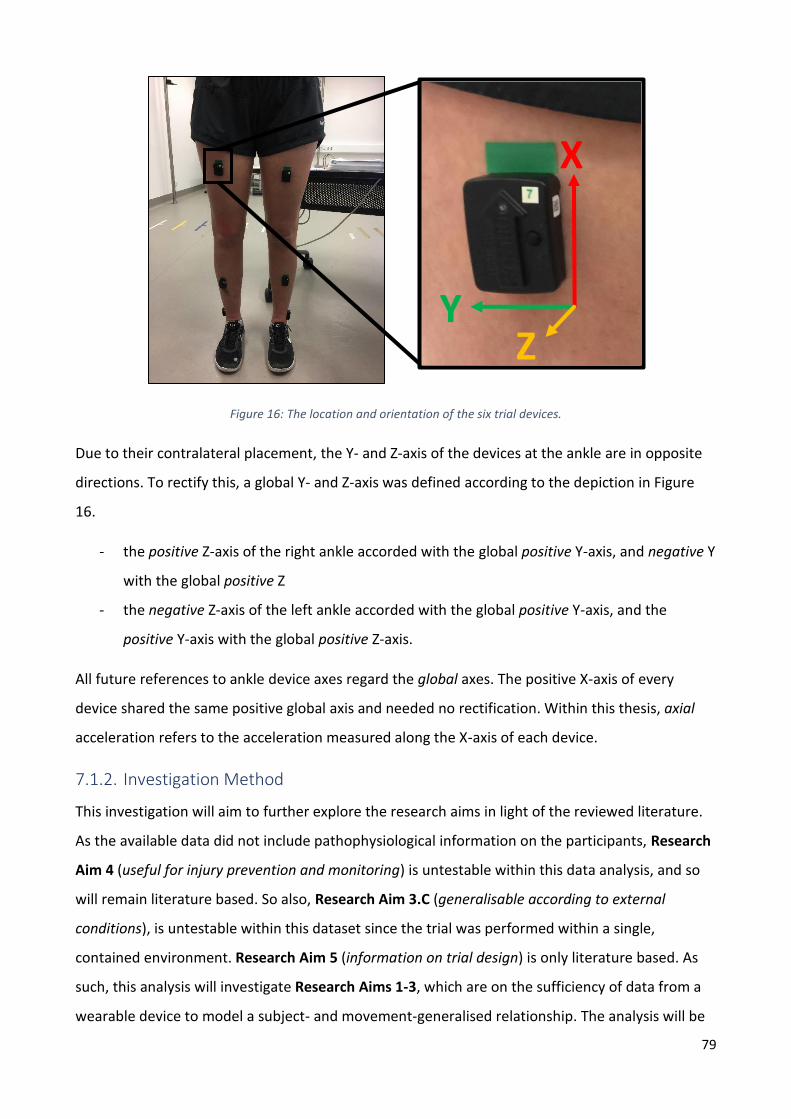
79
Figure 16: The location and orientation of the six trial devices.
Due to their contralateral placement, the Y- and Z-axis of the devices at the ankle are in opposite
directions. To rectify this, a global Y- and Z-axis was defined according to the depiction in Figure
16.
- the positive Z-axis of the right ankle accorded with the global positive Y-axis, and negative Y
with the global positive Z
- the negative Z-axis of the left ankle accorded with the global positive Y-axis, and the
positive Y-axis with the global positive Z-axis.
All future references to ankle device axes regard the global axes. The positive X-axis of every
device shared the same positive global axis and needed no rectification. Within this thesis, axial
acceleration refers to the acceleration measured along the X-axis of each device.
7.1.2. Investigation Method
This investigation will aim to further explore the research aims in light of the reviewed literature.
As the available data did not include pathophysiological information on the participants, Research
Aim 4 (useful for injury prevention and monitoring) is untestable within this data analysis, and so
will remain literature based. So also, Research Aim 3.C (generalisable according to external
conditions), is untestable within this dataset since the trial was performed within a single,
contained environment. Research Aim 5 (information on trial design) is only literature based. As
such, this analysis will investigate Research Aims 1-3, which are on the sufficiency of data from a
wearable device to model a subject- and movement-generalised relationship. The analysis will be
Y
X
Z

80
undertaken in two phases, both of which have been designed with these aims in mind. The
analysis was completed in MATLAB R2020a.
Phase 1: Linear Modelling
Event-to-event correlations will be conducted between the waveforms of each trial, across all
locations and participants.
Before modelling these relationships, noise filters will be applied to the raw kinematic data.
Models will consider both direct linear correlations and mass-scaled linear correlations. Following
this, a 20 Hz filter will furthermore be applied over the acceleration data, in accordance with the
literature-based recommendations,50 to determine the influence of frequency on the acquired
waveforms. Following this, cohort-developed correlations will be validated with a leave-one-out
cross-validation experiment. In this, the acceleration data of three participants will be used to
develop a model that is used to predict the force of the fourth participant; and vice versa, for each
participant.
Phase 2: Non-Linear Modelling
Following the linear modelling of Phase 1, the data will be re-evaluated according to a logarithmic
approach presented in the literature. Rather than determining a new model, the literature model
will be validated with the data of each participant. The correlation coefficients (𝑅2) and the root
mean squared errors (𝑅𝑀𝑆𝐸) of the logarithmic results will be compared to the linear results of
Phase 1.
Finally, a non-linear timeseries machine learning model will be developed for the prediction of the
entire force waveform based on the input acceleration data. The model will be trained with the
data of three participants and validated with the data of the fourth; this will be completed for
each leave-one-out participant combination. The results of the machine learning model will be
compared with the results of the preceding logarithmic and linear investigation.
50 Chapter 6, Future Research Areas.

81
Excluded Models
In addition to the above non-linear models, the literature also presented both a machine learning
event-to-event model and a Fast Fourier Transform waveform model. These have been excluded
from the investigation for the following reasons.
Event-to-Event Modelling: Machine Learning
- It was reasoned that event-to-event based machine learning was not necessary, so long as
the entire force waveform could be predicted. If the entire waveform can be predicted, then
any event within the waveform can simply be extracted from the prediction, making
individual predictions unnecessary.
Waveform Modelling: Fourier Transforms
- Since Fourier prediction depends heavily upon waveform characteristics in the frequency
domain, extended prediction requires cyclic activity, which was not available for this
investigation.51 Similar activities could be stitched together, but this would not enable a
validation of the literature-presented algorithm; it would only approximate the data; and
would not represent truly cyclic behaviour.
- Furthermore, this prediction method was only used by one study; and this study sought to
obtain acceleration from force; not force from acceleration. Although this could be
explored here, it is divergent from the primary aim of this investigation, and therefore will
not be pursued.
7.1.3. Hypothesis
The following hypotheses are based on the research aims, informed by the literature, and with
regards to both Phase 1 and Phase 2. It is hypothesised that:
1. There is a very large relationship (R2 = 0.7 to 0.9) between force and acceleration at the
lower limb, with the shank being optimal for developing this model.52
2. The shank is the most effective position for modelling this relationship.
51 Of course, single activities can be effectively analysed and reconstructed via a Fast Fourier Transform, but the model for a single activity will certainly not be globally applicable; and even the variability between similar movements is significant enough to produce errors. 52 This hypothesised statistic: a) is consistent with the most common correlations seen in the literature, and b) will be testing for one class higher than the previous findings of Corbo (2018) (who found 𝑅2 = 0.64). It effectively states that that old data, with newer models, can obtain higher results.

82
3. Generalised models are the most effective when they incorporate subject-specific
characteristics.
4. The correlations after filtering the data with a 20 Hz filter will be higher than when the data
is only filtered for noise.53
5. Logarithmic modelling predicts force more accurately than linear modelling.
6. Machine learning modelling predicts force more accurately than logarithmic and linear
modelling.
7.2. Data Preparation
Prior to the analysis, two preliminary procedures had to occur. A filter had to be designed for both
the force and acceleration data to remove noise from each raw dataset. Following this, the
waveform events that were to be compared had to be extracted from each trial.
7.2.1. Raw Data Filtering
The first kind of raw filtering that was introduced was 40 N force threshold, which was applied
over the entire force dataset to eliminate the presence of raw fluctuation in the force plates, as
shown in Figure 17. Although this fluctuation was generally around 20 N, there were times that the
fluctuation oscillated to 35 N, and as such the 40 N threshold was selected.
Figure 17: Force plate noise fluctuation (N).
Although a single filter may have been sufficient to remove the above noise, the introduction of a
low magnitude force threshold was consistent with several articles in the literature,54 and it was
also used to define the start and end time of any particular activity; it was considered that an
activity had occurred when the force spiked above 40 N.
53 This is based on the findings of Simons and Bradshaw (2016) (Chapter 4.1.3 and 6.1.1). 54 Chapter 4.1.3, Data Refinement.

83
Following the introduction of this threshold, it was necessary that additional filters be designed for
the force and acceleration data to smooth the remaining noise. The force plates were observed to
carry minor noise and since the accelerometers had been linearly up-sampled to 2000 Hz from
148.1 Hz, they were rugged signals (Figure 18).55
Figure 18: Raw resultant force and axial acceleration data of Participant 2. Local maximums indicate the presence of
noise.
Force Filter Design
In determining an appropriate filter design, it was considered that, as per the Nyquist sampling
criterion, the highest frequency obtainable in the data without aliasing would be half its sampling
rate. Even though acceleration was up-sampled to it, the datasets of both force and acceleration
were recorded at 2000 Hz, meaning that this frequency is 1000 Hz.
𝑓𝑁𝑄 =𝑓𝑠2
=2000 𝐻𝑧
2= 1000 𝐻𝑧
As such, it is immediately known that the desired frequencies are all under 1000 Hz. The power
spectra for both signals up to this frequency is shown in Figure 19.
55 This filter investigation considers resultant force and axial acceleration, for these were two of the predominant signals investigated in the literature. Although the signal of each axis may be susceptible to different amounts of noise due to directional motion artefact, it will be assumed following this investigation that the filters designed are applicable to all three axes, and as such, that it is not necessary to determine further axis-specific filters.

84
Figure 19: Raw data power spectra of (A) resultant force and (B) axial acceleration.
As seen, the primary frequencies for both signals are within the first 100 Hz, with a power range of
over 50 dB. As such, it may be reasonable to immediately design a lowpass filter to accommodate
this range alone. However, before accomplishing this, it is helpful to confirm the location of the
noise that was present in Figure 18. In the force data, there were approximately 8.5 high
frequency oscillations within 𝑡 = 0.05 to 𝑡 = 0.8 seconds, suggesting an oscillation frequency of
286𝐻𝑧. This is shown in Figure 20.
Oscillation interval: Δ ≈0.03𝑠
8.5= 0.0035𝑠
Oscillation frequency: 𝑓0 =1
Δ=
1
0.0035𝑠= 286𝐻𝑧
Figure 20: An analysis of noise in the raw resultant force data of a trial from Participant 2.
On inspection of the power spectrum in Figure 19, this high-frequency, high-power component is
clearly identified to occur at either 276.7 Hz or 295.0 Hz (Figure 21). Likely, both have contributed
A B Force Acceleration

85
to the observed noise, and as such, any lowpass filter with a sharp attenuation at a pole before
this would adequately remove both frequencies. However, when considering the maximum power
in the spectrum, it is identified that all frequencies greater that approximately 90 Hz are at least 70
dB less than the frequency of maximum power in this signal. As such, the cut-off frequency was
selected to be 100 Hz, which was consistent with Raper et al. (2018) and Simons and Bradshaw
(2016).56
Figure 21: Scaled-up power spectrum of Force M.
Acceleration Filter Design
However, it would not be effective to apply this same filter over the acceleration data. Since the
sampling rate of the accelerometer was originally 148.1 Hz, the original minimum frequency for a
non-aliasing signal would have been 74.05 Hz:
𝑓𝑁𝑄 =𝑓𝑠2
=148.1 𝐻𝑧
2= 74.05 𝐻𝑧
Although 74.05 Hz could be taken as a much better indicator for an appropriate pole location,
even this may not be suitable, for the bandwidth of the device was 50 ± 5 Hz.57 On closer
inspection of the acceleration power spectrum, it is observed that all frequencies above 52 Hz
attenuate to P ≪ -19.25 dB; with the final primary frequency occurring at approximately 44 Hz
(Figure 22). In light of this, the acceleration cut-off frequency was selected at 50 Hz,
acknowledging that a gradual roll-off will allow the frequencies on the upper limit of the device
bandwidth to still be effectual within the analysis.
56 Chapter 2.1.5, Qualifying Articles. 57 Chapter 7.1.1, Background.

86
Figure 22: Scaled-up power spectrum of Acceleration X.
Filter Application
Filters were designed with poles at the selected locations. So as not to modulate frequencies
below the cut-off (apart from minor attenuation), a Butterworth filter was selected as opposed to
a Chebyshev or elliptical design; and it chosen over a Bessel filter for its sharper roll-off. A 4th order
filter was chosen; though, similar orders may have also been suitable. The filtered spectra are
shown in Figure 23. As seen, the undesired frequencies have been significantly attenuated.
Figure 23: Power spectra pre- and post-filtering of (A) resultant force and (B) axial acceleration.
The result of this application is shown in Figure 24, where each signal has been appropriately
smoothed, without having lost its main signal characteristics. The absolute peak reduction of each
Force Acceleration A B

87
curve here was −0.09% for force58 and +0.21% for acceleration.59 The assumption was made
that the noise present within the resultant force and axial acceleration signals were consistent in
each axis of both variables, and as such these filters were applied over the entire dataset: a 100 Hz
filter was applied to each force axis, and a 50 Hz filter was applied to each acceleration axis.60
Figure 24: Force and acceleration before and after filtering (scaled).
7.2.2. Variable Isolation
The events that were selected for identification are shown in Figure 25. These events were
selected for analysis primarily based on the findings of the literature; and the analysis was further
extended to consider the peak events in the data of all three acceleration axes. In addition to
these events, the integrals of the resultant and vertical force and acceleration waveforms were
also calculated. These are shown in Figure 26.
58 Peak |Force| Reduction =
1769.4𝑁−1770.9𝑁
1770.9𝑁× 100 = −0.09% (i.e. before filtering = 1770.9𝑁; after
filtering = 1769.4𝑁). 59 Peak |Acc X| Reduction =
6.9711𝑔−6.9567𝑔
6.9567𝑔× 100 = +0.21% (i.e. before filtering = −6.9567𝑔; after
filtering = −6.9711𝑔). 60 It is not expected that the difference in peak magnitude here will be equivalent between every trial, nor at every point within the signal. However, it is assumed that this calculation is an acceptable and indicative error for the variables which will be investigated, and as such that these filters may be appropriated to the entire dataset.

88
Figure 25: The force and acceleration events identified for analysis.
Figure 26: The integrals (the area under the curves) of resultant and vertical (A) force and (B) acceleration.
The force and acceleration variables identified in these figures are further defined in
Table 14 and Table 15.
A B

89
Table 14: Force variables and events considered in this investigation.
Force Variables and Events
Variable/Event Explanation
𝑭𝑴 Resultant Force
- i.e. Magnitude
- 𝐹𝑀 = √𝐹𝑋2 + 𝐹𝑌
2 + 𝐹𝑍2
𝑭𝑿, 𝑭𝒀, 𝑭𝒁
Uniaxial force plate data
- 𝐹𝑍 is equivalent to vertical ground reaction force (vGRF)
MMAX Peak Resultant Force
ZMIN Peak Vertical Force
- Since 𝐹𝑍 is directed towards the ground, this is always negative
𝑭𝒁 Loading Zone Vertical Force Loading Zone
- The zone between 20-80% of the first 𝐹𝑍 local maximum
- Specified as above 100 N to account for initial non-event oscillation.
𝒅𝑭𝒁/𝒅𝒕 Vertical Force Loading Rate
- Derivative of 𝐹𝑍
VALR Vertical Average Loading Rate
- The average slope of the 𝐹𝑍 Loading Zone.
VILR Vertical Instantaneous Loading Rate
- The peak slope of the 𝐹𝑍 Loading Zone.
MINTEG, ZINTEG The integrals of the resultant and vertical waveforms.
Table 15: Acceleration variables and events considered in this investigation.
Acceleration Variables and Events
Variable/Event Explanation
𝑨𝑴 Resultant Acceleration
- i.e. Magnitude
- 𝐴𝑀 = √𝐴𝑋2 + 𝐴𝑌
2 + 𝐴𝑍2
𝑨𝑿, 𝑨𝒀, 𝑨𝒁
Uniaxial acceleration data
- 𝐴𝑋 is equivalent to axial acceleration
MMAX Peak Resultant Acceleration
- The global maximum of 𝐴𝑀
XMIN Peak Axial Acceleration
- The global minimum of 𝐴𝑋
- Since the first peak is at heel-strike, 𝐴𝑋 is directed towards the ground
and this is always negative
YMAX, ZMAX Global maximum 𝐴𝑌, 𝐴𝑍
XMAX The maximum value within the 100 ms after XMIN.
MMIN, YMIN, ZMIN The minimum value within the 100 ms after MMAX, YMAX, ZMAX.
MINTEG, XINTEG The integrals of the resultant and vertical waveforms.
MHEIGHT, XHEIGHT
YHEIGHT, ZHEIGHT
Not shown in figure.
The peak-to-peak height of the maximum and minimum waveform events.
- 𝐻𝑀 = 𝑎𝑏𝑠(MMAX − MMIN) etc.

90
7.3. Phase 1: Linear Modelling
An event-to-event investigation was performed with the aim of identifying whether accurate linear
relationships can be defined between acceleration and force events, and whether these
relationships are transferable between participants. The predictive power of linear models is
considered, and a baseline for the comparison of future non-linear models is established.
7.3.1. Event-to-Event Correlations
Event Outputs
All identified force and acceleration events for each participant at each position, and for the entire
cohort at each position, were linearly correlated in MATLAB R2020a. The correlations were colour
graded according to the scale shown in Figure 27, with red indicating a trivial correlation and
green indicating an almost perfect correlation.
Figure 27: Colour grading of correlations.
The shank events from all trials completed by Participant 2 are shown in Table 16, where the cells
that contained trivial or low correlations (𝑅2 < 0.3) have been cleared. 61 Every correlation for this
participant, and for every other participant, at every location, is given in Appendix A, completely
summarising the results of the event-to-event based correlation investigation.
Table 16: Event-to-Event correlations for Participant 2 at the shank, 𝑅2 > 0.3.
Force Acceleration
P2Shank MHEIGHT MINTEG MMAX MMIN XHEIGHT XINTEG XMAX XMIN YHEIGHT YMAX YMIN ZHEIGHT ZMAX ZMIN
MINTEG 0.9060 0.9351
MMAX 0.3794 0.3906 0.3957 0.3455 0.3252 0.3339
VALR 0.6079 0.3324 0.5813 0.3758 0.3646 0.6185 0.5460 0.4508
VILR 0.6258 0.3877 0.5423 0.4023 0.3645 0.3084 0.5158 0.4820 0.3367
ZINTEG 0.9029 0.9345
ZMIN 0.3569 0.3623 0.3840 0.3332 0.3193 0.3115
On initial inspection, it may be concluded that except for the integrals, there are no waveform
events that produce very large or almost perfect correlations. The highest correlations produced
61 The printing of Table 17 for initial consideration was chosen in this way: the primary interest of this thesis is the shank, so the shank was selected; and a random number between 1 and 4 was generated in MATLAB using randi(4); Participant 2 was selected. This table is used as a starting point for the discussion and display of relative results.
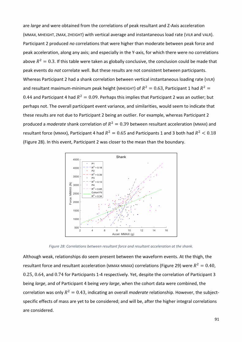
91
are large and were obtained from the correlations of peak resultant and Z-Axis acceleration
(MMAX, MHEIGHT, ZMAX, ZHEIGHT) with vertical average and instantaneous load rate (VILR and VALR).
Participant 2 produced no correlations that were higher than moderate between peak force and
peak acceleration, along any axis; and especially in the Y-axis, for which there were no correlations
above 𝑅2 = 0.3. If this table were taken as globally conclusive, the conclusion could be made that
peak events do not correlate well. But these results are not consistent between participants.
Whereas Participant 2 had a shank correlation between vertical instantaneous loading rate (VILR)
and resultant maximum-minimum peak height (MHEIGHT) of 𝑅2 = 0.63, Participant 1 had 𝑅2 =
0.44 and Participant 4 had 𝑅2 = 0.09. Perhaps this implies that Participant 2 was an outlier; but
perhaps not. The overall participant event variance, and similarities, would seem to indicate that
these results are not due to Participant 2 being an outlier. For example, whereas Participant 2
produced a moderate shank correlation of 𝑅2 = 0.39 between resultant acceleration (MMAX) and
resultant force (MMAX), Participant 4 had 𝑅2 = 0.65 and Participants 1 and 3 both had 𝑅2 < 0.18
(Figure 28). In this event, Participant 2 was closer to the mean than the boundary.
Figure 28: Correlations between resultant force and resultant acceleration at the shank.
Although weak, relationships do seem present between the waveform events. At the thigh, the
resultant force and resultant acceleration (MMAX-MMAX) correlations (Figure 29) were 𝑅2 = 0.40,
0.25, 0.64, and 0.74 for Participants 1-4 respectively. Yet, despite the correlation of Participant 3
being large, and of Participant 4 being very large, when the cohort data were combined, the
correlation was only 𝑅2 = 0.43, indicating an overall moderate relationship. However, the subject-
specific effects of mass are yet to be considered; and will be, after the higher integral correlations
are considered.

92
Figure 29: Correlations between resultant force and resultant acceleration at the thigh.
The previous results have shown substantial variability between the event correlation results for
individual participants. In fact, there were only four events that produced at least moderate
correlations (𝑅2 > 0.3) for all four participants. These somewhat higher correlations occurred at
the shank only and were between peak resultant and vertical force (MMAX, ZMIN) and peak axial
acceleration (XMAX, XHEIGHT). This may seem to indicate that the shank is the best location for
predicting peak force from acceleration. However, even these correlations had much variability:
for each of these four correlations, the minimums were between 𝑅2 = 0.33 to 0.35 and the
maximums between 𝑅2 = 0.72 to 0.79. In other words, no events had a correlation of 𝑅2 > 0.36
for every participant.
If these events were the only available data from which to predict impact dose, then these results
would suggest that they are inadequate for long term, inter-participant reliability. To be valid for
extended use, these predicted impact levels would need to be at a much high accuracy and in the
order of at least 80%.62 This would necessitate the obtaining of at least very large correlations in
every person.
Integration
As briefly mentioned above, the correlation between force and acceleration waveform integration
was almost perfect for Participant 2 at the shank. The correlation of the axial acceleration (XINTEG)
and vertical force (ZINTEG) integral was 𝑅2 = 0.93, which is almost perfect, as illustrated in Figure
62 Chapter 4.1.4, Result Validation.

93
30. This high correlation was consistent with the correlations from Participant 1 (𝑅2 = 0.90) and
Participant 4 (𝑅2 = 0.95) which were also almost perfect, but far greater than Participant 1 (𝑅2 =
0.50) which was only moderate.
Figure 30: Integration of the vertical force and axial acceleration waveforms.
In fact, every integration correlation across participants and locations was at least moderate, with
most correlations very large to almost perfect, as shown in Table 17. And on further consideration,
it is seen that the moderate correlation of Participant 1 was in fact a clear outlier.
Table 17: Correlations between the integration of force and acceleration.
Integration: Force-Acceleration
Thigh Shank Ankle
𝑹𝟐 Vertical-Axial* Resultant-Resultant** Vertical-Axial Resultant-Resultant Vertical-Axial Resultant-Resultant
P1 0.88 0.84 0.50 0.86 0.76 0.88
P2 0.92 0.91 0.93 0.91 0.97 0.94
P3 0.93 0.83 0.90 0.91 0.98 0.98
P4 0.92 0.79 0.95 0.92 0.91 0.90
Mean 0.91 0.85 0.82 0.90 0.91 0.92
Cohort 0.78 0.83 0.89 0.90 0.95 0.93
*Vertical Force (ZINTEG) - Axial Acceleration (XINTEG) **Force Magnitude (MINTEG) - Acceleration Magnitude (MINTEG)
Concluding on the participant means in Table 17, the optimal location for predicting the force
integral is the ankle, which produces a mean resultant and axial correlation almost equivalent to,
or greater than, the thigh and the shank (𝑝 < 0.05).63 Considering the entire cohort, the ankle is
also more effective than the thigh and shank (𝑝 < 0.03).
63 Almost equivalent was defined as a difference of not more than 𝑅2 = 0.01.

94
However, when comparing the vertical-axial participant correlations at the thigh (𝑅2 = 0.88 to
0.93) with the same cohort correlation (𝑅2 = 0.78), it is peculiar that the cohort regression value
was so low. To understand this, the effects of participant mass must be understood.
Further two-tailed paired-sample t-Tests were performed for calculating the statistical difference
between the original cohort and mass-scaled correlation differences.64 It was hypothesised for
each test that the means of the samples were the same (i.e. 𝐻0 = 0). The results show that
scaling by mass increases the cohort regression at every location for each integration correlation
between force (ZINTEG, MINTEG) and acceleration (XINTEG, MINTEG):
- The difference was statistically significant (𝑝 = 0.0027, 𝑀𝐷𝑅2= 0.02), so it was
statistically likely that mass had increased the regression coefficient.65
- The smallest increase was between resultant force and acceleration, where mass increased
the regression coefficient from 𝑅2 = 0.90 to 0.90 (the increase was 𝑅2 = 0.0031).
The effect of mass-scaling in the cohort regression is also shown above in the extension of Table
17 below, where the inclusion of mass increases every cohort correlation; and is further illustrated
in Figure 31.
Table 18: Extension of Table 17, showing the cohort mass-induced correlation differences.
Thigh Shank Ankle
𝑹𝟐 Vertical-Axial Resultant-Resultant Vertical-Axial Resultant-Resultant Vertical-Axial Resultant-Resultant
Cohort 0.78 0.83 0.89 0.90 0.95 0.93
Cohort:
mass-
scaled
0.83 0.85 0.90 0.90 0.96 0.95
64 All tests were calculated using the Microsoft Excel t-Test: Paired Two Sample for Means (two-tailed). 65 Average unscaled: 𝜇𝑅2 = 0.88; average mean-scaled: 𝜇𝑅2
𝑚𝑎𝑠𝑠= 0.90; mean difference 𝑀𝐷𝑅2 = 0.02.

95
Figure 31: Mass-scaled integral correlations. (A) Vertical force (ZINTEG) and axial acceleration (XINTEGMASS).
(B) Resultant force (MINTEG) and resultant acceleration (MINTEGMASS).
The prediction model for the integral of vertical force (ZINTEG) from mass-scaled axial acceleration
(XINTEGMASS) at the ankle can then be given as:
𝐹ZINTEG = 5367.3 + 0.13039 × 𝐴XINTEGMASS
This model returns a correlation accuracy of 𝑅2 = 0.96 and a root mean squared error of 𝑅𝑀𝑆𝐸 =
3.01 × 10⁴ 𝑁. 𝑠. Equivalently, this model can furthermore be expressed in terms of vertical
impulse:
𝐼𝑉⃗⃗ ⃗ = 5367.3 + 0.13039 × ∫𝐴𝑋⃗⃗⃗⃗ ⃗ 𝑑𝑡 × 𝑚𝑎𝑠𝑠
Cohort Mass-Scaled Event Correlations
In light of the favourable effect of mass-scaling that has been observed, event correlations were
also revisited with the inclusion of mass-scaling. Following an analysis of the cohort regression
results in Appendix A, the following event-to-event cohort-combined conclusions were made:
- Scaling by mass increased the cohort regression at every location between both peak
resultant and vertical force (MMAX, ZMIN) and every peak acceleration (MMAX, XMAX, YMAX,
ZMAX) (𝑝 < 0.0001).66
o Initial range: 0.10 < 𝑅2 < 0.54
66 Average unscaled: 𝜇 = 0.32; average mean-scaled: 𝜇𝑚𝑎𝑠𝑠 = 0.39; mean difference 𝑀𝐷𝑅2 = 0.07.
A B

96
o Mass-scaled range: 0.15 < 𝑅2 < 0.59
- Scaling by mass increased the cohort regression at every location between both vertical
loading rates (VALR, VILR) and every peak acceleration (MMAX, XMAX, YMAX, ZMAX) (𝑝 =
0.0105).67
o Initial range: 0.05 < 𝑅2 < 0.35
o Mass-scaled range: 0.07 < 𝑅2 < 0.35
The increase in correlations of peak resultant force (MMAX) and peak resultant acceleration (MMAX)
after scaling by mass (MMAXMASS) are shown in Figure 32, where it is observed that the cohort
correlations were highest at the thigh; then the shank; then the ankle.
Figure 32: Correlation differences after scaling by mass for resultant force (MMAX) and resultant acceleration (MMAX). (A) Direct correlations. (B) Mass-scaled correlations.
As shown above, the highest cohort correlation obtained at the thigh, which was between peak
resultant force (MMAX) and mass-scaled peak resultant acceleration (MMAXMASS), was 𝑅2 =
0.5769. Interestingly, between vertical force (ZMIN) and the same mass-scaled peak resultant
acceleration (MMAXMASS), the correlation was 𝑅2 = 0.5694, which is only a difference of -1.3%.68
The same resultant-resultant correlations from the shank and ankle were 𝑅2 = 0.45 and 0.27
respectively.
The highest correlation obtained at the ankle, which was between peak resultant force (MMAX)
and mass-scaled peak Y-axis acceleration (YMAXMASS), was 𝑅2 = 0.5364. Between vertical force
(ZMIN) and the same mass-scaled peak Y-axis acceleration (YMAXMASS), it was 𝑅2 = 0.5318
67 Average unscaled: 𝜇 = 0.19; average mean-scaled: 𝜇𝑚𝑎𝑠𝑠 = 0.20; mean difference 𝑀𝐷𝑅2 = 0.01. 68 Percent Decrease =
0.5694−0.5769
0.5769× 100 = −1.300%.
A B

97
(−0.86%).69 The same resultant-Y-axis correlations from the thigh and shank were 𝑅2 = 0.52 and
0.38 respectively.
The highest correlation obtained at the shank, which was between peak resultant force (MMAX)
and mass-scaled peak axial acceleration (XMAXMASS), was 𝑅2 = 0.5927. Between vertical force
(ZMIN) and the same mass-scaled peak axial acceleration (XMAXMASS) correlation of 𝑅2 = 0.5924
(−0.05%).70 The same resultant-axial correlations as obtained at the thigh and ankle were 𝑅2 =
0.29 and 0.25 respectively.
In each case, the vertical correlation was within 2% of the resultant correlation:
0.98 × 𝑅𝐹𝑀
2 < 𝑅𝐹𝑉
2 < 1.02 × 𝑅𝐹𝑀
2
Although these results were all only large (0.5 < 𝑅2 < 0.7), the proximity of these resultant and
vertical force correlations do indicate that the resultant magnitude of each waveform for both
acceleration and force in the recorded activities is primarily dependent on the magnitude of the
vertical force axis. In light of the previous investigation, where direct linear correlations have been
considered for individuals and for the entire cohort, the investigation will now turn to consider
whether these correlations can be improved with the application of a 20 Hz lowpass filter.
7.3.2. Filter-Induced Differences
Overview
This investigation must determine whether filtering the data using a lower cut-off frequency
prepares the acceleration data for predictive analysis more effectively than the previous 50 Hz
filter. Following the recommendations given by Simons and Bradshaw (2016), a 20 Hz filter will be
applied to the acceleration data, and if there are major differences between the results, may
inform this investigation of the location of the primary frequencies which contribute to the
efficacy of a predictive model.
To best understand the effect of a different filter, the entire correlation set will be compared.
However, it would be quite arduous to repeat the previous investigation and comment on the
change of every possible variable for both filters and with different models; for even at this stage,
69 Percent Decrease =
0.5318−0.5364
0.5364× 100 = −0.8576%.
70 Percent Decrease =0.5924−0.5927
0.5927× 100 = −0.0506%.

98
many correlations have not been considered.71 The decision was therefore made to perform a cell-
to-cell t-test for each correlation in the tables of Appendix A, with the aim of determining whether
the 20 Hz filtered correlation results were statistically different to the 50 Hz filter. If the 20 Hz filter
were found to produce statistically different results, the 20 Hz filtered data would be retained in
the following investigation; if the results were not statistically different, only the 50 Hz filtered
data would be retained.
Applying the 20 Hz Filter
Identical in all other regards to the previous filter of 50 Hz, a new 4th order Butterworth lowpass
filter with its poles at 20 Hz was designed and applied to the acceleration data. The effect that this
has to the waveform is shown in Figure 33, where the normal, 50 Hz filtered, and 20 Hz filtered
waveforms are compared for a trial of Participant 1. The change in the absolute maximum of this
waveform (i.e. the negative peak) due to the 50 Hz filter was +0.07%, and for the 20 Hz filter was
-18.3%.
Figure 33: Comparison of raw, 50 Hz filtered, and 20 Hz filtered acceleration data.
71 It would be quite impractical to comment on every correlation present in the tables of Appendix 2. So far, the investigation has attempted to summarise and explain the most informative and insightful correlations for the purpose of this investigation, but the summary which has been provided is by no means exhaustive of the potential meaning which could be wrought through a more extensive consideration of the entire correlation set. For what is possible, these considerations will be explained in more detail in the later discussion (Chapter 7.5), but this will be predominantly based on the information which has been explicitly mentioned in this investigation.

99
The same tables as in Appendix A were generated for the 20 Hz filtered data. A two-tailed paired t-
test was performed for each set within the generated correlations: the 50 Hz filtered correlations
from Participant 1 at the thigh were compared the 20 Hz filtered correlations from Participant 1 at
the thigh; etc. for each participant, location and cohort correlation. It was hypothesised for each
test that the mean difference was equal (i.e. 𝐻0 = 0). The results are shown below in Table 19.
Table 19: Comparison of correlation coefficients between 20 and 50 Hz filtered data. Green indicates a stronger
correlation.
Persons
P1Thigh P2Thigh P3Thigh P4Thigh
50 Hz Mean (𝑹𝟐) 0.2095 0.2191 0.2665 0.3497
20 Hz Mean (𝑹𝟐) 0.1542 0.1825 0.1881 0.2352
𝒑-𝒗𝒂𝒍𝒖𝒆 0.0002 0.0035 < 0.0001 < 0.0001
P1Shank P2Shank P3Shank P4Shank
50 Hz Mean (𝑹𝟐) 0.2001 0.2640 0.2104 0.3435
20 Hz Mean (𝑹𝟐) 0.1591 0.2082 0.1768 0.2454
𝒑-𝒗𝒂𝒍𝒖𝒆 0.0040 < 0.0001 0.0528 < 0.0001
P1Ankle P2Ankle P3Ankle P4Ankle
50 Hz Mean (𝑹𝟐) 0.1941 0.2191 0.1965 0.2266
20 Hz Mean (𝑹𝟐) 0.1390 0.1699 0.1648 0.1903
𝒑-𝒗𝒂𝒍𝒖𝒆 0.0001 0.0001 0.0362 0.0252
Cohort
Thigh Shank Ankle
50 Hz Mean (𝑹𝟐) 0.1985 0.2270 0.1768
20 Hz Mean (𝑹𝟐) 0.1463 0.1774 0.1506
𝒑-𝒗𝒂𝒍𝒖𝒆 < 0.0001 < 0.0001 0.0113
The null hypothesis was rejected in almost every test: the difference between the means of the 50
Hz- and 20 Hz filtered data is statistically significant. The one exception to this was for Participant
3 at the shank, where 𝑝 > 0.05 and the null hypothesis was not rejected. However, this seemed to
be an anomaly: aside from this one situation, the mean of the 50 Hz filtered data was greater than
the 20 Hz filtered data on every occasion. The statistical significance was in favour of the 50 Hz
filtered data, for on average, the 20 Hz filter actually reduced the correlations.
In the previous section, a consideration was made as to what correlations produced at least
moderate locations for all four participants. It was found that apart from the integral correlations,
this only occurred for the shank correlations between peak resultant and vertical force (MMAX,

100
ZMIN) and peak axial acceleration (XMAX, XHEIGHT). The same consideration was made to
understand the reduced 20 Hz filtered data correlations, and it was found that none of these
events achieved correlations of greater than 𝑅2 = 0.3 for all four participants.
However, there was one event correlation that produced at least moderate correlations for all four
participants in the 20 Hz filtered data. This was between peak resultant force (MMAX) and peak
resultant acceleration (MMAX) at the thigh, where the correlations were 𝑅2 = 0.42, 0.31, 0.47,
and 0.75 for each participant, respectively. These same resultant-resultant correlations in the 50
Hz filtered data were: 𝑅2 = 0.40, 0.25, 0.64, and 0.74 respectively. Several observations may be
made on this:
- Although the 20 Hz filter reduced most correlations, it did increase others, such that the 20
Hz filtered thigh data correlated higher for this event than the 50 Hz filtered data.
- The 20 Hz filter increased the location correlation consistency of single events at the thigh,
since values which were not consistently predictable at the shank between participants
were more consistently predictable at the thigh.
- Although the 20 Hz filter increased this correlation in comparison with the 50 Hz data and
shank correlations, the increase was not uniform across the correlations. The 20 Hz filtered
data for this event at this location was only higher for Participants 1, 2, and 4; for
Participant 3, the 50 Hz filtered data was still higher.
Similar to the 50 Hz filter, the 20 Hz filter obtained moderate to almost perfect integral
correlations of 𝑅2 = 0.47 to 0.98 (the 50 Hz filter had obtained 𝑅2 = 0.50 to 0.98). There were
no other events for which the 20 Hz filtered data obtained at least moderate correlations for more
than three participants. In light of all of these results, it was concluded that the 20 Hz filter does
not produce stronger correlations than the 50 Hz filter, and that the 50 Hz filter was overall more
effective.
Having determined that applying a 20 Hz filter does not, on average, increase the mean of the
event correlations, it was decided that all future analysis would continue using the 50 Hz filtered
dataset. The final validation method for determining the predictive power of these linear models
would be to determine the inter-participant predictive accuracy of the linear models with a leave-
one-out cross-validation study. However, since the previous results have shown that in general,
the events of this dataset do not have greater than large correlations, it was determined that a
cross-validation study would not add value to this investigation; for worse correlations would not

101
be practically useful, and higher correlations would be due to chance. Therefore, it was decided
that the only waveform characteristics that would be considered in the cross-validation study
were the 50 Hz filtered data integral correlations.
7.3.3. Leave-One-Out Cross-Validation for Linear Integration
Overview
The leave-out-out cross-validation will entail the development of a model based on the 50 Hz
filtered data of three participants, and then validating the model against the fourth participant.
This will provide an understanding into generalisable physiological waveform events, where if a
model were consistently accurate for a general population, the models can be assumed as
physiologically representative of a general population.72 Indeed, if there are not characteristic
relationships that are true for every participant, then it is expected that a cross-validation model
would enable the identification of this.
Method
This process will be completed four times per model, with a different participant left out each
time. This was chosen because if the conclusions of a single model were generalised over the
entire population, then they may misrepresent the actual resolving power of the model, since the
results generated may have only worked for that combination of training data. This would also
provide an understanding of how training sets can influence the results. This method necessarily
involves each model being trained without the data of the person on whom the model will be
validated, increasing the validity of the trained model. If the validation person’s data was included
in the training model, as it effectively was in the previous cohort correlations, then it is expected
that these results of an applied model would be high, since the model would have originally been
trained with the data of the validation participant, nullifying its predictive argument.
The method that will be used to perform this cross validation is illustrated in Figure 34. The
predicted values obtained from the model will be compared with the actual measured values.
72 Assuming that the four participants represent the general population.

102
Figure 34: Flow-structure for the cross-validation protocol.
This method will be used to determine the ability of the model to predict the activity force
integral, or impulse. Specifically, the variables that will be modelled and predicted are:
- Integration of resultant force with mass-scaled resultant acceleration (MINTEG-MINTEGMASS).
- Integration of vertical force with mass-scaled axial acceleration (ZINTEG-XINTEGMASS).
Because the correlations between uniaxial and resultant events are so similar,73 it is assumed that
these correlations will be similar again to the resultant-axial and vertical-resultant correlations;
and as such these will not also be tested.
Results
The data of Participants 1 to 3 were taken, from which a generalised linear model was developed.
The correlations are shown in Figure 35.
Figure 35: Developing a global model for the integration of force (impulse) from the data of Participants 1 to 3.
73 Chapter 7.3.1, Event-to-Event Correlations.

103
The global model that was developed from this regression is given directly and in terms of vertical
impulse:
𝐹ZINTEG = −54790.5388 + 7.3916 × 𝐴XINTEGMASS
𝐼𝑉⃗⃗ ⃗ = −54790.5388 + 7.3916 × ∫𝐴𝑋⃗⃗⃗⃗ ⃗ 𝑑𝑡 × 𝑚𝑎𝑠𝑠
This model was applied to the data of Participant 4, where Figure 36 shows the actual and
predicted values for the integration of vertical force, and the correlation accuracy of the actual
and predicted force.
Figure 36: Predicting the vertical force integral.
(A) Predicting the force integration of Participant 4 from the developed model.
(B) The correlation between predicted vs. actual force integration values for Participant 4.
As seen, the predicted model produced a correlation coefficient of 𝑅2 = 0.9147. When the
acceleration integral was originally correlated with the force integral at the ankle of Participant 4,
the correlation was also 𝑅2 = 0.9147. However, this should not be surprising, since all that has
occurred within this cross-validation is a shifting and scaling of the original acceleration values. As
such, a much better indicator of the effectiveness of this cross-validation method is to consider
the root mean squared error of the predicted data. These results for all participants and locations
are given in Table 20, with the cell that corresponds to the preceding analysis highlighted in blue in
the lower right corner.
To clarify, the errors given below are not direct equivalent comparisons because:
A B

104
- the original RMSE pertains to the correlation between the original FZINTEG and AXINTEGMASS,
whose magnitudes were in the order of 106 and 105, and therefore had an RMSE in the
order of 105.
- the predicted RMSE pertains to the correlation between the original FZINTEG and the
predicted FZINTEG, whose magnitudes were both in the order of 106, and therefore had an
RMSE in the order of 106.
As such, it is expected that the RMSE for the predicted force will be an order higher than the RMSE
of the original prediction; and as such, these results should be taken as relative indicators of
accuracy. Considering the results below, it can be seen that for every situation, the predicted
RMSE is between 4.4 to 13.6 times the size of the original error, as expected. It is therefore
reasonable to conclude that the cross-validation models have predicted force from acceleration to
a similar degree of accuracy as the original cohort correlations.
Table 20: Results of the linear Leave-One-Out investigation.
Comparison of Original vs. Predicted Force Integration
Left-Out Participant
Location
𝑹𝑴𝑺𝑬 (𝑵. 𝒔 × 𝟏𝟎𝟑) 3.s.f.
Resultant-Resultant Vertical-Axial
Original Predicted Original Predicted
Participant 1 Thigh 17.5 235 37.6 211
Shank 36.3 292 26.5 156
Ankle 25.9 191 29.8 141
Participant 2 Thigh 21.2 250 64.2 356
Shank 35.3 273 57.5 325
Ankle 31.3 233 70.8 356
Participant 3 Thigh 30.6 373 102 540
Shank 60.3 490 77.6 461
Ankle 26.8 194 47.1 209
Participant 4 Thigh 20.8 283 75.2 430
Shank 27.3 226 47.7 289
Ankle 33.4 247 56.5 267
Having considered the resolving power of linear models to relate the waveform characteristics of
acceleration and force, the investigation will now turn to consider non-linear prediction models:
namely, logarithmic and machine learning. This second phase will closely follow the methods as
presented in the present phase.
7.4. Phase 2: Non-Linear Modelling
The aim of Phase 2 is to determine whether the mass-scaled, 50 Hz filtered data is better
approximated by the previous linear, or by a logarithmic, correlation. The literature-identified

105
strategies for relating acceleration to force are logarithmic event-based modelling and machine
learning waveform modelling. These algorithms have been suggested for comparison according to
the literature models that produced three of the highest qualifications.74 Since there were no linear
event-to-event correlations in Phase 1 that for all participants produced correlations of 𝑅2 > 0.6,
Phase 2 will specifically target those events that produced moderate to large correlations in Phase
1, to see if these correlations can be improved by non-linear models.
7.4.1. Logarithmic Event Modelling
Overview
This section on logarithmic models will follow the method presented in a previous study by Charry
et al. (2013), who used the axial acceleration (XMIN, XMAX, XHEIGHT) of the shank to logarithmically
approximate peak vertical force (ZMIN).75 The initial model used by Charry et al. (2013) was:76
𝐹𝑉 = log2(𝐴𝑋 + 1)
However, they had then linearly generalised the formula according to participant mass:
𝐹𝑉(𝑚, 𝐴𝑋) = 𝑎(𝑚) + 𝑏(𝑚) × 𝑙𝑜𝑔2(𝐴𝑋 + 1)
In this formula, since log(𝐴𝑋) cannot be resolved with a real answer for 𝐴𝑋 ≤ 0, Charry et al.
(2013) included the shifting constant 𝑐 = 1 to account for any negative acceleration values.
However, although this was sufficient to correct their data, this did not account for any future
generalisation of this formula. Indeed, in the participant data of the present investigation, there
were values less than -1, which would have failed the model. To rectify this in the present
investigation, the entire dataset was linearly shifted according to the magnitude of the minimum
value in the dataset, normalising the trials such that the minimum value of each dataset was 1:
𝐹𝑉(𝑚, 𝐴𝑋) = 𝑎(𝑚) + 𝑏(𝑚) × 𝑙𝑜𝑔2(𝐴𝑋 + 𝑎𝑏𝑠(𝑚𝑖𝑛(𝐴𝑋)) + 1)
Results
Ordinarily, as was shown for the waveforms in the previous section, the direction of the vertical
force vectors is negative. However, it seemed more intuitive to present the logarithmic results in
terms of positive numbers, and as such, for this section on logarithms, the negative values for
74 See Chapter 4.2.3, Table 11. 75 Chapter 3.2.2, Non-Linear Models. 76 The notation used by Charry et al. (2013) has been changed here to reflect the common notation within this thesis.

106
vertical force (FZMIN) and axial acceleration (AXMIN) will be given as rectified displays. As this is only
a linear scaling of the output, there is no change in correlation. As a reference example, the linear
fit between vertical force (FZMIN) (which has been rectified) and axial acceleration (AXMAX) (which
did not need rectification) for Participant 1 is illustrated Figure 37.
Figure 37: Rectifying negative vertical force (ZMIN). (B) Original fit. (A) Rectified fit.
The effective equation that describes the rectified logarithmic fit in Figure 37 is:
𝐹𝑉 = 591.8 + 384.3 × log2(𝐴𝑋 + 𝑎𝑏𝑠(min(𝐴𝑋)) + 1)
This logarithmic fit of peak vertical force (ZMIN) can be also compared linearly with the actual peak
vertical force (ZMIN), as illustrated in Figure 38.
A
B
Rectified
Original

107
Figure 38: Logarithmic prediction of force (ZMIN) from acceleration (XMAX) against the actual value.
Comparing this relationship for each of the four participants, the logarithmic fit is found to have an
inconsistent effect, producing higher correlations for Participants 1 and 3; but lower for 2 and 4.
This data is summarised in Table 21.
Figure 39: Comparison of linear and logarithmic correlations between vertical force (ZMIN) and axial acceleration (XMAX).
(A) Participant 1. (B) Participant 2. (C) Participant 3. (D) Participant 4.
B
D
A
C

108
Table 21: Logarithmic models and respective correlations.
Individual Logarithmic Approximation Coefficients
𝒂 𝒃 𝑹𝟐 (Linear Fit) 𝑹𝟐 (Logarithmic Fit)
Participant 1 591.8 384.3 0.4956 0.4615
Participant 2 1196 301.0 0.3332 0.2972
Participant 3 733.1 461.4 0.4838 0.5624
Participant 4 -115.7 859.3 0.7865 0.5876
To demonstrate the application of this data to a general relationship, following the method of
Charry et al. (2013), let the coefficients 𝑎 and 𝑏 be assumed as linearly dependent on the mass of
each participant. Then, they can be plotted, and a linear relationship derived between them.
Applying the leave-one-out method, this has been calculated and illustrated for Participants 1, 2,
and 3 in Figure 40, in preparation for validating the model on Participant 4.77
Figure 40: Using linear approximations to obtain coefficients for the global logarithmic model. (A) a(m). (B) b(m).
These mass-derived coefficients may then be used to complete the logarithmic model:
𝐹𝑉(𝑚, 𝐴𝑋) = 𝑎(𝑚) + 𝑏(𝑚) × 𝑙𝑜𝑔2(𝐴𝑋 + 𝑎𝑏𝑠(𝑚𝑖𝑛(𝐴𝑋)) + 1)
𝑎(𝑚) = −1401.7495 + 32.0516 × 𝑚𝑎𝑠𝑠
𝑏(𝑚) = 295.6782 + 1.2375 × 𝑚𝑎𝑠𝑠
77 This method has clearly not obtained an accurate linear relationship between mass and the relative
coefficients, but it will be used to remain consistent with the method presented by Charry et al. (2013). In
light of these results, it is probably a reasonable assumption to say that these correlation coefficients are
not linearly related by mass. As it is, Charry et al. (2013) did not provide a correlation coefficient for this
part of their study, so the results of the coefficient linear fit cannot be directly compared.
A B

109
This model was applied to Participant 4 and the results are shown in Figure 39. Naturally, the new
logarithmic model will have the same correlation coefficient (𝑅2) and 𝑅𝑀𝑆𝐸 as the original log
model, since they are only a scaling and shifting of the original data values:
Figure 41: Comparison of the linear and logarithmic models for vertical-axial shank prediction.
Modelling for All Participants and Locations
The analysis was extended to the thigh and ankle, where in each case, one participant was left out
of development and used to test the model. The results of this extension are shown below in Table
22. 𝑅𝑀𝑆𝐸 cells are shaded green if they were lower (better) and red if higher (worse), where a
lower 𝑅𝑀𝑆𝐸 corresponds to a higher 𝑅2 value. The corresponding results of Participants 1-3 have
been included in Appendix B.
Table 22: Logarithmically modelling the vertical force and axial acceleration of Participant 4 at each location.
Results of Logarithmic Modelling
Participant Location Correlation 𝑹𝟐 𝑹𝑴𝑺𝑬 (𝑵)
Force Acceleration Linear Log Linear Log
4
Thigh
ZMIN XMAX 0.17 0.12 879.9 903.7
ZMIN XMIN 0.52 0.43 672.5 726.6
ZMIN XHEIGHT 0.36 0.31 774.7 804.9
Shank
ZMIN XMAX 0.79 0.59 445.5 619.3
ZMIN XMIN 0.47 0.44 699.0 722.8
ZMIN XHEIGHT 0.73 0.62 504.6 593.9
Ankle
ZMIN XMAX 0.17 0.22 884.6 857.2
ZMIN XMIN 0.02 0.04 957.2 947.4
ZMIN XHEIGHT 0.12 0.16 908.5 889.7
Although the correlation was higher in each ankle correlation, this was not indicative of the entire
dataset (c.f. Appendix B). To confirm this, a two-tailed paired t-test was performed on the

110
correlation coefficients of the linear set and the logarithmic set.78 It was found that the logarithmic
model correlation coefficients were overall not statistically different to the linear results (𝑝 =
0.39).
Cohort Prediction
However, where this has the greatest effect difference is when considering the combined cohort
correlation. In this case, although each participant will have been scaled and shifted linearly (and
so the intra-participant RMSE will not have changed), precisely because each data set has been
scaled differently, the cohort will have an overall different correlation.
In addition to performing this scaling of the function, the input to the function was changed from
being only peak axial acceleration (MMAX) to being mass-scaled peak axial acceleration
(MMAXMASS). To illustrate this, consider that if the above method is repeated for the entire cohort;
and Participants 1-3 are used to train the model; and where the data of every participant has been
individually scaled by their respective mass, then the model coefficients describing the
relationship between peak vertical force (ZMIN) and peak axial acceleration (XMAX), according to
𝐹𝑉(𝑚, 𝐴𝑋), are below. The graph generated by this is shown in Figure 42.
𝑎(𝑚) = 4677.9 − 76.7872 × 𝑚
𝑏(𝑚) = −1513.0 + 31.0445 × 𝑚
Figure 42: Cohort correlation of peak vertical force (MMAX) with peak axial acceleration (XMAX). (A) Comparison of correlations. (B) Cohort 𝐹𝑉(𝑚, 𝐴𝑋) predicted fit against the actual force.
78 The level of significance was set at 𝑝 = 0.05. Results: 𝜇𝐿𝑖𝑛𝑒𝑎𝑟 = 0.32, 𝜇𝐿𝑜𝑔 = 0.32, 𝑝 = 0.3943. The null
hypothesis was not rejected: the correlations between the linear and logarithmic models were not statistically different.
A B

111
Although this model for these events produced a correlation of 𝑅2 = 0.24 and an 𝑅𝑀𝑆𝐸 = 619,
and although there seems to be quite a large overestimation, what can be observed is that this fit
is actually closer to the linear fit than the original logarithmic fit was. The regression equation that
produced this correlation, shown in Figure 42 (B) was:
𝑦 = 858.43 + 0.18932 × 𝐹𝑉(𝑚, 𝐴𝑋)
This relationship may be visualised more clearly if the above prediction is scaled according to this
linear fit; the result of this is shown in Figure 43.
Figure 43: Adjusted predicted cohort fit.
Accounting for both 𝑦 and 𝐹𝑉(𝑚, 𝐴𝑋), the final equation form is written as:
The results of the remaining locations and events for Participant 4 are shown in Table 23. The
results of the model that was generated in Figure 42 and Figure 43 may be read in the top line of
this table. Because it was found in Phase 1 that mass increased linear model accuracy, only the
mass-scaled events were correlated here; except for the peak height (XHEIGHT), as this was not
𝑎(𝑚) 𝑏(𝑚)
𝑦 = 𝑎 + 𝑏 × ((𝑐 + 𝑑 × 𝑚) + (𝑒 + 𝑓 × 𝑚) × log2(𝐴𝑋 + 𝑎𝑏𝑠(min 𝐴𝑋) + 1))
𝐹𝑉(𝑚, 𝐴𝑋)

112
considered with respect to mass in the analysis.79 The cohort results of all four participants have
been included in Appendix B.
Table 23: Logarithmically modelling the vertical force and axial acceleration of the entire cohort at each location.
Results of Logarithmic Modelling
Participant Location Correlation 𝑹𝟐 𝑹𝑴𝑺𝑬 (𝑵)
Force Acceleration Linear Log Adjusted Log Linear Log Adjusted Log
4
Thigh
ZMIN XMAXMASS 0.29 0.16 0.24 601 650 619
ZMIN XMINMASS 0.42 0.36 0.23 541 567 623
ZMIN XHEIGHT 0.32 0.29 0.41 584 600 546
Shank
ZMIN XMAXMASS 0.59 0.39 0.44 449 552 528
ZMIN XMINMASS 0.30 0.27 0.21 589 602 627
ZMIN XHEIGHT 0.50 0.41 0.52 498 539 489
Ankle
ZMIN XMAXMASS 0.26 0.16 0.26 611 647 611
ZMIN XMINMASS 0.16 0.17 0.19 651 646 636
ZMIN XHEIGHT 0.19 0.20 0.31 637 635 589
The results lean in favour of the linear models: the linear model correlation coefficients were
statistically different to the original logarithmic results (𝑝 < 0.0001) and the adjusted logarithmic
results (𝑝 = 0.035), with the linear models higher in both cases (𝑀𝐷𝑅2 = 0.07 and 0.05).80 The
adjusted logarithmic model was not statistically different to the original logarithmic model (𝑝 =
0.27), but it was on average higher (𝑀𝐷𝑅2 = 0.02). Based on these results, there is not sufficient
evidence to affirm that the vertical force waveform is better approximated logarithmically than
linearly, and as such, the results of Charry et al. (2013) were not reproduced. The final part of
Phase 2 will now consider a machine learning model to see if this can possibly lift these lower
correlations.
7.4.2. Machine Learning Waveform Modelling
Overview
The purpose of using machine learning within this investigation was to consider the effectiveness
of an advanced non-linear timeseries algorithm to predict an output force from an input
acceleration series. These predictions were made in MATLAB, using the Deep Learning Toolbox.
This toolbox was chosen rather than manual design because the aim of this investigation was to
evaluate machine learning as a whole; not to determine whether a new kind of machine learning
79 But for the record, the mean of the mass-scaled logarithmic models (𝜇 = 0.27) was also higher than the un-scaled event data (𝜇 = 0.25). 80 Two-tailed paired t-test; level of significance: 𝑝 = 0.05. Results: 𝜇𝐿𝑖𝑛𝑒𝑎𝑟 = 0.34, 𝜇𝐿𝑜𝑔 = 0.27, 𝑀𝐷 =
0.07, 𝑝 = 0.016. Null hypothesis rejected: statistically different, linear models higher.

113
algorithm could be manually developed. Within this section, triaxial acceleration data will be used
to predict both vertical force (𝐹𝑍) and resultant force (𝐹𝑀).
Model Types
Since the peak events in the force and acceleration waveform do not occur simultaneously,81 then
if there is a relationship between them, it is probably time-dependent, based on the kinematics
preceding the peak. The Deep Learning Toolbox contains three types of predictive functions for
neural network timeseries modelling (MathWorks, 2020):
1) Non-linear auto-regressive with external exogenous input:
▪ Both the input 𝑥 and the output 𝑦 are fed as inputs into the transfer function.
y(t) = f(y(t – 1), . . . , y(t – d), x(t – 1), . . . , (t – d))
2) Non-linear autoregressive:
▪ Only the output 𝑦 is fed as an input into the transfer function.
𝑦(𝑡) = 𝑓(𝑦(𝑡 – 1), . . . , 𝑦(𝑡 – 𝑑))
3) Non-linear input-output:
▪ Only the input 𝑥 is fed as an input into the transfer function.
𝑦(𝑡) = 𝑓(𝑥(𝑡 – 1), . . . , 𝑥(𝑡 – 𝑑))
Model 1 would be useful for predicting the future values of stock or financial systems, and Model
2 for the control of various mechanical systems. However, since in a practical application of a
wearable device the actual force values will not be known and cannot be verified (without an
accompanying device), neither Models 1 nor 2 can be used for this investigation. Model 3, which
considers only the previous values of the input, is appropriate for the prediction of unknown force
values.
As previously, this model will be trained on three participants, and then tested against the fourth
participant. Note that whereas the previous sections had considered event-to-event correlations,
and as such only a single event per movement and waveform was considered, this section is
considering the entire waveform, and so will also display these similarities in terms of the full
81 See Chapter 3.2.4, Algorithm Variables.

114
waveform, rather than only in terms of point-to-point correlations. Prediction models for both
vertical and resultant force will be generated.
Data Preparation
All trial data at the shank was concatenated in the following way.
Let the concatenated axial acceleration data of Participant 1, for all trials, be written as:
𝐴𝑋𝑃1= [
𝐴𝑋𝑇𝑟𝑖𝑎𝑙 1
⋮𝐴𝑋𝑇𝑟𝑖𝑎𝑙 𝑛
]
Then for the triaxial data of each training participant, the model input can be written as:
Shank Input = [[
𝐴𝑋𝑃1
𝐴𝑋𝑃2
𝐴𝑋𝑃3
] [
𝐴𝑌𝑃1
𝐴𝑌𝑃2
𝐴𝑌𝑃3
] [
𝐴𝑍𝑃1
𝐴𝑍𝑃2
𝐴𝑍𝑃3
]]
The vertical force data of the test participant was similarly concatenated into an output array:
Shank Output = [
𝐹𝑍𝑃1
𝐹𝑍𝑃2
𝐹𝑍𝑃3
]
Data was divided randomly into a 70% training set (205,056 timesteps), a 15% validation set
(43,941 timesteps), and a 15% testing set (43,941 timesteps). The Levenberg-Marquardt training
algorithm was chosen over a Bayesian Regularisation or a Scaled Conjugate Gradient because it
typically requires less time than the others, though it uses more memory (MathWorks, 2020).
Non-Linear Input-Output Waveform Modelling
A non-linear input-output model was trained on the shank data. The network in Figure 44 was
designed for this purpose. Consistent with the default given within the toolbox, it was designed
with 10 hidden neurons and 2 delays.
Figure 44: Non-linear input-output network design.

115
The response of the network is shown in Figure 45, where it is seen that a substantial amount of
error was observed.
Figure 45: Non-linear network training. Vertical axes: force (N). Horizontal axes: time in samples, where 1 sample
equals 0.5ms.
Considering this waveform prediction sample-by-sample, the equivalent correlations for the
training, validation and testing datasets are shown in Figure 46.

116
Figure 46: Correlation of input and output samples following the waveform prediction.
The model produced a validation dataset 𝑅𝑀𝑆𝐸 = 217.6 𝑁, 𝑅2 = 0.41. When applied to
Participant 4, the model produced a validation dataset 𝑅𝑀𝑆𝐸 = 324.3 𝑁, 𝑅2 = 0.36. In each
case, the correlation and the RMSE of the test participant performed slightly poorer than the
training results: 𝑀𝐷𝑅2 = −0.08, 𝑀𝐷𝑅𝑀𝑆𝐸 = +28 𝑁. The method was applied also to the other
participant combinations, and the results are shown in Table 24.
Table 24: Correlation and RMSE results of non-linear input-output waveform modelling.
Non-Linear Input-Output Waveform Modelling
Training Participants Timesteps 𝑹𝟐 𝑹𝑴𝑺𝑬 (𝑵) Test Participant 𝑹𝟐 𝑹𝑴𝑺𝑬 (𝑵)
1,2,3 292,938 0.41 218 4 0.36 324
1,2,4 253,409 0.45 237 3 0.38 228
1,3,4 242,983 0.41 247 2 0.37 222
2,3,4 291,471 0.48 230 1 0.31 270
Average - 0.44 233 - 0.36 261
Furthermore, it may be noticed that the model that was tested on Participant 4 produced an RMSE
of 324 N. The original linear model for Participant 4 (non-prediction; direct correlation) for vertical
peak force (MMAX) and axial peak acceleration (XMAX) had an RMSE of 446 N. The machine learning

117
prediction model for the entire waveform has produced a correlation with less error than the
initial Participant 4 linear correlation of the single event.
Including Mass
Following this, the same investigation was performed where mass was included as an input into
the model, where mass is an array of the same size as each acceleration input, with every value in
the array equivalent to the particular participant mass:
𝑚𝑃1 = [𝑚⋮𝑚
]
Input = [[
𝐴𝑋𝑃1
𝐴𝑋𝑃2
𝐴𝑋𝑃3
] [
𝐴𝑌𝑃1
𝐴𝑌𝑃2
𝐴𝑌𝑃3
] [
𝐴𝑍𝑃1
𝐴𝑍𝑃2
𝐴𝑍𝑃3
] [
𝑚𝑃1
𝑚𝑃2
𝑚𝑃3
]]
The results of including as an input in the model is shown below in Table 25.
Table 25: Correlation and RMSE results of non-linear input-output waveform modelling, where mass has been included
as an input.
Non-Linear Input-Output Waveform Modelling
Training Participants Timesteps 𝑹𝟐 𝑹𝑴𝑺𝑬 (𝑵) Test Participant 𝑹𝟐 𝑹𝑴𝑺𝑬 (𝑵)
1,2,3 292,938 0.46 230 4 0.21 588
1,2,4 253,409 0.46 230 3 0.36 241
1,3,4 242,983 0.46 238 2 0.37 221
2,3,4 291,471 0.48 226 1 0.27 508
Average - 0.47 231 - 0.30 390
The inclusion of mass has not made a substantial difference to the accuracy of the model. The
average correlation coefficient of the training data has slightly increased (𝑀𝐷𝑅2 = +0.03), but the
average test data correlation coefficient reduced (𝑀𝐷𝑅2 = −0.06). In contrast to the clear
increase that mass produced in the linear models, this is surprising. However, since mass was
constant for each third of the training data, it likely did not provide value to the timeseries model,
for the model would have expected a series of fluctuating, interdependent points; not a static
value.
Resultant Force
The same method as above was repeated for determining resultant force, rather than for vertical
force. The results are shown in Table 26 and Table 27. The differences between the results of the

118
resultant force and vertical force data were not significant (𝑝𝑅2 = 0.40, 𝑝𝑅𝑀𝑆𝐸 = 0.60). Based on
these results, it can be concluded that the non-linear input-output model has used triaxial
acceleration data and predicted resultant force at least as well as it predicted vertical force, but
there was not a significant difference in the predictive power of the model between these
variables.
Table 26: Correlation and RMSE results of non-linear input-output waveform modelling.
Non-Linear Input-Output Waveform Modelling
Training Participants Timesteps 𝑹𝟐 𝑹𝑴𝑺𝑬 (𝑵) Test Participant 𝑹𝟐 𝑹𝑴𝑺𝑬 (𝑵)
1,2,3 292,938 0.45 218 4 0.35 333
1,2,4 253,409 0.42 248 3 0.41 230
1,3,4 242,983 0.42 247 2 0.40 222
2,3,4 291,471 0.49 232 1 0.34 272
Average - 0.45 236 - 0.38 264
Table 27: Correlation and RMSE results of non-linear input-output waveform modelling, where mass has been included
as an input.
Non-Linear Input-Output Waveform Modelling
Training Participants Timesteps 𝑹𝟐 𝑹𝑴𝑺𝑬 (𝑵) Test Participant 𝑹𝟐 𝑹𝑴𝑺𝑬 (𝑵)
1,2,3 292,938 0.48 208 4 0.31 420
1,2,4 253,409 0.45 244 3 0.29 314
1,3,4 242,983 0.49 237 2 0.38 227
2,3,4 291,471 0.49 233 1 0.21 470
Average - 0.48 231 - 0.30 358
Although the correlations of these machine learning models were nearly always only moderate,
they were still higher, on average, than the event-to-event correlation results of Phase 1: for
whereas only four correlations in Phase 1 had consistently measured above 𝑅2 = 0.3 in every
person, the machine learning algorithms have here predicted the entire waveform at an accuracy
above this.82
Having considered the resolving power of linear, logarithmic, and non-linear timeseries machine
learning models, a more comprehensive discussion will now ensue, to tie together both the
literature and the results of this investigation.
82 The correlations in Phase 1 that consistently produced 𝑅2 > 0.3 were for the shank between peak resultant and vertical force (MMAX, ZMIN), and peak axial acceleration (XMAX, XHEIGHT).

119
Chapter 8. Discussion
8.1. Investigation Discussion
The preceding investigation was undertaken to assess and validate the performance of several
acceleration-force models as presented within the literature. This section will summarise the
results of this investigation and use them to conclude on the investigation hypotheses. It will
provide a discussion on the challenges and limitations that were present in the investigation.
Finally, it will offer a selection of recommendations for future research in these areas and suggest a
strategy for this to proceed.
8.1.2. Synopsis
Having extracted 14 events from each acceleration waveform, and six events from each force
waveform, the acceleration and force data from 111 activities of four participants were linearly
correlated.
Phase 1
The only variables that had very large to almost perfect correlations for all participants and
locations were the integral correlations between resultant and vertical force (MINTEG, ZINTEG), and
resultant and axial acceleration (MINTEG, XINTEG). The exception to this was the result of Participant
1 at the shank, who obtained 𝑅2 = 0.50 between vertical force and axial acceleration; but this
was a clear outlier, with all other participant and location correlations above 𝑅2 = 0.76. These
integral correlations were the strongest at the ankle (𝑝 < 0.05), but in general were at least very
large at all locations. When each integral and waveform event was scaled according to participant
mass, the entire cohort correlations always increased (𝑝 = 0.0027). The highest mass-scaled
cohort integration correlation was between vertical force (ZINTEG) from mass-scaled axial
acceleration (XINTEGMASS) at the ankle. In terms of vertical impulse (𝐼𝑉 = 𝐹ZINTEG), this model was
expressed as:
𝐼𝑉⃗⃗ ⃗ = 5367.3 + 0.13039 × ∫𝐴𝑋⃗⃗⃗⃗ ⃗ 𝑑𝑡 × 𝑚𝑎𝑠𝑠
Although individual participants would at times show other strong event correlations, they were
generally not consistent between participants, with the strongest correlations of one participant
often being substantially higher than the others. The only four events that were at least moderate
(𝑅2 > 0.3) for all four participants occurred at the shank only and were between peak resultant

120
and vertical force (MMAX, ZMIN) and peak axial acceleration (XMAX, XHEIGHT). However, the
variability even between these was still significant (𝑅2 = 0.33 to 0.79), and there were no events
that had a correlation of 𝑅2 > 0.36 for every participant. These inter-participant differences often
reduced the entire cohort correlations, making them a better indicator of the weak strength of the
generalised physiological relationship. Scaling the cohort-combined events by mass increased the
cohort correlation at every location, between both peak resultant and vertical force (MMAX, ZMIN)
and every peak acceleration (MMAX, XMAX, YMAX, ZMAX) (𝑝 < 0.0001).
• The highest cohort event correlation coefficient of the investigation was obtained at the
shank, between peak resultant force (MMAX) and mass-scaled peak axial acceleration
(XMAXMASS) (𝑅2 = 0.59).
• The highest cohort event correlation at the thigh was between peak resultant force (MMAX)
and mass-scaled peak resultant acceleration (MMAXMASS) (𝑅2 = 0.58).
• The highest cohort event correlation at the ankle was between peak resultant force (MMAX)
and mass-scaled peak Y-Axis acceleration (YMAXMASS) (𝑅2 = 0.54).
The respective acceleration components were different between locations, which may indicate
that device location changes the variable that must necessarily be used as the primary indicator in
the model. If so, then these reflect the research of Takeda et al. (2009), who observed that
different locations contain different waveform components; and these components may be more
or less helpful depending on the location that they are observed. That these maximum events
were all quite similar may indicate that resultant force can similarly be predicted from any of these
three locations on the leg, but that the shank is slightly favourable for the prediction of these
events.
In each of the three maximum correlations, the relevant force event was the triaxial resultant
force. This may indicate that resultant force should be the target variable in future studies for the
correlation of acceleration with force. However, in each case, the vertical correlations between
the same variables were within 2% of the resultant correlations. This indicated that the resultant
magnitude of each waveform for both acceleration and force in the recorded activities was
primarily dependent on the magnitude of the vertical force axis.
The primary frequencies for force were under 100 Hz, and the primary frequencies for
acceleration were under 50 Hz; and these were the filters that had been initially designed for each
dataset, and for which the above results were obtained. Following the application of a 20 Hz filter

121
to the acceleration data, the event correlations did not on average increase; but rather decreased
the correlations (𝑝 > 0.05). However, there was one event that improved when compared to the
50 Hz filter: this was between peak resultant force (MMAX) and peak resultant acceleration (MMAX)
at the thigh (0.31 < 𝑅2 < 0.75); the same correlations in the 50 Hz data at the shank and ankle
had at least one participant with a correlation coefficient of 𝑅2 < 0.3. Similar to the
aforementioned integral correlation results, the 20 Hz filter also obtained moderate to almost
perfect integral correlations of 𝑅2 = 0.47 to 0.98. It was concluded in light of these that the 20 Hz
filter does not produce stronger correlations than the 50 Hz filter, and that the 50 Hz filter was
overall more effective.
To validate the high integral correlations of the 50 Hz experiment, a leave-one-out cross-validation
study was performed, wherein the data of three participants was used to develop a model that
was tested on the fourth participant. As the properties of the regression coefficient meant that
the applied linear models would not change the correlation of the acceleration values after
applying the new linear model, only the RMSE of the predicted force values was considered.
Although the results of the RMSE were one order of magnitude out, this was considered to not be
inaccurate since the comparison was considering actual force (106) against predicted force (106)
rather than actual force (106) against mass-scaled acceleration (105). As such, the linear integral
force-acceleration models were not considered to be substantially different when predicted by a
generalised model.
Phase 2
Logarithmic models were applied to the same 50 Hz filtered shank data of peak vertical force
(ZMIN) with axial acceleration (XMIN, XMAX, XHEIGHT) data to validate the study results of Charry et
al. (2013). The generated models were dependent on participant mass and were of the form:
𝐹𝑉(𝑚, 𝐴𝑋) = 𝑎(𝑚) + 𝑏(𝑚) × 𝑙𝑜𝑔2(𝐴𝑋 + 𝑎𝑏𝑠(𝑚𝑖𝑛(𝐴𝑋)) + 1)
The formulas of the coefficients 𝑎(𝑚) and 𝑏(𝑚) were generated by the results of three
participants, and the overall model was tested on the fourth. Overall, the logarithmic model
correlation coefficients were not statistically different to the linear results (𝑝 = 0.39). The method
was extended to the cohort correlations, where the same process was repeated, and in addition to
this, a second logarithmic equation was defined:
𝑦 = 𝑎 + 𝑏 × ((𝑐 + 𝑑 × 𝑚) + (𝑒 + 𝑓 × 𝑚) × log2(𝐴𝑋 + 𝑎𝑏𝑠(min 𝐴𝑋) + 1))

122
Neither of these cohort-applied logarithmic models increased the event correlations; however, the
mean of the adjusted logarithmic equation did produce slightly higher correlations than the
original logarithmic equation. The previous linear model correlation coefficients were statistically
different to both the original logarithmic results (𝑝 < 0.0001) and the adjusted logarithmic results
(𝑝 = 0.035), with the linear models higher in both cases (𝑀𝐷𝑅2 = 0.07 and 0.05). As such, the
results of Charry et al. (2013) were not reproduced, and it was concluded that vertical force is not
better approximated logarithmically than linearly.
Following the logarithmic investigation, a non-linear input-output timeseries machine learning
model was designed and applied to the data. Using triaxial acceleration as the input variable (𝑥)
and vertical force as the desired output (𝑦), the model designed was of the form:
𝑦(𝑡) = 𝑓(𝑥(𝑡 – 1), . . . , 𝑥(𝑡 – 𝑑))
Three participants were used to train each model, with the fourth used to test it. The average
training correlation coefficient was 𝑅2 = 0.44, and the average test coefficient was 𝑅2 = 0.36.
Considering that these results were predicting the entire waveform, rather than only events, this
was considered to be a better result than the linear approximations, which had produced only four
events that between participants had 𝑅2 > 0.3.
This process was then repeated using mass as a fourth input alongside the triaxial acceleration
data. Although the average training correlation coefficient slightly increased (𝑀𝐷𝑅2 = +0.03), the
average test data correlation coefficient reduced (𝑀𝐷𝑅2 = −0.06). It was concluded that
including participant mass did not substantially improve the model accuracy, but that since mass is
not technically a timeseries input, the limited change in accuracy was not unusual.
This machine learning process was finally repeated with resultant force as the desired output
rather than vertical force. The resultant and vertical force prediction correlations were not
statistically different (𝑝𝑅2 = 0.40, 𝑝𝑅𝑀𝑆𝐸 = 0.60).
8.1.2. Conclusions
Linear Modelling
Regarding waveform events, the correlation variance does not provide confidence for the future
use of these variables. Despite there being more moderate to very large correlations at the shank,
the correlations of FMMAX and FZMIN with AXHEIGHT and AXMAX were not consistently high, and as
such should not be used as accurate estimations. However, since there were more consistent

123
event correlations on the shank that correlated at least moderately, and since the ankle was found
to overall produce the best integral correlations, there seems to be evidence supporting the
notion that the lower limb is optimal for predicting force from acceleration.
Although the vertical and resultant force correlations were often almost equal, the acceleration
variables that produced these similar correlations were not similar between locations. Rather,
different acceleration axes were found to be more or less correlated. The literature had
recommended that triaxial accelerometers be used (Elvin et al., 2007), and the evidence seems to
suggest that triaxial devices are indeed necessary to determine strong correlations. However, Elvin
et al. (2007) was the only study that actually used uniaxial accelerometers, so in light of these
results their recommendation towards triaxial devices is justified.
That the vertical average and instantaneous loading rates did not correlate well was surprising in
light of the large correlations produced by Davis et al. (2018). However, they had used a sample
size of 𝑛 = 169, where each participant ran for eight steps (in total, 1,325 events); whereas the
present investigation had only a sample size of 𝑛 = 4 with a combined 135 events from different
activities. In light of this, there was highly likely not substantial evidence to reject the conclusions
of Davis et al. (2018) based on the results of the present investigation.
Despite the waveform events generally not correlating consistently, the acceleration integral did
consistently and strongly correlate with the force integral. The prediction of integrals may
therefore bode well for the future of impact dose prediction; and especially when linearly scaled
according to participant mass. That this was high also seems to align with the literature, for as
Hunter et al. (2005) explains, “when horizontal, braking, propulsive, and vertical impulses [i.e.
force integration] are expressed relative to body mass, they reflect the change in velocity [i.e.
acceleration] of the center of mass… during the respective periods and in the respective directions.”
In this case, the ankle is the optimum position to place this to detect the highest acceleration
forces, since this is going to be the closest to the foot accelerations which were highest as
measured within this study. These positive results at the ankle are promising in the case of an
eventual device implementation, especially considering the preference of athletes to use this
lower location.83 However, expanded research will be required to determine the repeatability of
these results with a larger sample size. These differences between location hold further relevance
in understanding future implementation, especially regarding the position on each segment. When
83 Chapter 1.1.2, Considering a Device.

124
the device was placed on the ankle (near the distal tibia), versus on the shank (the medial tibia),
the results were different, and when applied in real life, the location will most certainly vary in
these small ways between participants.
When compared to the results that were originally obtained by Corbo (2018), it is found that the
results are substantially and surprisingly different. The highest correlation obtained by Corbo
(2018) was R2 = 0.64, which was also between the integration of vertical force and axial
acceleration at the ankle. With the correlations of the present investigation being approximately
𝑅2 = 0.3 higher for this same variable, it is likely that the analysis method used between the
original evaluation and the present re-evaluation was different. In the study by Corbo (2018), force
threshold, noise filtering and an activity start time had not been included; and in the present
investigation, the events selected for analysis had been re-evaluated for validity, with several
events used in the previous analysis discarded, and some retained that may not have been used
previously; so there were several differences in analysis that may have contributed to this. As the
exact method of analysis that was used by Corbo (2018) was not known, understanding the cause
of the correlation differences may not be possible.
Filtering
In the present investigation, although the thigh generally did not produce stronger correlations
than the shank or ankle, this is not to say that the thigh is sub-optimal in all circumstances. After
the 20 Hz filter had been applied, there was one particular thigh event correlation that increased
for every participant beyond what the 50 Hz filtered shank and ankle correlation for that event
had produced. There may therefore be particular waveform characteristics of the thigh that are
better for predicting different events, especially if the particular frequencies of that event are
isolated; and vice versa for the shank and ankle. This may confirm the notion that a single location
is not necessarily the best for predicting every feature, but that different locations are more
helpful for predicting different waveform features. This would be consistent with the earlier
discussion which showed that different waveform features are present at different locations
(Takeda et al., 2009). Generally speaking, across all locations, the events that included frequencies
between 0 to 50 Hz predicted force more accurately than when only the 0 to 20 Hz waveform
content had been considered.
In the literature, it had been recommended that lowpass filters with poles between 20 to 50 Hz be
further considered when predicting force from acceleration (Simons and Bradshaw, 2016). In the

125
present investigation, both of these filters were used: 50 Hz was experimentally chosen, and 20 Hz
was chosen following this recommendation from Simons and Bradshaw (2016). However, no
significant positive difference in the analysis was found, meaning that either the results of Simons
and Bradshaw (2016) were not generalisable to the kind of investigation that was here performed;
of that its application in the present investigation was errant because of systematic problems in
the dataset.
In light of these results, the conclusion from Simons and Bradshaw (2016) that resultant
acceleration filtering is more important that peak force-acceleration agreements does not seem to
hold true, for it was found that the filter did not make a significant differences, which was more in
line with the results of Rantalainen et al. (2018), who had also found no major differences. From
the present investigation, it would sooner be concluded that identifying force-acceleration
agreement is more important than understanding which filter to use. However, it is expected that
these two procedures are not mutually exclusive of each other: understanding the frequency
components of the acceleration data may be totally necessary for determine which events are the
events that cause an agreement; and therefore, although the application of these filters is
important, they may be secondary to understanding which events are the desired events for
correlation. These results also seem to justify the recommendation by the literature that higher
frequencies be further considered in future studies (Lafortune et al., 1995, Wundersitz et al.,
2013).
To be sure, filters must be chosen carefully, based on the targeted frequency content of each
activity and the elimination of noise. The optimal filter will inform not only which physiological
events correlate the strongest, but also of the frequency content of those events. However, this all
assumes that impact dose is optimally predicted by event-to-event correlations, and as such is not
necessarily exhaustive of the use or validity of the noise-eliminated raw data for the purpose of
predicting impact dose.
Logarithmic Modelling
The logarithmic modelling in the present investigation was based closely upon the work of Charry
et al. (2013), but did not replicate their results for the conditions that were specified. Whereas
Charry et al. (2013) had produced very large to almost perfect correlations, this investigation at
most only produced large correlations; and this was fairly uncommon. Charry et al. (2013) had
three participants, so the differences were not likely due to sample size. It is expected that the

126
differences primarily arose due to the activity variations that were involved in the present
investigation, for Charry et al. (2013) only had their participants run.
Charry et al. (2013) had only recorded their acceleration data at 100 Hz, but without their data, it
is not possible to determine whether this caused significant differences in the recording ability of
their device when compared to the 148.1 Hz of the present investigation. These relatively lower
sampling rates may have missed the sharper accelerations during breaking or pushing off in the
change of direction tasks. Without a second reference point for validating the acceleration in
addition to the accelerometers, it is not possible to determine this. Although it is not expected
that the recorded acceleration in the present investigation peaked during these sharp activities,
the higher dynamic range of ± 24 g that Charry et al. (2013) used may have provided an advantage.
Regarding the actual logarithmic model, the present investigation linearly shifted the acceleration
data according to the magnitude of the minimum axial acceleration data of each event set;
whereas Charry et al. (2013) had simply shifted their dataset by +1. This will have slightly changed
the correlation coefficient due to the properties of logarithmically scaling, but it is not expected
that this was the primary cause of why the correlation difference between studies was in excess of
𝑅2 = 0.3.84 Rather, it is expected that the primary cause of the reduced correlations was due to
the activity type and the shape of the model. Between linear and logarithmic modelling, for a
sample set characterised by that within this investigation, linear modelling is superior.
Machine Learning Modelling
The non-linear input-output timeseries neural network did not approximate force higher than
moderately, and as such cannot be concluded as a reliable method for predicting force from
acceleration. However, the fact that it produced an overall correlation coefficient of 𝑅2 > 0.3,
indicates that on average it has performed more favourably than the linear correlations, since the
linear models only had several events that correlated above this for every participant. However,
the events that did correlate linearly, for the entire cohort, correlated more strongly than the
machine learning model.
The results of the machine learning algorithms in this section cannot be directly compared with
the machine learning studies in the literature review because the neural network training models
were different between these. This indicates the different predictive abilities of different models
84 Maximum logarithmic correlations: Charry et al. (2013): 𝑅2 = 0.95; this investigation: 𝑅2 = 0.59.

127
for different purposes, as was explained in the investigation. However, it might actually be
possible that the method used by Guo et al. (2017) would not be applicable for a wearable device,
because it seems that their training algorithm incorporated known force values, using a model
similar to what was proposed as for a stock market. The results of an individual in any
commercialised device would never be confirmed though an accurate validation of true force. It is
uncertain whether the method used by Guo et al. (2017) is implementable for this kind of
approximation. However, in the long term, a model which, based on the known force values of a
large training set during manufacturing may become generalisable to an unknown future user, if
subject specific characteristic can be understood and implemented within this algorithm such that
it in effect becomes an input-output, rather than a model relying on known force data.
The weak resolving power of the neural network may further indicate that the acceleration data
lacked key information that contributes to the prediction of force. Perhaps this could be resolved
in a future machine learning model by including information from a gyroscope or magnetometer.
Any future model will also need to consider that whilst a real-time output is ideal, a complicated
machine learning algorithm may be limited in its application due to its power requirements and
the time that may be necessary to evaluate the model. As Pieper et al. (2020) has said, “the tuning
required from such methodology introduces distinct challenges which may limit the ease of
translation.”85
Mass
In every model, except the machine learning timeseries model, the inclusion of mass increased the
cohort and predictive model correlations, demonstrating the importance of the subject-specific
relationship. If these relationships and methods are to be generalised, it may be helpful to
establish the kind of participants for whom they may apply. It could be proposed that the results
of Participant 3 may provide insight into the relevance of these results to the general netball
population, for this participant was female and was closest to the mean weight of netballers; and
Participant 3 was representative of the mean mass of the trial participants:
i. The mean mass of elite female netballers has been reported as 73.42 ± 6.95 kg
(Simpson et al., 2019). The mass of Participant 3 was 73.97 kg (+0.75% elite mean
mass).
85 This was stated in conclusion to their study on random forest networks.

128
ii. The mean mass of all four participants was 72.99 kg. Participant 3 was +1.35% of this
mean participant mass. Participant 2 (male, 72.65 kg) was also closer to mean
participant mass (-0.46% mean).
However, it must be considered that the training set was not entirely representative of elite
netballers, since it included two non-elite males. As such, although Participant 3 may be the
closest in mass, since the model was not developed from a representative population, these
results may not be generalisable. But then again, because the results did include non-
representative participants, they may actually inform a more generalised model, since there is no
certainty as to the end user; only generalised estimates can be used for this. Alas, these
conclusions are still limited, for the sample size and inclusion is not likely sufficient to describe the
general population of elite netballers.
Challenges in Analysis
There were many system variables that could not be isolated or controlled within the
investigation, and the influence of which therefore could not be knowingly accounted for. For
example, it is expected that a major contributor to the inter-participant correlation differences
were different landing techniques. If a generalisable model for all subjects was to be developed, it
would need to incorporate the differences that are present in groups, including for amateur
athletes with inconsistent techniques and for those with physical limitations due to impairment.
Perhaps there is a generalised population dataset on which a model could be trained, such that
these predictive algorithms are more representative of a future user. As mentioned, the variety of
movements that were recorded in this investigation made it difficult to directly answer or validate
the movements of each other study. But this is not to say that a variety of movements cannot
produce strong correlations, because Meyer et al. (2015) had obtained very large correlations
using a similar variety of movements with 13 participants with devices placed on the hip. Due to
the number of different variables present between each study and movement, it is difficult to
isolate the precise cause of these differences.
Although the variance between activities may have been a contributing factor to the wide range of
correlations, understanding that the similarities between different movements in the future may
make multi-activity studies easier to compare and apply to other sports. Callaghan et al. (2018)
had recommended that an understanding of segment kinematics be provided regarding pace
bowling performance. Although pace bowling performance was clearly not considered in the

129
present investigation, the two-foot land and the cut may have been similar in that both
movements involve a sharp movement deceleration (the landing of both feet and the change of
direction) which are similar to the sharp planting of the single foot during a delivery. So, although
bowling was not specifically considered, such movements may contribute understanding to similar
activities and therefore be generalisable between different sports.
A summary of factors that have been raised within this report, by which the relationship is
affected, and between which a relationship may be modelled, are shown in Figure 47. These
factors are not necessarily mutually exclusive of one another, and it is likely that there are more
factors that were not considered in this investigation that have not been included in this summary.
Figure 47: Factors that contribute to model predictions, ascertained from the literature.
8.1.3. Limitations
The limitations of the investigation will now be considered. These have been outlined in five main
areas: study design, physiology, hardware, analysis, and research.
Study Design
The investigation had a limited sample size of 𝑛 = 4, wherein the participants had masses of
between 63.2 to 82.0 kg (range: 18.9 kg, +29.8%). It is expected that a more normalised
distribution of sample points provided by a larger cohort size would have provided more insight
into the physiological accuracy of the presented models. Although the inclusion of mass was found
to positively increase the cohort correlations, precisely how, why, and in what capacity this occurs
was not studied, for the investigation primarily focused on the efficacy of different predictive
models. However, this may be simply due to the kinematics of movement being consistent with
Newton’s Second Law of Motion, 𝐹 = 𝑚 × 𝑎.

130
As the available patient data did not include information on their physical health before or after
the trial, the consideration of kinematics in relation to injuries could not be determined. As such,
these results cannot be generalised to a population with physiological impairments. Although
noise-attenuating filters were applied to the acceleration data, the study was not able to
determine and account for the effects of soft tissue attenuation between participants and
locations that may have been present within the selected frequency range.
The study was confined to a laboratory environment, and so cannot be generalised to external
environments or for environments with wind resistance or uneven terrain. The physical
characteristics of the footwear of each participant was not available, so differences between
participants due to this were considered as unknown systematic errors and were not accounted
for.
Physiology
The participants were not elite athletes and did not necessarily have the same level of fitness, and
as such the results cannot be generalised directly to elite athletes. Furthermore, since the study
did not consider how leg dominance affects technique, but only generalised these results by
position, and the results may have been skewed due to the inclusion of unequal leg support during
landing. The two contralateral devices therefore provided insight into combined, position-based
predictions, but not into the kinematics of a single location. This decision had been originally made
to increase the sample size by pooling the event data from both legs, but rather than increasing
the distribution due to the greater amount of data, this may have actually limited the results by
masking any potential side-specific correlations. If leg dominance had further been incorporated
into this, and if the dominant leg was the leg that carried the most impact during these
movements (as it may have done during the change-of-direction movements), then the leg-
specific dominant-side data may have produced more consistent and comparable relationships.
In addition to not considering single placements, the investigation also did not consider multiple
locations. As only the ankle, shank, and thigh were individually investigated, the literature-based
results pertaining to the other locations could not be validated, and as such although the lower leg
was here identified as optimal, this is not globally conclusive regarding all potential locations. This
is particularly so for the logarithmic and machine learning estimations, which were only calculated
on the shank.

131
Within the qualified articles, several had recorded cyclic activities; but the present investigation
only considered single movements. Therefore, these cyclic-movement studies cannot be validated
according to the generated results. However, these studies lack the generalisability to a wide
range of movements, and their results must be applied accordingly. Although the movements that
were compared included a range of speed variations and models, the exact contribution of the
different events remains unknown. Although the waveforms of each event were visually sighted
during the analysis, the shape of each waveform was not formally analysed, so the exact means
behind the conjecture that different events have largely contributed to the variance in results is
yet to be proven for this dataset. It had been suggested in the literature that the average of
several events from multiple strides be used to predict calculations, rather than only correlating
the events of individual strides (Raper et al., 2018). As this was not considered in the study, the
benefits of using this method could not be evaluated; and considering the variability of the data,
this method may have been quite helpful. Alas, only a selection of variables and analysis methods
could be chosen for consideration.
Hardware
There were also several technological limitations present. As the study did not have access to
gyroscopic output, joint and contact angles could not be considered; meaning that angular
acceleration could not be considered. Global vertical acceleration was not correlated with vertical
force, which may have produced different correlations according to the linear 𝐹 = 𝑚 × 𝑎 model.
Although it did not seem that acceleration had peaked, since the literature said that accelerations
can be up to 12 g, the 9 g accelerometers used may not have correctly captured the kinematics of
every activity.
However, if the high magnitude accelerations were also generated at high frequencies, then the
devices may have missed them anyway, because the sampling rate of the accelerometer was quite
low (148.1 Hz). The available data was therefore jagged, and the analysis had to be completed
based on the approximated waveform via a filter. It is impossible to know whether the events that
were analysed were true representations of the physiological magnitudes. To get a more accurate
representation and prediction, a higher sampling rate may be necessary.
This study did not consider the presence of internal device bias. This was predominantly due to
only having access to the trial data, rather than being able to test the measurement ability of the
devices and calibrate them prior to the data analysis. Several of the original devices that were

132
used by Corbo (2018) had been replaced due to failure, and for the ones that remained, the bias
present would not have been accurate to the state of the device during the original recording. It
had to be assumed that the device specifications given in the original device documentation and in
the previous study were indeed representative of the true original device performance.
Analysis
The analysis was limited in that it did not assess every potential acceleration or force event and
did not exhaust the list of potential models by which these events may be related. Fourier and
event-based machine learning were two models that were presented in the literate but were not
validated. The conclusion must not be made that waveforms do not correlate, but only that the
strategies that were used here to model these events were not effective for producing strong
correlations.
It was assumed that the filters that were applied were acceptable for both datasets, with the
original filters being applied only to remove non-physiological noise. However, the design of the
filter was based on the results of a single trial and may not have been indicative of the primary
frequencies of every waveform. Although 50 Hz had been recommended in the literature as a filter
to consider, there may have been high power frequencies that were filtered out, significantly and
unfavourably reducing the respective waveforms; but confirming this would require further
investigation.
After the 20 Hz filter was later applied on the data, and poor results obtained, 20 Hz filtered data
was put aside, assumed to not produce stronger correlations than the 50 Hz filtered dataset. Since
the effectiveness of this filter for non-linear modelling was not validated, the conclusion that the
20 Hz filter resulted in weaker correlations than the 50 Hz filter is limited to prediction via the
linear models demonstrated.
Several conclusions were made based on the statistical significance generated by t-tests. Although
these do not seem inappropriate considering the context, it is acknowledged that other kinds of
statistical analysis could have been used to demonstrate the strength of correlations in additional
ways. It is also assumed that even though several of the t-tests used in this investigation did not
have more than eight samples per group, their conclusions need not be rejected simply because
they are small (Bland and Altman, 2009).
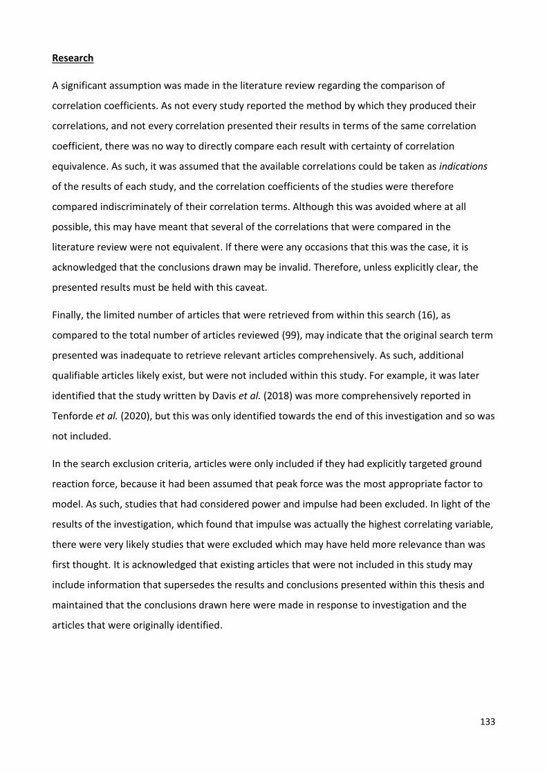
133
Research
A significant assumption was made in the literature review regarding the comparison of
correlation coefficients. As not every study reported the method by which they produced their
correlations, and not every correlation presented their results in terms of the same correlation
coefficient, there was no way to directly compare each result with certainty of correlation
equivalence. As such, it was assumed that the available correlations could be taken as indications
of the results of each study, and the correlation coefficients of the studies were therefore
compared indiscriminately of their correlation terms. Although this was avoided where at all
possible, this may have meant that several of the correlations that were compared in the
literature review were not equivalent. If there were any occasions that this was the case, it is
acknowledged that the conclusions drawn may be invalid. Therefore, unless explicitly clear, the
presented results must be held with this caveat.
Finally, the limited number of articles that were retrieved from within this search (16), as
compared to the total number of articles reviewed (99), may indicate that the original search term
presented was inadequate to retrieve relevant articles comprehensively. As such, additional
qualifiable articles likely exist, but were not included within this study. For example, it was later
identified that the study written by Davis et al. (2018) was more comprehensively reported in
Tenforde et al. (2020), but this was only identified towards the end of this investigation and so was
not included.
In the search exclusion criteria, articles were only included if they had explicitly targeted ground
reaction force, because it had been assumed that peak force was the most appropriate factor to
model. As such, studies that had considered power and impulse had been excluded. In light of the
results of the investigation, which found that impulse was actually the highest correlating variable,
there were very likely studies that were excluded which may have held more relevance than was
first thought. It is acknowledged that existing articles that were not included in this study may
include information that supersedes the results and conclusions presented within this thesis and
maintained that the conclusions drawn here were made in response to investigation and the
articles that were originally identified.

134
8.1.4. Hypothesis Conclusion
In the Investigation Outline (Chapter 7.1), six hypotheses were made regarding the development
of an acceleration-force relationship. Based on the results of the investigation, each of these will
now be concisely concluded on as either supported or rejected, followed by a brief explanation.
1. There is a very large relationship (𝐑𝟐 = 𝟎. 𝟕 to 𝟎. 𝟗) between force and acceleration at
the lower limb, with the shank being optimal for developing this model.
Supported
With the exception of a single outlier (𝑅2 = 0.5), the participant correlations between the
integrals of force (resultant and vertical) and acceleration (resultant and axial) at every location
were very large to almost perfect (𝑅2 = 0.76 to 0.98). However, there were no waveform events
that correlated consistently above 𝑅2 = 0.36 for all participants, and in this regard the hypothesis
is rejected.
2. The shank is the most effective position for modelling this relationship.
Rejected
The strongest correlations were measured between the integrals of force and acceleration at the
ankle (𝑝 < 0.05). However, participant and cohort correlation were also at least very large
between the integral of resultant force and acceleration at the shank (𝑅2 = 0.86), so although the
shank was not the most effective, it was yet highly effective.
3. Generalised models are the most effective when they incorporate subject-specific
characteristics.
Supported
On average, the inclusion of mass increased the cohort regression value between the integral of
force and acceleration by 𝑅2 = 0.02 (𝑝 = 0.0027). Scaling by mass also increased the cohort
regression values of every peak force and acceleration event (𝑝 = 0.0001).
4. The correlations after filtering the data with a 20 Hz filter will be higher than when the
data is only filtered for noise.
Rejected

135
For every participant and cohort correlation set, except for Participant 3 at the shank, the
correlations between the 50 Hz and the 20 Hz filtered data models were statistically significant
(𝑝 < 0.05), and in every instance the mean correlation of the 50 Hz models was greater.
5. Logarithmic modelling predicts force more accurately than linear modelling.
Rejected
The linear model correlation coefficients were statistically different to all logarithmic models
results (𝑝 < 0.05), with the linear models higher in both cases (𝑀𝐷𝑅2 > 0.05).
6. Machine learning modelling predicts force more accurately than logarithmic and linear
modelling.
Supported
Although the correlations of the machine learning models were nearly always only moderate, with
an entire waveform predictive ability of up to 𝑅2 = 0.41, they were on average higher than the
linear and logarithmic event-to-event correlation results.
8.2. Future Research
Finally, having considered the conclusions of the investigation, this section outlines areas of
research that are yet to be explored. It is followed by a very brief recommendation for the
continuance of this project.
8.2.1. Future Research Areas
The following list of research areas have been collated to summarise the areas that have been put
forward in this thesis as necessary objectives towards further research in this field. These
recommendations include research that may inform the prediction of impact risk from impulse,
and also regard how waveform event correlations may be further considered and improved upon.
Injuries
• Determine whether the established relationship between the force and acceleration
waveform integrals can be used as an indicator for impact dose and used to quantify injury
risk.
• Determine whether other waveform event correlations can be improved for this end and
determine what locations are optimal for recording these values.

136
• Determine precisely how this information relates to injuries and identify an objective count
of impact dose.
• Determine how fatigue affects technique and prediction model accuracy.
• Determine how post-injury recovery will affect the performance of a prediction model, and
in what capacity a predictive model may be used to assess and aid rehabilitation programs
such as following ACL reconstruction.
• In Figure 48, an arbitrary risk measurement assessment has been generated to
demonstrate the application of this future research. In this, the peak forces from each
activity of each individual have been given. This arbitrary indication has been designed with
the assumption that level of risk may depend on the ability of a person to adapt their
technique to deal with landing force, and therefore that the risk level at the same forces
may differ between people.
Figure 48: Conceptualising the long-term goal of this research - a risk scale generated for resultant peak force.
Activities and Technique
• Determine how specific activity types contribute towards model kinetics.
• Consider whether a model that identifies movement and uses an algorithm to predict the
force based on the identified movement can make an effective prediction model design.

137
• Determine how differences in landing technique change prediction accuracy and how the
models should adapt to a change in technique over time.
• Determine the primary factors that contribute to inter-participant correlation variability.
• Determine how participant athletic ability affects model accuracy across age, gender, skill,
and impairment.
• Determine whether leg dominance is an indicator of model performance; and whether the
kinematics of one leg can predict the kinematics of the other leg; and whether leg-specific
performance is important for model accuracy.
• Determine whether the effects of footwear and terrain (e.g. timber vs. concrete) must be
factored into the model, or whether the effects of these are negligent.
• Determine whether the kind of knee and ankle stabilisation braces as frequently worn by
netball players86 diminishes propulsive power and will inhibit the accuracy of a predicted
model.
Data Analysis
• Determine activity frequency components such that an appropriate sampling frequency
can be selected.
• Determine exactly what portion of the frequency spectrum pertain to the events that
correlate and design filters accordingly.
• Determine whether acceleration in the global vertical axis or in the transverse plane (as
relative to the axial axis) are beneficial for load prediction.
• Determine whether different and applicable machine learning models are more effective at
modelling force with acceleration than the non-linear input-output timeseries neural
network that was used in this investigation.
o Consider single event prediction rather waveform prediction.
o Perhaps consider sinusoidal or polynomial approximation models.
• Consider revisiting linear and logarithmic correlations following a large, uniform, single-
activity cohort study.
86 Chapter 1.1.2, Considering a Device.

138
Study Design
• Determine whether it is necessary to first validate a prediction model for a single kind of
movement, rather than a range of different movements. This may eliminate the variability
of results as obtained in the preceding investigation.
o Perhaps consider undertaking a cyclic activity study.
• Eventually, design a study that collects data from a comprehensive list of activities, such
that the force prediction of any activity that may be monitored with the device can be
validated.
• Determine inter-session location repeatability and effect (i.e. whether minimal placement
changes dramatically negatively affect model prediction accuracy).
• Determined how the presence of movement artefact and soft tissue attenuation can be
detected, perhaps through a calibration routine with a motion capture system. Use this
information to determine an optimal method for securing the device to remove such noise.
• Determine an effective method of device attachment such that movement artefact is
minimised.
o Perhaps undertake a study in which several people are given different kinds of
devices, collecting information on overall device preference, comfortability, and
intrusive features.
8.2.1. Recommended Priority
In light of all that has been considered, the following steps are a recommended as a way forward:
1. Determine whether and in what way impulse can be used as a measure of impact dose,
and how this can contribute to injury prevention and a measure of participant risk.
2. Identify or design a wearable accelerometer that has minimum movement artefact when
attached.
3. Conduct a trial with a large sample size in an attempt to reproduce the high integration
correlation results and prove the relevance of the prediction for overuse injury risk.

139
Chapter 9. Thesis Conclusion
9.1. Conclusion
Having reviewed the literature and undertaken an investigation into the characteristics of the
force-acceleration relationship, the preceding research will now be concluded on.
9.1.1. Conclusion
The aim of this investigation was to determine whether there is a relationship between force and
acceleration at the lower limb that can be accurately modelled using data from wearable
accelerometers; and whether this relationship can be generalised across subjects, movements,
and external conditions such that it is useful for injury management and prevention.
This research has demonstrated that there is a relationship between ground reaction force and
acceleration at the lower limb. But, as seen in both the literature and in the investigation, this
relationship is highly dependent on activity, technique, model, and data preparation, and it may
be observed to produce inconsistent results. The results of the validation investigation were not
consistent with the literature-based correlations, but this was likely due to variance in study
design, cohort size, and activities undertaken in the trial.
The strongest relationship identified was between the integration of force, which is impulse, and
acceleration. This was consistently very large to almost perfect across participants, and the highest
linear correlation was obtained at the ankle. Although the shank and thigh also produced, on
average, at least very large impulse correlations, the ankle lateral malleolus was generally higher
and was deemed optimal. The strongest correlation at the ankle was between vertical force and
axial acceleration. The variability of results may indicate that although a relationship is present, it
may not be immediately generalisable between subjects, movements, and external conditions.
The small cohort used in the present investigation did not produce consistently high event-based
correlations. Although the linear and logarithmic models were at times able to predict accurately
between events, the results between participants were not consistent. The best indicator of
event-based relationships was the global cohort averages. These indicated that the force
magnitude increases with acceleration magnitude, but that there are many challenges that must
be yet overcome before the accuracy of these inter-person results will be consistent. As the
machine learning model that was applied did not predict the force waveform above a moderate
accuracy, it was deemed more accurate than the linear and logarithmic event modelling. With the
qualification that there were no correlations that consistently measured above moderate in all

140
models (except for integration at the ankle), the medial shank was determined to be the most
accurate location from which to predict force waveform events.
The study has demonstrated both from the literature and from the investigation that an accurate
relationship between force and acceleration can be modelled using wearable accelerometers.
However, the accuracy variance between literature studies and this investigation demonstrated
that there are factors deeper than surface acceleration that contribute to an accurate model of
force. The generalised relationships produced a similar degree of accuracy as the subject-specific
models, but the variability between studies indicates that further research is necessary to confirm
the global validity of these models.
The investigation was unable to contribute to an understanding of injury prediction and objective
impact dose, but based on the literature, there does seem to be clinical relevance for the
prediction of force from acceleration. Future research must now consider precisely how these
objective kinematic quantities can be used to define an objective and accurate assessment of risk
level between individuals. Future studies should consider larger cohorts and determine whether
the results of this investigation can be reproduced. If an objective measure of injury risk can be
established, and be objectively quantified in terms of these results, then the strong relationships
that have been observed may become a broadly used level of preventative and rehabilitative
study.
The sooner that these safe dosage levels can be quantified, the sooner that this technology can be
applied in aiding chronic pain and reducing the risk of overuse injury for elite and non-elite
athletes, and in both rehabilitation and physiological monitoring.

141
References…
ABDELHADY, M., VAN DEN BOGERT, A. J. & SIMON, D. 2019. A High-Fidelity Wearable System for
Measuring Lower-Limb Kinetics and Kinematics. IEEE Sensors Journal, 19, 12482-12493.
ALAQTASH, M., YU, H., BROWER, R., ABDELGAWAD, A. & SARKODIE-GYAN, T. 2011. Application of
wearable sensors for human gait analysis using fuzzy computational algorithm. Engineering
Applications of Artificial Intelligence, 24, 1018-1025.
ALAQTASH, M., YU, H., BROWER, R., ABDELGAWAD, A., SPIER, E. & SARKODIE-GYAN, T. 2010.
Application of Wearable Miniature Non-invasive Sensory System in Human Locomotion
Using Soft Computing Algorithm, Berlin, Heidelberg, Berlin, Heidelberg: Springer Berlin
Heidelberg.
ANTONSSON, E. K. & MANN, R. W. 1985. The frequency content of gait. Journal of biomechanics,
18, 39-47.
ARAMI, A., AMINIAN, K., FORCHELET, D. & RENAUD, P. 2014. Implantable and wearable
measurement system for smart knee prosthesis.
AUSTRALIAN FOOTBALL LEAGUE 2019. Laws of Australian Football, Melbourne, Victoria.
BAILEY, A. M., MCMURRY, T. L., SALZAR, R. S. & CRANDALL, J. R. 2018. An Injury Risk Function for
the Leg, Foot, and Ankle Exposed to Axial Impact Loading Using Force and Impulse. Journal
of Biomechanical Engineering, 141.
BAILEY, J. A., GASTIN, P. B., MACKEY, L. & DWYER, D. B. 2017. The Player Load Associated With
Typical Activities in Elite Netball. Int J Sports Physiol Perform, 12, 1218-1223.
BERNARDS, J. R., SATO, K., HAFF, G. G. & BAZYLER, C. D. 2017. Current Research and Statistical
Practices in Sport Science and a Need for Change. Sports (Basel), 5, 87.
BEST, G. 2017. EPIDEMIOLOGY AND INCIDENCE OF INJURY IN ELITE NETBALL PLAYERS - AN INJURY
AUDIT OF THE 2016 NETBALL SUPERLEAGUE SEASON. British Journal of Sports Medicine,
51, 297.
BISSELL, L. & LORENTZOS, P. 2018. The prevalence of overuse injuries in Australian non-elite
netballers. Open Access Journal of Sports Medicine, 9, 233+.
BLAND, J. M. & ALTMAN, D. G. 2009. Analysis of continuous data from small samples. BMJ, 338,
a3166.
BOBBERT, M. F., YEADON, M. R. & NIGG, B. M. 1992. Mechanical analysis of the landing phase in
heel-toe running. Journal of Biomechanics, 25, 223-234.

142
BROWNE, M. G. & FRANZ, J. R. 2019. Ankle power biofeedback attenuates the distal-to-proximal
redistribution in older adults. Gait & Posture, 71, 44-49.
BRUCE, O. L., FIRMINGER, C. R., WANNOP, J. W., STEFANYSHYN, D. J. & EDWARDS, W. B. 2019.
Effects of basketball court construction and shoe stiffness on countermovement jump
landings. Footwear Science, 11, 171-179.
BRUKNER, P. D. & BENNELL, K. L. 2020. Chapter 3 - Stress Fractures: Their Causes and Principles of
Treatment.
CALLAGHAN, S. J., LOCKIE, R. G., ANDREWS, W. A., CHIPCHASE, R. F. & NIMPHIUS, S. 2018. The
relationship between inertial measurement unit-derived ‘force signatures’ and ground
reaction forces during cricket pace bowling. Sports Biomechanics, 1-15.
CHARRY, E., WENZHENG, H., UMER, M., RONCHI, A. & TAYLOR, S. 2013. Study on estimation of
peak Ground Reaction Forces using tibial accelerations in running. IEEE Eighth International
Conference on Intelligent Sensors, Sensor Networks and Information Processing.
CLARK, K. P., RYAN, L. J. & WEYAND, P. G. 2014. Foot speed, foot-strike and footwear: linking gait
mechanics and running ground reaction forces.(Report). Journal of Experimental Biology,
217, 2037.
CLARK, K. P., RYAN, L. J. & WEYAND, P. G. 2017. A general relationship links gait mechanics and
running ground reaction forces. The Journal of experimental biology, 220, 247-258.
COLBY, J. M., DAWSON, J. B., HEASMAN, J. J., ROGALSKI, J. B. & GABBETT, J. T. 2014.
Accelerometer and GPS-Derived Running Loads and Injury Risk in Elite Australian
Footballers. Journal of Strength and Conditioning Research, 28, 2244-2252.
CORBO, E. 2018. The Design and Development of a Wearable Device to Assess Lower-Limb Impact
Dose during Competitive Netball Play. Flinders University.
COVENTRY, E., O’CONNOR, K. M., HART, B. A., EARL, J. E. & EBERSOLE, K. T. 2006. The effect of
lower extremity fatigue on shock attenuation during single-leg landing. Clinical
Biomechanics, 21, 1090-1097.
CROWELL, H. P. & DAVIS, I. S. 2011. Gait retraining to reduce lower extremity loading in runners.
Clinical Biomechanics, 26, 78-83.
DAN, M. J., LUN, K. K., DAN, L., EFIRD, J., PELLETIER, M., BROE, D. & WALSH, W. R. 2019. Wearable
inertial sensors and pressure MAT detect risk factors associated with ACL graft failure that
are not possible with traditional return to sport assessments. BMJ Open Sport & Exercise
Medicine, 5.

143
DAVIS, I., HAYANO, T. & TENFORDE, A. 2018. The Relationship Between Vertical Loadrates and
Tibial Acceleration Across Footstrike Patterns. Foot & Ankle Orthopaedics, 3.
DEVITA, A. P. & SKELLY, A. W. 1992. Effect of landing stiffness on joint kinetics and energetics in
the lower extremity. Medicine & Science in Sports & Exercise, 24, 108-115.
EHRMANN, E. F., DUNCAN, S. C., SINDHUSAKE, N. D., FRANZSEN, A. W. & GREENE, A. D. 2016. GPS
and Injury Prevention in Professional Soccer. Journal of Strength and Conditioning
Research, 30, 360-367.
ELVIN, N., ELVIN, A. & ARNOCZKY, S. 2007. Correlation between Ground Reaction Force and Tibial
Acceleration in Vertical Jumping. Journal of applied biomechanics, 23, 180-9.
FÉDÉRATION INTERNATIONALE DE VOLLEYBALL 2016. Official Volleyball Rules 2017-2020.
FUTRELL, E. E., GROSS, K. D., REISMAN, D., MULLINEAUX, D. R. & DAVIS, I. S. 2020. Transition to
forefoot strike reduces load rates more effectively than altered cadence. Journal of Sport
and Health Science, 9, 248-257.
GABBETT, J. T. & ULLAH, J. S. 2012. Relationship Between Running Loads and Soft-Tissue Injury in
Elite Team Sport Athletes. Journal of Strength and Conditioning Research, 26, 953-960.
GOKELER, A., WELLING, W., ZAFFAGNINI, S., SEIL, R. & PADUA, D. 2017. Development of a test
battery to enhance safe return to sports after anterior cruciate ligament reconstruction.
Knee Surgery, Sports Traumatology, Arthroscopy, 25, 192-199.
GUO, Y., STORM, F., ZHAO, Y., BILLINGS, S. A., PAVIC, A., MAZZÀ, C. & GUO, L.-Z. 2017. A New
Proxy Measurement Algorithm with Application to the Estimation of Vertical Ground
Reaction Forces Using Wearable Sensors. Sensors (Basel, Switzerland), 17.
HAVENS, K. L., COHEN, S. C., PRATT, K. A. & SIGWARD, S. M. 2018. Accelerations from wearable
accelerometers reflect knee loading during running after anterior cruciate ligament
reconstruction. Clinical Biomechanics, 58, 57-61.
HENNIG, E. & LAFORTUNE, M. Tibial bone and skin accelerations during running. Cotton CE,
Lamontagne M, Robertson DGE, Stothart JPProceedings of the Fifth Biennial Conference of
the Canadian Society for Biomechanics. Ottawa: Spodym Publishers, 1988. 74-5.
HENNIG, E. & LAFORTUNE, M. A. 1991. RELATIONSHIPS BETWEEN GROUND REACTION FORCE AND
TIBIAL BONE ACCELERATION PARAMETERS. International Journal Of Sport Biomechanics, 7,
303-309.
HOPKINS, W. 2006. A New View of Statistics: A Scale of Magnitudes for Effect Statistics [Online].
Available: http://www.sportsci.org/resource/stats/index.html [Accessed 29 August 2020].

144
HOPKINS, W. G., MARSHALL, S. W., BATTERHAM, A. M. & HANIN, J. 2009. Progressive Statistics for
Studies in Sports Medicine and Exercise Science. Medicine & Science in Sports & Exercise,
41.
HOPPER, D. & ELLIOTT, B. 1993. Lower limb and back injury patterns of elite netball players. Sports
Med, 16, 148-62.
HOPPER, D., ELLIOTT, B. & LALOR, J. 1995. A descriptive epidemiology of netball injuries during
competition: a five year study. British Journal of Sports Medicine, 29, 223.
HUME, P. A. & STEELE, J. R. 2000. A preliminary investigation of injury prevention strategies in
netball: Are players heeding the advice? Journal of Science and Medicine in Sport, 3, 406-
413.
HUNTER, J. P., MARSHALL, R. N. & MCNAIR, P. J. 2005. Relationships between ground reaction
force impulse and kinematics of sprint-running acceleration. Journal of applied
biomechanics, 21, 31-43.
INTERNATIONAL BASKETBALL FEDERATION 2020. 2020 Official Basketball Rules: Basketball Rules &
Basketball Equipment, Mies, Switzerland.
INTERNATIONAL NETBALL FEDERATION 2020. Rules of Netball, 21-23.
JACOBS, D. A. & FERRIS, D. P. 2015. Estimation of ground reaction forces and ankle moment with
multiple, low-cost sensors. Journal of NeuroEngineering and Rehabilitation, 12.
JIANG, X., GHOLAMI, M., KHOSHNAM, M., ENG, J. J. & MENON, C. 2019. Estimation of Ankle Joint
Power during Walking Using Two Inertial Sensors. Sensors (Basel, Switzerland), 19.
KIERNAN, D., HAWKINS, D. A., MANOUKIAN, M. A. C., MCKALLIP, M., OELSNER, L., CASKEY, C. F. &
COOLBAUGH, C. L. 2018. Accelerometer-based prediction of running injury in National
Collegiate Athletic Association track athletes. Journal of Biomechanics, 73, 201-209.
LAFORTUNE, M. A. 1991. Three-dimensional acceleration of the tibia during walking and running.
Journal of Biomechanics, 24, 877,881-879,886.
LAFORTUNE, M. A., LAKE, M. J. & HENNIG, E. 1995. Transfer function between tibial acceleration
and ground reaction force. Journal of Biomechanics, 28, 113-117.
LAFORTUNE, M. A., LAKE, M. J. & HENNIG, E. M. 1996. Differential shock transmission response of
the human body to impact severity and lower limb posture. Journal of biomechanics, 29,
1531-1537.
LEE, Y.-S., HO, C.-S., SHIH, Y., CHANG, S.-Y., RÓBERT, F. J. & SHIANG, T.-Y. 2015. Assessment of
walking, running, and jumping movement features by using the inertial measurement unit.
Gait & Posture, 41, 877-881.

145
LEWIS, L. M., NAUNHEIM, R., STANDEVEN, J., LAURYSSEN, C., RICHTER, C. & JEFFORDS, B. 2001. Do
Football Helmets Reduce Acceleration of Impact in Blunt Head Injuries? Academic
Emergency Medicine, 8, 604-609.
LIIKAVAINIO, T., BRAGGE, T., HAKKARAINEN, M., JURVELIN, J. S., KARJALAINEN, P. A. & AROKOSKI,
J. P. 2007. Reproducibility of Loading Measurements With Skin-Mounted Accelerometers
During Walking. Archives of Physical Medicine and Rehabilitation, 88, 907-915.
MACADAM, D. P., SIMPERINGHAM, B. K. & CRONIN, B. J. 2017. Acute Kinematic and Kinetic
Adaptations to Wearable Resistance During Sprint Acceleration. Journal of Strength and
Conditioning Research, 31, 1297-1304.
MACWILLIAMS, B. A., COWLEY, M. & NICHOLSON, D. E. 2003. Foot kinematics and kinetics during
adolescent gait. Gait & Posture, 17, 214-224.
MAHDAVIAN, M., ARZANPOUR, S. & PARK, E. J. Motion Generation of a Wearable Hip Exoskeleton
Robot Using Machine Learning-Based Estimation of Ground Reaction Forces and Moments.
2019 IEEE/ASME International Conference on Advanced Intelligent Mechatronics (AIM), 8-
12 July 2019 2019. 796-801.
MARIN, F., LEPETIT, K., FRADET, L., HANSEN, C. & BEN MANSOUR, K. 2020. Using accelerations of
single inertial measurement units to determine the intensity level of light-moderate-
vigorous physical activities: Technical and mathematical considerations. J Biomech, 107,
109834.
MATHWORKS. 2020. Shallow Neural Network Time-Series Prediction and Modeling [Online].
Available: https://www.mathworks.com/help/deeplearning/gs/neural-network-time-
series-prediction-and-modeling.html [Accessed 9 October 2020].
MCMANUS, A., STEVENSON, M. R. & FINCH, C. F. 2006. Incidence and risk factors for injury in non-
elite netball. Journal of Science and Medicine in Sport, 9, 119-124.
MERO, A. 1988. Force-Time Characteristics and Running Velocity of Male Sprinters during the
Acceleration Phase of Sprinting. Research Quarterly for Exercise and Sport, 59, 94-98.
MEYER, U., ERNST, D., SCHOTT, S., RIERA, C., HATTENDORF, J., ROMKES, J., GRANACHER, U.,
GÖPFERT, B. & KRIEMLER, S. 2015. Validation of two accelerometers to determine
mechanical loading of physical activities in children. Journal of Sports Sciences, 33, 1702-
1709.
MUNDT, M., KOEPPE, A., DAVID, S., WITTER, T., BAMER, F., POTTHAST, W. & MARKERT, B. 2020.
Estimation of Gait Mechanics Based on Simulated and Measured IMU Data Using an
Artificial Neural Network. Frontiers in bioengineering and biotechnology, 8, 41-41.

146
NETBALL AUSTRALIA. 2016. Footwork and Movement skills [Online]. Available:
https://www.youtube.com/watch?v=rtnDm52t_eM [Accessed 13 October 2020].
NETBALL AUSTRALIA. 2019. Netball continues to lead for women and girls [Online]. Available:
https://netball.com.au/news/netball-continues-lead-women-and-girls [Accessed 8 October
2020].
NOSHADI, H., DABIRI, F., AHMADIAN, S., AMINI, N. & SARRAFZADEH, M. 2013. HERMES: Mobile
system for instability analysis and balance assessment. ACM Transactions on Embedded
Computing Systems (TECS), 12, 1-24.
PENGHAI, W., HAIYANG, Q. & LIDONG, L. 2014. A Wireless Wearable Human Jump Analysis
System. International journal on smart sensing and intelligent systems, 7.
PIEPER, N. L., LEWEK, M. D. & FRANZ, J. R. 2020. Can shank acceleration provide a clinically feasible
surrogate for individual limb propulsion during walking? Journal of Biomechanics, 98.
PRADKO, F., LEE, R. A. AND GREENE, J. D., BYARS, E. F., CONTINI, R. & ROBERTS, V. L. 1967. Human
vibration-response theory, in: Biomechanics monograph, American Society of Mechanical
Engineers.
PUYAU, M. R., ADOLPH, A. L., VOHRA, F. A. & BUTTE, N. F. 2002. Validation and calibration of
physical activity monitors in children. Obes Res, 10, 150-7.
RANTALAINEN, T., GASTIN, P. B., SPANGLER, R. & WUNDERSITZ, D. 2018. Concurrent validity and
reliability of torso-worn inertial measurement unit for jump power and height estimation.
Journal of Sports Sciences, 36, 1937-1942.
RAPER, D. P., WITCHALLS, J., PHILIPS, E. J., KNIGHT, E., DREW, M. K. & WADDINGTON, G. 2018. Use
of a tibial accelerometer to measure ground reaction force in running: A reliability and
validity comparison with force plates. Journal of Science and Medicine in Sport, 21, 84-88.
REENALDA, J., MAARTENS, E., HOMAN, L. & BUURKE, J. H. 2016. Continuous three dimensional
analysis of running mechanics during a marathon by means of inertial magnetic
measurement units to objectify changes in running mechanics. Journal of Biomechanics,
49, 3362-3367.
ROUHANI, H., FAVRE, J., CREVOISIER, X. & AMINIAN, K. 2014. A wearable system for multi-segment
foot kinetics measurement. Journal of Biomechanics, 47, 1704-1711.
SAZONOV, E. S., FULK, G., HILL, J., SCHUTZ, Y. & BROWNING, R. 2011. Monitoring of Posture
Allocations and Activities by a Shoe-Based Wearable Sensor. IEEE Transactions on
Biomedical Engineering, 58, 983-990.
147
SCHNEUER, F., BELL, J., ADAMS, S., BROWN, J., FINCH, C. & NASSAR, N. 2018. The burden of
hospitalized sports-related injuries in children: an Australian population-based study,
2005–2013. Injury Epidemiology, 5, 1-10.
SCOTT, S. H. & WINTER, D. A. 1993. Biomechanical model of the human foot: Kinematics and
kinetics during the stance phase of walking. Journal of Biomechanics, 26, 1091-1104.
SHAHABPOOR, E. & PAVIC, A. 2017. Measurement of Walking Ground Reactions in Real-Life
Environments: A Systematic Review of Techniques and Technologies. Sensors (Basel,
Switzerland), 17.
SIMONS, C. & BRADSHAW, E. J. 2016. Do accelerometers mounted on the back provide a good
estimate of impact loads in jumping and landing tasks? Sports Biomechanics, 15, 76-88.
SIMPSON, M. J., JENKINS, D. G., LEVERITT, M. D. & KELLY, V. G. 2019. Physical profiles of elite, sub-
elite, regional and age-group netballers. Journal of Sports Sciences, 37, 1212-1219.
STEVENSON, M. R., HAMER, P., FINCH, C. F., ELLIOT, B. & KRESNOW, M. 2000. Sport, age, and sex
specific incidence of sports injuries in Western Australia. British journal of sports medicine,
34, 188-194.
TAKEDA, R., TADANO, S., TODOH, M., MORIKAWA, M., NAKAYASU, M. & YOSHINARI, S. 2009. Gait
analysis using gravitational acceleration measured by wearable sensors. Journal of
Biomechanics, 42, 223-233.
TALUKDER, A. 2020. The design and development of a wearable device to assess lower-limb impact
dose during competitive netball play. Masters by Coursework, Thesis (Masters).
TAN, T., STROUT, Z. A. & SHULL, P. B. 2020. Accurate impact loading rate estimation during
running via a subject-independent convolutional neural network model and optimal IMU
placement. IEEE Journal of Biomedical and Health Informatics, 1-1.
TAO, L., INOUE, Y., SHIBATA, K. & RENCHENG, Z. 2007. Measurement of human lower limb
orientations and ground reaction forces using wearable sensor systems.
TENFORDE, A. S., HAYANO, T., JAMISON, S. T., OUTERLEYS, J. & DAVIS, I. S. 2020. Tibial
Acceleration Measured from Wearable Sensors Is Associated with Loading Rates in Injured
Runners. PM&R, 12, 679-684.
TONG, K. & GRANAT, M. H. 1999. A practical gait analysis system using gyroscopes. Medical
Engineering and Physics, 21, 87-94.
TRAN, J., NETTO, K., AISBETT, B. & GASTIN, P. 2012. Validation of accelerometer data for
measuring impacts during jumping and landing tasks.

148
UDOFA, A. B., RYAN, L. J. & WEYAND, P. G. 2016. Impact forces during running: Loaded questions,
sensible outcomes.
WILLY, R., BUCHENIC, L., ROGACKI, K., ACKERMAN, J., SCHMIDT, A. & WILLSON, J. 2016. In‐field
gait retraining and mobile monitoring to address running biomechanics associated with
tibial stress fracture. Scandinavian journal of medicine & science in sports, 26, 197-205.
WINTER, M. E. 2005. JUMPING: POWER OR IMPULSE? Medicine & Science in Sports & Exercise, 37,
523-523.
WORLD RUGBY. 2019. World Rugby Handbook: Regulation 12. PROVISIONS RELATING TO PLAYERS’
DRESS [Online]. Available: https://www.world.rugby/handbook/regulations/reg-12
[Accessed 4 September 2020].
WOUDA, F. J., GIUBERTI, M., BELLUSCI, G., MAARTENS, E., REENALDA, J., VAN BEIJNUM, B. F. &
VELTINK, P. H. 2018. Estimation of Vertical Ground Reaction Forces and Sagittal Knee
Kinematics During Running Using Three Inertial Sensors. Front Physiol, 9, 218.
WUNDERSITZ, D. W., GASTIN, P. B., RICHTER, C., ROBERTSON, S. J. & NETTO, K. J. 2015. Validity of
a trunk-mounted accelerometer to assess peak accelerations during walking, jogging and
running. European journal of sport science, 15, 382-390.
WUNDERSITZ, D. W. T., NETTO, K. J., AISBETT, B. & GASTIN, P. B. 2013. Validity of an upper-body-
mounted accelerometer to measure peak vertical and resultant force during running and
change-of-direction tasks. Sports Biomechanics, 12, 403-412.
ZATSIORSKY, V. M. & ZACIORSKIJ, V. M. 2002. Kinetics of human motion, Human Kinetics.
ZECA, I., GUO, Y., STORM, F., MAZZA, C. & GUO, L. 2018. Estimation of Centre of Pressure from
Wearable Intertial Sensors. UKACC 12th International Conference on Control, 450-455.
ZHANG, S., DERRICK, T. R., EVANS, W. & YU, Y.-J. 2008. Shock and impact reduction in moderate
and strenuous landing activities. Sports Biomechanics, 7, 296-309.

149
Appendices...
Appendix A. Linear Correlations
The following tables provide the results of the event-to-event linear correlation experiment using
the 50 Hz filtered data.
Table 28: Individual participant thigh correlations.
Force Acceleration
P1Thigh MHEIGHT MINTEG MMAX MMIN XHEIGHT XINTEG XMAX XMIN YHEIGHT YMAX YMIN ZHEIGHT ZMAX ZMIN
MINTEG 0.2366 0.8429 0.1684 0.0255 0.0011 0.8747 0.0491 0.0431 0.0624 0.0312 0.0690 0.0218 0.1210 0.0159 MMAX 0.3782 0.0342 0.3984 0.0300 0.3309 0.0213 0.2219 0.2198 0.3545 0.3195 0.2138 0.6012 0.3993 0.4806 VALR 0.0746 0.0054 0.1201 0.0885 0.3685 0.0392 0.4168 0.0991 0.1443 0.2103 0.0338 0.2694 0.1434 0.2647 VILR 0.0836 0.0040 0.1334 0.0962 0.3657 0.0378 0.3922 0.1116 0.1486 0.2176 0.0344 0.2882 0.1667 0.2634 ZINTEG 0.2297 0.8388 0.1621 0.0266 0.0025 0.8781 0.0560 0.0385 0.0531 0.0242 0.0628 0.0186 0.1191 0.0205 ZMIN 0.3691 0.0297 0.3952 0.0352 0.3312 0.0178 0.2156 0.2279 0.3288 0.2915 0.2028 0.5827 0.3915 0.4603 P2Thigh MHEIGHT MINTEG MMAX MMIN XHEIGHT XINTEG XMAX XMIN YHEIGHT YMAX YMIN ZHEIGHT ZMAX ZMIN
MINTEG 0.1505 0.9146 0.2034 0.1018 0.1961 0.9215 0.1646 0.1672 0.0948 0.0112 0.1490 0.0888 0.1716 0.0105 MMAX 0.2241 0.1305 0.2520 0.0547 0.2817 0.0869 0.2381 0.2382 0.1204 0.1184 0.0520 0.1816 0.0592 0.2911 VALR 0.2078 0.3251 0.2882 0.1577 0.4446 0.2321 0.4463 0.3067 0.2477 0.1761 0.1561 0.2775 0.2016 0.2503 VILR 0.2232 0.3813 0.2909 0.1273 0.4305 0.3429 0.4052 0.3218 0.1924 0.1030 0.1546 0.2488 0.1994 0.2022 ZINTEG 0.1466 0.9126 0.1992 0.1016 0.1914 0.9196 0.1608 0.1629 0.0928 0.0109 0.1459 0.0846 0.1659 0.0094 ZMIN 0.2035 0.1282 0.2290 0.0499 0.2498 0.0871 0.2082 0.2145 0.1103 0.1158 0.0433 0.1486 0.0416 0.2562 P3Thigh MHEIGHT MINTEG MMAX MMIN XHEIGHT XINTEG XMAX XMIN YHEIGHT YMAX YMIN ZHEIGHT ZMAX ZMIN
MINTEG 0.0655 0.8347 0.1318 0.1553 0.3202 0.9319 0.3781 0.1646 0.0669 0.1005 0.0119 0.1107 0.0880 0.1024 MMAX 0.5220 0.1359 0.6396 0.1108 0.5290 0.1861 0.3335 0.5820 0.3702 0.3573 0.2097 0.4565 0.3192 0.4718 VALR 0.3425 0.0082 0.3609 0.0115 0.3032 0.0142 0.1984 0.3229 0.2723 0.1994 0.2326 0.2232 0.1113 0.2927 VILR 0.2799 0.0031 0.2861 0.0047 0.2092 0.0007 0.1242 0.2419 0.2207 0.1466 0.2117 0.1704 0.0758 0.2387 ZINTEG 0.0669 0.8340 0.1340 0.1563 0.3228 0.9319 0.3798 0.1669 0.0688 0.1027 0.0127 0.1119 0.0890 0.1036 ZMIN 0.5161 0.1351 0.6283 0.1038 0.5221 0.1835 0.3281 0.5759 0.3498 0.3392 0.1965 0.4526 0.3131 0.4717 P4Thigh MHEIGHT MINTEG MMAX MMIN XHEIGHT XINTEG XMAX XMIN YHEIGHT YMAX YMIN ZHEIGHT ZMAX ZMIN
MINTEG 0.4178 0.7939 0.4483 0.0001 0.2459 0.9152 0.1662 0.2671 0.4882 0.4630 0.3520 0.3985 0.4122 0.2584 MMAX 0.6787 0.6321 0.7420 0.0002 0.3451 0.3337 0.1595 0.5096 0.6609 0.6740 0.4127 0.7801 0.7491 0.5738 VALR 0.1041 0.0320 0.1970 0.1304 0.0354 0.0000 0.0042 0.0935 0.1172 0.1128 0.0821 0.2593 0.1790 0.2952 VILR 0.1400 0.0477 0.2371 0.1062 0.0419 0.0015 0.0045 0.1129 0.1495 0.1561 0.0887 0.2956 0.2142 0.3187 ZINTEG 0.4176 0.7954 0.4474 0.0001 0.2471 0.9166 0.1677 0.2673 0.4880 0.4616 0.3534 0.3959 0.4095 0.2568 ZMIN 0.6800 0.6434 0.7444 0.0002 0.3568 0.3450 0.1703 0.5153 0.6675 0.6717 0.4285 0.7754 0.7418 0.5737
Table 29: Individual participant shank correlations.
Force Acceleration
P1Shank MHEIGHT MINTEG MMAX MMIN XHEIGHT XINTEG XMAX XMIN YHEIGHT YMAX YMIN ZHEIGHT ZMAX ZMIN
MINTEG 0.0049 0.8579 0.0033 0.0046 0.0069 0.4961 0.0035 0.0061 0.0711 0.0066 0.1705 0.0476 0.0106 0.1374 MMAX 0.1738 0.0459 0.1753 0.0126 0.3549 0.0836 0.4957 0.0067 0.3257 0.4546 0.0487 0.3123 0.2821 0.2706 VALR 0.4260 0.0016 0.4909 0.2256 0.3040 0.0869 0.2451 0.1171 0.2061 0.4191 0.0008 0.4031 0.3748 0.3330 VILR 0.4367 0.0011 0.4971 0.2040 0.3009 0.0783 0.2366 0.1231 0.2171 0.4208 0.0025 0.4081 0.3859 0.3273 ZINTEG 0.0028 0.8541 0.0015 0.0060 0.0060 0.5028 0.0033 0.0047 0.0660 0.0043 0.1720 0.0399 0.0076 0.1228 ZMIN 0.1611 0.0375 0.1614 0.0097 0.3492 0.0862 0.4903 0.0061 0.3033 0.4303 0.0424 0.2887 0.2645 0.2444
P2Shank MHEIGHT MINTEG MMAX MMIN XHEIGHT XINTEG XMAX XMIN YHEIGHT YMAX YMIN ZHEIGHT ZMAX ZMIN
MINTEG 0.2386 0.9060 0.1359 0.2813 0.2270 0.9351 0.2549 0.1066 0.0009 0.0091 0.0182 0.1247 0.1340 0.0594 MMAX 0.3794 0.1361 0.3906 0.0021 0.3957 0.0705 0.3455 0.3252 0.1574 0.0633 0.1186 0.2645 0.1608 0.3339 VALR 0.6079 0.3324 0.5813 0.0285 0.3758 0.2162 0.3646 0.2508 0.1167 0.1357 0.0229 0.6185 0.5460 0.4508 VILR 0.6258 0.3877 0.5423 0.1001 0.4023 0.2841 0.3645 0.3084 0.1059 0.0767 0.0462 0.5158 0.4820 0.3367 ZINTEG 0.2345 0.9029 0.1321 0.2850 0.2254 0.9345 0.2535 0.1052 0.0006 0.0107 0.0184 0.1206 0.1296 0.0574 ZMIN 0.3569 0.1314 0.3623 0.0037 0.3840 0.0705 0.3332 0.3193 0.1433 0.0466 0.1238 0.2385 0.1407 0.3115
P3Shank MHEIGHT MINTEG MMAX MMIN XHEIGHT XINTEG XMAX XMIN YHEIGHT YMAX YMIN ZHEIGHT ZMAX ZMIN
MINTEG 0.0841 0.9137 0.0516 0.0349 0.0888 0.9030 0.2074 0.0599 0.0319 0.0039 0.0821 0.1056 0.1819 0.0015 MMAX 0.0593 0.1600 0.1289 0.2087 0.5335 0.2113 0.4671 0.1416 0.1493 0.2171 0.0047 0.0978 0.0373 0.1396 VALR 0.3275 0.0078 0.4567 0.2124 0.5410 0.0254 0.3629 0.3277 0.3631 0.3855 0.0800 0.1931 0.1595 0.1067 VILR 0.3720 0.0031 0.4943 0.1838 0.5001 0.0002 0.3187 0.3405 0.3905 0.3847 0.1107 0.2214 0.2051 0.0966 ZINTEG 0.0825 0.9133 0.0502 0.0356 0.0893 0.9030 0.2069 0.0583 0.0303 0.0033 0.0813 0.1026 0.1780 0.0012

150
ZMIN 0.0555 0.1570 0.1210 0.1965 0.5402 0.2071 0.4838 0.1304 0.1326 0.1916 0.0045 0.0834 0.0290 0.1280
P4Shank MHEIGHT MINTEG MMAX MMIN XHEIGHT XINTEG XMAX XMIN YHEIGHT YMAX YMIN ZHEIGHT ZMAX ZMIN
MINTEG 0.5524 0.9203 0.5330 0.0036 0.4054 0.9478 0.3619 0.3810 0.3856 0.5117 0.0631 0.5586 0.5713 0.2284 MMAX 0.5594 0.4863 0.6452 0.0499 0.7230 0.3404 0.7896 0.4641 0.2916 0.4753 0.0115 0.4915 0.4683 0.2639 VALR 0.0679 0.0386 0.1553 0.3037 0.1074 0.0002 0.1111 0.0773 0.2447 0.1645 0.2219 0.1066 0.0563 0.2077 VILR 0.0894 0.0498 0.1736 0.2358 0.1328 0.0023 0.1425 0.0885 0.2631 0.2015 0.1952 0.1376 0.0807 0.2295 ZINTEG 0.5505 0.9200 0.5316 0.0034 0.4053 0.9487 0.3610 0.3822 0.3796 0.5071 0.0602 0.5549 0.5676 0.2268 ZMIN 0.5635 0.4963 0.6510 0.0516 0.7261 0.3510 0.7865 0.4746 0.2833 0.4691 0.0094 0.4919 0.4674 0.2666
Table 30: Individual participant ankle correlations.
Force Acceleration
P1Ankle MHEIGHT MINTEG MMAX MMIN XHEIGHT XINTEG XMAX XMIN YHEIGHT YMAX YMIN ZHEIGHT ZMAX ZMIN
MINTEG 0.0717 0.8783 0.0894 0.0398 0.0106 0.7569 0.0042 0.0766 0.0987 0.1338 0.0142 0.1299 0.1154 0.0667 MMAX 0.2790 0.0238 0.3430 0.1400 0.4231 0.0233 0.5435 0.1135 0.3199 0.2887 0.1941 0.4247 0.4400 0.1169 VALR 0.1967 0.0140 0.1576 0.0210 0.4066 0.0767 0.4599 0.1484 0.0493 0.0478 0.0251 0.1786 0.1124 0.2146 VILR 0.2103 0.0125 0.1714 0.0178 0.4128 0.0715 0.4581 0.1569 0.0521 0.0514 0.0255 0.1834 0.1168 0.2161 ZINTEG 0.0707 0.8708 0.0883 0.0397 0.0089 0.7591 0.0051 0.0725 0.0936 0.1305 0.0114 0.1192 0.1081 0.0571 ZMIN 0.2572 0.0164 0.3205 0.1425 0.4015 0.0286 0.5381 0.0956 0.2942 0.2708 0.1706 0.3852 0.4071 0.0958
P2Ankle MHEIGHT MINTEG MMAX MMIN XHEIGHT XINTEG XMAX XMIN YHEIGHT YMAX YMIN ZHEIGHT ZMAX ZMIN
MINTEG 0.2283 0.9387 0.2017 0.0066 0.2419 0.9650 0.1817 0.2300 0.1225 0.2090 0.0175 0.2349 0.2016 0.1306 MMAX 0.3270 0.1020 0.3083 0.0019 0.2930 0.0866 0.2397 0.2540 0.2746 0.3826 0.0784 0.2704 0.2179 0.1878 VALR 0.3611 0.1721 0.3652 0.0444 0.5071 0.1586 0.5868 0.2726 0.3980 0.6176 0.0817 0.2519 0.1175 0.5576 VILR 0.4140 0.2681 0.4092 0.0278 0.5351 0.2573 0.5659 0.3323 0.3045 0.5305 0.0397 0.3440 0.2103 0.4840 ZINTEG 0.2256 0.9391 0.1986 0.0077 0.2369 0.9662 0.1760 0.2277 0.1185 0.2034 0.0165 0.2345 0.2021 0.1283 ZMIN 0.3217 0.1038 0.3002 0.0004 0.2728 0.0895 0.2125 0.2496 0.2468 0.3451 0.0697 0.2768 0.2259 0.1842
P3Ankle MHEIGHT MINTEG MMAX MMIN XHEIGHT XINTEG XMAX XMIN YHEIGHT YMAX YMIN ZHEIGHT ZMAX ZMIN
MINTEG 0.3507 0.9778 0.2818 0.1144 0.0211 0.9844 0.0310 0.0053 0.1760 0.4843 0.0616 0.0000 0.0607 0.0987 MMAX 0.0309 0.1805 0.0485 0.0012 0.1505 0.2366 0.0812 0.1942 0.0133 0.0009 0.0277 0.1787 0.2100 0.0083 VALR 0.2697 0.0073 0.3027 0.0133 0.3159 0.0234 0.2243 0.3114 0.1118 0.1427 0.0036 0.2025 0.4729 0.0242 VILR 0.3705 0.0018 0.4243 0.0148 0.3555 0.0003 0.2594 0.3395 0.1765 0.2427 0.0024 0.1627 0.4892 0.0598 ZINTEG 0.3471 0.9773 0.2798 0.1120 0.0208 0.9843 0.0306 0.0052 0.1736 0.4812 0.0625 0.0001 0.0587 0.1014 ZMIN 0.0250 0.1823 0.0453 0.0038 0.1514 0.2372 0.0807 0.1974 0.0095 0.0003 0.0232 0.1517 0.1952 0.0035
P4Ankle MHEIGHT MINTEG MMAX MMIN XHEIGHT XINTEG XMAX XMIN YHEIGHT YMAX YMIN ZHEIGHT ZMAX ZMIN
MINTEG 0.1981 0.8952 0.1874 0.0090 0.0090 0.9143 0.0436 0.0134 0.3860 0.2168 0.4118 0.6660 0.6208 0.3133 MMAX 0.2007 0.1852 0.2981 0.0147 0.1112 0.1266 0.1542 0.0215 0.2947 0.2297 0.2147 0.5177 0.5724 0.1078 VALR 0.0309 0.0200 0.1220 0.0981 0.2034 0.0013 0.2365 0.0734 0.0023 0.0126 0.0028 0.1024 0.1026 0.0359 VILR 0.0475 0.0209 0.1426 0.0779 0.1888 0.0009 0.2301 0.0591 0.0140 0.0378 0.0004 0.1229 0.1219 0.0450 ZINTEG 0.1953 0.8931 0.1853 0.0086 0.0090 0.9147 0.0438 0.0135 0.3821 0.2124 0.4117 0.6621 0.6178 0.3100 ZMIN 0.1988 0.1930 0.2985 0.0160 0.1153 0.1358 0.1618 0.0212 0.2908 0.2195 0.2214 0.5191 0.5743 0.1077
Table 31: All Participants combined at each location: Part 1.
Force Acceleration
Thigh MHEIGHT MINTEG MINTEGMASS MMAX MMAXMASS MMIN XHEIGHT XINTEG XINTEGMASS XMAX XMAXMASS
MINTEG 0.0237 0.8272 0.8487 0.0173 0.0309 0.0039 0.0000 0.7759 0.8339 0.0003 0.0000 MMAX 0.3907 0.0336 0.0586 0.4273 0.5769 0.0242 0.3282 0.0001 0.0014 0.2590 0.2871 VALR 0.0960 0.0524 0.0622 0.1442 0.1772 0.0714 0.2012 0.0040 0.0073 0.1805 0.1687 VILR 0.0975 0.0949 0.1089 0.1399 0.1776 0.0575 0.1763 0.0226 0.0310 0.1536 0.1450 ZINTEG 0.0226 0.8255 0.8473 0.0163 0.0298 0.0041 0.0000 0.7757 0.8338 0.0005 0.0000 ZMIN 0.3839 0.0335 0.0586 0.4204 0.5694 0.0242 0.3246 0.0000 0.0016 0.2564 0.2852
Shank MHEIGHT MINTEG MINTEGMASS MMAX MMAXMASS MMIN XHEIGHT XINTEG XINTEGMASS XMAX XMAXMASS
MINTEG 0.1390 0.9010 0.9041 0.1106 0.1288 0.0230 0.0248 0.8880 0.8993 0.0059 0.0094 MMAX 0.2597 0.0261 0.0461 0.3428 0.4536 0.0978 0.5000 0.0013 0.0057 0.5392 0.5927 VALR 0.2668 0.0556 0.0632 0.3478 0.3488 0.0915 0.2390 0.0148 0.0172 0.2139 0.2112 VILR 0.2839 0.0975 0.1077 0.3460 0.3529 0.0539 0.2362 0.0441 0.0482 0.2052 0.2056 ZINTEG 0.1359 0.8999 0.9033 0.1077 0.1262 0.0234 0.0242 0.8884 0.8997 0.0057 0.0092 ZMIN 0.2543 0.0265 0.0469 0.3350 0.4465 0.0944 0.4992 0.0017 0.0064 0.5386 0.5924
Ankle MHEIGHT MINTEG MINTEGMASS MMAX MMAXMASS MMIN XHEIGHT XINTEG XINTEGMASS XMAX XMAXMASS
MINTEG 0.2097 0.9317 0.9463 0.1786 0.2070 0.0186 0.0327 0.9464 0.9602 0.0340 0.0367 MMAX 0.1185 0.0045 0.0118 0.1567 0.2664 0.0160 0.1888 0.0001 0.0007 0.2295 0.2549 VALR 0.1910 0.0369 0.0432 0.2405 0.2821 0.0156 0.2871 0.0150 0.0181 0.3009 0.2898 VILR 0.2297 0.0807 0.0899 0.2780 0.3272 0.0113 0.2830 0.0478 0.0531 0.2908 0.2820
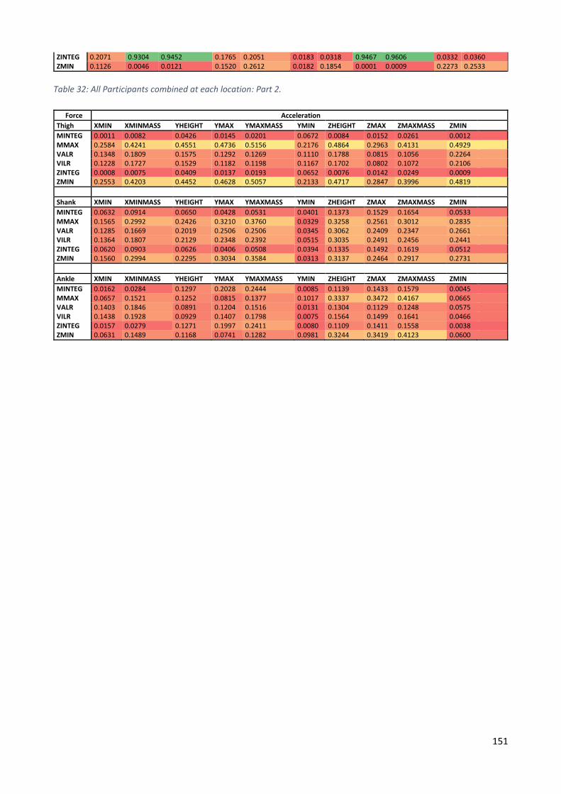
151
ZINTEG 0.2071 0.9304 0.9452 0.1765 0.2051 0.0183 0.0318 0.9467 0.9606 0.0332 0.0360 ZMIN 0.1126 0.0046 0.0121 0.1520 0.2612 0.0182 0.1854 0.0001 0.0009 0.2273 0.2533
Table 32: All Participants combined at each location: Part 2.
Force Acceleration
Thigh XMIN XMINMASS YHEIGHT YMAX YMAXMASS YMIN ZHEIGHT ZMAX ZMAXMASS ZMIN
MINTEG 0.0011 0.0082 0.0426 0.0145 0.0201 0.0672 0.0084 0.0152 0.0261 0.0012 MMAX 0.2584 0.4241 0.4551 0.4736 0.5156 0.2176 0.4864 0.2963 0.4131 0.4929 VALR 0.1348 0.1809 0.1575 0.1292 0.1269 0.1110 0.1788 0.0815 0.1056 0.2264 VILR 0.1228 0.1727 0.1529 0.1182 0.1198 0.1167 0.1702 0.0802 0.1072 0.2106 ZINTEG 0.0008 0.0075 0.0409 0.0137 0.0193 0.0652 0.0076 0.0142 0.0249 0.0009 ZMIN 0.2553 0.4203 0.4452 0.4628 0.5057 0.2133 0.4717 0.2847 0.3996 0.4819
Shank XMIN XMINMASS YHEIGHT YMAX YMAXMASS YMIN ZHEIGHT ZMAX ZMAXMASS ZMIN
MINTEG 0.0632 0.0914 0.0650 0.0428 0.0531 0.0401 0.1373 0.1529 0.1654 0.0533 MMAX 0.1565 0.2992 0.2426 0.3210 0.3760 0.0329 0.3258 0.2561 0.3012 0.2835 VALR 0.1285 0.1669 0.2019 0.2506 0.2506 0.0345 0.3062 0.2409 0.2347 0.2661 VILR 0.1364 0.1807 0.2129 0.2348 0.2392 0.0515 0.3035 0.2491 0.2456 0.2441 ZINTEG 0.0620 0.0903 0.0626 0.0406 0.0508 0.0394 0.1335 0.1492 0.1619 0.0512 ZMIN 0.1560 0.2994 0.2295 0.3034 0.3584 0.0313 0.3137 0.2464 0.2917 0.2731
Ankle XMIN XMINMASS YHEIGHT YMAX YMAXMASS YMIN ZHEIGHT ZMAX ZMAXMASS ZMIN
MINTEG 0.0162 0.0284 0.1297 0.2028 0.2444 0.0085 0.1139 0.1433 0.1579 0.0045 MMAX 0.0657 0.1521 0.1252 0.0815 0.1377 0.1017 0.3337 0.3472 0.4167 0.0665 VALR 0.1403 0.1846 0.0891 0.1204 0.1516 0.0131 0.1304 0.1129 0.1248 0.0575 VILR 0.1438 0.1928 0.0929 0.1407 0.1798 0.0075 0.1564 0.1499 0.1641 0.0466 ZINTEG 0.0157 0.0279 0.1271 0.1997 0.2411 0.0080 0.1109 0.1411 0.1558 0.0038 ZMIN 0.0631 0.1489 0.1168 0.0741 0.1282 0.0981 0.3244 0.3419 0.4123 0.0600

152
Appendix B. Logarithmic Correlations
Logarithmically modelling the vertical force and axial acceleration of all participants and for the
cohort from the generalised models.
Table 33: Participant-modelled logarithmic results.
Results of Logarithmic Modelling
Participant Location Correlation 𝑹𝟐 𝑹𝑴𝑺𝑬 (𝑵)
Force Acceleration Linear Log Linear Log
P4
Thigh
ZMIN XMAX 0.17 0.12 879.9 903.7
ZMIN XMIN 0.52 0.43 672.5 726.6
ZMIN XHEIGHT 0.36 0.31 774.7 804.9
Shank
ZMIN XMAX 0.79 0.59 445.5 619.3
ZMIN XMIN 0.47 0.44 699.0 722.8
ZMIN XHEIGHT 0.73 0.62 504.6 593.9
Ankle
ZMIN XMAX 0.17 0.22 884.6 857.2
ZMIN XMIN 0.02 0.04 957.2 947.4
ZMIN XHEIGHT 0.12 0.16 908.5 889.7
P3
Thigh
ZMIN XMAX 0.33 0.40 500.6 471.6
ZMIN XMIN 0.58 0.57 397.7 400.2
ZMIN XHEIGHT 0.52 0.55 422.2 411.2
Shank
ZMIN XMAX 0.48 0.56 431.6 397.3
ZMIN XMIN 0.13 0.14 560.2 556.1
ZMIN XHEIGHT 0.54 0.52 407.3 416.9
Ankle
ZMIN XMAX 0.09 0.08 582.5 585.2
ZMIN XMIN 0.21 0.23 540.6 535.0
ZMIN XHEIGHT 0.16 0.20 557.5 545.2
P2
Thigh
ZMIN XMAX 0.21 0.15 463.4 479.1
ZMIN XMIN 0.21 0.23 461.6 455.6
ZMIN XHEIGHT 0.25 0.25 451.0 449.7
Shank
ZMIN XMAX 0.33 0.30 415.4 426.5
ZMIN XMIN 0.32 0.33 419.7 415.9
ZMIN XHEIGHT 0.38 0.38 399.3 401.0
Ankle
ZMIN XMAX 0.21 0.19 451.4 458.4
ZMIN XMIN 0.25 0.27 440.7 434.2
ZMIN XHEIGHT 0.27 0.29 433.8 430.1
P1
Thigh
ZMIN XMAX 0.22 0.24 449.0 443.1
ZMIN XMIN 0.23 0.23 445.5 446.3
ZMIN XHEIGHT 0.33 0.33 414.6 415.3
Shank
ZMIN XMAX 0.49 0.52 356.2 345.7
ZMIN XMIN 0.01 0.02 497.3 492.7
ZMIN XHEIGHT 0.35 0.30 402.4 417.4
Ankle
ZMIN XMAX 0.54 0.55 341.3 337.4
ZMIN XMIN 0.11 0.12 476.1 471.8
ZMIN XHEIGHT 0.42 0.36 384.9 402.5

153
Table 34: Cohort-modelled logarithmic results.
Results of Logarithmic Cohort Modelling
Participant Location
Correlation R^2 RMSE (N)
Force Acceleration Linear Log Adjusted
Log Linear Log
Adjusted Log
1
Thigh
ZMIN XMAXMASS 0.29 0.16 0.12 601 650 665
ZMIN XMINMASS 0.42 0.36 0.01 541 567 708
ZMIN XHEIGHT 0.32 0.29 0.40 584 600 551
Shank
ZMIN XMAXMASS 0.59 0.39 0.29 449 552 593
ZMIN XMINMASS 0.30 0.27 0.00 589 602 702
ZMIN XHEIGHT 0.50 0.41 0.42 498 539 537
Ankle
ZMIN XMAXMASS 0.26 0.16 0.13 611 647 662
ZMIN XMINMASS 0.16 0.17 0.00 651 646 707
ZMIN XHEIGHT 0.19 0.20 0.31 637 635 589
2
Thigh
ZMIN XMAXMASS 0.29 0.16 0.19 601 650 638
ZMIN XMINMASS 0.42 0.36 0.41 541 567 546
ZMIN XHEIGHT 0.32 0.29 0.41 584 600 543
Shank
ZMIN XMAXMASS 0.59 0.39 0.40 449 552 544
ZMIN XMINMASS 0.30 0.27 0.28 589 602 598
ZMIN XHEIGHT 0.50 0.41 0.47 498 539 513
Ankle
ZMIN XMAXMASS 0.26 0.16 0.20 611 647 634
ZMIN XMINMASS 0.16 0.17 0.25 651 646 611
ZMIN XHEIGHT 0.19 0.20 0.32 637 635 586
3
Thigh
ZMIN XMAXMASS 0.29 0.16 0.19 601 650 640
ZMIN XMINMASS 0.42 0.36 0.41 541 567 544
ZMIN XHEIGHT 0.32 0.29 0.41 584 600 546
Shank
ZMIN XMAXMASS 0.59 0.39 0.40 449 552 546
ZMIN XMINMASS 0.30 0.27 0.28 589 602 597
ZMIN XHEIGHT 0.50 0.41 0.49 498 539 505
Ankle
ZMIN XMAXMASS 0.26 0.16 0.19 611 647 636
ZMIN XMINMASS 0.16 0.17 0.25 651 646 611
ZMIN XHEIGHT 0.19 0.20 0.31 637 635 587
4
Thigh
ZMIN XMAXMASS 0.29 0.16 0.24 601 650 619
ZMIN XMINMASS 0.42 0.36 0.23 541 567 623
ZMIN XHEIGHT 0.32 0.29 0.41 584 600 546
Shank
ZMIN XMAXMASS 0.59 0.39 0.44 449 552 528
ZMIN XMINMASS 0.30 0.27 0.21 589 602 627
ZMIN XHEIGHT 0.50 0.41 0.52 498 539 489
Ankle
ZMIN XMAXMASS 0.26 0.16 0.26 611 647 611
ZMIN XMINMASS 0.16 0.17 0.19 651 646 636
ZMIN XHEIGHT 0.19 0.20 0.31 637 635 589