Embed Size (px)
Citation preview

Finite Volume Solution of Two-Step Hyperbolic Conduction in Casting Sand
S. Han
Department of Mechanical Engineering
Tennessee Tech University
Cookeville, TN 38505, USA
Key words: Finite volume method, non-Fourier conduction, casting sand
Accepted for publication in Int. J. Heat and Mass Transfer, Oct. 27, 2015
1
Abstract
Finite volume method is applied for the solution of two-step hyperbolic conduction equations to
describe the short time transient heat conduction through casting sand when two energy
carriers (sand and air) are not in thermal equilibrium. Numerical results show favorable
agreement with the existing experimental data.
Nomenclature
A= bulk cross section area (m-2)
C = bulk heat capacity (Jm-3K-1)
CE = equivalent thermal wave speed (ms-1) defined by Eqn. (7c)
c= wave speed in bulk media
E= error threshold defined by Eqn. (20)
G = sand-air coupling factor (Wm-3K-1)
L = thickness (m)
q = heat flux through air (Wm-2)
qs = wall heat flux (Wm-2)
R= radius of sand grain (m)
t = time (s)
ts = wall heat flux duration time (s)
T = temperature (K)
x = spatial coordinate (m)
2

Greek Symbols
α = bulk thermal diffusivity (m2s-1)
αE= equivalent thermal diffusivity defined by Eqn. (7c)
ε =emissivity of sand
σ = Stefan-Boltzmann constant (5.670x10⁻⁸ Wm-2K-4)
γ= fraction of sand grain surface in contact with air
κ = bulk thermal conductivity (Wm-1K-1)
τ=heat flux lagging constant for bulk media (s)
τ q , τT = defined in DPL model, Eqn. (7b)
∅= void fraction
∆ t=¿ time step (s)
Subscripts
a= air
c= characteristic value
s = sand
Superscripts
1, 0, and -1 = time level at t+∆ t , t, and t−∆t , respectively
* = guessed value at t+∆ t
1. Introduction
Two step heat conduction models have been used successfully to describe fast transient of
thin metals subject to short pulse irradiation on metal surface. In these classes of models, non-
3

equilibrium thermal conditions among two energy carriers, electron and lattice are assumed.
Energy transfer first occurs to the electrons and then subsequent energy transfer from the
electron occurs to the lattice through coupling process called thermalization. Depending on
the magnitude of energy deposition time and thermalization time, non-Fourier conduction in
terms of heat flux lagging can play an important role [1, 2, and 3].
Heat transfer through porous media during a short time interval (in millisecond) shows
non-Fourier behavior as well [4]. Like laser heating of metals, the energy deposition to the air
and subsequent energy exchange between air and sand grains are considered in this approach.
Two-step models use separate temperatures for the air and sand and energy transfer between
them occurs through thermalization process. The aim of the present study is to present an
application of a finite volume method for non-Fourier conduction in casting sand as shown in
Fig. 1.
2. Heat Transfer Equations
2.1 One step model
Heat transfer equation in porous media is often expressed in terms of effective (bulk)
specific heat and conductivity of the media using void fraction which is the fraction of gas
volume in the media. In the absence of convection and energy generation, temperature of air
and sand are in thermal equilibrium and the conduction equation for the bulk media can be
expressed by [5],
C ∂T∂t
=−∂∂ x
q (1a)
q+τ ∂q∂ t
=−κ ∂T∂ x (1b)
The average volume specific heat (C=ρ c p ¿and conductivity (κ ¿of the porous media are
approximated by [6],
C=∅Ca+(1−∅ )C s;κ=∅ κ a+(1−∅ ) κ s (1c)
4

where ∅=Aa
A is the void fraction and τ is the heat flux lagging constant due to inertia effects
of aggregated porous media.
Eliminating heat flux, q , between Eqns. (1a) and (1b), hyperbolic-one-step (HOS) model
known as the Cattaneo-Vernotte (CV) equation is obtained [7].
C ∂T∂t
= ∂∂ x (κ ∂T
∂x )−τC ∂2T∂ t 2 + ∂q
∂ t∂ τ∂x
(2)
The last term in the RHS of Eq. (2) disappears in homogeneous medium. Numerous analytical
and numerical methods have been used for its solutions [8]. The most distinct feature of the
HOS model is the capability to capture sharp thermal wave front that propagates with finite
wave speed, c=√ ατ
, through the media.
By assuming the infinite thermal wave speed, τ=0, Eq. (2) reduces to diffusion equation
that is called parabolic-one-step (POS) model ;
C ∂T∂t
= ∂∂ x (κ ∂T
∂x ) (3)
The solution of diffusion model is often used to highlight the shortcomings of POS model for
micro-scale transient heat transfer processes.
2.2 Two-step model
In two-step model, transient temperatures of air (Ta) and sand grain (Ts) are not in thermal
equilibrium. Energy transfer occurs in two steps; first to air and subsequently from air to sand
grains. This idea is similar to the concept used for short laser pulse heating of thin metals. In
metals, heat transfer occurs to the electron first and subsequently to the lattice. Following this
concept, heat transfer processes can be described by the following set of coupled energy
equations for air and sand:
Ca
∂T a
∂ t=−∂q
∂ x−G (Ta−T s ) (4a)
5

q+ τa∂q∂ t
=−k a
∂T a
∂x(4b)
C s
∂T s
∂ t= ∂
∂x (κ s
∂T s
∂x )+G (T a−T s ) (4c)
Energy transfer is assumed to occur to the air at the boundary and subsequent energy
transfer from the air to the sand occurs through air-sand coupling (G) during thermalization
process. In Eq. (4b), τ ais the relaxation time for air in the porous media due to thermalization
process rather than the inertia effects in air molecules. This concept is different from the inertia
effects of electron in metals which is the relaxation time evaluated at the Fermi surface [1].
Sand temperature changes are due to diffusion in sand and heat transfer coupling between the
air and sand grain which acts as an energy source term for sand. This is the two-step hyperbolic
model used in this study.
Parabolic-two-step (PTS) model is obtained by neglecting τ a in Eq. (4b). Combining (4a)
and (4b), with τ a=0, parabolic conduction equation for air is obtained with energy sink term due
to thermalization process,
Ca
∂T a
∂ t= ∂
∂ x (κa
∂Ta
∂x )−G (T a−T s ) (5)
Equation for sand, Eqn. (4c), remains the same. In some PTS model, however, conduction in
the sand is also neglected [4].
C s
∂T s
∂ t=G (Ta−T s ) (6)
A well-known dual-phase-lag (DPL) model is obtained by combining (5) and (6) under the
assumption of constant thermal properties. Eliminating Ta from Eqns. (5) and (6), DPL model
shows for the sand temperature [4],
∂T s
∂t=αE
∂2T s
∂x2 −τq∂2T s
∂t 2 +αE τT∂∂ t ( ∂
2T s
∂ x2 ) (7a)
6

τ q=αE
CE2 ;τT=
α a
CE2 (7b)
where equivalent thermal diffusivity and equivalent thermal wave speed are defined as
αE=k a
ca+cs and CE=√ kaG
CaC s(7c)
Tzou [4] used DPL model to calculate non-Fourier conduction through cast sand grains
and compared with experimental data. DPL model requires the values of τ q∧τ T. These values
are not estimated by Eqn. (7b) since coupling factor is not evaluated explicitly. Rather, τ q∧τ T
are adjusted continually throughout the medium using experimental data to match the results
with experimental data.
Present analysis shows application of finite volume method for the solution of POS,
HOS, PTS and HTS models for transient heat transfer process in casting sand and compared with
experimental data reported in ref. [4].
3. Finite Volume Method
The energy equation for air is obtained by eliminating, q, between Eqns. (4a) and (4b);
Ca∂T a
∂ t= ∂
∂ x (κa∂Ta
∂x )−τ aCa∂2T a
∂ t2 −G (T a−T s )−τ aG∂∂t (T a−T s ) (8)
Eq. (8) is recast into a familiar form of conduction equation with source terms,
(Ca+τaG )∂T a
∂t= ∂
∂x (κa∂T a
∂ x )+Sc+SpT a−τ aCa∂2T a
∂ t 2 (9a)
where
Sc=GT s+τaG∂T s
∂ t; SP=−G (9b)
Finite volume equation is obtained by integrating Eqn. (9) over a finite control volume.
Integrations of LHS and first three terms in the RHS of Eqn. (9a) follow the standard
7

procedures as shown in ref. [9]. To integrate the 4th term in RHS, a second-order accurate finite
difference approximation for time derivative is used:
∂2T∂ t 2 ≈ 1
∆ t 2 (T P1 −2T P
0 +T P−1 ) (10)
For clarity of presentation subscript “a” is dropped and subscript “P” denotes air temperature
of a control volume under consideration. The superscripts, “1,” “0,” and “-1” refer to air
temperature at times t+∆ t , t, and t-+∆ t , respectively.
Collating all integrated terms, finite volume representation of Eqn. (9a) results in the
following standard form:
aPT P1 =aET E
1 +aW TW1 +b (11)
The subscript “E,” and “W” denotes east and west side control volume relative to the control
volume “P”. The coefficient aE,W , Pare:
aE ,W=κ e ,w
δx e, w;aP=aE+aW+aP
0 (1+τa∆ t )+(G τa
∆ t−SP)∆ x (12a)
In Eqn. (12a), aP0=
Ca∆ x∆ t
, and the interfacial conductivities, κ e ,w , are the harmonic mean values
of their neighboring values. The source term “b” is:
b=Sc∆ x+aP0 (2 τa
∆ t+1)T P
0 +τa∆ t
G∆x T P0−aP
0 ( τa∆ t )T P
−1 (12b)
Additional terms must be included in the source term when the medium is heterogeneous with
temperature dependent specific heat [10].
The energy equation for sand, Eq. (4c) is a parabolic equation and the finite volume
representation of Eq. (4c) is similar to Eq. (11, 12a, b) except the terms due to heat flux lagging
constant since heat transfer in the sand is assumed to be Fourier conduction.
8

The coupled energy equations for air and sand are solved by a segregated iterative
scheme. The known initial temperatures of air (T a−1 , Ta
0 ) and sand(T s0 ) and initially guessed
temperatures for air (T a1¿
) and sand(T s1¿
)are used to evaluate all coefficients and source terms in
Eq. (12a, b). Resulting simultaneous equations, Eq. (11), are solved by Thomas algorithm to
obtain the air temperature at the new time level (T a1 ). By similar method sand temperature at
the new time level (T s1) is calculated. This process continues until the air and sand temperatures
at the new time level are converged within a prescribed tolerance at all control volumes
including the boundaries:
|T a ,s1 −Ta , s
1¿
T a ,s1 |≤10−6 (13)
The accuracy of numerical results depends on time step. In the present study time step is
determined as discussed in ref. [11], which satisfies both pure diffusion and wave equation at
the initial temperature:
∆ t=0.1√τa∆ t d (14)
where ∆ t d≤∆x2
α is the time step required for explicit method for diffusion equation.
4. Estimation on Coupling Constant and Heat Flux Lagging Constant
In two-step models, heat transfer from the air to the sand grain is treated as a source
term for the sand grain, Eq. (4c). Actual heat transfer process would involve conduction and
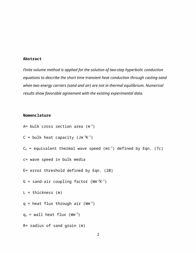
radiation in a complex geometry. To simplify the analysis, assume a spherical sand grain
surrounded by air as shown in Fig. 2. The rate of heat transfer to the sand grain from the air
through its surface in contact with air is approximated by including conduction and radiation as
dq=dA s[κ c
Lc+σε (T s
2+Ta2 ) (T s+T a )] (T a−T s ) (15a)
where κ c /Lc is the characteristic conduction conductance and dAs is the effective surface of the
sphere in heat transfer with air. It is assumed that only some fraction of sphere surface (γ ¿ is in
9

this process. Divided by the volume of sand grain, dv, energy source per unit volume of sand
grain is
dqdv
=G (T a−T s ) (15b)
For a sphere of radius R, d A s=γ (4 π R2)∧dv= 43π R3, and from (15a) and (15b), coupling
factor is given by
G=3 γR
[κc
Lc+σε (T s
2+T a2 ) (T s+Ta ) ] (16)
Actual value of γ, κ c ,∧Lc are heuristically determined.
The flux lagging time for air (τ a¿ is caused by the thermalization process. It is interpreted
as the time duration to bring the temperature of the heated air in equilibrium with the sand
temperature. From Eqn. (4c),
cs
∂T s
∂ tG (T a−T s ) (17)
Denoting the temperature before and after thermalization by superscript “0” and “1”
respectively, Eqn. (17) can be written:
τ acs
GT s
1−T s0
T a0−T s
0 (18)
Thermal equilibrium occurs whenT s1=0.5 (T a
0+T s0 ), and Eqn. (18) reduces to
τ a 0.5cs
G(19)
5. Comparison with Experimental Data
The experimental set up to measure the transient response of temperature of casting sand
with average diameter of 0.2 mm due to a short energy pulse on the surface is described in ref.
[4]. Fig. 1 shows schematics of the experimental set up. Thermocouples are located at eight
locations (0.4, 1.5, 2.1, 3.6 4.5, 5.7, 8.3, and 10.2 mm from the source of thermal pulse) and
temperature changes responding to two pulse duration of 0.14 s and 0.56 s are recorded at
these locations. The pulse power is maintained at a constant qs= 5.1 W/cm2.
10

Tzou [4] shows that diffusion model (POS) and CV wave model (HOS) cannot predict the
transient behavior at the locations near the pulse source accurately. However, DPL model
which is a special case of parabolic-two-step (PTS) model shows excellent agreement with
experimental data. To match the results, nonhomogeneous phase lags for bothτ q∧τ T, are
determined by using contour pattern of the error estimate as defined by
E (τ T , τq )=∑i=1
M
⌊T DPL (x i , ti ; τT , τq )−T exp (x i , t i ) ⌋
M(20)
At a selected location, xi, the error threshold are calculated by using measured transient
temperature and temperature predicted by DPL model for a range of τT∧τq. The optimal
values ofτT∧τq are selected that give the minimum error threshold. Results from DPL model are
shown to agree very well with the experimental data at three locations, x=0. 4 mm (
τT=4.48 s , τq=8.94 s¿ , x=1.5mm(τT=1.0 s , τ q=1.96 s) ,¿ x=2.1mm(τ ¿¿T=0.4 s , τq=0.12 s) .¿
In the present study numerical solutions using the finite volume method for POS, HOS,
PTS and HTS are obtained and compared with the experimental data. The physical properties of
sand and air used in the present analysis are listed in table 1. They may not be exactly the same
values as used in the experiment since only the bulk conductivity and the thermal diffusivity are
listed in experimental data [4].
4.1 POS model
Eqn. (3) is solved with the following initial and boundary conditions.
T ( x ,0 )=300 K (21a)
and
−κ ∂T∂ x
(0 , t )=qs for 0≤ t ≤ ts ;−κ ∂T∂ x
(0 ,t )=0 for t ≥ t s (21b)
∂T∂x
(L , t )=0
11

The bulk properties, the heat source strength and its duration are those used in ref. [4]. They
are κ = 0.29 Wm-1K-1, α=0.3 x10⁻⁶m2 s−1 ,C¿( κα )= 0.967x10⁶ Jm-3K-1, qs =5.1x10⁴ Wm-2 and
ts=0.14 s.
In numerical computation, L=0.01 m is used. This depth is large enough to ensure
adiabatic boundary condition at x=L. In all numerical results presented in this study, 400
uniform control volumes are found to be adequate to have grid independent solutions.
Fig. 3 shows transient temperature at three locations (x=0.4, 1.5 and 2.1 mm) near the surface
compared with the experimental data. POS model predicts temperature rises at x=0.4 mm (two
sand grains away) much more rapidly than the experimental data with higher peak
temperature. Similar trends are shown at x=1.5 mm. Disagreement with experimental data
becomes less severe as the distance from the surface increases. At distance far away (x≥3.6
mm), diffusion model gives satisfactory results as in ref. [4].
4.2 HOS model
HOS model, Eqn. (2), delays the response of temperature rise due to inertia effects. The
flux lagging constant τ in the 2nd term of RHS in Eqn. (2), acts initially like energy sink which
results in slower temperature rise followed by a rapid increase in temperature as the wave
passes through. Exact value of lagging constant for the bulk medium is not known. However, by
visual inspection of the temperature rise at x=0.4 mm from diffusion model, Fig. 3, its
approximate value can be estimated.
Fig. 4 shows the results corresponding to τ=0.05, and 0.1 s. At x=0.4 mm, temperature
rise in early time matches with experimental data but the maximum temperature rise is much
higher than the experimental value. These results show HOS model is not capable of predicting
transient temperature in the near field.
4.3 PTS model
In the present analysis, governing equations for PTS model are Eqn. (5) for air and Eqn.
(4c) for sand. The properties of air and sand are not given separately in the experimental data
and the porosity is also not given. Air properties at 300 K are used [12]. They are κa=0.0263
12

Wm-1K-1, and Ca =1169.5 Jm-3K-1. Sand properties are assumed to be those of bulk properties as
used for one-step models: κ s = 0.29 Wm-1K-1,α s=0.3x 10⁻⁶m2 s−1 ,C s=¿ 0.967x10⁶ Jm-3K-1 . Since
the conductivity of sand is an order of magnitude greater than air and the specific heat of sand
is three orders of magnitude greater than air, this assumption is acceptable unless the void
fraction is large.
The initial conditions are
T a ( x ,0 )=T s ( x ,0 )=300 K (22a)
The boundary conditions are given pulse heat source at x=0 for air and insulated boundary for
sand and insulated boundary for both air and sand at x=L ;
−κa
∂T a
∂ x(0 , t )=qs for0≤ t ≤ t s;−κa
∂T a
∂ x(0 , t )=0 for t ≥ ts (22b)
∂T a
∂ x(L , t )=
∂T s
∂x(L , t )=
∂T s
∂x(0 ,t )=0
In the present PTS model conductivity of sand which is much higher than air is included. For
metals, conductivity of lattice is frequently neglected since its magnitude is much smaller than
electron [2].
The coupling factor G plays an important role in PTS model. To evaluate the magnitude
of G, Eqn. (16) is used. With a choice of κ c≈κa and Lc≈ R for the conduction and ε=0.9[12],
T s=T a=300 K (initial temperature) for the radiation, and γ=0.25 ,coupling factor for 2 mm
diameter sand grain is,
G≈7.5 x 10³ (263+5.51 )=2.0 x10⁶W m−3K−1 (23)
Admittedly, this value can only represent a rough estimation but serves as a baseline value for
PTS model. Subsequent calculations with different values of G show the validity of this
approach. It is clear that radiation effects are very small unless temperature is much higher
than the initial temperature.
13

Fig. 5 shows the temperature of sand compared with the experimental data with the
baseline value of G. The results are almost identical to the results of POS model shown in Fig. 3.
To investigate the effects of G, two additional values of G are used, G=1.0x10⁶ Wm-3K-1 and
G=3.0x10⁶ Wm-3K-1. Fig. 6 shows temperature change of sand and air at x=0.4 mm. Air
temperature shows strong dependency on the coupling factor in time less than 0.2 sec. Sand
temperature dependency is rather small. With increasing value of G, temperature difference
between the air and sand decreases as expected since coupling occurs more strongly. The
effects of G are limited for a short period, less than 0.25 sec. At G=3.0x10⁶ Wm-3K-1,
temperature difference between the air and sand is very small. Increasing G value further does
not change the temperature response at x=0.4 mm. It is clear that PTS model prediction is not
much better than POS model no matter what value of coupling factor is used.
In some PTS models, conductivity of secondary energy carrier is neglected [2, 4].
However, conductivity of sand is an order of magnitude higher than air in the present case and
conductivity of sand cannot be neglected. Fig. 7 shows the results without diffusion in the sand.
Temperature increases continually at x=0.4 mm while very small energy transfer is detected at
x=1.5 mm and no transfer at all at x=2.1 mm. These results show clearly, at least in the context
of the present approach, diffusion in secondary carrier is as important as the thermalization
process.
4.4 HTS model
HTS model solves Eqn. (8) for air and Eqn. (4c) for sand. The initial and boundary
conditions are identical to PTS model except one additional initial condition for air,
∂T a
∂ t(x ,0 )=0 (24)
The lagging constant τ a is evaluated by using Eqn. (19). Using the volume specific heat of sand
and the coupling factor calculated for R=2mm sand grain, τ a 0.25 sec .
Fig. 8a shows the sand temperature predicted by HTS model with G=2.0x10⁶ Wm-3K-1
and τ a=0.25 s compared with experimental data at three locations. Agreement at x=0.4 mm is
14

much better than the results from other models. Fig. 8b shows comparison of air and sand
temperature for the case shown in Fig. 8a. Non-equilibrium condition exists in time less than
1.0 sec at x=0.4 mm. Fig. 9 shows the results of another case with G=3.0x10⁶Wm-3K-1, and
τ a=0.2 s . Shortening the lagging constant decreases response time and slightly increases higher
maximum temperature at x=0.4 mm. Otherwise results are very similar to Fig. 8a.
All the results discussed so far the heat flux pulse duration time is fixed at 0.14 s. Fig.
10a shows sand temperature with increased pulse time, ts=0.56 s with G=2.0x10⁶ Wm-3K-1 and
τ a=0.2 s. In the numerical calculation, properties of air and sand are the same values (table 1)
as used for ts=0.14s cases. But experimental data reported use bulk properties slightly different
at each location. Relatively good agreement may indicate that non-Fourier behavior is less
pronounced with increased pulse duration time. Fig. 10b shows the results with a change in
specific heat of sand from 0.967x10⁶ Wm-3K-1 to 0.87x10⁶ Wm-3K-1. All other properties remain
the same. With reduced specific heat, temperature increases higher and the results are in
excellent agreement with experimental data.
In all numerical calculations for two-step model, energy balances are taken in terms of
relative energy imbalance, defined as|qstored−q¿|/q¿, where q¿=∫0
ts
qsdt , and qstored is the energy
increase in the medium. It is less than 1.0x10⁻⁹ for PTS model and less than 1.0x10⁻⁷ for HTS
model.
6. Conclusions
A finite volume numerical method is used for the solution of non-Fourier heat conduction
in casting sand in which two energy carriers, air and sand, are not in thermal equilibrium.
Diffusion model, C-V model and parabolic-two-step models are shown to be inadequate to
describe temperature response of sand grains near the energy pulse source. Hyperbolic-two-
step model with properly chosen coupling factor and flux lagging constant for air are shown to
predict the near field behavior reasonably well.
15

The numerical method described in this study is similar to the method used for fast
transient in thin metals where electron-lattice coupling factor (G) and electron heat flux
lagging constant (τ F ¿ are given physical properties of metals [10]. In the present study,
however, coupling factor (G) and flux lagging constant for gas in porous media are estimated
by a simplified heat transfer model between the gas and solid materials. It is shown that
coupling factor is inversely proportional to the radius of sand grain while flux lagging constant
is proportional to its radius.
Acknowledgement
The author is grateful to the reviewers for comments that made the paper more clear
and balanced.
References
1. T. Q. Qui and C. L. Tien, Heat transfer mechanisms during short-pulse laser heating
of metals, J. Heat transfer, 115, 835-841 (1993).
2. T. Q. Qui and C. L. Tien, Femtosecond laser heating of multi-layer metals – I. Analysis,
Int. J. Heat Mass Trans., 37, No. 17, 2789-2797 (1994).
3. L. Jiang and H. L. Tsai, Improved two–temperature model and its application in
ultrashort laser heating of thin films, J Heat Transfer, 127, 1167-1173 (2005).
4. D. Y. Tzou, Macro-to-Microscale Heat transfer, Chap. 6, Taylor & Francis,
Washington, DC (1997).
5. M. J. Mauer, Relaxation model for heat conduction in metals, J. Appl. Phys., 40,
5123 -5130 (1969).
6. A. Bejan, Convection Heat Transfer, Chap. 10, Wiley & Sons, New York (1984).
16

7. C. Cattaneo, A form of heat conduction equation which eliminates the paradox of
instantaneous propagation, Compte Rendus, 247, 431-433 (1958).
8. D. Y. Tzou, Computational techniques for microscale heat transfer, 2nd ed., W. J.
Minkowycz, E. M. Sparrow, and J. Y. Murthy, eds., Wiley, Hoboken, NJ (2006).
9. S. V. Patankar, Numerical Heat Transfer and Fluid Flow, McGraw-Hill, New York, NY,
(1980).
10. S. Han, Finite volume solution of a hyperbolic two-step conduction equation,
Numerical Heat transfer, Part A, 68: 1050-1066, (2015a).
11. S. Han, Finite volume solution of a 1-D hyperbolic conduction equation, Numerical
Heat Transfer, Part A, 67: 497-512, (2015b).
12. F. P. Incropera, D. P. Dewitt, T. L. Bergman and A. A. Lavine, Fundamentals of Heat
and Mass Transfer, Appendix A, Wiley & Sons, 6th ed., New York (2007).
Table captions
Table 1 Properties of air and sand
17

Bulk conductivity (κ )1 0.290 Wm-1K-1
Bulk thermal diffusivity (α )1 0.3x10⁻⁶ m2s-1
Thermal conductivity of air (κa )2 0.0263 Wm-1K-1
Thermal conductivity of sand (κ s )3 0.290 Wm-1K-1
18

Specific heat of air (Ca )2 1169 Jm-3K-1
Specific heat of sand (C s )3 0.967x10⁶ Jm-3K-1
1. Ref. [4]2. Ref. [12], at 300 K3. Assuming very small void fraction, ϕ≪1
Table 1
Figure captions
Fig. 1 Schematics of constant heat flux impinging on the surface of porous media (casting sand ) of
thickness L
Fig. 2 Simplified planar view of a sand grain surrounded by air
19

Fig. 3 Comparison of transient sand temperature: POS model (solid line) with experimental data at
X=0.4mm (o), x=1.5 mm (x), and x=2.1 mm (*); ts=0.14 s, qs=5.1 x10⁴ Wm-2
Fig. 4 Comparison of transient sand temperature: HOS model (solid line) with experimental data at
X=0.4mm (o), x=1.5 mm (x), and x=2.1 mm (*); ts=0.14 s, qs=5.1 x10⁴ Wm-2;
τ=0.05 s (a) , τ=0.1 s(b)
Fig. 5 Comparison of transient sand temperature: PTS model (solid line) with experimental data at
X=0.4mm (o), x=1.5 mm (x), and x=2.1 mm (*); ts=0.14 s, qs=5.1 x10⁴ Wm-2; G=2.0x10⁶ Wm-3K-1
Fig. 6 (a) Transient air temperature and (b) transient sand temperature at x=0.4 mm predicted by PTS
model with different G values: G=1.0x10⁶ (broken line), G=2.0x10⁶ (solid line) and G=3.0x10⁶
Wm-3K-1 (O); ts=0.14 s, qs=5.1 x10⁴ Wm-2
Fig. 7 Comparison of transient sand temperature: PTS model with κ s=0 (solid line) with experimental
data at X=0.4mm (o), x=1.5 mm (x), and x=2.1 mm (*); ts=0.14 s, qs=5.1 x10⁴ Wm-2; G=2.0x10⁶
Wm-3K
Fig. 8 (a ) Comparison of transient sand temperature: HTS model (solid line) with experimental data at
X=0.4mm (o), x=1.5 mm (x), and x=2.1 mm (*) and (b) comparison of air (broken line) and sand
temperature (solid line); ts=0.14 s, qs=5.1 x10⁴ Wm-2; τ a=0.25 s ,∧¿G=2.0 x10⁶ Wm-3K-1
Fig. 9 Comparison of transient sand temperature: HTS model (solid line) with experimental data at
X=0.4mm (o), x=1.5 mm (x), and x=2.1 mm (*); ts=0.14 s, qs=5.1 x10⁴ Wm-2; τ a=0.20 s ,∧¿
G=3.0 x10⁶ Wm-3K-1
Fig. 10 Comparison of transient sand temperature: HTS model (solid line) with experimental data at
X=0.4mm (o), x=1.5 mm (x), and x=2.1 mm (*); (a) Cs =0.967x10⁶ Jm-3K-1 and (b) Cs =0.87x10⁶
Jm-3K-1 ; ts=0.56 s, qs=5.1 x10⁴ Wm-2; τ a=0.20 s ,∧¿G=2.0 x10⁶ Wm-3K-1
20

21casting sand
qs

Fig.1
22
air
sand

Fig.2
23

0 1 2 3 4 50
1
2
3
4
5
6
7
8
9
10
time (s)
Tem
pera
ture
chan
ge (K
)
pulse width: 0.14 s diffusion (POS)
Fig. 3
24

0 0.5 1 1.5 2 2.5 3 3.5 4 4.5 50
2
4
6
8
10
12
time (s)
Tem
pera
ture
cha
nge
(K)
pulse width: 0.14 s
CV wave (HOS)
(a)
0 1 2 3 4 50123456789
101112
time (s)
Tem
pera
ture
chan
ge (K
)
pulse width : 0.14 s CV wave (HOS)
(b)
Fig. 4a, b
25

0 0.5 1 1.5 2 2.5 3 3.5 4 4.5 50
1
2
3
4
5
6
7
8
9
time (s)
Tem
pera
ture
chan
ge (K
)
PTS Sand temperature G=2.0e6
Fig. 5
26

0 0.1 0.2 0.3 0.4 0.5 0.6 0.7 0.8 0.9 10
5
10
15
20
25
30
35
time (s)
Air t
empe
ratu
re ch
ange
(K)
PTS air temperature at x=0.4 mm
G=1.0e6
G=2.0e6
G=3.0e6
(a)
0 0.1 0.2 0.3 0.4 0.5 0.6 0.7 0.8 0.9 10
1
2
3
4
5
6
7
8
9
time (s)
Sand
tem
pera
ture
chan
ge (K
)
G=1.0e6
G=2.0e6
G=3.0e6
sand temperature at x=0.4 mm
(b)
Fig. 6a, b
27

0 0.5 1 1.5 2 2.5 3 3.5 4 4.5 50
1
2
3
4
5
6
7
8
9
time (s)
Tem
pera
ture
chan
ge (K
)
PTS G=2.0e6
Fig. 7
28

0 1 2 3 4 5 60
1
2
3
4
5
6
7
8
time (s)
Tem
pera
ture
chan
ge (K
)
HTS sand temperature
G=2.0e6 pulse width = 0.14 s
(a)
0 0.5 1 1.5 2 2.5 3 3.5 4 4.5 50
1
2
3
4
5
6
7
8
9
time (s)
Tem
pera
ture
chan
ge (K
)
HTS
G=2.0e6pulse width=0.14 sAir sand
(b)
Fig. 8a, b
29
0 0.5 1 1.5 2 2.5 3 3.5 4 4.5 50
1
2
3
4
5
6
7
8
time (s)
Tem
pera
ture
chan
ge (K
)
HTSsand temperature
G=3.0e6pulse width =0.14 s
Fig. 9
30

0 2 4 6 8 10 12 140
5
10
15
20
25
30
35
time (s)
Tem
pera
ture
chan
ge (K
)
(a)
0 2 4 6 8 10 12 140
5
10
15
20
25
30
35
time (s)
Tem
pera
ture
chan
ge (K
)
HTSpulse duration=0.56 s
G=2.0e6
(b)
Fig. 10a, b
31


![Web viewHeat Pump Type [Choose an item]](https://img.pdfslide.us/doc/110x75/5a7048377f8b9aa7538bdd97/wwwhydrombca-nbspdoc-fileweb-viewheat-pump-type.jpg)