Embed Size (px)
Citation preview

Shallow water equations in channel networks
Maya Briani
Istituto per le Applicazioni del Calcolo “M. Picone”Consiglio Nazionale delle Ricerche
http://www.iac.rm.cnr.it/∼briani
May 5 - 2021
Maya Briani (IAC-CNR) Shallow water equations in channel networks May 5 - 2021 1 / 42

Plan of the talk
(1) The Shallow Water Equations
(2) The Riemann Problem
(3) Water Flow in Canal Network
(4) The Junction Riemann Problem
(5) Fluvial to torrential transition
(6) Conclusions and Open Problems
Maya Briani (IAC-CNR) Shallow water equations in channel networks May 5 - 2021 2 / 42

The Shallow Water Equations
The Shallow Water Equations
The one-dimensional shallow water equations describe the waterpropagation in a canal with rectangular cross-section and constant slope:
∂th+ ∂x(hv) = 0 conservation of mass
∂t(hv) + ∂x(hv2 + 1
2gh2) = 0 conservation of momentum
(1)
I h(x, t) the water height
I v(x, t) the water velocity at time t and location x along the canal
I g the gravity constant
For the purpose of this talk, we have assumed a steady state friction on allcanals and horizontal canals with zero slope.
Maya Briani (IAC-CNR) Shallow water equations in channel networks May 5 - 2021 3 / 42

The Shallow Water Equations
The Shallow Water Equations
We reformulate system (1) in vector form as
∂tu+ ∂xf(u) = 0 (2)
where
u =
(hq
)f(u) =
(hv
hv2 + 12gh
2
)(3)
and q = hv (discharge, it measures the flow rate of water past a point).
The Riemann Problem∂tu+ ∂xf(u) = 0,
u(x, 0) =
{ul if x < 0,ur if x > 0.
(4)
Here u(x, 0) = (h(x, 0), q(x, 0)) and ul = (hl, ql) and ur = (hr, qr).
Maya Briani (IAC-CNR) Shallow water equations in channel networks May 5 - 2021 4 / 42

The Riemann Problem for shallow water equations
The Riemann Problem
x
t
0
l-wave r-waveu∗
ul ur↗ ↖
Figure: The solution to the Riemann problem. The intermediate state u∗ is constant in theregion delimited by l-wave and r-wave. l- and r-waves are shocks or rarefactions.
I The solution to this Riemann problem consists of the l-wave and the r-waveseparated by an intermediate state u∗ = (h∗, q∗).
I This intermediate state is connected to ul = (hl, ql) through a physicallycorrect l-waves, and to ur = (hr, qr) through a physically correct r-wave.
Maya Briani (IAC-CNR) Shallow water equations in channel networks May 5 - 2021 5 / 42

The Riemann Problem for shallow water equations
The Shallow Water Equations - The Riemann Problem
For smooth solution, system (2) can equivalently be written in thequasilinear form
∂tu+A(u)∂xu = 0where the Jacobian matrix A(u) = f ′(u) is
A(u) =
(0 1
−v2 + gh 2v
)The eigenvalues of the matrix A(u) are
λ1(u) = v −√gh, λ2(u) = v +
√gh
with the corresponding eigenvectors r1(u) = (1, v +√gh)T and
r2(u) = (1, v +√gh).
Maya Briani (IAC-CNR) Shallow water equations in channel networks May 5 - 2021 6 / 42

The Riemann Problem for shallow water equations
The Riemann Problem
I The shallow water equations are genuinely nonlinear (∇λj(u) · rj(u) 6= 0,j = 1, 2) and so the Riemann problem always consists of two waves, each ofwhich is a shock or rarefaction.
I The left and right characteristics are associated to λ1 and λ2 respectively.
I λ1 = v −√gh and λ2 = v +
√gh can be of either sign.
I The ratio Fr = |v|/√gh is called the Froude number.
I When v = q/h is smaller than the speed√gh of the gravity waves:
|v| <√gh or Fr < 1
the fluid is said to be fluvial or subcritical.
If |v| >√gh the fluid is said to be torrential or supercritical.
I Under the fluvial regimeλ1 < 0 λ2 > 0
and there will be one left (with negative speed) and one right (with positivespeed) going wave.
Maya Briani (IAC-CNR) Shallow water equations in channel networks May 5 - 2021 7 / 42

The Riemann Problem for shallow water equations
The solution always consists of two waves, each of which is a shock orrarefaction:
(R) Centered Rarefaction Waves. Assume u+ lies on the positivei-rarefaction curve through u−, then we get
u(x, t) =
u− for x < λi(u
−)t,Ri(x/t;u
−) for λi(u−)t ≤ x ≤ λi(u+)t,
u+ for x > λi(u+)t,
(S) Shocks. Assume that the state u+ is connected to the right of u− byan i-shock, then calling λ = λi(u
+, u−) the Rankine-Hugoniot speedof the shock, the function
u(x, t) =
{u− if x < λtu+ if x > λt
provides a the solution to the Riemann problem. For strictlyhyperbolic systems, we have that
λi(u+) < λ(u−, u+) < λi(u
−), λ(u−, u+) =q+ − q−
h+ − h−.
Maya Briani (IAC-CNR) Shallow water equations in channel networks May 5 - 2021 8 / 42

The Riemann Problem for shallow water equations
The Riemann Problem - Lax curves
To find the intermediate state u∗ in general we can define two functions φland φr by
φl(h) =
{vl − 2(
√gh−
√ghl) if h < hl (rarefaction)
vl − (h− hl)√g h+hl2hhl
if h > hl (shock wave),
and
φr(h) =
{vr + 2(
√gh−
√ghr) if h < hr (rarefaction)
vr + (h− hr)√g h+hr2hhr
if h > hr (shock wave).
For a given state h
I the function φl(h) returns the value of v such that (h, hv) can be connectedto ul by a physically correct l-wave
I the function φr(h) returns the value of v such that (h, hv) can be connectedto ur by a physically correct r-wave.
I So, h∗ is such that φl(h∗) = φr(h
∗)
Maya Briani (IAC-CNR) Shallow water equations in channel networks May 5 - 2021 9 / 42

The Riemann Problem for shallow water equations
The Riemann Problem
h
0 1 2 3 4 5 6 7
v
-10
-5
0
5
10
15
λ1 < 0 λ2 > 0
uluru∗
φl
Rl
Sl
φrSr
Rr
Maya Briani (IAC-CNR) Shallow water equations in channel networks May 5 - 2021 10 / 42

The Riemann Problem for shallow water equations
Example: Dam-Break and Riemann Problem
Consider the Riemann problem with
ul =
(hlql
)=
(10
)ur =
(hrqr
)=
(0.50
).
I hl > hr and ql = qr = 0. This Riemann problem models what happens in adam separating two levels of water breaks at time t = 0
I The solution consists of a l-rarefaction and a r-shock
0 0.1 0.2 0.3 0.4 0.5 0.6 0.7 0.8 0.9 1
x
0
0.2
0.4
0.6
0.8
1
h
0 0.1 0.2 0.3 0.4 0.5 0.6 0.7 0.8 0.9 1
x
0
0.2
0.4
0.6
0.8
1
q
Maya Briani (IAC-CNR) Shallow water equations in channel networks May 5 - 2021 11 / 42
Water Flow in a Channel Network
Water Flow in a Canal Network
Maya Briani (IAC-CNR) Shallow water equations in channel networks May 5 - 2021 12 / 42
Water Flow in a Channel Network
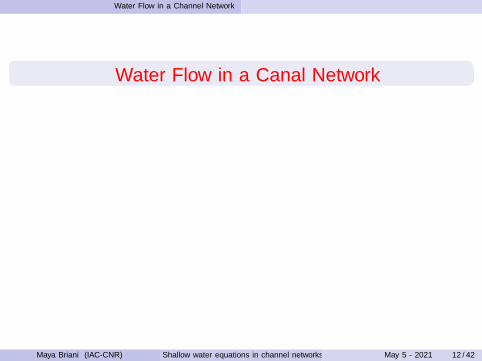
Water Flow in a Channel Network
−→
JCanal 1
Canal 2
Canal 3On each canal
∂tui + ∂xf(ui) = 0
?y#
Maya Briani (IAC-CNR) Shallow water equations in channel networks May 5 - 2021 13 / 42

Water Flow in a Channel Network
Water Flow in a Channel Network
−→
JCanal 1
Canal 2
Canal 3On each canal
∂tui + ∂xf(ui) = 0
?y#
Maya Briani (IAC-CNR) Shallow water equations in channel networks May 5 - 2021 13 / 42

Water Flow in a Channel Network
Water Flow in a Channel Network
−→
JCanal 1
Canal 2
Canal 3On each canal
∂tui + ∂xf(ui) = 0
?y#
Maya Briani (IAC-CNR) Shallow water equations in channel networks May 5 - 2021 13 / 42

Water Flow in a Channel Network
Water Flow in a Channel Network
−→
JCanal 1
Canal 2
Canal 3On each canal
∂tui + ∂xf(ui) = 0
unknowns:
u∗1 = (h∗1, q
∗1)
u∗2 = (h∗2, q∗2)
u∗3 = (h∗3, q∗3)y
#
Maya Briani (IAC-CNR) Shallow water equations in channel networks May 5 - 2021 14 / 42

Water Flow in a Channel Network
Water Flow in a Channel Network
−→
JCanal 1
Canal 2
Canal 3On each canal
∂tui + ∂xf(ui) = 0
Conservation of mass
Junction Riemann Problem
Closure conditionsy#
Maya Briani (IAC-CNR) Shallow water equations in channel networks May 5 - 2021 15 / 42

Water Flow in a Channel Network
Water Flow in Canal Network: 1-to-2 Junction
Assuming that the three canals are connected at x = 0:
Canal 1 (x < 0)
∂tu1 + ∂xf(u1) = 0
Canal 2 and 3 (x > 0)
∂tu2 + ∂xf(u2) = 0
∂tu3 + ∂xf(u3) = 0
Assuming the conservation of mass
q∗1(0−, t) = q∗2(0
+, t) + q∗3(0+, t)
To get a well-posed problem we need 5 additional conditions
Maya Briani (IAC-CNR) Shallow water equations in channel networks May 5 - 2021 16 / 42

Water Flow in a Channel Network
The Junction Riemann Problem
The solution is determined once one assigns a Riemann Solver at thejunction. Considering only subcritical states
I given constant initial conditions (u0i , u0j ) (i ranges over incoming
canals, j over outgoing ones);
I the Junction Riemann solution consists of intermediate states (u∗i , u∗j )
satisfying some other junction conditions
x
t
0
l-wave r-wave
u0i u0j
u∗i u∗j↗ ↖←→
junction conditions
Maya Briani (IAC-CNR) Shallow water equations in channel networks May 5 - 2021 17 / 42

Water Flow in a Channel Network
Left-half Riemann Problem (the case of an incoming canal)
We fix a left state and we look for the right states attainable by waves ofnegative speed. ⇒ Fix ul = (hl, ql), we look for the set of pointsu∗l = (h∗l , q
∗l ) such that the solution to the Riemann problem
∂tu+ ∂xf(u) = 0,
u(x, 0) =
{ul if x < 0u∗l if x > 0
contains only waves with negative speed (λ1(u∗l ) < 0).
x
t
0
l-wave
ul
u∗l↗
0 1 2 3 4 5 6 7
h
-10
-5
0
5
10
15
v
φl
ul
λ1 < 0
Maya Briani (IAC-CNR) Shallow water equations in channel networks May 5 - 2021 18 / 42
Water Flow in a Channel Network
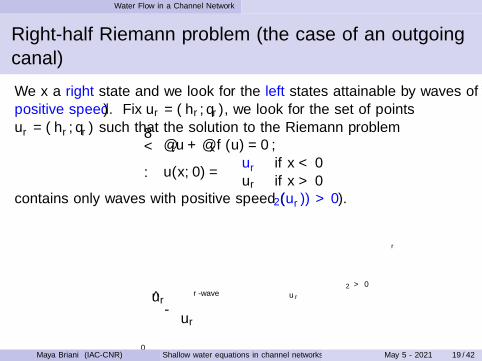
Right-half Riemann problem (the case of an outgoingcanal)
We fix a right state and we look for the left states attainable by waves ofpositive speed.⇒ Fix ur = (hr, qr), we look for the set of pointsu∗r = (h∗r , q
∗r ) such that the solution to the Riemann problem
∂tu+ ∂xf(u) = 0,
u(x, 0) =
{u∗r if x < 0ur if x > 0
contains only waves with positive speed (λ2(u∗r)) > 0).
x
t
0
r-wave
ur
ur↖
0 1 2 3 4 5 6 7
h
-10
-5
0
5
10
15
v
φr
ur
λ2 > 0
Maya Briani (IAC-CNR) Shallow water equations in channel networks May 5 - 2021 19 / 42

Water Flow in a Channel Network
The Junction Riemann Problem
0 1 2 3 4 5 6 7
h
-10
-5
0
5
10
15
v
φl
ul
λ1 < 0
0 1 2 3 4 5 6 7
h
-10
-5
0
5
10
15
v
φr
ur
λ2 > 0
v∗l = φl(h∗l ;hl, vl) v∗r = φr(h
∗r ;hr, vr)
|v∗l,r| <√gh∗l,r
Maya Briani (IAC-CNR) Shallow water equations in channel networks May 5 - 2021 20 / 42
Water Flow in a Channel Network
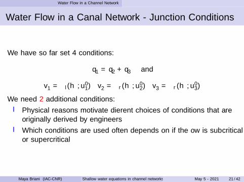
Water Flow in a Canal Network - Junction Conditions
We have so far set 4 conditions:
q∗1 = q∗2 + q∗3 and
v∗1 = φl(h∗;u01) v∗2 = φr(h
∗;u02) v∗3 = φr(h∗;u03)
We need 2 additional conditions:
I Physical reasons motivate different choices of conditions that areoriginally derived by engineers
I Which conditions are used often depends on if the flow is subcriticalor supercritical
Maya Briani (IAC-CNR) Shallow water equations in channel networks May 5 - 2021 21 / 42

Water Flow in a Channel Network
Water Flow in Canal Network - Junction Conditions
The conservation of mass is usually coupled with the following:
I Equal water pressure (equal water heights)
1
2gh2k =
1
2gh2l ∀t > 0
I Energy continuity (equal of energy levels)
hk +v2k2g
= hl +v2l2g
∀t > 0
Other conditions which depend on the geometry:I Preprint 2021 M. Briani, G. Puppo, M. Ribot, Angle dependence incoupling conditions for shallow water equations at canal junctions
Maya Briani (IAC-CNR) Shallow water equations in channel networks May 5 - 2021 22 / 42

Water Flow in a Channel Network
Water Flow in a Channel Network
−→
On each canal∂tui + ∂xf(ui) = 0
h∗1 = h∗
2 = h∗3 = h∗,
v∗1 = v∗2 + v∗3,
v∗1 = φl(h∗;u0
1),
v∗2 = φr(h∗;u0
2),
v∗3 = φr(h∗;u0
3),
|v∗k| <√gh∗
#
starting by Riemann data
u1(J−) = u01, u2(J
+) = u02, u3(J+) = u03.
Maya Briani (IAC-CNR) Shallow water equations in channel networks May 5 - 2021 23 / 42

Water Flow in a Channel Network
The Junction Riemann Problem
The solution at the Junction then consists on solving the non-linearsystem
h∗1 = h∗2 = h∗3 = h∗,
v∗1 = v∗2 + v∗3,
v∗1 = φl(h∗;u01),
v∗2 = φr(h∗;u02),
v∗3 = φr(h∗;u03),
(5)
with h∗ > 0 and the subcritical assumption |v∗k| <√gh∗, k = 1, 2, 3
I the system admits a unique solution (see for instance Marigo 2010)... but the solution not always verifies the subcritical condition
I suitable initial data have to be given to ensure the fluvial regime tothe problem.
Maya Briani (IAC-CNR) Shallow water equations in channel networks May 5 - 2021 24 / 42
Water Flow in a Channel Network
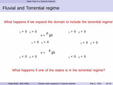
Fluvial and Torrential regime
What happens if we expand the domain to include the torrential regime?
0 5 10 15
h
-25
-20
-15
-10
-5
0
5
10
15
20
25
v
λ1 < 0 λ2 > 0
λ1 > 0 λ2 > 0
λ1 < 0 λ2 < 0
v =√gh
v = −√gh
0 5 10 15
h
-200
-150
-100
-50
0
50
100
150
200
q
λ1 < 0 λ2 > 0
λ1 > 0 λ2 > 0
λ1 < 0 λ2 < 0
What happens if one of the states is in the torrential regime?
Maya Briani (IAC-CNR) Shallow water equations in channel networks May 5 - 2021 25 / 42

Water Flow in a Channel Network
Fluvial and Torrential regime: the case of an incomingcanal
λ1 < 0
λ1 > 0
λ1 < 0
q = h√gh
hφl(h;u0i )
admissible junction values
u0i
Maya Briani (IAC-CNR) Shallow water equations in channel networks May 5 - 2021 26 / 42

Water Flow in a Channel Network
Fluvial and Torrential regime: the case of an incomingcanal
λ1 < 0
λ1 > 0
λ1 < 0
q = h√gh
admissible junction values
u0i
Maya Briani (IAC-CNR) Shallow water equations in channel networks May 5 - 2021 27 / 42

Water Flow in a Channel Network
Fluvial and Torrential regime: outgoing canal
u0j
λ2 > 0
λ2 > 0
λ2 < 0
Figure: |Fr| < 1.Maya Briani (IAC-CNR) Shallow water equations in channel networks May 5 - 2021 28 / 42

Water Flow in a Channel Network
The case study of a simple network
We consider a fictitious network formed by two canals intersecting at onesingle point, which artificially represents the junction.
u01 u02
J
(u∗1, u∗2)
I Conservation of Mass q∗1 = q∗2I Junction Riemann Problem: u∗1 ∈ N (u01), u
∗2 ∈ P(u02)
I we need ? additional conditions
Maya Briani (IAC-CNR) Shallow water equations in channel networks May 5 - 2021 29 / 42

Water Flow in a Channel Network
The case study of a simple network: 1 → 1 Junction
I Conservation of Mass q∗1 = q∗2I Junction Riemann Problem: u∗1 ∈ N (u01), u
∗2 ∈ P(u02)
I we need additional conditions ...
In this simple junction, the natural assumption (consistent with thedynamic of shallow-water equations on a single canal) should be to assumethe conservation of the momentum:
(q∗1)2
h∗1+
1
2g(h∗1)
2 =(q∗2)
2
h∗2+
1
2g(h∗1)
2.
Maya Briani (IAC-CNR) Shallow water equations in channel networks May 5 - 2021 30 / 42

Water Flow in a Channel Network
The case study of a simple network: 1 → 1 Junction
From the conservation of the momentum and q∗1 = q∗2(h2h1
)3
−(2F2
1 + 1)(h2
h1
)+ 2F2
1 = 0
and we have two possible relations for the heights values at the junction:
h∗1 = h∗2 (equal heigths) orh∗2h∗1
=1
2
(−1 +
√1 + 8F2
1
)Let us assume equal water heights, no jump at the junction
h∗1 = h∗2
Then u∗1 = u∗2 = u∗ and the solution is identified (if exists) by theintersection between the two admissible regions N (u01) and P(u02)!
Maya Briani (IAC-CNR) Shallow water equations in channel networks May 5 - 2021 31 / 42

Water Flow in a Channel Network
1 → 1 Junction: Fluvial → Fluvial
ur
ulu∗↙
NB(ul)
PB(ur)
Maya Briani (IAC-CNR) Shallow water equations in channel networks May 5 - 2021 32 / 42

Water Flow in a Channel Network
1 → 1 Junction: Torrential → Fluvial
ur
ul ul
↑u∗
NB(ul)
PA(ur)
Maya Briani (IAC-CNR) Shallow water equations in channel networks May 5 - 2021 33 / 42

Water Flow in a Channel Network
1 → 1 Junction: Torrential → Fluvial
urul
ul ∈ P(ur)
ul
N (ul)
P(ur)
Maya Briani (IAC-CNR) Shallow water equations in channel networks May 5 - 2021 34 / 42

Water Flow in a Channel Network
1 → 1 Junction: Torrential → Torrential
ur
ul
ul /∈ P(ur)ul
N (ul)
P(ur)
No solution!
Maya Briani (IAC-CNR) Shallow water equations in channel networks May 5 - 2021 35 / 42

Water Flow in a Channel Network
The case study of a simple network: 1 → 1 Junction
Assuming h∗1 = h∗2 the solution does not always exist ...
I Assuming h∗1 = h∗2 the solution does not always exist ...
I For h∗1 6= h∗2 we get new possible solutions at the junction ... thecases Torrential→ Fluvial and case Torrential→ Torrential may admitsolution even if their admissible regions have empty intersection in thesubcritical region.
Consistency with the case of a single canal:for appropriate values of (hl, ql), for Torrential→ Fluvial we get the samesolution considering our simple network as a simple canal, i.e. we get astationary shock at the virtual junction called hydraulic jump characterizedindeed by the conservation of the momentum in the transition from asupercritical to subcritical flow.
Maya Briani (IAC-CNR) Shallow water equations in channel networks May 5 - 2021 36 / 42

Water Flow in a Channel Network
Fr > 1 Fr < 1→
Fr > 1 Fr < 1
Figure: Numerical test case for the configuration given in Fig. ??.
Maya Briani (IAC-CNR) Shallow water equations in channel networks May 5 - 2021 37 / 42
Water Flow in a Channel Network
The extension to more complex network is still an Open Problem!
Maya Briani (IAC-CNR) Shallow water equations in channel networks May 5 - 2021 38 / 42

Water Flow in a Channel Network
Conclusion
I Two regimes exist for this hyperbolic system of balance laws: thefluvial, corresponding to eigenvalues with different sign, and thetorrential, corresponding to both positive eigenvalues
I After analyzing the Lax curves for incoming and outgoing canals, weprovide admissibility conditions for Riemann solvers, describingpossible solutions for constant initial data on each canal.
I The simple case of one incoming and outgoing canal is treatedshowing that, already in this simple example, regimes transitionsappear naturally at junctions.
Maya Briani (IAC-CNR) Shallow water equations in channel networks May 5 - 2021 39 / 42

Water Flow in a Channel Network
Further work
I Open canals flow with fluvial to torrential phase transitions on morecomplex networks
I Condition at the node depending on the geometry of the network andcomparison with 2D simulations (joint work with M. Ribot and G.Puppo)
I Problems with non constant bottom level and non constant widthchannels on networks
Maya Briani (IAC-CNR) Shallow water equations in channel networks May 5 - 2021 40 / 42
Water Flow in a Channel Network
Bibliography
M. Briani, G. Puppo, M. Ribot, Angle dependence in couplingconditions for shallow water equations at canal junctions. Preprint2021 hal-03196295. Submitted.
Briani, M.; Piccoli, B. Open canals flow with fluvial to torrential phasetransitions on networks. Networks & Heterogeneous Media, 2018, 13(4) : 663-690.
Briani, M.; Piccoli, B.; Qui, J. M. Notes on RKDG methods forshallow-water equations in canal networks. Journal of ScientificComputing 68(3) (2016).
Maya Briani (IAC-CNR) Shallow water equations in channel networks May 5 - 2021 41 / 42

Thank you very much for your attention
Maya Briani (IAC-CNR) Shallow water equations in channel networks May 5 - 2021 42 / 42

![Deriving one dimensional shallow water equations from mass ...equations over depth Fig.2, a schematic view of hydraulic jump [10]. 2. Derivation of Navier-Stokes equations for shallow](https://img.pdfslide.us/doc/110x75/5e91493e68a8585a8017f546/deriving-one-dimensional-shallow-water-equations-from-mass-equations-over-depth.jpg)