Page 1

SHALE GAS – AN OVERVIEW By Tristan Euzen

IFP Technologies (Canada) Inc.

PREAMBLE

In the fast evolving landscape of unconventional resources, shale gas has been the topic of intense research and

development activities in North America as well as huge investments from independent and major oil & gas

companies over the past few years.

As a North American company focused on franco-canadian technological cooperation, IFP Canada needs to

understand the technological challenges associated with shale gas exploration and development. The aim of this

report is to provide IFP Canada with a comprehensive review of geological as well as “above the ground” factors

that control shale gas prospectivity and productivity. The material used to build this report consists in hundreds of

technical and more general papers, as well as attendance to specialized sessions of oil and gas conferences,

symposiums and short courses. A large part of this material has been compiled in a digital format (pdf) and sorted

by topics and areas (basin or play).

After an introduction presenting the general context of the recent development of the North American shale gas

industry, the first part focuses on the geological factors that control the gas shale prospectivity and productivity.

This chapter discusses the impact, variations and measurement techniques of each of these parameters. The

second part focuses on external factors which relate to our ability to technically and economically extract these

resources. It includes completion and stimulation methods as well as economical, regulatory and environmental

aspects of the shale gas industry.

Page 2

SUMMARY

PREAMBLE 1

SUMMARY 2

LIST OF FIGURES 4

INTRODUCTION 7

DEFINITION OF UNCONVENTIONAL RESOURCES 7

DEFINITION OF GAS SHALE AND SHALE GAS 8

A BRIEF HISTORY OF GAS SHALE DEVELOPMENT 9

GEOLOGICAL CONTROLS ON GAS SHALE PRODUCTIVITY 11

ORGANIC MATTER CONTENT 11

CONTROLS ON ORGANIC MATTER ACCUMULATION 11

VARIABILITY OF TOTAL ORGANIC CARBON (TOC) IN SHALE PLAYS 12

TOC MEASUREMENT AND ESTIMATION TECHNIQUES 15

IMPACT OF TOC ON GAS SHALE PROSPECTIVITY 16

THERMAL MATURITY 17

VARIABILITY OF SOURCE ROCK MATURITY IN SHALE PLAYS 17

IMPACT OF MATURITY ON GAS SHALE PROSPECTIVITY 18

QUANTIFICATION OF SHALE THERMAL MATURITY 19

MINERALOGY 19

CONTROLS ON MINERALOGY IN SHALE 19

VARIABLITY OF THE MINERALOGY OF SHALE PLAYS 19

IMPACT OF MINERALOGY ON GAS SHALE PROSPECTIVITY 21

QUANTIFICATION OF SHALE MINERALOGY 21

PORE SYSTEM 22

CONTROLS ON PORE SYSTEM IN SHALE 22

PORE SYSTEM VARIABILITY IN SHALES 23

QUANTIFICATION OF POROSITY IN SHALE 25

GAS ADSORPTION 26

CONTROLS ON GAS ADSORPTION 27

MEASUREMENT OF ADSORBED GAS 28

IMPACT OF GAS ADSORPTION ON SHALE PROSPECTIVITY 28

PERMEABILITY AND DIFFUSIVITY 29

IMPLICATION FOR FLUID FLOW MODELING AND PERMEABILITY MEASUREMENT 30

Page 3

GEOMECHANICS 32

ROCK MECHANICAL PROPERTIES 32

IN SITU STRESS 35

EXTERNAL CONTROLS ON GAS SHALE PRODUCTIVITY AND DEVELOPMENT 38

WELL AND STIMULATION DESIGN 38

MULTISTAGE HYDRAULIC FRACTURING 38

GEOSTEERING AND COMPLETION DESIGN 39

FRACTURING JOB DESIGN 40

MONITORING AND ASSESMENT OF HYDRAULIC FRACTURING 44

SHALE GAS PRODUCTIVITY AND RESOURCE ASSESSMENT 47

SHALE GAS PRODUCTIVITY 47

SHALE GAS RESOURCES AND PRODUCTION FORECAST 49

SHALE GAS ECONOMICS 52

SHALE GAS BREAKEVEN PRICE 52

SHALE GAS OPERATORS STRATEGIES 53

IMPACT OF FUTURE GAS DEMAND ON SHALE GAS DEVELOPMENT 54

ENVIRONMENTAL IMPACT AND REGULATION OF SHALE GAS DEVELOPMENT 56

SURFACE AND DRINKING WATER CONTAMINATIONS. 56

WATER RESOURCES 59

SURFACE NUISANCES 61

SEISMIC RISKS 63

CONCLUSION: THE ROLE OF SHALE GAS IN THE FUTURE ENERGY MIX 65

REFERENCES 67

Page 4

LIST OF FIGURES

Figure 1: Different types of unconventional plays.

Figure 2: General classification of (a) oil and (b) gas resources based on reservoir and fluid properties.

Figure 3: Increases in production and well count in the Barnett shale from 1990 to 2010.

Figure 4: Estimation of technically recoverable shale gas resources in the world.

Figure 5: Location map of North American shale gas plays.

Figure 6: Controls on organic matter accumulation in sediments.

Figure 7: Time chart of the main North American shale gas plays.

Figure 8: Paleogeographic maps and location of the main organic rich shale basin systems in North America.

Figure 9: Range of TOC of most of the productive and some of the prospective shale gas plays of North America.

Figure 10: a) positive correlation between TOC and micropore volume in Devonian-Mississipian Canadian shales. b)

Relationship between TOC and sorbed gas capacity in Devonian-Mississipian and Jurassic Canadian shales.

Figure 11: Range of maturity (Vitrinite reflectance) of most of the productive and some of the prospective shale

gas plays of North America

Figure 12: Processes leading to the formation of thermogenic gas.

Figure 13: Relative proportion of quartz, clay and carbonate in various shale play in North America.

Figure 14: Influence of mineralogy on shale porosity.

Figure 15: Size of pore throat and particles in sandstones and shale.

Figure 16: Pore types and sizes observed in gas shale reservoirs.

Figure 17: Main types of porosity in shales.

Figure 18: Porosity range of various North American shale plays.

Figure 19: Schematic illustration of gas adsorption.

Figure 20: Langmuir isotherm.

Figure 21: Relation between TOC and methane sorption capacity in Western Canadian shale at 5 MPa and 30⁰C.

Figure 22: Adsorption isotherm of the Barnett shale (composite) at two different temperatures.

Figure 23: Examples of the contribution of adsorbed gas to total gas in place in several shale gas plays.

Figure 24: Comparison of gas flow in micropores where the flow is no-slip and in nanopores where the flow is slip.

Page 5

Figure 25: Different length scale of pore network and gas flow in shale.

Figure 26: Stress and orientation dependency of pulse decay permeability to He measured on core plugs from

various shale plays.

Figure 27: Scale dependency of permeability measured on crushed samples with various particle sizes.

Figure 28: Definition of Poisson’s ratio.

Figure 29: Definition of Young Modulus

Figure 30: Brittleness percentage expressed as a function of Young modulus and Poisson’s ratio.

Figure 30: Triaxial compression apparatus.

Figure 31: Comparison between brittleness calculated from mineralogy and from full wavefrom sonic suite.

Figure 32: Visualization of Young modulus and differential horizontal stress ratio (a measure of stress anisotropy)

derived from 3D seismic of the Colorado shale in Central Alberta.

Figure 33: Complete stress equation implemented into GOHFER software.

Figure 34: Influence of stress regime on stress anisotropy and magnitude.

Figure 34: impact of natural fractures on the propagation of hydraulic fractures in the Barnett shale.

Figure 35: Natural gas chimneys in Marcellus shale.

Figure 36: Illustration of how horizontal multistage fracturing help draining gas from shale matrix.

Figure 37: Average EUR and EUR per frac stage in the Woodford shale.

Figure 38: Horizontal well case study in the Woodford shale.

Figure 39: Eagle Ford well completion example showing the optimization of stage and cluster placement based on

brittleness (RQF) and stress log data.

Figure 40: Relationship between fluid type, reservoir properties and hydraulic fracture geometry.

Figure 41: Average stimulation data for various US shale plays.

Figure 42: Fracturing fluid additives, main compounds and common uses.

Figure 43: McGuire-Sikora folds-of-Increase curves for pseudo-steady flow.

Figure 44: HyWay channel fracturing technology.

Figure 45: Microseismic map and cross-section and pumping chart of a 8 stages hydraulic fracturing in a Barnett

well.

Figure 46: Simulation of the interaction between natural and hydraulic fractures.

Figure 47: Annual gas production from US shale plays during the last decade.

Page 6

Figure 48: Shale versus non-shale U.S. Gas production over time.

Figure 49: Average production curves of core areas of 5 US shale plays (Baihly et al 2010b). Dashed lines are

decline curve analysis forecast.

Figure 50: Fayetteville Shale averaged daily production rate per well in mcf/d as a function of date of first

production.

Figure 51: Different type of resources and their definition.

Figure 52: Example of uncertainty in reserve estimate based on hyperbolic exponent b

Figure 53: Rate transient analysis of a well from the Barnett shale

Figure 54: Breakeven price based on basic economic analysis of core areas of major US shale gas plays.

Figure 55: Comparison of dry gas and liquid rich well economics in Eagle Ford shale.

Figure 56: Eagle Ford leasing movement into oil window

Figure 57: North American shale gas production forecasts

Figure 58: Key stages of hydraulic fracturing water lifecycle and potential contamination risks associated.

Figure 59: Target shale depth and base of treatable groundwater in selected shale plays.

Figure 60: Produced water management by shale gas basin.

Figure 61: Water treatment technologies.

Figure 62: Estimated water needs for drilling and fracturing wells in selected shale gas plays.

Figure 63: Water use by sector in producing area of major shale plays.

Figure 64: Pounds of air pollutants produced per billion of Btu of energy.

Figure 65: EPA natural gas environmental impact assessment and regulation timeline.

Figure 66: Comparison of the magnitude different microseismic events and felt earthquake.

Figure 67: Map showing location of earthquakes, producing Barnett shale gas wells and water disposal wells.

Page 7

INTRODUCTION

As North American conventional hydrocarbon accumulations become increasingly mature, the oil and gas industry

has been recently switching towards unconventional resources, for renewing reserves and securing long term

production and supply. In the recent years, spikes in oil and gas prices and increasing US dependency on foreign oil

and gas import have also put pressure on the industry towards the exploration and development of

unconventional oil and gas resources.

DEFINITION OF UNCONVENTIONAL RESOURCES

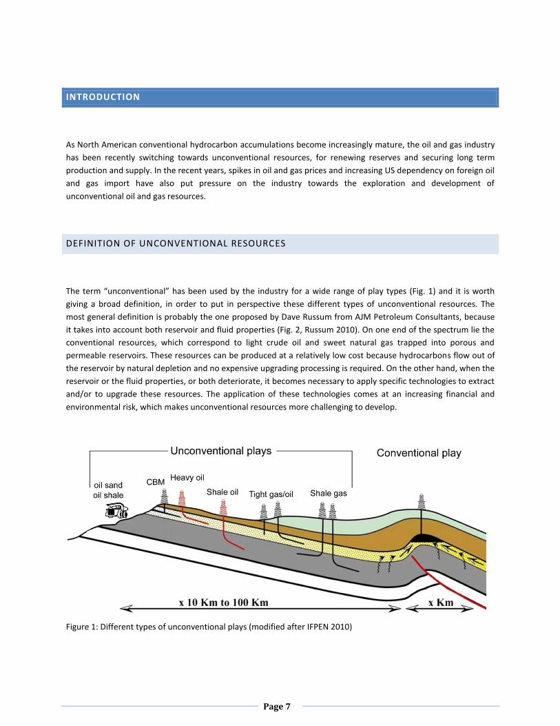
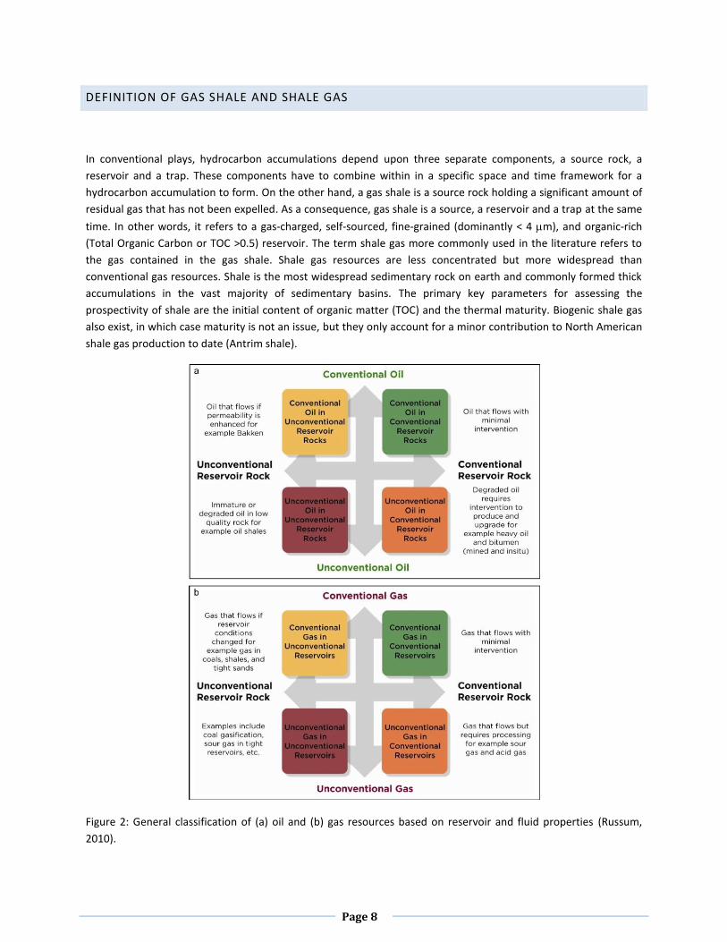
The term “unconventional” has been used by the industry for a wide range of play types (Fig. 1) and it is worth

giving a broad definition, in order to put in perspective these different types of unconventional resources. The

most general definition is probably the one proposed by Dave Russum from AJM Petroleum Consultants, because

it takes into account both reservoir and fluid properties (Fig. 2, Russum 2010). On one end of the spectrum lie the

conventional resources, which correspond to light crude oil and sweet natural gas trapped into porous and

permeable reservoirs. These resources can be produced at a relatively low cost because hydrocarbons flow out of

the reservoir by natural depletion and no expensive upgrading processing is required. On the other hand, when the

reservoir or the fluid properties, or both deteriorate, it becomes necessary to apply specific technologies to extract

and/or to upgrade these resources. The application of these technologies comes at an increasing financial and

environmental risk, which makes unconventional resources more challenging to develop.

Figure 1: Different types of unconventional plays (modified after IFPEN 2010)

Page 8

DEFINITION OF GAS SHALE AND SHALE GAS

In conventional plays, hydrocarbon accumulations depend upon three separate components, a source rock, a

reservoir and a trap. These components have to combine within in a specific space and time framework for a

hydrocarbon accumulation to form. On the other hand, a gas shale is a source rock holding a significant amount of

residual gas that has not been expelled. As a consequence, gas shale is a source, a reservoir and a trap at the same

time. In other words, it refers to a gas-charged, self-sourced, fine-grained (dominantly < 4 m), and organic-rich

(Total Organic Carbon or TOC >0.5) reservoir. The term shale gas more commonly used in the literature refers to

the gas contained in the gas shale. Shale gas resources are less concentrated but more widespread than

conventional gas resources. Shale is the most widespread sedimentary rock on earth and commonly formed thick

accumulations in the vast majority of sedimentary basins. The primary key parameters for assessing the

prospectivity of shale are the initial content of organic matter (TOC) and the thermal maturity. Biogenic shale gas

also exist, in which case maturity is not an issue, but they only account for a minor contribution to North American

shale gas production to date (Antrim shale).

Figure 2: General classification of (a) oil and (b) gas resources based on reservoir and fluid properties (Russum,

2010).

Page 9

A BRIEF HISTORY OF GAS SHALE DEVELOPMENT

Shale gas has been produced as early as 1821, from a natural seepage in fractured Devonian shale in the

Appalachian Mountains (Selley, 2011). Since then, shale gas has been produced throughout the Appalachians,

although produced volumes were marginal. During the 1980’s and 1990’s, a combination of tax incentives,

advances in technologies, operational efficiency, as well as improving understanding of the production

mechanisms, led to the progressive and slow development of several shale plays throughout the United States,

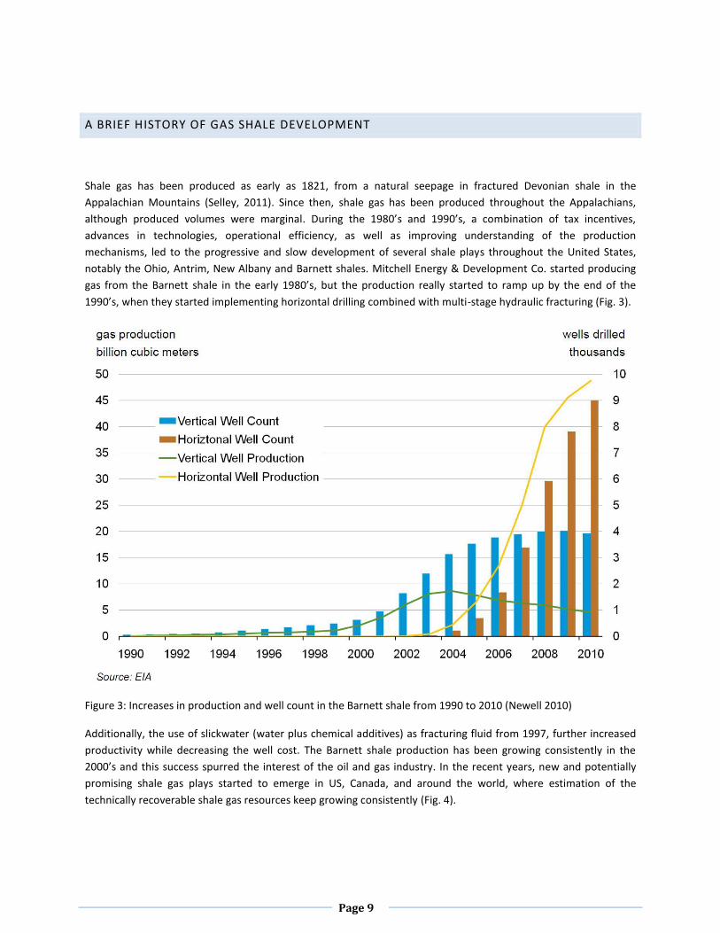
notably the Ohio, Antrim, New Albany and Barnett shales. Mitchell Energy & Development Co. started producing

gas from the Barnett shale in the early 1980’s, but the production really started to ramp up by the end of the

1990’s, when they started implementing horizontal drilling combined with multi-stage hydraulic fracturing (Fig. 3).

Figure 3: Increases in production and well count in the Barnett shale from 1990 to 2010 (Newell 2010)

Additionally, the use of slickwater (water plus chemical additives) as fracturing fluid from 1997, further increased

productivity while decreasing the well cost. The Barnett shale production has been growing consistently in the

2000’s and this success spurred the interest of the oil and gas industry. In the recent years, new and potentially

promising shale gas plays started to emerge in US, Canada, and around the world, where estimation of the

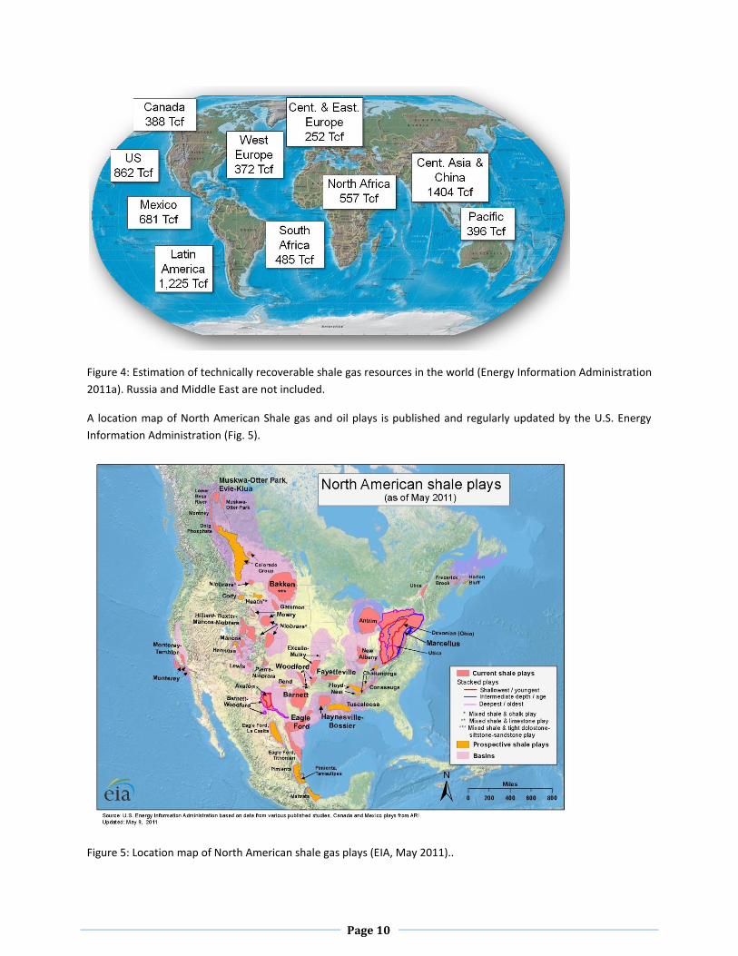
technically recoverable shale gas resources keep growing consistently (Fig. 4).

Page 10

Figure 4: Estimation of technically recoverable shale gas resources in the world (Energy Information Administration

2011a). Russia and Middle East are not included.

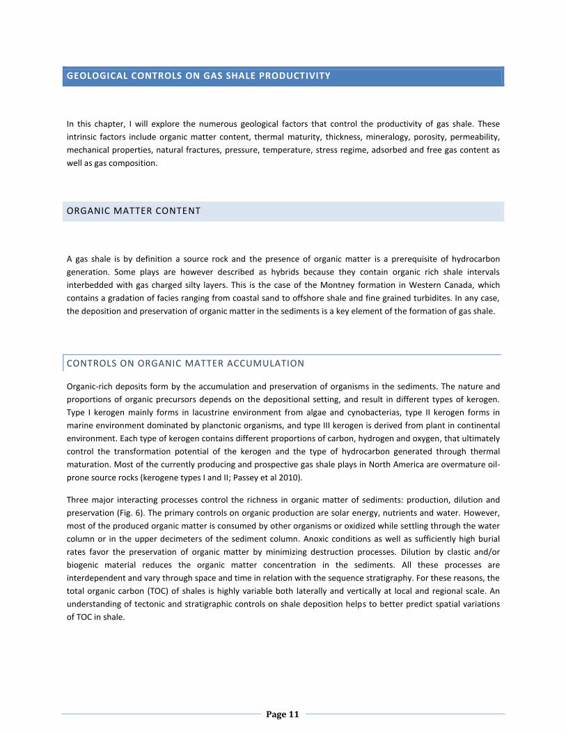
A location map of North American Shale gas and oil plays is published and regularly updated by the U.S. Energy

Information Administration (Fig. 5).

Figure 5: Location map of North American shale gas plays (EIA, May 2011)..

Page 11

GEOLOGICAL CONTROLS ON GAS SHALE PRODUCTIVITY

In this chapter, I will explore the numerous geological factors that control the productivity of gas shale. These

intrinsic factors include organic matter content, thermal maturity, thickness, mineralogy, porosity, permeability,

mechanical properties, natural fractures, pressure, temperature, stress regime, adsorbed and free gas content as

well as gas composition.

ORGANIC MATTER CONTENT

A gas shale is by definition a source rock and the presence of organic matter is a prerequisite of hydrocarbon

generation. Some plays are however described as hybrids because they contain organic rich shale intervals

interbedded with gas charged silty layers. This is the case of the Montney formation in Western Canada, which

contains a gradation of facies ranging from coastal sand to offshore shale and fine grained turbidites. In any case,

the deposition and preservation of organic matter in the sediments is a key element of the formation of gas shale.

CONTROLS ON ORGANIC MATTER ACCUMULATION

Organic-rich deposits form by the accumulation and preservation of organisms in the sediments. The nature and

proportions of organic precursors depends on the depositional setting, and result in different types of kerogen.

Type I kerogen mainly forms in lacustrine environment from algae and cynobacterias, type II kerogen forms in

marine environment dominated by planctonic organisms, and type III kerogen is derived from plant in continental

environment. Each type of kerogen contains different proportions of carbon, hydrogen and oxygen, that ultimately

control the transformation potential of the kerogen and the type of hydrocarbon generated through thermal

maturation. Most of the currently producing and prospective gas shale plays in North America are overmature oil-

prone source rocks (kerogene types I and II; Passey et al 2010).

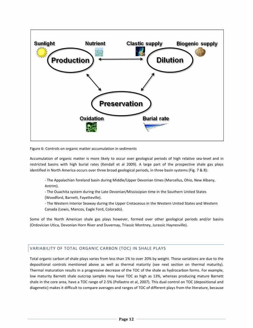
Three major interacting processes control the richness in organic matter of sediments: production, dilution and

preservation (Fig. 6). The primary controls on organic production are solar energy, nutrients and water. However,

most of the produced organic matter is consumed by other organisms or oxidized while settling through the water

column or in the upper decimeters of the sediment column. Anoxic conditions as well as sufficiently high burial

rates favor the preservation of organic matter by minimizing destruction processes. Dilution by clastic and/or

biogenic material reduces the organic matter concentration in the sediments. All these processes are

interdependent and vary through space and time in relation with the sequence stratigraphy. For these reasons, the

total organic carbon (TOC) of shales is highly variable both laterally and vertically at local and regional scale. An

understanding of tectonic and stratigraphic controls on shale deposition helps to better predict spatial variations

of TOC in shale.

Page 12

Figure 6: Controls on organic matter accumulation in sediments

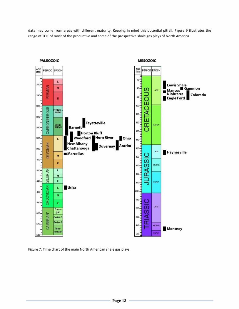
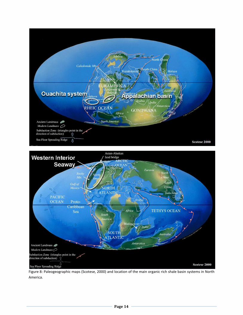
Accumulation of organic matter is more likely to occur over geological periods of high relative sea-level and in

restricted basins with high burial rates (Kendall et al 2009). A large part of the prospective shale gas plays

identified in North America occurs over three broad geological periods, in three basin systems (Fig. 7 & 8):

- The Appalachian foreland basin during Middle/Upper Devonian times (Marcellus, Ohio, New Albany,

Antrim).

- The Ouachita system during the Late Devonian/Mississipian time in the Southern United States

(Woodford, Barnett, Fayetteville).

- The Western Interior Seaway during the Upper Cretaceous in the Western United States and Western

Canada (Lewis, Mancos, Eagle Ford, Colorado).

Some of the North American shale gas plays however, formed over other geological periods and/or basins

(Ordovician Utica, Devonian Horn River and Duvernay, Triassic Montney, Jurassic Haynesville).

VARIABILITY OF TOTAL ORGANIC CARBON (TOC) IN SHALE PLAYS

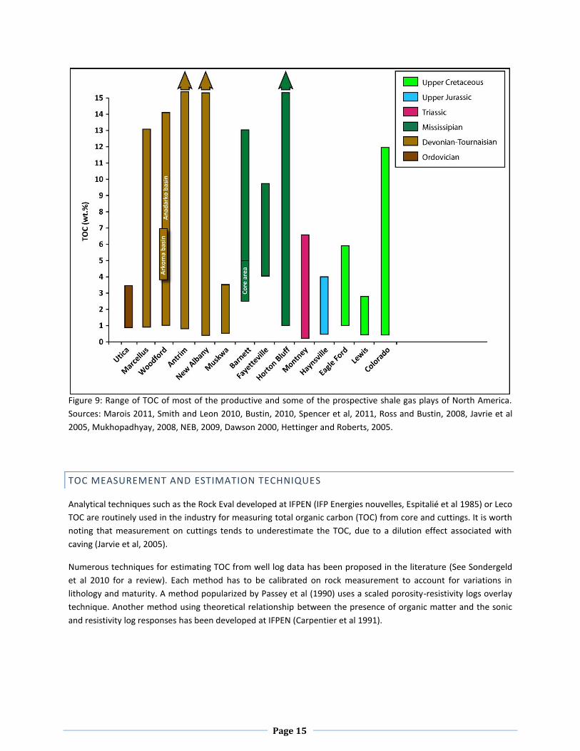
Total organic carbon of shale plays varies from less than 1% to over 20% by weight. These variations are due to the

depositional controls mentioned above as well as thermal maturity (see next section on thermal maturity).

Thermal maturation results in a progressive decrease of the TOC of the shale as hydrocarbon forms. For example,

low maturity Barnett shale outcrop samples may have TOC as high as 13%, whereas producing mature Barnett

shale in the core area, have a TOC range of 2-5% (Pollastro et al, 2007). This dual control on TOC (depositional and

diagenetic) makes it difficult to compare averages and ranges of TOC of different plays from the literature, because

Page 13

data may come from areas with different maturity. Keeping in mind this potential pitfall, Figure 9 illustrates the

range of TOC of most of the productive and some of the prospective shale gas plays of North America.

Figure 7: Time chart of the main North American shale gas plays.

Page 14

Figure 8: Paleogeographic maps (Scotese, 2000) and location of the main organic rich shale basin systems in North

America.

Page 15

Figure 9: Range of TOC of most of the productive and some of the prospective shale gas plays of North America.

Sources: Marois 2011, Smith and Leon 2010, Bustin, 2010, Spencer et al, 2011, Ross and Bustin, 2008, Javrie et al

2005, Mukhopadhyay, 2008, NEB, 2009, Dawson 2000, Hettinger and Roberts, 2005.

TOC MEASUREMENT AND ESTIMATION TECHNIQUES

Analytical techniques such as the Rock Eval developed at IFPEN (IFP Energies nouvelles, Espitalié et al 1985) or Leco

TOC are routinely used in the industry for measuring total organic carbon (TOC) from core and cuttings. It is worth

noting that measurement on cuttings tends to underestimate the TOC, due to a dilution effect associated with

caving (Jarvie et al, 2005).

Numerous techniques for estimating TOC from well log data has been proposed in the literature (See Sondergeld

et al 2010 for a review). Each method has to be calibrated on rock measurement to account for variations in

lithology and maturity. A method popularized by Passey et al (1990) uses a scaled porosity-resistivity logs overlay

technique. Another method using theoretical relationship between the presence of organic matter and the sonic

and resistivity log responses has been developed at IFPEN (Carpentier et al 1991).

Page 16

IMPACT OF TOC ON GAS SHALE PROSPECTIVITY

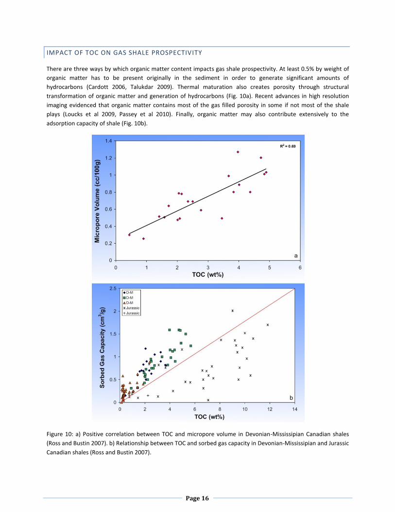
There are three ways by which organic matter content impacts gas shale prospectivity. At least 0.5% by weight of

organic matter has to be present originally in the sediment in order to generate significant amounts of

hydrocarbons (Cardott 2006, Talukdar 2009). Thermal maturation also creates porosity through structural

transformation of organic matter and generation of hydrocarbons (Fig. 10a). Recent advances in high resolution

imaging evidenced that organic matter contains most of the gas filled porosity in some if not most of the shale

plays (Loucks et al 2009, Passey et al 2010). Finally, organic matter may also contribute extensively to the

adsorption capacity of shale (Fig. 10b).

Figure 10: a) Positive correlation between TOC and micropore volume in Devonian-Mississipian Canadian shales

(Ross and Bustin 2007). b) Relationship between TOC and sorbed gas capacity in Devonian-Mississipian and Jurassic

Canadian shales (Ross and Bustin 2007).

Page 17

THERMAL MATURITY

Thermal maturation processes and the type and initial content of organic matter ultimately control the nature,

amount and composition of hydrocarbons generated from organic-rich shales. Consequently, mapping the

variation of maturity within a shale gas play is paramount for defining prospective core areas. Before the recent

gas glut and resulting fall in gas price in North America, companies were chasing overmature shales in the dry gas

window, trying to avoid relative permeability issues due to liquids associated with gas. Since then, the sustained

high oil to gas price differential has driven the industry to focus on the liquid rich part of shale plays and on shale

oil plays because of better economics.

VARIABILITY OF SOURCE ROCK MATURITY IN SHALE PLAYS

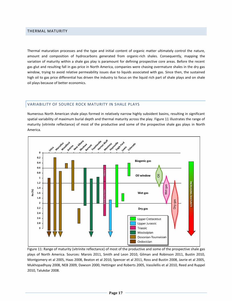
Numerous North American shale plays formed in relatively narrow highly subsident basins, resulting in significant

spatial variability of maximum burial depth and thermal maturity across the play. Figure 11 illustrates the range of

maturity (vitrinite reflectance) of most of the productive and some of the prospective shale gas plays in North

America.

Figure 11: Range of maturity (vitrinite reflectance) of most of the productive and some of the prospective shale gas

plays of North America. Sources: Marois 2011, Smith and Leon 2010, Gilman and Robinson 2011, Bustin 2010,

Montgomery et al 2005, Haas 2008, Beaton et al 2010, Spencer et al 2011, Ross and Bustin 2008, Javrie et al 2005,

Mukhopadhyay 2008, NEB 2009, Dawson 2000, Hettinger and Roberts 2005, Vassilellis et al 2010, Reed and Ruppel

2010, Talukdar 2008.

Page 18

Among the plays shown in Fig. 11, Antrim and Colorado shales are immature and mainly contain biogenic gas,

whereas Haynesville and Muskwa shales are overmature and only contain thermogenic dry gas. In all the other

shale plays, thermal maturity varies widely leading to variable proportion and composition of gas and liquids across

the play.

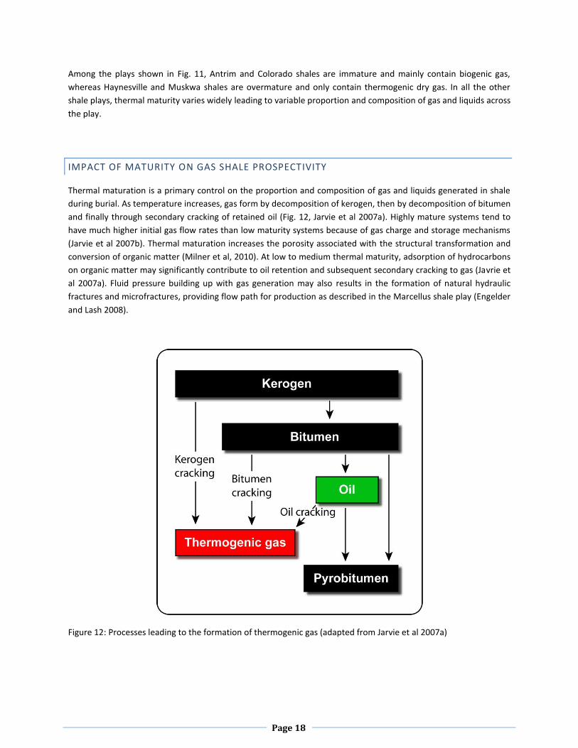
IMPACT OF MATURITY ON GAS SHALE PROSPECTIVITY

Thermal maturation is a primary control on the proportion and composition of gas and liquids generated in shale

during burial. As temperature increases, gas form by decomposition of kerogen, then by decomposition of bitumen

and finally through secondary cracking of retained oil (Fig. 12, Jarvie et al 2007a). Highly mature systems tend to

have much higher initial gas flow rates than low maturity systems because of gas charge and storage mechanisms

(Jarvie et al 2007b). Thermal maturation increases the porosity associated with the structural transformation and

conversion of organic matter (Milner et al, 2010). At low to medium thermal maturity, adsorption of hydrocarbons

on organic matter may significantly contribute to oil retention and subsequent secondary cracking to gas (Javrie et

al 2007a). Fluid pressure building up with gas generation may also results in the formation of natural hydraulic

fractures and microfractures, providing flow path for production as described in the Marcellus shale play (Engelder

and Lash 2008).

Figure 12: Processes leading to the formation of thermogenic gas (adapted from Jarvie et al 2007a)

Page 19

QUANTIFICATION OF SHALE THERMAL MATURITY

The methods for estimating source rock maturity are based on organic matter petrology, experimental pyrolysis

and geochemical analysis.

The vitrinite reflectance method relates on the evolution of optical properties of organic matter with increasing

maturity. Although widely used in the industry, a recent study suggests that this method might underestimate

maturity in some shale plays (Marcellus shale, Laughrey 2008). Other less common petrographic methods include

illite crystallinity, pollen translucency or conodonte transformation index (Laughrey 2008).

In the pyrolysis method, a rock sample is heated and quantities of hydrocarbon expelled are measured (Rock Eval

method developed at IFPEN, Espitalié et al 1985). The temperature of maximum hydrocarbon production (S2)

during the experiment, Tmax, is a measure of the sample maturity.

The biomarkers method relies on the evolution of the composition of organic constituents during thermal

maturation, which can be measured by gas chromatography and mass spectrometry analysis (GC-MS). Another

geochemical approach consists of measuring the stable isotope ratios of gas (Laughrey 2008).

MINERALOGY

Mineralogy is a primary control on the pore network structure of both conventional and unconventional

reservoirs. Furthermore, the initial mineralogical composition of sediments has a strong impact on the nature and

magnitude of diagenetic transformations occurring during their burial history. In gas shales, mineralogy is even

more important because it impacts the mechanical properties of the rocks and how they react to hydraulic

fracturing. Shale refers to sedimentary rocks made up of clay-size particles (< 4 m), but their mineralogy varies

widely within and between shale gas plays. Understanding these variations is necessary to build reliable

petrophysical and geomechanical models and to optimize the placement of fracturing stages.

CONTROLS ON MINERALOGY IN SHALE

The mineralogical composition of shales is controlled by the source of clastics, mechanical and chemical

weathering during erosion, transport and deposition, as well as biogenic production and diagenetic

transformations. These controlling factors vary in time and space, inducing vertical and lateral changes in

mineralogy both at local and regional scales. The analysis of the specific impact of all these controlling factors and

their interactions is beyond the scope of this report.

VARIABLITY OF THE MINERALOGY OF SHALE PLAYS

Most shale lithofacies are a complex mixture of quartz, feldspars, clays, carbonates and accessory minerals (pyrite,

apatite, hematite, anhydrite…). Carbonates as well as silica may be present in the form of fossil fragments like

Page 20

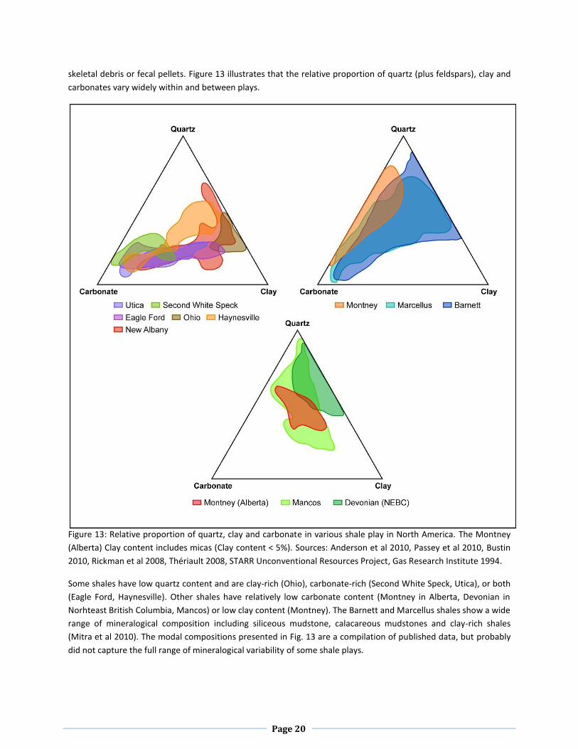
skeletal debris or fecal pellets. Figure 13 illustrates that the relative proportion of quartz (plus feldspars), clay and

carbonates vary widely within and between plays.

Figure 13: Relative proportion of quartz, clay and carbonate in various shale play in North America. The Montney

(Alberta) Clay content includes micas (Clay content < 5%). Sources: Anderson et al 2010, Passey et al 2010, Bustin

2010, Rickman et al 2008, Thériault 2008, STARR Unconventional Resources Project, Gas Research Institute 1994.

Some shales have low quartz content and are clay-rich (Ohio), carbonate-rich (Second White Speck, Utica), or both

(Eagle Ford, Haynesville). Other shales have relatively low carbonate content (Montney in Alberta, Devonian in

Norhteast British Columbia, Mancos) or low clay content (Montney). The Barnett and Marcellus shales show a wide

range of mineralogical composition including siliceous mudstone, calacareous mudstones and clay-rich shales

(Mitra et al 2010). The modal compositions presented in Fig. 13 are a compilation of published data, but probably

did not capture the full range of mineralogical variability of some shale plays.

Page 21

IMPACT OF MINERALOGY ON GAS SHALE PROSPECTIVITY

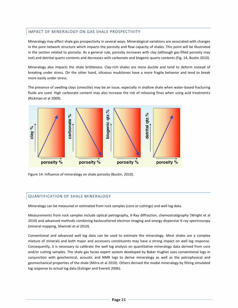
Mineralogy may affect shale gas prospectivity in several ways. Mineralogical variations are associated with changes

in the pore network structure which impacts the porosity and flow capacity of shales. This point will be illustrated

in the section related to porosity. As a general rule, porosity increases with clay (although gas-filled porosity may

not) and detrital quartz contents and decreases with carbonate and biogenic quartz contents (Fig. 14, Bustin 2010).

Mineralogy also impacts the shale brittleness. Clay-rich shales are more ductile and tend to deform instead of

breaking under stress. On the other hand, siliceous mudstones have a more fragile behavior and tend to break

more easily under stress.

The presence of swelling clays (smectite) may be an issue, especially in shallow shale when water-based fracturing

fluids are used. High carbonate content may also increase the risk of releasing fines when using acid treatments

(Rickman et al 2009).

Figure 14: Influence of mineralogy on shale porosity (Bustin, 2010).

QUANTIFICATION OF SHALE MINERALOGY

Mineralogy can be measured or estimated from rock samples (core or cuttings) and well log data.

Measurements from rock samples include optical petrography, X-Ray diffraction, chemostratigraphy (Wright et al

2010) and advanced methods combining backscattered electron imaging and energy dispersive X-ray spectroscopy

(mineral mapping, Sliwinski et al 2010).

Conventional and advanced well log data can be used to estimate the mineralogy. Most shales are a complex

mixture of minerals and both major and accessory constituents may have a strong impact on well log response.

Consequently, it is necessary to calibrate the well log analysis on quantitative mineralogy data derived from core

and/or cutting samples. The shale gas facies expert system developed by Baker Hughes uses conventional logs in

conjunction with geochemical, acoustic and NMR logs to derive mineralogy as well as the petrophysical and

geomechanical properties of the shale (Mitra et al 2010). Others derived the modal mineralogy by fitting simulated

log response to actual log data (Eslinger and Everett 2006).

Page 22

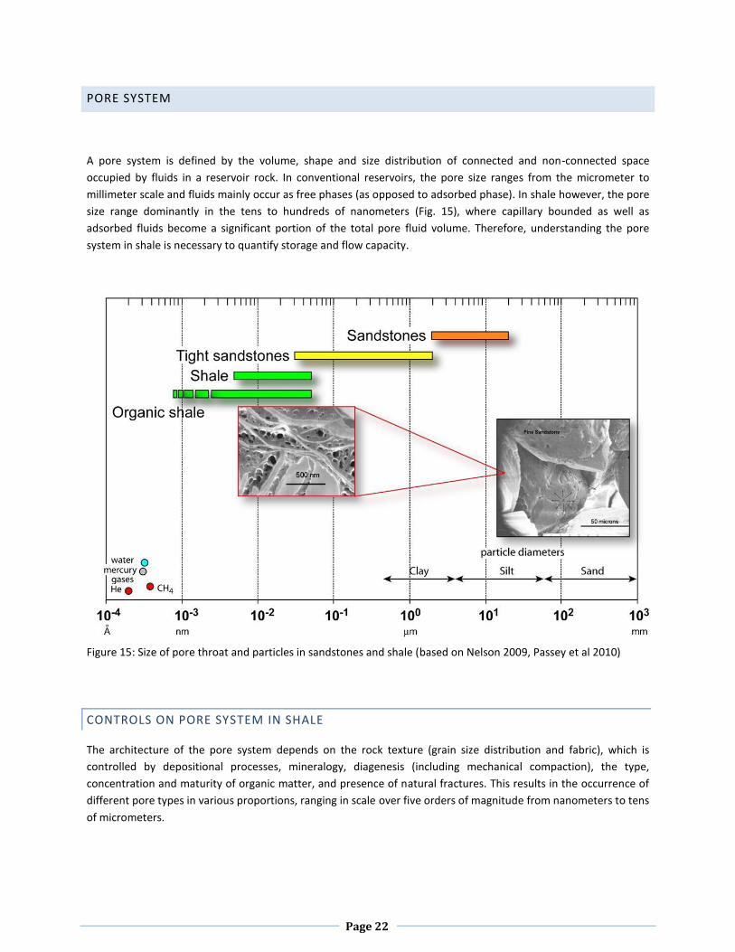
PORE SYSTEM

A pore system is defined by the volume, shape and size distribution of connected and non-connected space

occupied by fluids in a reservoir rock. In conventional reservoirs, the pore size ranges from the micrometer to

millimeter scale and fluids mainly occur as free phases (as opposed to adsorbed phase). In shale however, the pore

size range dominantly in the tens to hundreds of nanometers (Fig. 15), where capillary bounded as well as

adsorbed fluids become a significant portion of the total pore fluid volume. Therefore, understanding the pore

system in shale is necessary to quantify storage and flow capacity.

Figure 15: Size of pore throat and particles in sandstones and shale (based on Nelson 2009, Passey et al 2010)

CONTROLS ON PORE SYSTEM IN SHALE

The architecture of the pore system depends on the rock texture (grain size distribution and fabric), which is

controlled by depositional processes, mineralogy, diagenesis (including mechanical compaction), the type,

concentration and maturity of organic matter, and presence of natural fractures. This results in the occurrence of

different pore types in various proportions, ranging in scale over five orders of magnitude from nanometers to tens

of micrometers.

Page 23

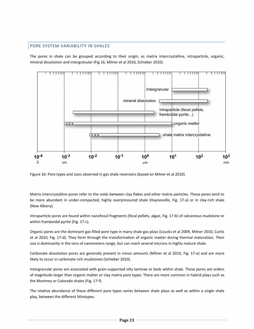
PORE SYSTEM VARIABIL ITY IN SHALES

The pores in shale can be grouped according to their origin, as matrix intercrystalline, intraparticle, organic,

mineral dissolution and intergranular (Fig 16, Milner et al 2010, Schieber 2010).

Figure 16: Pore types and sizes observed in gas shale reservoirs (based on Milner et al 2010)

Matrix intercrystalline pores refer to the voids between clay flakes and other matrix particles. These pores tend to

be more abundant in under-compacted, highly overpressured shale (Haynesville, Fig. 17-a) or in clay-rich shale

(New Albany).

Intraparticle pores are found within nanofossil fragments (fecal pellets, algae, Fig. 17-b) of calcareous mudstone or

within framboidal pyrite (Fig. 17-c).

Organic pores are the dominant gas-filled pore type in many shale gas plays (Loucks et al 2009, Milner 2010, Curtis

et al 2010, Fig. 17-d). They form through the transformation of organic matter during thermal maturation. Their

size is dominantly in the tens of nanometers range, but can reach several microns in highly mature shale.

Carbonate dissolution pores are generally present in minor amounts (Milner et al 2010, Fig. 17-e) and are more

likely to occur in carbonate rich mudstones (Schieber 2010).

Intergranular pores are associated with grain-supported silty laminae or beds within shale. These pores are orders

of magnitude larger than organic matter or clay matrix pore types. There are more common in hybrid plays such as

the Montney or Colorado shales (Fig. 17-f).

The relative abundance of these different pore types varies between shale plays as well as within a single shale

play, between the different lithotypes.

Page 24

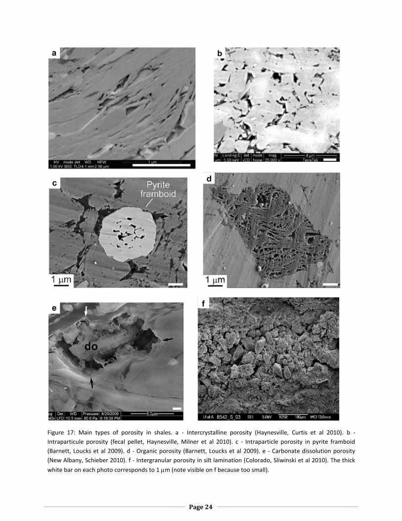
Figure 17: Main types of porosity in shales. a - Intercrystalline porosity (Haynesville, Curtis et al 2010). b -

Intraparticule porosity (fecal pellet, Haynesville, Milner et al 2010). c - Intraparticle porosity in pyrite framboid

(Barnett, Loucks et al 2009). d - Organic porosity (Barnett, Loucks et al 2009). e - Carbonate dissolution porosity

(New Albany, Schieber 2010). f - Intergranular porosity in silt lamination (Colorado, Sliwinski et al 2010). The thick

white bar on each photo corresponds to 1 m (note visible on f because too small).

Page 25

QUANTIFICATION OF POROSITY IN SHALE

Estimation of porosity and more specifically of gas-filled porosity is necessary to quantify original gas in place

(OGIP) in shale. Due to the very small pore size, the result of porosity measurement is very sensitive to the

experimental method used and has been shown to vary significantly, even between different labs using the same

method (Sondergeld et al 2010, Passey et al 2010). This is an important point because small variations of porosity

value have a greater impact on OGIP estimates in low porosity rocks.

Helium pycnometry on core plug tends underestimates porosity because of abundant non-connected micropores.

For this reason, a method using crushed samples is most commonly used in shale (Luffel and Guirdy 1992).

Mercury porosimetry on preserved (no fluid extraction) crushed sample has also been proposed as a good

approximation for gas filled porosity (Olson and Grigg 2008). Several authors advocate the use of standardized lab

protocols specific to shale reservoirs, in order to minimize inconsistencies between labs (Bustin et al 2008a,

Sondergeld et al 2010, Passey et al 2010).

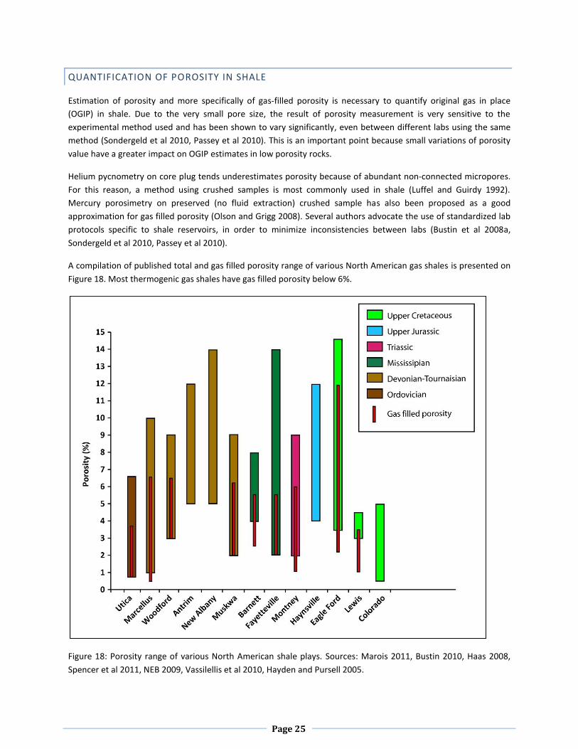
A compilation of published total and gas filled porosity range of various North American gas shales is presented on

Figure 18. Most thermogenic gas shales have gas filled porosity below 6%.

Figure 18: Porosity range of various North American shale plays. Sources: Marois 2011, Bustin 2010, Haas 2008,

Spencer et al 2011, NEB 2009, Vassilellis et al 2010, Hayden and Pursell 2005.

Page 26

The presence of clay, organic matter as well as heavy minerals makes it challenging to derive shale porosity from

conventional log analysis. To overcome this difficulty, it is necessary to calibrate conventional as well as advanced

logging tool using mineralogical data derived from core or cuttings (Mitra et al 2010).

GAS ADSORPTION

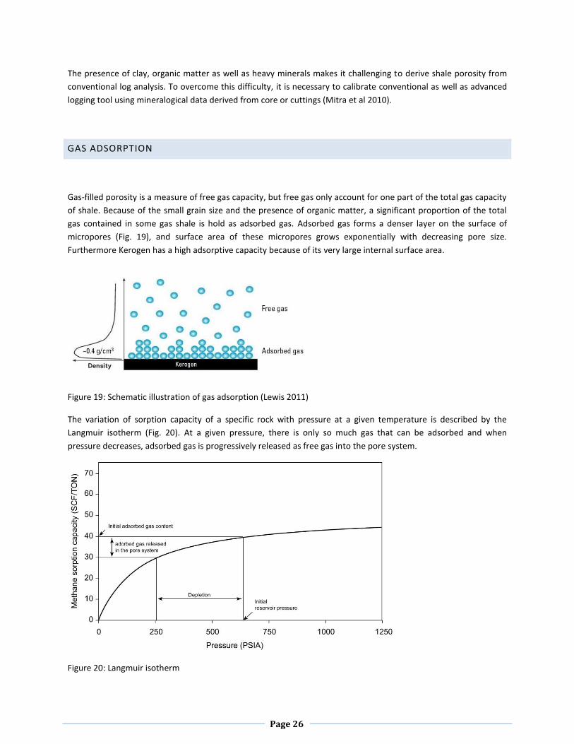
Gas-filled porosity is a measure of free gas capacity, but free gas only account for one part of the total gas capacity

of shale. Because of the small grain size and the presence of organic matter, a significant proportion of the total

gas contained in some gas shale is hold as adsorbed gas. Adsorbed gas forms a denser layer on the surface of

micropores (Fig. 19), and surface area of these micropores grows exponentially with decreasing pore size.

Furthermore Kerogen has a high adsorptive capacity because of its very large internal surface area.

Figure 19: Schematic illustration of gas adsorption (Lewis 2011)

The variation of sorption capacity of a specific rock with pressure at a given temperature is described by the

Langmuir isotherm (Fig. 20). At a given pressure, there is only so much gas that can be adsorbed and when

pressure decreases, adsorbed gas is progressively released as free gas into the pore system.

Figure 20: Langmuir isotherm

Page 27

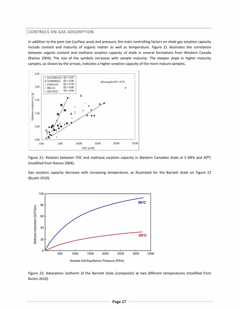
CONTROLS ON GAS ADSORPTION

In addition to the pore size (surface area) and pressure, the main controlling factors on shale gas sorption capacity

include content and maturity of organic matter as well as temperature. Figure 21 illustrates the correlation

between organic content and methane sorption capacity of shale in several formations from Western Canada

(Ramos 2004). The size of the symbols increases with sample maturity. The steeper slope in higher maturity

samples, as shown by the arrows, indicates a higher sorption capacity of the more mature samples.

Figure 21: Relation between TOC and methane sorption capacity in Western Canadian shale at 5 MPa and 30⁰C

(modified from Ramos 2004).

Gas sorption capacity decrease with increasing temperature, as illustrated for the Barnett shale on Figure 22

(Bustin 2010).

Figure 22: Adsorption isotherm of the Barnett shale (composite) at two different temperatures (modified from

Bustin 2010)

Page 28

MEASUREMENT OF ADSORBED GAS

The sorption capacity of shale can be measured either by desorption isotherm or by equilibrium adsorption

isotherm and is expressed in standard cubic feet per ton of rock (SCF/ton). The desorption isotherm method,

commonly used for CBM, consists in placing a core sample inside a sealed canister at the well site and measuring

the volumes of gas evolved with decreasing pressure at reservoir temperature (Waechter et al 2004). Bustin et al

(2008) suggest that the gas released from canister desorption of shale gas contains not only desorbed gas, but also

free gas retained in the core due to the very low permeability of shale. Equilibrium adsorption isotherm method

overcomes this difficulty, by measuring the gas sorption capacity to methane with increasing pressure of a

previously desorbed sample (Bustin et al 2008a). This method requires an accurate estimate of the moisture

content, temperature and pressure of the reservoir, in order to accurately measure in situ sorption capacity.

IMPACT OF GAS ADSORPTION ON SHALE PROSPECTIVITY

The knowledge of gas sorption capacity is essential for estimating the gas in place as well as for predicting the flow

characteristics of shale gas.

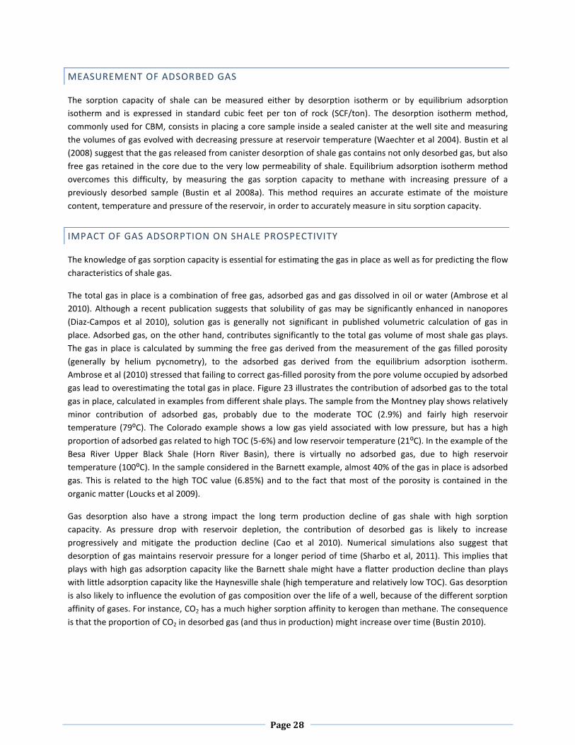
The total gas in place is a combination of free gas, adsorbed gas and gas dissolved in oil or water (Ambrose et al

2010). Although a recent publication suggests that solubility of gas may be significantly enhanced in nanopores

(Diaz-Campos et al 2010), solution gas is generally not significant in published volumetric calculation of gas in

place. Adsorbed gas, on the other hand, contributes significantly to the total gas volume of most shale gas plays.

The gas in place is calculated by summing the free gas derived from the measurement of the gas filled porosity

(generally by helium pycnometry), to the adsorbed gas derived from the equilibrium adsorption isotherm.

Ambrose et al (2010) stressed that failing to correct gas-filled porosity from the pore volume occupied by adsorbed

gas lead to overestimating the total gas in place. Figure 23 illustrates the contribution of adsorbed gas to the total

gas in place, calculated in examples from different shale plays. The sample from the Montney play shows relatively

minor contribution of adsorbed gas, probably due to the moderate TOC (2.9%) and fairly high reservoir

temperature (79⁰C). The Colorado example shows a low gas yield associated with low pressure, but has a high

proportion of adsorbed gas related to high TOC (5-6%) and low reservoir temperature (21⁰C). In the example of the

Besa River Upper Black Shale (Horn River Basin), there is virtually no adsorbed gas, due to high reservoir

temperature (100⁰C). In the sample considered in the Barnett example, almost 40% of the gas in place is adsorbed

gas. This is related to the high TOC value (6.85%) and to the fact that most of the porosity is contained in the

organic matter (Loucks et al 2009).

Gas desorption also have a strong impact the long term production decline of gas shale with high sorption

capacity. As pressure drop with reservoir depletion, the contribution of desorbed gas is likely to increase

progressively and mitigate the production decline (Cao et al 2010). Numerical simulations also suggest that

desorption of gas maintains reservoir pressure for a longer period of time (Sharbo et al, 2011). This implies that

plays with high gas adsorption capacity like the Barnett shale might have a flatter production decline than plays

with little adsorption capacity like the Haynesville shale (high temperature and relatively low TOC). Gas desorption

is also likely to influence the evolution of gas composition over the life of a well, because of the different sorption

affinity of gases. For instance, CO2 has a much higher sorption affinity to kerogen than methane. The consequence

is that the proportion of CO2 in desorbed gas (and thus in production) might increase over time (Bustin 2010).

Page 29

Figure 23: Examples of the contribution of adsorbed gas to total gas in place in several shale gas plays (note the

different unit used for GIP between top and bottom diagrams). Source: Bustin 2010, Ross and Bustin 2008 and

Jarvie et al 2005.

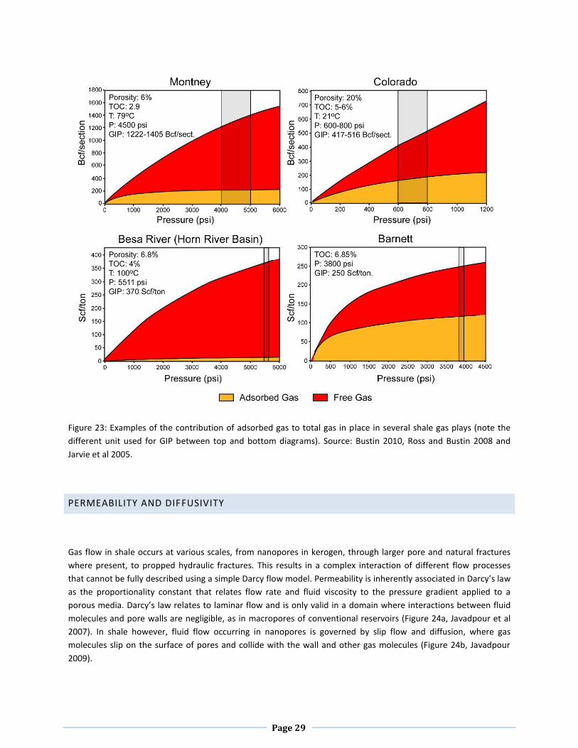
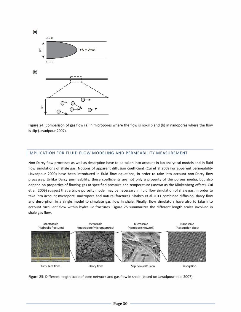
PERMEABILITY AND DIFFUSIVITY

Gas flow in shale occurs at various scales, from nanopores in kerogen, through larger pore and natural fractures

where present, to propped hydraulic fractures. This results in a complex interaction of different flow processes

that cannot be fully described using a simple Darcy flow model. Permeability is inherently associated in Darcy’s law

as the proportionality constant that relates flow rate and fluid viscosity to the pressure gradient applied to a

porous media. Darcy’s law relates to laminar flow and is only valid in a domain where interactions between fluid

molecules and pore walls are negligible, as in macropores of conventional reservoirs (Figure 24a, Javadpour et al

2007). In shale however, fluid flow occurring in nanopores is governed by slip flow and diffusion, where gas

molecules slip on the surface of pores and collide with the wall and other gas molecules (Figure 24b, Javadpour

2009).

Page 30

Figure 24: Comparison of gas flow (a) in micropores where the flow is no-slip and (b) in nanopores where the flow

is slip (Javadpour 2007).

IMPLICATION FOR FLUID FLOW MODELING AND PERMEABILITY MEASUREMENT

Non-Darcy flow processes as well as desorption have to be taken into account in lab analytical models and in fluid

flow simulations of shale gas. Notions of apparent diffusion coefficient (Cui et al 2009) or apparent permeability

(Javadpour 2009) have been introduced in fluid flow equations, in order to take into account non-Darcy flow

processes. Unlike Darcy permeability, these coefficients are not only a property of the porous media, but also

depend on properties of flowing gas at specified pressure and temperature (known as the Klinkenberg effect). Cui

et al (2009) suggest that a triple porosity model may be necessary in fluid flow simulation of shale gas, in order to

take into account micropore, macropore and natural fractures. Shabro et al 2011 combined diffusion, darcy flow

and desorption in a single model to simulate gas flow in shale. Finally, flow simulators have also to take into

account turbulent flow within hydraulic fractures. Figure 25 summarizes the different length scales involved in

shale gas flow.

Figure 25: Different length scale of pore network and gas flow in shale (based on Javadpour et al 2007).

Page 31

Considering the variety of processes and scales involved in the flow of gas in shale, it is important to understand

(1) the scale dependency of permeability measurement and (2) the significance of a measured permeability value

in relation to non-darcy flow processes.

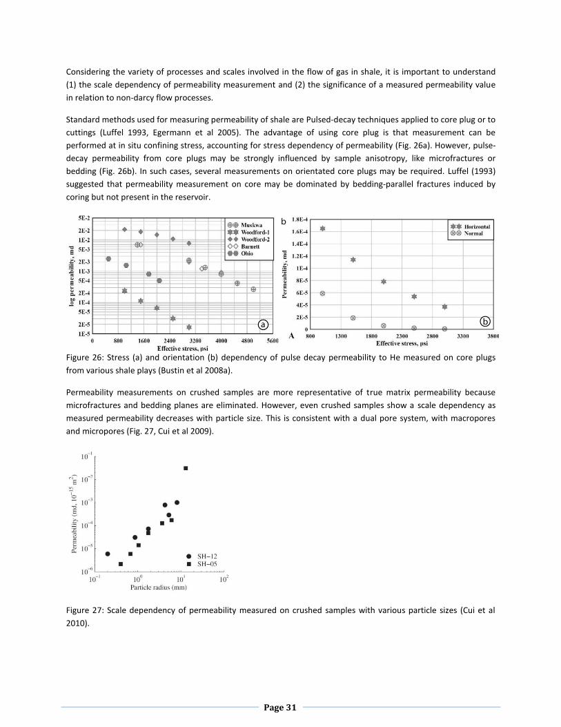
Standard methods used for measuring permeability of shale are Pulsed-decay techniques applied to core plug or to

cuttings (Luffel 1993, Egermann et al 2005). The advantage of using core plug is that measurement can be

performed at in situ confining stress, accounting for stress dependency of permeability (Fig. 26a). However, pulse-

decay permeability from core plugs may be strongly influenced by sample anisotropy, like microfractures or

bedding (Fig. 26b). In such cases, several measurements on orientated core plugs may be required. Luffel (1993)

suggested that permeability measurement on core may be dominated by bedding-parallel fractures induced by

coring but not present in the reservoir.

Figure 26: Stress (a) and orientation (b) dependency of pulse decay permeability to He measured on core plugs

from various shale plays (Bustin et al 2008a).

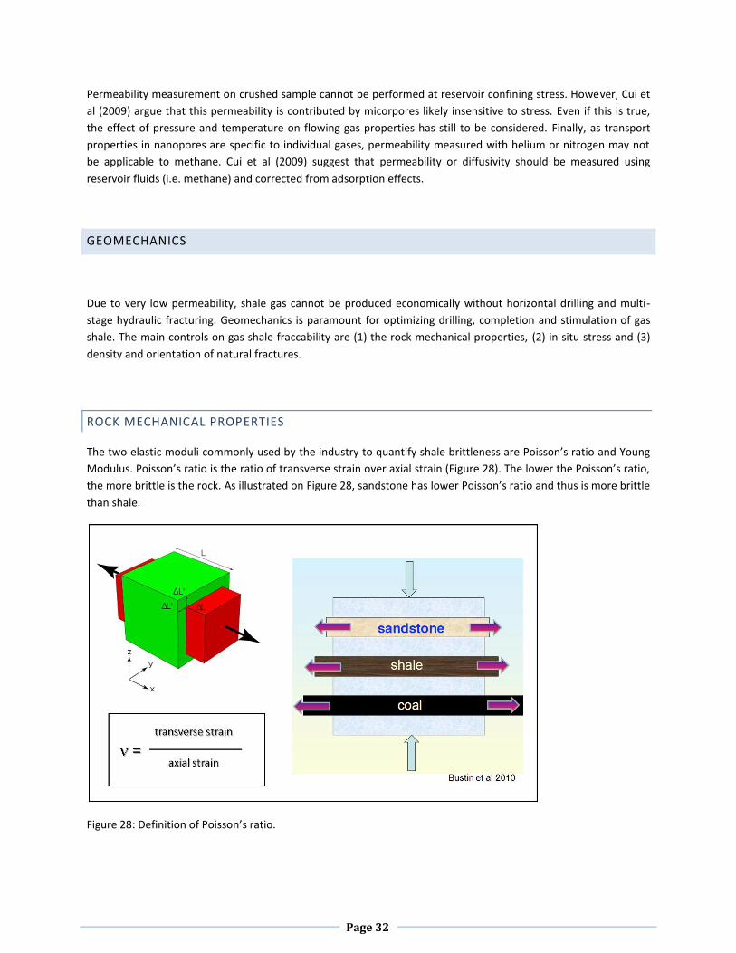
Permeability measurements on crushed samples are more representative of true matrix permeability because

microfractures and bedding planes are eliminated. However, even crushed samples show a scale dependency as

measured permeability decreases with particle size. This is consistent with a dual pore system, with macropores

and micropores (Fig. 27, Cui et al 2009).

Figure 27: Scale dependency of permeability measured on crushed samples with various particle sizes (Cui et al

2010).

Page 32

Permeability measurement on crushed sample cannot be performed at reservoir confining stress. However, Cui et

al (2009) argue that this permeability is contributed by micorpores likely insensitive to stress. Even if this is true,

the effect of pressure and temperature on flowing gas properties has still to be considered. Finally, as transport

properties in nanopores are specific to individual gases, permeability measured with helium or nitrogen may not

be applicable to methane. Cui et al (2009) suggest that permeability or diffusivity should be measured using

reservoir fluids (i.e. methane) and corrected from adsorption effects.

GEOMECHANICS

Due to very low permeability, shale gas cannot be produced economically without horizontal drilling and multi-

stage hydraulic fracturing. Geomechanics is paramount for optimizing drilling, completion and stimulation of gas

shale. The main controls on gas shale fraccability are (1) the rock mechanical properties, (2) in situ stress and (3)

density and orientation of natural fractures.

ROCK MECHANICAL PROPERTIES

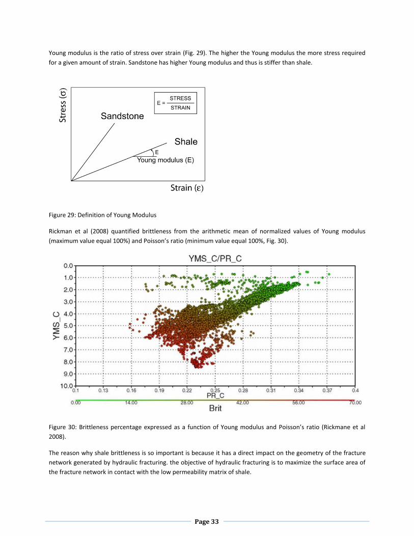
The two elastic moduli commonly used by the industry to quantify shale brittleness are Poisson’s ratio and Young

Modulus. Poisson’s ratio is the ratio of transverse strain over axial strain (Figure 28). The lower the Poisson’s ratio,

the more brittle is the rock. As illustrated on Figure 28, sandstone has lower Poisson’s ratio and thus is more brittle

than shale.

Figure 28: Definition of Poisson’s ratio.

Page 33

Young modulus is the ratio of stress over strain (Fig. 29). The higher the Young modulus the more stress required

for a given amount of strain. Sandstone has higher Young modulus and thus is stiffer than shale.

Figure 29: Definition of Young Modulus

Rickman et al (2008) quantified brittleness from the arithmetic mean of normalized values of Young modulus

(maximum value equal 100%) and Poisson’s ratio (minimum value equal 100%, Fig. 30).

Figure 30: Brittleness percentage expressed as a function of Young modulus and Poisson’s ratio (Rickmane et al

2008).

The reason why shale brittleness is so important is because it has a direct impact on the geometry of the fracture

network generated by hydraulic fracturing. the objective of hydraulic fracturing is to maximize the surface area of

the fracture network in contact with the low permeability matrix of shale.

Page 34

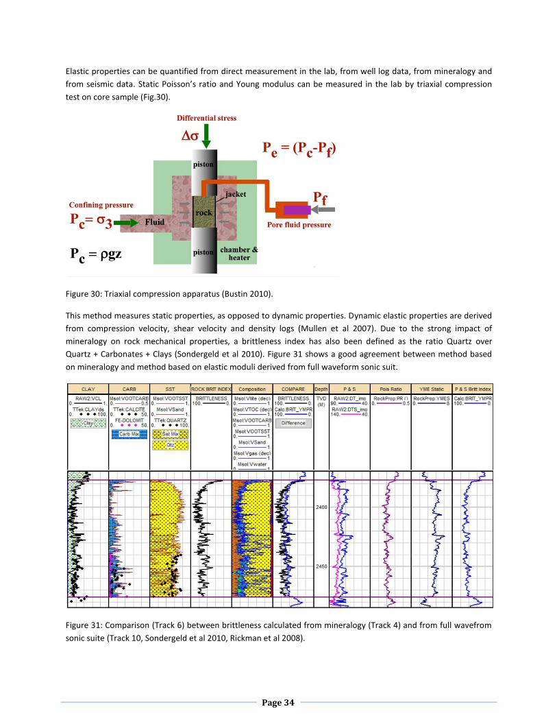
Elastic properties can be quantified from direct measurement in the lab, from well log data, from mineralogy and

from seismic data. Static Poisson’s ratio and Young modulus can be measured in the lab by triaxial compression

test on core sample (Fig.30).

Figure 30: Triaxial compression apparatus (Bustin 2010).

This method measures static properties, as opposed to dynamic properties. Dynamic elastic properties are derived

from compression velocity, shear velocity and density logs (Mullen et al 2007). Due to the strong impact of

mineralogy on rock mechanical properties, a brittleness index has also been defined as the ratio Quartz over

Quartz + Carbonates + Clays (Sondergeld et al 2010). Figure 31 shows a good agreement between method based

on mineralogy and method based on elastic moduli derived from full waveform sonic suit.

Figure 31: Comparison (Track 6) between brittleness calculated from mineralogy (Track 4) and from full wavefrom

sonic suite (Track 10, Sondergeld et al 2010, Rickman et al 2008).

Page 35

In the absence of dipole sonic logs (providing shear velocity), Mullen et al (2007) proposed a composite rock

property model (CRPM) in which they derived rock mechanical properties from conventional logs using multiple

petrophysical relationships and neural network methods.

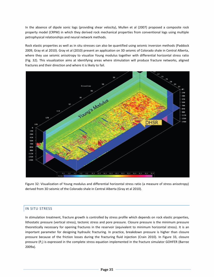
Rock elastic properties as well as in situ stresses can also be quantified using seismic inversion methods (Paddock

2009, Gray et al 2010). Gray et al (2010) present an application on 3D seismic of Colorado shale in Central Alberta,

where they use seismic anisotropy to visualize Young modulus together with differential horizontal stress ratio

(Fig. 32). This visualization aims at identifying areas where stimulation will produce fracture networks, aligned

fractures and their direction and where it is likely to fail.

Figure 32: Visualization of Young modulus and differential horizontal stress ratio (a measure of stress anisotropy)

derived from 3D seismic of the Colorado shale in Central Alberta (Gray et al 2010).

IN SITU STRESS

In stimulation treatment, fracture growth is controlled by stress profile which depends on rock elastic properties,

lithostatic pressure (vertical stress), tectonic stress and pore pressure. Closure pressure is the minimum pressure

theoretically necessary for opening fractures in the reservoir (equivalent to minimum horizontal stress). It is an

important parameter for designing hydraulic fracturing. In practice, breakdown pressure is higher than closure

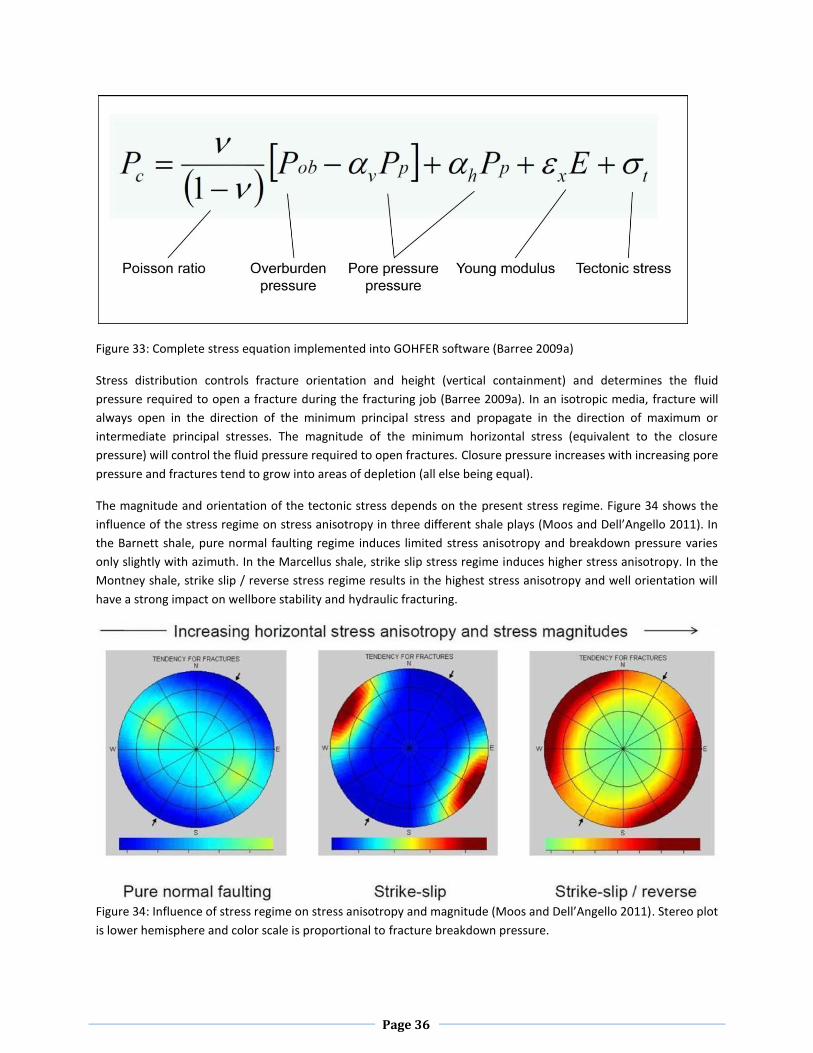
pressure because of the friction losses during the fracturing fluid injection (Crain 2010). In Figure 33, closure

pressure (Pc) is expressed in the complete stress equation implemented in the fracture simulator GOHFER (Barree

2009a).

Page 36

Figure 33: Complete stress equation implemented into GOHFER software (Barree 2009a)

Stress distribution controls fracture orientation and height (vertical containment) and determines the fluid

pressure required to open a fracture during the fracturing job (Barree 2009a). In an isotropic media, fracture will

always open in the direction of the minimum principal stress and propagate in the direction of maximum or

intermediate principal stresses. The magnitude of the minimum horizontal stress (equivalent to the closure

pressure) will control the fluid pressure required to open fractures. Closure pressure increases with increasing pore

pressure and fractures tend to grow into areas of depletion (all else being equal).

The magnitude and orientation of the tectonic stress depends on the present stress regime. Figure 34 shows the

influence of the stress regime on stress anisotropy in three different shale plays (Moos and Dell’Angello 2011). In

the Barnett shale, pure normal faulting regime induces limited stress anisotropy and breakdown pressure varies

only slightly with azimuth. In the Marcellus shale, strike slip stress regime induces higher stress anisotropy. In the

Montney shale, strike slip / reverse stress regime results in the highest stress anisotropy and well orientation will

have a strong impact on wellbore stability and hydraulic fracturing.

Figure 34: Influence of stress regime on stress anisotropy and magnitude (Moos and Dell’Angello 2011). Stereo plot

is lower hemisphere and color scale is proportional to fracture breakdown pressure.

Page 37

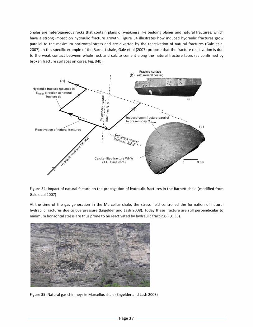
Shales are heterogeneous rocks that contain plans of weakness like bedding planes and natural fractures, which

have a strong impact on hydraulic fracture growth. Figure 34 illustrates how induced hydraulic fractures grow

parallel to the maximum horizontal stress and are diverted by the reactivation of natural fractures (Gale et al

2007). In this specific example of the Barnett shale, Gale et al (2007) propose that the fracture reactivation is due

to the weak contact between whole rock and calcite cement along the natural fracture faces (as confirmed by

broken fracture surfaces on cores, Fig. 34b).

Figure 34: impact of natural facture on the propagation of hydraulic fractures in the Barnett shale (modified from

Gale et al 2007)

At the time of the gas generation in the Marcellus shale, the stress field controlled the formation of natural

hydraulic fractures due to overpressure (Engelder and Lash 2008). Today these fracture are still perpendicular to

minimum horizontal stress are thus prone to be reactivated by hydraulic fraccing (Fig. 35).

Figure 35: Natural gas chimneys in Marcellus shale (Engelder and Lash 2008)

Page 38

EXTERNAL CONTROLS ON GAS SHALE PRODUCTIVITY AND DEVELOPMENT

External controls on shale gas productivity relate to technological as well as economical, environmental and

regulatory requirements that make shale gas a viable and sustainable resource. Although the presence of gas in

shale has been known for many years, it didn’t make sense to even estimate these resources until the combination

of horizontal drilling and multistage hydraulic fracturing made it technically recoverable. It is only after two

decades of experimentation and development in the Barnett shale that the shale gas wave started growing with

the emersion of several promising shale play in North America, and now around the world.

WELL AND STIMULATION DESIGN

MULTISTAGE HYDRAULIC FRACTURING

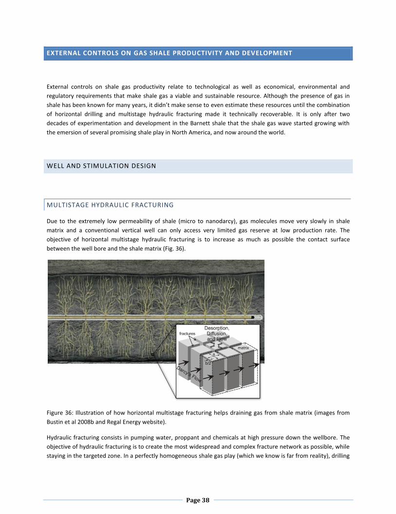
Due to the extremely low permeability of shale (micro to nanodarcy), gas molecules move very slowly in shale

matrix and a conventional vertical well can only access very limited gas reserve at low production rate. The

objective of horizontal multistage hydraulic fracturing is to increase as much as possible the contact surface

between the well bore and the shale matrix (Fig. 36).

Figure 36: Illustration of how horizontal multistage fracturing helps draining gas from shale matrix (images from

Bustin et al 2008b and Regal Energy website).

Hydraulic fracturing consists in pumping water, proppant and chemicals at high pressure down the wellbore. The

objective of hydraulic fracturing is to create the most widespread and complex fracture network as possible, while

staying in the targeted zone. In a perfectly homogeneous shale gas play (which we know is far from reality), drilling

Page 39

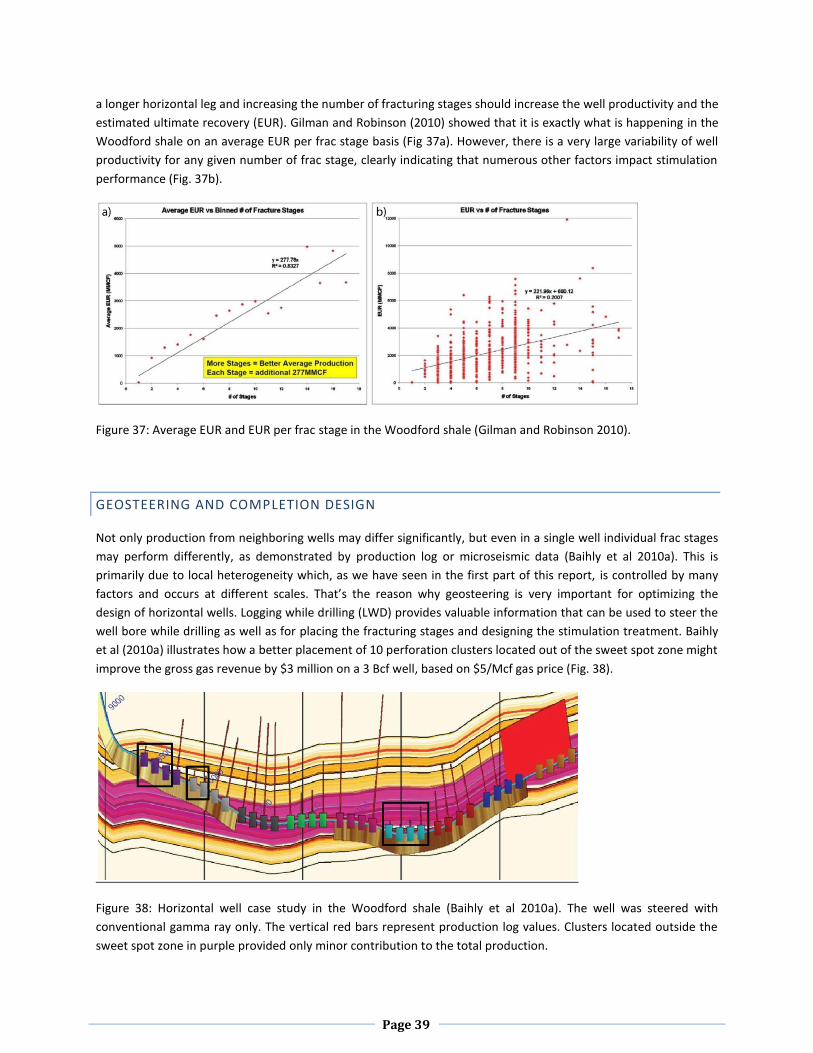
a longer horizontal leg and increasing the number of fracturing stages should increase the well productivity and the

estimated ultimate recovery (EUR). Gilman and Robinson (2010) showed that it is exactly what is happening in the

Woodford shale on an average EUR per frac stage basis (Fig 37a). However, there is a very large variability of well

productivity for any given number of frac stage, clearly indicating that numerous other factors impact stimulation

performance (Fig. 37b).

Figure 37: Average EUR and EUR per frac stage in the Woodford shale (Gilman and Robinson 2010).

GEOSTEERING AND COMPLETION DESIGN

Not only production from neighboring wells may differ significantly, but even in a single well individual frac stages

may perform differently, as demonstrated by production log or microseismic data (Baihly et al 2010a). This is

primarily due to local heterogeneity which, as we have seen in the first part of this report, is controlled by many

factors and occurs at different scales. That’s the reason why geosteering is very important for optimizing the

design of horizontal wells. Logging while drilling (LWD) provides valuable information that can be used to steer the

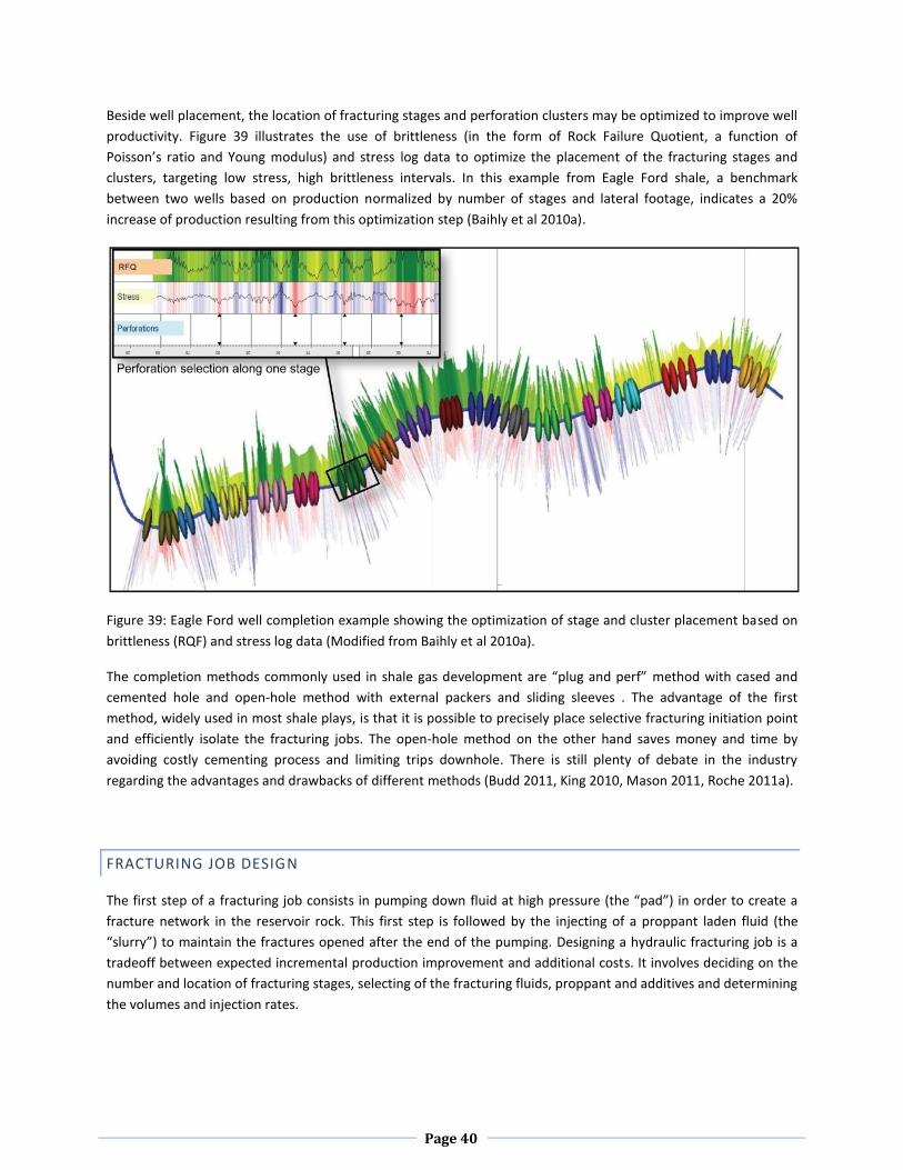
well bore while drilling as well as for placing the fracturing stages and designing the stimulation treatment. Baihly

et al (2010a) illustrates how a better placement of 10 perforation clusters located out of the sweet spot zone might

improve the gross gas revenue by $3 million on a 3 Bcf well, based on $5/Mcf gas price (Fig. 38).

Figure 38: Horizontal well case study in the Woodford shale (Baihly et al 2010a). The well was steered with

conventional gamma ray only. The vertical red bars represent production log values. Clusters located outside the

sweet spot zone in purple provided only minor contribution to the total production.

Page 40

Beside well placement, the location of fracturing stages and perforation clusters may be optimized to improve well

productivity. Figure 39 illustrates the use of brittleness (in the form of Rock Failure Quotient, a function of

Poisson’s ratio and Young modulus) and stress log data to optimize the placement of the fracturing stages and

clusters, targeting low stress, high brittleness intervals. In this example from Eagle Ford shale, a benchmark

between two wells based on production normalized by number of stages and lateral footage, indicates a 20%

increase of production resulting from this optimization step (Baihly et al 2010a).

Figure 39: Eagle Ford well completion example showing the optimization of stage and cluster placement based on

brittleness (RQF) and stress log data (Modified from Baihly et al 2010a).

The completion methods commonly used in shale gas development are “plug and perf” method with cased and

cemented hole and open-hole method with external packers and sliding sleeves . The advantage of the first

method, widely used in most shale plays, is that it is possible to precisely place selective fracturing initiation point

and efficiently isolate the fracturing jobs. The open-hole method on the other hand saves money and time by

avoiding costly cementing process and limiting trips downhole. There is still plenty of debate in the industry

regarding the advantages and drawbacks of different methods (Budd 2011, King 2010, Mason 2011, Roche 2011a).

FRACTURING JOB DESIGN

The first step of a fracturing job consists in pumping down fluid at high pressure (the “pad”) in order to create a

fracture network in the reservoir rock. This first step is followed by the injecting of a proppant laden fluid (the

“slurry”) to maintain the fractures opened after the end of the pumping. Designing a hydraulic fracturing job is a

tradeoff between expected incremental production improvement and additional costs. It involves deciding on the

number and location of fracturing stages, selecting of the fracturing fluids, proppant and additives and determining

the volumes and injection rates.

Page 41

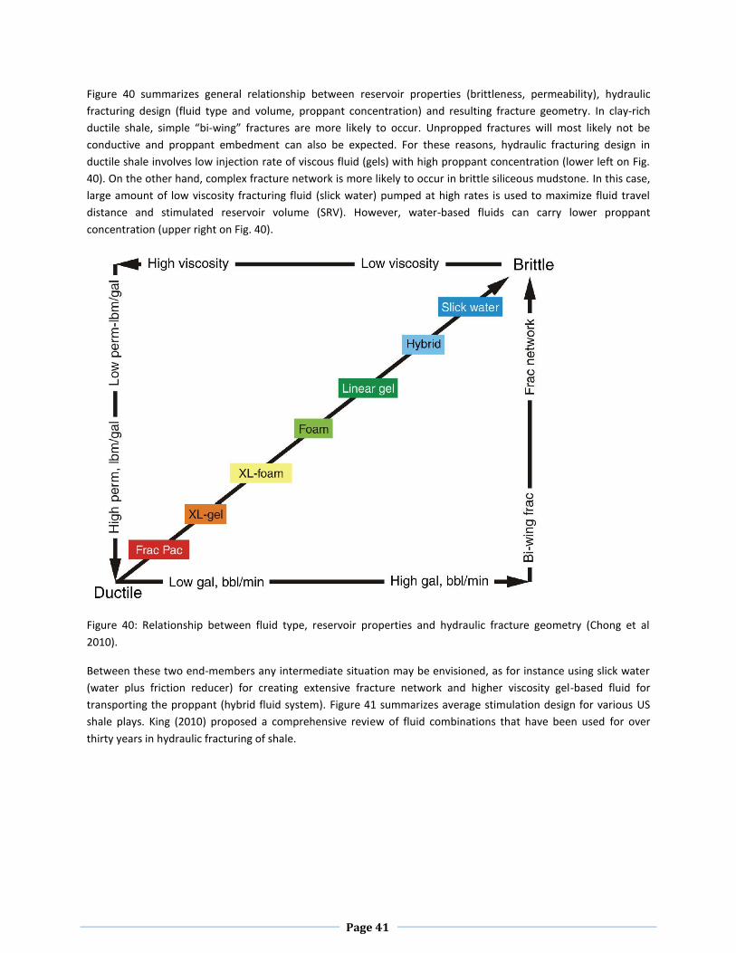
Figure 40 summarizes general relationship between reservoir properties (brittleness, permeability), hydraulic

fracturing design (fluid type and volume, proppant concentration) and resulting fracture geometry. In clay-rich

ductile shale, simple “bi-wing” fractures are more likely to occur. Unpropped fractures will most likely not be

conductive and proppant embedment can also be expected. For these reasons, hydraulic fracturing design in

ductile shale involves low injection rate of viscous fluid (gels) with high proppant concentration (lower left on Fig.

40). On the other hand, complex fracture network is more likely to occur in brittle siliceous mudstone. In this case,

large amount of low viscosity fracturing fluid (slick water) pumped at high rates is used to maximize fluid travel

distance and stimulated reservoir volume (SRV). However, water-based fluids can carry lower proppant

concentration (upper right on Fig. 40).

Figure 40: Relationship between fluid type, reservoir properties and hydraulic fracture geometry (Chong et al

2010).

Between these two end-members any intermediate situation may be envisioned, as for instance using slick water

(water plus friction reducer) for creating extensive fracture network and higher viscosity gel-based fluid for

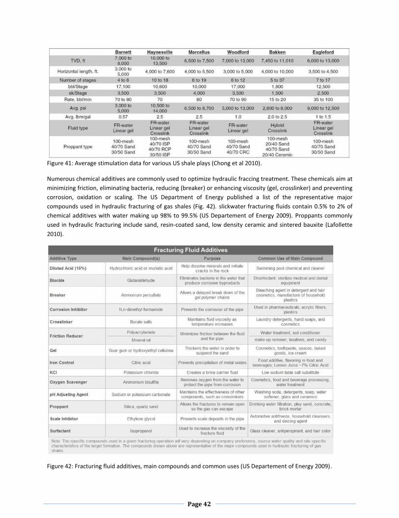
transporting the proppant (hybrid fluid system). Figure 41 summarizes average stimulation design for various US

shale plays. King (2010) proposed a comprehensive review of fluid combinations that have been used for over

thirty years in hydraulic fracturing of shale.

Page 42

Figure 41: Average stimulation data for various US shale plays (Chong et al 2010).

Numerous chemical additives are commonly used to optimize hydraulic fraccing treatment. These chemicals aim at

minimizing friction, eliminating bacteria, reducing (breaker) or enhancing viscosity (gel, crosslinker) and preventing

corrosion, oxidation or scaling. The US Department of Energy published a list of the representative major

compounds used in hydraulic fracturing of gas shales (Fig. 42). slickwater fracturing fluids contain 0.5% to 2% of

chemical additives with water making up 98% to 99.5% (US Departement of Energy 2009). Proppants commonly

used in hydraulic fracturing include sand, resin-coated sand, low density ceramic and sintered bauxite (Lafollette

2010).

Figure 42: Fracturing fluid additives, main compounds and common uses (US Departement of Energy 2009).

Page 43

Critical input parameters needed for hydraulic fracturing design and reservoir models are commonly obtained by

performing pre-frac injection tests, also referred to as minifrac tests. They consist in injecting water, oil or nitrogen

to breakdown the formation and monitoring injection and falloff pressure variation with time. Analysis of pre-frac

test can provide key parameters such as closure pressure, pipe and near-well bore friction losses, fracture

geometry, fluid leakoff coefficient and formation permeability (Barree 2009b, Santo 2011).

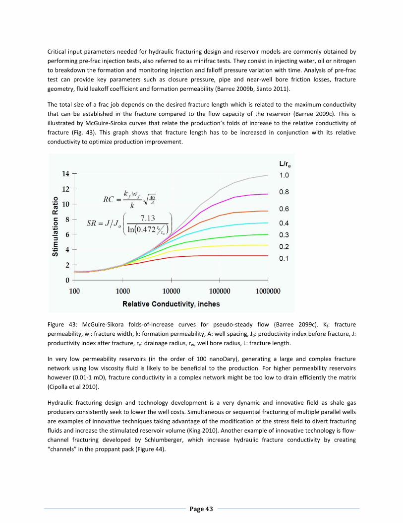
The total size of a frac job depends on the desired fracture length which is related to the maximum conductivity

that can be established in the fracture compared to the flow capacity of the reservoir (Barree 2009c). This is

illustrated by McGuire-Siroka curves that relate the production’s folds of increase to the relative conductivity of

fracture (Fig. 43). This graph shows that fracture length has to be increased in conjunction with its relative

conductivity to optimize production improvement.

Figure 43: McGuire-Sikora folds-of-Increase curves for pseudo-steady flow (Barree 2099c). Kf: fracture

permeability, wf: fracture width, k: formation permeability, A: well spacing, J0: productivity index before fracture, J:

productivity index after fracture, re: drainage radius, rw, well bore radius, L: fracture length.

In very low permeability reservoirs (in the order of 100 nanoDary), generating a large and complex fracture

network using low viscosity fluid is likely to be beneficial to the production. For higher permeability reservoirs

however (0.01-1 mD), fracture conductivity in a complex network might be too low to drain efficiently the matrix

(Cipolla et al 2010).

Hydraulic fracturing design and technology development is a very dynamic and innovative field as shale gas

producers consistently seek to lower the well costs. Simultaneous or sequential fracturing of multiple parallel wells

are examples of innovative techniques taking advantage of the modification of the stress field to divert fracturing

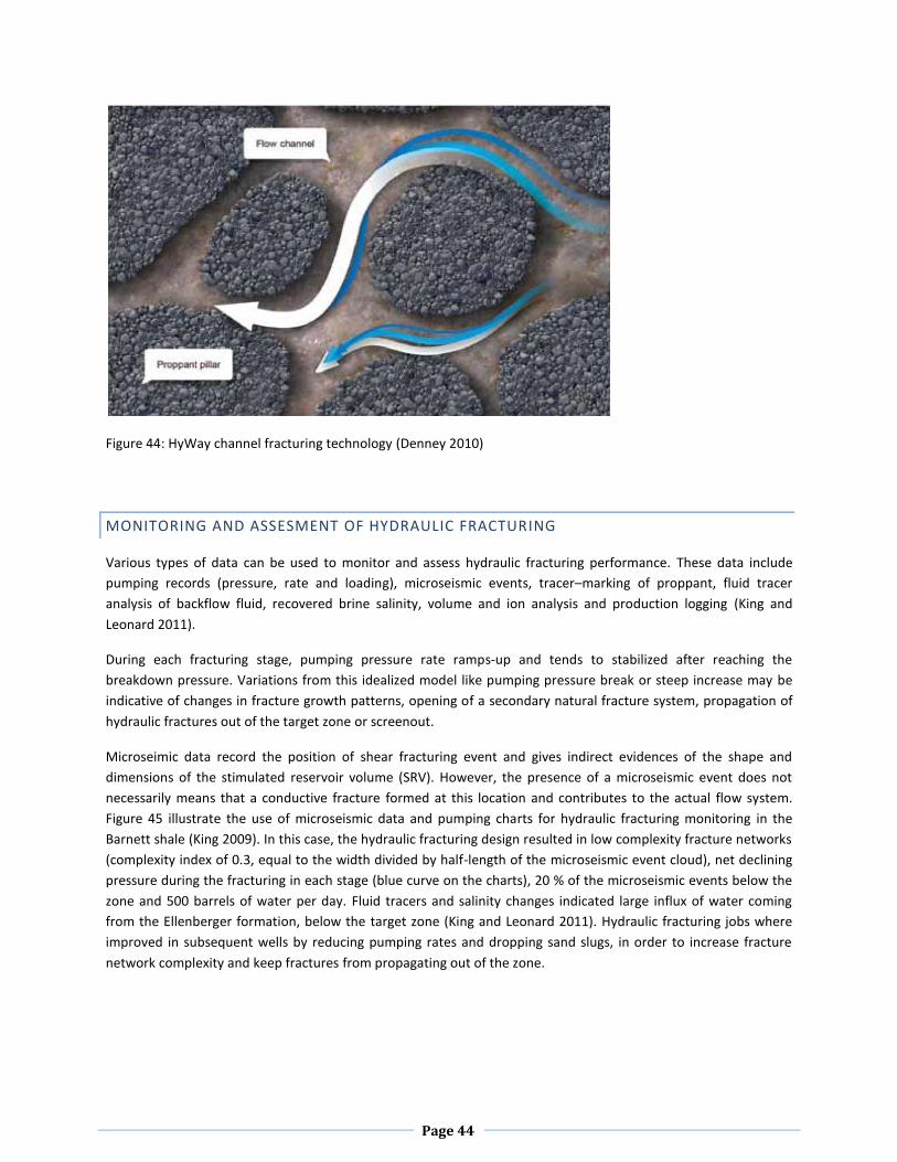
fluids and increase the stimulated reservoir volume (King 2010). Another example of innovative technology is flow-

channel fracturing developed by Schlumberger, which increase hydraulic fracture conductivity by creating

“channels” in the proppant pack (Figure 44).

Page 44

Figure 44: HyWay channel fracturing technology (Denney 2010)

MONITORING AND ASSESMENT OF HYDRAULIC FRACTURING

Various types of data can be used to monitor and assess hydraulic fracturing performance. These data include

pumping records (pressure, rate and loading), microseismic events, tracer–marking of proppant, fluid tracer

analysis of backflow fluid, recovered brine salinity, volume and ion analysis and production logging (King and

Leonard 2011).

During each fracturing stage, pumping pressure rate ramps-up and tends to stabilized after reaching the

breakdown pressure. Variations from this idealized model like pumping pressure break or steep increase may be

indicative of changes in fracture growth patterns, opening of a secondary natural fracture system, propagation of

hydraulic fractures out of the target zone or screenout.

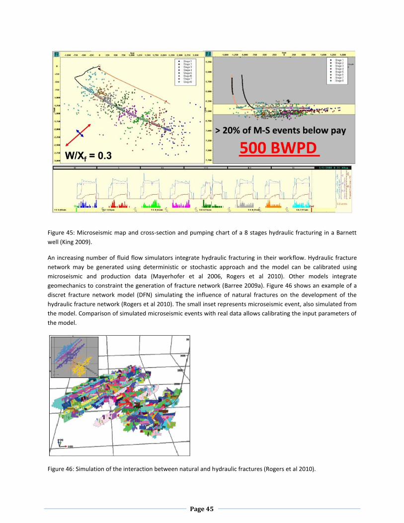
Microseimic data record the position of shear fracturing event and gives indirect evidences of the shape and

dimensions of the stimulated reservoir volume (SRV). However, the presence of a microseismic event does not

necessarily means that a conductive fracture formed at this location and contributes to the actual flow system.

Figure 45 illustrate the use of microseismic data and pumping charts for hydraulic fracturing monitoring in the

Barnett shale (King 2009). In this case, the hydraulic fracturing design resulted in low complexity fracture networks

(complexity index of 0.3, equal to the width divided by half-length of the microseismic event cloud), net declining

pressure during the fracturing in each stage (blue curve on the charts), 20 % of the microseismic events below the

zone and 500 barrels of water per day. Fluid tracers and salinity changes indicated large influx of water coming

from the Ellenberger formation, below the target zone (King and Leonard 2011). Hydraulic fracturing jobs where

improved in subsequent wells by reducing pumping rates and dropping sand slugs, in order to increase fracture

network complexity and keep fractures from propagating out of the zone.

Page 45

Figure 45: Microseismic map and cross-section and pumping chart of a 8 stages hydraulic fracturing in a Barnett

well (King 2009).

An increasing number of fluid flow simulators integrate hydraulic fracturing in their workflow. Hydraulic fracture

network may be generated using deterministic or stochastic approach and the model can be calibrated using

microseismic and production data (Mayerhofer et al 2006, Rogers et al 2010). Other models integrate

geomechanics to constraint the generation of fracture network (Barree 2009a). Figure 46 shows an example of a

discret fracture network model (DFN) simulating the influence of natural fractures on the development of the

hydraulic fracture network (Rogers et al 2010). The small inset represents microseismic event, also simulated from

the model. Comparison of simulated microseismic events with real data allows calibrating the input parameters of

the model.

Figure 46: Simulation of the interaction between natural and hydraulic fractures (Rogers et al 2010).

Page 46

Stimulated reservoir volume (SRV) derived from microseismic data and initial production rates (IP) are good

indicators of hydraulic fracturing efficiency, but only long term production data will ultimately give the final reality

check.

Page 47

SHALE GAS PRODUCTIVITY AND RESOURCE ASSESSMENT

SHALE GAS PRODUCTIVITY

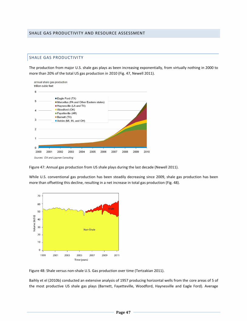
The production from major U.S. shale gas plays as been increasing exponentially, from virtually nothing in 2000 to

more than 20% of the total US gas production in 2010 (Fig. 47, Newell 2011).

Figure 47: Annual gas production from US shale plays during the last decade (Newell 2011).

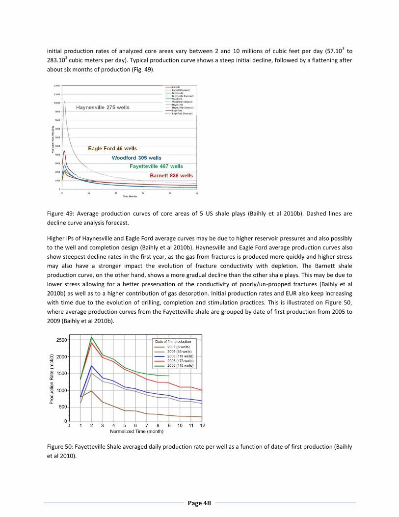
While U.S. conventional gas production has been steadily decreasing since 2009, shale gas production has been

more than offsetting this decline, resulting in a net increase in total gas production (Fig. 48).

Figure 48: Shale versus non-shale U.S. Gas production over time (Tertzakian 2011).

Baihly et el (2010b) conducted an extensive analysis of 1957 producing horizontal wells from the core areas of 5 of

the most productive US shale gas plays (Barnett, Fayetteville, Woodford, Haynesville and Eagle Ford). Average

Page 48

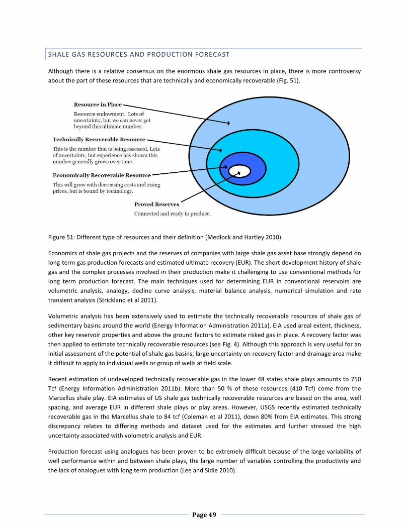
initial production rates of analyzed core areas vary between 2 and 10 millions of cubic feet per day (57.103 to

283.103 cubic meters per day). Typical production curve shows a steep initial decline, followed by a flattening after

about six months of production (Fig. 49).

Figure 49: Average production curves of core areas of 5 US shale plays (Baihly et al 2010b). Dashed lines are

decline curve analysis forecast.

Higher IPs of Haynesville and Eagle Ford average curves may be due to higher reservoir pressures and also possibly

to the well and completion design (Baihly et al 2010b). Haynesville and Eagle Ford average production curves also

show steepest decline rates in the first year, as the gas from fractures is produced more quickly and higher stress

may also have a stronger impact the evolution of fracture conductivity with depletion. The Barnett shale

production curve, on the other hand, shows a more gradual decline than the other shale plays. This may be due to

lower stress allowing for a better preservation of the conductivity of poorly/un-propped fractures (Baihly et al

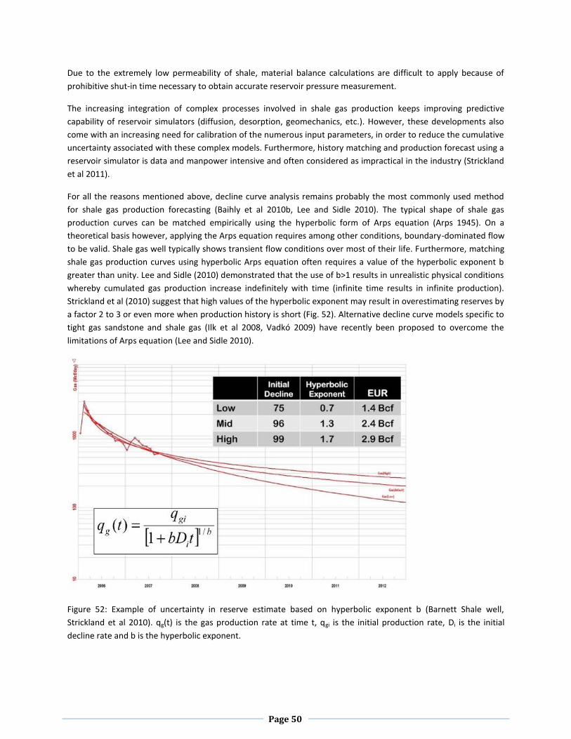
2010b) as well as to a higher contribution of gas desorption. Initial production rates and EUR also keep increasing

with time due to the evolution of drilling, completion and stimulation practices. This is illustrated on Figure 50,

where average production curves from the Fayetteville shale are grouped by date of first production from 2005 to

2009 (Baihly et al 2010b).

Figure 50: Fayetteville Shale averaged daily production rate per well as a function of date of first production (Baihly

et al 2010).

Page 49

SHALE GAS RESOURCES AND PRODUCTION FORECAST

Although there is a relative consensus on the enormous shale gas resources in place, there is more controversy

about the part of these resources that are technically and economically recoverable (Fig. 51).

Figure 51: Different type of resources and their definition (Medlock and Hartley 2010).

Economics of shale gas projects and the reserves of companies with large shale gas asset base strongly depend on

long-term gas production forecasts and estimated ultimate recovery (EUR). The short development history of shale

gas and the complex processes involved in their production make it challenging to use conventional methods for

long term production forecast. The main techniques used for determining EUR in conventional reservoirs are

volumetric analysis, analogy, decline curve analysis, material balance analysis, numerical simulation and rate

transient analysis (Strickland et al 2011).

Volumetric analysis has been extensively used to estimate the technically recoverable resources of shale gas of

sedimentary basins around the world (Energy Information Administration 2011a). EIA used areal extent, thickness,

other key reservoir properties and above the ground factors to estimate risked gas in place. A recovery factor was

then applied to estimate technically recoverable resources (see Fig. 4). Although this approach is very useful for an

initial assessment of the potential of shale gas basins, large uncertainty on recovery factor and drainage area make

it difficult to apply to individual wells or group of wells at field scale.

Recent estimation of undeveloped technically recoverable gas in the lower 48 states shale plays amounts to 750

Tcf (Energy Information Administration 2011b). More than 50 % of these resources (410 Tcf) come from the

Marcellus shale play. EIA estimates of US shale gas technically recoverable resources are based on the area, well

spacing, and average EUR in different shale plays or play areas. However, USGS recently estimated technically

recoverable gas in the Marcellus shale to 84 tcf (Coleman et al 2011), down 80% from EIA estimates. This strong

discrepancy relates to differing methods and dataset used for the estimates and further stressed the high

uncertainty associated with volumetric analysis and EUR.

Production forecast using analogues has been proven to be extremely difficult because of the large variability of

well performance within and between shale plays, the large number of variables controlling the productivity and

the lack of analogues with long term production (Lee and Sidle 2010).

Page 50

Due to the extremely low permeability of shale, material balance calculations are difficult to apply because of

prohibitive shut-in time necessary to obtain accurate reservoir pressure measurement.

The increasing integration of complex processes involved in shale gas production keeps improving predictive

capability of reservoir simulators (diffusion, desorption, geomechanics, etc.). However, these developments also

come with an increasing need for calibration of the numerous input parameters, in order to reduce the cumulative

uncertainty associated with these complex models. Furthermore, history matching and production forecast using a

reservoir simulator is data and manpower intensive and often considered as impractical in the industry (Strickland

et al 2011).

For all the reasons mentioned above, decline curve analysis remains probably the most commonly used method

for shale gas production forecasting (Baihly et al 2010b, Lee and Sidle 2010). The typical shape of shale gas

production curves can be matched empirically using the hyperbolic form of Arps equation (Arps 1945). On a

theoretical basis however, applying the Arps equation requires among other conditions, boundary-dominated flow

to be valid. Shale gas well typically shows transient flow conditions over most of their life. Furthermore, matching

shale gas production curves using hyperbolic Arps equation often requires a value of the hyperbolic exponent b

greater than unity. Lee and Sidle (2010) demonstrated that the use of b>1 results in unrealistic physical conditions

whereby cumulated gas production increase indefinitely with time (infinite time results in infinite production).

Strickland et al (2010) suggest that high values of the hyperbolic exponent may result in overestimating reserves by

a factor 2 to 3 or even more when production history is short (Fig. 52). Alternative decline curve models specific to

tight gas sandstone and shale gas (Ilk et al 2008, Vadkó 2009) have recently been proposed to overcome the

limitations of Arps equation (Lee and Sidle 2010).

Figure 52: Example of uncertainty in reserve estimate based on hyperbolic exponent b (Barnett Shale well,

Strickland et al 2010). qg(t) is the gas production rate at time t, qgi is the initial production rate, Di is the initial

decline rate and b is the hyperbolic exponent.

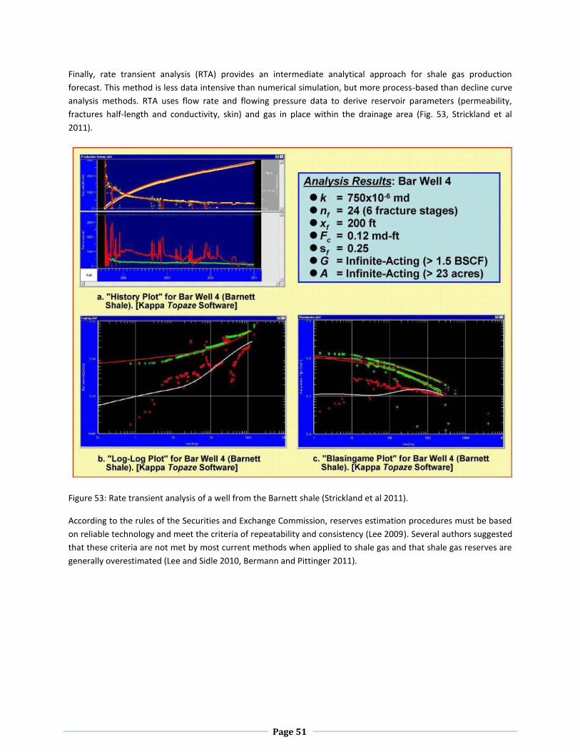
Page 51

Finally, rate transient analysis (RTA) provides an intermediate analytical approach for shale gas production

forecast. This method is less data intensive than numerical simulation, but more process-based than decline curve

analysis methods. RTA uses flow rate and flowing pressure data to derive reservoir parameters (permeability,

fractures half-length and conductivity, skin) and gas in place within the drainage area (Fig. 53, Strickland et al

2011).

Figure 53: Rate transient analysis of a well from the Barnett shale (Strickland et al 2011).

According to the rules of the Securities and Exchange Commission, reserves estimation procedures must be based

on reliable technology and meet the criteria of repeatability and consistency (Lee 2009). Several authors suggested

that these criteria are not met by most current methods when applied to shale gas and that shale gas reserves are

generally overestimated (Lee and Sidle 2010, Bermann and Pittinger 2011).

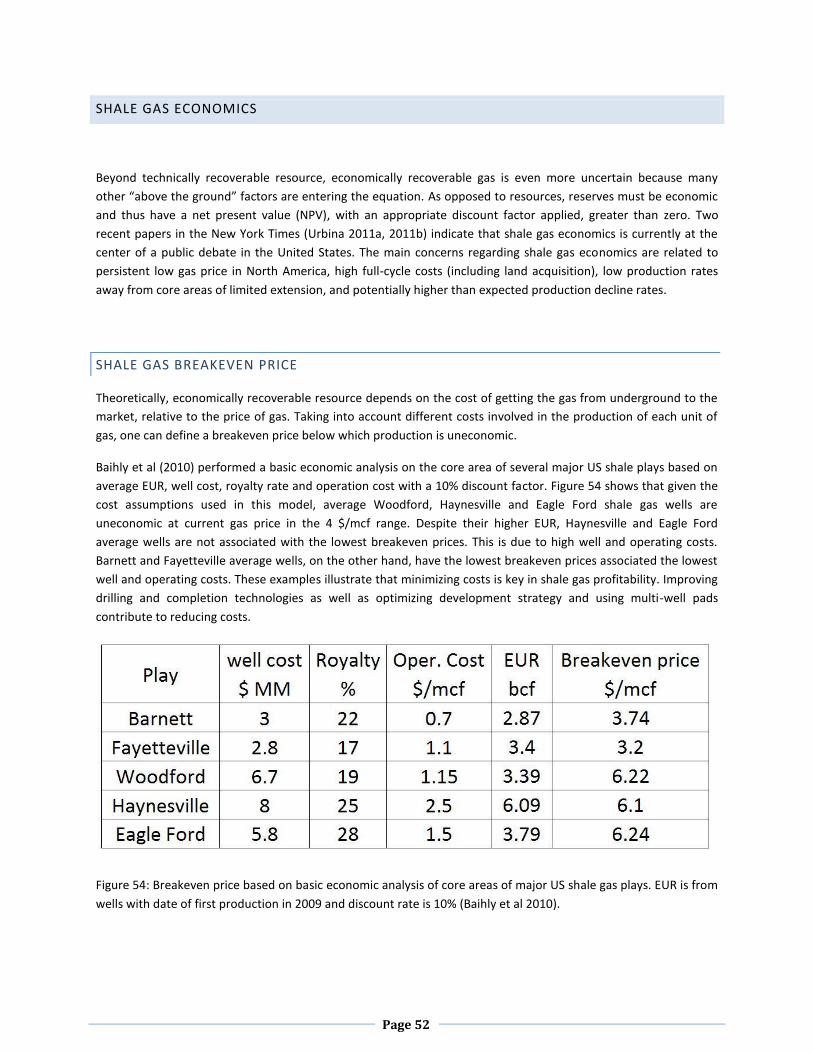
Page 52

SHALE GAS ECONOMICS

Beyond technically recoverable resource, economically recoverable gas is even more uncertain because many

other “above the ground” factors are entering the equation. As opposed to resources, reserves must be economic

and thus have a net present value (NPV), with an appropriate discount factor applied, greater than zero. Two

recent papers in the New York Times (Urbina 2011a, 2011b) indicate that shale gas economics is currently at the

center of a public debate in the United States. The main concerns regarding shale gas economics are related to

persistent low gas price in North America, high full-cycle costs (including land acquisition), low production rates

away from core areas of limited extension, and potentially higher than expected production decline rates.

SHALE GAS BREAKEVEN PRICE

Theoretically, economically recoverable resource depends on the cost of getting the gas from underground to the

market, relative to the price of gas. Taking into account different costs involved in the production of each unit of

gas, one can define a breakeven price below which production is uneconomic.

Baihly et al (2010) performed a basic economic analysis on the core area of several major US shale plays based on

average EUR, well cost, royalty rate and operation cost with a 10% discount factor. Figure 54 shows that given the

cost assumptions used in this model, average Woodford, Haynesville and Eagle Ford shale gas wells are

uneconomic at current gas price in the 4 $/mcf range. Despite their higher EUR, Haynesville and Eagle Ford

average wells are not associated with the lowest breakeven prices. This is due to high well and operating costs.

Barnett and Fayetteville average wells, on the other hand, have the lowest breakeven prices associated the lowest

well and operating costs. These examples illustrate that minimizing costs is key in shale gas profitability. Improving

drilling and completion technologies as well as optimizing development strategy and using multi-well pads

contribute to reducing costs.

Figure 54: Breakeven price based on basic economic analysis of core areas of major US shale gas plays. EUR is from

wells with date of first production in 2009 and discount rate is 10% (Baihly et al 2010).

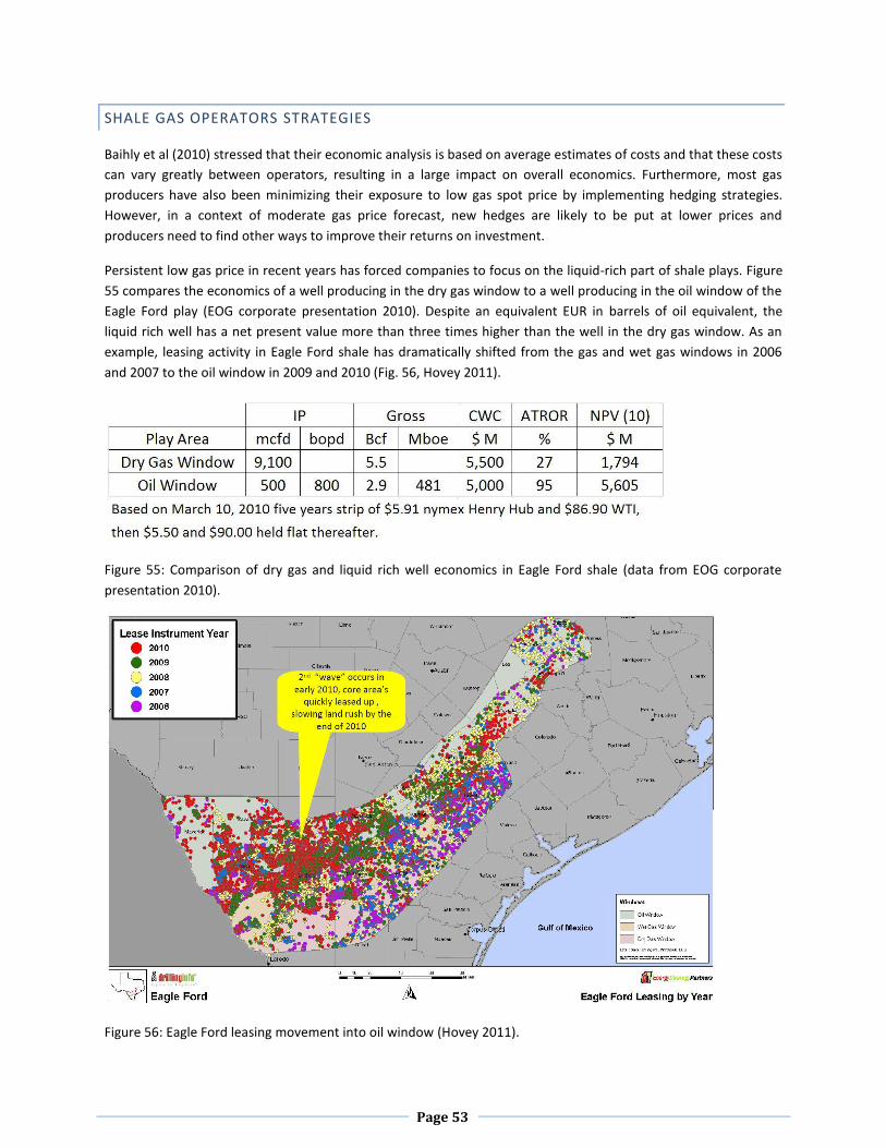
Page 53

SHALE GAS OPERATORS STRATEGIES

Baihly et al (2010) stressed that their economic analysis is based on average estimates of costs and that these costs

can vary greatly between operators, resulting in a large impact on overall economics. Furthermore, most gas

producers have also been minimizing their exposure to low gas spot price by implementing hedging strategies.

However, in a context of moderate gas price forecast, new hedges are likely to be put at lower prices and

producers need to find other ways to improve their returns on investment.

Persistent low gas price in recent years has forced companies to focus on the liquid-rich part of shale plays. Figure

55 compares the economics of a well producing in the dry gas window to a well producing in the oil window of the

Eagle Ford play (EOG corporate presentation 2010). Despite an equivalent EUR in barrels of oil equivalent, the

liquid rich well has a net present value more than three times higher than the well in the dry gas window. As an

example, leasing activity in Eagle Ford shale has dramatically shifted from the gas and wet gas windows in 2006

and 2007 to the oil window in 2009 and 2010 (Fig. 56, Hovey 2011).

Figure 55: Comparison of dry gas and liquid rich well economics in Eagle Ford shale (data from EOG corporate

presentation 2010).

Figure 56: Eagle Ford leasing movement into oil window (Hovey 2011).

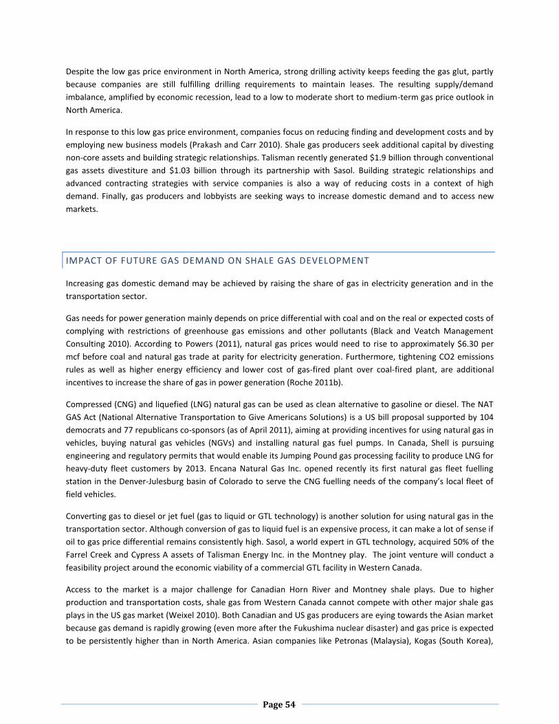
Page 54

Despite the low gas price environment in North America, strong drilling activity keeps feeding the gas glut, partly

because companies are still fulfilling drilling requirements to maintain leases. The resulting supply/demand

imbalance, amplified by economic recession, lead to a low to moderate short to medium-term gas price outlook in

North America.

In response to this low gas price environment, companies focus on reducing finding and development costs and by

employing new business models (Prakash and Carr 2010). Shale gas producers seek additional capital by divesting

non-core assets and building strategic relationships. Talisman recently generated $1.9 billion through conventional

gas assets divestiture and $1.03 billion through its partnership with Sasol. Building strategic relationships and

advanced contracting strategies with service companies is also a way of reducing costs in a context of high

demand. Finally, gas producers and lobbyists are seeking ways to increase domestic demand and to access new

markets.

IMPACT OF FUTURE GAS DEMAND ON SHALE GAS DEVELOPMENT

Increasing gas domestic demand may be achieved by raising the share of gas in electricity generation and in the

transportation sector.

Gas needs for power generation mainly depends on price differential with coal and on the real or expected costs of

complying with restrictions of greenhouse gas emissions and other pollutants (Black and Veatch Management

Consulting 2010). According to Powers (2011), natural gas prices would need to rise to approximately $6.30 per

mcf before coal and natural gas trade at parity for electricity generation. Furthermore, tightening CO2 emissions

rules as well as higher energy efficiency and lower cost of gas-fired plant over coal-fired plant, are additional

incentives to increase the share of gas in power generation (Roche 2011b).

Compressed (CNG) and liquefied (LNG) natural gas can be used as clean alternative to gasoline or diesel. The NAT

GAS Act (National Alternative Transportation to Give Americans Solutions) is a US bill proposal supported by 104

democrats and 77 republicans co-sponsors (as of April 2011), aiming at providing incentives for using natural gas in

vehicles, buying natural gas vehicles (NGVs) and installing natural gas fuel pumps. In Canada, Shell is pursuing

engineering and regulatory permits that would enable its Jumping Pound gas processing facility to produce LNG for

heavy-duty fleet customers by 2013. Encana Natural Gas Inc. opened recently its first natural gas fleet fuelling

station in the Denver-Julesburg basin of Colorado to serve the CNG fuelling needs of the company’s local fleet of

field vehicles.

Converting gas to diesel or jet fuel (gas to liquid or GTL technology) is another solution for using natural gas in the

transportation sector. Although conversion of gas to liquid fuel is an expensive process, it can make a lot of sense if

oil to gas price differential remains consistently high. Sasol, a world expert in GTL technology, acquired 50% of the

Farrel Creek and Cypress A assets of Talisman Energy Inc. in the Montney play. The joint venture will conduct a

feasibility project around the economic viability of a commercial GTL facility in Western Canada.

Access to the market is a major challenge for Canadian Horn River and Montney shale plays. Due to higher

production and transportation costs, shale gas from Western Canada cannot compete with other major shale gas

plays in the US gas market (Weixel 2010). Both Canadian and US gas producers are eying towards the Asian market

because gas demand is rapidly growing (even more after the Fukushima nuclear disaster) and gas price is expected

to be persistently higher than in North America. Asian companies like Petronas (Malaysia), Kogas (South Korea),

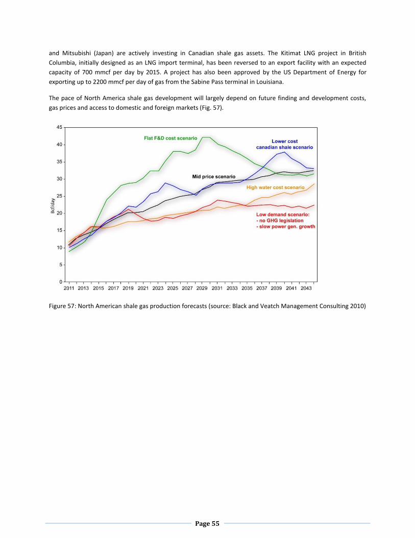
Page 55

and Mitsubishi (Japan) are actively investing in Canadian shale gas assets. The Kitimat LNG project in British

Columbia, initially designed as an LNG import terminal, has been reversed to an export facility with an expected

capacity of 700 mmcf per day by 2015. A project has also been approved by the US Department of Energy for

exporting up to 2200 mmcf per day of gas from the Sabine Pass terminal in Louisiana.

The pace of North America shale gas development will largely depend on future finding and development costs,

gas prices and access to domestic and foreign markets (Fig. 57).

Figure 57: North American shale gas production forecasts (source: Black and Veatch Management Consulting 2010)

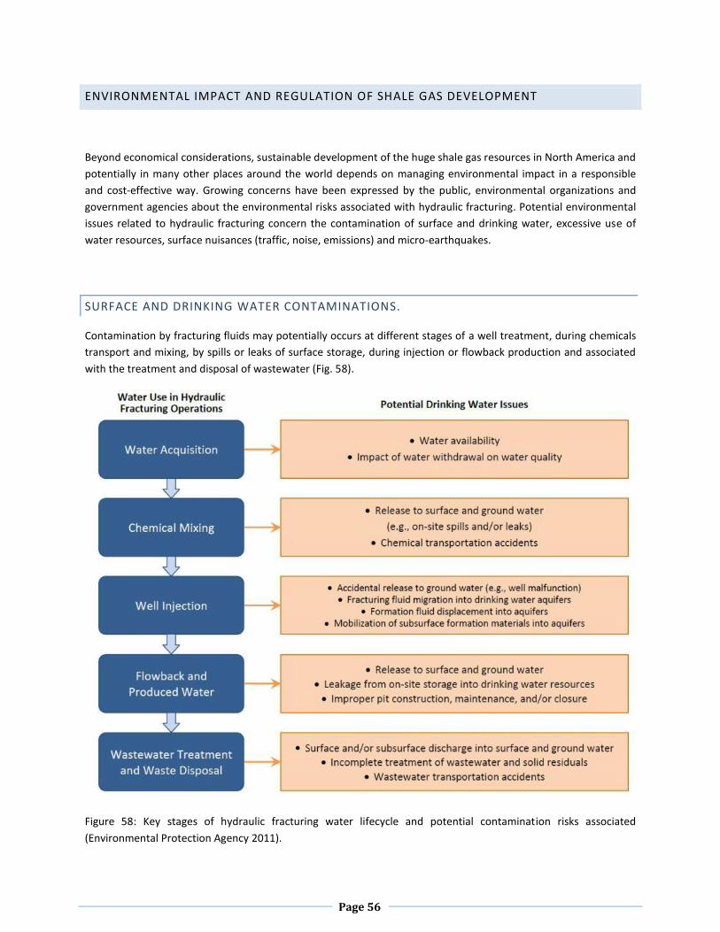
Page 56

ENVIRONMENTAL IMPACT AND REGULATION OF SHALE GAS DEVELOPMENT

Beyond economical considerations, sustainable development of the huge shale gas resources in North America and

potentially in many other places around the world depends on managing environmental impact in a responsible

and cost-effective way. Growing concerns have been expressed by the public, environmental organizations and

government agencies about the environmental risks associated with hydraulic fracturing. Potential environmental

issues related to hydraulic fracturing concern the contamination of surface and drinking water, excessive use of

water resources, surface nuisances (traffic, noise, emissions) and micro-earthquakes.

SURFACE AND DRINKING WATER CONTAMINATIONS.

Contamination by fracturing fluids may potentially occurs at different stages of a well treatment, during chemicals

transport and mixing, by spills or leaks of surface storage, during injection or flowback production and associated

with the treatment and disposal of wastewater (Fig. 58).

Figure 58: Key stages of hydraulic fracturing water lifecycle and potential contamination risks associated

(Environmental Protection Agency 2011).

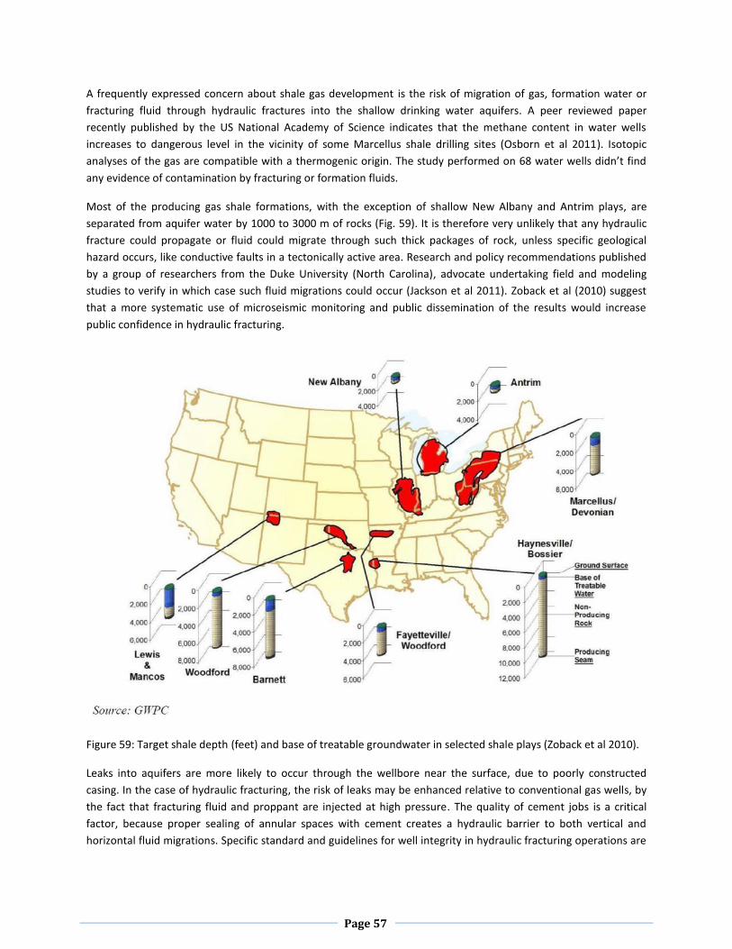
Page 57

A frequently expressed concern about shale gas development is the risk of migration of gas, formation water or

fracturing fluid through hydraulic fractures into the shallow drinking water aquifers. A peer reviewed paper

recently published by the US National Academy of Science indicates that the methane content in water wells

increases to dangerous level in the vicinity of some Marcellus shale drilling sites (Osborn et al 2011). Isotopic

analyses of the gas are compatible with a thermogenic origin. The study performed on 68 water wells didn’t find

any evidence of contamination by fracturing or formation fluids.

Most of the producing gas shale formations, with the exception of shallow New Albany and Antrim plays, are

separated from aquifer water by 1000 to 3000 m of rocks (Fig. 59). It is therefore very unlikely that any hydraulic

fracture could propagate or fluid could migrate through such thick packages of rock, unless specific geological

hazard occurs, like conductive faults in a tectonically active area. Research and policy recommendations published

by a group of researchers from the Duke University (North Carolina), advocate undertaking field and modeling

studies to verify in which case such fluid migrations could occur (Jackson et al 2011). Zoback et al (2010) suggest

that a more systematic use of microseismic monitoring and public dissemination of the results would increase

public confidence in hydraulic fracturing.

Figure 59: Target shale depth (feet) and base of treatable groundwater in selected shale plays (Zoback et al 2010).

Leaks into aquifers are more likely to occur through the wellbore near the surface, due to poorly constructed

casing. In the case of hydraulic fracturing, the risk of leaks may be enhanced relative to conventional gas wells, by

the fact that fracturing fluid and proppant are injected at high pressure. The quality of cement jobs is a critical

factor, because proper sealing of annular spaces with cement creates a hydraulic barrier to both vertical and

horizontal fluid migrations. Specific standard and guidelines for well integrity in hydraulic fracturing operations are

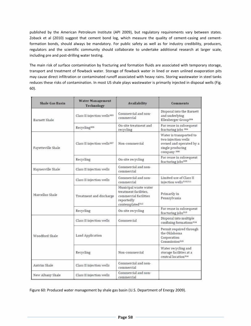
Page 58

published by the American Petroleum Institute (API 2009), but regulatory requirements vary between states.

Zoback et al (2010) suggest that cement bond log, which measure the quality of cement-casing and cement-

formation bonds, should always be mandatory. For public safety as well as for industry credibility, producers,

regulators and the scientific community should collaborate to undertake additional research at larger scale,

including pre and post-drilling water testing.

The main risk of surface contamination by fracturing and formation fluids are associated with temporary storage,

transport and treatment of flowback water. Storage of flowback water in lined or even unlined evaporation pits

may cause direct infiltration or contaminated runoff associated with heavy rains. Storing wastewater in steel tanks

reduces these risks of contamination. In most US shale plays wastewater is primarily injected in disposal wells (Fig.

60).

Figure 60: Produced water management by shale gas basin (U.S. Department of Energy 2009).

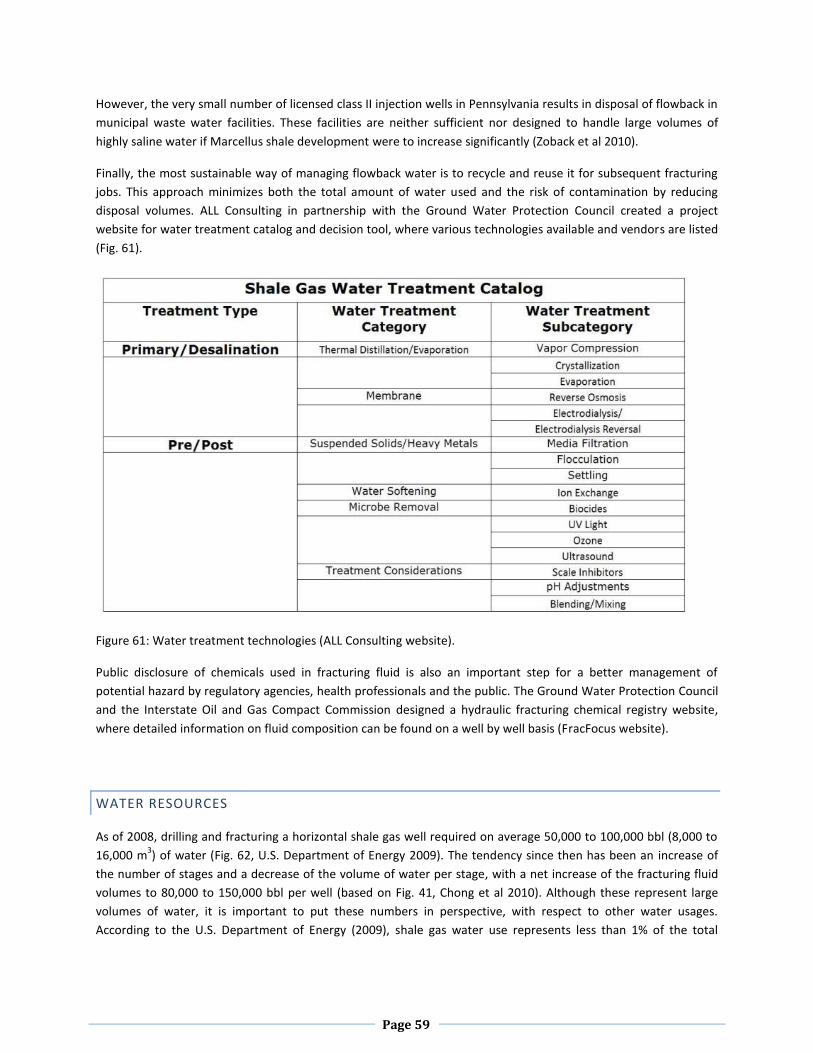
Page 59

However, the very small number of licensed class II injection wells in Pennsylvania results in disposal of flowback in

municipal waste water facilities. These facilities are neither sufficient nor designed to handle large volumes of

highly saline water if Marcellus shale development were to increase significantly (Zoback et al 2010).

Finally, the most sustainable way of managing flowback water is to recycle and reuse it for subsequent fracturing

jobs. This approach minimizes both the total amount of water used and the risk of contamination by reducing

disposal volumes. ALL Consulting in partnership with the Ground Water Protection Council created a project

website for water treatment catalog and decision tool, where various technologies available and vendors are listed

(Fig. 61).

Figure 61: Water treatment technologies (ALL Consulting website).

Public disclosure of chemicals used in fracturing fluid is also an important step for a better management of

potential hazard by regulatory agencies, health professionals and the public. The Ground Water Protection Council

and the Interstate Oil and Gas Compact Commission designed a hydraulic fracturing chemical registry website,

where detailed information on fluid composition can be found on a well by well basis (FracFocus website).

WATER RESOURCES

As of 2008, drilling and fracturing a horizontal shale gas well required on average 50,000 to 100,000 bbl (8,000 to

16,000 m3) of water (Fig. 62, U.S. Department of Energy 2009). The tendency since then has been an increase of

the number of stages and a decrease of the volume of water per stage, with a net increase of the fracturing fluid

volumes to 80,000 to 150,000 bbl per well (based on Fig. 41, Chong et al 2010). Although these represent large

volumes of water, it is important to put these numbers in perspective, with respect to other water usages.

According to the U.S. Department of Energy (2009), shale gas water use represents less than 1% of the total

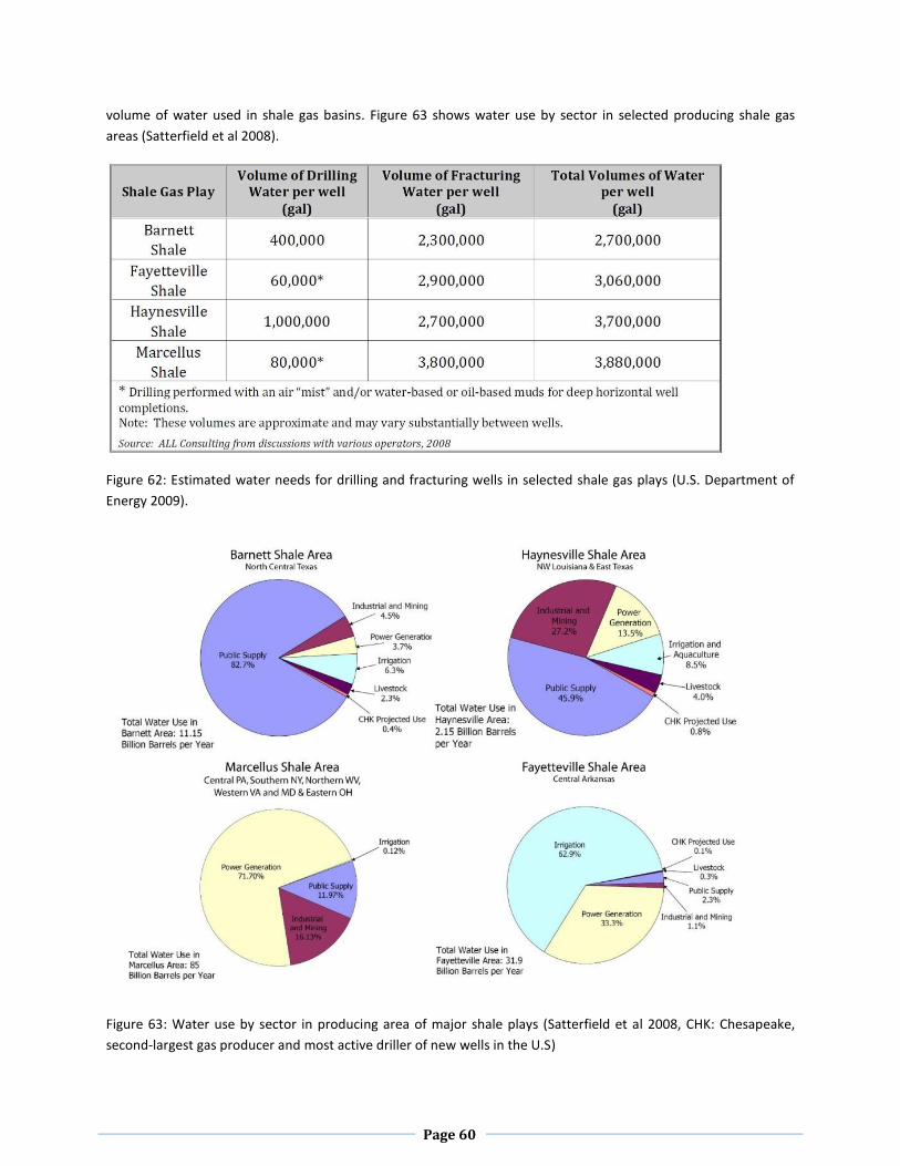
Page 60

volume of water used in shale gas basins. Figure 63 shows water use by sector in selected producing shale gas

areas (Satterfield et al 2008).

Figure 62: Estimated water needs for drilling and fracturing wells in selected shale gas plays (U.S. Department of

Energy 2009).

Figure 63: Water use by sector in producing area of major shale plays (Satterfield et al 2008, CHK: Chesapeake,

second-largest gas producer and most active driller of new wells in the U.S)

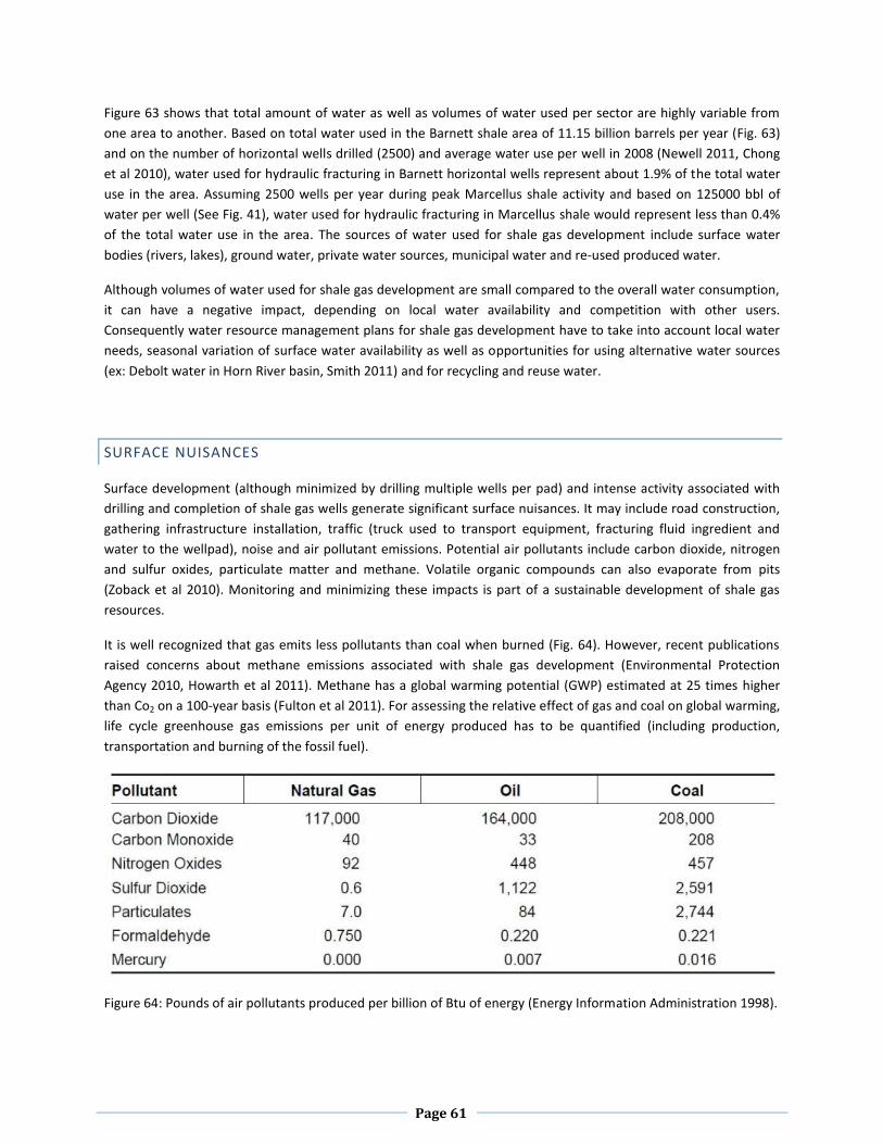
Page 61

Figure 63 shows that total amount of water as well as volumes of water used per sector are highly variable from

one area to another. Based on total water used in the Barnett shale area of 11.15 billion barrels per year (Fig. 63)

and on the number of horizontal wells drilled (2500) and average water use per well in 2008 (Newell 2011, Chong

et al 2010), water used for hydraulic fracturing in Barnett horizontal wells represent about 1.9% of the total water

use in the area. Assuming 2500 wells per year during peak Marcellus shale activity and based on 125000 bbl of

water per well (See Fig. 41), water used for hydraulic fracturing in Marcellus shale would represent less than 0.4%

of the total water use in the area. The sources of water used for shale gas development include surface water

bodies (rivers, lakes), ground water, private water sources, municipal water and re-used produced water.

Although volumes of water used for shale gas development are small compared to the overall water consumption,

it can have a negative impact, depending on local water availability and competition with other users.

Consequently water resource management plans for shale gas development have to take into account local water

needs, seasonal variation of surface water availability as well as opportunities for using alternative water sources

(ex: Debolt water in Horn River basin, Smith 2011) and for recycling and reuse water.

SURFACE NUISANCES

Surface development (although minimized by drilling multiple wells per pad) and intense activity associated with

drilling and completion of shale gas wells generate significant surface nuisances. It may include road construction,

gathering infrastructure installation, traffic (truck used to transport equipment, fracturing fluid ingredient and

water to the wellpad), noise and air pollutant emissions. Potential air pollutants include carbon dioxide, nitrogen

and sulfur oxides, particulate matter and methane. Volatile organic compounds can also evaporate from pits

(Zoback et al 2010). Monitoring and minimizing these impacts is part of a sustainable development of shale gas

resources.

It is well recognized that gas emits less pollutants than coal when burned (Fig. 64). However, recent publications

raised concerns about methane emissions associated with shale gas development (Environmental Protection

Agency 2010, Howarth et al 2011). Methane has a global warming potential (GWP) estimated at 25 times higher

than Co2 on a 100-year basis (Fulton et al 2011). For assessing the relative effect of gas and coal on global warming,

life cycle greenhouse gas emissions per unit of energy produced has to be quantified (including production,

transportation and burning of the fossil fuel).

Figure 64: Pounds of air pollutants produced per billion of Btu of energy (Energy Information Administration 1998).

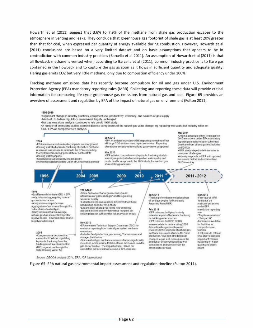
Page 62

Howarth et al (2011) suggest that 3.6% to 7.9% of the methane from shale gas production escapes to the

atmosphere in venting and leaks. They conclude that greenhouse gas footprint of shale gas is at least 20% greater

than that for coal, when expressed per quantity of energy available during combustion. However, Howarth et al

(2011) conclusions are based on a very limited dataset and on basic assumptions that appears to be in

contradiction with common industry practices (Barcella et al 2011). An assumption of Howarth et al (2011) is that

all flowback methane is vented when, according to Barcella et al (2011), common industry practice is to flare gas

contained in the flowback and to capture the gas as soon as it flows in sufficient quantity and adequate quality.

Flaring gas emits CO2 but very little methane, only due to combustion efficiency under 100%.

Tracking methane emissions data has recently become compulsory for oil and gas under U.S. Environment

Protection Agency (EPA) mandatory reporting rules (MRR). Collecting and reporting these data will provide critical

information for comparing life cycle greenhouse gas emissions from natural gas and coal. Figure 65 provides an

overview of assessment and regulation by EPA of the impact of natural gas on environment (Fulton 2011).

Figure 65: EPA natural gas environmental impact assessment and regulation timeline (Fulton 2011).

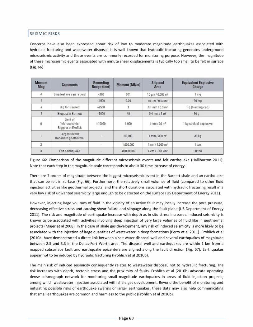
Page 63

SEISMIC RISKS

Concerns have also been expressed about risk of low to moderate magnitude earthquakes associated with

hydraulic fracturing and wastewater disposal. It is well known that hydraulic fracturing generates underground

microseismic activity and these events are commonly recorded for monitoring purpose. However, the magnitude

of these microseismic events associated with minute shear displacements is typically too small to be felt in surface

(Fig. 66)

Figure 66: Comparison of the magnitude different microseismic events and felt earthquake (Halliburton 2011).

Note that each step in the magnitude scale corresponds to about 30 time increase of energy.

There are 7 orders of magnitude between the biggest microseismic event in the Barnett shale and an earthquake

that can be felt in surface (Fig. 66). Furthermore, the relatively small volumes of fluid (compared to other fluid

injection activities like geothermal projects) and the short durations associated with hydraulic fracturing result in a

very low risk of unwanted seismicity large enough to be detected on the surface (US Department of Energy 2011).

However, injecting large volumes of fluid in the vicinity of an active fault may locally increase the pore pressure,

decreasing effective stress and causing shear failure and slippage along the fault plane (US Department of Energy

2011). The risk and magnitude of earthquake increase with depth as in situ stress increases. Induced seismicity is

known to be associated with activities involving deep injection of very large volumes of fluid like in geothermal

projects (Majer et al 2008). In the case of shale gas development, any risk of induced seismicity is more likely to be

associated with the injection of large quantities of wastewater in deep formations (Perry et al 2011). Frohlich et al

(2010a) have demonstrated a direct link between a salt water disposal well and several earthquakes of magnitude

between 2.5 and 3.3 in the Dallas-Fort Worth area. The disposal well and earthquakes are within 1 km from a

mapped subsurface fault and earthquake epicenters are aligned along the fault direction (Fig. 67). Earthquakes

appear not to be induced by hydraulic fracturing (Frohlich et al 2010b).

The main risk of induced seismicity consequently relates to wastewater disposal, not to hydraulic fracturing. The

risk increases with depth, tectonic stress and the proximity of faults. Frohlich et al (2010b) advocate operating

dense seismograph network for monitoring small magnitude earthquakes in areas of fluid injection projects,

among which wastewater injection associated with shale gas development. Beyond the benefit of monitoring and

mitigating possible risks of earthquake swarms or larger earthquakes, these data may also help communicating

that small earthquakes are common and harmless to the public (Frohlich et al 2010b).

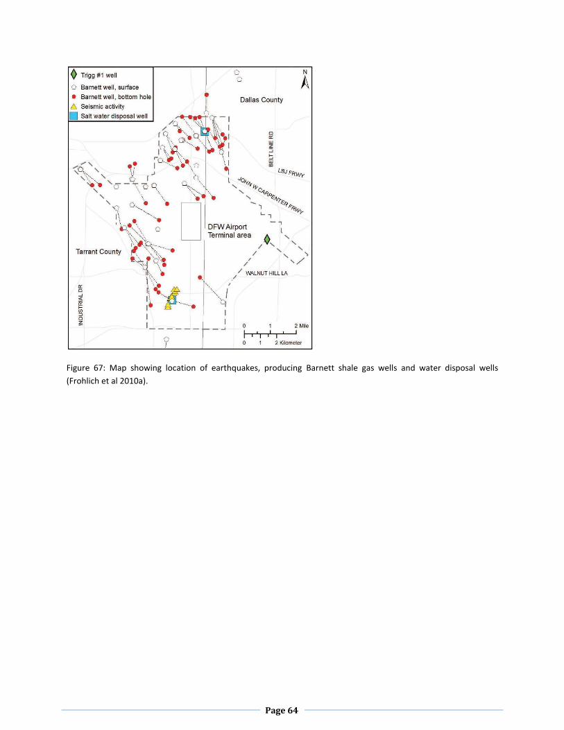
Page 64

Figure 67: Map showing location of earthquakes, producing Barnett shale gas wells and water disposal wells

(Frohlich et al 2010a).

Page 65

CONCLUSION: THE ROLE OF SHALE GAS IN THE FUTURE ENERGY MIX

There is a general consensus on the fact that organic shale hold enormous amount of gas in North America and

potentially in many countries around the world. Whether these huge resources can and will be produced is

however highly uncertain and depends on many factors. The development of the Barnett shale and other emerging

shale plays in North America has demonstrated that horizontal drilling and multistage hydraulic fracturing make it

technically possible to extract large amounts of gas from shale. Today, shale gas production accounts for more

than 20% of the total US gas production.

Growing amount of data and the past successes and failures of the industry have demonstrated that shale

characteristics are highly variable, both between and within plays. Moreover, the prospectivity of shale depends

on numerous controlling factors that vary spatially from nanometer to basin scale. In the first part of this report,

we have seen that several parameters that are not involved in the assessment of most conventional plays have to

be analyzed and integrated in shale gas evaluation. Among those parameters are the organic matter content and

maturity, adsorption capacity, rock elastic properties and in situ stress. Recent advances in high resolution imaging

techniques have demonstrated that vast amounts of gas are trapped in micropores of organic matter in shale. As a

result, reservoir simulators and lab analytical models have to account for adsorption effect and non-darcy flow

processes. Adsorption capacity evaluation is needed to quantify gas in place and better predict long term

productivity. Quantifying shale mineralogy is also paramount because it impacts pore network structure, elastic

properties, fluid sensitivity and log response of shale. Knowledge of rock elastic properties, in situ stress and

natural fractures orientation and density is required to properly design the well and hydraulic fracturing job. In the

recent years, thanks to the contribution of hundreds of technical papers from producers, service companies and

academia, the industry acknowledged the complexity of shale plays and developed a variety specific evaluation

tools and approaches. As a result, shale gas producers have become more efficient in defining porspective areas

and designing well and completion strategies.

Horizontal well drilling and stimulation technologies and practices have been evolving at a fast pace, contributing

to an overall increase of initial production rates (IP) and estimated ultimate recovery (EUR) of gas shale. In

particular, geosteering using LWD, advanced log suits (shale expert systems) and microseismic monitoring

contribute to optimizing the placement of the well and fracturing stages. Various combinations of fluids, additives

and proppant are designed for specific areas and plays, depending on shale composition, mechanical properties,

pore pressure and in situ stress. Recent technology innovations also aim at improving fracture and near wellbore

conductivity and flowback recovery. Different combinations of multiple wells stimulation design including

sequential and simultaneous fracturing are implemented to increase the stimulated reservoir volume.

Overall, improving understanding of shale gas plays and technological innovations have proven the technical ability

of the industry to tap in the very large shale gas resources. However, the shale gas industry is facing a greater

challenge when it comes to economics and environmental issues. Starting in 2008, the combination of economic

recession and exponential increase of shale gas production in United States resulted in oversupplied market and

low gas price. Surprisingly, shale gas production has been increasing consistently since then, despite sustained low

gas price below 5 $/mcf. At current spot gas price (Henry Hub below 4 $/mcf as of September 2011), the most part

of shale gas plays are marginally to not economic. Shale gas producers have been mitigating the effect of low gas

price by optimizing well and operating costs, implementing hedging strategies and by focusing on liquid rich parts

of the plays. Companies are also divesting non-core assets to provide additional capital and improve their balance

Page 66

sheet. Despite the current debate on shale gas economics, huge investments made by major companies in land

positions, joint-ventures and acquisitions, demonstrate that shale gas is part of their long-term strategy.

On the longer term, gas demand increase will be necessary to allows for the full development of North American

shale gas plays and the gas industry is seeking for new markets. Domestic demand will largely depend on public

policies and incentives regarding the use of gas in power generation and transportation sectors. Due to growing

demand and higher price, the Asian gas market can be an important part of the future of North American shale

gas. Asian companies are actively investing in North American shale gas assets while producers are seeking for

government approval for LNG export projects.

A major impediment of future shale gas development in North America and even more adversely in other part of

the world is related to the public perception and environmental issues associated with hydraulic fracturing.

Sustainable development of shale gas resources depends on responsible and cost-effective management of

environmental risks. Proactive collaboration of the industry with regulatory agencies and academia to understand

and mitigate risks associated with surface and drinking water contaminations, flowback disposal and water

resource management will be paramount. Disseminating the results of this research and educating the public can

contribute to alleviate negative perception of shale gas by the public.

Current estimations of global shale gas resources represent about 30% of the world technically recoverable gas

and are widely dispersed geographically. The development of shale gas has the potential to improve energy

security in many areas around the world. According to the International Energy Agency, the share of gas in the

global energy mix might increase by 50% from 2010 to 2035, to represent more than 25% of the world energy

demand (International Energy Agency 2011). In this “high gas” scenario, natural gas-fired generation is expected to

push the share of coal into decline and to back up increasing intermittent renewable sources of electricity. A lower

growth of nuclear power after the Fukushima accident would also favor an increasing share of gas to reduce green

house gas emissions. Increasing gas demand in the transportation sector may also be part of a low carbon future. If

shale gas development is proven to be environmentally and economically sustainable and gains large public

acceptance, it will play a major role in the future global energy mix.

Page 67

REFERENCES

Ambrose, R., Hartman, R., Diaz Campos, M., Akkutlu, I. Y., & Sondergeld, C. (2010). New Pore-scale

Considerations for Shale Gas in Place Calculations. Proceedings of SPE Unconventional Gas Conference,

Pittsburgh, Pennsylvania, USA, 23-25 February 2010. Society of Petroleum Engineers. doi:10.2118/131772-

MS

Anderson S.D.A. , Rokosh C.D., Pawlowicz J.G., B. H. and B. A. P. (2010). Mineralogy, Permeametry, Mercury

Porosimetry, Pycnometry and Scanning Electron Microscope Imaging of the Montney Formation in Alberta:

Shale Gas Data Release. ERCB/AGS Open File Report 2010-03.

API. (2009). Hydraulic Fracturing Operations-Well Construction and Integrity Guidelines. American Petroleum

Institute Guidance Document HF1, First Edition, October 2009.

Arps, J. J. (1945). Analysis of Decline Curves. Trans. AIME, 160, 228-247. SPE 945228.

Baihly, J. D., Malpani, R., Edwards, C., Han, S. Y., & Kok, J. C. L. (2010a). Unlocking the Shale Mystery: How

Lateral Measurements and Well Placement Impact Completions and Resultant Production. SPE Tight Gas

Completions Conference, San Antonio, USA, 2-3 November 2010. SPE 138427.

Baihly, J., Altman, R., Malpani, R., & Luo, F. (2010b). Shale Gas Production Decline Trend Comparison Over Time

and Basins. SPE Annual Technical Conference and Exhibition, Florence, Italy, 19-22 September 2010. SPE

135555.

Barcella, M. L., Gross, S., Rajan, S. (n.d.). Mismeasuring Methane. Estimating Greenhouse Gas Emissions from

Upstream Natural Gas Development. IHS CERA Inc., Private Report.

Barree, B. (2009a). Frac Model Input Data. Principles of Hydraulic Fracturing. Barree & Associates Website.

Barree, B. (2009b). Pre-Frac Injection Tests. Principles of Hydraulic Fracturing. Barree & Associates Website.

Barree, B. (2009c). Hydraulic Fracturing Theory & Practice. Principles of Hydraulic Fracturing. Barree &

Associates Website.

Beaton A.P., Pawlowicz J.G,. Anderson S.D.A, B. H. and R. C. D. (2008). Rock Eval™, Total Organic Carbon,

Adsorption Isotherms and Organic Petrography of the Colorado Group: Shale Gas Data Release. ERCB/AGS

Open File Report 2008-11.

Beaton A.P., Pawlowicz J.G,. Anderson S.D.A, Berhane H. and Rokosh C. D. (2010). Organic Petrography of the

Montney Formation in Alberta : Shale Gas Data Release. ERCB/AGS Open File Report 2010-07.

Berman, A. E., & Pittinger, L. F. (2011). U . S . Shale Gas: Less Abundance , Higher Cost. The Oil Drum.

Black & Veatch Managemnt Consulting. (2010). Growing Shale Resources: Understanding Implications for North

American Natural Gas Prices. Prepared for the State of Alaska.

Britt, L. K., Schoeffler, J. (2009). The Geomechanics Of A Shale Play : What Makes A Shale Prospective ! SPE

Eastern Regional Meeting, Charleston, USA, 23-25 September 2009. SPE Paper 125525.

Budd, G. (2011). Amid plenty of debate, unconventional resource developers search for the best way to drill and

complete horizontal, multifrac wells. New Technology Magazine, January/February 2011.

Page 68

Bustin, R. M. (2010). Gas Shale Geology and Engineering. Application to Exploration and Development. Short

Course and Core Workshop Notes, Calgary, September 28-29, 2010.

Bustin, R., Bustin, A., Cui, A., Ross, D., & Murthy Pathi, V. (2008a). Impact of Shale Properties on Pore Structure

and Storage Characteristics. SPE Shale Gas Production Conference, Fort Worth, Texas, USA, 16-18

November 2008. SPE 119892.

Bustin, A., Bustin, R., & Cui, X. (2008b). Importance of Fabric on the Production of Gas Shales. SPE

Unconventional Reservoirs Conference, Keystone, Colorado, USA, 10-12 February 2008. SPE 114167.

Cardott, B. J. (2006). Data Relevant to Oklahoma Gas Shales Gas Shales. SWS/EMD Shale Gas Workshop, Midland,

TX May 22, 2006 (pp. 1-36). Midland, TX.

Carpentier B., Huc A.Y., B. G. (1991). Wireline Logging and Source Rocks - Estimation of Organic Carbon Content

by the CARBOLBG@ Method. The Log Analyst, 32(3), 279-297.

Cao, R., Cheng L. and Lian, P. (2010). Mathematical Model of Shale Gas Reservoirs Coupled by Desorption, Stress

Sensitivity and Fractures Finite Conductivity. 2010 International Symposium on Multi-field Coupling Theory

of Rock and Soil Media and Its Applications, Chengdu City, CHINA, 253-258.

Chong, K. K., Grieser, W. V., Passman, A., Tamayo, C. H., Modeland, N., & Burke, B. (2010). A Completions

Guide Book to Shale-Play Development: A Review of Successful Approaches Towards Shale-Play

Stimulation in the Last Two Decades. Canadian Unconventional Resources & International Conference,

Calgary, 19-21 October 2010. CSUG / SPE 133874.

Cipolla, C., Warpinski, N., Mayerhofer, M., Lolon, E., & Vincent, M. (2010). The Relationship Between Fracture

Complexity, Reservoir Properties, and Fracture Treatment Design. SPE Production & Operations, 25(4), 438-

452. SPE 115769.

Coleman J.L., Milici R.C., Cook T.R., Charpentier R.R., Kirshbaum M., Klett T.R., Pollastro R. M. and Schenk C.

J. (2011). Assessment of Undiscovered Oil and Gas Resources of the Devonian Marcellus Shale of the

Appalachian Basin Province, 2011. USGS National Assessment of Oil and Gas.

Crain, R. (2010). Fracture Pressure basics. Crain’s Petrophysical Handbook Website.

Curtis, M. E., Ambrose, R. J., Energy, D., Sondergeld, C. H., & Rai, C. S. (2010). Structural Characterization of Gas

Shales on the Micro- and Nano-Scales. Canadian Unconventional Resources & International Conference,

Calgary, 19-21 October 2010. CUSG / SPE 137693.

Dawson, W. C. (2000). Shale Microfacies: Eagle Ford Group (Cenomanian-Turonian) North-Central Texas

Outcrops and Subsurface Equivalents. Gulf Coast Association of Geological Societies Transactions, L.

Denney, D. (2010). Technology Applications: Flow-Channel Fracturing. Journal of Petroleum Technology, July

2010.

Diaz Campos, M., Akkutlu, I. Y., & Sigal, R. (2009). A Molecular Dynamics Study on Natural Gas Solubility

Enhancement in Water Confined to Small Pores. SPE Annual Technical Conference and Exhibition, New

Orleans, Louisiana, USA, 4-7 October 2009. SPE 124491.

Egermann, P., Lenormand, R., Longeron, D., & Zarcone, C. (2005). A Fast and Direct Method of Permeability

Measurements on Drill Cuttings. SPE Reservoir Evaluation & Engineering, 8(4), 269-275. SPE 77563.

Page 69

Energy Information Administration. (2011a). World Shale Gas Resources: An Initial Assessment of 14 Regions

Outside the United States.

Energy Information Administration. (2011b). Review of Emerging Resources: U.S. Shale Gas and Shale Oil Plays.

Engelder, B. T., & Lash, G. G. (2008). Marcellus Shale Play ’ s Vast Resource Potential Creating Stir In

Appalachia. The American Oil & Gas Reporter, (May 2008).

Environmental Protection Agency. (2011). Draft Plan to Study the Potential Impacts of Hydraulic Fracturing on

Drinking Water Resources. Office of Research and Development U.S. Environmental Protection Agency.

February 2011.

EOG resources. (2010). South Texas Eagle Ford. 2010 Analyst Conference.

Eslinger, E., Everett, R. V. (2006). A Mineralogy-Based Probabilistic Forward Modeling Approach for Handling the

Influence of Clay Minerals on Petrophysical Estimates of Porosity, Permeability, and Net Pay in Generic

Reservoirs. Joint Meeting , Groupe Francais des Argiles & The Clay Minerals Society , 4eme Colloque du

GFA - 43rd Annual Meeting of the CMS , 3-7 June 2006 , Oleron , France.

Espitalié, J., Deroo, G., Marquis, F. (1985). La pyrolyse Rock-Eval et ses applications. Revue de l’Institut français

du pétrole, 40(5), 563-579.

Fowler M. G., Stasiuk L. D., Hearn M. and Obermajer M. (2001). Devonian hydrocarbon source rocks and their

derived oils in the Western Canada Sedimentary Basin. Canadian Journal of Petrol Geololgy, vol. 49 no 1, p

117-148.

Frohlich, C., Potter, E., Hayward, C., & Stump, B. (2010a). Dallas-Fort Worth earthquakes coincident with activity

associated with natural gas production. The Leading Edge, 29(3), 270.

Frohlich, C., Glidewell, J., Potter, E., Hayward, C., Howe, A., & Stump, B. (2010b). Earthquakes Induced by Fluid

Injection in Texas and Elsewhere: What Further Research Could Teach Us. AAPG Hedberg Conference,

December 5-10, 2010, Austin, Texas.

Fulton, M., & Mellquist, N. (2011). Comparing Life Cycle Greenhouse Gas Emissions from Natural Gas and Coal.

Renewable Energy. Worldwatch Institute, March 14, 2011.

Gale, J. F. W., Reed, R. M., & Holder, J. (2007). Natural fractures in the Barnett Shale and their importance for

hydraulic fracture treatments. AAPG Bulletin, 91(4), 603-622.

Gas Research Institute. (1994). Gas Potential of the New Albany Shale (Devonian and Mississippian) in the Illinois

Basin. Illinois Basin Studies 2. GRI-92/0391.

Gilman, J., & Robinson, C. (2010). Success and Failure in Shale Gas Exploration and Development : Attributes that

Make the Difference. AAPG International Conference and Exhibition, Calgary, Alberta, September 12-15,

2011.

Gray, F. D., Schmidt, D. P., & Delbecq, F. (2010). Optimize Shale Gas Field Development Using Stresses and Rock

Strength. Canadian Unconventional Resources & International Conference, Calgary, 19-21 October 2010.

CSUG/SPE 137315.

Haas, I. (2008). Utica Shale Play in Quebec - Forest Oil Announced New Trend. Canaccord Adams Daily Letter, 8

April 2008, 1-12.

Page 70

Haliburton. (2011). Microseismic Events. How Big Are These Microseismic Events? Datasheets, Fracture

Mapping, Haliburton Website.

Hayden, J., Pursell, D. (2005). The Barnett Shale. Visitors Guide to the Hottest Gas Play in the US. Pickering

Energy Partners, Inc., Investor Report. 52 p.

Howarth, R. W., Santoro, R., & Ingraffea, A. (2011). Methane and the greenhouse-gas footprint of natural gas from

shale formations. Climatic Change, 106(4), 679-690.

Hettinger, B. R. D., & Roberts, L. N. R. (2005). Lewis Total Petroleum System of the Southwestern Wyoming

Province, Wyoming, Colorado, and Utah. in Petroleum Systems and Geologic Assessment of Oil and Gas in

the Southwestern Wyoming Province, Wyoming, Colorado, and Utah. U.S. Geological Survey Digital Data

Series DDS–69–D.

Hovey, R. (2011). Eagle Ford Shale Overview. Texas Alliance of Energy Producers Website.

Huc, A. Y. (1988). Aspects of depositional processes of organic matter in sedimentary basins. Organic

Geochemistry, 13(1-3), 263-272.

International Energy Agency. (2011). Are we entering a golden age of gas? Special Report. World Energy Outlook

2011.

Ilk, D., Perego, A. D., Rushing, J. A., & Blasingame, T. A. (2008). Sand Reserves: Defining a New Paradigm for

Industry Best Practices. CIPC/SPE Gas Technology Symposium 2008 Joint Conference, Calgary, Alberta,

Canada, 16-19 June 2008. SPE 114947.

Jackson, R. B., Pearson, B. R., Osborn, S. G., Warner, N. R., & Vengosh, A. (2011). Research and Policy

Recommendations for Hydraulic Fracturing and Shale-Gas Extraction. Center of Global Change, Duke

University, Durham, NC.

Jarvie, D. M., Hill, R. J., Pollastro, R. M., Services, H. G., States, U., & Survey, G. (2005). Assessment of the Gas

Potential and Yields from Shales: the Barnett Shale Model. In B. J. Cardott (Ed.), Unconventional energy

resources in the southern Midcontinent, 2004 symposium: Oklahoma Geological Survey Circular 110, 2005,

37-50.

Jarvie, D. M., Alimi, H., Ruble, T. E., & Hill, R. J. (2007a). Unconventional Shale-Gas Resource Systems And

Processes Affecting Hydrocarbon Generation, Retention, And Storage. 23rd International Meeting on Organic

Geochemistry, 9-14 September 2007. European Association of Organic Geochemists.

Jarvie, D. M., Hill, R. J., Ruble, T. E., & Pollastro, R. M. (2007b). Unconventional shale-gas systems: The

Mississippian Barnett Shale of north-central Texas as one model for thermogenic shale-gas assessment. AAPG

Bulletin, 91(4), 475-499.

Javadpour, F., Fisher, D., & Unsworth, M. (2007). Nanoscale Gas Flow in Shale Gas Sediments. Journal of

Canadian Petroleum Technology, 46(10), 55-61.

Javadpour, F. (2009). Nanopores and Apparent Permeability of Gas Flow in Mudrocks ( Shales and Siltstone ).

Journal of Canadian Petroleum Technology, 48(8), 16-21.

Kendall, C. G. S. C., Chiarenzelli, J., & Hassan, H. S. (2009). World Source Rock Potential through Geological

Time : A Function of Basin Restriction , Nutrient Level , Sedimentation Rate , and Sea-Level Rise. . AAPG

Annual Convention, Denver, Colorado, June 7-10, 2009.

Page 71

King, G. E. (2009). After the Shale-Gas Multi-Stage Frac – Recovering Valuable Operating Information on the

Flowback. SPE GCS Westside Study Group.

King, G. E. (2010). Thirty Years of Gas Shale Fracturing: What Have We Learned? SPE Annual Technical

Conference and Exhibition, Florence, Italy, 19-22 September 2010. SPE 133456.

King, George E, Leonard, D. (2011). Utilizing Fluid and Proppant Tracer Results to Analyze Multi-Fractured Well

Flow Back in Shales: A Framework for Optimizing Fracture Design and Application. SPE Hydraulic

Fracturing Technology Conference and Exhibition, The Woodlands, Texas, USA, 24-26 January 2011.

SPE140105.

Lafollette, R. (2010). Key Considerations for Hydraulic Fracturing of Gas Shales. Geosciences Technology

Workshop, “Pore Pressure & Fracturing Implications in Reservoir Characterization,” Napa, CA, May 11-13,

2010.

Laughrey, C. D. (2008). Thermal Maturity of Devonian Black Shale-Gas Reservoir, Northwestern Pennsylvania -

Evidence from Organic Petrology, Geochemistry and Mineralogy. 2008 AAPG Eastern Section Meeting

October 11-15, Pittsburgh, Pennsylvania.

Lee, W. J. (2009). Modernization of the SEC Oil and Gas Reserves Reporting Requirements. SPE Economics &

Management, October 20, 4-10. SPE 123793.

Lee, W., & Sidle, R. (2010). Gas-Reserves Estimation in Resource Plays. SPE Economics and Management,

(October 2010), 86-91. SPE 130102.

Lewis, R. (2011). Exploration / Appraisal of Shales. Oklahoma Geological Survey workshop, shales moving

forward, July 21, 2011.

Loucks, R. G., Reed, R. M., Ruppel, S. C., & Jarvie, D. M. (2009). Morphology, Genesis, and Distribution of

Nanometer-Scale Pores in Siliceous Mudstones of the Mississippian Barnett Shale. Journal of Sedimentary

Research, 79(12), 848-861.

Ludwig, P.-A. (2011). Shale gas price hedging: a cash machine at stake? EU Energy Policy Blog.

Luffel, D. L., Guidry, F. K. (1992). New Core Analysis Methods for Measuring Reservoir Rock Properties of

Devonian Shale. J. Pet. Tech., November, 261-270.

Luffel, D. L., Hopkins, C. W., Holditch and S. A., Schettler, P. D. (1993). Matrix Permeability Measurement of Gas

Productive Shales. SPE Annual Technical Conference and Exhibition, Houston, Texas, 3-6 October 1993. (pp.

261-270). SPE 26633.

Majer, E., Baria, R. and Stark, M. (2008). Protocol for induced seismicity associated with enhanced geothermal

systems. International Energy Agency-Geothermal Implementing Agreement. Report produced in Task D

Annex I (9 April 2008).

Marois, R. (2011). Québec Shale Gas Update. Igua Spring Seminar, May 4-6, 2011.

Mason, R. (2011). Sliding Sleeves: Panacea Or Niche Player? E&P Magazine, August 201.

Medlock, K. B. (2011). Impact of Shale Gas Development on Global Gas Markets. Natural Gas & Electricity, (April

2011).

Page 72

Milner, M., Mclin, R., & Petriello, J. (2010). Imaging Texture and Porosity in Mudstones and Shales : Comparison

of Secondary and Ion-Milled Backscatter SEM Methods. Canadian Unconventional Resources &

International Conference, Calgary, 19-21 October 2010. CSUG / SPE 138975.

Mitra, A., Warrington, D., Sommer, A., & Hughes, B. (2010). Application of Lithofacies Models to Characterize

Unconventional Shale Gas Reservoirs and Identify Optimal Completion Intervals. SPE Western Regional

Meeting, Anaheim, USA, 27-29 May 2010. SPE 132513.

Montgomery, S. L., Jarvie, D. M., Bowker, K. a, & Pollastro, R. M. (2005). Mississippian Barnett Shale, Fort Worth

basin, north-central Texas: Gas-shale play with multi–trillion cubic foot potential. AAPG Bulletin, 89(2), 155-

175.

Moos, D. and Dell’Angelo, L. (2011). Informing your Drilling and Completions Strategy Through Applied

Geomechanical Techniques. 7th Annual Shale Gas Symposium, Calgary, Canada, January 25-26, 2011.

Mukhopadhyay, P. K. (2008). Mississippian Lacustrine Horton Group Source Rocks from Nova Scotia and New

Brunswick Eastern Canada Major Shale Gas and Oil Shale Resource Plays Prasanta K . Mukhopadhyay (

Muki ). AAPG Annual Convention, San Antonio, Texas, April 19 20-23, 2008.

Mullen, M., Roundtree, R., & Barree, B. (2007). A Composite Determination of Mechanical Rock Properties for

Stimulation Design (What to Do When You Don’t Have a Sonic Log). Rocky Mountain Oil & Gas Technology

Symposium, Denver, Colorado, USA, 16-18 April 2007. SPE 108139.

National Energy Board. (2009). A Primer for Understanding Canadian Shale Gas - Energy Briefing Note.

Nelson, P. H. (2009). Pore-throat sizes in sandstones, tight sandstones, and shales. AAPG Bulletin, 93(3), 329-340.

Newell, R. (2011). Shale Gas and the Outlook for U . S . Natural Gas Markets and Global Gas Resources. United

States Mission to the OECD, Energy Information Administration Website.

Olson, R. K., & , Grigg, M. W. (2008). Mercury Injection Capillary Pressure (MICP) A Useful Tool for Improved

Understanding of Porosity and Matrix Permeability Distributions in Shale Reservoirs. AAPG Annual

Convention, San Antonio, TX, April 20-23, 2008.

Osborn, S. G., Vengosh, A., Warner, N. R., & Jackson, R. B. (2011). Methane contamination of drinking water

accompanying gas-well drilling and hydraulic fracturing. Proceedings of the National Academy of Sciences of

the United States of America, 108(20), 8172-6. doi:10.1073/pnas.1100682108

Paddock, D. (2009). 3D Seismic Profiles of U.S. Shale Plays. Website of the Petroleum Technology Transfer

Council. AAPG Webinar Presentation.

Passey, Q.R., Creaney, S., Kulla, J.B., Moretti, F.J. and Stroud, J. D. (1990). A practical Model for Organic

Richness from Porosity and Resistivity Logs. AAPG Bulletin, 74(12), 1777-1794.

Passey, Q. R., Bohacs, K. M., Esch, W. L., Klimentidis, R., Sinha, S., & Upstream, E. (2010). SPE 131350 From

Oil-Prone Source Rock to Gas-Producing Shale Reservoir – Geologic and Petrophysical Characterization of

Unconventional Shale-Gas Reservoirs. CPS/SPE International Oil & Gas Conference and Exhibition, Beijing,

China, 8-10 June 2010.

Perry, S.A., Smrecak, T.A. & Cronin, K. (2011). Making the Earth Shake: Understanding Induced Seismicity. A

discussion of the possibility of induced seismicity resulting from natural gas drilling in the Marcellus Shale.

Marcellus Shale, (3).

Page 73

Pollastro, R. M., Jarvie, D. M., Hill, R. J., & Adams, C. W. (2007). Geologic framework of the Mississippian

Barnett Shale, Barnett-Paleozoic total petroleum system, Bend arch–Fort Worth Basin, Texas. AAPG Bulletin,

91(4), 405-436.

Powers, B. (2011). Natural Gas vs Oil and Coal. Financial Sense Website.

Prakash, S. and Carr R. (2010). New partnership rules shake up shale deals. Oil&Gas Financial Journal, (October,

2010).

Ramos, S. (2004). The Effect of Shale Composition on the gas Soprption Potential of Organic-Rich Mudrocks in the

Western Canadian Sedimentary Basin. M.Sc. Thesis. University of British Columbia.

Reed, R. M. and Ruppel S. C. (2010). Nano- and micro-pores in the Creataceous Eagle Ford Shale, South Texas ,

USA. GSA Denver Annual Meeting, 31 October –3 November 2010).

Rickman, R., Mullen, M., Petre, J., Grieser, W., & Kundert, D. (2008). A Practical Use of Shale Petrophysics for

Stimulation Design Optimization: All Shale Plays Are Not Clones of the Barnett Shale. Proceedings of SPE

Annual Technical Conference and Exhibition, Denver, USA, 21-24 September 2008. SPE 115258.

Roche, P. (2011a). Open Hole Or Cased & Cemented: An Engineer Weighs Pros & Cons Of Completion Choices

For Multi-Frac Horizontals. Daily Oil Bulletin, (September 23, 2011).

Roche, P. (2011b). U. S. Should Favour Gas As Cheap Alternative To Coal ,Nuclear , Hess Says. Daily Oil Bulletin,

(March 11, 2011).

Ross, D., & Bustin, R. M. (2007). Shale Gas Reservoir Systems: Insights from North of the Border. AAPG Annual

Convention, Long Beach, California, April 1-4, 2007.

Ross, D. J. K., & Bustin, R. M. (2008). Characterizing the shale gas resource potential of Devonian–Mississippian

strata in the Western Canada sedimentary basin: Application of an integrated formation evaluation. AAPG

Bulletin, 92(1), 87-125.

Russum D. A. (2010), What is unconventional oil or unconventional gas? AJM Petroleum Consultants website.

Santo, M. (2011). Use of Minifrac Tests In Shale/Tight Formations. Fekete news, Engineering & Business News

from Fekete Associates Inc., Spring 2011.

Satterfield J., Kathol D., & Mantell M. (2008). Managing Water Resource Challenges in Select Natural Gas Shale

Plays. GWPC Annual Forum, September 20-24, 2008.

Schieber, J. (2010). Common Themes in the Formation and Preservation of Intrinsic Porosity in Shales and

Mudstones - Illustrated With Examples Across the Phanerozoic. SPE Unconventional Gas Conference,

Pittsburgh, Pennsylvania, USA, 23-25 February, 2010. Society of Petroleum Engineers. SPE 132370.

Scotese, C. R. (2000). Atlas of Earth History: Paleogeographic Maps. Arlington, Texas, 1-52.

Selley D. (2011). A Short History Of Shale Gas, Science News, The Global Warming Policy Foundation website,

May 24, 2011.

Shabro, V, Torres-Verdin, C., Javadpour, F. (2011). Numerical Simulation of Shale-Gas Production: from Pore-

Scale Modeling of Slip-Flow, Knudsen Diffusion, and Langmuir Desorption to Reservoir Modeling of

Page 74

Compressible Fluid. North American Unconventional Gas Conference and Exhibition, Woodlands, Texas,

USA, 14-16 June 2011 (pp. 1-11). SPE 144355.

Shirley K. (2001). Shale Gas Exciting Again, Explorer, March 2001.

Sliwinski, J., Harrington, J., Power, M., Hughes, P., & Yeung, B. (2010). A High-Definition Mineralogical

Examination of Potential Gas Shales. AAPG Annual Convention and Exhibition, New Orleans, USA, April 11-

14, 2010 (Vol. 50290).

Smith, K. G. (2011). The Horn River Basin: the Opportunity and Challenges of a Giant Shale Gas Field. Recovery –

2011 CSPG CSEG CWLS Convention, Calgary, Alberta, May 9-11, 2011.

Smith, L. B., & Leone, J. (2010). Integrated Characterization of Utica and Marcellus Black Shale Gas Plays , New

York State. AAPG Annual Convention and Exhibition, New Orleans, Louisiana, USA, April 11-14, 2010.

Sondergeld, C., Newsham, K., Comisky, J., Rice, M., & Rai, C. (2010). Petrophysical Considerations in Evaluating

and Producing Shale Gas Resources. Proceedings of SPE Unconventional Gas Conference, Pittsburgh,

Pennsylvania, USA, 23-25 February 2010. SPE 131768.

Spencer, R.J., Pedersen, P.K., Clarkson, C.R., Aguilera, R. (2011). History of Shale Gas Production in North

America. Reservoir, 37(9), 21-28.

STARR Unconventional Resources Project, The Haynesville/Bossier Shale-Gas Plays of East Texas. University of

Texas.

Strickland, R., Purvis, D., & Blasingame, T. (2011). SPE 144357 Practical Aspects of Reserve Determinations for

Shale Gas. North American Unconventional Gas Conference and Exhibition, Woodlands, Texas, USA, 14-16

June 2011.

Talukdar, S. C. (2009). Application of Geochemistry for Shale Gas Assessment., in Bossier-Haynesville Shale North

Louisiana Salt Basin: Geological & Geochemical Characterization. Seminar of the Fort Worth Geological

Sociey, February 11, 2009, Fort Worth, Texas.

Tertzakian, P. (2011). Natural Gas - Opening the Taps... and the Drain. Calgary Herald, June 14 2011.

Thériault, R. (2008). Regional Geochemical Evaluation of the Ordovician Utica Shale Gas Play in Québec Geology

of the Utica and Lorraine shales. AAPG Eastern Section Meeting, Pittsburgh, Pennsylvania, October 11-15,

2008.

U.S. Department of Energy (2009). Modern Shale Gas Development in the United States: A Primer. U.S. Report

prepared by Prepared by the Ground Water Protection Council and ALL Consulting.

U.S. Department of Energy. (2011). Induced Seismicity. Lawrence Berkeley National Laboratory. Earth Sciences

Division.

Urbina, I. (2011). Insiders Sound an Alarm Amid a Natural Gas Rush. The New-York Times, (June 25, 2011).

Urbina, I. (2011). Geologists Sharply Cut Estimate of Shale Gas. The New-York Times, (August 24, 2011).

Valko, P. (2009). Assigning Value to Stimulation in the Barnett Shale: A Simultaneous Analysis of 7000 Plus

Production Histories and Well Completion Records. SPE Hydraulic Fracturing Technology Conference, The

Woodlands, Texas, USA, 19-21 January 2009. Society of Petroleum Engineers. doi:10.2118/119369-MS

Page 75

Vassilellis, G. D., Li, C., Seager, R. J. H., & International, D. M. G. (2010). Investigating the Expected Long-Term

Production Performance of Shale Reservoirs. Canadian Unconventional Resources & International Petroleum

Conference, Calgary, 19-21 October 2010. CSUG/SPE 138134.

Weixel, J. (2011). The Big Squeeze: Canada, Ruby and the Marcellus. A North America Natural Gas Market

Update. 7th Annual Shale Gas Symposium, Calgary, Canada, January 25-26, 2011.

Wright, A. M., & Ratcliffe, K. T. (2010). CSUG / SPE 137946 Application of Inorganic Whole Rock Geochemistry

to Shale Resource Plays. Canadian Unconventional Resources & International Petroleum Conference,

Calgary, 19-21 October 2010.

Zoback, M., & Copithorne, B. (2010). Addressing the Environmental Risks from Shale Gas Development. Natural

Gas and Sustainable Energy Initiative, Worldwatch Institute.