Embed Size (px)
Citation preview
Shadow detection in colour high-resolution satellite images
V. AREVALO*{, J. GONZALEZ{ and G. AMBROSIO{{Department of System Engineering and Automation, University of Malaga, Campus
Teatinos, 29071, Malaga, Spain
{Decasat Ingenierıa S.L., Parque Tecnologico de Andalucıa, Severo Ochoa 4, 29590
Campanillas, Malaga, Spain
(Received 6 May 2006; in final form 31 March 2007 )
Image shadow segmentation has become a major issue in satellite remote sensing
because of the recent commercial availability of high-resolution images.
Detecting shadows is important for successfully carrying out applications such
as change detection, land monitoring, object recognition, scene reconstruction,
colour correction, etc. This paper presents a simple and effective procedure to
segment shadow regions on high-resolution colour satellite images. The method
applies a region growing process on a specific band (namely, the c3 component of
the c1c2c3 colour space). To gain in robustness and precision, the region
expansion also imposes a restriction on the saturation and intensity values of the
shadow pixels, as well as on their edge gradients. The proposed method has been
successfully tested on QuickBird images acquired under different lighting
conditions and covering both urban and rural areas.
1. Introduction
High-resolution images provided by latest missions such as QuickBird, Ikonos, or
OrbView have opened a new range of applications in the remote sensing field
because of the possibility of extracting detailed information from the images. These
applications include some that are becoming common in recent years, such as
natural disaster monitoring (i.e. flood or tsunami (Adams et al. 2005); earthquake
(Vu et al. 2004), etc.) or urban change detection (Del-Frate et al. 2005), and others
that will be a real possibility in the coming years, such as urban scene
reconstruction, cartography update, urban inventory, etc.
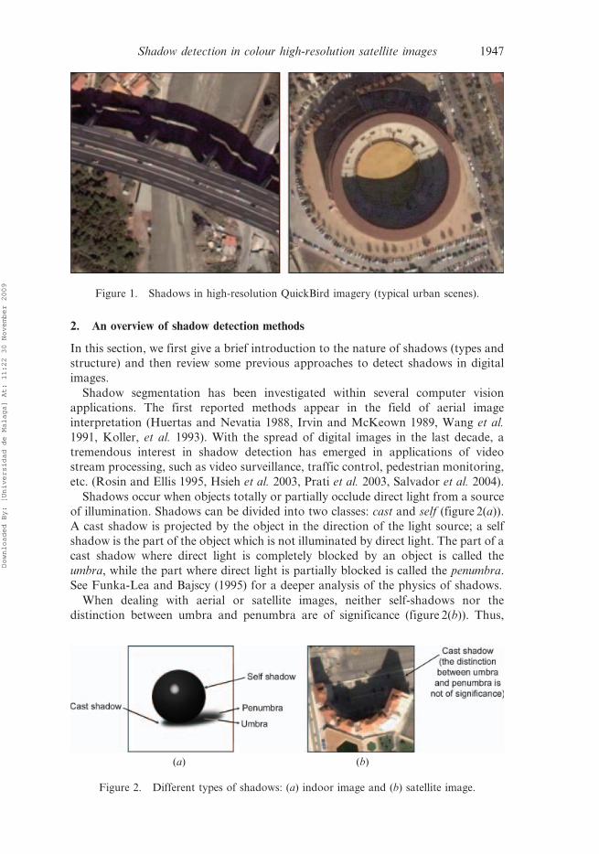
The improvement in spatial resolution of satellite imagery also implies that
something inherent to images, such as shadows, take on special significance for
different reasons (figure 1). On the one hand, they cause the partial or total loss of
radiometric information in the affected areas, and consequently they make image-
analysis processes like object detection and recognition, temporal change detection,
3D scene reconstruction, etc. more difficult or even fail. On the other hand, we may
take advantage of the presence of shadows as a valuable cue for inferring 3D scene
information based on the position and shape of the cast shadow, for example, for
building detection, delineation, and height estimation (Irvin and McKeown 1989). It
is clear, then, the convenience of accurately detecting shadowed areas in satellite
images either to radiometrically correct them and/or to infer 3D information.
*Corresponding author. Email: [email protected]
International Journal of Remote Sensing
Vol. 29, No. 7, 10 April 2008, 1945–1963
International Journal of Remote SensingISSN 0143-1161 print/ISSN 1366-5901 online # 2008 Taylor & Francis
http://www.tandf.co.uk/journalsDOI: 10.1080/01431160701395302
Downloaded By: [Universidad de Malaga] At: 11:22 30 November 2009
Shadow detection has received considerable attention within the computer vision
field, though not much work has been done towards the application of these results
to high-resolution satellite images recently available. This paper describes the main
approaches to detect shadows in images, and analyses their suitability for being
applied to colour satellite imagery. Based on this study, we propose a procedure that
exploits invariant colour space as well as edge information to effectively and
accurately detect shadows, in particular for QuickBird images (0.6 m per pixel).
Additional information such as sun azimuth or object heights (DEM) is not
considered here.
Very briefly, the proposed method deals with shadow detection through a region
growing procedure which basically consists of two stages:
1. Small groups of pixels which are likely to be shadow are selected as seeds of
shadow regions. They are obtained from a neighbourhood of local maxima in
the c3 component of the c1c2c3 colour space. Each shadow area is then
characterized by a Gaussian distribution of the c3 values of the pixels within
this region. The c1c2c3 space, first proposed by Gevers and Smeulders (1999)
for colour-based object recognition, is computed from the RGB representation
through the following nonlinear transformations:
c1~arctanR
max G, Bf g
� �ð1Þ
c2~arctanG
max R, Bf g
� �ð2Þ
c3~arctanB
max R,Gf g
� �: ð3Þ
2. From these seeds, the shape of the shadow region is recursively extended by
adding adjacent pixels which are consistent with the above distribution. To
delimit as precisely as possible the shape of the shadowed area, this process
takes into account region boundary information provided by an edge
detector.
One of the problems when using the c3 component is its instability for certain
colour values that leads to the misclassification of non-shadow pixels as shadow
(false positives). As reported in Gevers and Smeulders (1999) and Salvador et al.
(2004), this occurs both for pixels with low values of saturation and for pixels with
extreme intensity values (either low or high). During the above two stages, to
overcome this problem some components of the HSV space are checked. The overall
approach has been successfully tested with QuickBird images acquired under
different lighting conditions taken in diverse seasons, with different sun elevation
angles and covering both urban and rural areas.
The remainder of this paper is organized as follows. In §2, we review some of the
most representative methods of detecting shadows in digital images. In §3, we
describe some colour spaces of special interest for shadow detection. In §4, the
proposed method is described. In §5, we present experimental results. Finally, some
conclusions and future work are outlined.
1946 V. Arevalo et al.
Downloaded By: [Universidad de Malaga] At: 11:22 30 November 2009
2. An overview of shadow detection methods
In this section, we first give a brief introduction to the nature of shadows (types and
structure) and then review some previous approaches to detect shadows in digital
images.
Shadow segmentation has been investigated within several computer vision
applications. The first reported methods appear in the field of aerial image
interpretation (Huertas and Nevatia 1988, Irvin and McKeown 1989, Wang et al.
1991, Koller, et al. 1993). With the spread of digital images in the last decade, a
tremendous interest in shadow detection has emerged in applications of video
stream processing, such as video surveillance, traffic control, pedestrian monitoring,
etc. (Rosin and Ellis 1995, Hsieh et al. 2003, Prati et al. 2003, Salvador et al. 2004).
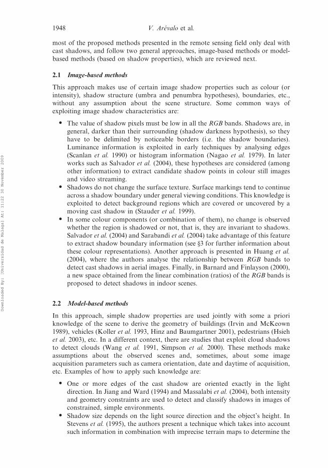
Shadows occur when objects totally or partially occlude direct light from a source
of illumination. Shadows can be divided into two classes: cast and self (figure 2(a)).
A cast shadow is projected by the object in the direction of the light source; a self
shadow is the part of the object which is not illuminated by direct light. The part of a
cast shadow where direct light is completely blocked by an object is called the
umbra, while the part where direct light is partially blocked is called the penumbra.
See Funka-Lea and Bajscy (1995) for a deeper analysis of the physics of shadows.
When dealing with aerial or satellite images, neither self-shadows nor the
distinction between umbra and penumbra are of significance (figure 2(b)). Thus,
(a) (b)
Figure 2. Different types of shadows: (a) indoor image and (b) satellite image.
Figure 1. Shadows in high-resolution QuickBird imagery (typical urban scenes).
Shadow detection in colour high-resolution satellite images 1947
Downloaded By: [Universidad de Malaga] At: 11:22 30 November 2009
most of the proposed methods presented in the remote sensing field only deal with
cast shadows, and follow two general approaches, image-based methods or model-
based methods (based on shadow properties), which are reviewed next.
2.1 Image-based methods
This approach makes use of certain image shadow properties such as colour (or
intensity), shadow structure (umbra and penumbra hypotheses), boundaries, etc.,
without any assumption about the scene structure. Some common ways of
exploiting image shadow characteristics are:
N The value of shadow pixels must be low in all the RGB bands. Shadows are, in
general, darker than their surrounding (shadow darkness hypothesis), so they
have to be delimited by noticeable borders (i.e. the shadow boundaries).
Luminance information is exploited in early techniques by analysing edges
(Scanlan et al. 1990) or histogram information (Nagao et al. 1979). In later
works such as Salvador et al. (2004), these hypotheses are considered (among
other information) to extract candidate shadow points in colour still images
and video streaming.
N Shadows do not change the surface texture. Surface markings tend to continue
across a shadow boundary under general viewing conditions. This knowledge is
exploited to detect background regions which are covered or uncovered by a
moving cast shadow in (Stauder et al. 1999).
N In some colour components (or combination of them), no change is observed
whether the region is shadowed or not, that is, they are invariant to shadows.
Salvador et al. (2004) and Sarabandi et al. (2004) take advantage of this feature
to extract shadow boundary information (see §3 for further information about
these colour representations). Another approach is presented in Huang et al.
(2004), where the authors analyse the relationship between RGB bands to
detect cast shadows in aerial images. Finally, in Barnard and Finlayson (2000),
a new space obtained from the linear combination (ratios) of the RGB bands is
proposed to detect shadows in indoor scenes.
2.2 Model-based methods
In this approach, simple shadow properties are used jointly with some a priori
knowledge of the scene to derive the geometry of buildings (Irvin and McKeown
1989), vehicles (Koller et al. 1993, Hinz and Baumgartner 2001), pedestrians (Hsieh
et al. 2003), etc. In a different context, there are studies that exploit cloud shadows
to detect clouds (Wang et al. 1991, Simpson et al. 2000). These methods make
assumptions about the observed scenes and, sometimes, about some image
acquisition parameters such as camera orientation, date and daytime of acquisition,
etc. Examples of how to apply such knowledge are:
N One or more edges of the cast shadow are oriented exactly in the light
direction. In Jiang and Ward (1994) and Massalabi et al. (2004), both intensity
and geometry constraints are used to detect and classify shadows in images of
constrained, simple environments.
N Shadow size depends on the light source direction and the object’s height. In
Stevens et al. (1995), the authors present a technique which takes into account
such information in combination with imprecise terrain maps to determine the
1948 V. Arevalo et al.
Downloaded By: [Universidad de Malaga] At: 11:22 30 November 2009
probability that a given point in an aerial photographs is either in sunlight or in
shadow.
In general, the shadow detection techniques proposed in these works are quite
simplified processes (typically, thresholding) which are usually part of a more
complex system that refines the shadow area (along with the model of the object that
has cast it) through a hypothesis-verification framework. In some works, the
accuracy in confining the shadow region is not important, since it is only employed
as a cue for the presence of buildings (typically, detecting shadows is easier than
detecting buildings, pedestrians, cars, etc.).The main limitation of these methods is
that they are designed for specific applications and for a particular type of object.
Therefore, in complex scenes, as is usually the case for high-resolution images, they
are not general enough for coping with the great diversity of geometric structures
they may contain.
Our technique for shadow detection is a pure image-based method, since we
exclusively apply image properties. In particular, we exploit both a shadow invariant
colour component and edge information. Although the Sun azimuth and sensor/
camera localization are typically available for satellite images (i.e. in QuickBird), we
do not make use of this information since, in general, it is not possible to derive
precise model of the acquired area (in most cases, the 3D geometry of scene is
unknown or of a great complexity).
Next, we analyse the c3 component of the c1c2c3 colour space and its suitability for
being applied to shadow detection in colour high-resolution satellite images.
3. c3 colour component
Colour can be represented in a variety of three dimensional spaces, such as RGB,
HSV, XYZ, c1c2c3, l1l2l3, YCrCb, Lab, Luv, etc. (Ford and Roberts 1998). Each
colour space is characterized by interesting properties which make it especially
appropriate for a specific application. Among these properties, we can highlight the
invariant features. For example, some colour spaces are invariant to changes in the
imaging conditions including viewing direction, object surface orientation, lighting
conditions, and shadows. Traditional colour spaces such as normalized-RGB (rgb),
hue and saturation (from HSV), and, more recently, c1c2c3 (Gevers and Smeulders
1999) are colour representations that have revealed some kind of shadow invariant
property. Of remarkable effectiveness is the latter, c1c2c3, which has been
successfully used by Salvador et al. (2004) to extract shadows in simple images
with few single-colour objects and a flat (non-textured) background. Obviously,
these premises cannot be assumed in high-resolution colour satellite images where
the observed scenes are highly textured, objects may have many different colours,
and the scene, in general, is very complex (figure 3). In Sarabandi et al. (2004), the
authors also employ this representation to extract shadow boundaries in high-
resolution images by means of a texture filter.
To evaluate the limitations of the c1c2c3 space for shadow detection, we have
performed tests over a broad set of QuickBird images, acquired under different
lighting conditions and covering both urban and rural areas. The results of our
tests verifies the suitability of the c3 component to identify shadowed regions
which produce a much higher response than those non-shadowed (figure 3).
Despite these promising possibilities, our tests have also revealed the following
problems:
Shadow detection in colour high-resolution satellite images 1949
Downloaded By: [Universidad de Malaga] At: 11:22 30 November 2009

N The c3 band is quite noisy, which causes the misclassification of shadow pixels
as non-shadow (true negatives) as well as inaccuracies in the shadow
boundaries.
N Equation (3) becomes unstable for low saturation (S) values (i.e. grey levels),
which causes the misclassification of non-shadow pixels as shadow (false
positives) (e.g. asphalt, concrete areas, etc.). This behaviour has also been
reported by Gevers and Smeulders (1999).
N Colours close to blue (high values of B) are wrongly detected as shadows (false
positives). In our test images, typically this occurs for blue water (i.e. swimming
pools), as illustrated in figure 3.
To overcome the above problems, in our approach we incorporate the following
two actuations:
Figure 3. Typical urban scenes that illustrate the complexity of high-resolution coloursatellite images (e.g. highly textured, objects may have many different colours, etc.) and theircorresponding c3 components. Local maxima produced by saturated white areas (bottom left)and swimming pools (bottom right) are marked in both images.
1950 V. Arevalo et al.
Downloaded By: [Universidad de Malaga] At: 11:22 30 November 2009
N To minimize the noise effect, the c3 image is smoothed, and we make use of the
intensity image gradient to define more precisely the shadow areas.
N We check the components S and V (from HSV) and do not classify a pixel as
shadow if it is one of the above cases. This may give rise to small gaps in a
shadow region, but it is a minor cost to pay for avoiding false positives,
especially since these small gaps may be filled later by a morphological filter.
Next, we describe the developed method, which is based on the segmentation of a
smoothed c3 image while taking into account the aforementioned considerations.
4. Description of the proposed method
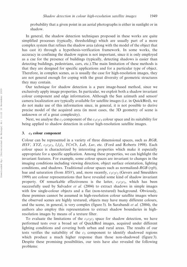
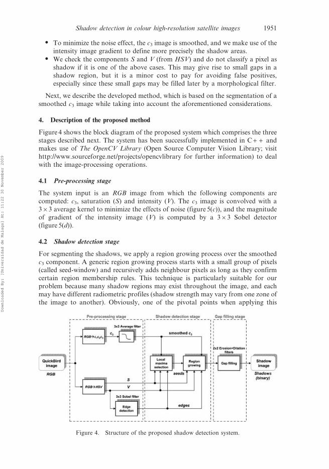
Figure 4 shows the block diagram of the proposed system which comprises the three
stages described next. The system has been successfully implemented in C + + and
makes use of The OpenCV Library (Open Source Computer Vision Library; visit
http://www.sourceforge.net/projects/opencvlibrary for further information) to deal
with the image-processing operations.
4.1 Pre-processing stage
The system input is an RGB image from which the following components are
computed: c3, saturation (S) and intensity (V). The c3 image is convolved with a
363 average kernel to minimize the effects of noise (figure 5(c)), and the magnitude
of gradient of the intensity image (V) is computed by a 363 Sobel detector
(figure 5(d)).
4.2 Shadow detection stage
For segmenting the shadows, we apply a region growing process over the smoothed
c3 component. A generic region growing process starts with a small group of pixels
(called seed-window) and recursively adds neighbour pixels as long as they confirm
certain region membership rules. This technique is particularly suitable for our
problem because many shadow regions may exist throughout the image, and each
may have different radiometric profiles (shadow strength may vary from one zone of
the image to another). Obviously, one of the pivotal points when applying this
Figure 4. Structure of the proposed shadow detection system.
Shadow detection in colour high-resolution satellite images 1951
Downloaded By: [Universidad de Malaga] At: 11:22 30 November 2009
technique is that of reliably placing the seeds in the image: at least one per shadow
region (irrespective if they are redundant) and no seed at non-shadow pixels. Next,
we describe our implementation of this technique in more depth.
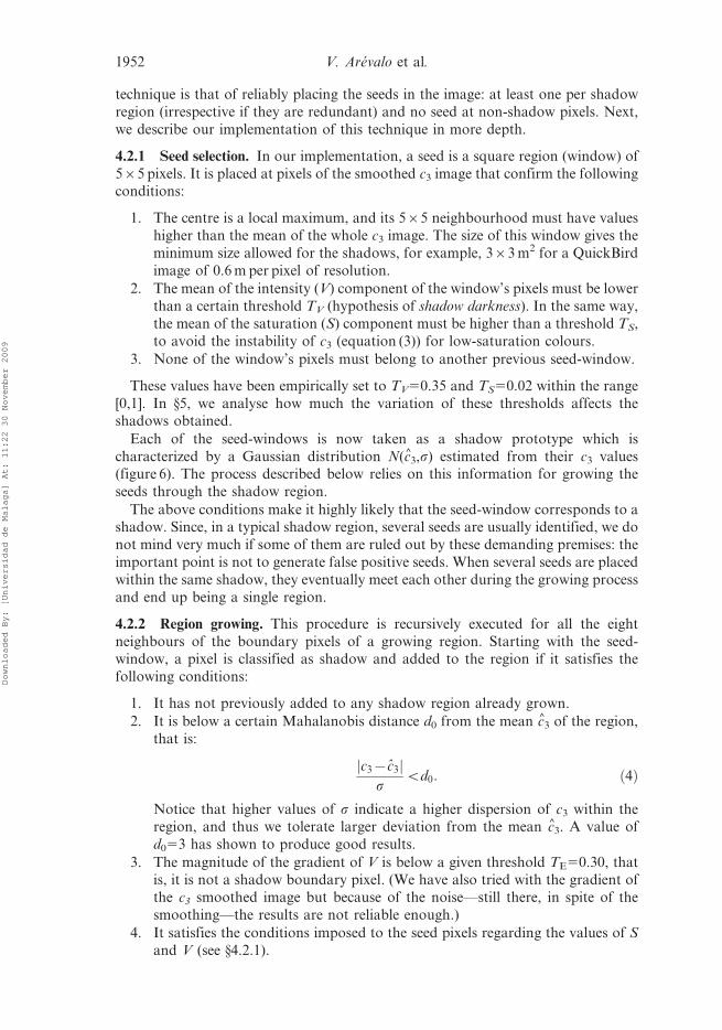
4.2.1 Seed selection. In our implementation, a seed is a square region (window) of
565 pixels. It is placed at pixels of the smoothed c3 image that confirm the followingconditions:
1. The centre is a local maximum, and its 565 neighbourhood must have values
higher than the mean of the whole c3 image. The size of this window gives the
minimum size allowed for the shadows, for example, 363 m2 for a QuickBird
image of 0.6 m per pixel of resolution.
2. The mean of the intensity (V) component of the window’s pixels must be lower
than a certain threshold TV (hypothesis of shadow darkness). In the same way,
the mean of the saturation (S) component must be higher than a threshold TS,
to avoid the instability of c3 (equation (3)) for low-saturation colours.
3. None of the window’s pixels must belong to another previous seed-window.
These values have been empirically set to TV50.35 and TS50.02 within the range
[0,1]. In §5, we analyse how much the variation of these thresholds affects theshadows obtained.
Each of the seed-windows is now taken as a shadow prototype which is
characterized by a Gaussian distribution N(c^3,s) estimated from their c3 values(figure 6). The process described below relies on this information for growing the
seeds through the shadow region.
The above conditions make it highly likely that the seed-window corresponds to ashadow. Since, in a typical shadow region, several seeds are usually identified, we do
not mind very much if some of them are ruled out by these demanding premises: the
important point is not to generate false positive seeds. When several seeds are placed
within the same shadow, they eventually meet each other during the growing process
and end up being a single region.
4.2.2 Region growing. This procedure is recursively executed for all the eight
neighbours of the boundary pixels of a growing region. Starting with the seed-window, a pixel is classified as shadow and added to the region if it satisfies the
following conditions:
1. It has not previously added to any shadow region already grown.
2. It is below a certain Mahalanobis distance d0 from the mean c^3 of the region,
that is:
c3{c3j js
vd0: ð4Þ
Notice that higher values of s indicate a higher dispersion of c3 within theregion, and thus we tolerate larger deviation from the mean c^3. A value of
d053 has shown to produce good results.
3. The magnitude of the gradient of V is below a given threshold TE50.30, thatis, it is not a shadow boundary pixel. (We have also tried with the gradient of
the c3 smoothed image but because of the noise—still there, in spite of the
smoothing—the results are not reliable enough.)
4. It satisfies the conditions imposed to the seed pixels regarding the values of S
and V (see §4.2.1).
1952 V. Arevalo et al.
Downloaded By: [Universidad de Malaga] At: 11:22 30 November 2009

If the pixel is incorporated into the region, the Gaussian distribution N(c^3,s) is
updated with its c3 value. The process ends when none of the neighbour pixels has
been added to the region.
Notice that, during the growing process of a particular seed, pixels of different
seed-windows not processed yet can be evaluated as any other image pixel. If their
inclusion in the region is accepted, that seed is removed from the list of remaining
seeds to be grown. We have checked that there is not much difference in the results
between this sequential implementation and a concurrent one since, in the end, all of
the obtained regions are going to be merged into a single indistinctive one after the
gap filling stage (to be described next).
(a) (b)
Figure 6. (a) Shadow seeds identified in the smoothed c3 component. (b) A shadow seedwindow.
(a)
(b) (c) (d )
Figure 5. (a) Colour components computed from the RGB image. (b) Horizontal scan lineswhich illustrate the effects of smoothing stage in the c3 component. The images (c) and (d)show the results of the image processes described in section 3, that is, the smoothed c3
component and the module of gradient of V, respectively.
Shadow detection in colour high-resolution satellite images 1953
Downloaded By: [Universidad de Malaga] At: 11:22 30 November 2009
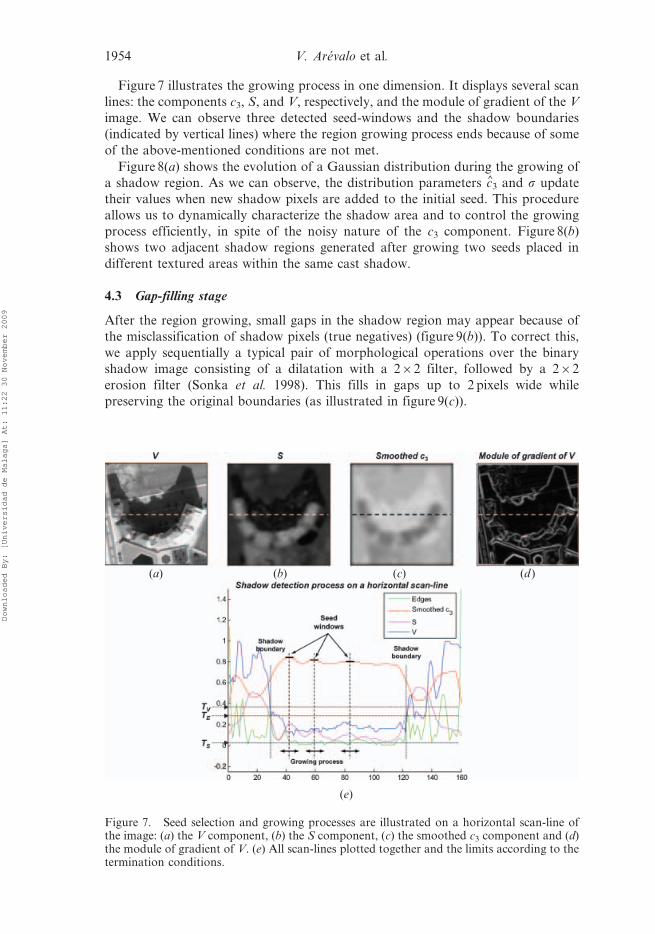
Figure 7 illustrates the growing process in one dimension. It displays several scan
lines: the components c3, S, and V, respectively, and the module of gradient of the V
image. We can observe three detected seed-windows and the shadow boundaries
(indicated by vertical lines) where the region growing process ends because of some
of the above-mentioned conditions are not met.
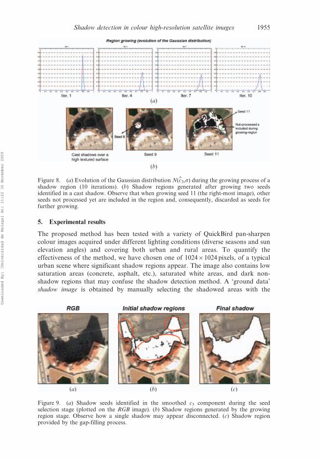
Figure 8(a) shows the evolution of a Gaussian distribution during the growing of
a shadow region. As we can observe, the distribution parameters c^3 and s update
their values when new shadow pixels are added to the initial seed. This procedure
allows us to dynamically characterize the shadow area and to control the growing
process efficiently, in spite of the noisy nature of the c3 component. Figure 8(b)
shows two adjacent shadow regions generated after growing two seeds placed in
different textured areas within the same cast shadow.
4.3 Gap-filling stage
After the region growing, small gaps in the shadow region may appear because of
the misclassification of shadow pixels (true negatives) (figure 9(b)). To correct this,
we apply sequentially a typical pair of morphological operations over the binary
shadow image consisting of a dilatation with a 262 filter, followed by a 262
erosion filter (Sonka et al. 1998). This fills in gaps up to 2 pixels wide while
preserving the original boundaries (as illustrated in figure 9(c)).
(a) (b)
(e)
(c) (d )
Figure 7. Seed selection and growing processes are illustrated on a horizontal scan-line ofthe image: (a) the V component, (b) the S component, (c) the smoothed c3 component and (d)the module of gradient of V. (e) All scan-lines plotted together and the limits according to thetermination conditions.
1954 V. Arevalo et al.
Downloaded By: [Universidad de Malaga] At: 11:22 30 November 2009
5. Experimental results
The proposed method has been tested with a variety of QuickBird pan-sharpen
colour images acquired under different lighting conditions (diverse seasons and sun
elevation angles) and covering both urban and rural areas. To quantify the
effectiveness of the method, we have chosen one of 102461024 pixels, of a typical
urban scene where significant shadow regions appear. The image also contains low
saturation areas (concrete, asphalt, etc.), saturated white areas, and dark non-
shadow regions that may confuse the shadow detection method. A ‘ground data’
shadow image is obtained by manually selecting the shadowed areas with the
(a) (b) (c)
Figure 9. (a) Shadow seeds identified in the smoothed c3 component during the seedselection stage (plotted on the RGB image). (b) Shadow regions generated by the growingregion stage. Observe how a single shadow may appear disconnected. (c) Shadow regionprovided by the gap-filling process.
(a)
(b)
Figure 8. (a) Evolution of the Gaussian distribution N(c^3,s) during the growing process of ashadow region (10 iterations). (b) Shadow regions generated after growing two seedsidentified in a cast shadow. Observe that when growing seed 11 (the right-most image), otherseeds not processed yet are included in the region and, consequently, discarded as seeds forfurther growing.
Shadow detection in colour high-resolution satellite images 1955
Downloaded By: [Universidad de Malaga] At: 11:22 30 November 2009
selection tools included in a well-known image-processing package (AdobeHPhotoshopH). Through a pixel-by-pixel comparison with this shadow image we
have classified the pixels of our test images as true/false positive/negative (TP, TN,
FP, and FN). A pixel is set to be TP/FP if it is correctly/erroneously detected as
shadow, and TN/FN when it is correctly/erroneously detected as non-shadow. Both
true positives (TP) and true negatives (TN) are correct classifications, while the
others are misclassifications.
Three statistics that capture the goodness of these four values are: the Producer’s
Accuracy (PA), also called sensitivity (Kanji 1999), the Consumer’s Accuracy (CA),
and the Overall Accuracy (OA), which are defined as follows:
PA ~TP
TPzFN|100 ð5Þ
CA~TP
TPzFP|100 ð6Þ
OA~TPzTN
TPzFPzTNzFN|100: ð7Þ
For completeness, we also include the specificity (SP) (Kanji 1999), which is
defined as:
SP~TN
TNzFP|100: ð8Þ
Notice that TP + FN and TN + FP are the shadow and non-shadow ground data,
respectively. Consequently, the producer’s accuracy indicates the probability of the
method of correctly classifying a pixel as shadow among those which are actually
shadow, while the specificity gives us the probability of the method of correctly
classifying a pixel as non-shadow among those which are actually non-shadow.
Thus, the greater these two statistics, the better the detection process.
Since our method makes use of information from edges and different colour
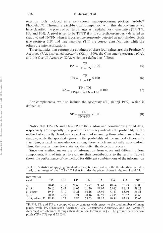
components, it is of interest to evaluate their contributions to the results. Table 1
shows the performance of the method for different combinations of the information
Table 1. Statistics of applying our shadow detection method with the thresholds reported in§4, to an image of size 102461024 that includes the pieces shown in figures 11 and 13.
Informationused TP FN FP TN PA CA OA SP
c3 20.46 2.17 21.60 55.77 90.41 48.64 76.23 72.08c3, S 20.15 2.47 16.07 61.30 89.07 55.65 81.45 79.23c3, edges 19.44 3.19 11.21 66.16 85.92 63.43 85.60 85.51c3, V 20.36 2.27 7.21 70.16 89.98 73.85 90.52 90.68c3, S, edges, V 18.36 4.27 1.85 75.53 81.15 90.94 93.89 97.62
TP, FN, FP, and TN are computed as percentages with respect to the total number of imagepixels, while PA (Producer’s Accuracy), CA (Consumer’s Accuracy), and OA (Overall’sAccuracy) are obtained through their definition formulas in §5. The ground data shadowpixels (TP + FN) equal 22.63%.
1956 V. Arevalo et al.
Downloaded By: [Universidad de Malaga] At: 11:22 30 November 2009
managed by the region growing procedure. For example, <c3,V> refers to the
application of the region growing without taking into account the restrictions
regarding the gradient of V (edges) and saturation. This table reveals the importance
of including, apart from the c3 component, the three additional constraints (for S, V
and gradient values). Among these three constraints, it is remarkable the effect of
the hypothesis of darkness of shadows (the V value below a threshold TV), which
produces an important decrease in the percentage of FP. In this implementation, the
thresholds for the set of constraints (c3, S, Edges, V ) have been selected to be very
restrictive in not detecting non-shadow pixels as shadow (high consumer accuracy),
at the cost of missing some true shadows (producer’s accuracy); observe in the last
row of table 1 that the percentage of TP falls slightly.
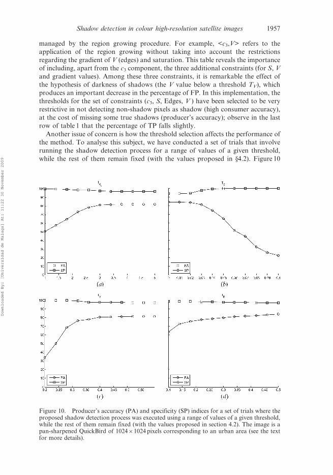
Another issue of concern is how the threshold selection affects the performance of
the method. To analyse this subject, we have conducted a set of trials that involve
running the shadow detection process for a range of values of a given threshold,
while the rest of them remain fixed (with the values proposed in §4.2). Figure 10
Figure 10. Producer’s accuracy (PA) and specificity (SP) indices for a set of trials where theproposed shadow detection process was executed using a range of values of a given threshold,while the rest of them remain fixed (with the values proposed in section 4.2). The image is apan-sharpened QuickBird of 102461024 pixels corresponding to an urban area (see the textfor more details).
Shadow detection in colour high-resolution satellite images 1957
Downloaded By: [Universidad de Malaga] At: 11:22 30 November 2009
shows the results of these experiments in terms of the producer’s accuracy and
specificity indices, where the following points can be highlighted:
1. The specificity is always high regardless of the threshold value (for all the
plots), because the TP remains small in comparison with the TN (its slight
drop may be due to a significant increase in the FP). Notice that, when the
specificity decreases, the producer’s accuracy increases, so we must select the
threshold to balance between these two opposite behaviours: good in detecting
shadows or in not detecting non-shadows.
2. With the exception of the edge threshold (TE), all the plots present ‘flat’
intervals where the threshold values can vary without affecting the PA of the
output of the procedure too much. For example, any value of TS can be
selected within the range [0.01–0.03] giving almost the same result. This is
important, because it allows us certain tolerance in the selection of these
parameters.
3. From our tests with other different images (not shown here) we have verified
that optimal threshold values may slightly change with their brightness,
contrast, colour balance, etc. However, it has also been checked that
intermediate thresholds in the middle of these intervals produce satisfactory
(though not optimal) results for a wide variety of images.
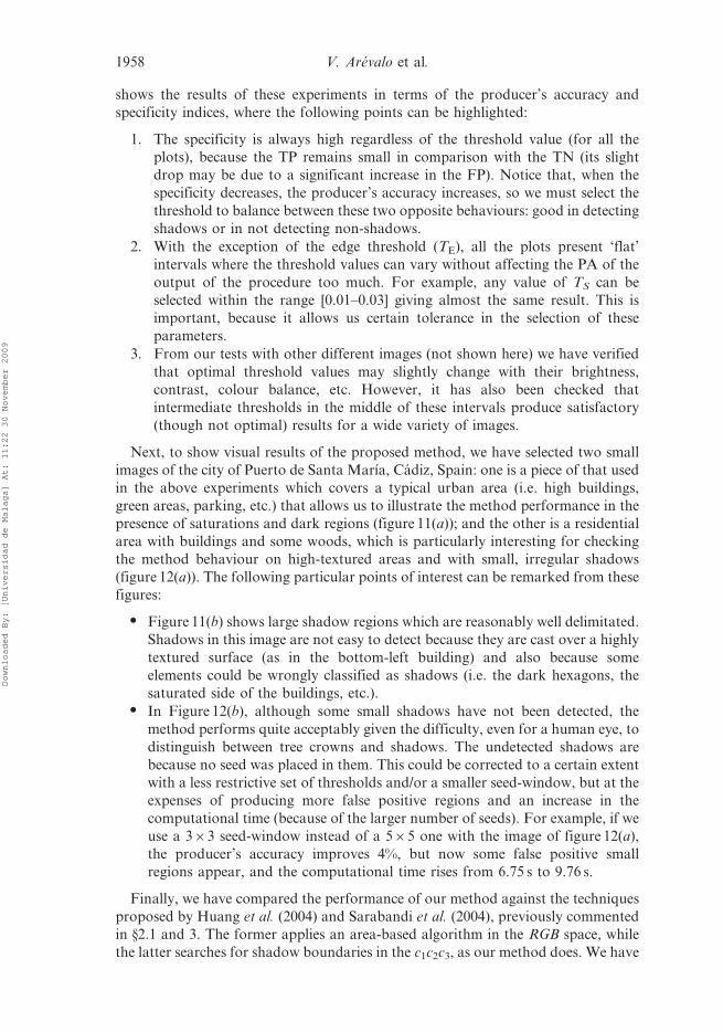
Next, to show visual results of the proposed method, we have selected two small
images of the city of Puerto de Santa Marıa, Cadiz, Spain: one is a piece of that used
in the above experiments which covers a typical urban area (i.e. high buildings,
green areas, parking, etc.) that allows us to illustrate the method performance in the
presence of saturations and dark regions (figure 11(a)); and the other is a residential
area with buildings and some woods, which is particularly interesting for checking
the method behaviour on high-textured areas and with small, irregular shadows
(figure 12(a)). The following particular points of interest can be remarked from these
figures:
N Figure 11(b) shows large shadow regions which are reasonably well delimitated.
Shadows in this image are not easy to detect because they are cast over a highly
textured surface (as in the bottom-left building) and also because some
elements could be wrongly classified as shadows (i.e. the dark hexagons, the
saturated side of the buildings, etc.).
N In Figure 12(b), although some small shadows have not been detected, the
method performs quite acceptably given the difficulty, even for a human eye, to
distinguish between tree crowns and shadows. The undetected shadows are
because no seed was placed in them. This could be corrected to a certain extent
with a less restrictive set of thresholds and/or a smaller seed-window, but at the
expenses of producing more false positive regions and an increase in the
computational time (because of the larger number of seeds). For example, if we
use a 363 seed-window instead of a 565 one with the image of figure 12(a),
the producer’s accuracy improves 4%, but now some false positive small
regions appear, and the computational time rises from 6.75 s to 9.76 s.
Finally, we have compared the performance of our method against the techniques
proposed by Huang et al. (2004) and Sarabandi et al. (2004), previously commented
in §2.1 and 3. The former applies an area-based algorithm in the RGB space, while
the latter searches for shadow boundaries in the c1c2c3, as our method does. We have
1958 V. Arevalo et al.
Downloaded By: [Universidad de Malaga] At: 11:22 30 November 2009
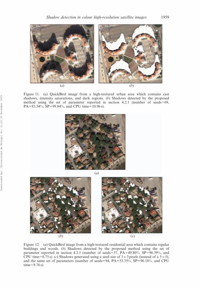
(a)
(b) (c)
Figure 12. (a) QuickBird image from a high-textured residential area which contains regularbuildings and woods. (b) Shadows detected by the proposed method using the set ofparameter reported in section 4.2.1 (number of seeds557, PA549.80%, SP596.39%, andCPU time56.75 s). (c) Shadows generated using a seed size of 363 pixels (instead of a 565),and the same set of parameters (number of seeds594, PA553.35%, SP596.18%, and CPUtime59.76 s).
(a) (b)
Figure 11. (a) QuickBird image from a high-textured urban area which contains castshadows, intensity saturations, and dark regions. (b) Shadows detected by the proposedmethod using the set of parameter reported in section 4.2.1 (number of seeds569,PA583.54%, SP599.84%, and CPU time510.96 s).
Shadow detection in colour high-resolution satellite images 1959
Downloaded By: [Universidad de Malaga] At: 11:22 30 November 2009
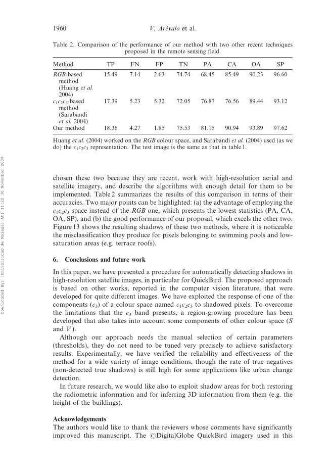
chosen these two because they are recent, work with high-resolution aerial and
satellite imagery, and describe the algorithms with enough detail for them to be
implemented. Table 2 summarizes the results of this comparison in terms of their
accuracies. Two major points can be highlighted: (a) the advantage of employing the
c1c2c3 space instead of the RGB one, which presents the lowest statistics (PA, CA,
OA, SP), and (b) the good performance of our proposal, which excels the other two.
Figure 13 shows the resulting shadows of these two methods, where it is noticeable
the misclassification they produce for pixels belonging to swimming pools and low-
saturation areas (e.g. terrace roofs).
6. Conclusions and future work
In this paper, we have presented a procedure for automatically detecting shadows in
high-resolution satellite images, in particular for QuickBird. The proposed approach
is based on other works, reported in the computer vision literature, that were
developed for quite different images. We have exploited the response of one of the
components (c3) of a colour space named c1c2c3 to shadowed pixels. To overcome
the limitations that the c3 band presents, a region-growing procedure has been
developed that also takes into account some components of other colour space (S
and V ).
Although our approach needs the manual selection of certain parameters
(thresholds), they do not need to be tuned very precisely to achieve satisfactory
results. Experimentally, we have verified the reliability and effectiveness of the
method for a wide variety of image conditions, though the rate of true negatives
(non-detected true shadows) is still high for some applications like urban change
detection.
In future research, we would like also to exploit shadow areas for both restoring
the radiometric information and for inferring 3D information from them (e.g. the
height of the buildings).
Acknowledgements
The authors would like to thank the reviewers whose comments have significantly
improved this manuscript. The #DigitalGlobe QuickBird imagery used in this
Table 2. Comparison of the performance of our method with two other recent techniquesproposed in the remote sensing field.
Method TP FN FP TN PA CA OA SP
RGB-basedmethod(Huang et al.2004)
15.49 7.14 2.63 74.74 68.45 85.49 90.23 96.60
c1c2c3-basedmethod(Sarabandiet al. 2004)
17.39 5.23 5.32 72.05 76.87 76.56 89.44 93.12
Our method 18.36 4.27 1.85 75.53 81.15 90.94 93.89 97.62
Huang et al. (2004) worked on the RGB colour space, and Sarabandi et al. (2004) used (as wedo) the c1c2c3 representation. The test image is the same as that in table 1.
1960 V. Arevalo et al.
Downloaded By: [Universidad de Malaga] At: 11:22 30 November 2009

study is distributed by Eurimage, SpA (www.eurimage.com) and provided by
Decasat Ingenieria S.L., Malaga, Spain (www.decasat.com).
ReferencesADAMS, B.J., WABNITZ, C., GHOSH, S., ALDER, J., CHUENPAGDEE, R., CHANG, S.E., BERKE, P.R.
and REES, W.E., 2005, Application of Landsat 5 and high-resolution optical satellite
imagery to investigate urban tsunami damage. In III International Workshop on Remote
Sensing for Post-Disaster Response, 12–13 September, Chiba, Japan.
BARNARD, K. and FINLAYSON, G., 2000, Shadow identification using color ratios. In IS&T/
SID VIII Color Imaging Conference: Color Science, Systems and Applications, pp.
97–101.
DEL-FRATE, F., SCHIAVON, G. and SOLIMINI, C., 2005, Change detection in urban areas with
QuickBird imagery and neural networks algorithms. In III ISPRS International
Symposium Remote Sensing and Data Fusion Over Urban Areas (URBAN’05), 14–16
March, Tempe, AZ.
FORD, A. and ROBERTS, A., 1998, Colour space conversions. Technical report, Westminster
University, London.
FUNKA-LEA, G. and BAJSCY, R., 1995, Combining colour and geometry for the active, visual
recognition of shadows. In V IEEE International Conference on Computer Vision
(ICCV’95), 20–23 June, Boston, MA, pp. 203–209.
GEVERS, T. and SMEULDERS, A.W.M., 1999, Colour-based object recognition. Pattern
Recognition, 32, pp. 453–464.
(a) (b) (c)
Figure 13. Comparison of the shadow areas detected by our algorithm (in (a)) and twoother methods: (b) using the RGB space (Huang et al., 2004) and (c) using the c1c2c3 space(Sarabandi et al., 2004). Observe the wrong classification in (b) and (c) of the swimming poolsas well as some low-saturated areas in the terrace roofs.
Shadow detection in colour high-resolution satellite images 1961
Downloaded By: [Universidad de Malaga] At: 11:22 30 November 2009
HINZ, S. and BAUMGARTNER, A., 2001, Vehicle detection in aerial images using
generic features, grouping, and context. In Pattern Recognition 2001 (DAGM
Symposium 2001), 2191 of Lecture Notes in Computer Science (Berlin: Springer), pp.
45–52.
HSIEH, J., HU, W., CHANG, C. and CHEN, Y., 2003, Shadow elimination for effective moving
object detection by gaussian shadow modeling. Journal of Image and Vision
Computing, 21, pp. 505–516.
HUANG, J., XIE, W. and TANG, L., 2004, Detection of and compensation for shadows in
coloured urban aerial images. In V IEEE World Congress on Intelligent Control and
Automation, 15–19 June, Hangzhou, P.R. China, pp. 3098–3100.
HUERTAS, A. and NEVATIA, R., 1988, Detecting buildings in aerial images. Computer Vision,
Graphics and Image Processing, 41, pp. 131–152.
IRVIN, B. and MCKEOWN, J.R., 1989, Methods for exploiting the relationship between
buildings and their shadows in aerial imagery. IEEE Transactions on System, Man and
Cybernetics, 19, pp. 1564–1575.
JIANG, C. and WARD, M.O., 1994, Shadow segmentation and classification in a constrained
environment. CVGIP: Image Understanding, 59, pp. 213–225.
KANJI, G.K., 1999, 100 Statistical Tests (Thousand Oaks, CA: SAGE).
KOLLER, D., DANIILIDIS, K. and NAGEL, H., 1993, Model-based object tracking in monocular
image sequences of road traffic scenes. International Journal of Computer Vision, 10,
pp. 257–281.
MASSALABI, A., HE, D.C., BENIE, G.B. and BEAUDRY, E., 2004, Restitution of information
under shadow in remote sensing high space resolution images: Application to
IKONOS data of Sherbrooke city. In XX ISPRS Congress, 12–23 July, Istanbul,
Turkey.
NAGAO, M., MATSUTYAMA, T. and IKEDA, Y., 1979, Region extraction and shape analysis
in aerial photographs. Computer Vision Graphics and Image Processing, 10, pp.
195–223.
PRATI, A., MIKIC, I., TRIVEDI, M.M. and CUCCHIARA, R., 2003, Detecting moving shadows:
algorithms and evaluation. IEEE Transactions on Pattern Analysis and Machine
Intelligence, 25, pp. 918–923.
ROSIN, P.L. and ELLIS, T., 1995, Image difference threshold strategies and shadow
detection. In 1995 British Conference on Machine Vision, July, Birmingham, UK, 1,
pp. 347–356.
SALVADOR, E., CAVALLARO, A. and EBRAHIMI, T., 2004, Cast shadow segmentation using
invariant colour features. Computer Vision and Image Understanding, 95, pp. 238–259.
SARABANDI, P., YAMAZAKI, F., MATSUOKA, M. and KIREMIDJIAN, A., 2004, Shadow
detection and radiometric restoration in satellite high resolution images. In IEEE
International Geoscience and Remote Sensing Symposium (IGARSS), 20–24
September, Anchorage, AL, 6, pp. 3744–3747.
SCANLAN, J.M., CHABRIES, D.M. and CHRISTIANSEN, R., 1990, A shadow detection and
removal algorithm for 2-D images. In IEEE International Conference on Acoustic,
Speech, and Signal Processing (ICASSP), 3–6 April, Albuquerque, NM, 4, pp.
2057–2060.
SIMPSON, J.J., JIN, Z. and STITT, J.R., 2000, Cloud shadow detection under arbitrary viewing
and illumination conditions. IEEE Transactions on Geoscience and Remote Sensing,
38, pp. 972–976.
SONKA, M., HLAVAC, V. and BOYLE, R., 1998, Image Processing, Analysis and Machine
Vision, 2nd ed., pp. 188–199 (London: International Thomson Computer Press).
STAUDER, J., MELCH, R. and OSTERMANN, J., 1999, Detection of moving cast shadows for
object segmentation. IEEE Transactions on Multimedia, 1, pp. 65–77.
STEVENS, M.R., PYEATT, L.D., HOULTON, D.J. and GOSS, M., 1995, Locating shadows in
aerial photographs using imprecise elevation data. Computer Science Technical Report
CS-95–105, Colorado State University.
1962 V. Arevalo et al.
Downloaded By: [Universidad de Malaga] At: 11:22 30 November 2009
VU, T.T., MATSUOKA, M. and YAMAZAK, F., 2004, Shadow analysis in assisting damage
detection due to earthquakes from QuickBird imagery. In XX ISPRS Congress, 12–23
July, Istanbul, Turkey, pp. 607–610.
WANG, C., HUANG, L. and ROSENFELD, A., 1991, Detecting clouds and cloud shadows on
aerial photographs. Pattern Recognition Letters, 12, pp. 55–64.
Shadow detection in colour high-resolution satellite images 1963
Downloaded By: [Universidad de Malaga] At: 11:22 30 November 2009