Data Min Knowl DiscDOI 10.1007/s10618-014-0354-1

Approximating the crowd

Seyda Ertekin · Cynthia Rudin · Haym Hirsh

Received: 17 February 2013 / Accepted: 13 May 2014© The Author(s) 2014

Abstract The problem of “approximating the crowd” is that of estimating the crowd’smajority opinion by querying only a subset of it. Algorithms that approximate thecrowd can intelligently stretch a limited budget for a crowdsourcing task. We presentan algorithm, “CrowdSense,” that works in an online fashion where items come oneat a time. CrowdSense dynamically samples subsets of the crowd based on an explo-ration/exploitation criterion. The algorithm produces a weighted combination of thesubset’s votes that approximates the crowd’s opinion. We then introduce two varia-tions of CrowdSense that make various distributional approximations to handle distinctcrowd characteristics. In particular, the first algorithm makes a statistical independenceapproximation of the labelers for large crowds, whereas the second algorithm finds alower bound on how often the current subcrowd agrees with the crowd’s majority vote.Our experiments on CrowdSense and several baselines demonstrate that we can reli-ably approximate the entire crowd’s vote by collecting opinions from a representativesubset of the crowd.

Responsible editor: Hendrik Blockeel, Kristian Kersting, Siegfried Nijssen, Filip Zelezny.

Electronic supplementary material The online version of this article(doi:10.1007/s10618-014-0354-1) contains supplementary material, which is available to authorized users.

S. Ertekin (B) · C. RudinMIT CSAIL, Sloan School of Management, and Center for Collective Intelligence,Massachusetts Institute of Technology, Cambridge, MA, USAe-mail: seyda@mit.edu

C. Rudine-mail: rudin@mit.edu

H. HirshDepartment of Computer Science and Information Science, Cornell University, Ithaca, NY, USAe-mail: hirsh@cs.cornell.edu

123

S. Ertekin et al.

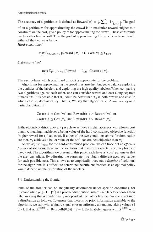
Keywords Crowdsourcing · Wisdom of crowds · Labeler quality estimation ·Approximating the crowd · Aggregating opinions

1 Introduction

Our goal is to determine the majority opinion of a crowd on a series of questions(“examples”), where each member’s opinion is obtained at a cost, and our total budgetis limited. For example, let us consider a sneaker company, wanting to do a customersurvey, where they provide free variants of a new sneaker to the members of a largecrowd of product testers, who each give a “yay” or “nay” to each product, one at atime. The company wants to know whether the majority of testers approves each newsneaker variant. Some product testers are more useful than others; some align closelywith the majority vote, and some do not. If the company can identify who are the mostuseful product testers, they can send new trial sneakers mostly to them, at a large costsavings.

This problem of estimating the majority vote on a budget goes well beyond producttesting—the problem occurs for many tasks falling under the umbrella of crowdsourc-ing, where the collective intelligence of large crowds is leveraged by combining theirinput on a set of examples. In crowdsourcing problems, either there is no ground truth(as the ultimate goal is to determine a judgment), or there is ground truth, but withno possibility of its being revealed. The application domain of answer services isrelevant to the problem of approximating the crowd. Here are some specific exampleapplications:

– VizWiz1 (Bigham et al. 2010) is an iPhone app used by visually impaired peopleto obtain answers to questions about their surroundings. VizWiz queries multi-ple Amazon Mechanical Turkers, and on its website, VizWiz issues the statement“VizWiz will recruit multiple answers from different web workers to help you bettergauge the reliability of answers retrieved in this way.” There may or may not beground truth in the questions posed on VizWiz, but either way, the majority voteof the crowd is likely to be the desired answer to the query. The more turkers youquery, the more confident you can be about the answer. However, if several turkersneed to be queried, it will take longer (with a cost) for the visually impaired personto retrieve the answer. If a system existed that could learn over time, as queriesproceed, who are the reliable members of the crowd that agree with its majorityvote, then the system could potentially be a valuable contributor to services likeVizWiz.

– IQ Engines2 is a crowdsourced image recognition platform. It uses a combinationof computer vision software and human labelers to identify objects in photographs.Over time, as it is queried more and more, it would be useful for the system to learnwho are the most reliable humans to answer the queries. This way, fewer humansneed to be involved over time, and only the most reliable humans need to be hired.

1 http://vizwiz.org2 http://iqengines.com/

123

Approximating the crowd

Again, there may or may not be ground truth, but the majority vote of the crowd islikely to be a desirable, or at least acceptable answer, by computer vision standards.

– Polling is by definition crowdsourced. In product design and manufacturing, com-panies have taken steps to interact with their customers and having them suggest,discuss and vote on new product ideas (Ogawa and Piller 2006; Sullivan 2010).They also commonly rely on focus groups and usability studies to collect the opin-ions of crowds on existing or new products. These companies would like, withminimal effort, cost, and speed, to estimate the crowd’s majority vote accurately. Inthe absence of sophisticated sampling techniques, collecting more votes per itemincreases the likelihood that the crowd’s opinion reflects the majority opinion ofthe entire population.In cases where each vote is provided at a cost, collecting avote from every member of the crowd in order to determine the majority opinioncan be expensive and may not be attainable under fixed budget constraints.

Because of the open nature of crowdsourcing systems, it is not necessarily easy toapproximate the majority vote of a crowd on a budget by sampling a representativesubset of the voters. For example, the crowd may be comprised of labelers with arange of capabilities, motives, knowledge, views, personalities, etc. Without any priorinformation about the characteristics of the labelers, a small sample of votes is notguaranteed to align with the true majority opinion. In order to effectively approximatethe crowd, we need to determine who are the most representative members of thecrowd, in that they can best represent the interests of the crowd majority. This is evenmore difficult to accomplish when items arrive over time as in the answer servicesapplications above, and it requires our budget to be used both for (1) estimating themajority vote, even before we understand the various qualities of each labeler, and (2)exploring the various labelers until we can estimate their qualities well. Estimating themajority vote in particular can be expensive before the labelers’ qualities are known,and we do not want to pay for additional votes that are not likely to impact the decision.

In order to make economical use of our budget, we could determine when justenough votes have been gathered to confidently align our decision with the crowdmajority. The budget limitation necessitates a compromise: if we pay for many votesper decision, our estimates will closely align with the crowd majority, but we will onlymake a smaller number of decisions, whereas if we pay for fewer votes per decision,the accuracy may suffer, but more decisions are made. There is clearly an explo-ration/exploitation tradeoff: before we can exploit by using mainly the best labelers,we need to explore to determine who these labelers are, based on their agreement withthe crowd.

The main contributions of this work can be broken down into three parts: In the firstpart (Sect. 3), we introduce the problem of approximating the crowd, and the notionof the frontier of cost and accuracy. We solve analytically for the expected values ofthe extreme points on the frontier.

In the second part of the paper (Sect. 4), we propose a modular algorithm, Crowd-Sense, that approximates the wisdom of the crowd. In an online fashion, CrowdSensedynamically samples a subset of labelers, determines whether it has enough votes tomake a decision, and requests more if the decision is sufficiently uncertain. Crowd-Sense keeps a balance between exploration and exploitation in its online iterations:

123

S. Ertekin et al.

exploitation in terms of seeking labels from the highest-rated labelers, and explo-ration so that enough data are obtained about each labeler to ensure that we learn eachlabeler’s accuracy sufficiently well. We present experiments across several datasetsand in comparison with several baselines in Sect. 6, where the cost constraint para-meter was set over several different values, and variants were computed over 100 runsto ensure the quality of the solution. We then discuss the effects of CrowdSense’sparameters in Sect. 7, and the effects of the various subcomponents in Sect. 8.

The third part of the paper presents probabilistic variations of CrowdSense, inSect. 9. One of the main challenges to approximating the crowd has to do with thefact that the majority vote is taken as the ground truth (the truth we aim to predict).This means that there is a complicated relationship (a joint probability distribution)between the labelers’ accuracies with respect to the majority vote. In Sects. 9.1 and 9.2of the paper, we introduce two variations of CrowdSense, called CrowdSense.Ind andCrowdSense.Bin, that make specific distributional approximations to handle distinctcrowd characteristics. In particular, the first algorithm makes a statistical independenceapproximation of the probabilities for large crowds, whereas the second algorithm findsa lower bound on how often the current subcrowd agrees with the crowd majority vote,using the binomial distribution. For both CrowdSense.Ind and CrowdSense.Bin, eventhough explicit probabilistic approximations were made, the accuracy is comparableto (or lower than) CrowdSense itself. It is difficult to characterize the joint distributionfor the problem of approximating the crowd, due to the constraint that the majority voteis the true label. CrowdSense, with its easy-to-understand weighted majority votingscheme, seems to capture the essence of the problem, and yet has the best performancewithin the pool of algorithms we tried. Experiments comparing the three CrowdSensevariants are in Sect. 10.

In the supplementary file3, in Section A, we present a proposition for Crowd-Sense.Bin that states that the computed scores are non-negative. Section B presentsa “flipping” technique – a heuristic for taking the opposite vote of labelers that havelow quality estimates. In Section C, we discuss the possibility of learning the labelers’quality estimates using machine learning. Section D presents the runtime performanceof the algorithms. Section E presents the effect of gold standard data in initialization.

Throughout the paper, a “majority vote” refers to the simple, every day sense ofvoting wherein every vote is equal, with no differential weighting of the votes. Thisis in contrast to a weighted majority vote, as we use in CrowdSense, wherein eachlabeler’s vote is multiplied by the labeler’s quality estimate. This weighting schemeensures that the algorithm places a higher emphasis on the votes of higher qualitylabelers.

2 Related work

The low cost of crowdsourcing labor has increasingly led to the use of resources such asAmazon Mechanical Turk4 (AMT) to label data for machine learning purposes, where

3 http://github.com/CrowdSense/SupplementaryMaterial4 http://www.mturk.com

123

Approximating the crowd

collecting multiple labels from non-expert annotators can yield results that rival thoseof experts. This cost-effective way of generating labeled collections using AMT hasalso been used in several studies (Nakov 2008; Snow et al. 2008; Sorokin and Forsyth2008; Kaisser and Lowe 2008; Dakka and Ipeirotis 2008; Nowak and Rüger 2010;Bernstein et al. 2010, 2011). While crowdsourcing clearly is highly effective for easytasks that require little to no training of the labelers, the rate of disagreement amonglabelers has been shown to increase with task difficulty (Sorokin and Forsyth 2008;Gillick and Liu 2010), labeler expertise (Hsueh et al. 2009) and demographics (Downset al. 2010). Regardless of the difficulty of the task or their level of expertise, offeringbetter financial incentives does not improve the reliability of the labelers (Mason andWatts 2009; Marge et al. 2010), so there is a need to identify the level of expertise ofthe labelers, to determine how much we should trust their judgment.

Dawid and Skene (1979) presented a methodology to estimate the error rates basedon the results from multiple diagnostic tests without a gold standard using latentvariable models. Smyth et al. (1994a,b) used a similar approach to investigate thebenefits of repeatedly labeling same data points via a probabilistic framework thatmodels a learning scheme from uncertain labels. Although a range of approaches arebeing developed to manage the varying reliability of crowdsourced labor (see, forexample Ipeirotis et al. 2010; Law and von Ahn 2011; Quinn and Bederson 2011;Callison-Burch and Dredze 2010; Wallace et al. 2011), the most common method forlabeling data via the crowd is to obtain multiple labels for each item from differentlabelers and treat the majority label as an item’s true label. Sheng et al. (2008), forexample, demonstrated that repeated labeling can be preferable to single labeling inthe presence of label noise, especially when the cost of data preprocessing is non-negligible. Dekel and Shamir (2009a) proposed a methodology to identify low qualityannotators for the purpose of limiting their impact on the final attribution of labels toexamples. To that effect, their model identifies each labeler as being either good or bad,where good annotators assign labels based on the marginal distribution of the true labelconditioned on the instance and bad annotators provide malicious answers. Dekel andShamir (2009b) proposed an algorithm for pruning the labels of less reliable labelersin order to improve the accuracy of the majority vote of labelers. First collectinglabels from labelers and then discarding the lower quality ones presents a differentviewpoint than our work, where we achieve the same “pruning effect” by estimatingthe qualities of the labelers and not asking the low quality ones to vote in the firstplace. A number of researchers have explored approaches for learning how muchto trust different labelers, typically by comparing each labeler’s predictions to themajority-vote prediction of the full set. These approaches often use methods to learnboth labeler quality characteristics and latent variables representing the ground-truthlabels of items that are available (e.g. Kasneci et al. 2011; Warfield et al. 2004; Dekelet al. 2010), sometimes in tandem with learning values for other latent variables suchas task difficulty (Whitehill et al. 2009; Welinder et al. 2010), classifier parameters(Yan et al. 2010a,b; Raykar et al. 2010), or domain-specific information about the task(Welinder et al. 2010).

Our work appears similar to the preceding efforts in that we similarly seek predic-tions from multiple labelers on a collection of items, and seek to understand how toassign weights to them based on their prediction quality. However, previous work on

123

S. Ertekin et al.

this topic viewed labelers mainly as a resource to use in order to lower uncertaintyabout the true labels of the data. In our work, we could always obtain the true labels bycollecting all labelers’ votes and determining their majority vote. We seek to approx-imate the correct prediction at lower cost by decreasing the number of labelers used,as opposed to increasing accuracy by turning to additional labelers at additional cost.In other words, usually we do not know the classifier and try to learn it, whereas herewe know the classifier (it is precisely the majority vote) and are trying to approximateit. This work further differs from most of the preceding efforts in that they presumethat learning takes place after obtaining a collection of data, whereas our method alsoworks in online settings, where it simultaneously processes a stream of arriving datawhile learning the different quality estimates for the labelers. Sheng et al. (2008) is oneexception, performing active learning by reasoning about the value of seeking addi-tional labels on data given the data obtained thus far. Donmez et al. (2009) propose analgorithm, IEThresh, to simultaneously estimate labeler accuracies and train a classi-fier using labelers’ votes to actively select the next example for labeling. Zheng et al.(2010) present a two-phase approach where the first phase is labeler quality estimationand identification of high quality labelers, and the second phase is the selection of asubset of labelers that yields the best cost/accuracy tradeoff. The final prediction ofthe subset of labelers is determined based on their simple majority vote. We discussthe approach taken by Donmez et al. (2009) further in Sect. 5 as one of the baselines towhich we compare our results. IEThresh uses a technique from reinforcement learn-ing and bandit problems, where exploration is done via an upper confidence boundon the quality of each labeler. CrowdSense’s quality estimates are instead smoothedestimates of the labelers’ qualities. Early results of this work appeared in CollectiveIntelligence 2012 conference (Ertekin et al. 2012).

3 Fundamentals of approximating the crowd

We define an “approximating the crowd” problem to be characterized by a sequenceof random vectors Vt for t = 1 . . . T , where each Vt is drawn iid from an unknowndistribution μ on {−1, 1}M , i.e. Vt ∼ μ({−1, 1}M ). Vt represents the set of votes thatare given by all M labelers at time t , if they were selected to vote. The value Yt foreach t is computed deterministically as a function of random variable Vt by

Yt ={

1 if∑M

i=1 Vti > 0−1 otherwise.

(1)

An algorithm for “approximating the crowd” is a policy π that, at each time t ,determines:

– Which votes Vti should be revealed, where each vote is obtained at a given fixedunit cost, and in which order the votes should be obtained,

– When to stop requesting votes (when we are certain enough to estimate Yt ),– How to combine votes to obtain an estimate of Yt , called Yt .– The total cost is Cost(π) = #Votes(π).

123

Approximating the crowd

The accuracy of algorithm π is defined as Reward(π) = 1T

∑Tt=1 1

[Yt=Yt

]. The goal

of an algorithm π for approximating the crowd is to maximize reward subject to aconstraint on the cost, given policy π for approximating the crowd. These constraintscan be either hard or soft. Thus the goal of approximating the crowd can be written ineither of the two ways below:Hard-constrained

maxπ

E{Vt }t :Vt∼μ [Reward | π ] s.t. Cost(π) ≤ Chard.

Soft-constrained

maxπ

E{Vt }t :Vt∼μ [Reward− Csoft · Cost(π) | π ] .

The user defines which goal (hard or soft) is appropriate for the problem.Algorithms for approximating the crowd must use their budget to balance exploring

the qualities of the labelers and exploiting the high quality labelers.When comparingtwo algorithms against each other, one can consider reward and cost along separatedimensions. It is possible that π1 could be better than π2 in both reward and cost, inwhich case π1 dominates π2. That is, We say that algorithm π1 dominates π2 on aparticular dataset if:

Cost(π1) < Cost(π2) and Reward(π1) ≥ Reward(π2), or

Cost(π1) ≤ Cost(π2) and Reward(π1) > Reward(π2).

In the second condition above, π1 is able to achieve a higher accuracy with a lower costthan π2, meaning it achieves a better value of the hard-constrained objective function(higher reward for a fixed cost). If either of the two conditions above for dominationare met, π1 achieves a better value of the soft-constrained objective than π2.

As we adjust Chard for the hard-constrained problem, we can trace out an efficientfrontier of solutions; these are the solutions that maximize expected accuracy for eachfixed cost. The algorithms we present in this paper each have a “cost” parameter thatthe user can adjust. By adjusting the parameter, we obtain different accuracy valuesfor each possible cost. This allows us to empirically trace out a frontier of solutionsfor the algorithm. It is difficult to determine the efficient frontier, as an optimal policywould depend on the distribution of the labelers.

3.1 Understanding the frontier

Parts of the frontier can be analytically determined under specific conditions, forinstance whenμ({−1, 1}M ) is a product distribution, where each labeler chooses theirlabel in a way that is conditionally independent from other labelers. We construct sucha distribution as follows. To ensure that there is no prior information available to thealgorithm, we start with a binary signal chosen uniformly at random, taking values +1or -1, that is: X signal

t ∼ [Bernoulli(0.5)]×2−1. Each labeler agrees with X signalt with

123

S. Ertekin et al.

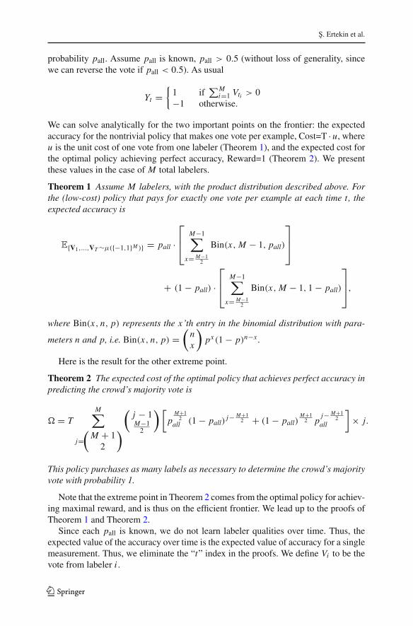
probability pall. Assume pall is known, pall > 0.5 (without loss of generality, sincewe can reverse the vote if pall < 0.5). As usual

Yt ={

1 if∑M

i=1 Vti > 0−1 otherwise.

We can solve analytically for the two important points on the frontier: the expectedaccuracy for the nontrivial policy that makes one vote per example, Cost=T · u, whereu is the unit cost of one vote from one labeler (Theorem 1), and the expected cost forthe optimal policy achieving perfect accuracy, Reward=1 (Theorem 2). We presentthese values in the case of M total labelers.

Theorem 1 Assume M labelers, with the product distribution described above. Forthe (low-cost) policy that pays for exactly one vote per example at each time t, theexpected accuracy is

E{V1,...,VT∼μ({−1,1}M )} = pall ·⎡⎢⎣

M−1∑x= M−1

2

Bin(x,M − 1, pall)

⎤⎥⎦

+ (1− pall) ·⎡⎢⎣

M−1∑x= M−1

2

Bin(x,M − 1, 1− pall)

⎤⎥⎦,

where Bin(x, n, p) represents the x’th entry in the binomial distribution with para-

meters n and p, i.e. Bin(x, n, p) =(

nx

)px (1− p)n−x .

Here is the result for the other extreme point.

Theorem 2 The expected cost of the optimal policy that achieves perfect accuracy inpredicting the crowd’s majority vote is

� = TM∑

j=(

M + 12

)(

j − 1M−1

2

)[p

M+12

all (1− pall)j− M+1

2 + (1− pall)M+1

2 pj− M+1

2all

]× j.

This policy purchases as many labels as necessary to determine the crowd’s majorityvote with probability 1.

Note that the extreme point in Theorem 2 comes from the optimal policy for achiev-ing maximal reward, and is thus on the efficient frontier. We lead up to the proofs ofTheorem 1 and Theorem 2.

Since each pall is known, we do not learn labeler qualities over time. Thus, theexpected value of the accuracy over time is the expected value of accuracy for a singlemeasurement. Thus, we eliminate the “t” index in the proofs. We define Vi to be thevote from labeler i .

123

Approximating the crowd

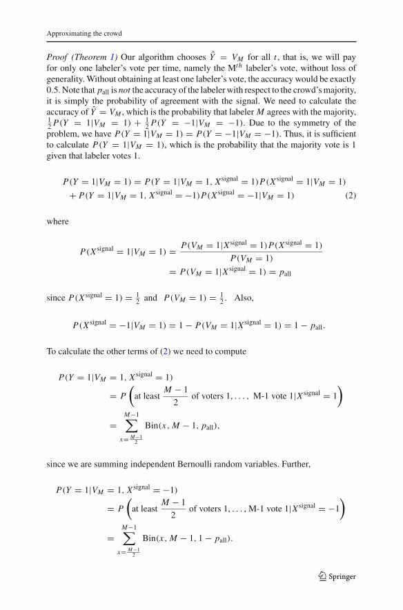
Proof (Theorem 1) Our algorithm chooses Y = VM for all t , that is, we will payfor only one labeler’s vote per time, namely the Mth labeler’s vote, without loss ofgenerality. Without obtaining at least one labeler’s vote, the accuracy would be exactly0.5. Note that pall is not the accuracy of the labeler with respect to the crowd’s majority,it is simply the probability of agreement with the signal. We need to calculate theaccuracy of Y = VM , which is the probability that labeler M agrees with the majority,12 P(Y = 1|VM = 1) + 1

2 P(Y = −1|VM = −1). Due to the symmetry of theproblem, we have P(Y = 1|VM = 1) = P(Y = −1|VM = −1). Thus, it is sufficientto calculate P(Y = 1|VM = 1), which is the probability that the majority vote is 1given that labeler votes 1.

P(Y = 1|VM = 1) = P(Y = 1|VM = 1, X signal = 1)P(X signal = 1|VM = 1)

+ P(Y = 1|VM = 1, X signal = −1)P(X signal = −1|VM = 1) (2)

where

P(X signal = 1|VM = 1) = P(VM = 1|X signal = 1)P(X signal = 1)

P(VM = 1)

= P(VM = 1|X signal = 1) = pall

since P(X signal = 1) = 12 and P(VM = 1) = 1

2 . Also,

P(X signal = −1|VM = 1) = 1− P(VM = 1|X signal = 1) = 1− pall.

To calculate the other terms of (2) we need to compute

P(Y = 1|VM = 1, X signal = 1)

= P

(at least

M − 1

2of voters 1, . . . , M-1 vote 1|X signal = 1

)

=M−1∑

x= M−12

Bin(x,M − 1, pall),

since we are summing independent Bernoulli random variables. Further,

P(Y = 1|VM = 1, X signal = −1)

= P

(at least

M − 1

2of voters 1, . . . , M-1 vote 1|X signal = −1

)

=M−1∑

x= M−12

Bin(x,M − 1, 1− pall).

123

S. Ertekin et al.

Putting it together,

P(Y = 1|VM = 1) =⎡⎢⎣

M−1∑x= M−1

2

Bin(x,M − 1, pall)

⎤⎥⎦ pall

+⎡⎢⎣

M−1∑x= M−1

2

Bin(x,M − 1, 1− pall)

⎤⎥⎦ (1− pall).

��

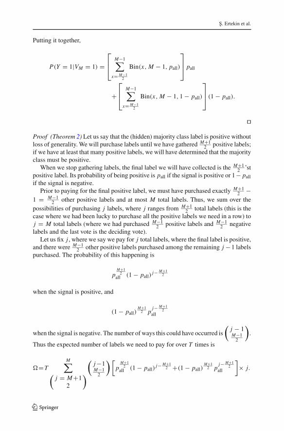
Proof (Theorem 2) Let us say that the (hidden) majority class label is positive withoutloss of generality. We will purchase labels until we have gathered M+1

2 positive labels;if we have at least that many positive labels, we will have determined that the majorityclass must be positive.

When we stop gathering labels, the final label we will have collected is the M+12 ’st

positive label. Its probability of being positive is pall if the signal is positive or 1− pallif the signal is negative.

Prior to paying for the final positive label, we must have purchased exactly M+12 −

1 = M−12 other positive labels and at most M total labels. Thus, we sum over the

possibilities of purchasing j labels, where j ranges from M+12 total labels (this is the

case where we had been lucky to purchase all the positive labels we need in a row) toj = M total labels (where we had purchased M−1

2 positive labels and M−12 negative

labels and the last vote is the deciding vote).Let us fix j , where we say we pay for j total labels, where the final label is positive,

and there were M−12 other positive labels purchased among the remaining j −1 labels

purchased. The probability of this happening is

pM+1

2all (1− pall)

j− M+12

when the signal is positive, and

(1− pall)M+1

2 pj− M+1

2all

when the signal is negative. The number of ways this could have occurred is

(j − 1M−1

2

).

Thus the expected number of labels we need to pay for over T times is

�=TM∑

(j = M+1

2

)(

j−1M−1

2

)[p

M+12

all (1− pall)j− M+1

2 +(1− pall)M+1

2 pj− M+1

2all

]× j.

123

Approximating the crowd

0.6 0.8 1

0.7

0.8

0.9

1

pall

E(A

ccur

acy)

from

The

orem

1

0.6 0.8 13

3.5

4

4.5

pall

E(C

ost)

from

The

orem

2

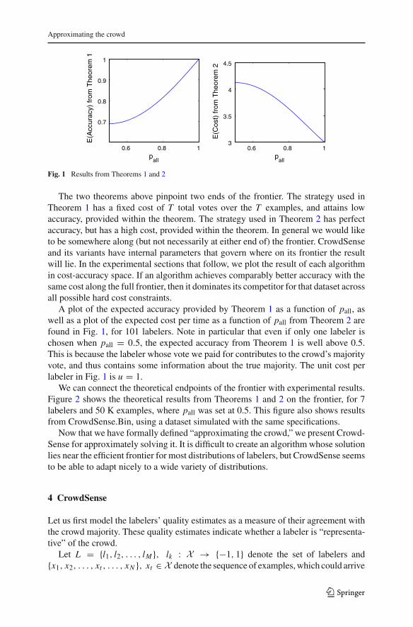
Fig. 1 Results from Theorems 1 and 2

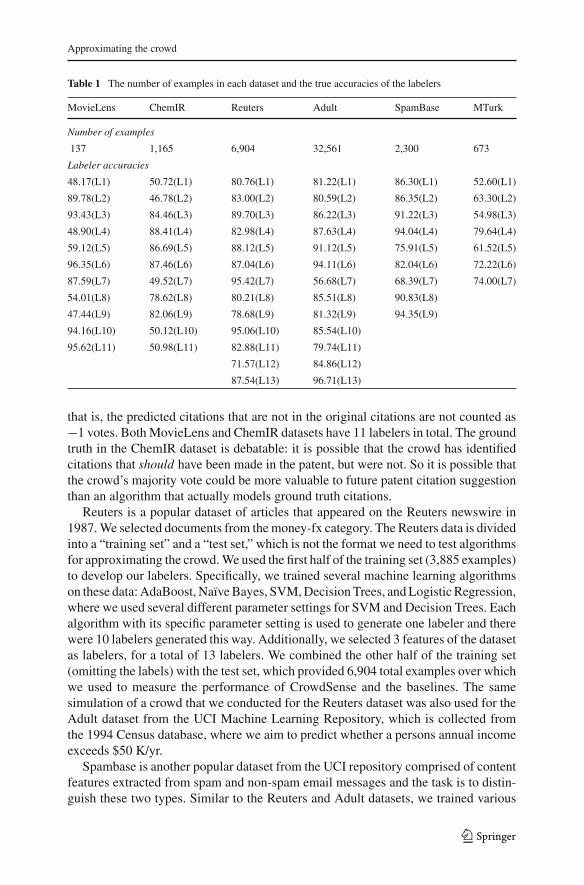
The two theorems above pinpoint two ends of the frontier. The strategy used inTheorem 1 has a fixed cost of T total votes over the T examples, and attains lowaccuracy, provided within the theorem. The strategy used in Theorem 2 has perfectaccuracy, but has a high cost, provided within the theorem. In general we would liketo be somewhere along (but not necessarily at either end of) the frontier. CrowdSenseand its variants have internal parameters that govern where on its frontier the resultwill lie. In the experimental sections that follow, we plot the result of each algorithmin cost-accuracy space. If an algorithm achieves comparably better accuracy with thesame cost along the full frontier, then it dominates its competitor for that dataset acrossall possible hard cost constraints.

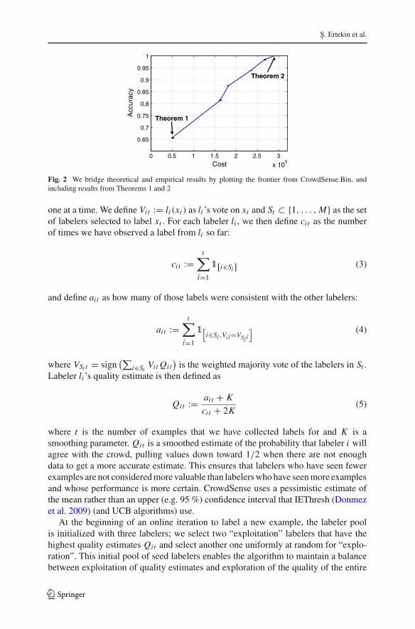
A plot of the expected accuracy provided by Theorem 1 as a function of pall, aswell as a plot of the expected cost per time as a function of pall from Theorem 2 arefound in Fig. 1, for 101 labelers. Note in particular that even if only one labeler ischosen when pall = 0.5, the expected accuracy from Theorem 1 is well above 0.5.This is because the labeler whose vote we paid for contributes to the crowd’s majorityvote, and thus contains some information about the true majority. The unit cost perlabeler in Fig. 1 is u = 1.

We can connect the theoretical endpoints of the frontier with experimental results.Figure 2 shows the theoretical results from Theorems 1 and 2 on the frontier, for 7labelers and 50 K examples, where pall was set at 0.5. This figure also shows resultsfrom CrowdSense.Bin, using a dataset simulated with the same specifications.

Now that we have formally defined “approximating the crowd,” we present Crowd-Sense for approximately solving it. It is difficult to create an algorithm whose solutionlies near the efficient frontier for most distributions of labelers, but CrowdSense seemsto be able to adapt nicely to a wide variety of distributions.

4 CrowdSense

Let us first model the labelers’ quality estimates as a measure of their agreement withthe crowd majority. These quality estimates indicate whether a labeler is “representa-tive” of the crowd.

Let L = {l1, l2, . . . , lM }, lk : X → {−1, 1} denote the set of labelers and{x1, x2, . . . , xt , . . . , xN }, xt ∈ X denote the sequence of examples, which could arrive

123

S. Ertekin et al.

0 0.5 1 1.5 2 2.5 3

x 105

0.65

0.7

0.75

0.8

0.85

0.9

0.95

1

Cost

Acc

urac

y

Theorem 1

Theorem 2

Fig. 2 We bridge theoretical and empirical results by plotting the frontier from CrowdSense.Bin, andincluding results from Theorems 1 and 2

one at a time. We define Vit := li (xt ) as li ’s vote on xt and St ⊂ {1, . . . ,M} as the setof labelers selected to label xt . For each labeler li , we then define cit as the numberof times we have observed a label from li so far:

cit :=t∑

t=1

1[i∈St ] (3)

and define ait as how many of those labels were consistent with the other labelers:

ait :=t∑

t=1

1[i∈St ,Vit=VSt t

] (4)

where VSt t = sign(∑

i∈StVit Qit

)is the weighted majority vote of the labelers in St .

Labeler li ’s quality estimate is then defined as

Qit := ait + K

cit + 2K(5)

where t is the number of examples that we have collected labels for and K is asmoothing parameter. Qit is a smoothed estimate of the probability that labeler i willagree with the crowd, pulling values down toward 1/2 when there are not enoughdata to get a more accurate estimate. This ensures that labelers who have seen fewerexamples are not considered more valuable than labelers who have seen more examplesand whose performance is more certain. CrowdSense uses a pessimistic estimate ofthe mean rather than an upper (e.g. 95 %) confidence interval that IEThresh (Donmezet al. 2009) (and UCB algorithms) use.

At the beginning of an online iteration to label a new example, the labeler poolis initialized with three labelers; we select two “exploitation” labelers that have thehighest quality estimates Qit and select another one uniformly at random for “explo-ration”. This initial pool of seed labelers enables the algorithm to maintain a balancebetween exploitation of quality estimates and exploration of the quality of the entire

123

Approximating the crowd

Algorithm 1 Pseudocode for CrowdSense.1. Input: Examples {x1, x2, . . . , xN }, Labelers {l1, l2, . . . , lM }, confidence threshold ε, smoothing para-

meter K .2. Initialize: ai1 ← 0, ci1 ← 0 for i = 1, . . . ,M and Qit ← 0 for i = 1 . . .M, t = 1 . . . N ,

L Q = {l(1), . . . , l(M)} random permutation of labeler id’s3. For t = 1, ..., N

(a) Compute quality estimates Qit = ait+Kcit+2K , i = 1, . . . ,M . Update L Q = {l(1), . . . , l(M)}, labeler

id’s in descending order of their quality estimates. If quality estimates are identical, randomlypermute labelers with identical qualities to attain an order.

(b) St = {l(1), l(2), l(k)}, where k is chosen uniformly at random from the set {3, . . .M}.(c) For j = 3 . . .M, j �= k

i. Score(St ) =∑i∈St

Vit Qit , lcandidate = l( j).

ii. If|Score(St )|−Qlcandidate,t|St |+1 < ε, then St ← St ∪ lcandidate. Otherwise exit loop to stop adding

new labelers to St .

(d) Return the weighted majority vote of the labelers: VSt t = sign(∑

i∈StVit Qit

)(e) ∀i ∈ St where Vit = VSt t , ait ← ait + 1(f) ∀i ∈ St , cit ← cit + 1

4. End

set of labelers. We ask each of these 3 labelers to vote on the example. The votesobtained from these labelers for this example are then used to generate a confidencescore, given as

Score(St ) =∑i∈St

Vit Qit

which represents the weighted majority vote of the labelers. Next, we determinewhether we are certain that the sign of Score(St ) reflects the crowd’s majority vote,and if we are not sure, we repeatedly ask another labeler to vote on this example untilwe are sufficiently certain about the label. To measure how certain we are, we greedilysee whether adding an additional labeler might make us uncertain about the decision.Specifically, we select the labeler with the highest quality estimate Qit , who is notalready in St , as a candidate to label this example. We then check whether this labelercould potentially either change the weighted majority vote if his vote were included,or if his vote could bring us into the regime of uncertainty where the Score(St ) isclose to zero, and the vote is approximately a tie. We check this before we pay forthis labeler’s vote, by temporarily assigning him a vote that is opposite to the currentsubcrowd’s majority. The criteria for adding the candidate labeler to St is defined as:

|Score(St )| − Qlcandidate,t

|St | + 1< ε (6)

where ε controls the level of uncertainty we are willing to permit, 0 < ε ≤ 1. If (6) istrue, the candidate labeler is added to St and we get (pay for) this labeler’s vote for xt .We then recompute Score(St ) and follow the same steps for the next-highest-qualitycandidate from the pool of unselected labelers. If the candidate labeler is not added toSt , we are done adding labelers for example t , and assign the weighted majority voteas the predicted label of this example. We then proceed to label the next example inthe collection. Pseudocode for the CrowdSense algorithm is given in Algorithm 1.

123

S. Ertekin et al.

5 Datasets and baselines

In order for us to evaluate the quality of a system for approximating the crowd, werequire databases with many examples, for which all of the labelers’ votes are knownon each example (so the majority can be calculated). This allows an unbiased, offlineevaluation to be performed. Ground truth labels may or may not be present; as inthe answer services applications, even if ground truth exists, we assume there is norealistic way to obtain it. One of the most commonly known crowdsourced databaseswas used in the Netflix Contest5. This database contains 100 million anonymous movieratings, and could definitely be used to predict the crowds opinion on movies, eventhough it was not explicitly designed for that purpose (however it is no longer publiclyavailable). For our experiments, we used various synthetic and real-world datasets thatmodel a crowd from two separate perspectives; the first perspective models the crowdin the traditional sense where the crowd comprises of human labelers, whereas thesecond perspective models the crowd in terms of competing predictive models and thegoal is to approximate the common prediction of these models.

This paper thus develops the largest collection of complete crowdsourced databasesavailable with the necessary characteristics for these types of experiments. We alsovaried the amount of various types of noise in the datasets, to account for a broadertype of data than is publicly available, and to provide a type of sensitivity analysis.The number of examples in each dataset and the true accuracies of the labelers areshown in Table 1. Our datasets are publicly available6.

All reported results are averages of 100 runs, each with a random ordering ofexamples to prevent bias due to the order in which examples are presented.

MovieLens is a movie recommendation dataset of user ratings on a collection ofmovies, and our goal is to find the majority vote of these reviewers. The dataset isoriginally very sparse, meaning that only a small subset of (human) users have ratedeach movie. We compiled a smaller subset of this dataset where each movie is ratedby each user in the subset, to enable comparative experiments, where labels can be“requested” on demand at a cost. We mapped the original rating scale of [0–5] tovotes of −1, 1 by using 2.5 as the threshold. The resulting dataset has the benefits ofhaving both human labelers and the completeness required to evaluate algorithms forapproximating the crowd. There is no ground truth in movie ratings, other than thecrowd’s majority vote.

ChemIR is a dataset of chemical patent documents from the 2009 TREC ChemistryTrack. This track defines a “Prior Art Search” task, where the competition is to developalgorithms that, for a given set of patents, retrieve other patents that they considerrelevant to those patents. The evaluation criteria is based on whether there is an overlapof the original citations of patents and the patents retrieved by the algorithm. TheChemIR dataset that we compiled is the complete list of citations of several chemistrypatents, and the +1,−1 votes indicate whether or not an algorithm has successfullyretrieved a true citation of a patent. In our dataset, we do not consider false positives;

5 http://www.netflixprize.com6 Dataset are available at http://github.com/CrowdSense/Datasets

123

Approximating the crowd

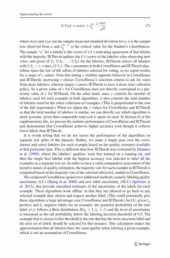
Table 1 The number of examples in each dataset and the true accuracies of the labelers

MovieLens ChemIR Reuters Adult SpamBase MTurk

Number of examples

137 1,165 6,904 32,561 2,300 673

Labeler accuracies

48.17(L1) 50.72(L1) 80.76(L1) 81.22(L1) 86.30(L1) 52.60(L1)

89.78(L2) 46.78(L2) 83.00(L2) 80.59(L2) 86.35(L2) 63.30(L2)

93.43(L3) 84.46(L3) 89.70(L3) 86.22(L3) 91.22(L3) 54.98(L3)

48.90(L4) 88.41(L4) 82.98(L4) 87.63(L4) 94.04(L4) 79.64(L4)

59.12(L5) 86.69(L5) 88.12(L5) 91.12(L5) 75.91(L5) 61.52(L5)

96.35(L6) 87.46(L6) 87.04(L6) 94.11(L6) 82.04(L6) 72.22(L6)

87.59(L7) 49.52(L7) 95.42(L7) 56.68(L7) 68.39(L7) 74.00(L7)

54.01(L8) 78.62(L8) 80.21(L8) 85.51(L8) 90.83(L8)

47.44(L9) 82.06(L9) 78.68(L9) 81.32(L9) 94.35(L9)

94.16(L10) 50.12(L10) 95.06(L10) 85.54(L10)

95.62(L11) 50.98(L11) 82.88(L11) 79.74(L11)

71.57(L12) 84.86(L12)

87.54(L13) 96.71(L13)

that is, the predicted citations that are not in the original citations are not counted as−1 votes. Both MovieLens and ChemIR datasets have 11 labelers in total. The groundtruth in the ChemIR dataset is debatable: it is possible that the crowd has identifiedcitations that should have been made in the patent, but were not. So it is possible thatthe crowd’s majority vote could be more valuable to future patent citation suggestionthan an algorithm that actually models ground truth citations.

Reuters is a popular dataset of articles that appeared on the Reuters newswire in1987. We selected documents from the money-fx category. The Reuters data is dividedinto a “training set” and a “test set,” which is not the format we need to test algorithmsfor approximating the crowd. We used the first half of the training set (3,885 examples)to develop our labelers. Specifically, we trained several machine learning algorithmson these data: AdaBoost, Naïve Bayes, SVM, Decision Trees, and Logistic Regression,where we used several different parameter settings for SVM and Decision Trees. Eachalgorithm with its specific parameter setting is used to generate one labeler and therewere 10 labelers generated this way. Additionally, we selected 3 features of the datasetas labelers, for a total of 13 labelers. We combined the other half of the training set(omitting the labels) with the test set, which provided 6,904 total examples over whichwe used to measure the performance of CrowdSense and the baselines. The samesimulation of a crowd that we conducted for the Reuters dataset was also used for theAdult dataset from the UCI Machine Learning Repository, which is collected fromthe 1994 Census database, where we aim to predict whether a persons annual incomeexceeds $50 K/yr.

Spambase is another popular dataset from the UCI repository comprised of contentfeatures extracted from spam and non-spam email messages and the task is to distin-guish these two types. Similar to the Reuters and Adult datasets, we trained various

123

S. Ertekin et al.

machine learning algorithms with various settings on half of the dataset, and usedtheir predictions on the other half as the votes for those examples. In total, our datasetcontains 2,300 examples, each voted on by 9 labelers.

Finally, we experimented with the HITSpam dataset7, which includes descriptionsof tasks posted on the Amazon Mechanical Turk marketplace. This dataset was com-piled by asking workers on Mechanical Turk to examine whether a task is “legitimate”or if the purpose of the task is to game social media metrics, such as asking workersto follow a user on Twitter, to “like” a video on YouTube, etc. This dataset contains5,840 tasks voted on by 135 labelers for a total of 28,354 votes. While the dataset islarge in terms of the total number of votes, there are very few tasks that have beenvoted on by the same set of labelers. Even if we consider the 5 labelers that havelabeled the most tasks, there are only 89 tasks that are voted on by all of them. Ifwe consider the top 7 labelers, there are no tasks that are voted on by all of them. Inorder to obtain a sizable set of tasks that have votes from all labelers, we proceeded asfollows: First, we identified pairs of labelers li and l j where both labelers have labeledat least 10 tasks in common, and the votes of li and l j on all common-labeled tasks areidentical. We considered such a pair as a single labeler, and the votes of this labelerwere set to the union of the labels of li and l j . From there, we selected the 7 labelersthat labeled the most tasks, and we selected the tasks that have been labeled by at least5 of the labelers. In total, there were 673 tasks that matched this criteria. For the casesin which a labeler had not labeled a task, we generated a label randomly according tothe labeler’s accuracy (i.e. agreement with the majority vote) on the tasks that she haslabeled.

For MovieLens, we added 50 % noise and for ChemIR we added 60 % noise to 5of the labelers to introduce a greater diversity of judgments. This is because all theoriginal labelers had comparable qualities and did not strongly reflect the diversity oflabelers and other issues that we aim to address. For the Reuters and Adult datasets, wevaried the parameters of the algorithms’ labelers, which are formed from classificationalgorithms, to yield predictions with varying performance.

We compared CrowdSense with several baselines: (a) the accuracy of the averagelabeler, represented as the mean accuracy of the individual labelers, (b) the accuracyof the overall best labeler in hindsight, and (c) the algorithm that selects just overhalf the labelers (i.e. �11/2� = 6 for ChemIR and MovieLens, �13/2� = 7 forReuters and Adult) uniformly at random, which combines the votes of labelers withno quality assessment using a majority vote. In Section C of the supplementary file, wealso discuss the possibility of learning the labelers’ quality estimates using machinelearning.

Another baseline that we use to compare CrowdSense is IEThresh (Donmez et al.2009). IEThresh builds upon Interval Estimation (IE) learning, and estimates an upperconfidence interval UI for the mean reward for an action, which is a technique used inreinforcement learning. In IEThresh, an action refers to asking a labeler to vote on anitem, and a reward represents the labeler’s agreement with the majority vote. The U Imetric for IEThresh is defined for a sample “a” as:

7 http://github.com/ipeirotis/Get-Another-Label/tree/master/data/HITspam-UsingMTurk

123

Approximating the crowd

U I (a) = m(a)+ t (n−1)α2

s(a)√n

(7)

where m(a) and s(a) are the sample mean and standard deviation for a, n is the samplesize observed from a and t (n−1)

α2

is the critical value for the Student’s t-distribution.

The sample “a” for a labeler is the vector of±1’s indicating agreement of that labelerwith the majority. IEThresh updates the U I scores of the labelers after observing newvotes, and given {U I1,U I2, . . . ,U Ik} for the labelers, IEThresh selects all labelerswith U I j > ε×max j (U I j ). The ε parameter in both CrowdSense and IEThresh algo-rithms tunes the size of the subset of labelers selected for voting, so we report resultsfor a range of ε values. Note that tuning ε exhibits opposite behavior in CrowdSenseand IEThresh; increasing ε relaxes CrowdSense’s selection criteria to ask for votesfrom more labelers, whereas larger ε causes IEThresh to have a more strict selectionpolicy. So a given value of ε for CrowdSense does not directly correspond to a par-ticular value of ε for IEThresh. On the other hand, since ε controls the number oflabelers used for each example in both algorithms, it also controls the total numberof labelers used for the entire collection of examples. (This is proportional to the costof the full experiment.) When we adjust the ε values for CrowdSense and IEThreshso that the total number of labelers is similar, we can directly see which algorithm ismore accurate, given that comparable total cost is spent on each. In Section D of thesupplementary file, we present the runtime performance of CrowdSense and IEThreshand demonstrate that CrowdSense achieves higher accuracy even though it collectsfewer labels than IEThresh.

It is worth noting that we do not assess the performance of the algorithms onseparate test splits of the datasets. Rather, we make a single pass over the entiredataset and select labelers for each example based on the quality estimates availableat that particular time. This is different than how IEThresh was evaluated by Donmezet al. (2009), where the labelers’ qualities were first learned on a training set, andthen the single best labeler with the highest accuracy was selected to label all theexamples in a separate test set. In order to have a valid comparative assessment of theiterative nature of quality estimation, the majority vote for each example in IEThresh iscomputed based on the majority vote of the selected subcrowd, similar to CrowdSense.

We compared CrowdSense against two additional methods, namely labeling qualityuncertainty (LU) (Sheng et al. 2008) and new label uncertainty (NLU) (Ipeirotis etal. 2013), that provide smoothed estimates of the uncertainty of the labels for eachexample. These algorithms work offline, in that they are allowed to go back to anyselected example they choose and request another label. (This could potentially givethese algorithms a large advantage over CrowdSense and IEThresh.) In LU, given l p

positive and ln negative labels for an example, the posterior probability of the truelabel p(y) follows a Beta distribution B(l p + 1, ln + 1) and the level of uncertaintyis measured as the tail probability below the labeling decision threshold of 0.5. Theexample that is closest to this threshold is the one that has the most uncertain label andthe next set of labels should be selected for this instance. This calculation makes theapproximation that all labelers have the same quality when labeling a given example,which is not an assumption of CrowdSense.

123

S. Ertekin et al.

For NLU, any example that we have observed l p > ln labels has the posteriorprobability for the positive class

Pr(+|l p, ln) =(

1+ 1− Pr(+)Pr(+) ·

((ln + l p)!

)2

(2ln)! · (2l p)!

)−1

where Pr(+) denotes the prior for the positive class that can be computed iterativelyusing a marginal maximum likelihood algorithm. For examples with ln > l p labels,the posterior above is symmetric. Similar to the LU case, the example with the mostuncertain label is the one that has the score closest to 0.5 and the algorithm queries fornew labels for that example in the next iteration. We used the setting of LU and NLUas they are presented in (Sheng et al. 2008) and (Ipeirotis et al. 2013) respectively.

6 Overall performance

We compare CrowdSense with the baselines to demonstrate its ability to accuratelyapproximate the crowd’s vote. Accuracy is calculated as the proportion of exampleswhere the algorithm agreed with the majority vote of the entire crowd.

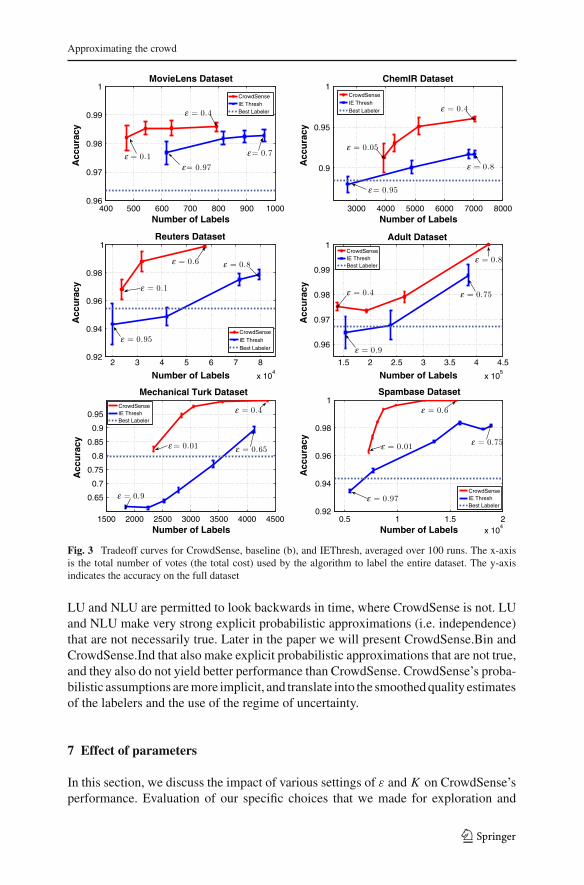
Figure 3 shows the comparison of CrowdSense against baseline (b) and IEThresh.On the subplots in Fig. 3, the accuracy of the best labeler in hindsight (baseline (b))is indicated as a straight line. Note that the accuracy of the best labeler is computedseparately as a constant. Baselines (a) and (c), which are the average labeler and theunweighted random labelers, achieved performance beneath that of the best labeler.For the MovieLens dataset, the values for these baselines are 74.05 and 83.69 %respectively; for ChemIR these values are 68.71 and 73.13 %, for Reuters, 84.84 and95.25 %, for Adult 83.94 and 95.03 %, for Mechanical Turk 65.46 and 77.12 %, and forSpambase the values are 85.49 and 93.43 %. The results indicate that uniformly acrossdifferent values of ε, CrowdSense consistently achieved the highest accuracy againstthese baselines, indicating that CrowdSense uses any fixed budget more effectivelythan the baselines. Generally, the quality estimates of CrowdSense better reflect thetrue accuracy of the members of the crowd and therefore, it can identify and picka more representative subset of the crowd. Also, the results demonstrate that askingfor labels from labelers at random may yield poor performance for representing themajority vote, highlighting the importance of making informed decisions for selectingthe representative members of the crowd. Asking the best and average labeler werealso not effective approximators of the majority vote.

For the LU and NLU experiments, we initialized both algorithms by randomlyselecting three labelers and acquiring their votes on each example in the dataset. Ateach round of collecting more labels for the most uncertain example, we acquired twoadditional labels to prevent ties. We did not specify a stopping criteria for either LU orNLU, so both algorithms ran until acquiring all labels for all examples in the dataset(therefore both algorithms eventually converge to 100 % accuracy). The comparisonof CrowdSense with LU and NLU is presented in Fig. 4. The results demonstrate thatCrowdSense achieves better general performance, where its impact is most pronouncedon the MovieLens, ChemIR, Mechanical Turk and Spambase datasets. We remark that

123

Approximating the crowd

400 500 600 700 800 900 10000.96

0.97

0.98

0.99

1MovieLens Dataset

Number of Labels

Acc

ura

cy

CrowdSenseIE ThreshBest Labeler

ε = 0.1ε= 0.97

ε = 0.4

ε= 0.7

3000 4000 5000 6000 7000 8000

0.9

0.95

1ChemIR Dataset

Number of Labels

Acc

ura

cy

CrowdSenseIE ThreshBest Labeler

ε = 0.05

ε = 0.95

ε = 0.4

ε = 0.8

2 3 4 5 6 7 8

x 104

0.92

0.94

0.96

0.98

1Reuters Dataset

Number of Labels

Acc

ura

cy

CrowdSense

IE Thresh

Best Labeler

ε = 0.1

ε = 0.6 ε = 0.8

ε = 0.95

1.5 2 2.5 3 3.5 4 4.5

x 105

0.96

0.97

0.98

0.99

1Adult Dataset

Number of Labels

Acc

ura

cy

CrowdSenseIE ThreshBest Labeler

ε = 0.4

ε = 0.9

ε = 0.8

ε = 0.75

1500 2000 2500 3000 3500 4000 4500

0.65

0.7

0.75

0.8

0.85

0.9

0.95

Mechanical Turk Dataset

Number of Labels

Acc

ura

cy

CrowdSenseIE ThreshBest Labeler

ε = 0.9

ε = 0.01 ε = 0.65

ε = 0.4

0.5 1 1.5 2x 10

4

0.92

0.94

0.96

0.98

1Spambase Dataset

Number of Labels

Acc

ura

cy

CrowdSenseIE ThreshBest Labeler

ε = 0.97

ε = 0.01

ε = 0.6

ε = 0.75

Fig. 3 Tradeoff curves for CrowdSense, baseline (b), and IEThresh, averaged over 100 runs. The x-axisis the total number of votes (the total cost) used by the algorithm to label the entire dataset. The y-axisindicates the accuracy on the full dataset

LU and NLU are permitted to look backwards in time, where CrowdSense is not. LUand NLU make very strong explicit probabilistic approximations (i.e. independence)that are not necessarily true. Later in the paper we will present CrowdSense.Bin andCrowdSense.Ind that also make explicit probabilistic approximations that are not true,and they also do not yield better performance than CrowdSense. CrowdSense’s proba-bilistic assumptions are more implicit, and translate into the smoothed quality estimatesof the labelers and the use of the regime of uncertainty.

7 Effect of parameters

In this section, we discuss the impact of various settings of ε and K on CrowdSense’sperformance. Evaluation of our specific choices that we made for exploration and

123

S. Ertekin et al.

400 600 800 1000 1200

0.85

0.9

0.95

1MovieLens Dataset

Number of Labels

Acc

ura

cy

CrowdSense

LU

NLU

ε = 0.4ε = 0.1

4000 6000 8000 10000 120000.75

0.8

0.85

0.9

0.95

1ChemIR Dataset

Number of Labels

Acc

ura

cy

CrowdSenseLUNLU

ε = 0.05

ε = 0.4

2 3 4 5 6 7x 10

4

0.9

0.92

0.94

0.96

0.98

1Reuters Dataset

Number of Labels

Acc

ura

cy

CrowdSenseLUNLU

ε = 0.6ε = 0.1

1.5 2 2.5 3 3.5 4 4.5x 10

5

0.92

0.94

0.96

0.98

1Adult Dataset

Number of Labels

Acc

ura

cy

CrowdSenseLUNLU

ε = 0.8ε = 0.4

2000 2500 3000 3500 4000 4500 50000.7

0.75

0.8

0.85

0.9

0.95

1Mechanical Turk Dataset

Number of Labels

Acc

ura

cy

CrowdSenseLUNLU

ε = 0.01

ε = 0.4

0.5 1 1.5 2x 10

4

0.92

0.94

0.96

0.98

1Spambase Dataset

Number of Labels

Acc

ura

cy

CrowdSenseLUNLU

ε = 0.6ε = 0.01

Fig. 4 Tradeoff curves for CrowdSense, LU and NLU, averaged over 100 runs. The x-axis is the totalnumber of votes (the total cost) used by the algorithm to label the entire dataset. The y-axis indicates theaccuracy on the full dataset

exploitation in the different components of CrowdSense is presented in Sect. 8. Wealso present experimental results that demonstrate the effect of initialization with goldstandard data in Section E of the supplementary file.

7.1 Effect of the ε parameter

As discussed throughout Sects. 4 and 5, the ε parameter is a trade-off between thetotal cost that we are willing to spend and the accuracy that we would like to achieve.Figure 5 illustrates the average running performance over 100 runs of CrowdSense forvarious values of epsilon. Each final point on each of the Fig. 5 curves correspondsto a single point in Fig. 3. Figure 5 shows that over the full time course, increasingepsilon leads to increased accuracy, at a higher cost.

123

Approximating the crowd

20 40 60 80 100 120 1400.94

0.95

0.96

0.97

0.98

0.99

1MovieLens Dataset

Number of Examples

Ru

nn

ing

Acc

ura

cy

ε = 5 × 10−3

ε = 0.01ε = 0.1ε = 0.2

437439

476 541

0 200 400 600 800 1000 12000.88

0.9

0.92

0.94

0.96

0.98

1ChemIR Dataset

Number of Examples

Ru

nn

ing

Acc

ura

cy

ε = 5 × 10−3

ε = 0.01ε = 0.1ε = 0.2

5132

4294

3797

3775

0 2000 4000 6000 80000.86

0.88

0.9

0.92

0.94

0.96

0.98

1Reuters Dataset

Number of Examples

Ru

nn

ing

Acc

ura

cy

ε = 5 × 10−3

ε = 0.01ε = 0.1ε = 0.2

21,573

21,73823,766

26,032

0 1 2 3x 10

4

0.86

0.88

0.9

0.92

0.94

0.96

0.98Adult Dataset

Number of Examples

Ru

nn

ing

Acc

ura

cy

ε = 5 × 10−3

ε = 0.01ε = 0.1ε = 0.2

1 × 105

1.07 × 1051.15 × 105

Fig. 5 Comparison of the running accuracy of CrowdSense at various ε values, averaged over 100 runs.In the plots, we show how many total votes were requested at each ε value

7.2 Effect of the K parameter

The K parameter helps with both exploration at early stages and exploitation at laterstages. In terms of exploration, K ensures that labelers who have seen fewer examples(smaller cit ) are not considered more valuable than labelers who have seen manyexamples. The quality estimate in (5) is a shrinkage estimator, lowering probabilitieswhen there is uncertainty. Consider a labeler who was asked to vote on just oneexample and correctly voted. His vote should not be counted as highly as a voter whohas seen 100 examples and correctly labeled 99 of them. This can be achieved usingK sufficiently large.

Increasing K also makes the quality estimates more stable, which helps to permitexploration. Since the quality estimates are all approximately equal in early stages,the weighted majority vote becomes almost a simple majority vote. This preventsCrowdSense from trusting any labeler too much early on. Having the Qit ’s be almostequal also increases the chance to put CrowdSense into the “regime of uncertainty”where it requests more votes per example, allowing it to explore the labelers more.

We demonstrate the impact of K by comparing separate runs of CrowdSense withdifferent K in Fig. 6. Considering the MovieLens dataset, at K = 100, the qualityestimates tilt the selection criteria towards an exploratory scheme in most of the itera-tions. At the other extreme, K = 0 causes the quality estimates to be highly sensitive

123

S. Ertekin et al.

20 40 60 80 100 120 1400.9

0.92

0.94

0.96

0.98

MovieLens Dataset

Number of Examples

Ru

nn

ing

Acc

ura

cy

K=0K=10K=100

437 446

459

0 200 400 600 800 1000 1200

0.4

0.5

0.6

0.7

0.8

0.9

1

Number of Examples

Ru

nn

ing

Acc

ura

cy

ChemIR Dataset

K=0K=10K=100

3866

3781

3793

0 1000 2000 3000 4000 5000 6000 70000.87

0.88

0.89

0.9

0.91

0.92

0.93

0.94Reuters Dataset

Number of Examples

Ru

nn

ing

Acc

ura

cy

K=0K=10K=100

21508

21648

21894

0 1 2 3x 10

4

0.86

0.88

0.9

0.92

0.94

Adult Dataset

Number of Examples

Ru

nn

ing

Acc

ura

cy

K=0K=10K=100

1.01 × 105

1 × 105

Fig. 6 Comparison of running accuracy with varying K. All curves use ε = 0.005, and are averaged over100 runs

to the accuracy of the labels right from the start. Furthermore, it is also interesting tonote that removing K achieves worse performance than K = 10 despite collectingslightly more votes. This indicates that the results are better when more conservativequality estimates are used in early iterations.

8 Specific choices for exploration and exploitation in CrowdSense

The algorithm template underlying CrowdSense has three components that can beinstantiated in different ways: (i) the composition of the initial seed set of labelers(step 4(b) in the pseudocode), (i i) how subsequent labelers are added to the set (step4(c)), and (i i i) the weighting scheme, that is, the quality estimates. This weightingscheme affects the selection of the initial labeler set, the way the additional labelersare incorporated, as well as the strategy for combining the votes of the labelers (steps4(b)(c)(d)).

Our overall results of this section are the algorithm is fairly robust to components(i) and (i i), but not to component (i i i): the weighting scheme is essential, but chang-ing the composition of the seed set and the way subsequent labelers are added doesnot heavily affect accuracy. There is a good reason why CrowdSense is robust tochanges in (i) and (i i). CrowdSense already has an implicit mechanism for explo-ration, namely the smoothing done on the estimates of quality, discussed in Sect. 7.2,

123

Approximating the crowd

0 100 200 300 400 5000.8

0.84

0.88

0.92

0.96

Number of Labels

Ru

nn

ing

Acc

ura

cyMovieLens Dataset

0 1000 2000 3000 4000

0.75

0.8

0.85

0.9

ChemIR Dataset

Number of Labels

Ru

nn

ing

Acc

ura

cy

CrowdSense

3Q

1Q

0Q

Component 2

No Weights

LCI

Component 1

Component 3

0 0.5 1 1.5 2 2.5 3x 10

4

0.94

0.96

0.98

1Reuters Dataset

Number of Labels

Ru

nn

ing

Acc

ura

cy

0 2 4 6 8 10 12x 10

4

0.82

0.84

0.86

0.88

0.9

0.92

0.94

0.96Adult Dataset

Number of Labels

Ru

nn

ing

Acc

ura

cy

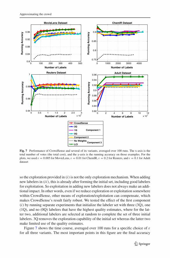
Fig. 7 Performance of CrowdSense and several of its variants, averaged over 100 runs. The x-axis is thetotal number of votes (the total cost), and the y-axis is the running accuracy on those examples. For theplots, we used ε = 0.005 for MovieLens, ε = 0.01 for ChemIR, ε = 0.2 for Reuters, and ε = 0.1 for Adultdataset

so the exploration provided in (i) is not the only exploration mechanism. When addingnew labelers in (i i), this is already after forming the initial set, including good labelersfor exploitation. So exploitation in adding new labelers does not always make an addi-tional impact. In other words, even if we reduce exploration or exploitation somewherewithin CrowdSense, other means of exploration/exploitation can compensate, whichmakes CrowdSense’s result fairly robust. We tested the effect of the first component(i) by running separate experiments that initialize the labeler set with three (3Q), one(1Q), and no (0Q) labelers that have the highest quality estimates, where for the lat-ter two, additional labelers are selected at random to complete the set of three initiallabelers. 3Q removes the exploration capability of the initial set whereas the latter twomake limited use of the quality estimates.

Figure 7 shows the time course, averaged over 100 runs for a specific choice of εfor all three variants. The most important points in this figure are the final accuracy

123

S. Ertekin et al.

of final total number of labels (i.e. the budget). Note that each variant implementsa separate labeler selection and/or label weighting scheme which, in turn, affectsthe total number of labels collected by each variant. Some of the datasets (Reuters,ChemIR) did not show much change. The MovieLens dataset, the smallest dataset inour experiments, shows the largest gain in the predictive performance of CrowdSensecompared to the other three variants. This is also the dataset where the difference inthe number of labels collected for each curve is reasonably comparable across thevariants—so for the same total budget, the performance of CrowdSense was better.For the Adult dataset, 1Q achieves the highest final accuracy, but it also collects closeto 10 K more labels than CrowdSense, so the accuracies are not directly comparablebecause the budget is different. This agrees with the compromise that we discussedin the Introduction, regarding the decisions on how to spend the budget on collectinglabels.

We experimented with the second component (i i) by adding labelers randomlyrather than in order of their qualities. In this case, exploitation is limited, and thealgorithm again tends not to perform as well on most datasets (as shown in Fig. 7 forthe curve marked “Component 2”) either in terms of accuracy or budget.

To test the effect of the weighting scheme in the third component (i i i), we firstremoved the use of weights from the algorithm. This corresponds to selecting theinitial seed of labelers and the additional labelers at random without using their qualityestimates. In addition, when combining the votes of the individual labelers, we usemajority voting, rather than a weighted majority vote. This approach performs theworst among all the variants in all four datasets, demonstrating the significance ofusing quality estimates for labeler selection and the calculation of the weighted vote.

We also experimented with a separate scoring scheme for estimating the labelerqualities. In particular, we estimated labeler i’s quality at iteration t using a lower con-fidence interval. The lower confidence limit at level α, using the normal approximationto the binomial is:

Qit = pi t − z1− 12α

√1

cipi t (1− pi t ) (8)

where pi t = aitci t

is the proportion of labeler i’s labels that were consistent with theother labelers. The definition and computation of a and c were presented in Sect. 3. InFigure 7, the curve with the label LCI shows the running accuracy results for estimatingthe labelers’ qualities using this scheme at α = 0.25. The results are comparable toCrowdSense, performing similarly in some datasets, better in one, and worse thananother, indicating that (8) is a reasonable alternative to the choice of labeler qualityestimates for the weighting scheme.

9 Probabilistic algorithms for approximating the crowd

CrowdSense has four important properties: (1) It takes labelers’ votes into accounteven if they are right only half of the time. This property is especially beneficial forapproximating small crowds, (2) It trusts “better” labelers more, and places higher

123

Approximating the crowd

emphasis on their votes, (3) Its decision rule is derived to be similar to boosting,and (4) smoothing of the quality estimates. These estimates provide the means forexploration of labelers in the earlier stages, and exploitation in later stages.

The fact that the majority vote determines the ground truth indicates a complicatedrelationship, a joint probability distribution, between the labelers’ accuracies withrespect to the majority vote. CrowdSense makes an implicit approximation on thejoint probability distribution through its boosting-style update. We believe it is possi-ble to further improve its accuracy by making an explicit approximation on the jointprobability distribution. To that effect, we propose two variations of CrowdSense thatdirectly incorporate the joint probability distributions of the labelers under differentapproximations. These algorithms are designed to bring probabilistic insight into theworkings of CrowdSense and other algorithms for approximating the crowd. The firstvariation (CrowdSense.Ind) makes a statistical independence approximation for thelabelers. That is, we will assume that the majority vote is approximately independentof the votes that we have seen so far. This approximation is useful for large crowds, butmay not be useful for smaller crowds. CrowdSense.Ind’s probabilistic interpretationreplaces the boosting-style update to improve upon property 3; however, it sacrificesproperty 1. Therefore, its benefits are geared towards large crowds. The second varia-tion (CrowdSense.Bin) makes a different probabilistic approximation, which is a lowerbound on how often the current subcrowd agrees with the majority vote. This leads to adifferent voting scheme which is based on the binomial distribution of the votes. Thisalso replaces the boosting-style decision rule in property 3. CrowdSense.Bin does notinclude the current subcrowd’s weights in the vote, but the labeler selection criteriastill favors labelers with high accuracy. Consequently, this approach covers the secondproperty to some extent, but not as strong as the original CrowdSense.

9.1 CrowdSense.Ind

CrowdSense.Ind assumes that the quality of the individual labelers gives much moreinformation than the count of votes received so far. In other words, that a labelerwho is right 90 % of the time and votes +1 should be counted more than a handfulof mediocre labelers who vote −1. This can be approximately true when there alarge number of labelers, but is not true for a small number of labelers. For instance,consider a case where we have received three votes so far: [+1,−1,−1], from labelerswith qualities 0.8, 0.5, and 0.5 respectively. Let’s say that there are a total of 500labelers. The evidence suggests that the majority vote will be +1, in accordance withthe high quality voter, and discounting the low-quality labelers. This is the type ofapproximation CrowdSense.Ind makes. Instead, if there were only 5 labelers total,evidence suggests that the majority vote might be −1, since the low quality labelersstill contribute to the majority vote, and only one more −1 vote is now needed to geta majority.

Let Vi denote the vote of labeler i on a particular example, and Pi denote theprobability that the labeler will agree with the crowd’s majority vote. Consider thattwo labelers have voted 1 and −1, and we want to evaluate the probability that themajority vote is 1. Then, from Bayes Rule, we have

123

S. Ertekin et al.

P(y = 1|V1 = 1, V2 = −1) = P(V1 = 1, V2 = −1, y = 1)

P(V1 = 1, V2 = −1)P(V1 = 1, V2 = −1, y = 1) = P(y = 1)P(V1 = 1, V2 = −1|y = 1)

= P(y = 1)P(V1 = Vmaj , V2 �= Vmaj )

= P(y = 1)P1(1− P2)

P(V1 = 1, V2 = −1) = P(y = 1)P(V1 = 1, V2 = −1|y = 1)

+ P(y = −1)P(V1 = 1, V2 = −1|y = −1)

P(y = 1|V1 = 1, V2 = −1) = P1(1− P2)P(y = 1)

P(y = 1)P1(1− P2)+ P(y = −1)(1− P1)P2

where P(y = 1) and P(y = −1) are the ratios of the crowd’s approximated votes of1 and −1 on the examples voted so far, respectively.

To expand this more generally to arbitrary size subsets of crowds, we define thefollowing notation: Let V bin

i denote the mapping of labeler i’s vote from {−1, 1} to{0, 1}, i.e. V bin

i = (Vi + 1)/2. Using the following notation for the joint probabilitiesof agreement and disagreement with the crowd:

ψi = PV bin

ii (1− Pi )

1−V bini (probability of agreement given vote Vbin)

θi = (1− Pi )V bin

i P1−V bin

ii (probability of disagreement given vote Vbin)

the likelihood of the majority vote y being 1 is estimated by the following conditionalprobability:

f (xt |votes) = P(y = 1| V1, V2, . . . , Vi︸ ︷︷ ︸votes of labelers in S

) =(∏

l∈S ψl)

P+(∏l∈S ψl

)P+ +

(∏l∈S θl

)(1− P+)

= 1

1+(∏

l∈S θl)(1− P+)(∏

l∈S ψl)

P+

(9)

where probabilities higher than 0.5 indicate a majority vote estimate of 1, and −1otherwise. Further, the more the probability in (9) diverges from 0.5, the more we areconfident of the current approximation of the crowd based on the votes seen so far.

Note that labelers who are accurate less than half the time can be “flipped” so theopposite of their votes are used. That is, observing a vote Vi with Pi < 0.5 is equivalentto observing −Vi with probability 1− Pi . In Section B of the supplementary file, wediscuss about this flipping heuristics and present graphs that demonstrate the effect ofthis approach.

As in CrowdSense, the decision of whether or not to get a vote from an additionallabeler depends on whether his vote could bring us to the regime of uncertainty. Asin CrowdSense, this corresponds to hypothetically getting a vote from the candidatelabeler that disagrees with the current majority vote. This corresponds to hypotheticallygetting a -1 vote when P(y = 1|votes) > 0.5, and getting a 1 vote otherwise. Defining

123

Approximating the crowd

Fig. 8 The confidence intervalsof the probabilistic approachwith the independenceapproximation of the labelers

ψcandidate ={

1− Pcandidate f (xt |votes) > 0.5Pcandidate otherwise

θcandidate ={

Pcandidate f (xt |votes) > 0.51− Pcandidate otherwise

and expanding (9) to include the new hypothetical vote from the candidate labeler, weget

f (xt |votes, Vcandidate) = 1

1+(∏

l∈S θl)θcandidate (1− P+)(∏

l∈S ψl)ψcandidate P+

. (10)

The decision as to whether get a new vote depends on the values of Eqs. (9) and (10).If we are sufficiently confident of the current majority vote to the point where the nextbest labeler we have could not change our view, or is not in the regime of uncertainty(shown in Fig. 8), then we simply make a decision and do not call any more votes.Pseudocode of CrowdSense.Ind is in Algorithm 2.

9.2 CrowdSense.Bin

The statistical independence approximation that we made in Sect. 9.1 is useful forsufficiently large crowds, but it is not a useful approximation when the crowd issmall. In this subsection, we modify our treatment of the joint probability distribution.Specifically, we estimate a lower bound on how often the subcrowd St agrees with thecrowd’s majority vote.

Consider again the scenario where there are 5 labelers in the crowd, and we alreadyhave observed [+1,−1,−1] votes from three labelers. The simple majority of thecrowd would be determined by 3 votes in agreement, and we already have two votesof −1. So the problem becomes estimating the likelihood of getting one more voteof −1 from the two labelers that have not voted yet, which is sufficient to determinethe simple majority vote. If the voters are independent, this can be determined froma computation on the binomial distribution. Let Nneeded denote the number of votesneeded for a simple majority and let Nunvoted denote the number of labelers that havenot yet voted. (In the example above with 5 labelers, Nneeded = 1 and Nunvoted = 2). Inorder to find a lower bound, we consider what happens if the remaining labelers havethe worst possible accuracy, P = 0.5. We then define the score using the probability ofgetting enough votes from the remaining crowd that agree with the current majorityvote:

123

S. Ertekin et al.

Algorithm 2 Pseudocode for CrowdSense.Ind.1. Input: Examples {x1, x2, . . . , xN }, Labelers {l1, l2, . . . , lM }, confidence threshold ε, smoothing para-

meter K .2. Initialize: ai1 ← 0, ci1 ← 0 for i = 1, . . . ,M and Qit ← 0 for i = 1 . . .M, t = 1 . . . N ,

L Q = {l(1), . . . , l(M)} random permutation of labeler id’s3. Loop for t = 1, ..., N

(a) Compute quality estimates Qit = ait+Kcit+2K , i = 1, . . . ,M . Update L Q = {l(1), . . . , l(M)}, labeler

id’s in descending order of their quality estimates. If quality estimates are identical, randomlypermute labelers with identical qualities to attain an order.

(b) Select 3 labelers and get their votes. St = {l(1), l(2), l(k)}, where k is chosen uniformly at randomfrom the set {3, . . . ,M}.

(c) V bini t = (Vit+1)

2 , ∀i ∈ St

(d) ψi t = QV bin

i ti t (1− Qit )

1−V bini t , ∀i ∈ St

(e) θi t = (1− Qit )V bin

i t Q1−V bin

i ti t , ∀i ∈ St

(f) Loop for candidate = 3 . . .M, candidate �= k

i. f (xt |votes) = 1

1+ (∏

i∈Stθi t )(1− P+)

(∏

i∈Stψi t )P+

, where P+ is the probability of a +1 majority

vote.ii. ψcandidate = 1− Qcandidate,t

iii. θcandidate = Qcandidate,t

iv. f (xt |votes, Vcandidate,t ) = 1

1+ (∏

i∈Stθi t )θcandidate(1− P+)

(∏

i∈Stψi t )ψcandidate P+

v. If f (xt |votes) ≥ 0.5 and f (xt |votes, Vcandidate,t ) < 0.5+ ε then ShouldBranch = 1vi. If f (xt |votes) < 0.5 and f (xt |votes, Vcandidate,t ) > 0.5− ε then ShouldBranch = 1

vii. If ShouldBranch = 1 then St = {St ∪ candidate}, get the candidate’s vote. else Don’t needmore labelers, break out of loop.

(g) yt = 2× 1[ f (xt |votes)>0.5] − 1(h) ait = ait + 1, ∀i ∈ St where Vit = yt(i) cit = cit + 1, ∀i ∈ St

4. End

Score = PX∼Bin(·,Nunvoted,0.5)(X ≥ Nneeded)− 0.5

=⎡⎣ Nunvoted∑

X=Nneeded

Bin(X, Nunvoted, 0.5)

⎤⎦− 0.5, (11)

where Bin(X, Nunvoted, 0.5) is the Xth entry in the Binomial distribution with para-meters Nunvoted and probability of success of 0.5. In other words, this score representsa lower bound on how confident we are that the breakdown of votes that we haveobserved so far is consistent with the majority vote. The score (11) is always nonneg-ative; this is shown in Section A of the supplementary file. Therefore, the decision toask for a new vote can then be tied to our level of confidence, and if it drops belowa certain threshold ε, we can ask for the vote of the highest quality labeler that hasnot voted yet. The algorithm stops asking for additional votes once we are sufficientlyconfident that the subset of labels that we have observed is a good approximation ofthe crowd’s vote. The pseudocode of this approach is given in Algorithm 3.

123

Approximating the crowd

Algorithm 3 Pseudocode for CrowdSense.Bin1. Input: Examples {x1, x2, . . . , xN }, Labelers {l1, l2, . . . , lM }, confidence threshold ε, smoothing para-

meter K .2. Initialize: ai1 ← 0, ci1 ← 0 for i = 1, . . . ,M and Qit ← 0 for i = 1 . . .M, t = 1 . . . N ,

L Q = {l(1), . . . , l(M)} random permutation of labeler id’s3. For t = 1, ..., N

(a) Compute quality estimates Qit = ait+Kcit+2K , i = 1, . . . ,M . Update L Q = {l(1), . . . , l(M)}, labeler

id’s in descending order of their quality estimates. If quality estimates are identical, randomlypermute labelers with identical qualities to attain an order.

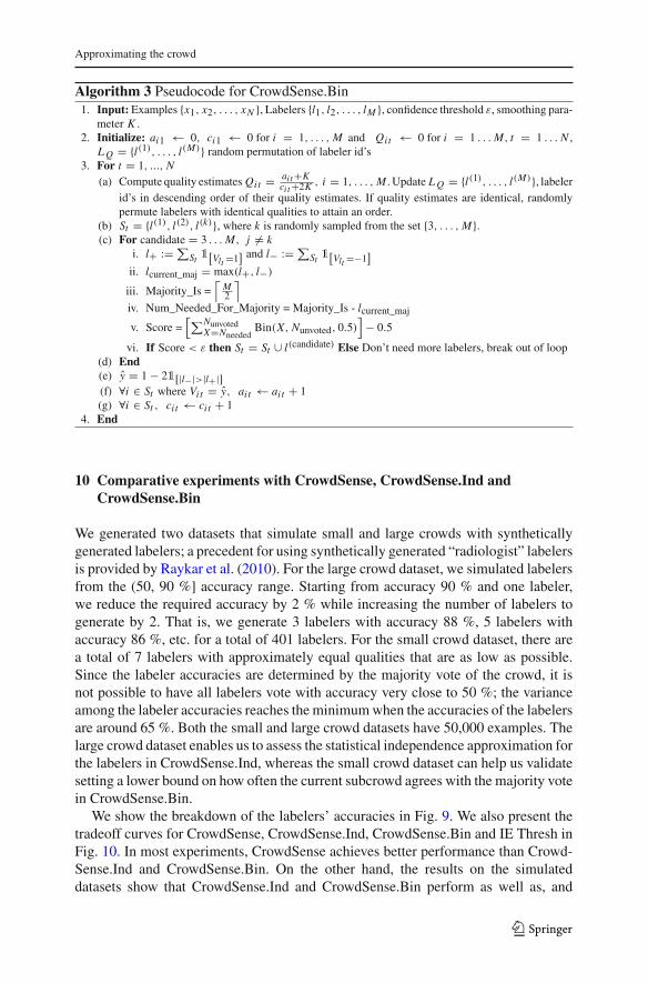
(b) St = {l(1), l(2), l(k)}, where k is randomly sampled from the set {3, . . . ,M}.(c) For candidate = 3 . . .M, j �= k

i. l+ :=∑St1[Vlt=1

] and l− :=∑St1[Vlt=−1

]ii. lcurrent_maj = max(l+, l−)

iii. Majority_Is =⌈

M2

⌉iv. Num_Needed_For_Majority = Majority_Is - lcurrent_maj

v. Score =[∑Nunvoted

X=NneededBin(X, Nunvoted, 0.5)

]− 0.5

vi. If Score < ε then St = St ∪ l(candidate) Else Don’t need more labelers, break out of loop(d) End(e) y = 1− 21[|l−|>|l+|](f) ∀i ∈ St where Vit = y, ait ← ait + 1(g) ∀i ∈ St , cit ← cit + 1

4. End

10 Comparative experiments with CrowdSense, CrowdSense.Ind andCrowdSense.Bin

We generated two datasets that simulate small and large crowds with syntheticallygenerated labelers; a precedent for using synthetically generated “radiologist” labelersis provided by Raykar et al. (2010). For the large crowd dataset, we simulated labelersfrom the (50, 90 %] accuracy range. Starting from accuracy 90 % and one labeler,we reduce the required accuracy by 2 % while increasing the number of labelers togenerate by 2. That is, we generate 3 labelers with accuracy 88 %, 5 labelers withaccuracy 86 %, etc. for a total of 401 labelers. For the small crowd dataset, there area total of 7 labelers with approximately equal qualities that are as low as possible.Since the labeler accuracies are determined by the majority vote of the crowd, it isnot possible to have all labelers vote with accuracy very close to 50 %; the varianceamong the labeler accuracies reaches the minimum when the accuracies of the labelersare around 65 %. Both the small and large crowd datasets have 50,000 examples. Thelarge crowd dataset enables us to assess the statistical independence approximation forthe labelers in CrowdSense.Ind, whereas the small crowd dataset can help us validatesetting a lower bound on how often the current subcrowd agrees with the majority votein CrowdSense.Bin.

We show the breakdown of the labelers’ accuracies in Fig. 9. We also present thetradeoff curves for CrowdSense, CrowdSense.Ind, CrowdSense.Bin and IE Thresh inFig. 10. In most experiments, CrowdSense achieves better performance than Crowd-Sense.Ind and CrowdSense.Bin. On the other hand, the results on the simulateddatasets show that CrowdSense.Ind and CrowdSense.Bin perform as well as, and

123

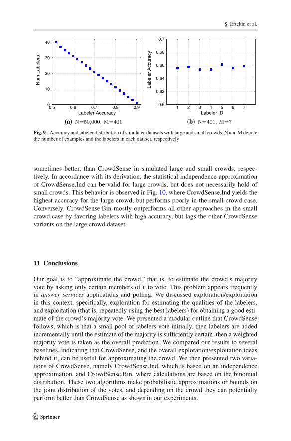
S. Ertekin et al.

0.5 0.6 0.7 0.8 0.90

10

20

30

40

Labeler Accuracy

Num

Lab

eler

s

(a) N=50,000, M=401

1 2 3 4 5 6 70.6

0.62

0.64

0.66

0.68

0.7

Labeler ID

Labe

ler

Acc

urac

y

(b) N=401, M=7

Fig. 9 Accuracy and labeler distribution of simulated datasets with large and small crowds. N and M denotethe number of examples and the labelers in each dataset, respectively

sometimes better, than CrowdSense in simulated large and small crowds, respec-tively. In accordance with its derivation, the statistical independence approximationof CrowdSense.Ind can be valid for large crowds, but does not necessarily hold ofsmall crowds. This behavior is observed in Fig. 10, where CrowdSense.Ind yields thehighest accuracy for the large crowd, but performs poorly in the small crowd case.Conversely, CrowdSense.Bin mostly outperforms all other approaches in the smallcrowd case by favoring labelers with high accuracy, but lags the other CrowdSensevariants on the large crowd dataset.

11 Conclusions

Our goal is to “approximate the crowd,” that is, to estimate the crowd’s majorityvote by asking only certain members of it to vote. This problem appears frequentlyin answer services applications and polling. We discussed exploration/exploitationin this context, specifically, exploration for estimating the qualities of the labelers,and exploitation (that is, repeatedly using the best labelers) for obtaining a good esti-mate of the crowd’s majority vote. We presented a modular outline that CrowdSensefollows, which is that a small pool of labelers vote initially, then labelers are addedincrementally until the estimate of the majority is sufficiently certain, then a weightedmajority vote is taken as the overall prediction. We compared our results to severalbaselines, indicating that CrowdSense, and the overall exploration/exploitation ideasbehind it, can be useful for approximating the crowd. We then presented two varia-tions of CrowdSense, namely CrowdSense.Ind, which is based on an independenceapproximation, and CrowdSense.Bin, where calculations are based on the binomialdistribution. These two algorithms make probabilistic approximations or bounds onthe joint distribution of the votes, and depending on the crowd they can potentiallyperform better than CrowdSense as shown in our experiments.

123

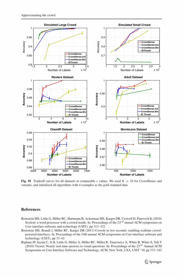
Approximating the crowd

1.5 2 2.5 3 3.5x 10

5

0.8

0.85

0.9

0.95

1Simulated Large Crowd

Number of Labels

Acc

urac

y

CrowdSenseCrowdSense.IndCrowdSense.BinIEThresh

1 1.5 2 2.5 3 3.5 4x 10

5

0.7

0.8

0.9

1Simulated Small Crowd

Number of Labels

Acc

urac

y CrowdSenseCrowdSense.IndCrowdSense.BinIEThresh

2 4 6 8 10x 10

4

0.92

0.94

0.96

0.98

1Reuters Dataset

Number of Labels

Acc

ura

cy

CrowdSenseCrowdSense.IndCrowdSense.BinIE Thresh

0 1 2 3 4 5x 10

5

0.9

0.95

1Adult Dataset

Number of Labels

Acc

ura

cy

CrowdSenseCrowdSense.IndCrowdSense.BinIE Thresh

2000 3000 4000 5000 6000 70000.86

0.88

0.9

0.92

0.94

0.96ChemIR Dataset

Number of Labels

Acc

ura

cy

CrowdSenseCrowdSense.IndCrowdSense.BinIE Thresh

500 1000 1500

0.96

0.97

0.98

0.99

1MovieLens Dataset

Number of Labels

Acc

ura

cy

CrowdSenseCrowdSense.IndCrowdSense.BinIE Thresh

Fig. 10 Tradeoff curves for all datasets at comparable ε values. We used K = 10 for CrowdSense andvariants, and initialized all algorithms with 4 examples as the gold standard data

References

Bernstein MS, Little G, Miller RC, Hartmann B, Ackerman MS, Karger DR, Crowell D, Panovich K (2010)Soylent: a word processor with a crowd inside. In: Proceedings of the 23rd annual ACM symposium onUser interface software and technology (UIST), pp 313–322

Bernstein MS, Brandt J, Miller RC, Karger DR (2011) Crowds in two seconds: enabling realtime crowd-powered interfaces. In: Proceedings of the 24th annual ACM symposium on User interface software andtechnology (UIST), pp 33–42

Bigham JP, Jayant C, Ji H, Little G, Miller A, Miller RC, Miller R, Tatarowicz A, White B, White S, Yeh T(2010) Vizwiz: Nearly real-time answers to visual questions. In: Proceedings of the 23rd Annual ACMSymposium on User Interface Software and Technology, ACM, New York, USA, UIST ’10, pp 333–342

123

S. Ertekin et al.

Callison-Burch C, Dredze M (2010) Creating speech and language data with amazon’s mechanical turk. In:Proceedings of the NAACL HLT 2010 Workshop on Creating Speech and Language Data with Amazon’sMechanical Turk, pp 1–12

Dakka W, Ipeirotis PG (2008) Automatic extraction of useful facet hierarchies from text databases. In:Proceedings of the 24th International Conference on Data Engineering (ICDE), pp 466–475

Dawid AP, Skene AM (1979) Maximum likelihood estimation of observer error-rates using the em algorithm.Appl. Stat. 28(1):20–28

Dekel O, Shamir O (2009a) Good learners for evil teachers. In: Proceedings of the 26th Annual InternationalConference on Machine Learning (ICML)

Dekel O, Shamir O (2009b) Vox populi: Collecting high-quality labels from a crowd. In: Proceedings ofthe 22nd Annual Conference on Learning Theory

Dekel O, Gentile C, Sridharan K (2010) Robust selective sampling from single and multiple teachers. In:The 23rd Conference on Learning Theory (COLT), pp 346–358

Donmez P, Carbonell JG, Schneider J (2009) Efficiently learning the accuracy of labeling sources forselective sampling. In: Proceedings of the 15th International Conference on Knowledge Discovery andData Mining (KDD), pp 259–268

Downs JS, Holbrook MB, Sheng S, Cranor LF (2010) Are your participants gaming the system?: screeningmechanical turk workers. In: Proceedings of the 28th international conference on Human factors incomputing systems, CHI ’10, pp 2399–2402

Ertekin S, Hirsh H, Rudin C (2012) Learning to predict the wisdom of crowds. In: Proceedings of CollectiveIntelligence, CI’12, Cambridge, Massachusetts

Gillick D, Liu Y (2010) Non-expert evaluation of summarization systems is risky. In: Proceedings of theNAACL HLT 2010 Workshop on Creating Speech and Language Data with Amazon’s Mechanical Turk,Association for Computational Linguistics, CSLDAMT ’10, pp 148–151

Hsueh PY, Melville P, Sindhwani V (2009) Data quality from crowdsourcing: a study of annotation selectioncriteria. In: Proceedings of the NAACL HLT 2009 Workshop on Active Learning for Natural LanguageProcessing, pp 27–35

Ipeirotis PG, Provost F, Wang J (2010) Quality management on amazon mechanical turk. In: Proceedingsof the ACM SIGKDD Workshop on Human Computation, ACM, New York, USA, HCOMP ’10, pp64–67

Ipeirotis PG, Provost F, Sheng VS, Wang J (2013) Repeated labeling using multiple noisy labelers. DataMin Knowl Discov 28(2):402–441

Kaisser M, Lowe J (2008) Creating a research collection of question answer sentence pairs with ama-zons mechanical turk. In: Proceedings of the 6th International Language Resources and Evaluation(LREC’08), European Language Resources Association (ELRA)

Kasneci G, Gael JV, Stern D, Graepel T (2011) Cobayes: bayesian knowledge corroboration with assessorsof unknown areas of expertise. In: Proceedings of the 4th ACM International Conference on Web Searchand Data Mining (WSDM), pp 465–474

Law E, von Ahn L (2011) Human computation, synthesis lectures on artificial intelligence and machinelearning. Morgan & Claypool Publishers, San Rafael

Marge M, Banerjee S, Rudnicky A (2010) Using the amazon mechanical turk for transcription of spokenlanguage. In: Acoustics Speech and Signal Processing (ICASSP), 2010 IEEE International Conferenceon, pp 5270–5273

Mason W, Watts DJ (2009) Financial incentives and the “performance of crowds”. In: Proceedings of theACM SIGKDD Workshop on Human Computation, HCOMP ’09, pp 77–85

Nakov P (2008) Noun compound interpretation using paraphrasing verbs: Feasibility study. In: Proceedingsof the 13th international conference on Artificial Intelligence: Methodology, Systems, and Applications,Springer-Verlag, Berlin, Heidelberg, AIMSA ’08, pp 103–117

Nowak S, Rüger S (2010) How reliable are annotations via crowdsourcing: a study about inter-annotatoragreement for multi-label image annotation. In: Proceedings of the international conference on Multi-media information retrieval, MIR ’10, pp 557–566

Ogawa S, Piller F (2006) Reducing the risks of new product development. MITSloan Manag Rev 47(2):65Quinn AJ, Bederson BB (2011), Human computation: a survey and taxonomy of a growing field. In:

Proceedings of the 2011 Conference on Human Factors in, Computing Systems, pp 1403–1412Raykar VC, Yu S, Zhao LH, Valadez GH, Florin C, Bogoni L, Moy L (2010) Learning from crowds. J Mach

Learn Res (JMLR) 11:1297–1322

123

Approximating the crowd

Sheng VS, Provost F, Ipeirotis PG (2008) Get another label? improving data quality and data mining usingmultiple, noisy labelers. In: Proceeding of the 14th International Conference on Knowledge Discoveryand Data Mining (KDD), pp 614–622

Smyth P, Burl MC, Fayyad UM, Perona P (1994a) Knowledge discovery in large image databases: Dealingwith uncertainties in ground truth. In: KDD, Workshop, pp 109–120

Smyth P, Fayyad UM, Burl MC, Perona P, Baldi P (1994b) Inferring ground truth from subjective labellingof venus images. In: NIPS, pp 1085–1092

Snow R, O’Connor B, Jurafsky D, Ng AY (2008) Cheap and fast–but is it good?: evaluating non-expertannotations for natural language tasks. In: Proceedings of the Conference on Empirical Methods inNatural Language Processing (EMNLP), pp 254–263

Sorokin A, Forsyth D (2008) Utility data annotation with amazon mechanical turk. Computer Vision andPattern Recognition Workshop 1–8

Sullivan EA (2010) A group effort: more companies are turning to the wisdom of the crowd to find waysto innovate. Mark News 44(2):22–28

Wallace BC, Small K, Brodley CE, Trikalinos TA (2011) Who should label what? instance allocation inmultiple expert active learning. In: Proceedings of the SIAM International Conference on Data Mining(SDM)

Warfield SK, Zou KH, Wells WM (2004) Simultaneous truth and performance level estimation (staple): analgorithm for the validation of image segmentation. IEEE Transact Med Imaging (TMI) 23(7):21–903

Welinder P, Branson S, Belongie S, Perona P (2010) The multidimensional wisdom of crowds. In: Advancesin Neural Information Processing Systems (NIPS) vol 10, pp 2424-2432

Whitehill J, Ruvolo P, fan Wu T, Bergsma J, Movellan J (2009) Whose vote should count more: Optimalintegration of labels from labelers of unknown expertise. In: Advances in Neural Information ProcessingSystems (NIPS), pp 2035–2043

Yan Y, Rosales R, Fung G, Dy J (2010b) Modeling multiple annotator expertise in the semi-supervisedlearning scenario. In: Proc. of the 26th Conference on Uncertainty in Artificial Intelligence (UAI),AUAI Press, Corvallis, Oregon, pp 674–682

Yan Y, Rosales R, Fung G, Schmidt MW, Valadez GH, Bogoni L, Moy L, Dy JG (2010b) Modeling annotatorexpertise: Learning when everybody knows a bit of something. J Mac Learn Res-Proc Track 9:932–939

Zheng Y, Scott S, Deng K (2010) Active learning from multiple noisy labelers with varied costs. In: 10thIEEE International Conference on Data Mining (ICDM), pp 639–648

123