Settore Concorsuale di afferenza: 08/A1 Settore ...amsdottorato.unibo.it/6626/1/raosa_andrea_natalia_tesi.pdf · 7 Figure 4.13. Wave height trend on the dike crest for tests characterized

1

Alma Mater Studiorum – Università di Bologna

DOTTORATO DI RICERCA IN

INGEGNERIA CIVILE E AMBIENTALE

Ciclo XXVI

Settore Concorsuale di afferenza: 08/A1

Settore Scientifico disciplinare: ICAR/01

ANALYSIS AND MATHEMATICAL MODELING

OF WAVE-STRUCTURE INTERACTION

Presentata da:

Andrea Natalia Raosa

Coordinatore Dottorato Relatore

Chiar.mo Prof. Alberto Lamberti Prof. Barbara Zanuttigh

Relatore

Prof. Javier L. Lara

Esame finale anno 2013-2014

2

Index

List of figures ..................................................................................................................... 5

List of tables ..................................................................................................................... 12

Chapter 1 INTRODUCTION ........................................................................................ 14

1.1 Motivations ............................................................................................................ 14

1.2 Background ............................................................................................................ 15

1.3 Definition of the objectives .................................................................................... 17

1.4 Outline .................................................................................................................... 18

Chapter 2 SEDIMENT TRANSPORT MODELLING IN THE SWASH ZONE. STATE OF

THE ART. ........................................................................................................................ 19

2.1 Parametric and empirical modeling of cross-shore swash zone sediment transport20

2.2 Longshore sediment transport rate (LSTR) ............................................................ 23

2.3 Process-based numerical modeling of swash zone sediment transport .................. 26

2.3.1 Non-linear shallow water equations (NLSWE) ............................................... 26

2.3.2 Boussinesq equations ...................................................................................... 29

2.3.3 Navier-Stokes equations (NSE) ...................................................................... 32

Chapter 3 THE IH-2VOF NUMERICAL MODEL. ................................................... 40

3.1 Governing equations in the fluid domain: the Reynolds Averaged Navier-Stokes (RANS)

equations ....................................................................................................................... 41

3.2 Initial and boundary conditions .............................................................................. 45

3.2.1 Initial conditions .............................................................................................. 45

3.2.2 Boundary conditions ....................................................................................... 46

3.3 Free surface tracking trough the volume of fluid (VOF) method .......................... 49

3.4 Partial cell treatment............................................................................................... 50

3.5 Governing equations for the flow in porous media (VARANS equations) ............ 50

3.6 Schematics of computational domain .................................................................... 57

3

3.7 Numerical resolution .............................................................................................. 59

3.8 Resolution procedure.............................................................................................. 61

Chapter 4 REPRESENTATION OF THE WAVE OVERTOPPING PROCESS. .. 62

4.1 Design criteria for coastal defences structures ....................................................... 63

4.2 Overtopping over a seadikes .................................................................................. 66

4.2.1 Wave overtopping discharge ........................................................................... 66

4.2.2 Overtopping flow velocities and overtopping flow depth ............................... 70

4.3 The numerical database .......................................................................................... 73

4.4 Validation of the model .......................................................................................... 74

4.4.1 Wave reflection coefficient ............................................................................. 75

4.4.2 Overtopping discharge .................................................................................... 77

4.5 Flow height evolution over the dike crest .............................................................. 80

4.5.1 Influence of the dike submergence and geometry ........................................... 80

4.5.2 Comparison with the theory ............................................................................ 83

4.5.3 Formula for the determination of the decay coefficient .................................. 89

4.6 Flow velocity evolution over the dike crest ........................................................... 91

4.6.1 Influence of the dike submergence and geometry ........................................... 91

4.6.2 Approximation of the velocity trend with a fitting function ........................... 94

4.7 Statistical characterization of extreme overtopping wave volumes ..................... 100

Chapter 5 TWO-PHASE APPROACH FOR SEDIMENT TRANSPORT MODELLING. 103

5.1 Governing equations for fluid and particle phase: RANS equations ................... 103

5.2 Closure of fluid stresses ....................................................................................... 106

5.3 Closure of sediment stresses ................................................................................ 110

5.4 Model implementation ......................................................................................... 117

5.5 Spatial discretization in finite different form ....................................................... 120

5.5.1 Advection terms ............................................................................................ 122

4

5.5.2 New advection terms ..................................................................................... 125

5.5.3 Tangential terms ............................................................................................ 127

5.5.4 Drag force terms ............................................................................................ 132

5.5.5 Pressure terms ............................................................................................... 133

Chapter 6 WAVE-INDUCED EROSION AND DEPOSITION PATTERNS: VERIFICATION

OF MODEL RESULTS. ............................................................................................... 136

6.1 Computational set-up ........................................................................................... 136

6.2 Results for test P1 ................................................................................................. 137

6.3 Results for test P2 ................................................................................................. 142

Chapter 7 CONCLUSIONS AND FUTURE WORK. .............................................. 146

REFERENCES .............................................................................................................. 150

5

LIST OF FIGURES

Figure 2.1. Schematic illustration of swash zone (Elfrink and Baldock, 2002).

……………………………………………………………………………………………………….19

Figure 3.1. Schematics of computational domain with the different cell types on the

information of the VOF function and definition of the computed magnitudes.

……………………………………………………………………………………………………….58

Figure 3.2. Schematics of solid boundaries definition through the partial cell treatment.

……………………………………………………………………………………………………….58

Figure 4.1. Severe wave overtopping at the Samphire Hoe seawall, UK (CLASH project,

www.clash-eu.org, 2001).

……………………………………………………………………………………………………….62

Figure 4.2. Wave overtopping and overflow for positive, zero and negative freeboard (by

Eurotop 2007).

……………………………………………………………………………………………………….68

Figure 4.3. Definition sketch for overtopping flow parameters on the dike crest (by

Eurotop 2007).

……………………………………………………………………………………………………….71

Figure 4.4. Overtopping flow velocity data vs overtopping flow velocity formulae (by

Eurotop 2007).

……………………………………………………………………………………………………….72

Figure 4.5. Left side: influence of overtopping flow depth on overtopping flow velocity;

right side: influence of bottom friction on overtopping flow velocity (by Eurotop 2007).

……………………………………………………………………………………………………….72

http://www.clash-eu.org/

6

Figure 4.6. Tested levee cross section (model-scale units).

……………………………………………………………………………………………………….74

Figure 4.7. obtained by the experimental database for smooth straight (Zanuttigh and

Van der Meer, 2006) and the numerical simulation characterized by and

.

……………………………………………………………………………………………………….75



.

……………………………………………………………………………………………………….76



.

……………………………………………………………………………………………………….76

Figure 4.10. Total numerical discharge versus total theoretical discharge for

emerged cases.

……………………………………………………………………………………………………….78

Figure 4.11. Total numerical discharge versus total theoretical discharge for

cases with zero freeboard.

……………………………………………………………………………………………………….78

Figure 4.12. Wave height trend on the dike crest for test T17C ( , red), T9B

( , blue), T1A ( , green), and T25D ( , yellow).

……………………………………………………………………………………………………….82

7

Figure 4.13. Wave height trend on the dike crest for tests characterized by landward

slope 1:3 (circles) and 1:2 (crosses) and different freeboard.

……………………………………………………………………………………………………….82

Figure 4.14. Wave height trend on the dike crest for tests characterized by seaward slope

1:4 (circles) and 1:6 (crosses) and different freeboard.

……………………………………………………………………………………………………….83

Figure 4.15. Wave height decay on the dike crest with and .

Squares: cases with and ; triangles: cases with and

; diamonds: cases with and .

……………………………………………………………………………………………………….86




……………………………………………………………………………………………………….86




……………………………………………………………………………………………………….87




……………………………………………………………………………………………………….87

8




……………………………………………………………………………………………………….88




……………………………………………………………………………………………………….88

Figure 4.21. Wave decay coefficients against new Equation 4.14. Tests with

.

……………………………………………………………………………………………………….90

Figure 4.22. Wave decay coefficients against new Equation 4.14. Tests with .

……………………………………………………………………………………………………….90

Figure 4.23. Wave decay coefficients against new Equation 4.14. Tests with

.

……………………………………………………………………………………………………….91

Figure 4.24. Flow velocity trend on the dike crest for test T17C (Rc/Hs=0.5, red), T9B

( , blue), T1A ( , green), and T25D ( , yellow).

……………………………………………………………………………………………………….92

Figure 4.25. Flow velocity trend on the dike crest for tests characterized by landward


……………………………………………………………………………………………………….93

Figure 4.26. Flow velocity trend on the dike crest for tests characterized by seaward


……………………………………………………………………………………………………….93

9

Figure 4.27. Wave velocity evolution on the crest of the structure for tests with

and . Squares: cases with and ; triangles:

cases with and ; diamonds: cases with and

.

……………………………………………………………………………………………………….95




.

……………………………………………………………………………………………………….95


and . Squares: cases with and ; triangles: cases

with and ; diamonds: cases with and .

……………………………………………………………………………………………………….96


and . Squares: cases with and ; triangles: cases

with and ; diamonds: cases with and .

……………………………………………………………………………………………………….96




.

……………………………………………………………………………………………………….97

10




.

……………………………………………………………………………………………………….97

Figure 4.33. Comparison numerical results ( ) with smooth structures

against formula 4.16.

……………………………………………………………………………………………………101

Figure 4.34. Comparison numerical results ( , orange; , green;

, pink; , blue) with smooth structures against formula 4.16.

…………………………………………………………………………………………………….102

Figure 6.1. Sketch of the cases tested.

…………………………………………………………………………………………………….137

Figure 6.2. Water depth trend measured at from the beginning of the channel.

…………………………………………………………………………………………………….137

Figure 6.3. Water depth trend along the channel at (red), (green) and

(blue).

…………………………………………………………………………………………………….138

Figure 6.4. Bottom level along the channel at (red), (green) and

(blue).

…………………………………………………………………………………………………….138

Figure 6.5. Horizontal velocity at the gauge sets at from the begin of the

channel.

…………………………………………………………………………………………………….139

11

Figure 6.6. Horizontal velocity at the gauge sets at from the begin of the

channel.

…………………………………………………………………………………………………….139

Figure 6.7. Sediment concentration at the gauge sets at x=1 m from the begin of the

channel.

…………………………………………………………………………………………………….140

Figure 6.8. Sediment concentration at the gauge sets at x=8 m from the begin of the

channel.

…………………………………………………………………………………………………….141

Figure 6.9. Water depth trend along the channel at t = 20 s (red), t = 50 s (green) and

t = 80 s (blue).

…………………………………………………………………………………………………….142

Figure 6.10. Bottom level along the channel at t = 20 s (red), t = 50 s (green) and

t = 80 s (blue).

…………………………………………………………………………………………………….142

Figure 6.11. Sediment concentration at the gauge sets at from the begin of the

channel.

…………………………………………………………………………………………………….143


channel.

…………………………………………………………………………………………………….144


channel.

…………………………………………………………………………………………………….144

12

LIST OF TABLES

Table 4.1. Characteristics of simulated tests.

……………………………………………………………………………………………………….73

Table 4.2. Model settings adopted for the numerical simulations.

……………………………………………………………………………………………………….74


……………………………………………………………………………………………………….77


……………………………………………………………………………………………………….77


……………………………………………………………………………………………………….79

Table 4.6. Flow characteristics at the dike off-shore edge ( ).

……………………………………………………………………………………………………….81

Table 4.7. Wave decay coefficients of the best fitting and relative standard deviation.

……………………………………………………………………………………………………….84

Table 4.8. Average wave decay coefficients and relative standard deviation for each

tests.

……………………………………………………………………………………………………….85

Table 4.9. Coefficients obtained with the best fitting curve for the wave velocity on the

dike crest and relative standard deviation.

……………………………………………………………………………………………………….98

13

Table 4.10. Average coefficients for wave velocity evolution on the dike crest and relative

standard deviation for each tests.

……………………………………………………………………………………………………….99

Table 6.1. Characteristics of cases tested.

…………………………………………………………………………………………………...…136

CHAPTER 1

INTRODUCTION

1.1 Motivations

Shore protection against erosion has turned to be a major issue in a great part of the

worldwide coastal areas. About 80% of the world shorelines are under an erosion process

while 70% of the global human population, representing 4 billions of persons, live in a 60

km-wide strip contiguous to the sea. The natural tendency of coastal erosion has been

dramatically accelerated by the impact of human activities, and the average rate of

shoreline recession in some coastal sites of the world reaches values of tens of meters a

year (Komar, 1998; Pilkey and Hume, 2001). In particular, in the countries of the

European Union, about 20.000 km of coasts, i.e. 20% of the European coasts, are to some

extent affected by erosion, being most of them actively retreating. The area lost or

seriously impacted by erosion is estimated to be 15 km2

per year. Extensive coastal areas

in the Netherlands, England, Germany, Poland and Italy are already at an altitude lower

than the levels of the high tide and therefore inherently more vulnerable to flooding. At

the same time, over the past 50 years, the population living in European coastal

municipalities has more than doubled to reach 70 millions inhabitants in 2001

(EUROSION UE project).

Hence, the population and development pressures on the coastal zones require life and

property defense policies from coastal hazards and the definition of technical alternatives

for shore protection. The response options to eroding coasts are multifold, and have been

basically split into “soft” solutions, mainly beach nourishment designs, and “hard”

solutions of shoreline stabilization using seawalls, grayness and offshore breakwaters.

Climate change will have significant impacts on coastal areas, due to the sea level rise

(based on the SRES scenarios in the range 0.2-0.8 m/century) and the increased frequency

Chapter 1

15

and intensity of extreme events. So, the large stretches of the coast that are protected by

hard structures, are very sensitive to rising average sea level because these kind of

structures will be more frequently overflowed and the shoreline will consequently subject

to greater wave energy remaining. These elements make essential an accurate knowledge

of the phenomena of wave-structure interaction and the rising wave on the beach and / or

dunes which over time can be eroded until the formation of a breach.

The University of Bologna has leaded the investigation tasks of the THESEUS project

and the present PhD Thesis has been realised in the frame of this project. One of the

main objectives of the project was to analyse innovative technologies aimed at the

mitigation of the flood and erosion risk (as resilient dikes or over-washed structures).

The increase of frequency and intensity of storms, combined with the uncertainties related

to extreme events and climate change, carries an increased the risk of flooding of low

lying areas, an accelerate erosion of exposed soft beaches and a challenges in the long

term design of coastal protection structures. The aim of this thesis work, included within

the THESEUS project, is the development of a mathematical model 2DV two-phase,

based on an existing code, able to represent the real conditions of inundation i.e able to

represent together the overtopping phenomenon on emerged/submerged structures and the

sediment transport.

1.2 Background

Traditionally wave-structure interaction has been studied through physical tests (two- and

three-dimensional, small- and large- scale model tests). Empirical formulations arisen

from physical modeling present several restrictions and a narrow range of applicability.

Many other issues related with scale factors or processes such as porous media flow,

wave impacts or viscous effects are not correctly represented in the experiments. A great

effort has been made over the last decade in the numerical modeling of wave interaction

with coastal structures to overcome these limitations.

Chapter 1

16

A similar consideration can be made also for the study of the sediment transport. In fact,

field experimentation is challenging due to the difficulty and expense in deploying

equipment, obtaining robust data and the variability of meteorological conditions.

Although, laboratory measurements have some limitations, due to the constrained

circumstances compared with the field, the data obtained are the most reliable for

investigating processes and for validating models. Meanwhile, developments in

computational hardware and numerical solution methods have driven the popularity of

numerical modeling of coastal hydrodynamics.

Several approaches have been followed to study the wave-structure interaction, the

induced hydrodynamic and the consequently mixing and sediment suspension. Among

other existing approaches, Nonlinear Shallow Water (NSW), Boussinesq-type or Navier-

Stokes equations models have traditionally been used.

Good results in terms of averaged magnitudes have been obtained using NSW equation

(Kobayashi et al., 2007), though vertical velocity structure cannot be resolved using this

approach and the energy transfer to higher frequencies occurring before wave breaking

cannot be reproduced accurately due to the lack of dispersion.

Boussinesq-type models are able to include frequency dispersion, a depth-dependent

velocity profile, and they can be applied to both breaking and non-breaking wave

conditions. A great effort has been made in order to relax the original equations by

deriving the extended Boussinesq equations (Kirby, 2003). However, this type of models

requires setting both the triggering wave breaking mechanism and the subsequent wave

energy dissipation due to wave breaking. Moreover, these models fail to reproduce the

strong nonlinear shoaling prior to wave breaking and the free-surface and velocity higher

order statistics which are thought to be relevant for structure stability.

Navier-Stokes equations models assume a number of simplifications in the equations

lower than in other approaches. These models are able to calculate flows in complex

geometries and provide very refined information on the velocity, pressure and turbulence

field. Models based on a two dimensional eulerian Navier-Stokes set of equations

(Losada et al., 2008; Lara et al., 2008; Guanche et al., 2009; Lara et al., 2011) have

proven to be powerful to address wave-induced processes. Wave reflection and

Chapter 1

17

overtopping have been reproduced numerically with a high degree of accuracy,

introducing new models to be used as a complementary tool in the design process. These

types of models are so accurate and promising that 3D applications were developed (P.

Higuera et al., 2013).

Wave-structure interaction and wave run-up on beaches and/or dunes require models

capable to deal with steep and emerged slopes. Traditional 2DH numerical models, such

as Mike21 Shallow Water equations model (SW+HD modules), can be applied only when

the structure/beach is submerged. Other models, such as the Boussinesq models (as Mike

21 BW module) can be powerful tools for run-up and overtopping in case of steep slopes

up to 1:3 but so far are time consuming tools (high spatial resolution, low Courant

number) and need the introduction of a lot of artificial dissipation usually to avoid

instabilities: application thus depends on the extension of the area to be modelled and on

the phenomena to be included (wave breaking, wave run-up). Moreover, existing

Boussinesq models do not include the representation of sediment transport do that

beach/dune reshaping during storms and possible breaching cannot be reproduced. So far

only RANS-VOF models can deal with wave run-up and overtopping on steep slopes

(also structures, slopes 1:2) without the inclusion of many artifices.

1.3 Definition of the objectives

The overall aim of this thesis is to develop a tool that can represent wave run-up and

overtopping together with beach reshaping during storms. Actually what can be a more

promising research field, due to the lack of good representation for many of the related

processes, is the modellisation of the swash zone that is an area of greatest importance

both for flooding issues and ecosystem conservation.

The specific objectives of the present study are:

to characterize the flow (velocities and layer thicknesses) on the crest of the

structure in order to extend the theoretical models and provide criteria for the

design of structures close to mean sea level or overwashed;

Chapter 1

18

to introduce in a two-dimensional numerical model based on the Reynolds

Averaged Navier–Stokes equations (RANS), called IH-2VOF (Losada et al.,

2008), new equations for the representation of the sediment transport;

to verify the model as a reliable tool for the simulation of wave-structures

interactions and sediment transport dynamics.

1.4 Outline

The present thesis is organized following the objectives listed above.

In chapter 1, an introductive description of the work and the objectives of the study are

presented.

In chapter 2, a state-of-the-art review of both experimental and mathematical the

modelling of sediment transport is included.

In chapter 3, the characteristics of the numerical model used to carry out the present work

are described. The governing equations and main mathematical assumptions, free surface

tracking method and resolution procedure are presented.

In chapter 4, previously the existing theories for the overtopping process are described,

than the numerical tests and its set-up for the study of wave overtopping process above a

particular kind of coastal defense structure are introduced. The key results obtained by

the numerical simulation (for example the influence of the seaward-landward slope and of

the dike submergence), the analysis of the wave flow characteristics above the structure

and the comparison with the theoretical approach are reported.

In chapter 5, the modifications of the initial code are reported. New equations

implemented for the representation of the sediment transport in a two-phase model are

shown and described.

In chapter 6, the stages and results of the two-phase model verification process are

presented.

In chapter 7, conclusions and discussion are finally drawn.

CHAPTER 2

SEDIMENT TRANSPORT MODELLING IN

THE SWASH ZONE. STATE OF THE ART.

The surf and swash zones are hydrodynamically active regions. Nearshore breaking

waves play a paramount role in coastal morphology and influence most coastal processes.

These waves produce highly turbulent regions causing significant mixing and sediment

suspension. The suspended sediments are transported by the nearshore currents induced

by breaking waves. Moreover, breaking waves impact offshore structures and should be

considered in their design. Fluid and sediment interactions occurring in the swash zone

determine the erosion or accretion of a beach and act as boundary conditions for

nearshore hydrodynamic and morphodynamic models. A schematic illustration of the

surf and swash zones is shown in Figure 2.1.

Figure 2.1. Schematic illustration of swash zone (Elfrink and Baldock, 2002).

In this chapter a critical review of conceptual and mathematical models developed in

recent decades on sediment transport in the swash zone is presented.

Chapter 2

20

Evidently, the hydrodynamics of the swash zone are complex and not fully understood.

Key hydrodynamic processes include both high-frequency bores and low-frequency

infragravity motions, and are affected by wave breaking and turbulence, shear stresses

and bottom friction. The prediction of sediment transport that results from these complex

and interacting processes is a challenging task. Besides, sediment transport in this

oscillatory environment is affected by high-order processes such as the beach ground

water flow. Most relationships between sediment transport and flow characteristics are

empirical, based on laboratory experiments and/or field measurements. Analytical

solutions incorporating key factors such as sediment characteristics and concentration,

waves and coastal aquifer interactions are unavailable. Therefore, numerical models for

wave and sediment transport are widely used by coastal engineers.

2.1 Parametric and empirical modeling of cross-shore swash zone

sediment transport

The swash zone sediment transport and foreshore evolution have been analyzed in several

studies (e.g., Masselink et al., 2005; Miles et al., 2006). Empirical formulas based on

numerous experiments on steady flow have been implemented to describe the amount of

sediment transport (Nielsen, 1990). Most of these formulas were based on the

relationship between the Shields parameter (Shields, 1936) and the dimensionless

sediment transport rate.

Madsen (1991) derived a sediment transport rate formula for the instantaneous bed-load

that was further generalized by Madsen (1993). Masselink and Hughes (1998)

found that Bagnold’s energetics-based bed-load sediment transport equations fitted their

field data, and concluded that formulae based on a modified Shields parameter could also

be used. Since physically the up-rush and back wash flows are different, it seems logical

that the associated sediment transport processes can also be different. Masselink and

Hughes (1998) showed that swash zone sediment transport rate formula required different

empirical constants ( ) in order to fit measured velocities and sediment transport rates in

both up-rush and back wash phases of the swash.

Chapter 2

21

On one hand, the modeling approach using two different values of model coefficient is

consistent with differences between the up wash and back wash (flow characteristics and

sediment transport modes) as speculated by previous researchers (Nielsen, 2002). On the

other hand, our limited understanding of the up wash and back wash hydrodynamics

prevents us from quantifying further these coefficients for different conditions (different

values have been obtained for different data sets; i.e., they remain empirical). Nielsen

(2002) presented two mechanisms for the sediment transport during up-rush:‘‘(i) the

existence of higher shear stresses during up-rush; and (ii) the existence of pre-floating

sediment from the bore collapse (Masselink and Hughes, 1998)’’. The shear stress of the

bed was modeled by the time series of the free stream velocity in terms of the wave

boundary layer model plus a phase lead of the bed shear stress, compared with the

free stream velocity at the peak frequency. He postulated that the total amount of

sediment transport during up-rush and back wash is well estimated by the model without

the need for incorporating different multipliers for up-rush and back wash and suggested

that the range in values is 9.7 0.2 (Nielsen,2002). It should be noted that although the

total amount of sediment transport is the same, the timing of sediment transport rate has

not yet been accurately modeled due to the very unsteady nature of the swash zone and

the existence of pre-floated sediments. Besides, some mechanisms have not been

considered in this formulation. For example, the observed lag between the instantaneous

bed shear stress and the rate of sediment transport has not been considered

(Nielsen,2002).

Larson et al. (2004) developed the sediment transport formulae to predict the net transport

rate over many swash cycles and compared the predictions with field data. Net sediment

transport rate sand the formulae developed to calculate the net sediment transport in the

swash zone showed good agreement with transport rate measurements at the seaward end

of the swash.

Drake and Calantoni (2001) added an extra term to the Bailard formula to account for

acceleration effects and showed that the inclusion of acceleration effects improved the

performance of the transport model. Puleo et al. (2003) also modified an energetics

model for sediment transport to include the effect of fluid acceleration and were able to

Chapter 2

22

strongly reduce the prediction error. Pedrozo-Acuña et al. (2007) modified the bed-load

formulation to include an acceleration term similar to that proposed by Drake and

Calantoni (2001):

{

| |

(2.1)

where is the Shields parameter; is the local beach angle; is the friction angle for a

moving grain; is the horizontal velocity at the sea floor; is the acceleration

threshold and is the efficiency. The acceleration is calculated by differentiating the

velocity time series from the hydrodynamic model. The addition of an acceleration term

does not by itself improve the prediction. However, it enables morphological models to

predict on shore migration of bars, in accordance with results shown by previous

researchers (Pedrozo-Acuña etal., 2007).

Karambas (2003,2006) derived the non-dimensional sediment transport rate based on

modified Meyer-Peterand Muller (1948) formula using different values the multiplier

for up-rush and back wash that includes infiltration/exfiltration effects.

Note that a Shields-type transport formula does not account for inertial forces, which may

become significant for coarse grains due to the high fluid accelerations during up wash

(Baldock and Holmes, 1997). In summary, none of the above models can resolve all

potentially important details of the flow and sediment transport in the swash zone, such as

the wave boundary layer, percolation, flow separation at the beach step and the 2D or 3D

distribution of suspended sediments. Despite these efforts, the energetics-based models

are unable to account for the phase difference between the sediment transport rate and

hydrodynamic forcing parameters. Hsu and Raubenheimer (2006) indicated that

sediment transport in the swash zone might not correlate to the instantaneous forcing

computed in a specific location, so such equations might not be valid in the swash. A

means to make progress on this issue are process-based and a two-phase modeling

approach.

Chapter 2

23

2.2 Longshore sediment transport rate (LSTR)

The longshore current generated by obliquely incident breaking waves plays an important

role in transporting sediment in the swash zone and is a key component of most coastal

engineering studies (Kumar et al.,2003). Under obliquely incident waves, near shore

sediment moves in a zig-zag way that results in LST in the swash zone (Asano, 1994).

The cross-shore distributions of LST indicate three distinct zones of transport: the

incipient breaker zone, the inner surf zone and the swash zone (Smith et al., 2004). A

peak in transport occurs for plunging waves in the incipient breaker zone, indicating that

this breaker type suspends more sediment for transport. The breaker is a function of

wave height, period and beach slope. In the inner surf zone, wave height is the

dominating factor in controlling sediment transport, which depends less on wave period.

Swash zone sediment transport, which accounts for a significant percentage of the total

transport, shows a dependence on wave height, period and beach slope. The occurrence

of the increased longshore flow velocities in the swash zone is related to differences in

fluid motion between the inner surf zone and swash zone (Smith et al., 2004).

In the surf zone, the oscillatory part of the flow is directed more or less perpendicular to

the wave crests. In the swash zone, however, the flow direction during up-rush is

perpendicular to the wave crest, but perpendicular to the beach orientation during

backwash, in the absence of longshore current. This effect increases with increasing bed

slope or, rather, the surf similarity parameter (Elfrink and Baldock, 2002).

Bijker’s (1971) LST formula is one of the earliest formulae developed for waves and

currents in combination. It is based on a transport formula for rivers proposed by

Kalinske–Frijlink (Frijlink, 1952). Bailard (1981) developed an energy-based surf zone

sediment transport model based upon Bagnold (1963, 1966) steady flow models. His

model has both bed-load and suspended load components. Both components were

expressed in terms of various instantaneous velocity components, which limited the

model’s usefulness. The gross LST is mainly computed with the CERC formula (Shore

Protection Manual, 1984) in engineering applications. This model, which is based on the

assumption that the total LSTR is proportional to longshore energy flux, was developed

Chapter 2

24

from the pioneering work of Bagnold in the early 1960s and further developed by Komar

and Inman (1970). The sediment transport rate was also calculated using the breaker

height, surf zone width and average longshore current velocity in the surf zone (Walton

and Bruno, 1989). Kamphuis (1991) performed laboratory experiments on sediment

transport due to oblique wave attack and found two peaks in the LSTR: one in the surf

zone and one in the swash zone. Kamphuis (1991) expanded his earlier work and

developed a relationship for estimating LSTR based upon dimensional analysis and

calibrated it using experiments within a physical model. Kamphuis (2002) found the

equation to be applicable to both field and laboratory data. Watanabe (1992) proposed a

formula for the total load. The Watanabe formula and its coefficient values have been

calibrated and verified for a variety of laboratory and field data sets. Nevertheless, it has

not yet been recognized whether the value of the non-dimensional coefficient in the

formula is a constant or it depends on the wave and sediment conditions.

Bayram et al. (2001) studied the cross-shore distribution of LST and evaluate the

predictive capability of well-known sediment transport formulae, based upon field data

sets. They pointed out that no existing sediment transport formula has taken into account

all the different factors that control LST in the surf and swash zones. Kumar et al. (2003)

compared measurement and estimation of LSTR for data from the central west coast of

India. Tajima (2004) developed a computer routine to model surf zone sediment

transport. The code is in the form of two programs that run sequentially: a

hydrodynamics model and a sediment transport model. The hydrodynamic model

calculates the forcing functions needed to drive the sediment transport model at each

point in the profile, and includes modules for nonlinear wave propagation, wave

breaking, surface rollers and nearshore currents. The sediment transport model

calculates the transport at each profile point and includes bed-load and suspended load

modules. The models selected are not intended to be inclusive, but merely representative

of classes of models. The CERC equation, containing one term for the calculation of

total load (combined bed-load and suspended load), is the simplest formula in general

use. The Kamphuis formula is also a one-term, total load model, but explicitly includes

the effects of wave period, beach slope and grain size. The Bailard formula is

representative of models that divide the transport into bed-load and suspended load

Chapter 2

25

transport. The Tajima model is representative of the complex computer routines that

provide a stepwise model of hydrodynamics and sediment dynamics across the surf zone,

and thus predict not only the total bed-load and suspended load LST, but also its cross-

shore distribution.

Although some of the above models included the swash zone component, in most LST

models, the swash transport contribution is either completely ignored or merely

accounted for as part of the total sediment transport budget. Van Wellen et al. (2000)

developed an engineering model, STRAND, to provide a simple engineering model of

swash sediment transport on steep, coarse- grained beaches. Although a good correlation

between their predictions and Kamphuis’ laboratory data was obtained, new laboratory

and field data are required to validate the model further. Kobayashi et al. (2007)

developed a numerical model based on the time-averaged continuity, cross-shore

momentum, longshore momentum, and energy equations to predict the longshore current

and sediment transport on a sand beach of alongshore uniformity under unidirectional

irregular breaking waves. For obliquely incident waves, the water particles in the run-up

flow move on saw-tooth trajectories with net longshore displacement. There are three

significant works on this procedure: Leont’yev (1999), Antuono et al. (2007), and Baba

and Camenen (2008). Leont’yev (1999) studied the contribution of the swash zone to the

total sediment transport and showed that the mean longshore transport velocity at the

shoreline is proportional to the net longshore displacement per wave period. Antuono et

al. (2007) investigated the integral properties of the swash zone and defined longshore

shoreline boundary conditions for wave- averaged nearshore circulation models and

found two main terms to contribute to the longshore drift velocity: (i) a drift-type term

representing the momentum transfer due to wave breaking; and (ii) a term proportional to

the shallow water velocity, accounting for short wave interactions, frictional swash forces

and continuous forcing due to non-breaking wave nonlinearities. Baba and Camenen

(2008) implemented a LST model for the swash zone in a beach evolution model based

on the N-line approach. The erosion and the accumulation around the shoreline are

clearly represented by the introduction of sediment transport in the swash zone. It was

found that sediment transport in the swash zone has an important effect on beach

evolution and could be one of the main contributors for the erosion/accumulation

Chapter 2

26

processes close to the shoreline. Bakhtyar et al. (2008) calculated the LSTR in the

nearshore using an Adaptive-Network-Based Fuzzy System (ANFIS). Their results reveal

that the ANFIS model provides higher accuracy and reliability for LSTR estimation than

empirical formulae.

The sediment transport models described include some aspects of a detailed deterministic

approach. The main short- coming of these models is that they give a wide range of

different predictions and, consequently, their reliability under changing wave conditions

is uncertain.

2.3 Process-based numerical modeling of swash zone sediment

transport

Numerical models become powerful tools for the understanding of sediment transport,

hydrodynamics and morphology in the coastal areas, yet most of the sediment transport

relationships between the sediment transport rate and flow parameters relations are based

on empirical and experimental studies. Process-based numerical models simulate the

major processes in the swash zone (interacting wave motion on the beach, coastal ground

water flow, sediment transport) using a hydrodynamic model coupled with as wash zone

sediment transport, beach profile change sand porous flow models. Different numerical

techniques have been devised and practiced. In the following sections, the numerical

methods frequently implemented in the swash zone analysis are reviewed.

2.3.1 Non-linear shallow water equations (NLSWE)

The solution to the shallow water wave equations is one of the classic problems for

coastal engineers. This model describes the evolution of water surface elevation and

depth-averaged velocity induced by small amplitude waves with large wave lengths

compared to the water depth. The model assumes that the pressure distribution is

hydrostatic everywhere, i.e., there is no variation of flow variables with depth other than

the pressure. Swash hydrodynamics and run-up are traditionally modeled using the

NLSWE, a simplification to the full Navier-Stokes equations. One general form of the

NLSWE is

Chapter 2

27

(2.2)

(2.3)

(2.4)

where is the total water depth; and are the cross-shore and longshore velocity

components.

Breaking waves and bore motions on a sloping beach were investigated by Carrier and

Greenspan (1958) and Shen and Meyer (1963). The focus was on the collapse of the bore

at the beach and the subsequent motion of the thin up-rush tongue and backwash flows.

These studies led to analytical descriptions of the location of the leading swash edge as a

function of space and time through ballistic motion equations and the shape of the swash

lens during its cycle. Using the analytical solution of Carrier and Greenspan (1958),

Baldock and Huntley (2002) and Jensen et al. (2003) described the run-up of standing

long waves and the run-up of non-breaking solitary waves, respectively. While these

investigations have shown that the analytical solution provides a good overall model for

motion at the shoreline, the internal hydrodynamics are less well described. For

example, for real swash, flow reversal tends to occur later than predicted by the analytical

solution. Also, the prediction of flow depth is unrealistically small in comparison with

laboratory and field data (Baldock et al., 2005). Moreover, the swash prediction given by

the analytical solution is hydrodynamically similar for all swash events, i.e., the internal

flows are independent of the incident wave conditions at the seaward swash boundary

after the initial bore collapse. Guard and Baldock (2007) presented numerical solutions

for swash hydrodynamics for the case of breaking wave bores on a plane beach and found

significant difference from the standard analytical solution of Shen and Meyer (1963).

The results are important in terms of determining overwash flows, flow forces and

sediment dynamics in the swash zone and show that the analytical solution gives a very

shallow swash lens in comparison to the field measurements.

Chapter 2

28

Brocchini and Peregrine (1996) proposed a flow model in which swash zone motions are

described in terms of integral properties, i.e., spatially averaged over the swash width.

Their solution is a 3D extension of that given by Carrier and Greenspan (1958) for the

shallow water equations for a wave reflecting on an inclined plane beach. The integral

model seems very valuable for numerical integration, as long as details of swash zone

behavior are not required. When the full swash zone is included in a computation, it not

only involves a larger domain of integration with a special boundary condition at the

shoreline, but also frequently determines the maximum permitted time step. The

changing position of the swash zone boundary and the longshore flow in the swash zone

may be determined. Archetti and Brocchini (2002) used numerical analyses to assess the

validity and potentialities of the integral swash zone model of Brocchini and Peregrine

(1996), which was extended to include seabed friction effects. They concluded that the

model was useful for two main purposes: (i) it can provide swash zone boundary

conditions for both wave-resolving and wave-averaging models of nearshore flows; and

(ii) an integral version of available sediment transport models, using as input conditions

the integral hydrodynamic properties computed by means of the proposed model, might

represent an improvement over currently used models as it would not require local values

of seabed friction inside the swash zone. Alsina et al. (2005) presented a numerical

model for sediment transport in the swash zone based on the classical ballistic motion for

the shoreline described by Shen and Meyer (1963), and the hydrodynamic-kinematic

model of Hughes and Baldock (2004). In the sediment transport module, the suspended

load is calculated by a Lagrangian scheme, whilst the variation of suspended sediment

concentration is computed with the advection–diffusion equation along particle

trajectories.

Kobayashi et al. (1989) and Kobayashi and Poff (1994) developed a 1D depth-averaged

nonlinear shallow water model, known as RBREAK, to predict the wave transformation

in the surf and swash zones on gentle slopes. The numerical simulations covered a range

of incident wave conditions between spilling and plunging waves. It has compared well

with laboratory data in terms of time-averaged hydrodynamic parameters. Dodd (1998)

developed an upwind finite volume scheme to solve the NLSWE for wave run-up and

overtopping. The model tends to over-predict the water depth on the revetment. Asano

Chapter 2

29

(1994) developed a numerical model to predict the flow characteristics in the swash zone

for obliquely incident wave trains. In his study, the 2D shallow water equations were

decoupled into independent equations each for on–off shore and for longshore motion.

Hu et al. (2000) presented a high-resolution NLSWE model for wave propagating in the

surf zone and wave overtopping of coastal structures. Although they indicated that the

use of NLSWE to model wave overtopping is computationally efficient, model has not

been tested for the up-rush of breaking wave and the detailed structure of wave breaking

is ignored. Shiach et al. (2004) implemented a numerical model based on NLSWE to

model a series of experiments examining violent wave overtopping of a near-vertical

sloping structure. They pointed out that this model needs to extend to include dispersive

terms for improving the model capability.

However, these models are unable to simulate details of the flow and turbulence fields

necessary for predictions of sediment transport in the swash zone. Raubenheimer (2002)

compared the observations and predictions of fluid velocities using nonlinear shallow

water equations in the surf and swash zones and proposed that velocity skewness, up-rush

and backwash velocities were over-predicted in the swash zone. Therefore, the

applicability of these equations to sediment transport modeling in the swash zone had not

been adequately investigated.

2.3.2 Boussinesq equations

Applications of the Boussinesq equations cover a variety of ocean and coastal problems

of interest: from wind wave propagation in intermediate and shallow water depths to the

study of tsunami wave propagation across large ocean basins (Sitanggang and Lynett,

2005). The governing equations consist of the 2D depth-integrated continuity equation

and the horizontal momentum equation. In the dimensional form, the nonlinear

Boussinesq equations are (Lynett et al., 2002)

{ [(

) ]

(

) }

(2.5)

Chapter 2

30

[

(

)]

[

(2.6)

]

where ⁄ ; is local water depth; is free surface

elevation; , is horizontal velocity vector and is the reference depth.

Many researchers have modified the Boussinesq equations. Madsen et al. (1997a, b)

discussed results from a Boussinesq-type wave model of swash oscillations induced by

bichromatic wave groups and irregular waves on gentle beach slopes. They speculated

that the shoreline motion consists of a significant low-frequency component at the group

frequency and individual swash of the primary waves.

Sørensen et al. (2004) presented a numerical model for solving a set of extended time

domain Boussinesq-type equations including the breaking zone and the swash zone. The

model is based on the unstructured finite element technique. The model has been applied

to a number of test cases, and found to compare well with laboratory measurements

showed good agreement. The use of unstructured meshes offers the possibility of

adapting the mesh resolution to the local physical scale and reduces the number of nodes

in the spatial discretisation.

Kennedy et al. (2000) used a numerical model based on weakly nonlinear Boussinesq

equations with a slot-type shoreline boundary. The model was further enhanced to

improve numerical stability on steep beach slopes. Both infragravity and wind wave

frequency swash are significant on steep beach slopes, while their relative dominance

depends on the frequency of the incident waves. Karunarathna et al. (2005) studied

swash motions on steep and gentle beaches based on numerical simulations and found

swash excursions on any given slope were highest when individual bores from a partially

saturated surf zone rode on top of low-frequency waves. A poor correlation was found

Chapter 2

31

between swash excursion and the surf similarity parameter due to the involvement of

infragravity wave energy in the swash.

The Boussinesq hydrodynamic model of Rakha et al. (1997) was coupled with a bed-load

formulation to calculate changes across the beach profile. It showed reasonable

agreement with observed elevation changes but under-predicted the observations.

Karambas (2006) investigated numerically the sediment transport rate in the swash using

a nonlinear wave model equation that incorporated infiltration/exfiltration effects. The

model is based on the Boussinesq equations and is able to describe breaking and non-

breaking wave propagation and run-up (Karambas and Koutitas, 2002). It was coupled

with a porous flow model to account for infiltration/exfiltration effects on the sediment

transport rate (Karambas, 2003). The authors suggest that their nonlinear model better

describes sediment motion than other simplified approaches.

Pedrozo-Acuña et al.(2006) presented a numerical–empirical investigation of the

processes that control sediment transport in the swash zone on steep gravel beaches. This

was based on a sensitivity analysis of a sediment transport/profile model driven by a

highly non-linear Boussinesq model that was compared to nearly full-scale measurements

performed in a large wave flume. Pedrozo-Acuña et al. (2007) extended their analysis to

compare these earlier results with those relating to a mixed sediment (gravel and sand)

beach. The parametric sensitivity analysis incorporated a discussion of the effects of

acceleration about which there is much debate. The sensitivity analysis suggests that

fluid acceleration can contribute to the onshore movement of sediment that causes

steepening of initially flat beach faces composed of coarse sediment. A complex balance

of processes is responsible for the profile evolution of coarse-grained beaches with no

single dominant process.

The accuracy of nearshore wave modeling using high-order Boussinesq-type models

compared with typical order models was examined by Lynett (2006), who used the high-

order two-layer model of Lynett and Liu (2004). For regular wave evolution over a bar,

high-order models are in good agreement with experiments, correctly modeling the free

Chapter 2

32

short waves behind the step. Under irregular wave conditions, it was shown that high-

order non- linearity is important near the breaker line and the outer surf zone.

Fuhrman and Madsen (2008) simulated nonlinear wave run-up with a highly accurate

Boussinesq-type model. A new variant of moving wet-dry boundary algorithms based on

so-called extra- polating boundary techniques were utilized in 2D. Computed results

involving the nonlinear run-up of periodic as well as transient waves on a sloping beach

were considered in a single horizontal dimension, demonstrating excellent agreement

with analytical solutions for both the free surface and horizontal velocity, with some

discrepancies near the breaking point.

2.3.3 Navier-Stokes equations (NSE)

Another framework for numerical simulation of wave breaking and wave run-up/run-

down is the implementation of models based on the Navier-Stokes equations (NSE).

These equations have become more common with the improvement in computational

techniques and facilities. The mass and momentum conservation equations are as

follows:

(2.7)

[ ] (2.8)

[ ] (2.9)

where is the kinematic pressure; is the body force; is a scalar quantity like

concentration; is the diffusivity; the velocity vector; stands for the tonsorial

product of , and is a source term. Unlike the depth-averaged models, NSE are able to

simulate details of the flow and turbulence fields, and vertical velocities can be

determined directly.

Chapter 2

33

For free-surface flow simulations, it is important to numerically describe the moving

boundary. Several methods have been successfully incorporated in the NSE, e.g., the

marker and cell (MAC) method (Park et al., 1999), the volume of fluid (VOF) method

(Hirt and Nichols, 1981; Shen et al., 2004; Nielsen and Mayer, 2004), and the Arbitrary

Lagrangian–Eulerian (ALE) method (Zhou and Stansby, 1999). These methods can deal

with complicated free surfaces (e.g., breaking waves), yet their major drawback is that

they require strict stability requirements and are computationally expensive. The free

surface elevation can be calculated using either the free surface equation or kinematic free

surface boundary condition.

To better simulate the flow and turbulence fields at the time of wave breaking, all

hydrodynamic governing equations should be investigated. In principle, Direct

Numerical Simulation (DNS) can be implemented for the simulation of wave breaking.

However, computational demands are high for DNS methods. Considering turbulent

flows with a high Reynolds number, such as wave breaking and wave run-up, since the

turbulence oscillations should be computed in very fine time steps, the computational

process would be time consuming. Also, it remains the case that even as computers

become more and more powerful, DNS is still possible only with low Reynolds numbers

in the foreseeable future. Another framework for numerical simulation of wave breaking

is the implementation of models based on the Reynolds-Averaged Navier-Stokes (RANS)

equations. In the RANS equations, the average motion of flow is described, and the

effects of turbulence on the average flow are considered by the Reynolds stresses. In

order to compute the Reynolds stresses and the turbulence characteristics, turbulence

closure models are used. One of the solutions to the analysis of the NSE and the closure

problem is the use of Boussinesq’s eddy viscosity. The eddy viscosity is a characteristic

defined by the local conditions of turbulence and hence is variable with time and location.

The linear eddy viscosity model considers the relation between the Reynolds stresses and

the rate of flow shape change. In order to acquire an approximation of local turbulence

conditions and the related parameters, one can obtain and solve the equations governing

the transformation of turbulence parameters and ( closure models). Liu and Lin

(1997) and Lin and Liu (1998a,b) developed a VOF-RANS model including a

turbulence closure scheme based on the non-linear Reynolds stress model to model the

Chapter 2

34

turbulence levels in the surf zone. They implemented the model to study the propagation,

shoaling and breaking in the nearshore, up-rush and backwash of wave train under

breaking waves and discussed the turbulence mechanism in the surf zone. Their results

yielded strong correspondence with free surface displacement and turbulence intensity

from a laboratory experiments. Lin and Liu (1999) proposed a new general method for

generating essentially any waves in a numerical wave tank based on the NSE by using

designed mass source functions for the equation of mass conservation. The precision of

this method in comparison with theories is very good. Although these models are able to

forecast free surface displacement, velocity and turbulent fields, Elfrink and Baldock

(2002) revealed that the resolution of these studies was too coarse to simulate the physical

processes like wave boundary layer in the swash zone.

Drago and Iovenitti (1995) used the eddy viscosity approach, evaluating the eddy

viscosity by a equation model (where is the turbulent kinetic energy (TKE) and

represents the turbulence eddy scale length). Though the parameters incorporated in

these models needed calibration, all researchers found their results corresponding to

laboratory data of wave height growth in the surf zone. They acquired good results for

spilling breakers but not for plunging. A key point in better comprehending the swash

zone hydrodynamics is finding the accurate velocity distribution in the inner surf and

swash zones.

Kothe et al.(1991) presented the RIPPLE computer program for modeling a transient, 2D,

incompressible fluid flow. The free surface was computed using the VOF method. Puleo

et al. (2002) studied breaking waves and run-up using RBREAK2 and RIPPLE models

and showed the RIPPLE model more accurately displays wave breaking and wave run-

up. However, the velocity estimates from the RIPPLE models how lag relationships as

compared to the laboratory measurements.

Bradford (2000) compared the performance of the model, linear model and a

Renormalized Group extension of the model (RNG model) in the surf zone. It was

found that all these models predict wave breaking far earlier than that observed in

experiments, while also underestimating the undertows. Pope (2000) used a large eddy

Chapter 2

35

simulation (LES) approach, which results from the calculation of stresses at the

resolvable scales and modeling them at the sub-grid scales (SGS), since complex flows

and adverse pressure gradients cause difficulties for the turbulence closure

schemes. Their model considered the swash zone but, like other surf zones studies,

emphasized wave breaking processes. Christensen and Deigaard (2001) developed the

numerical model to simulate the large-scale wave motions and turbulence induced by the

breaking process. Their hydrodynamic model has been combined with a free surface

model based on the surface markers method to simulate the flow field in breaking waves,

where the large turbulent eddies have been simulated by the LES method and the small-

scale turbulence is represented by a simple Smagorinsky sub-scale model. Wood et al.

(2003) incorporated a VOF technique in a FLUENT code to model run- up of steep non-

breaking waves. While this model qualitatively explained the development of the wave

and the fluid velocity and acceleration during the up-rush, maximum run-up heights could

not be obtained owing to limited accuracy of the VOF algorithm. Puleo et al. (2003) used

LES to describe the turbulent eddy viscosity. In the model improvement, the effects of the

LES were neglected due to the small grid scales used, but there was an excellent

agreement for both sea surface and velocities in the inner surf and swash zones. Zhao et

al. (2004) used the multi- scale turbulence model to simulate breaking waves and found

good agreement with the wave set-up; however, the shape of the undertow profile does

not seem to follow the measured profiles in all cases. The turbulence level near the

breaking point was too high in all these studies. Christensen (2006) studied the LES of

spilling and plunging breakers based on a model solving the NSE and found that the

turbulence levels in general were too high compared with measurements, especially in

plunging breakers. Also, the model requires a very long computational time and a fine

grid to predict the details of hydrodynamics. Zhang and Liu (2008) investigated

numerically the swash flows generated by bores using RANS model equations. Their

results showed that the weak bore does not break, while the strong bore breaks as a

plunger before it reaches the still-water shoreline. Chopakatla1 et al. (2008) used

FLOW3D code to simulate 2D wave transformation and wave breaking and found good

agreement between modeled and observed wave height, mean cross-shore flow and wave

breaking variability. However, their model has been applied in the surf zone and not in

the swash zone. Bakhtyar et al. (2007, 2009) presented a 2D numerical model for the

Chapter 2

36

simulation of wave breaking, run-up and turbulence in the surf and swash zones. The

numerical simulations covered a range of incident wave conditions between spilling and

plunging waves. Their model provides a precise and efficient tool for the simulation of

the flow field and wave transformations in the nearshore area, especially the swash zone.

Drake and Calantoni (2001) presented a discrete particle model (DPM) for sheet flow

sediment transport in the nearshore zone. Due to memory requirements, they used only

1600 particles. Calantoni et al. (2006) used a VOF NSE solver (RIPPLE) to simulate

inner surf zone and swash zone flow with a 3-s wave period and wave height of 0.14m on

a planar, 1:10 sloping beach. In their work, RIPPLE was used to provide high-resolution

predictions of the pressure gradient and fluid velocity in the horizontal and vertical

directions, which were linked to a DPM. Coupling between RIPPLE and the DPM was

one-way such that particle– particle and fluid–particle interactions in the DPM did not

provide feedback to alter the flow predicted by RIPPLE. RIPPLE was derived from the

mean 2D NSE, and the governing equation used for translational particle motion was

(Madsen, 1991)

| | (2.10)

where and are, respectively, the particle and fluid densities; is the particle volume;

and are the particle and fluid velocities, respectively; is the fluid pressure; is

the drag coefficient; is the projected area of the spherical particle and represents the

forces from inter-particle collisions. The numerical simulation showed a significant

amount of sediment suspended locally under vortices that reached the bed. They

demonstrated the model’s ability to simulate sediment suspension events, while

producing high-resolution predictions of motions of each sediment particle in the

simulation.

In this chapter, we have discussed mainly process-based flow models. Models of

sediment transport can also be more sophisticated than those based on a parametric

relationship between sediment transport rate and flow parameters. The above review of

the current research status demonstrates that cross- shore beach processes are intrinsically

Chapter 2

37

nonlinear, unsteady and coupled. Therefore, in developing an improved modelling

approach, the key challenge is to resolve the temporal and spatial phase variations of the

fluid and sediment parameters.

Among the main processes, the least well-understood and most difficult to predict are the

dynamics of near-bed sediment motions on beaches. This is partly due to the lack of

detailed measurements of the flow and sediment transport in this region, and also

constrained by the weakness of the conventional local transport modelling approach in

calculating beach evolution. As shown by recent experimental and numerical studies

(Ribberink and Al-salem, 1995; Davies et al., 1997; Dong and Zhang, 1999), the local

models, whether they are based on the turbulent diffusion concept making use of an

empirically derived bottom reference concentration as the boundary condition or the

energetics concept, are too simplistic to truly represent the unsteady, nonlinear and two-

phase nature of the sediment motions.

Two-phase flow modelling is capable of simulating fluid and sediment phases separately

although the interphase coupling needs to be considered with some care. For the two-

phase flow model, the governing equations of fluid phase are generally described in

Eulerian form; whereas, the governing equations of the sediment phase can be written in

either Eulerian or Lagrangian form. Furthermore, by coupling the governing equations of

both phases, a system of the Eulerian equations or Euler–Lagrange coupled ones, is

obtained to analyze the sediment-laden flow.

In the Euler–Euler coupling model, the sediment phase is treated as a continuum, which

follows different constitutive laws to those for the clear water. In these models mainly

the fluid–particle interaction of bed-load is taken in to account; whereas, the fundamental

characteristics of the sediment motion cannot be expressed well. For this model, four

essential equations for the modelling of the mass and momentum fields and the sediment

are required. These equations are valid for both phases; therefore two additional

equations are required for the mass and momentum exchanges between the phases

(Crowe,2006). The general form of the equations for phase is as follows (Crowe, 2006):

Chapter 2

38

(2.11)

∑[ ]

(2.12)

(2.13)

∑ [ ] . (2.14)

In these equations, is the stress tensor, is the thermodynamic pressure,

is the unit tensor, is the gravity acceleration, is the source of momentum between

the phases, is the unit normal to phase , is the velocity of the common interface and

is the velocity vector of each phase.

Sheet flows widely occur in the swash zones (Hughes et al., 1997). Since the sheet flow

in the swash zone is a highly concentrated combined flow of fluid and sediments under

high shear stress, the dominating mechanism is very complicated. The location of the

particles in the sheet flow is defined by the collision and the contact of the grains which

differs from the usual turbulence-generated suspension (Asano, 1990). Sheet flow is an

unsteady flow regime since it yields a vertical distribution and sporadic variations in the

velocity and concentration fields. Over the last two decades, the two-phase flow

technique has been used by several researchers to model sediment transport in sheet flow

conditions. Asano (1990) presented a two-phase flow model based on the principles of

the Kobayashi and Seo (1985) model in which the vertical velocity of particles was

approximated by empirical relations. Ono et al. (1996) devised a model where the

horizontal velocities of the fluid and the particles where considered to be identical. Dong

and Zhang (1999) presented a two-phase flow model capable of simulating the fluid and

particle motions in the sheet flows and oscillatory conditions. Their model is based on

the principles of eddy viscosity model which is very restricted for modelling this complex

flow. Hsu et al. (2003, 2004) applied a two-phase flow model to steady open channel

Chapter 2

39

flow and unsteady oscillatory flow. Liu and Sato (2006) applied a two-phase flow model

to simulate the net transport rate under combined wave/ current flow and various

asymmetric sheet flow conditions. Their turbulent enclosure model was based on the

parabolic eddy viscosity distributions.

To improve the Eulerian models deficiency, a granular material model can be employed

to simulate the inter-particle collision mechanism of the bed-load transport, in Euler–

Lagrange coupling model. A major development in modelling two-phase flow was use of

Discrete Element Method (DEM) (Cundall and Strack, 1979) to simulate sediment

transport during sheet flow in the swash zone as the motion of granular materials. In this

approach, inter- particle collisions and forces can be quantified in great detail. Gotoh and

Sakai (1997) performed pioneering work on simulation of the bed-load from the

viewpoint of granular material dynamics. In this model, the Lagrangian sediment

behaviour is modelled based on the DEM. Yeganeh-Bakhtiary et al. (2000) presented an

Euler–Lagrange coupling two-phase flow model to bed-load transport under high bottom

shear. Although the predominant particle–particle interaction is described in their model,

the sediment particle has been traced as moving disk in the 2D coordinates, which has

different character than real sand grains.

To date, the existing two-phase flow approaches are focusing on describing time-

dependent and time-averaged concentration distributions. For practical purposes, the

magnitude and direction of net sand transport are more attractive and important. This

review shows that none of the existing numerical models can describe the wave breaking

satisfactorily and none of them studied the surf and swash zones mutually and

comprehensively. In particular, none has been verified carefully for both the turbulent

and mean velocity field.

CHAPTER 3

THE IH-2VOF NUMERICAL MODEL.

Numerical models of fluid/wave-structure interactions are increasingly becoming a viable

tool in furthering our understanding of the complicated phenomena that govern the

hydraulic response of breakwaters, including effects of permeability (Losada, 2003).

These include Lagrangian models with particle-based approaches such as the Moving

Particle Semi-Implicit method (Koshizuka et al., 2004) and Smooth Particle

Hydrodynamics (Dalrymple et al., 2009). For reasons ranging from computational

efficiency to an accurate representation of the physical processes, Reynold Averaged

Navier Stokes-Volume Of Fluid (Rans-Vof) models have become an attractive choice to

model wave interactions with both solid as well as porous structures. This kind of models

solves the 2DV Reynolds Average Navier–Stokes (RANS) equations, based on the

decomposition of the instantaneous velocity and pressure fields, into mean, and turbulent

components and the free surface movement is tracked by the Volume of Fluid (VOF)

method.

Lin and Liu (1998), based on a previously existing model called RIPPLE (Kothe et al.,

1991; originally designed to provide a solution of two-dimensional versions of the

Navier-Stokes equations in a vertical plane with a free surface), presented COBRAS

(Cornell Breaking Waves and Structures) for simulating breaking waves and wave

interaction with coastal structures. The model has been under a continuous development

process based on an extensive validation procedure, carried out for low-crested structures

(Garcia et al., 2004, Losada et al., 2005; Lara et al., 2006a), wave breaking on permeable

slopes (Lara et al., 2006b), surf zone hydrodynamics on natural beaches (Torres-

Freyermuth et al., 2010) and overtopping on rubble mound breakwaters and low-mound

breakwaters (Losada et al., 2008; Lara et al., 2008). In this work, a modified and

improved version of COBRAS, named IH-2VOF (Lara et al., 2011), is used.

Chapter 3

41

In this chapter a synthetic description of the main features of the IH-2VOF (mathematical

formulation, boundary and initial conditions, computational domain, wave generation

method, free surface tracking method and numerical resolution) are presented. The

description is mostly based in Liu and Lin (1997), Lin and Liu (1998), Hsu et al. (2002)

and Lara et al. (2011).

3.1 Governing equations in the fluid domain: the Reynolds

Averaged Navier-Stokes (RANS) equations

The governing Reynolds Averaged Navier-Stokes (RANS) equations of the IH-2VOF

model represent the general principle of mass and momentum conservation. Due to the

less assumption involved in the governing equations, RANS models are able to simulate

the frequency dispersive nature of gravity waves in deep waters as well as the nonlinear

wave transformations in shallow waters over a sloping bottom. With the inclusion of a

proper turbulent model, they are able to describe difficult wave problems such as

breaking waves, energy transfer between wave components, wave-current interactions

and wave-structure interactions. The refined information on the velocity, pressure and

turbulence field makes them suitable to study surf zone hydrodynamics. Wave breaking

and its evolution along the surf zone are directly solved without any imposed forcing.

The IH-2VOF model solves the two-dimensional Reynolds Averaged Navier-Stokes

(RANS) equations base on the assumption that in a turbulent flow the instantaneous

velocity field and the pressure field can be split in two parts, the ensemble-averaged

(mean) velocity and pressure components, and , and the turbulent velocity and

pressure fluctuations, and :

(3.1)

where for a bidimensional flow.

Applying the former decomposition to the Navier-Stokes equations and assuming

incompressible fluid, the RANS equations are derived:

Chapter 3

42

(3.2)

(3.3)

where is the i-th component of the gravitational acceleration, is the density of the

fluid, is the sum of the viscous stress tensor of the mean flow and the Reynolds stress

tensor. For a Newtonian fluid

(3.4)

where is the molecular viscosity, is the Reynolds stress tensor and is the rate of

strain tensor of mean flow given by:

(

) (3.5)

The Reynolds stress term in the momentum equation represents the influence of

turbulent fluctuations on the mean flow

(

) (3.6)

In the IH-2VOF model, the Reynolds stress tensor is assumed to be related to the strain

rate of the mean flow through the algebraic non-linear model (Shih et al., 1996;

Lin and Liu, 1998):

Chapter 3

43

(

)

[ (

)

(

)

(

)

]

(3.7)

in which , , and are empirical coefficients, is the Kronecker delta, is the

turbulent kinetic energy and is the dissipation rate of turbulent kinetic energy.

(

) (3.8)

(

)

(3.9)

where is the molecular kinematic viscosity.

The condition:

(3.10)

in equation (3.7) leads to the conventional linear (isotropic) eddy viscosity model for the

Reynolds stresses closure:

(3.11)

with is the eddy viscosity expressed as:

(

) (3.12)

Chapter 3

44

Contrary to the conventional eddy viscosity models as expressed by equation (3.12), valid

for the description of isotropic-eddy-viscosity turbulent flows, the non-linear Reynolds

stress model implemented in the IH-2VOF model and expressed by equation (3.7) can be

applied to general anisotropic turbulent flows.

The values for the coefficients and are obtained from experimental results on

turbulent shear flow by Champagne et al. (1970). A value for is proposed by Rodi

(1980). Finally, the coefficient is deduced from the assumption by Shih et al. (1996):

. The whole set of coefficients are summarized as follows:

(3.13)

However, considering constant values for these coefficients may lead under some

extreme circumstances to inconsistent physical situations in equation (3.7), such as

negative turbulence energy or infinite non-linear contributions. Hence, modified

expressions for the empirical coefficients have been implemented in the IH-2VOF model:

(

)

(3.14)

where

[|

|]

[|

|] (3.15)

all coefficients take their originally proposed values when and are zero.

The governing equation for and are (Rodi, 1980; Lin and Liu, 1998):

[(

)

] (

)

(3.16)

Chapter 3

45

[(

)

]

(

)

(3.17)

In equation (3.16), the first and second terms of the left-hand side represent convection

and diffusion respectively. The second and third terms of the right-hand side represent

production and dissipation of kinetic turbulent energy respectively. The Reynolds stress

only appears as the turbulence production term. The empirical coefficients in equation

(3.17) have been determined by performing many simple experiments. Recommended

values for these coefficients are (Rodi, 1980; Lin and Liu, 1998):

(3.18)

As outlined by Lin and Liu (1998), the RANS equations along with the k −ε transport

equations using the former values for the empirical coefficients were found to adequately

simulate many complex turbulent flows.

3.2 Initial and boundary conditions

For the initial time and at boundary of the spatial domain, additional constrains or

equations are required by the physics of the problem.

3.2.1 Initial conditions

The model considers as initial conditions for the mean flow in the whole domain still

water with no wave or current motion, i.e. zero velocities and hydrostatic pressure. For

the turbulence field, due to the fact that the production term in the equation is

proportional to itself, no turbulence will be produced if the initial value for k is zero.

Therefore, a finite but very small value of is imposed. This initial value (“seed”) for the

turbulence energy produces a numerical perturbation:

(3.19)

Chapter 3

46

with , where is the wave celerity in the generation zone and is a constant

equal to 0.0025 (Lin, 1998).

For the turbulent dissipation rate, the model considers the following expression:

(3.20)

where and is a constant equal to 0.1 (Lin, 1998).

Variation of the and values were found to have a negligible effect on the final results

of the computation (Lin, 1998). Numerical simulations performed by Lin and Liu (1998)

showed that the influence of on the flow conditions reduces to a slight delay in the

initiation of breaking for smaller values of .

3.2.2 Boundary conditions

As regards boundary conditions, it is possible identify three different cases.

1. Solid boundaries

At the solid boundaries two types of conditions for the mean flow can be considered:

(3.21)

(3.22)

with and are the directions normal and parallel to the boundary respectively.

In the case of turbulent flows, the model considers a log-law distribution for the mean

tangential velocity in the turbulent boundary layer:

Chapter 3

47

(3.23)

where is the von Karman constant , is the distance from the solid domain

and is a friction velocity. Integrating equation (3.23) and assuming that production and

dissipation are equivalent in the boundary layer leads to the following equations for and

at the solid boundary:

√

(3.24)

(3.25)

The value of is obtained from the values of mean flow:

|

(3.26)

1. Free surface

The application of an appropriate boundary condition at the mean free surface in turbulent

flows is quite complex as the mean free surface is not clearly defined (Brocchini and

Peregrine, 1995; Lin and Liu, 1997; Lin and Liu, 1998). In the IH-2VOF model, the mean

density fluctuations near the free surface due to mixing and air intrusion are neglected,

and similarly to situations of laminar flow, the zero stress and zero pressure conditions

are imposed at the free surface:

(3.27)

For the turbulent field, the zero-gradient boundary condition is applied for both and

on the free surface:

Chapter 3

48

(3.28)

with the unit normal on the free surface, based on the assumption of no turbulence

exchange between water and air.

With respect to the lateral conditions, the model can consider a closed boundary, regarded

as a solid boundary, in which the conditions described before are applied, or allow the

flow to go out of the domain, as an open boundary or radiation condition.

1. Open boundaries

The open boundary condition in the IH-2VOF model is expressed as:

(3.29)

where represents the variable to be evaluated and the wave celerity

at the considered position expressed as

√ (3.30)

for long waves, and

√

(

) (3.31)

for short waves, where is the wave amplitude, is the water depth and is the wave

length for this depth. This radiation condition has been checked to adequately reproduce

theoretical results for nonlinear waves at indefinite and intermediate depths ⁄ .

More details on the boundary conditions can be found in Rodi (1980) and Liu and Lin

(1997).

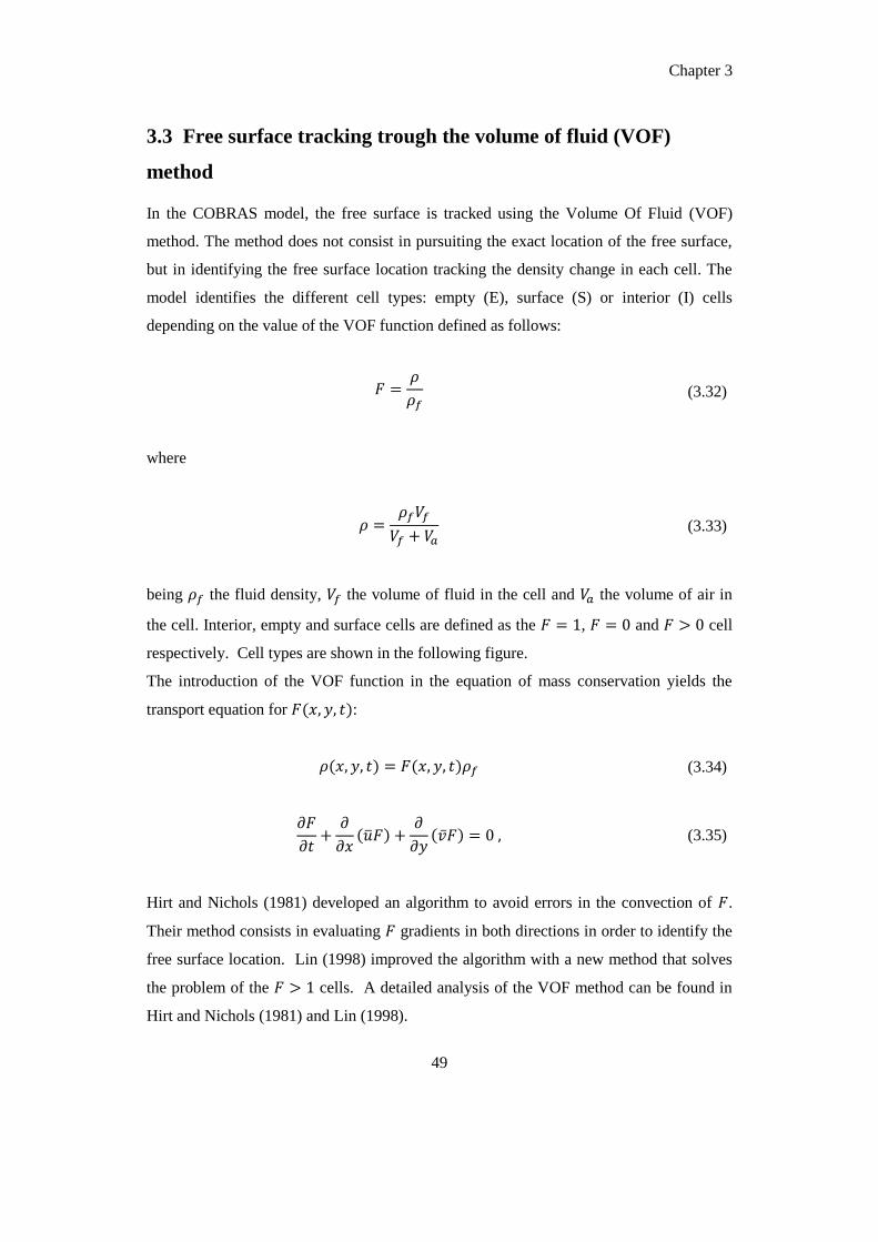
Chapter 3

49

3.3 Free surface tracking trough the volume of fluid (VOF)

method

In the COBRAS model, the free surface is tracked using the Volume Of Fluid (VOF)

method. The method does not consist in pursuiting the exact location of the free surface,

but in identifying the free surface location tracking the density change in each cell. The

model identifies the different cell types: empty (E), surface (S) or interior (I) cells

depending on the value of the VOF function defined as follows:

(3.32)

where

(3.33)

being the fluid density, the volume of fluid in the cell and the volume of air in

the cell. Interior, empty and surface cells are defined as the , and cell

respectively. Cell types are shown in the following figure.

The introduction of the VOF function in the equation of mass conservation yields the

transport equation for :

(3.34)

(3.35)

Hirt and Nichols (1981) developed an algorithm to avoid errors in the convection of .

Their method consists in evaluating gradients in both directions in order to identify the

free surface location. Lin (1998) improved the algorithm with a new method that solves

the problem of the cells. A detailed analysis of the VOF method can be found in

Hirt and Nichols (1981) and Lin (1998).

Chapter 3

50

3.4 Partial cell treatment

The IH-2VOF model allows the introduction in the computational domain of solid

boundaries of arbitrary shape, using a partial cell treatment. This method avoids the

potential spurious reflection at solid boundaries defined as sawtooth-shape surfaces fitting

the cell boundaries (Lemos, 1992). It consists in modelling the solid object as a special

case of fluid with an infinite density, introducing openness functions at the cell centre and

at the cell faces. At the cell centre, is defined as the ratio of space not occupied by the

solid object (thus open to the fluid) to the whole cell area. On the cell faces, ( ) is

defined as the length open to the fluid to the whole length of the right (top) boundary.

Therefore, similar to the VOF free surface tracking method, the model can identify

whether the cell corresponds to the solid object or obstacle (O), the fluid (air)-solid

boundary (FA-O) or the fluid (air) domain (FA). In order to solve the magnitudes defined

at the right face of the cells, the parameter identifies whether the cell face belongs to a

solid boundary or not. The only difference between the VOF function and the openness

functions is that the former is time-varying and the latter are not.

3.5 Governing equations for the flow in porous media (VARANS

equations)

To make the fluid/porous structure interaction modelling easier, a volume-averaging

process has been applied to the RANS and the and equations. The flow in porous

media is obtained in the IH-2VOF model through the resolution of the Volume-Averaged

Navier-Stokes (VARANS) equations. These equations are derived by integration of the

RANS equations over a control volume. The size of the averaging volume is chosen

much larger than the characteristic pore size but much smaller than the characteristic

length scale of the flow, i.e. the scale of the spatial variation of the physical variables in

the fluid domain.

The mathematical process of volume averaging of a certain quantity “a” is defined by the

following expression:

Chapter 3

51

⟨ ⟩

∫

(3.36)

where “⟨ ⟩” denotes the intrinsic volume averaging, is the total averaging volume,

is the volume in which is occupied by the fluid phase and ⟨ ⟩ is the averaged

magnitude. The intrinsic averaging operator defined by equation (3.36) can be related to

the Darcy’s volume averaging operator defined as follows:

⟨ ⟩

∫

(3.37)

through the simple relationship:

⟨ ⟩ ⟨ ⟩ (3.38)

where

(3.39)

is the porosity and is assumed for simplicity to be a constant in the present model. In

terms of velocity, ⟨ ⟩ would be the seepage velocity and ⟨ ⟩ the filtration velocity.

Hereafter, unless specified, volume averaging will be understood as intrinsic volume

averaging, as defined by expression (3.36).

To quantify the flow within the porous medium, the pore Reynolds number is defined as:

| |

(3.40)

where is the equivalent mean diameter of the porous material, is the fluid kinematic

viscosity and | | is a typical velocity scale around the pore.

Chapter 3

52

The VARANS equations are obtained by applying the intrinsic volume average to the

RANS equations. The ensemble averaged velocity of the RANS equations is assumed to

be:

⟨ ⟩ (3.41)

where ⟨ ⟩ is the ensemble-volume averaged velocity field and is the fluctuation with

respect to volume averaging, in other words the residual velocity field between ensemble-

volume averaging and ensemble averaging.

Applying this decomposition to the equations of continuity (3.2) and momentum

conservation (3.3), we obtain:

⟨ ⟩

(3.42)

⟨ ⟩

⟨ ⟩⟨ ⟩

⟨ ⟩

⟨

⟩

⟨ ⟩

⟨

⟩

∫ [

]

(3.43)

is the total fluid-solid interface and the jth component of the unit vector pointing

normally outward from the fluid to solid phase. The last term in equation (3.43) accounts

for the jump at the interface and represents the interfacial momentum transfer between the

fluid phase and the solid skeleton. This term is crucial in the modelling of the flow in

porous media. The previous term in the equation (3.44) is the residual stress due to

volume averaging: it results from the volume averaging of the convective term as:

⟨ ⟩ ⟨ ⟩⟨ ⟩ ⟨

⟩ (3.44)

analogously to the stress term in the Reynolds decomposition of the product . These

last two terms are unclosed and need to be modelled. Inside the porous media, these

Chapter 3

53

terms are modelled collectively using the Forchheimer’s relationship with the inclusion of

unsteady effects (Liu et al., 1999a):

⟨

⟩

∫ [

]

[

⟨ ⟩

√⟨ ⟩

⟨ ⟩ ⟨ ⟩

⟨ ⟩

]

(3.45)

where is the added mass coefficient and and two empirical coefficients associated

with the linear and nonlinear drag force respectively. The third term of the right-hand

side of equation (3.45) accounts for the inertial effects.

The precise descriptions of the , and coefficients are still not fully understood.

They depend a priori on the pore Reynolds number and flow directions. In their recent

study of wave motions and turbulent flows in front of a composite breakwater using the

COBRAS model, Hsu et al. (2002) propose the following values for these coefficients,

based on previous works by van Gent (1994), Liu et al. (1999a) or Nield and Bejan

(1999):

(3.46)

Finally, given the former closure expression for the residual stress term due to volume

averaging and the momentum transfer at the interface of equation (3.38), the complete

VARANS equations (3.38) and (3.39) can be rewritten as:

⟨ ⟩

(3.47)

⟨ ⟩

⟨ ⟩

⟨ ⟩

[

⟨ ⟩

⟨

⟩

⟨ ⟩

]

[

⟨ ⟩

√⟨ ⟩

⟨ ⟩ ⟨ ⟩]

(3.48)

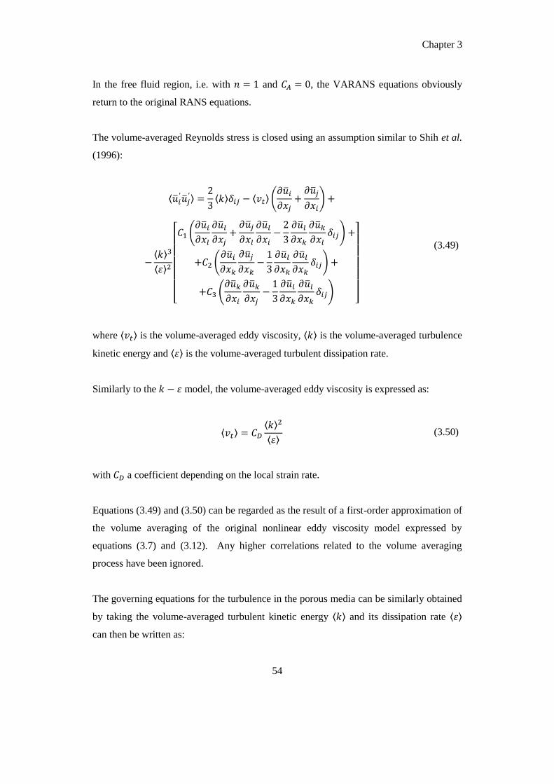
Chapter 3

54

In the free fluid region, i.e. with and , the VARANS equations obviously

return to the original RANS equations.

The volume-averaged Reynolds stress is closed using an assumption similar to Shih et al.

(1996):

⟨

⟩

⟨ ⟩ ⟨ ⟩ (

)

⟨ ⟩

⟨ ⟩

[ (

)

(

)

(

)

]

(3.49)

where ⟨ ⟩ is the volume-averaged eddy viscosity, ⟨ ⟩ is the volume-averaged turbulence

kinetic energy and ⟨ ⟩ is the volume-averaged turbulent dissipation rate.

Similarly to the model, the volume-averaged eddy viscosity is expressed as:

⟨ ⟩

⟨ ⟩

⟨ ⟩ (3.50)

with a coefficient depending on the local strain rate.

Equations (3.49) and (3.50) can be regarded as the result of a first-order approximation of

the volume averaging of the original nonlinear eddy viscosity model expressed by

equations (3.7) and (3.12). Any higher correlations related to the volume averaging

process have been ignored.

The governing equations for the turbulence in the porous media can be similarly obtained

by taking the volume-averaged turbulent kinetic energy ⟨ ⟩ and its dissipation rate ⟨ ⟩

can then be written as:

Chapter 3

55

⟨ ⟩

⟨ ⟩⟨ ⟩

⟨

⟩ ⟨ ⟩

[(

) ⟨ ⟩

] ⟨ ⟩

⟨

⟩

∫ (

)

⟨

⟩

(3.51)

⟨ ⟩

⟨ ⟩⟨ ⟩

⟨ ⟩

⟨ ⟩⟨

⟩ ⟨ ⟩

[(

) ⟨ ⟩

]

⟨ ⟩

⟨ ⟩

⟨ ⟩

⟨ ⟩⟨

⟩

∫ (

)

⟨

⟩

(3.52)

in which the following decompositions related to volume averaging have been assumed:

⟨ ⟩ (3.53)

⟨ ⟩ (3.54)

⟨

⟩

(3.55)

In both (3.51) and (3.52) equations, the fourth term on the right-hand side represents an

additional source term due to volume averaging. These terms describe the effects of

turbulence at a scale smaller than the volume-averaging scale, for instance the turbulence

generation in the wake region around the solid skeleton in high pore Reynolds number

conditions.

The fifth term represents the interfacial exchange of turbulence and is viewed as an

additional source or sink of turbulence due to the presence of solid materials. These two

terms are modelled collectively according to Nakayama and Kuwahara (1999),

substituted by in the ⟨ ⟩ transport equations and by the term:

(3.56)

in the ⟨ ⟩ transport equation.

Chapter 3

56

The last term on both ⟨ ⟩ and ⟨ ⟩ equations is the additional diffusion term due to the

volume averaging and can be combined with the existing diffusion terms in the ⟨ ⟩ and

⟨ ⟩ equations. The overall effect can be modelled by adjusting the values of and .

However, due to a lack of experimental information, the values of and are kept

unchanged in the IH-2VOF model. Therefore, the equations (3.51) and (3.52) can be

rewritten as:

⟨ ⟩

⟨ ⟩⟨ ⟩

⟨

⟩ ⟨ ⟩

[(

) ⟨ ⟩

] ⟨ ⟩ (3.57)

⟨ ⟩

⟨ ⟩⟨ ⟩

⟨ ⟩

⟨ ⟩⟨

⟩ ⟨ ⟩

[(

) ⟨ ⟩

]

⟨ ⟩

⟨ ⟩

(3.58)

The values of the closure coefficients, due to a lack of information here again, are kept

the same as those proposed by the standard model equations and the nonlinear eddy

viscosity model.

Expressions for the small-scale turbulence terms and have been proposed by

Nakayama and Kuwahara (1999), resulting from numerical simulations of flow passing

an array of square rods for pore Reynolds numbers between 105 and 10

7. The work by

Nakayama and Kuwahara (1999) for this range of values led to the following closure

forms:

⟨ ⟩ ⟨ ⟩

(3.59)

⟨ ⟩ ⟨ ⟩

(3.60)

To date, no work on the effect of the small-scale turbulence and expressions of and

for small values of the pore Reynolds number is available in the literature. However, it

can be verified that the small-scale turbulence represented by equations (3.59) and (3.60)

Chapter 3

57

has a negligible effect when the pore Reynolds number becomes small. Equations (3.59)

and (3.60) are thus expected to be still applicable in low pore Reynolds number

conditions.

3.6 Schematics of computational domain

The computational domain in the IH-2VOF model is discretised in rectangular cells as

sketched in Figure 3.1. The computing mesh can be divided into sub-mesh regions,

which allows a variable cells spacing: a finer grid can be defined for the representation of

specific study zones.

The different quantities in each of the cells are defined as follows: all scalar quantities,

i.e. pressure ( ), turbulent kinetic energy ( ), dissipation rate ( ), VOF function ( ) and

the hereafter specified openness function ( ) are defined in the centre of the cells. The

vector and vector-related quantities, i.e. the components of the mean velocity and the

additional openness functions ( and ), are defined on the cell faces as shown in

Figure 3.2. The x-component of the mean velocity is defined at the left face, the y-

component of the mean velocity is defined at the top face.

The IH-2VOF model allows the introduction in the computational domain of solid

boundaries of arbitrary shape, using a partial cell treatment. This method avoids the

potential spurious reflection at solid boundaries defined as sawtooth-shape surface4s

fitting the cell boundaries (Lemos, 1992). It consists in modelling the solid object as a

special case of fluid with an infinite density, introducing openness functions at the cell

centre and at the cell faces. At the cell centre,

Figure 3.1 and Figure 3.2 illustrate the definition of the different cell types based on the

information of the VOF function and openness functions.

Chapter 3

58

Figure 3.1. Schematics of computational domain with the different cell types on the information of the VOF

function and definition of the computed magnitudes (Lin, 1998).

Figure 3.2. Schematics of solid boundaries definition through the partial cell treatment (Lin, 1998).

Chapter 3

59

3.7 Numerical resolution

The finite difference method is used to solve the governing equations. A grid of points at

fixed locations is introduced in the spatial domain and the dependent variables are

initially defined and subsequently computed at these points. Approximate expressions for

derivatives appearing in the governing equations are found. These approximations are

formed using differences of dependent variables over finite space and time intervals. The

time step used in advancement of the evolution equations is the time scale of the

averaging of original Navier-Stokes equations. Then a system of algebraic equations that

approximates the governing partial differential equations is constructed.

The RANS equations are solved using the finite differences two-step projection method.

1. The first step is to introduce an intermediate velocity iu~ that does not satisfy the

continuity equation

(3.61)

where the superscripts denote the time level. This is the forward time difference

equation of the momentum equation in the RANS equation without the pressure

gradient term.

2. The second step is to project the intermediate velocity into a divergence free

plane to obtain the final velocity

(3.62)

(3.63)

Chapter 3

60

Taking the sum of the first and second step equations, the RANS momentum

equations are satisfied with the pressure gradient being evaluated at the (n+1)-th

time level

(3.64)

Taking the divergence of second step equation and applying continuity equation

yields we have

(

)

(3.65)

which is called the Poisson Pressure Equation (PPE).

In the two-step projection method, the spatial derivations of the velocity components and

the pressure field need to be expressed in finite-difference forms. The convection terms

are discretised by the combination of the central difference method and upwind method.

The combination of both is aimed at preventing their respective drawbacks of significant

numerical damping and numerical instability. A weighting factor is introduced in the

spatial derivative discretisation expressions in order to adjust the influence of each one of

the two schemes in the computation and to obtain stable and accurate solutions. Only the

central difference method is employed to discretise the pressure gradient terms and stress

terms.

Similarly to the Reynolds equations, the equations are solved by discretising the

convective terms with the combined central difference and upwind methods.

The detailed implementation of the numerical model can be found in Liu and Lin (1997)

and Lin (1998).

Chapter 3

61

3.8 Resolution procedure

The basic resolution procedure of IH-2VOF to update the field variables at a given time

step is summarised as follows:

compute intermediate velocities using equation (3.51);

apply the boundary conditions at the free surface and definition of the source

function;

compute the pressure value from equation (3.55);

obtain the final values of velocities from equation (3.54);

apply newly the boundary conditions at the free surface;

update VOF function values;

apply the boundary conditions at the newly fluid cells (empty at the previous time

step) consecutively to VOF function updating.

CHAPTER 4

REPRESENTATION OF THE WAVE

OVERTOPPING PROCESS.

The goal of this chapter is to analyze the overtopping process, in particular the layer

thicknesses and the velocities of the flow over the crest of a emerged/submerged

structures, in order to extend the existing theoretical approaches and provide criteria for

the design of structures close to mean sea level or overwashed. This analysis was carried

out on a numerical database derived by running the Rans-Vof code (IH-2VOF) in

presence of impermeable structures characterized by different slopes and freeboard.

In particular, we chose to investigate seadikes in order to compere our work with the

extensive work that it is possible find in literature (Schüttrumpf, 2001; Van Gent,2002;

Schüttrumpf and Van Gent, 2003; Schuttrumpf and Oumeraci, 2005; Eurotop, 2007).

However, the analysis can be extended to other types of coastal defences, for example,

breakwaters that are more frequently present in Italian coasts.

Figure 4.1. Severe wave overtopping at the Samphire Hoe seawall, UK (CLASH project, www.clash-eu.org,

2001).

http://www.clash-eu.org/

Chapter 4

63

4.1 Design criteria for coastal defences structures

Different types of coastal structures are built worldwide to protect low lying areas from

coastal flooding in coastal areas. Steep sea walls (slopes between 1:1.5 and 1:3) are used

in some coastal areas which are in general constructed of concrete, blocks or placed

stones. In Belgium, the Netherlands, Denmark, Germany and Poland, smooth seadikes

(slopes between 1:3 and 1:7) which are built of clay and sand are preferred. Thus, the

failure mechanisms of seadikes and seawalls differ significantly and different design

methods are used. At present, wave overtopping is the most important design criteria for

seawalls, while wave run-up still represents the most important design criteria for

seadikes.

The history of seadike design has recorded many heavy storm surges and dike breaches

up to the middle of the last century. The heavy storm surges in the Netherlands in 1953,

and in Germany in 1962, with many fatalities in both countries, have significantly

changed the design philosophy of seadikes. The design of seadikes was essentially based

on the highest water level ever observed plus a safety margin during previous centuries.

This procedure was replaced by a deterministic design philosophy as a consequence of

the storm surges in 1953 and 1962 and the crest level of seadikes are now determined

using a design water level with specific exceedance frequencies and the corresponding

wave run-up height. Nevertheless, a design water level with specific exceedance

frequencies and the corresponding wave run-up height are subject to large uncertainties,

so that wave overtopping cannot always be avoided. Therefore, wave overtopping has to

be considered for the design of seadikes and a deterministic design philosophy should be

replaced by a probabilistic design philosophy for seadikes in the future.

Probabilistic design requires an improved under-standing of all physical processes

responsible for dike failures. One important aspect is the determination of those wave

overtopping parameters which are relevant for infiltration, erosion and consequently dike

failures. The present design of seadikes does not consider the interaction of wave

overtopping flow and soil mechanic properties. The design water level is calculated from

measured water levels and extrapolated by fitted statistical distributions including an

exceedance frequency which is specified as a function of the local conditions and the

Chapter 4

64

vulnerability of the flood prone area. The corresponding wave run-up height is calculated

from the incoming wave parameters at the design water level. Important investigations

about the determination of the wave run-up height were carried out by Wassing (1957),

Hunt (1959), Battjes (1974), Owen (1980), Tautenhain (1981) and Van der Meer and

Janssen (1995). The wave run-up and wave overtopping formulas by Van der Meer and

Janssen (1995) have now been adopted in many national recommendations for the design

of seadikes.

As mentioned above, a wave run-up height and an average overtopping rate are

inappropriate parameters for the determination of infiltration and erosion. Therefore, all

processes relevant to the wave overtopping flow parameters have to be determined.

These processes must be understood to describe the overtopping flow which will provide

the hydraulic boundary conditions for erosion, infiltration and slip failure analysis.

Empirical equations describing wave overtopping processes in terms of incident wave

conditions, structure geometry, and crest freeboard have been developed based on small-

and large-scale physical model tests of common structure geometries. In particular, in

literature it is possible to find some theories that describe flow depths and velocities over

the dike crest for emerged conditions, whereas for zero freeboard and submerged

conditions a theoretical approach that allows to know the flow characteristics over the

dike crest is not available. Economic constraints and environmental and aesthetic impact

often impose more practical levee designs having lower crown elevations with the

associated risk that some wave/surge overtopping will occur during extreme events. In

addition, the increase of frequency and intensity of storms, combined with the

uncertainties related to extreme events and climate change, pose serious challenges in the

long term design of defences from coastal flooding. Therefore it is more likely that in the

next future many dikes will operate for longer times at lower crest freeboards, i.e. close to

mean sea level or even overwashed. For design purposes, accurate estimates of the

statistics of overtopping waves in terms of flow depths, duration and especially velocities

for a set of climate conditions are needed and have to be combined with consolidated

criteria for identifying tolerable overtopping threshold. At the moment, the information

Chapter 4

65

available for overwashed dikes can be derived from the (limited) set of tests performed by

Hughes et al. (2012).

As regards emerged structures, recently formulae have been derived for maximum flow

depth and velocities on the crest and inner slope. These formulae are based on the

difference fictive wave run-up and the crest freeboard. This is a good measure to

determine the flow depths and velocities on the dike. These formulae have been

calibrated by two independent physical model test programs in different wave flumes.

One of the studies has been carried out by Schüttrumpf in Germany (Schüttrumpf, 2001).

He performed large and small scale model tests and determined the empirical coefficients.

The other study has been carried out on small scale by Van Gent (Van Gent, 2002). He

calibrated the formulae and determined the empirical coefficients as well. When these

two studies are compared appears a large difference. In fact, the empirical coefficient of

the flow depth equation was determined to be a factor 2.2 higher by Schuttrumpf than by

Van Gent, whereas they agreed about the empirical coefficient of the velocity equation.

They collectively wrote a paper (Schuttrumpf and Van Gent, 2003) and found the test set-

up as primary cause for the discrepancy in the flow depth coefficient (see also

Schuttrumpf and Oumeraci, 2005). Bosman et al. (2008) used the raw data of

Schüttrumpf (2001) and van Gent (2002) and analyzed them using a new approach. He

shown that the outer slope is of great importance in the flow depths and velocities on the

crest. Whereas Schüttrumpf performed his tests on a dike model with an outer slope of

1:6, Van Gent used a dike model with outer slope of 1:4. Bosman verified that the

empirical coefficients are depending on the outer slope steepness. Therefore formulae for

maximum flow depth and velocity were adapted: the coefficients are written as a function

of the outer slope angle.

Moreover full-scale testing of dike landward slopes under a given sequence of

overtopping wave volumes through the Wave Overtopping Simulator (Van der Meer et

al., 2006, 2008, 2009) significantly extended our knowledge of landward-side dike

resiliency (Hoffmans et al., 2008; Van der Meer et al., 2010). However, the WOS

requires an accurate estimate of the wave overtopping volumes and related statistics to

Chapter 4

66

allow in cascade an accurate reproduction of flow depths and velocities on landward

slopes.

All formulae reported in this chapter are proposed by Eurotop manual (2007) which

summarizes all the existing theories.

4.2 Overtopping over a seadikes

Wave overtopping occurs if the crest level of the dike is lower than the highest wave run-

up level. In that case, the freeboard , defined as the vertical difference between the still

water level and the crest height, becomes important. Hence wave overtopping

depends on the freeboard and increases for decreasing freeboard height .

An exact mathematical description of the wave run-up and wave overtopping process for

coastal dikes is not possible due to the stochastic nature of wave breaking and wave run-

up and the various factors influencing the wave run-up and wave overtopping process.

Therefore, wave run-up and wave overtopping for coastal dikes are mainly determined by

empirical formulas derived from experimental investigation. The influence of roughness

elements, wave wall, berms, etc. is taken into account by introducing influence factors.

4.2.1 Wave overtopping discharge

In the case of emerged structures (positive freeboard) the Eurotop 2007 suggests the

following distinction (Figure 4.2).

Probabilistic design and prediction or comparison of measurements

( ). The following overtopping formulae for breaking and non-

breaking waves describes the average overtopping discharge:

√

√ (

)

(4.1)

with a maximum of:

Chapter 4

67

√

(

)

(4.2)

The reliability of Equations 4.1 and 4.2 are described by taking the coefficients

4.75 and 2.6 as normally distributed stochastic parameters with means of 4.75 and

2.6 and standard deviations and 0.35 respectively. For probabilistic

calculations Equations 4.1 and 4.2 should be taken together with these stochastic

coefficients. For predictions of measurements or comparison with measurements

also Equations 4.1 and 4.2 should be taken with, for instance, 5% upper and

lower exceedance curves.

Deterministic design or safety assessment ( ). For deterministic

calculation in design or safety assessment it is strongly recommended to increase

the average discharge by about one standard deviation. Thus, Equation 4.3

should be used for deterministic calculations in design and safety assessment:

√

√ (

)

(4.3)

with a maximum of:

√

(

)

(4.4)

In the case of very heavy breaking on a shallow foreshore the wave spectrum is

often transformed in a flat spectrum with no significant peak. In that case, long

waves are present and influencing the breaker parameter . Other wave

overtopping formulae are recommended for shallow and very shallow foreshores

to avoid a large underestimation of wave overtopping by using formulae 4.1, 4.2,

Chapter 4

68

4.3 and 4.4. Since those formulae are valid for breaker parameters a

linear interpolation is recommended for breaker parameters .

Deterministic design or safety assessment ( ). The following

formula is recommended including a safety margin for deterministic design and

safety assessment.

√

[

( )]

(4.5)

Probabilistic design and prediction or comparison of measurements

( ). The following formula was derived from measurements with a

mean of -0.92 and a standard deviation of 0.24:

√

[

( )]

(4.6)

Figure 4.2. Wave overtopping and overflow for positive, zero and negative freeboard (by Eurotop 2007).

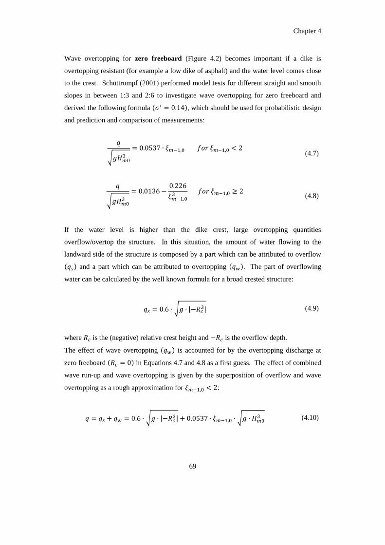
Chapter 4

69

Wave overtopping for zero freeboard (Figure 4.2) becomes important if a dike is

overtopping resistant (for example a low dike of asphalt) and the water level comes close

to the crest. Schüttrumpf (2001) performed model tests for different straight and smooth

slopes in between 1:3 and 2:6 to investigate wave overtopping for zero freeboard and

derived the following formula , which should be used for probabilistic design

and prediction and comparison of measurements:

√

(4.7)

√

(4.8)

If the water level is higher than the dike crest, large overtopping quantities

overflow/overtop the structure. In this situation, the amount of water flowing to the

landward side of the structure is composed by a part which can be attributed to overflow

and a part which can be attributed to overtopping . The part of overflowing

water can be calculated by the well known formula for a broad crested structure:

√ | | (4.9)

where is the (negative) relative crest height and is the overflow depth.

The effect of wave overtopping is accounted for by the overtopping discharge at

zero freeboard in Equations 4.7 and 4.8 as a first guess. The effect of combined

wave run-up and wave overtopping is given by the superposition of overflow and wave

overtopping as a rough approximation for :

√ | | √

(4.10)

Chapter 4

70

4.2.2 Overtopping flow velocities and overtopping flow depth

Average overtopping rates are not appropriate to describe the interaction between the

overtopping flow and the failure mechanisms (infiltration and erosion) of a clay dike.

Therefore, research was carried out recently in small and large scale model tests to

investigate the overtopping flow velocities and the related flow depth on the seaward

slope, the dike crest and the landward slope. Results are summarized in Schüttrumpf and

Van Gent (2003). Empirical and theoretical functions were derived and verified by

experimental data in small and large scale. These parameters are required as boundary

conditions for geotechnical investigations, such as required for the analysis of erosion,

infiltration and sliding.

The parameters of overtopping flow velocities and overtopping flow depth will be

described separately for the seaward slope, the dike crest and the landward slope. Here

only the considerations about the flow over the dike crest is reported.

The overtopping tongue arrives as a very turbulent flow at the dike crest. Maximum flow

depth and overtopping velocities were measured in this overtopping phase over the crest.

The overtopping flow separation occurs at the middle and at the dike surface at the front

edge of the crest. No flow separation occurs at the middle and at the rear edge of the

crest. In the second overtopping phase, the overtopping flow has crossed the crest. Less

air in the overtopping flow but the flow itself is still very turbulent with waves in flow

direction and normal to flow direction. In the third overtopping phase, a second peak

arrives at the crest resulting in nearly the same flow depth as the first peak. In the fourth

overtopping phase, the air has disappeared from the overtopping flow and both

overtopping velocity and flow depth are decreasing. Finally, the overtopping flow nearly

stops on the dike crest for small overtopping flow depths. Few air is in the overtopping

water. At the end of this phase, the overtopping water on the dike crest starts flowing

seaward.

The overtopping flow depth on the dike crest depends on the width of the crest and the

co-ordinate on the crest (Figure 4.4) and the flow depth decreases due to the fact that

Chapter 4

71

the overtopping water is deformed. Thus, the decrease of the overtopping flow depth

over the dike crest can be described by an exponential function:

(

) (4.11)

with the overtopping flow depth on the dike crest, the horizontal coordinate on the

dike crest with at the beginning of the dike crest, the dimensional coefficient

for TMA spectra and 1.11 for natural wave spectra , and

the width of the dike crest (for to 3 m in prototype scale).

Figure 4.3. Definition sketch for overtopping flow parameters on the dike crest (by Eurotop 2007).

A theoretical function for overtopping flow velocities on the dike crest has been

developed by using the simplifies Navier-Stokes equations and the following

assumptions: the dike crest is horizontal; velocities vertical to the dike slope can be

neglected; the pressure term is almost constant over the dike crest; viscous effects in flow

direction are small; bottom friction is constant over the dike crest.

The following formula was derived from the Navier-Stokes equations and verified by

small and large scale model tests (Figure 4.4):

(

) (4.12)

Chapter 4

72

with the overtopping flow velocity on the dike crest; the overtopping flow

velocity at the beginning of the dike crest ; the coordinate along the dike

crest; the friction coefficient; and the flow depth at . From the Equation (4.12) it

is obviously that the overtopping flow velocity decreases from the beginning to the end of

the dike crest and this decrease is more marked for increasing surface roughness (Figure

4.6). But for flow depth larger than about 0.1 m and dike crest widths around 2-3 m, the

flow depth and velocity hardly change over the crest.

Figure 4.4. Overtopping flow velocity data vs overtopping flow velocity formulae (by Eurotop 2007).

Figure 4.5. Left side: influence of overtopping flow depth on overtopping flow velocity; right side: influence

of bottom friction on overtopping flow velocity (by Eurotop 2007)

Chapter 4

73

4.3 The numerical database

The simulations were performed in 1:10 scale in a numerical flume 52.3 m long and 1.5

m deep under irregular waves with different significant wave heights and peak period

characterized by Jonswap spectrum (Table 4.1).

Table 4.1. Characteristics of simulated tests.

αoff = 1:4 ; αin = 1:3 αoff = 1:4 ; αin = 1:2 αoff = 1:6 ; αin = 1:3

Rc/Hs Tests Hs

[m]

Tp

[s]

wd

[m] Tests

Hs

[m]

Tp

[s]

wd

[m] Tests

Hs

[m]

Tp

[s]

wd

[m]

-1

T1A

0.10

1.74

0.80

T1E

0.10

1.74

0.80

T1I

0.10

1.74

0.80 T2A 2.18 T2E 2.18 T2I 2.18

T3A 1.58 T3E 1.58 T3I 1.58

T4A 2.25 T4E 2.25 T4I 2.25

T5A

0.20

3.29

0.90

T5E

0.20

3.29

0.90

T5I

0.20

3.29

0.90 T5A 3.10 T5E 3.10 T5I 3.10

T7A 4.36 T7E 4.36 T7I 4.36

T8A 4.43 T8E 4.43 T8I 4.43

0

T9B

0.10

1.74

0.70

T9F

0.10

1.74

0.70

T9J

0.10

1.74

0.70 T10B 2.18 T10F 2.18 T10J 2.18

T11B 1.58 T11F 1.58 T11J 1.58

T12B 2.25 T12F 2.25 T12J 2.25

T13B

0.20

3.29

0.70

T13F

0.20

3.29

0.70

T13J

0.20

3.29

0.70 T14B 3.10 T14F 3.10 T14J 3.10

T15B 4.36 T15F 4.36 T15J 4.36

T16B 4.43 T16F 4.43 T16J 4.43

0.5

T17C

0.10

1.74

0.65

T17G

0.10

1.74

0.65

T17K

0.10

1.74

0.65 T18C 2.18 T18G 2.18 T18K 2.18

T19C 1.58 T19G 1.58 T19K 1.58

T20C 2.25 T20G 2.25 T20K 2.25

T21C

0.20

3.29

0.60

T21G

0.20

3.29

0.60

T21K

0.20

3.29

0.60 T22C 3.10 T22G 3.10 T22K 3.10

T23C 4.36 T23G 4.36 T23K 4.36

T24C 4.43 T24G 4.43 T24K 4.43

-1.5

T25D

0.10

1.74

0.85

T25H

0.10

1.74

0.85

T25L

0.10

1.74

0.85 T26D 2.18 T26H 2.18 T26L 2.18

T27D 1.58 T27H 1.58 T27L 1.58

T28D 2.25 T28H 2.25 T28L 2.25

T29D

0.20

3.29

1.00

T29H

0.20

3.29

1.00

T29L

0.20

3.29

1.00 T30D 3.10 T30H 3.10 T30L 3.10

T31D 4.36 T31H 4.36 T31L 4.36

T32D 4.43 T32H 4.43 T32L 4.43

Chapter 4

74

For each wave attack the wave steepness remains constant and close to 2%. All

simulations were carried out without the implementation of the turbulent model. The

model settings adopted are shown in Table 4.2.


Boundary Condition Mesh resolution

Seaward Landward cell width [m] cell height [m]

Hs - Tp

(Jonswap spectrum) absorption 0.02

Off-shore Dike crest In-shore

0.02÷0.05 0.02 0.02÷0.04

The dimensions of the structure (crest width and height) are constant while crest

freeboard , seaward and landward slopes are variable (Figure 4.6).

By combining different geometries and wave attacks, a total of 96 tests were carried out.

Figure 4.6. Tested levee cross section (model-scale units).

4.4 Validation of the model

In order to verify the numerical simulations, selected numerical results were compared

against experimental data and consolidated theoretical formulae. In particular, it was

verified that the wave reflection coefficients calculated numerically for each test were

compatible with the experimental results obtained by Zanuttigh et al. (2006). Moreover,

also the overtopping discharges were compared with the theoretical formula by Van der

Meer (Eurotop, 2007).

Chapter 4

75

4.4.1 Wave reflection coefficient

The reflection coefficients obtained by the simulations were compared in Figure 4.7,

4.8 and 4.9 with the data for smooth straight slopes that are included in the reflection

database by Zanuttigh and Van der Meer (2006). It is worthy to remark that this database

includes structures in design conditions ( , , sop>1%).

In these graphs all the numerical tests for the structures with different seaward and

landward slopes are shown. The values of for emerged and zero freeboard cases fall

perfectly in the range of the experimental values. As expected, submerged conditions

give lower values of , falling under the range of the experimental data or at least in its

bottom part. Notwithstanding the numerical values of appear to be slightly greater

than the experimental values. However, the numerical trends show two key issues in

agreement with the physical process: the greater the submergence and/or the lower the

wave height, the lower the reflection.

Figure 4.7. obtained by the experimental database for smooth straight (Zanuttigh and Van der Meer,

2006) and the numerical simulation characterized by and .

Chapter 4

76





Chapter 4

77

4.4.2 Overtopping discharge

Tables 4.3, 4.4 and 4.5 report the discharge calculated numerically and theoretically for

emerged structures, structures with freeboard zero and submerged structures respectively.

For emerged cases the theoretical discharge is calculated by Equation (4.3), for cases with

freeboard zero the formulae used are Equations (4.7) and (4.8) and, finally, Equation (4.3)

is used for submerged cases.

Both for emerged cases and cases with freeboard zero, the theoretical discharge is well

represented and the relative error remains always under about 28%. The following

figures (4.10 and 4.11) report this good agreement showing the theoretical discharge vs

the numerical one.

Table 4.3. Emerged cases: theoretical total discharge qth, numerical total discharge qnum, relative error Err

(%).

Tests qth qnum Err(%) Tests qth qnum Err(%) Tests qth qnum Err(%)

T17C 0.005 0.005 8.81 T17G 0.005 0.004 21.99 T17K 0.002 0.003 26.56

T18C 0.007 0.009 24.21 T18G 0.007 0.008 15.44 T18K 0.003 0.003 10.62

T19C 0.004 0.005 25.89 T19G 0.004 0.005 28.31 T19K 0.002 0.002 25.89

T20C 0.007 0.008 5.43 T20G 0.007 0.009 27.92 T20K 0.003 0.004 23.81

T21C 0.014 0.015 6.01 T21G 0.014 0.017 16.61 T21K 0.006 0.008 20.60

T22C 0.013 0.015 17.89 T22G 0.013 0.016 20.19 T22K 0.006 0.007 17.60

T23C 0.020 0.022 11.22 T23G 0.020 0.022 8.74 T23K 0.010 0.010 3.75

T24C 0.020 0.024 17.66 T24G 0.020 0.022 4.97 T24K 0.010 0.010 4.59

Table 4.4. Cases with freeboard zero: theoretical total discharge qth, numerical total discharge qnum,

relative error Err (%).

Tests qth qnum Err(%) Tests qth qnum Err(%) Tests qth qnum Err(%)

T9B 0.009 0.008 12.19 T9F 0.009 0.010 15.53 T17J 0.006 0.005 8.15

T10B 0.010 0.010 1.88 T10F 0.010 0.011 4.88 T18J 0.007 0.007 7.87

T11B 0.008 0.010 17.33 T11F 0.008 0.010 17.33 T19J 0.005 0.006 13.01

T12B 0.010 0.011 3.08 T12F 0.010 0.012 18.78 T20J 0.007 0.008 14.86

T13B 0.025 0.021 16.69 T13F 0.025 0.030 16.47 T21J 0.017 0.016 6.43

T14B 0.025 0.027 8.50 T14F 0.025 0.022 9.45 T22J 0.016 0.017 0.96

T15B 0.029 0.034 16.76 T15F 0.029 0.031 5.90 T23J 0.020 0.023 18.12

T16B 0.030 0.030 1.06 T16F 0.030 0.033 10.83 T24J 0.020 0.022 11.67

Chapter 4

78

Figure 4.10. Total numerical discharge versus total theoretical discharge for emerged cases.

Figure 4.11. Total numerical discharge versus total theoretical discharge for cases with zero

freeboard.

As regards submerged cases, by calculating the relative error, we can observe that there is

a good agreement between the numerical and theoretical overflow discharge, whereas the

differences for the overtopping discharge are more marked. However, this contribute is

very small and so it not affects too much the total results.

Chapter 4

79

Table 4.5. Submerged cases: theoretical/numerical overtopping discharge qwth/qwnum, theoretical/numerical

overflow discharge qsth/qsnum, relative error E(%).

Tests qwth qwnum E(%) qsth qsnum E(%)

T1A 0.009 0.011 21.12 1.879 1.787 4.89

T2A 0.010 0.011 6.13 1.879 1.724 8.25

T3A 0.008 0.009 12.14 1.879 1.812 3.59

T4A 0.011 0.011 5.21 1.879 1.764 6.15

T5A 0.027 0.019 27.60 1.879 1.877 0.10

T6A 0.026 0.022 13.94 1.879 1.865 0.76

T7A 0.003 0.004 23.78 1.879 1.873 0.32

T8A 0.003 0.004 16.28 1.879 1.907 1.48

T25D 0.009 0.010 11.10 3.452 3.121 9.61

T26D 0.010 0.012 11.69 3.452 3.307 4.21

T27D 0.008 0.009 4.83 3.452 3.316 3.95

T28D 0.011 0.011 4.02 3.452 3.398 1.57

T29D 0.027 0.028 2.85 3.452 3.298 4.47

T30D 0.027 0.030 13.57 3.452 3.320 3.83

T31D 0.003 0.003 11.01 3.452 3.182 7.84

T32D 0.003 0.003 16.65 3.452 3.247 5.95

T1E 0.009 0.010 8.67 1.879 1.771 5.74

T2E 0.010 0.011 8.08 1.879 1.739 7.49

T3E 0.008 0.009 4.37 1.879 1.912 1.73

T4E 0.01 0.012 12.87 1.879 1.788 4.85

T5E 0.027 0.024 9.68 1.879 1.873 0.33

T6E 0.026 0.022 15.10 1.879 1.748 6.99

T7E 0.003 0.004 20.08 1.879 1.858 1.11

T8E 0.003 0.003 20.65 1.879 1.844 1.89

T25H 0.009 0.008 9.10 3.452 3.290 4.70

T26H 0.010 0.012 11.69 3.452 3.187 7.69

T27H 0.008 0.009 12.06 3.452 3.278 5.06

T28H 0.011 0.010 7.33 3.452 3.303 4.33

T29H 0.027 0.023 15.02 3.452 3.081 10.77

T30H 0.027 0.024 8.31 3.452 3.208 7.09

T31H 0.003 0.003 9.19 3.452 3.126 9.45

T32H 0.003 0.003 16.27 3.452 3.247 5.96

T1I 0.006 0.0058 1.52 1.8793 1.8965 0.9176

T2I 0.007 0.0085 24.14 1.8793 1.8995 1.0773

T3I 0.005 0.0049 10.80 1.8793 1.9052 1.3806

T4I 0.007 0.0082 17.65 1.8793 1.9041 1.3221

T5I 0.018 0.0184 3.01 1.8793 1.8053 3.9353

T6I 0.017 0.0205 18.67 1.8793 1.9058 1.4125

T7I 0.021 0.0239 14.69 1.8793 1.8784 0.0455

T8I 0.021 0.0231 10.01 1.8793 1.9090 1.5828

T25K 0.006 0.0060 1.00 3.4524 3.4225 0.8664

T26K 0.007 0.0075 8.32 3.4524 3.4017 1.4689

T27K 0.006 0.0058 4.83 3.4524 3.3927 1.7296

T28K 0.007 0.0057 19.15 3.4524 3.2586 5.6138

T29K 0.018 0.0205 12.15 3.4524 3.2333 6.3466

T30K 0.018 0.0206 16.59 3.4524 3.6168 4.7615

T31K 0.021 0.0211 1.20 3.4524 3.5116 1.7144

T32K 0.021 0.0276 29.24 3.4524 3.1296 9.3503

Chapter 4

80

4.5 Flow height evolution over the dike crest

In this paragraph the effects of the structure design parameters on the trend of depths of

the flow over the crest are investigated. The values of % (flow depth exceeded by 2%

of the waves) and % (wave period exceeded by 2% of the waves) at the dike off-shore

edge are summarized in Table 4.6 for all the tests. All the numerical results are compared

with the theory reported in the paragraph 4.2.

4.5.1 Influence of the dike submergence and geometry

Figure 4.12 shows the wave height trend over the crest structure for a test characterized

by , s, and . It appears that in case of

and 𝑆 , the evolution of the wave height is similar to the

literature results in case of emerged structures (Schuttrumpf, 2001; Van Gent, 2002;

Schuttrumpf and Van Gent, 2003; Schuttrumpf and Oumeraci, 2005; Bosman, 2008), i.e

the wave height tends to decrease along the crest. By increasing the submergence, the

decay of the wave height is less marked and it completely disappears when

.

In Figure 4.13, the evolution of the overtopping flow depth on the dike crest is reported

for the structures with different . In the same graph the results obtained for the same

wave attack and different submergences are shown. As expected, irrespectively of the

submergence, the influence of the appears to be negligible. This means that the flow

remains always subcritical over the crest under a sufficient hydraulic head.

The same comparison is reported in Figure 4.14 between structures characterized by

different . As in Figure 4.14, the results obtained for the same wave attack and

different submergences are reported. It is possible to observe that, only in case of

and the variation of affect the evolution on the dike crest

of the overtopping flow depth and a slight discrepancy among the results is present.

Hence for emerged structures the wave decay over the crest is less marked decreasing the

seaward steepness.

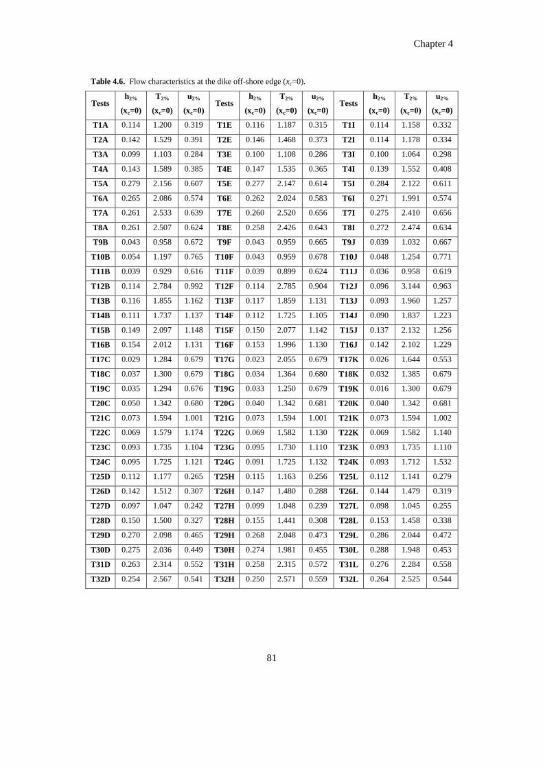
Chapter 4

81

Table 4.6. Flow characteristics at the dike off-shore edge (xc=0).

Tests h2%

(xc=0)

T2%

(xc=0)

u2%

(xc=0) Tests

h2%

(xc=0)

T2%

(xc=0)

u2%

(xc=0) Tests

h2%

(xc=0)

T2%

(xc=0)

u2%

(xc=0)

T1A 0.114 1.200 0.319 T1E 0.116 1.187 0.315 T1I 0.114 1.158 0.332

T2A 0.142 1.529 0.391 T2E 0.146 1.468 0.373 T2I 0.114 1.178 0.334

T3A 0.099 1.103 0.284 T3E 0.100 1.108 0.286 T3I 0.100 1.064 0.298

T4A 0.143 1.589 0.385 T4E 0.147 1.535 0.365 T4I 0.139 1.552 0.408

T5A 0.279 2.156 0.607 T5E 0.277 2.147 0.614 T5I 0.284 2.122 0.611

T6A 0.265 2.086 0.574 T6E 0.262 2.024 0.583 T6I 0.271 1.991 0.574

T7A 0.261 2.533 0.639 T7E 0.260 2.520 0.656 T7I 0.275 2.410 0.656

T8A 0.261 2.507 0.624 T8E 0.258 2.426 0.643 T8I 0.272 2.474 0.634

T9B 0.043 0.958 0.672 T9F 0.043 0.959 0.665 T9J 0.039 1.032 0.667

T10B 0.054 1.197 0.765 T10F 0.043 0.959 0.678 T10J 0.048 1.254 0.771

T11B 0.039 0.929 0.616 T11F 0.039 0.899 0.624 T11J 0.036 0.958 0.619

T12B 0.114 2.784 0.992 T12F 0.114 2.785 0.904 T12J 0.096 3.144 0.963

T13B 0.116 1.855 1.162 T13F 0.117 1.859 1.131 T13J 0.093 1.960 1.257

T14B 0.111 1.737 1.137 T14F 0.112 1.725 1.105 T14J 0.090 1.837 1.223

T15B 0.149 2.097 1.148 T15F 0.150 2.077 1.142 T15J 0.137 2.132 1.256

T16B 0.154 2.012 1.131 T16F 0.153 1.996 1.130 T16J 0.142 2.102 1.229

T17C 0.029 1.284 0.679 T17G 0.023 2.055 0.679 T17K 0.026 1.644 0.553

T18C 0.037 1.300 0.679 T18G 0.034 1.364 0.680 T18K 0.032 1.385 0.679

T19C 0.035 1.294 0.676 T19G 0.033 1.250 0.679 T19K 0.016 1.300 0.679

T20C 0.050 1.342 0.680 T20G 0.040 1.342 0.681 T20K 0.040 1.342 0.681

T21C 0.073 1.594 1.001 T21G 0.073 1.594 1.001 T21K 0.073 1.594 1.002

T22C 0.069 1.579 1.174 T22G 0.069 1.582 1.130 T22K 0.069 1.582 1.140

T23C 0.093 1.735 1.104 T23G 0.095 1.730 1.110 T23K 0.093 1.735 1.110

T24C 0.095 1.725 1.121 T24G 0.091 1.725 1.132 T24K 0.093 1.712 1.532

T25D 0.112 1.177 0.265 T25H 0.115 1.163 0.256 T25L 0.112 1.141 0.279

T26D 0.142 1.512 0.307 T26H 0.147 1.480 0.288 T26L 0.144 1.479 0.319

T27D 0.097 1.047 0.242 T27H 0.099 1.048 0.239 T27L 0.098 1.045 0.255

T28D 0.150 1.500 0.327 T28H 0.155 1.441 0.308 T28L 0.153 1.458 0.338

T29D 0.270 2.098 0.465 T29H 0.268 2.048 0.473 T29L 0.286 2.044 0.472

T30D 0.275 2.036 0.449 T30H 0.274 1.981 0.455 T30L 0.288 1.948 0.453

T31D 0.263 2.314 0.552 T31H 0.258 2.315 0.572 T31L 0.276 2.284 0.558

T32D 0.254 2.567 0.541 T32H 0.250 2.571 0.559 T32L 0.264 2.525 0.544

Chapter 4

82

Figure 4.12. Wave height trend on the dike crest for test T17C ( , red), T9B ( , blue),

T1A ( , green), and T25D ( , yellow).

Figure 4.13. Wave height trend on the dike crest for tests characterized by landward slope 1:3 (circles) and

1:2 (crosses) and different freeboard.

Chapter 4

83

Figure 4.14. Wave height trend on the dike crest for tests characterized by seaward slope 1:4 (circles) and


4.5.2 Comparison with the theory

The results obtained by the numerical analysis, i.e. wave height development on the dike

crest, are presented in the same way in which are presented in the theoretical approach

reported in Eurotop 2007 (Paragraph 4.2). The purpose of this analysis is to fit the

variation of the wave height over the dike crest by means of an appropriate curve and

identify the key parameters of such fitting.

The numerical results show that, as well as in semi-empirical formulation, the

overtopping wave height on the crest of the structure tends to exponentially decrease.

The wave height decay for each test was therefore fitted with an exponential curve and

the best fitting coefficient is reported in Table 4.7 for tests with 𝑆 , 𝑆

and 𝑆 . Even if each test is characterized by a specific decay coefficient, it

is possible to observe common trends of decay by grouping the tests with similar

submergence and wave attacks.

Chapter 4

84

The coefficients and the trend decay depend on the wave height whereas they do not

depend on the seaward/landward slope, hence six different average coefficients were

calculated for the three values of and the two of (see Table 4.8).

Table 4.7. Wave decay coefficients of the best fitting and relative standard deviation.

Tests ch σ' Tests ch σ' Tests ch σ'

Rc/Hs=0.5

Hs=0.1m

T17C 0.65 2.37 T17G 0.65 2.09 T17K 0.49 1.97

T18C 0.85 3.14 T18G 0.85 2.25 T18K 0.79 0.75

T19C 0.64 1.79 T19G 0.65 3.34 T19K 0.49 1.79

T20C 0.88 1.46 T20G 0.89 2.05 T20K 0.78 2.17

Rc/Hs=0.5

Hs=0.2m

T21C 0.36 2.97 T21G 0.37 2.87 T21K 0.32 3.51

T22C 0.36 0.60 T22G 0.39 3.37 T22K 0.32 4.21

T23C 0.59 2.31 T23G 0.58 2.48 T23K 0.45 2.56

T24C 0.61 2.37 T24G 0.61 2.62 T24K 0.48 2.21

Rc/Hs=0

Hs=0.1m

T9B 0.38 1.03 T9F 0.39 0.90 T9J 0.44 4.83

T10B 0.41 0.95 T10F 0.42 1.03 T10J 0.47 1.47

T11B 0.36 0.80 T11F 0.37 0.60 T11J 0.43 0.95

T12B 0.42 0.63 T12F 0.42 0.41 T12J 0.46 1.22

Rc/Hs=0

Hs=0.2m

T13B 0.25 1.76 T13F 0.24 1.82 T13J 0.30 0.67

T14B 0.24 1.57 T14F 0.24 1.83 T14J 0.29 2.49

T15B 0.38 0.99 T15F 0.29 0.88 T15J 0.39 0.42

T16B 0.28 1.49 T16F 0.29 1.62 T16J 0.33 3.98

Rc/Hs=-1

Hs=0.1m

T1A 0.12 0.80 T1E 0.11 0.67 T1I 0.10 0.61

T2A 0.17 0.32 T2E 0.17 0.36 T2I 0.13 0.42

T3A 0.11 0.20 T3E 0.12 0.21 T3I 0.09 0.39

T4A 0.17 0.21 T4E 0.27 0.28 T4I 0.15 0.23

Rc/Hs=-1

Hs=0.2m

T5A 0.07 0.28 T5E 0.08 0.35 T5I 0.06 0.28

T6A 0.06 0.23 T6E 0.06 0.27 T6I 0.05 1.07

T7A 0.12 0.47 T7E 0.12 0.44 T7I 0.10 0.19

T8A 0.12 0.37 T8E 0.12 0.39 T8I 0.10 5.21

In Figures 4.15 and 4.16 the tests with and m and

are shown respectively. Figure 4.17 and 4.18 show the numerical results for tests with

and with and respectively. Finally, Figure 4.19

and 4.20 show the results for tests with and with and

. Black curves are the fitting curves (obtained by the average coefficients of

Chapter 4

85

Table 4.8) that provides an overall fair approximation, with a decreasing of the quality

(for both wave height) in the second half of the crest.

By observing these graph, it immediately appears that the decay is much more marked as

the structure is emerged. For this reason this analysis has not been done for the cases

with because for those tests the decay is negligible.

Table 4.8. Average wave decay coefficients and relative standard deviation for each tests.

Average

coefficient Tests σ' Tests σ' Tests σ'

Rc/Hs=0.5

Hs=0.1m 0.72

T17C 3.79 T17G 3.42 T17K 8.62

T18C 5.24 T18G 4.77 T18K 2.44

T19C 3.50 T19G 4.21 T19K 9.13

T20C 5.74 T20G 5.87 T20K 3.17

Rc/Hs=0.5

Hs=0.2m 0.45

T21C 4.21 T21G 3.93 T21K 5.45

T22C 4.01 T22G 3.92 T22K 6.24

T23C 6.05 T23G 6.37 T23K 2.55

T24C 7.19 T24G 7.62 T24K 2.48

Rc/Hs=0

Hs=0.1m 0.38

T9B 1.04 T9F 0.95 T9J 2.72

T10B 1.82 T10F 2.13 T10J 3.99

T11B 1.17 T11F 0.82 T11J 2.53

T12B 1.72 T12F 1.53 T12J 3.93

Rc/Hs=0

Hs=0.2m 0.28

T13B 2.47 T13F 2.78 T13J 1.05

T14B 2.52 T14F 2.33 T14J 2.17

T15B 0.94 T15F 0.92 T15J 2.81

T16B 1.47 T16F 1.58 T16J 1.36

Rc/Hs=-1

Hs=0.1m 0.13

T1A 0.66 T1E 1.34 T1I 1.55

T2A 1.89 T2E 2.03 T2I 0.43

T3A 1.17 T3E 1.09 T3I 2.57

T4A 1.88 T4E 2.02 T4I 0.90

Rc/Hs=-1

Hs=0.2m 0.09

T5A 0.95 T5E 1.00 T5I 1.69

T6A 1.67 T6E 1.54 T6I 1.31

T7A 1.72 T7E 1.80 T7I 0.73

T8A 1.65 T8E 1.76 T8I 0.72

Chapter 4

86

Figure 4.15. Wave height decay on the dike crest with Hs=0.1m and . Squares: cases with

and ; triangles: cases with and ; diamonds: cases with

and .

Figure 4.16. Wave height decay on the dike crest with and . Squares: cases with


and .

Chapter 4

87



and .



and .

Chapter 4

88



and .



and .

Chapter 4

89

To understand the degree of approximation at the fitted formulation to the numerical data,

the standard deviation for each test was calculated (Table 4.5). The values of the standard

deviation remains always under about 9% suggesting that the approximation is very good

and in particular is more accurate for tests with = 0.1 m.

It is possible to observe that by keeping in constant the submergence, the wave height

decay tends to decrease, almost halved, when the significant wave height increases.

Similarly, the numerical results show that the wave height decay increases with

increasing the submergence when the significant wave height is constant.

4.5.3 Formula for the determination of the decay coefficient

The aim of this sub-paragraph is to understand if it is possible to predict the decay

coefficient that controls the decrease of the wave height over the dike crest. For example

it could exist a dependence on the wave attack, the characteristics structure and/or the

submergence.

An equation describing the trend of the dimensionless coefficient was derived. The

formula (Equation 4.14) shows the dependency of from:

- overtopping discharge;

- wave height;

- wave peak period;

- break parameter.

𝑆

√

(4.14)

where the total discharge (in case of submerged structures the sum for the contribute of

overflow and the overtop), is the wave height, the peak period, the water depth

and the Irribarren coefficient.

The three following Figures plot all data against Equation 4.14 and show that the trend is

different for different submergences. In fact, in Figure 4.21 the cases characterized by

are reported, whereas in Figure 4.22 and 4.23 the cases with

and are respectively represented. It is possible to approximate all points

Chapter 4

90

with a negative exponentially curve and, overall, there is a modest scatter with a

determination coefficient close to 0.95.



Chapter 4

91


4.6 Flow velocity evolution over the dike crest

In this paragraph the evolution of the flow velocity over the dike crest is described; in

particular the effects of the structure design parameters on the trend of velocities are

investigated. The values of % (flow velocity exceeded by 2% of the waves) at the dike

off-shore edge are summarized in Table 4.6 for all the tests. As for the wave height trend,

also the numerical results relative to the velocity are compared with the theory reported in

the paragraph 4.2.

4.6.1 Influence of the dike submergence and geometry

Figure 4.24 shows the evolution of the overtopping flow velocity by varying the

submergence. It can be observed that the velocity increases while the wave travels over

the crest, and specifically the growth rate decreases with increasing dike submergence.

Moreover, in the submerged cases, the decrease of flow depth (see Figure 4.12) and the

increase of velocity start from about the middle of the crest of the structure and however

are very modest.

Chapter 4

92

In Figure 4.25, the trends of the overtopping flow velocities on the dike crest are reported

for the structures with both landward slope 1:3 (represented as void circles) and 1:2

(represented as crosses). In the same graph the results obtained for different submergence

are shown. As regards the overtopping wave height, the influence of the landward slope

appears to be negligible. Only in case of (red color) a slight discrepancy among

the velocity results obtained for different seaward slopes is present.

Figure 4.26 compares the evolution of the overtopping flow velocities on the dike crest

for the 1:4 (represented as void circles) and 1:6 seaward slopes (represented as crosses).

It is possible to observe that, irrespectively of the submergence, the seaward slope does

not significantly affect the evolution on the dike crest of the overtopping flow velocity.

Figure 4.24. Flow velocity trend on the dike crest for test T17C ( , red), T9B ( , blue),

T1A ( , green) and T25D ( , yellow).

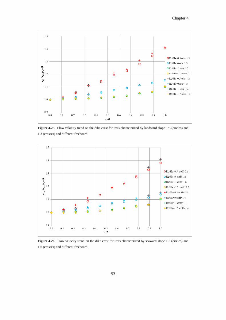
Chapter 4

93

Figure 4.25. Flow velocity trend on the dike crest for tests characterized by landward slope 1:3 (circles) and


Figure 4.26. Flow velocity trend on the dike crest for tests characterized by seaward slope 1:3 (circles) and


Chapter 4

94

4.6.2 Approximation of the velocity trend with a fitting function

The numerical tests show a slight increase of the velocity over the dike crest that can be

approximated with a second-order polynomial function. The best fitting coefficients for

each tests are reported in Tables 4.9. As for the wave heights, also the coefficients of the

velocity are found to be dependent on the wave height and not on the seaward/landward

slope. Hence, the average coefficients are reported in Table 4.10.

In Figure 4.27 and 4.28 tests with and the polynomial function obtained by

the average coefficients of Table 4.10 are respectively shown. The trend of the velocity

on the dike crest is very different for the tests with and . In the

cases with the velocity tends to increase from the beginning of the crest, in

the cases with there is a first phase of decrease and only after the middle of

the crest width the velocity starts to increase. The values of the standard deviation

reported (Table 4.10) remains under about 5% showing that the approximation is always

very good (irrespectively of the wave height).

Figure 4.29 and 4.30 compares the numerical results for tests with and the

polynomial function obtained by the average coefficients of Table 4.10. Tests with

and are respectively reported. Also in these cases, the trend of

the velocity on the dike crest is very different for the tests with different wave height. In

particular a continuous velocity growth is found for the tests with while for

the tests with the velocity tends first to decrease and then to increase starting

from the middle of the dike crest. By calculating the standard deviation for each test

(Table 4.10), it appears that the discrepancy from the curve remains always very low. In

particular, the approximation is better for tests with and the standard

deviation remains always under about 2.4%.

In the submerged case (Figures 4.31-4.32), for both wave heights, the trend of the

velocity on the dike crest tends to decrease and to increase starting from the middle of the

crest. The standard deviation for each tests (Table 4.10) remains under about 5%.

Chapter 4

95

Figure 4.27. Wave velocity evolution on the crest of the structure for tests with and

. Squares: cases with and ; triangles: cases with and ;

diamonds: cases with and .




Chapter 4

96

Figure 4.29. Wave velocity evolution on the crest of the structure for tests with and .

Squares: cases with and ; triangles: cases with and ; diamonds:

cases with and .

Figure 4.30. Wave velocity evolution on the crest of the structure for tests with and .

Squares: cases with and ; triangles: cases with and ; diamonds:

cases with and .

Chapter 4

97







Chapter 4

98

Table 4.9. Coefficients obtained with the best fitting curve for the wave velocity on the dike crest and

relative standard deviation.

Tests au bu σ' Tests au bu σ' Tests au bu σ'

Rc/Hs=0.5 Hs=0.1m

T17C 0.15 0.26 0.68 T17G 0.13 0.30 1.32 T17K 0.09 0.34 3.92

T18C 0.32 0.03 0.94 T18G 0.33 0.02 0.88 T18K 0.29 0.08 1.04

T19C 0.08 0.36 1.28 T19G 0.11 0.32 1.18 T19K 0.32 0.14 1.23

T20C 0.07 0.29 2.94 T20G 0.17 0.23 1.79 T20K 0.09 0.33 1.92

Rc/Hs=0.5

Hs=0.2m

T21C 0.43 -0.22 1.51 T21G 0.45 -0.24 1.73 T21K 0.44 -0.23 2.44

T22C 0.54 -0.41 1.98 T22G 0.54 -0.41 2.17 T22K 0.49 -0.23 1.81

T23C 0.55 -0.36 2.12 T23G 0.56 -0.37 2.34 T23K 0.58 -0.40 2.42

T24C 0.49 -0.36 1.93 T24G 0.49 -0.38 1.33 T24K 0.53 -0.43 1.51

Rc/Hs=0

Hs=0.1m

T9B 0.04 0.11 0.41 T9F 0.04 0.12 0.34 T9J 0.04 0.11 0.36

T10B 0.08 0.08 0.85 T10F 0.08 0.09 0.70 T10J 0.08 0.09 0.97

T11B 0.04 0.16 0.21 T11F 0.04 0.13 0.60 T11J 0.05 0.13 0.36

T12B 0.09 0.09 0.92 T12F 0.09 0.09 0.67 T12J 0.09 0.10 0.81

Rc/Hs=0

Hs=0.2m

T13B 0.26 -0.19 0.49 T13F 0.26 -0.19 0.57 T13J 0.28 -0.20 0.52

T14B 0.26 -0.19 0.39 T14F 0.25 -0.18 0.55 T14J 0.26 -0.18 0.37

T15B 0.25 -0.12 0.62 T15F 0.25 -0.12 0.54 T15J 0.25 -0.12 0.58

T16B 0.25 -0.12 0.45 T16F 0.24 -0.11 0.63 T16J 0.23 -0.10 0.64

Rc/Hs=-1

Hs=0.1m

T1A 0.13 -0.04 0.68 T1E 0.13 -0.03 0.73 T1I 0.13 -0.04 0.73

T2A 0.13 -0.07 0.76 T2E 0.14 -0.06 0.80 T2I 0.13 -0.06 0.60

T3A 0.13 -0.04 0.77 T3E 0.13 -0.03 0.73 T3I 0.13 -0.04 0.69

T4A 0.13 -0.05 0.56 T4E 0.12 -0.04 0.64 T4I 0.12 -0.04 0.48

Rc/Hs=-1

Hs=0.2m

T5A 0.08 -0.02 0.38 T5E 0.08 -0.02 0.47 T5I 0.08 -0.02 0.47

T6A 0.10 -0.02 0.23 T6E 0.11 -0.02 0.21 T6I 0.11 -0.02 0.23

T7A 0.10 -0.01 0.20 T7E 0.10 -0.02 0.20 T7I 0.10 -0.01 0.13

T8A 0.10 -0.01 0.14 T8E 0.10 -0.02 0.22 T8I 0.11 -0.02 5.13

Chapter 4

99

Table 4.10. Average coefficients for wave velocity evolution on the dike crest and relative standard

deviation for each tests.

Average coefficient

Tests σ' Tests σ' Tests σ' au bu

Rc/Hs=0.5 Hs=0.1m 0.18 0.22

T17C 0.82 T17G 1.80 T17K 1.27

T18C 5.31 T18G 5.18 T18K 4.19

T19C 2.71 T19G 2.20 T19K 2.48

T20C 3.62 T20G 1.93 T20K 1.44

Rc/Hs=0.5

Hs=0.2m 0.51 -0.35

T21C 3.27 T21G 2.70 T21K 2.53

T22C 3.94 T22G 4.20 T22K 2.34

T23C 1.84 T23G 2.19 T23K 2.73

T24C 3.30 T24G 3.83 T24K 5.02

Rc/Hs=0

Hs=0.1m 0.06 0.11

T9B 1.00 T9F 0.83 T9J 0.93

T10B 1.38 T10F 1.18 T10J 1.40

T11B 1.89 T11F 0.86 T11J 0.59

T12B 0.95 T12F 0.74 T12J 0.78

Rc/Hs=0

Hs=0.2m 0.25 -0.15

T13B 2.01 T13F 1.86 T13J 1.94

T14B 1.61 T14F 1.32 T14J 1.33

T15B 1.93 T15F 1.92 T15J 1.97

T16B 2.08 T16F 2.19 T16J 2.41

Rc/Hs=-1

Hs=0.1m 0.13 -0.05

T1A 1.23 T1E 1.39 T1I 1.33

T2A 0.89 T2E 0.78 T2I 0.79

T3A 1.33 T3E 1.23 T3I 1.25

T4A 0.57 T4E 0.82 T4I 0.71

Rc/Hs=-1

Hs=0.2m 0.09 -0.02

T5A 4.96 T5E 4.92 T5I 4.93

T6A 4.12 T6E 4.06 T6I 4.02

T7A 4.10 T7E 4.07 T7I 4.09

T8A 4.11 T8E 4.00 T8I 3.99

Chapter 4

100

4.7 Statistical characterization of extreme overtopping wave

volumes

In the design of coastal defences and in the estimate of their vulnerability a key aspect is

the realistic prediction of the characteristics of the overtopping waves. In fact

hydrodynamic forces on landward-side slopes largely depend on the distribution of

instantaneous overtopping wave volumes, flow thicknesses and flow velocities (Van der

Meer et al., 2010; Hughes et al., 2012). Overtopping wave volumes have been

successfully approximated by a Weibull distribution, whose shape factor appears to be

larger for very large overtopping and certainly for wave overtopping combined with

overflow (Hughes and Nadal, 2009; Victor, et al., 2012). The larger shape factor results

in lower maximum overtopping wave volumes.

The percent exceedance distribution of overtopping wave volumes is given by (Hughes et

al., 2012):

% [ (

)

] (4.15)

where % is the percentage of wave volumes that will exceed the specified volume ( ).

The two parameters of the Weibull distribution are the non-dimensional shape factor, ,

that helps define the extreme tail of the distribution and the dimensional scale factor, ,

that normalizes the distribution.

Hughes et al. 2012 valid the relationship of the Weibull shape factor for smooth and

impermeable structures like dikes and levees. The relationship is given as versus

to describe the distribution of overtopping wave volumes.

Zanuttigh et al. 2013 presents the analysis of the Weibull -value for conventional rubble

mound breakwaters as well as for low crested structures with the crest at or just above the

water level. It is concluded that rubble mound structures show more scatter in the -

value than smooth impermeable structures and the combined data make even more sense

Chapter 4

101

if the -value is related to relative discharge instead of relative freeboard because the

effects of slope angle and wave steepness are implicitly included.

In this analysis we compared our results with the new trend for the shape factor found

in Zanuttigh et al. 2013:

(

)

(4.16)

and in the following Figures data for smooth structure, different submergence and

seaward/landward steepness obtained by Hughes and Victor are reported.

Figure 4.33. Comparison numerical results ( ) with smooth structures against formula 4.16.

Chapter 4

102

Figure 4.34. Comparison numerical results ( , orange; , green; , pink;

, blue) with smooth structures against formula 4.16.

CHAPTER 5

TWO-PHASE APPROACH FOR SEDIMENT

TRANSPORT MODELLING.

The present chapter is devoted to the description of the modifications and improvements

that have been made in the IH-2VOF code in order to implement the sediment transport.

Most of these modifications have been carried out based on Hsu et al. 2004.

5.1 Governing equations for fluid and particle phase: RANS

equations

Sediment transport involves a fluid phase and a particle phase. The fluid phase is water

with mass density and the particle phase is represented as a identical spheres of

diameter and mass density . Assuming that the mixture can be treated as a

continuum, the ensemble averaged two-phase equations of mass and momentum can be

derived readily. In this averaging process, the definition of sediment concentration is

introduced. Because of the presence of the particle concentration, the two continuum

phases are, essentially, compressible. For this reason, we implement Favre averaging

(Favre 1965). For more details see Hsu et al. 2004.

The fluid and sediment phase continuity equations are:

(5.1)

(5.2)

where:

Chapter 5

104

(5.3)

and

(5.4)

In these equations and represent, respectively, the x-components of the fluid and

particle velocity and and the y-component of the fluid and particle velocity.

The x- and y- components of the fluid-phase momentum equations for the uniform flow

can be expressed as:

( )

(5.5)

and

( )

(5.6)

where is the fluid pressure,

are the fluid phase stresses and is the

gravitational acceleration. The last two terms in equations (5.5) and (5.6) are the Favre

averaged drag forces, with the drag coefficient defined as:

(

)

(5.7)

In Eq. (5.7), is the particle Reynolds number and is the magnitude of the relative

velocity between the fluid and sediment phase:

Chapter 5

105

(5.8)

√ (5.9)

where is the fluid viscosity and is a coefficient

(5.10)

The concentration dependence in equation (5.7) is taken from the experimental results of

Richardson and Zaki (1954). The drag force contribution in (5.5) and (5.6) is composed

of two terms. The first is the averaged drag force due to the relative mean velocity

between the two phases. The second, called fluid turbulent suspension, is the correlation

between the concentration and the large-scale fluid velocity fluctuations. It is modelled

here as a gradient transport (see McTigue, 1981).

The corresponding sediment-phase momentum equations are:

( )

(5.11)

and

( )

(5.12)

where

are the stresses of the sediment phase, including the small-scale

particle (inter-granular) stresses and the Reynolds stresses of the Favre averaged particle

Chapter 5

106

velocities. Closures for fluid turbulence and sediment stresses are major issues of sheet

flow modelling and are detailed in the next paragraph.

5.2 Closure of fluid stresses

Closures for fluid turbulence stresses in two-phase flows are very similar to the case of

clear water, with the exception of the contribution of sediment - in terms of concentration

and correlation between fluid and sediment velocities - in the governing equations for the

turbulent kinetic energy and for the rate of turbulent energy dissipation.

The total stress of the fluid-phase in equation (5.5) and (5.6) can be written as:

(5.13)

(5.14)

(5.15)

(5.16)

where

are the averaged small-scale stresses consisting of the viscous

stress and the small-scale Reynolds stress of the turbulence generated in the fluid between

the sediment particles or induced by fluctuations of the particles. The large-scale fluid

Reynolds stresses, defined as the correlations between the concentration and fluid

velocity fluctuations and ,

(5.17)

(5.18)

Chapter 5

107

(5.19)

(5.20)

result from the Favre averaging process. They represent the transfer of momentum that

occurs on the scale at which the concentration fluctuates.

The turbulent eddy viscosity hypothesis is used here to model the large-scale fluid

Reynolds stresses:

( )

(5.21)

( )

(5.22)

and

( )

(5.23)

( )

(5.24)

where is the kinematic viscosity of the fluid and is the fluid-phase turbulent kinetic

energy, defined as

(5.25)

The second term on the right-hand side of equations (5.23) and (5.24) appears because the

divergence of the fluid-phase velocity is not zero. We assume that the fluid phase eddy

viscosity is given by:

Chapter 5

108

(5.26)

where is an empirical coefficient and

(5.27)

is the fluid-phase turbulent dissipation rate. Because and appear in the eddy

viscosity, we need to introduce balance equations for both.

Following Hsu et al. (2004), the fluid phase turbulent kinetic energy equation in the

uniform flow can be written as

[(

)

]

[(

)

]

( )

( )

(5.28)

The last term in eq. (5.28), which originally involves correlations between fluctuations of

fluid and sediment velocities, represents a dissipation mechanism for the turbulent

energy, where is a parameter that measures the degree of correlation between the fluid

and sediment velocity fluctuations. It is determined by the relative magnitudes of a

particle response time , the time between collisions , and the fluid turbulence time-

scale :

(

)

(5.29)

The particle response time is defined as

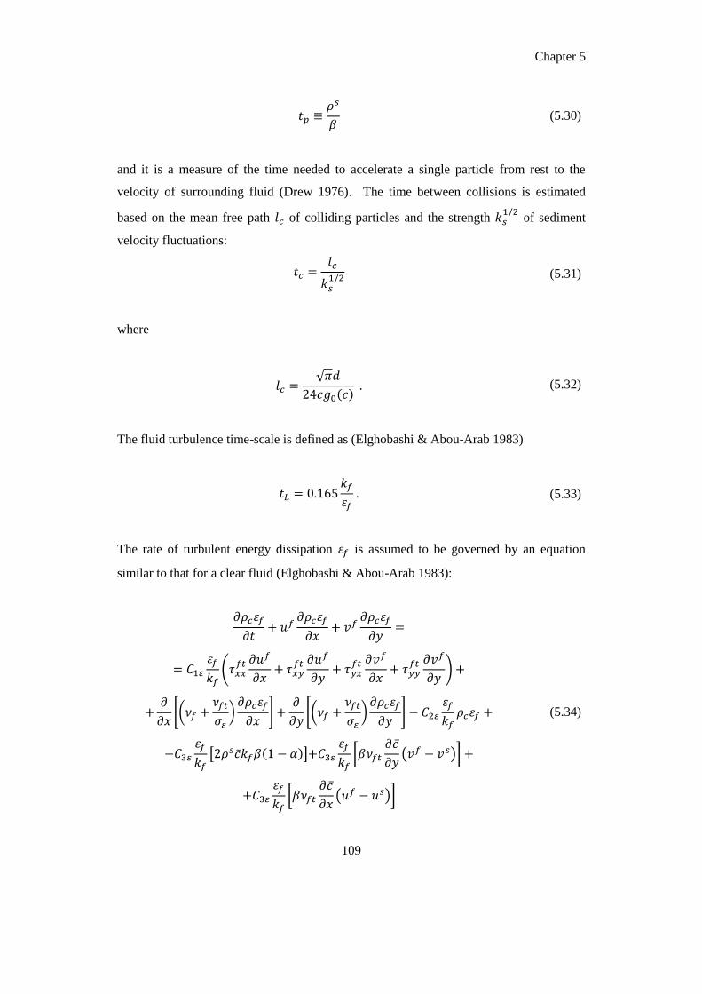
Chapter 5

109

(5.30)

and it is a measure of the time needed to accelerate a single particle from rest to the

velocity of surrounding fluid (Drew 1976). The time between collisions is estimated

based on the mean free path of colliding particles and the strength

of sediment

velocity fluctuations:

(5.31)

where

√

(5.32)

The fluid turbulence time-scale is defined as (Elghobashi & Abou-Arab 1983)

(5.33)

The rate of turbulent energy dissipation is assumed to be governed by an equation

similar to that for a clear fluid (Elghobashi & Abou-Arab 1983):

(

)

[(

)

]

[(

)

]

[ ]

[

( )]

[

( )]

(5.34)

Chapter 5

110

Due to the lack of information regarding the appropriate values of numerical coefficient

in the present model, we employ the same coefficients as those implemented in

the standard model for a clear fluid flow as already done by Hsu (see Hsu et al.

2004).

(5.35)

5.3 Closure of sediment stresses

In the sediment momentum equations, the two-scale averaging process results in a

sediment stress, which can be written as

(5.36)

(5.37)

(5.38)

(5.39)

where

are the mean particle shear and normal stresses due to small scale

interactions, while

are components of the large-scale sediment

Reynolds stress.

The small-scale stresses

are mainly due to granular interactions

resulting from particle collisions or interstitial fluid effects. Here, we adopt the kinetic

theory for collisional granular flow (Jenkins & Hanes 1998) for their closure.

Following this theory, the transport coefficients in the constitutive relations for

are obtained from the kinetic theory of dense gases (Chapman &

Cowling 1970). The particle normal and shear stresses due to collision are represented

as:

Chapter 5

111

(5.40)

(

) (5.41)

(5.42)

where , with the radial distribution function at contact for identical

spheres.

Torquato (1995) provides an accurate expression for this radial distribution function that

is good for concentrations between 0.49, at which a phase transition between random and

hexagonal packing is first possible, and the random close-packed concentration,

, at which the mean distance between the edges’ nearest neighbors is zero:

{

(5.43)

where .

The product in eq. (5.40) and (5.42) is the sediment viscosity due to collisions and

we have:

(

)

⁄

⁄

(5.44)

(

)

(5.45)

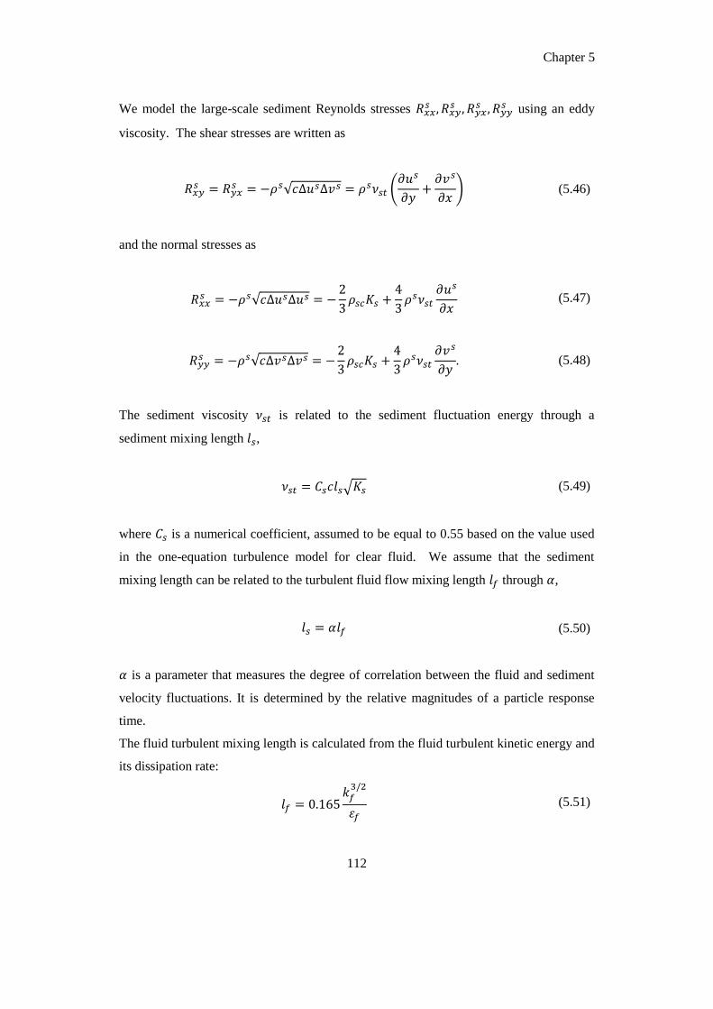
Chapter 5

112

We model the large-scale sediment Reynolds stresses

using an eddy

viscosity. The shear stresses are written as

√ (

) (5.46)

and the normal stresses as

√

(5.47)

√

(5.48)

The sediment viscosity is related to the sediment fluctuation energy through a

sediment mixing length ,

√ (5.49)

where is a numerical coefficient, assumed to be equal to 0.55 based on the value used

in the one-equation turbulence model for clear fluid. We assume that the sediment

mixing length can be related to the turbulent fluid flow mixing length through ,

(5.50)

is a parameter that measures the degree of correlation between the fluid and sediment

velocity fluctuations. It is determined by the relative magnitudes of a particle response

time.

The fluid turbulent mixing length is calculated from the fluid turbulent kinetic energy and

its dissipation rate:

(5.51)

Chapter 5

113

For massive particles with a long particle response time, , the fluid turbulent eddies

cannot induce any sediment velocity fluctuations, and . For fine particles with

small particle response time, , the fine particles follow the turbulent eddies, and

.

The kinetic theory of dense gases is based on the fundamental assumption of a significant

number of collisions. Therefore, when the sediment concentration becomes very dilute,

the validity of the collisional grain flow theory becomes questionable. Therefore, we

introduce a damping parameter for the small-scale sediment stress defined in terms of

the mean free path of the sediment particles and the fluid turbulent mixing length ,

(5.52)

When the mean free path of collision becomes much larger than the fluid turbulent

mixing length, the small-scale collisional transport is reduced through a diminishing .

The constitutive relations for particle collisions based on the kinetic theory of dense

molecular gases have been successfully implemented to study problems of rapid granular

flow at concentrations smaller than the random loose packing . The primary reason for

the close similarity between particle and molecular collisions is that they are of relatively

short duration, compared with the time between collisions. However, for granular

shearing flows at concentrations greater than , particles are in enduring contact.

Therefore, the analogy between the particles and molecules is no longer valid.

Here, we model the sediment transport above the stationary bed, where the concentration

is near random close packing. Therefore, modifications to the collisional grain flow

theory for the closure of particle stress are needed. The discrete particle simulations of

Zhang & Campbell (1992) indicate that between the random close-packed concentration

and the random loose-packed concentration , the granular material is in a transitional

state between solid-like and fluid-like behavior. Bocquet et al . (2001) carried out

experiments on the Couette flow of grains in this regime and observed that the viscosity

of the particle shear stress increased dramatically as the concentration approached .

They suggested that in the viscosity, the power in equation (33) should be changed

Chapter 5

114

from 1.00 to 1.75. That is, in our numerical implementation, is taken to be 1.00 when

and 1.75 when . Therefore, as far as the particle shear stress is concerned,

the region involving enduring contacts is modelled by taking the granular material to be

an extremely viscous fluid. As the concentration increases above , the collisional

contribution to the particle normal stress diminishes, because the shearing of the particle

phase that is the source of the collisional fluctuations becomes very small. However, in

this range of concentration, the contribution to particle normal stress due to enduring

contacts becomes important. Therefore, we further assume that the small-scale particle

normal stress and

is the sum of the collisional normal stress ( and

) and the

normal stress ( and

) due to enduring contact:

(5.53)

(5.54)

We model the collisional stress using equations (12) and (14), while for the normal stress

due to enduring contacts we adopt a Hertz contact relation. For a homogeneously packed,

dry granular material consisting of identical spheres in Hertzian contact, the normal stress

is (Jenkins et al . 1989)

(

)

(5.55)

where is the average compressive volume strain, is given in terms of the shear

modulus e and Poisson’s ratio of the material of the particles

√

(5.56)

and is the average number of contacts per particle or coordination number. We do not

solve Eq. (5.50) for , but assume that ⁄ can be related to the difference between the

local average concentration and that of random loose-packing by

Chapter 5

115

⁄ (5.57)

in which is a coefficient. Based on numerical experiments for plastic particles

implement ted by Sumer et al . (1996), gives a failure concentration of ca. 62%.

Therefore, this value is adopted.

Then

{

(5.58)

where the coordination number is taken to be a function of concentration.

[

(

)] (5.59)

Because appears both in the sediment viscosity and in the normal-shear stresses,

we need to introduce the transport equation for it (see Hsu 2002).

( )

(5.60)

with the flux of the fluctuation energy and the dissipation. The last term in the above

equation describes the interaction between the two phases. Therefore, there is an

additional source term, , due to the fluid turbulent kinetic energy. This term

models the influence of fluid turbulent eddies on the random motions of sediment

particles and permits turbulent eddies to enhance the sediment fluctuation energy.

Moreover, an additional dissipation mechanism, , also appears due to the drag of

the interstitial fluid.

The flux of sediment fluctuation energy is taken to be the sum of the small-scale

and the large-scale components:

Chapter 5

116

(5.61)

where:

(

) (5.62)

and

(

) (5.63)

being a numerical coefficient (1.0).

Based on the kinetic theory for collisional granular flow, M in eq. (5.57) is:

(

)

(5.64)

Finally, we take the dissipation rate in equation (5.60) to be the collisional dissipation

associated with the inelasticity of the particles. Based on the analysis of Jenkins &

Savage (1983), and considering as the coefficient of restitution (0.8), we can write:

[

(

)] (5.65)

Chapter 5

117

5.4 Model implementation

In order to solve the RANS equations both for fluid and sediment phase a method very

similar to the two-step projection method used in the original IH-2VOF has been

implemented. In the follow the method is described in detail.

1. An intermediate velocity both for fluid and sediment phase is introduced. These

velocities ( , , , ) does not, in general, satisfy the continuity equation

and derive from the momentum equation without the pressure gradient term.

For the x-direction is possible write

( )

( )

( )

( )

( )

( )

( )

[( )

( )

]

[

(

)

(

)

]

[ (( )

)

]

(5.66)

[( )

]

[

( )

]

[ (( )

)

]

(5.67)

and for the y-direction

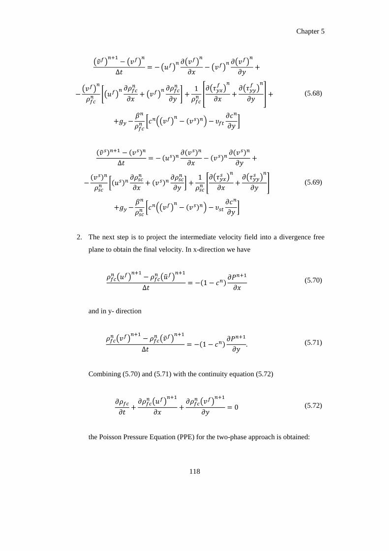
Chapter 5

118

( )

( )

( )

( )

( )

( )

( )

[( )

( )

]

[

(

)

(

)

]

[ (( )

)

]

(5.68)

[

]

[

( )

( )

]

[ (( )

)

]

(5.69)

2. The next step is to project the intermediate velocity field into a divergence free

plane to obtain the final velocity. In x-direction we have

( )

( )

(5.70)

and in y- direction

( )

( )

(5.71)

Combining (5.70) and (5.71) with the continuity equation (5.72)

( )

( )

(5.72)

the Poisson Pressure Equation (PPE) for the two-phase approach is obtained:

Chapter 5

119

(

)

(

)

[ ( )

( )

]

( )

( )

(5.73)

By solving (5.73) with the appropriate boundary conditions, the correct pressure

information at the n+1-th time step will be obtained.

3. Substituting the updated pressure information into (5.70) and (5.71), the new

velocity field for the fluid at the n+1-th time step, which satisfies the continuity

equation, is obtained. In the same way, by substituting the updated pressure

information into the following equations

(5.74)

(5.75)

also the new velocity field for the sediment at the n+1-th time step is obtained.

4. Finally, the new value of the concentration can be calculated on the base of the

continuity equation of the sediment phase at the n+1-th time step.

(5.76)

(5.77)

Chapter 5

120

5.5 Spatial discretization in finite different form

In the equations presented in the previous paragraph, spatial derivatives need to be

specified. The nonlinear advection terms are discretized by using a combination of the

upwind scheme and the central difference scheme to achieve an accurate numerical

solution. The central difference method is employed to discretize the pressure gradient

terms and stress gradient terms. Introducing the discretization of spatial derivatives into

the Poisson pressure equation yields a set of linear algebraic equations for the pressure

field that is solved using conjugate gradient method with the preconditioned of

incomplete Cholesky decomposition.

Stability of finite difference scheme is performed by Heuristic analysis. Implicit

discretization of the pressure term in the momentum equation leads to a linear system of

equations that needs considerable computational effort to be solved. However this kind

of discretization avoids any stability condition related to pressure term. On the other

hand, the explicit discretization of the advection and diffusion terms in the momentum

equation leading to a time step constraints such that

{

| |

| |} (5.78)

{

} (5.79)

are required.

The scheme implemented in the two-phase approach, as in the original IH-2VOF, is a

finite-different scheme. As shown in Figure 3.1, the scheme calculates the velocity

components of the fluid/sediment, and , on the vertical and horizontal cell

faces, respectively, whereas the pressure and other scalars such , , the volume of

fluid function and the sediment concentration , are defined at the cell center.

It is noted that in the finite difference form, some variables are needed at the place where

they are not originally defined, for example, the horizontal velocity at the top face of the

cell or the vertical velocity at the right face of the cell. In such circumstances, the linear

interpolation is used. In the follow the most commonly used interpolation variables are

Chapter 5

121

given and it is not specified the superscript or because the interpolation is the same

both for the fluid phase and the sediment phase.

(

) (5.80)

(

) (5.81)

(5.82)

(5.83)

(5.84)

(5.85)

(5.86)

( ) (5.87)

Chapter 5

122

5.5.1 Advection terms

Both for sediment and fluid equations, in equations (5.66), (5.67), (5.68) and (5.69) all

the advection terms will be evaluated at the n-th time step. The advection terms in the x-

momentum equation

are evaluated at the right face of the cell. The advection

terms in the y-momentum equation

are evaluated at the top face of the cell.

(

)

(

)

(5.88)

(

)

(

)

(5.89)

As in Lin and Liu (1998), also here to calculate the spatial derivatives of the velocity the

combination of the upwind scheme and the central difference scheme is used. The

upwind scheme is represented by

(

)

{

(

)

(

)

(5.90)

and the center difference scheme is represented by

(

)

(

)

(

)

(5.91)

In both (5.90) and (5.91)

Chapter 5

123

(

)

(5.92)

(

)

(5.93)

are defined. Since the upwind scheme usually introduces significant numerical damping

and the central difference scheme generates numerical instability, a combination of these

two schemes usually yields a more accurate numerical solution. Thus, the general

formula for the spatial derivative becomes

(

)

[ (

)] (

)

[ (

)] (

)

(

)

(5.94)

and similarly

(

)

[ (

)] (

)

[ (

)] (

)

(

) (

)

(5.95)

where

(

)

(5.96)

and

Chapter 5

124

(

)

(5.97)

For the advection terms in the y-direction we have to define the following derivatives:

(

)

[ (

)] (

)

[ (

)] (

)

(

)(

)

(5.98)

and

(

)

[ (

)] (

)

[ (

)] (

)

(

) ( )

(5.99)

where

(

)

(5.100)

(

)

(5.101)

(

)

(5.102)

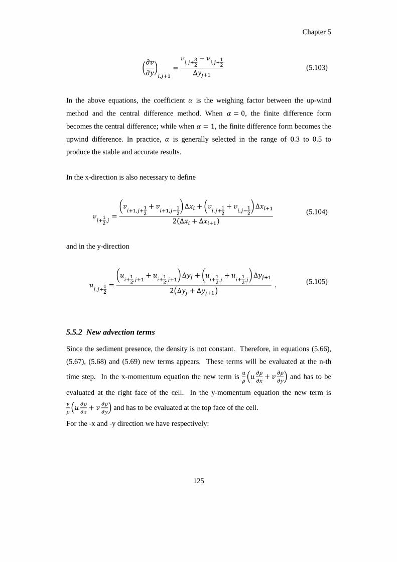
Chapter 5

125

(

)

(5.103)

In the above equations, the coefficient is the weighing factor between the up-wind

method and the central difference method. When , the finite difference form

becomes the central difference; while when , the finite difference form becomes the

upwind difference. In practice, is generally selected in the range of to to

produce the stable and accurate results.

In the x-direction is also necessary to define

(

) (

)

(5.104)

and in the y-direction

(

) (

)

( ) (5.105)

5.5.2 New advection terms

Since the sediment presence, the density is not constant. Therefore, in equations (5.66),

(5.67), (5.68) and (5.69) new terms appears. These terms will be evaluated at the n-th

time step. In the x-momentum equation the new term is

(

) and has to be

evaluated at the right face of the cell. In the y-momentum equation the new term is

(

) and has to be evaluated at the top face of the cell.

For the -x and -y direction we have respectively:

Chapter 5

126

[

(

)

(

)

] (5.106)

[

(

)

(

)

] (5.107)

where

(5.108)

(5.109)

(

)

(5.110)

(

)

(

)

( )( )(

)

(

)

(5.111)

(

)

(

)

(

)

(

)

(5.112)

Chapter 5

127

(

)

(5.113)

5.5.3 Tangential terms

5.3.3.1 Fluid phase

The gradient of the total stress for the fluid in Equation (5.66) is multiplied to

. This

term has to be defined in the first equation at the right face of the cell and in the second at

the top face (see equations 5.108 and 5.109 respectively).

The gradient of the total stresses in (5.66) can be written as

(5.114)

for the x-momentum equation and

(5.115)

for the y-momentum equation. Once again the stress gradient in the x-direction is

calculated at the right face of the computational cell, while in the y-direction it is

computed at the top face of the cell. Thus, the first term of 5.114 can be written in the

following finite difference from

(

)

(

)

(

)

(5.116)

The second term in 5.114 can be written as

Chapter 5

128

(

)

(

)

(

)

(5.117)

The total stresses (normal and shear) above are the summation of molecular stresses and

Reynolds stresses. The former are the products of the molecular viscosity and the strain

rates of the mean flow, and the latter can be obtained by the nonlinear algebraic Reynolds

stress model (5.118). Both of them involve the evaluation of the strain rates of the mean

flow. The normal stress in the x-direction is evaluated at the center of the cell which

involves the calculation of normal strain rate of the mean flow

(

)

( )

( )

(5.118)

The shear stress is evaluated at the vertices of the cell which involves the calculations of

both

and

. The finite difference form of these derivatives can be referred to (5.96)

and (5.97). the similar finite-difference formulas can be obtained for stress gradient terms

in the y-momentum equation (5.117). The shear strain rate of the mean flow can be again

referred to (5.96) and (5.97) and the normal strain rate at the cell in the y-direction is

expressed as

(

)

( )

( )

(5.119)

5.3.3.2 Sediment phase

Also the gradient of the total stress of the sediment phase is multiplied in Equation (5.67)

to

(see equations 5.108 and 5.109 respectively).

The gradients of the total stresses can be written as

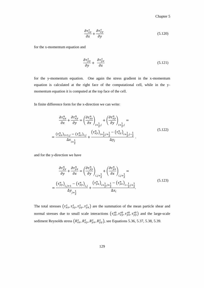
Chapter 5

129

(5.120)

for the x-momentum equation and

(5.121)

for the y-momentum equation. One again the stress gradient in the x-momentum

equation is calculated at the right face of the computational cell, while in the y-

momentum equation it is computed at the top face of the cell.

In finite difference form for the x-direction we can write:

(

)

(

)

( )

(

)

(5.122)

and for the y-direction we have

(

)

(

)

(

)

( )

( )

(

)

(5.123)

The total stresses (

) are the summation of the mean particle shear and

normal stresses due to small scale interactions (

) and the large-scale

sediment Reynolds stress (

), see Equations 5.36, 5.37, 5.38, 5.39.

Chapter 5

130

The mean particle shear and normal stresses due to small scale interactions for the x-

direction is

[

]

(

)

(5.124)

( )

[(

)

(

)

] (5.125)

and for the y-direction is:

( )

[

]

(

)

(5.126)

( )

[(

)

(

)

] (5.127)

In which (

)

is defined as in Equation (5.94), (

)

as in Equation (5.95),

(

)

as in Equation (5.98) and (

)

as in Equation (5.99). While (

)

and (

)

are defined as:

(

)

(5.128)

(

)

(5.129)

Chapter 5

131

In Equations (5.124) and (5.125),

and

depend on

:

(5.130)

and in Equations (5.126) and (5.127),

and

depend on

:

(5.131)

The Reynolds stresses for the x-direction are written as

(

)

(5.132)

( )

[(

)

(

)

] (5.133)

and for the y-direction as

( )

(

)

(5.134)

( )

[(

)

(

)

] (5.135)

Chapter 5

132

5.5.4 Drag force terms

As for the others terms, also the drag force terms are defined in the x-direction at the right

face of the numerical cell and in the y-direction at the top face.

( )

(

)

( )

(

)

(5.136)

( )

(

)

( )

(

)

(5.137)

where

(

)

(

)

(5.138)

(

)

(

)

(5.139)

(

)

(5.140)

(

)

(5.141)

Chapter 5

133

( )

( )

(

)

(5.142)

( )

( )

(

)

(5.143)

5.5.5 Pressure terms

Pressure is defined at the center of the computational cell, hence the Poisson Equation has

to be discretized calculating all terms at the center of the cell.

If we consider the right terms of Equation (5.73), we have:

[ (

)]

[ (

)]

{

[ (

)]}

{

[ (

)]}

{(

)(

)

(

)(

)

}

{(

)(

)

(

)(

)

}

(5.144)

where

(

)

(5.145)

Chapter 5

134

(

)

(5.146)

(

)

(5.147)

(

)

(5.148)

(5.149)

(5.150)

The left terms of the Equation (5.73) can be discretized as:

[ ( )

( )

]

( )

( )

( )

(

)

(

)

[(

( )

)

( ( )

)

]

( )

(

)

( )

(

)

(5.151)

where ( ( )

)

, ( ( )

)

, ( )

and ( )

are defined in Equations

(5.118), (5.119), (5.80) and (5.81), respectively. Whereas the derivatives of the density at

the centre of the computational cells are defined as following:

Chapter 5

135

(

)

(

)

( )

(

)

(5.152)

(

)

(

)

( ) ( )

( ) (

)

( )

( )( )

(5.153)

By this way, a set of linear algebraic equations for the pressure field that can be solved by

standard matrix solvers. Here the conjugate gradient method with the preconditioner of

incomplete Cholesky decomposition is used to solve the resulting sparse and symmetric

system of equations.

Solving the PPE equation the values of the pressure at the n+1 time step are determined

and the values of the sediment and fluid velocities and the concentration can be update.

CHAPTER 6

WAVE-INDUCED EROSION AND DEPOSITION

PATTERNS: VERIFICATION OF MODEL

RESULTS.

In this chapter a preliminary verification of the two-phase numerical model is presented.

Some simple cases were chosen in order to check all the new subroutines and equations

implemented in the IH-2VOF model. In Table 6.1 the principal characteristic of the cases

tested are summarized. The behavior of the sediment bottom in terms of concentration

and elevation was investigated.

Table 6.1. Characteristics of cases tested.

Test Wave attack

Water

depth Boundary Condition Mesh resolution

Hs [m] Tp [s] wd [m] Seaward Landward cell width [m] cell height [m]

P1 0.1 4.3 2.5 Hs , Tp

regular waves open 0.05 0.05

P2 0.1 4.3 2.5 Hs , Tp

regular waves close 0.05 0.05

6.1 Computational set-up

Both tests - P1 and P2 - were performed in a numerical flume 10 m long and 4 m deep

under regular waves with significant wave height 𝑆 and peak period

. An homogeneous layer of sand ( ) on the bottom of the channel was

present. The solid phase was characterized by a density and a diameter

. The water depth was set equals to (Figure 6.1).

In the test P1 an open boundary condition was set on the landward (right) boundary,

whereas, in the test P2, the right boundary condition has been changed and a close

boundary was set.

Chapter 6

137

Figure 6.1. Sketch of the cases tested.

In both tests the same regular wave attack is imposed and in Figure 6.2 the water level at

the wave gouge sets 2 from the beginning of the channel is reported.

Figure 6.2. Water depth trend measured at from the beginning of the channel.

6.2 Results for test P1

Figure 6.3 reports the water level along the channel at three different time steps: s (red

color), (green color) and (blue color). Because the wave length is about equals

to 20 m and the channel length 10 m, we can observe one wave along the channel for

each time step.

Chapter 6

138

Figure 6.3. Water depth trend along the channel at t = 20 s (red), t = 50 s (green) and t = 80 s (blue).

The evolution of the sand bottom at the same time steps ( s, red color; , green

color; , blue color) is reported in Figure 6.4. It is possible to observe that the trend is

the following: erosion in the first half of the channel and deposition in the second half.

Besides, the bottom level along the numerical channel tends to decrease over the time

because the landward boundary condition (right) is open and the sand can get out from

the numerical domain.

Figure 6.4. Bottom level along the channel at t = 20 s (red), t = 50 s (green) and t = 80 s (blue). hs is the

original sediment bottom.

Chapter 6

139

Figures 6.5 and 6.6 report the velocity profiles at different time steps and at different

distances from the beginning of the channel. In particular, in Figure 6.5 the horizontal

velocities at the gauge sets at from the beginning of the channel are shown

whereas Figure 6.6 presents the velocity profiles at the gauge sets at . By

comparing these figures with Figure 6.3, it can be observed, as expected, that in

correspondence with the wave crest the velocity values are positive whereas in

correspondence with the wave trough the velocity values are negative.

Figure 6.5. Horizontal velocity at the gauge sets at from the begin of the channel.

Figure 6.6. Horizontal velocity at the gauge sets at from the begin of the channel.

Chapter 6

140

Figures 6.7 and 6.8 present calculated values of the concentration. In the lowest portion

of the sheet there is a high concentration (almost equal to close-packed concentration,

) and then the concentration slowly decreases in the vertical direction. In the

same region, the fluid velocity is relatively weak (see Figures 6.5 and 6.6). Such features

are due to the contact stress and the high viscosity implemented in the model for the

region of enduring contacts. Over time the values of the concentration decrease because

the right boundary condition is open.

The position of the bottom (that you can see in Figure 6.4) is determined by considering

that if, in a given cell, the concentration has a value greater than 50% of the close-packed

concentration, then that cell is part of the bottom. However, there is some material in

suspension that is not included in the seabed.

In particular, Figure 6.7 presents the sediment concentration at the gauge sets at

from the beginning of the channel. By observing Figure 6.4, it appears clearly that in this

section the sediment bottom is eroded, hence in Figure 6.7 the diamonds show the

concentration of cells that are included into the seabed, whereas the crosses the

concentration of cells that have less material and then are not included into the seabed.

These are cells with materials in suspension.

As said before, in the second half of the numerical domain an deposition phenomenon is

present. As for the previous figure, the diamonds represent the concentration of the cells

that are included into the seabed and the crosses the concentration of the cells that are not

included.

Chapter 6

141

Figure 6.7. Sediment concentration at the gauge sets at from the begin of the channel.


Chapter 6

142

6.3 Results for test P2

The only difference between tests P1 and P2 is that in P1 the landward (right) boundary

was set as an open boundary, whereas, in test P2, the right boundary was set as a close

boundary. The goal in this paragraph is to verify if the numerical model is affected by

changing the boundary condition.

As for test P1, Figure 6.9 reports the water level along the channel at three different time

steps: s (red color), (green color) and (blue color). Also in this case, the

channel length (10 m) is half the wave length (about 20 m), therefore only one wave

along the channel for each time step is observed.

The following figure (Figure 6.10) shows the evolution of the sand bottom at the time

steps: s (red color), (green color) and (blue color). By comparing this figure

with Figure 6.4, it is clear that the numerical model is affected by the change of the right

boundary condition. In fact, the erosion-accumulation pattern change completely. In

particular, the principal area of erosion is set at the middle of the channel in

correspondence with the antinode point. In the second half of the numerical domain is

present a strong deposition of the sediment because sand cannot get out from the channel

(landward boundary close). Also close to the beginning of the channel, there is a

deposition section. Moreover, over the time, the erosion and the accumulation increase

because the landward boundary is close and the sediment remains inside the channel.

Chapter 6

143

Figure 6.9. Water depth trend along the channel at t = 20 s (red), t = 50 s (green) and t = 80 s (blue).

Figure 6.10. Bottom level along the channel at t = 20 s (red), t = 50 s (green) and t = 80 s (blue).

Figure 6.11, 6.12 and 6.13 present the sediment concentration at the gauges set at

, and from the beginning of the channel respectively. As

said before, in the first and second half of the numerical domain an accumulation

phenomenon is present. Hence, Figure 6.11 and 6.13 show that the maximum bottom

level exceed the original value .

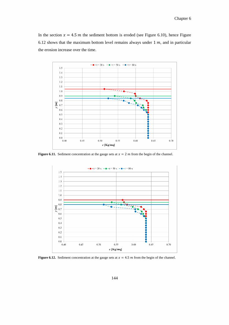
Chapter 6

144

In the section the sediment bottom is eroded (see Figure 6.10), hence Figure

6.12 shows that the maximum bottom level remains always under , and in particular

the erosion increase over the time.



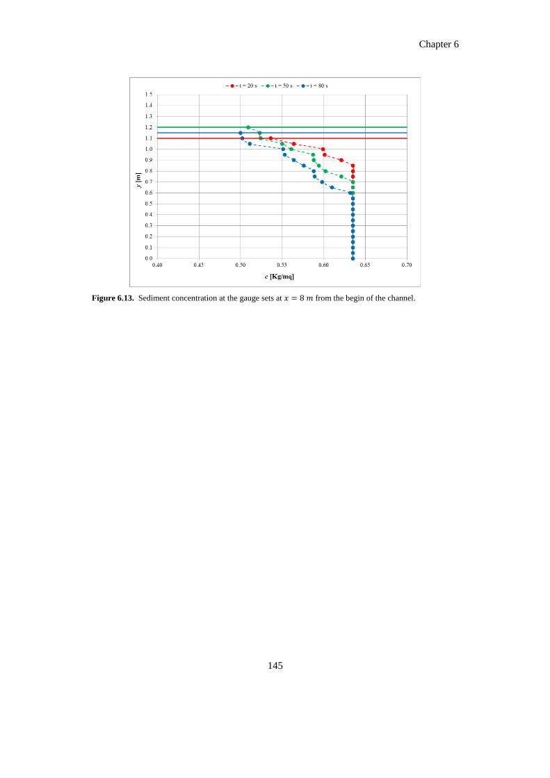
Chapter 6

145


CHAPTER 7

CONCLUSIONS AND FUTURE WORK.

The main objective of this thesis work was to develop a tool that can represent wave run-

up and overtopping together with beach reshaping during storms. A two-dimensional

numerical model based on the Reynolds Averaged Navier–Stokes equations (RANS),

called IH-2VOF, was selected. This numerical model was used to study the wave-

structure interaction and then the new equations for the representation of the sediment

transport were introduced.

More than 90 numerical simulations with IH-2VOF model were carried out in order to

analyze the flow characteristics (velocities and layer thicknesses) on a dike crest. The

numerical data, derived by this analysis, allowed to perform a systematic investigation,

which may be useful to extend the existing theoretical approach and provide criteria for

design application.

First, in order to verify the numerical simulations, selected numerical results were

compared against experimental data and consolidated theoretical formulae. In particular,

the wave reflection coefficients calculated numerically for each test was compared with

the experimental results obtained by Zanuttigh et al. (2006). The numerical values of

appear to be slightly greater than the experimental values. However, the numerical trends

show two key issues in agreement with the physical process: the greater the submergence

and/or the lower the wave height, the lower the reflection.

As regards the discharge, the numerical values were compared with the theoretical

formulae proposed by Eurotop 2007. Both for emerged and zero freeboard cases, the

theoretical discharge was well represented by the numerical one. Instead, for submerged

cases, the theoretical overflow discharge is well represented by the numerical one,

whereas the theoretical overtopping discharge is overestimated. However, this contribute

is very small and so it does not affect too much the total results.

Chapter 7

147

The effects of the structure design parameters (i.e. slopes and submergence) on the trend

of both depths and velocities over the crest were in-depth investigated. First it was found

that the seaward/landward slope does not significantly affect the evolution of the flow

depth and velocity over the dike crest whereas the most important parameter is the

relative submergence. Wave heights decrease and flow velocities increase while waves

travel over the crest. In particular, by increasing the submergence, the wave height decay

is less marked and it completely disappears when , whereas the increase of

the velocity start from about the middle of the crest of the structure and however are very

modest. Besides, an appropriate curve able to fit the variation of the wave height/velocity

over the dike crest were found. Both for the wave height and for the wave velocity

different fitting coefficients were determined on the basis of the submergence and of the

significant wave height. The results show that by keeping in constant the submergence,

the wave height decay tends to decrease, almost halved, when the significant wave height

increases. Similarly, the numerical results show that the wave height decay increases

with increasing the submergence when the significant wave height is constant.

These conclusions can be very important in terms of design criteria. In particular, by

considering that climate change might cause sea level rise and the increase of the

intensity of storms, an increasing of the risk of flooding of low lying areas, an accelerate

erosion of exposed soft beach and a damage to existing coastal protection structures may

occur. The results obtained in this thesis work (in particular reported in Chapter 4) could

be taken into consideration for the upgrade of the structures.

In this context it is also important to predict the dimensionless decay coefficient in

order to understand the rate of decay of the wave height on the dike crest. Hence the

eventual dependence of the decay coefficient on the characteristics of the structure and/or

wave attack was investigated. In particular, an equation describing the trend of the

dimensionless coefficient for the wave height was derived. By this way it is possible

to predict the decay coefficient that controls the decrease of the wave height over the dike

crest.

Chapter 7

148

The second part of this thesis work was focused on further developing the numerical

model for sediment transport, aiming at representing beach erosion while waves run-up

and overtop the sea banks during storms. Balance equations for the average mass,

momentum and energy for the two phases are phrased in terms of concentration-weighted

(Favre averaged) velocities. Closures for the correlations between fluctuations in

concentration and particle velocities are based on those for collisional grain flow.

The new model allows us to calculate sediment fluxes everywhere in the water column

together with the sediment concentration. Moreover it is possible to model the bed

profile evolution.

Two different tests were performed under low-intensity regular waves with an

homogeneous layer of sand on the bottom of a channel whose length is about half the

tested wave length. The only difference between the two tests is that in the first one the

landward (right) boundary was set as an open boundary, whereas, in the second one, the

right boundary was set as a closed boundary. The change of boundary conditions affects

the numerical model response as it can be observed from the erosion-deposition pattern.

When the landward boundary is an open boundary, erosion occurs in the first half of the

channel (within L/4 from the wave-maker) and the deposition in the second half (between

L/4 and L/2). When the landward boundary is set as a closed boundary instead, the

erosion area occurs in the middle of the channel, i.e. in correspondence with the antinode

point (L/4). In the second half of the numerical domain a strong deposition of the

sediment occurs because of the closing wall. Another important difference is that in the

first case, the sediment mass tends to decrease over the time because the landward

boundary is open and the sand can get out from the numerical domain, whereas in the

second case the sediment mass is trapped inside the channel and therefore erosion and

accumulation patterns appear to be more marked in time.

Further work should be done to

validate the sediment transport model on a quantitative basis, considering

experimental and theoretical results available in the literature;

Chapter 7

149

examine the robustness of the model to reproduce different wave attacks and

sediment configurations, including the representation of more complex sediment

geometries inside the numerical code developed so far;

analyse beach reshaping during storms and compare to real prototype data for

assessing beach retreat and increase hydraulic vulnerability.

REFERENCES

Alsina, J.M., Baldock, T.E., Hughes, M.G., Weir, F., Sierra, J.P., 2005.

Sediment transport numerical modelling in the swash zone. In: Proceedings of Coastal

Dynamics ‘05, Barcelona, ASCE.

Antuono, M., Brocchini, M., Grosso, G., 2007. Integral properties of the swash

zone and averaging. Part 3. Longshore shoreline boundary conditions for wave-

averaged nearshore circulation models. Journal of Fluid Mechanics 573, 399–415.

Archetti, R., Brocchini, M., 2002. An integral swash zone model with friction:

an experimental and numerical investigation. Coastal Engineering 45, 89–110.

Asano, T., 1990. Two-phase flow model on oscillatory sheet-flow. In:

Proceedings of the 22nd ICCE, Delft, Netherlands, pp. 2372–2384.

Asano, T., 1994. Swash motion due to obliquely incident waves. In: Proceedings

of the 24th Coastal Engineering conference, ASCE, October 23–38, Kobe, Japan, pp. 27–

41.

Baba, Y., Camenen, B., 2008. Importance of the swash longshore sediment

transport in morphodynamic models. Coastal Sediments ’07, ASCE, pp. 1938–1946.

Bagnold, R.A., 1963. Mechanics of marine sedimentation. In: Hill, M.N. (Ed.),

The Sea. Wiley-Interscience, New York, pp. 507–528.

Bagnold, R.A., 1966. An Approach to the Sediment Transport Problem from

General Physics. US Geological Survey, Washington, DC, 37pp.

Bailard, J.A., 1981. An energetics total load sediment transport model for a

plane sloping beach. Journal of Geophysical Research 86 (C11), 938–954.

Bakhtyar, R., Yeganeh-Bakhtiary, A., Ghaheri, A., 2007. Numerical

simulation of wave breaking and wave run-up in nearshore. International Conference on

Violent Flow, 20–22 November 2007, Fukuoka, Japan.

Bakhtyar, R., Ghaheri, A., Yeganeh-Bakhtiary, A., Baldock, T.E., 2008.

Longshore sediment transport estimation using fuzzy inference system. Applied Ocean

Research (in press).

Bakhtyar, R., Barry, D.A., Yeganeh-Bakhtiary, A., Ghaheri, A., 2009.

Numerical simulation of surf-swash zone motions and turbulent flow. Advances in Water

Resources 32, 250–263.

Chapter 7

151

Baldock, T.E., Holmes, P., 1997. Swash hydrodynamics on a steep beach.

Coastal Dynamics Conference, ASCE, Plymouth, UK, pp. 784–793.

Baldock, T.E., Huntley, D.A., 2002. Long wave forcing by the breaking of

random gravity waves on a beach. Proceedings of Royal Society of London A 458, 2177–

2201.

Baldock, T.E., Hughes, M.G., Day, K., Louys, J., 2005. Swash overtopping and

sediment overwash on a truncated beach. Coastal Engineering 52, 633–645.

Battjes, J. A., 1974. Computation of set-up, longshore currents, run-up and

overtopping due to wind –generated waves. Report 74-2. Committee on Hydraulics. Dept.

Of Civil Engineering, Delf University of Technology.

Bayram, A., Larson, M., Miller, H.C., Kraus, N.C., 2001. Cross-shore

distribution of longshore sediment transport: comparison between predictive formulas

and field measurements. Coastal Engineering 44, 79–99.

Bijker, E.W., 1971. Longshore transport computations. Journal of the

Waterways, Harbors and Coastal Engineering Division, ASCE 97 (4), 687–703.

Bocquet, L., Losert, W., Schalk, D., Lubensky, T. C. & Gollub, J. P., 2001

Granular shear flow dynamics and forces: experiment and continuum theory. Phys. Rev.

E65, 011307.

Bosman, G., van der Meer, J. W., Hoffmans, G., Schuttrumpf, H., and

Verhagen, H., 2008. Individual overtopping events at dikes. Proc., 31st Int. Conf.

Coastal Engineering, Vol. 4, ASCE, Reston, Va., 2944–2956.

Bradford, S.F., 2000. Numerical simulation of surf zone dynamics. Journal of

Waterway, Port, Coastal, and Ocean Engineering, ASCE 126 (1), 1–13.

Brocchini, M., Peregrine, D.H., 1995. Flow properties of the swash zone.

Proceedings of Coastal Dynamics’95, ASCE, 221-232.

Brocchini, M., Peregrine, D.H., 1996. Integral flow properties of the swash

zone and averaging. Journal of Fluid Mechanics 317, 241–273.

Calantoni, J., Puleo, J.A., Holland, K.T., 2006. Simulation of sediment motions

using a discrete particle model in the inner surf and swash-zones. Continental Shelf

Research 26, 610–621.

Carrier, G.F., Greenspan, H.P., 1958. Water waves of finite amplitude on a

sloping beach. Journal of Fluid Mechanics 4 (1), 97–109.

Chapter 7

152

Champagne, F.H., Harris, V.G., Coorsin, S., 1970. Experiments on nearly

homogeneous turbulent shear flow. Journal of Fluid Mechanics, 41: 81-139.

Chapman, S. & Cowling, T. G., 1970 The mathematical theory of non-

uniform gases. 3rd edn. Cambridge University Press.

Chopakatla1, S.C., Lippmann, T.C., Richardson, J.H., 2008. Field

verification of a computational fluid dynamics model for wave transformation and

breaking in the surf zone. Journal of Water way, Port, Coastal, and Ocean Engineering,

ASCE 134 (2), 71–80.

Christensen, E.D., Deigaard, R., 2001. Large eddy simulation of breaking

waves. Coastal Engineering 42, 53–86.

Christensen, E.D., 2006. Large eddy simulation of spilling and plunging

breakers. Coastal Engineering 53, 463–485.

CLASH, 2004. Crest Level Assessment of coastal Structures by full scale

monitoring, neural network prediction and Hazard analysis on permissible wave

overtopping. EC-contract EVK3-CT-2001-00058. www.clash-eu.org.

Crowe, C.T. (Ed.), 2006. Multiphase Flow Handbook. Taylor and Francis, Boca

Raton.

Cundall, P.A., Strack, O.D., 1979. A discrete numerical model for granular

assembles. Geotechnique 29 (1), 47–65.

Dalrymple, R.A., Gómez-Gesteira M., Rogers B.D., Panizzo A., Zou S.,

Crespo A.J.C., Cuomo G., M. Narayanaswamy, 2009. Smoothed Particle

Hydrodynamics for Water Waves, in Advances in Numerical Simulation of Nonlinear

Waves Shi F., Q.Ma, ed., World Scientific Press, ISBN 981-283-649-7.

Davies, A.G., Ribberink, J.S., Temperville, A., Zyserman, J.A., 1997.

Comparisons between sediment transport models and observations made in wave and

current flows above plane beds. Coastal Engineering 31 (1–4), 163–198.

Dodd, N., 1998. A numerical model of wave run-up, overtopping and

regeneration. Journal of Waterway, Port, Coastal, and Ocean Engineering, ASCE 124

(2), 73–81.

Dong, P., Zhang, K., 1999. Two-phase flow modeling of sediment motions in

oscillatory sheet flow. Coastal Engineering 36, 87–109.

Chapter 7

153

Drake, T.G., Calantoni, J., 2001. Discrete particle model for sheet flow

sediment transport in the nearshore. Journal of Geophysical Research 106 (C9), 19859–

19868.

Drago, M., Iovenitti, L., 1995. The modelling of plunging breakers by the

introduction of a K-l turbulence closure model. In: Proceedings of Coastal Dynamics,

ASCE, pp. 317–328.

Drew, D. A., 1976 Production and dissipation of energy in the turbulent flow of a

particle–fluid mixture, with some results on drag reduction. J. Appl. Mech. 43, 543–547.

Elfrink, B., Baldock, T.E., 2002. Hydrodynamics and sediment transport in the

swash zone: a review and perspectives. Coastal Engineering 45, 149–167.

Elghobashi, S. E. & Abou-Arab, T. W., 1983. A two-equation turbulence model

for two-phase flows. Phys. Fluids 26, 931–938.

EUROSION, European Union Project ENV.B.3-SER-2001-0030, Reports

Online, Living with coastal erosion in Europe: sediment and space for sustainability, Part

1 – Major Findings and Policy Recommendations of the Eurosion project,

www.eurosion.org.

EurOtop, 2007. European Manual for the Assessment of Wave Overtopping. T.

Pullen, N.W.H. Allsop, T. Bruce, A. Kortenhaus, H. Schüttrumpf and J.W. van der Meer.

At: www.overtopping-manual.com.

Favre, A., 1965. Equations des gaz turbulent compressible. J. Méc. 4, 361–390.

Frijlink,H.C., 1952. Discussion des formules de debit solide de Kalinske,

Einstein et Meyer-Peter et Mueller compte tenue des mesures recentes de transport dans

les rivieres Neerlandaises. 2me Journal Hydraulique Societe Hydraulique de France,

Grenoble (in French), pp.98–103.

Fuhrman,D.R., Madsen, P.A.,2008. Simulation of non-linear wave run-up with

a high-order Boussinesq model. Coastal Engineering 55, 139–154.

Garcia, N., Lara, J.L., Losada, I.J., 2004a. 2-D numerical analysis of near-field

flow at low-crested breakwaters. Coastal Engineering 51 (10), 991–1020.

Garcia, N., Lara, J.L., Lomonaco, P., Losada, I.J., 2004b. Flow at low-crested

breakwaters under breaking conditions. Proceedings of the 29th International Conference

on Coastal Engineering. Word Scientific, pp. 4240-4252.

Chapter 7

154

Gotoh,H., Sakai,T., 1997. Numerical simulation of sheet flow as granular

materials. Journal of Waterway, Port, Coastal, and Ocean Engineering 123(6),329–336.

Guanche, R., I.J. Losada and J.L. Lara., 2009. Numerical analysis of wave

loads for coastal structure stability, Coastal Engineering, ELSEVIER, vol. 56, 543-558

Guard, P.A., Baldock,T.E., 2007. The influence of seaward boundary conditions

on swash zone hydrodynamics. Coastal Engineering 54, 321–331.

Higuera, P., Lara, J.L., Losada, I.J., 2013. Realistic wave generation and

active wave absorption for Navier–Stokes models. Application to OpenFOAM. Coastal

Engineering.

Higuera, P., Lara, J.L., Losada, I.J., 2013. Simulating Coastal Engineering

Processes with OpenFOAM. Coastal Engineering.

Hirt, C.W., Nichols, B.D., 1981. Volume of fluid (VOF) method for the dynamics

of free boundaries. Journal of Computational Physics 39, 201–225.

Hoffmann, M. et al., 2008. Conservation planning and the IUCN Red List.

Endangered Species Research 6, 113–125.

Hsu, T.-J., 2002. A two-phase flow approach for sediment transport. PhD thesis,

University, Ithaca, NY, USA.

Hsu, T.-J., Sakakiyama, T., Liu, P.L.-F., 2002. A numerical model for wave

motions and turbulence flows in front of a composite breakwater. Coastal

Engineering, 46: 25-50.

Hsu, T.-J., Jenkins, J.T., Liu, P.L.-F., 2003. On two-phase sediment transport:

dilute flow. Journal of Geophysical Research 108, 3057.

Hsu, T., Jenkins, J.T., Liu, P.L.-F., 2004. On two-phase sediment transport

sheet flow of massive particles. Proceedings of the Royal Society of London, Seriees A

460, 2223–2250.

Hsu, T.-J., and B. Raubenheimer, 2006. .A numerical and field study on inner-

surf and swash sediment transport, Cont. Shelf. Res., 26, 589-598.

Hu, K., Mingham, C.G., Causon, D.M., 2000. Numerical simulations of wave

overtopping of coastal structures using the non-linear shallow water wave equations.

Coastal Engineering 41, 346–365.

Hughes, M.G., Masselink, G., Brander, R.W., 1997. Flow velocity and

sediment transport in the swash zone of a steep beach. Marine Geology 138, 91–103.

Chapter 7

155

Hughes, M.G., Baldock, T.E., 2004. Eulerian flow velocities in the swash zone:

field data and model predictions. Journal of Geophysical Research 109, C08009.

Hughes, S.A., N.C. Nadal, 2009. Laboratory study of combined wave

overtopping and storm surge overflow of a levee. Coastal Engineering, 56, 244-259.

Hughes, S, C. Thornton, J.W. van der Meer and B. Scholl, 2012.

Improvements in describing wave overtopping processes. ASCE, Proc. ICCE 2012,

Santander, Spain.

Hunt, A., 1959. Design of seawalls and breakwaters. Journal of the Waterways

and Harbors Division. ASCE, pp. 123– 152.

Jenkins, J. T. & Savage, S. B., 1983. A theory for the rapid flow of identical,

smooth, nearly elastic particles. J. Fluid Mech. 370, 29–52.

Jenkins, J. T., Cundall, P. A. & Ishibashi, I., 1989. Micromechanics modeling

of granular material. In Powders and grains (ed. J. Biarez & R. Gourves), pp. 257–264.

Rotterdam: Balkema.

Jenkins, J. T. & Hanes, D. M., 1998 Collisional sheet flows of sediment driven

by a turbulent fluid. J. Fluid Mech. 370, 29–52.

Jensen, A., Pedersen, G.K., Wood, D.J., 2003. An experimental study of wave

run-up at a steep beach. Journal of Fluid Mechanics 486, 161–188.

Kamphuis, J.W., 1991. Alongshore sediment transport rate distribution. In:

Coastal Sediments ‘91, ASCE, pp. 170–183.

Kamphuis, J.W., 2002. Alongshore transport of sand, Proceedings of the 28th

Coastal Engineering Conference, ASCE, in press.

Karambas, T.V., Koutitas, C., 2002. Surf and swash zone morphology evolution

induced by nonlinear waves. Journal of Waterway, Port, Coastal, and Ocean Engineering,

ASCE 128 (3), 101–142.

Karambas, T.V., 2003. Modelling of infiltration–exfiltration effects of cross-

shore sediment transport in the swash zone. Coastal Engineering Journal 45, 63–82.

Karambas, T.V., 2006. Prediction of sediment transport in the swash zone by

using a nonlinear wave model. Continental Shelf Research 26, 599–609.

Karunarathna, H., Chadwick, A., Lawrence, J., 2005. Numerical experiments

of swash oscillations on steep and gentle beaches. Coastal Engineering 52, 497–511.

Chapter 7

156

Kennedy, A.B., Chen, Q., Kirby, J., Dalrymple, R.A., 2000. Boussinesq

modeling of wave transformation, breaking, and run-up. I: 1D. Journal of Waterway,

Port, Coastal, and Ocean Engineering, ASCE 126 (1), 39–47.

Kirby, J.T., 2003. Boussinesq models and applications to nearshore wave

propagation, surf zone processes and wave-induced currents. In: Lakhan, C. (Ed.),

Advances in Coastal Engineering. Elsevier, Amsterdam.

Kobayashi, N., Seo, S.N., 1985. Fluid and sediment interaction over a plan bed.

Journal of Hydraulic Engineering 111 (6), 903–921.

Kobayashi, N., De Silvia, G.S., Watson, K.D., 1989. Wave transformation and

swash oscillation on gentle and steep slopes. Journal of Geophysical Research 94 (C1),

951–966.

Kobayashi, N., Poff, M.T., 1994. Numerical model RBREAK2 for random waves

on impermeable coastal structures and beaches. Research Report No. CACR-94-12,

Center for Applied Coastal Research, Department of Civil Engineering, University of

Delaware, Newark, 325pp.

Kobayashi, N., Agarwal,A., Johnson,B.D., 2007. Longshore current and

sediment transport on beaches. Journal of Waterway, Port, Coastal, andOcean

Engineering, ASCE133(4),296–304.

Komar, P.D., Inman, D.L., 1970. Longshore sand transport on beaches. Journal

of Geophysical Research 75(30), 5514–5527.

Komar, P.D., 1998. Beach processes and sedimentation (2nd edition). Prentice-

Hall, New Jersey, 545 p.

Koshizuka, S., Go, S., Oka, Y., Tanizawa, K., 2004. Numerical analysis of a

two-dimensional experiment of shipping water on deck using a particle method.

Proceedings of ASME HTFED’04.

Kothe, D.B., Mjolsness, R.C., Torrey, M.D., 1991. RIPPLE: a computer

program for incompressible flows with free surfaces, Los Alamos National Laboratory.

Kumar, V.S., Anand, N.M., Chandramohan,P., Naik, G.N., 2003. Longshore

sediment transport rate – measurement and estimation, central west coast of India.

Coastal Engineering 48,95–109.

Chapter 7

157

Lara, J.L., Losada, I.J., Liu, P.L.-F., 2006. Breaking waves over a mild gravel

slope: experimental and numerical analysis. Journal of Geophysical Research, AGU,

Vol. 111, C11019; doi: 10-1029/2005 JC003374.

Lara J.L., Losada I.J., R. Guanche, 2008. Wave interaction with low-mound

breakwater using a rans model. Ocean Engineering, 56, 543-558.

Lara, J.L., Ruju, A. and Losada, I.J., 2011. Reynolds Averaged Navier-Stokes

modelling of long waves induced by a transient wave group on a beach. Proceedings of

the Royal Society A, vol. 467, 1215-1242.

Larson, M., Kubota,S., Erikson,L., 2004. Swash-zone sediment transport and

foreshore evolution: field experiment sand mathematical modeling. Marine Geology 212

(1–4), 61–80.

Lemos, C.M., 1992. Wave breaking. Springer-Verlag, New York, USA.

Leont’yev, I.O., 1999. Modelling of morphological changes due to coastal

structures. Coastal Engineering 38,143–166.

Lin, P., 1998. Numerical modeling of breaking waves. Ph.D. Thesis, Cornell

University.

Lin, P., Liu, P.L.-F., 1998a. A numerical study of breaking wave in the surf zone.

Journal of Fluid Mechanics 359, 239–264.

Lin, P., Liu, P.L.-F., 1998b. Turbulence transport, vorticity dynamics, and

solute mixing under plunging breaking waves in surf zone. Journal of Geophysical

Research 103, 15677–15694.

Lin, P., Liu, P.L.-F., 1999. Internal wave maker for Navier-Stokes equations

models. Journal of Waterway, Port, Coastal, and Ocean Engineering, ASCE 125, 207–

215.

Liu, P.L.-F., Lin, P., 1997. A numerical model for breaking waves: the volume of

fluid method. Research Report No. CACR-97-02, Center for Applied Coastal Research,

Ocean Engineering Laboratory, University of Delaware, Newark, DE.

Liu, P.L.-F., Lin, P., Chang, K.-A., Sakakiyama, T., 1999. Numerical

modeling of wave interaction with porous structures. J. Waterw., Port, Coast., and Ocean

Eng., ASCE 125 (6), 322 – 330.

Liu, H., Sato, S., 2006. A two-phase flow model for asymmetric sheet flow

conditions. Coastal Engineering 53, 825–843.

Chapter 7

158

Losada I.J., 2003. Advances in modeling the effects of permeable and reflective

structures on waves and nearshore flows. In: Chris Lakhan, V. (Ed.), Advances in

Coastal Modeling. Elsevier Oceanography Series, vol. 67.

Losada, I.J., Lara, J.L., Christensen, E.D., Garcia, N., 2005. Breaking

process, velocities and turbulence intensity around low crested structures. Coastal

Engineering, “DELOS” Special Issue.

Losada, I.J., J.L. Lara, R. Guanche and J.M. Gonzalez-Ondina, 2008.

Numerical analysis of wave overtopping of rubble mound breakwaters, Coastal

Engineering, ELSEVIER, 55(1), 47-62 (2008)

Lynett, P., Wu, T.-R., Liu, P.L.-F., 2002. Modelling wave run-up with depth-

integrated equations. Coastal Engineering 46, 89–107.

Lynett, P., Liu, P.L.-F., 2004. A two-layer approach to water wave modeling.

Proceedings of the Royal Society of London, Series A 460, 2637–2669.

Lynett, P., 2006. Nearshore modeling using high-order Boussinesq equations.

Journal of Waterway, Port, Coastal, and Ocean Engineering, ASCE 132 (5), 348–357.

McTigue, D. F., 1981. Mixture theory for suspended sediment transport. J.

Hydraul. Div. ASCE 107, 659–673.

Madsen, O.S., 1991. Mechanics of cohesionless sediment transport in coastal

waters. Coastal Sediments ‘91. ASCE, Seattle, Washington, pp. 15–27.

Madsen, O.S., 1993. Sediment transport on the shelf. In: Proceedings of the

Sediment Transport Workshop DRP TA1, 8–9 June. CERC, Vicksburg, MS.

Madsen, P.A., Sørensen, O.R., Schaffer, H.A., 1997b. Surf zone dynamics

simulated by a Boussinesq type model. Part II. Surf beat and swash oscillations for wave

groups and irregular waves. Coastal Engineering 32, 289–319.

Masselink, G., Hughes, M., 1998. Field investigation of sediment transport in

the swash zone. Continental Shelf Research 18 (10), 1179–1199.

Masselink, G., Evans, D., Hughes, M.G., Russell, P., 2005. Suspended

sediment transport in the swash zone of a dissipative beach. Marine Geology 216, 169–

189.

Meyer-Peter, E., Muller, R., 1948. Formulas for bed-load transport. In:

Proceedings of the 3rd Meeting of the International Association for Hydraulic Research,

Stockholm, Sweden, pp. 39–64.

Chapter 7

159

Miles, L., Newton, A. C., Defries, R., Ravilious, C., May, I., Blyth, S., Kapos,

V., Gordon, J., 2006. A global overview of the conservation status of tropical dry

forests. Journal of Biogeography 33: 491-505.

Nakayama, A., Kuwahara, F., 1999. A macroscopic turbulence model for

flow in a porous medium. Journal of Fluids Engineering, 121: 427-433.

Nield, D.A., Bejan, A., 1999. Convection in porous media. 2nd

edition, Springer-

Verlag, New York, USA.

Nielsen, P., 1990. Tidal dynamics of the water table in beaches. Water Resources

Research 26 (9), 2127–2134.

Nielsen, P., 2002. Shear stress and sediment transport calculations for swash

zone modeling. Coastal Engineering 45, 53–60.

Nielsen, K.B., Mayer, S., 2004. Numerical prediction of green water incidents.

Ocean Engineering 31 (3–4), 363–399.

Ono, M., Deguchi, I., Sawaragi, T., 1996. Numerical modeling of sediment

transport for various mode. In: Proceedings of 25th International Conference on Coastal

Engineering. ASCE, New York, pp. 3888–3900.

Owen, M.W., 1980. Design of seawalls allowing for wave overtopping.

Technical Report EX-924. H.R. Wallingford, United Kingdom.

Park, J.C., Kim, M.H., Miyata, H., 1999. Fully non-linear free-surface

simulations by a 3D viscous numerical wave tank. International Journal for Numerical

Methods in Fluids 29 (6), 685–703.

Pedrozo-Acuña, A., Simmonds, D.J., Otta, A.K., Chadwick, A.J., 2006. On

the cross- shore profile change of gravel beaches. Coastal Engineering 53(4), 335–347.

Pedrozo-Acuña, A., Simmonds, D.J., Chadwick, A.J., Silva, R., 2007. A

numerical- empirical approach for evaluating morphodynamic processes on gravel and

mixed sand-gravel beaches. Marine Geology 241, 1–18.

Pilkey, O. H., Hume, T., 2001. Coastal research – the shoreline erosion

problem: lessons from the past. Water and Atmosphere, 9(2), National Institute of Water

and Atmosphere, New Zealand. [http://www.niwa.cri.nz]

Pope, S.B., 2000. Turbulent Flows. University Press, Cambridge, UK,771pp.

Chapter 7

160

Puleo, J.A., Slinn, D.N., Holland, K.T., Smith, E., Webb, B.M., 2002.

Numerical modeling of swash zone hydrodynamics. In: Proceedings of the American

Society of Civil Engineers, Cardiff, Wales, UK.

Puleo, J.A., Holland, K.T., Plant, N., Slinn, D.N., Hanes, D.M., 2003. Fluid

acceleration effects on suspended sediment transport in the swash zone. Journal of

Geophysical Research 108 (C11), 3350, 10.1029/2003JC001943.

Rakha, K.A., Deigaard, R., Brøker, I., 1997. A phase-resolving cross shore

sediment transport model for beach profile evolution. Coastal Engineering 31, 231–261.

Raubenheimer, B., 2002. Observations and predictions of fluid velocities in the

surf and swash zones. Journal of Geophysical Research 107 (C11), 3190.

Ribberink, J.S., Al-Salem, A.A., 1995. Sheet flow and suspension of sand in

oscillatory boundary layers. Coastal Engineering 25, 205–225.

Richardson, J. F., Zaki, W. N., 1954. Sedimentation and fluidization. Part 1.

Trans. IChE 32, 35–53.

Rodi, W., 1980. Turbulence models and their application in hydraulics – a state-

of-the-art review. IAHR Publication.

Schüttrumpf, H., 2001. Wellenüberlaufströmung bei Seedeichen –

Experimentelle und Theoretische Untersuchungen. PhD-Thesis.

Schüttrumpf, H., van Gent, M.R., 2003. Wave overtopping at seadikes.

Proceedings of Coastal Structures, '03. American Society of Civil Engineers, pp. 431–

443.

Schüttrumpf H., H. Oumeraci, 2005. Layer thicknesses and velocities of wave

overtopping flow at sea dikes. Coastal Engineering, 52 (6), 473-495.

Shen, M.C. and Meyer, R.E., 1963. Climb of a bore on a beach. Part 3. Runup.

J. Fluid Mech., 16: 113-125.

Shiach, J.B., Mingham, C.G., Ingram, D.M., Bruce, T., 2004. The

applicability of the shallow water equations for modelling violent wave overtopping.

Coastal Engineering 51 (1), 1–15.

Shih, T.H., Zhu, J., Lumley, J.L., 1996. Calculation of wall-bounded

complex flows and free shear flows. International Journal for Numerical Methods in

Fluids, 23: 1133-1144.

Chapter 7

161

Shore Protection Manual,1984. USArmy Engineer Waterways Experiment

Station, US Government Printing Office, Washington, DC. Shen, M.C., Meyer, R.E.,

1963. Climb of a bore on a beach: Part3, run-up. Journal of Fluid Mechanics 16(8),113–

125.

Shen, Y.M., Ng, C.O., Zheng, Y.H., 2004. Simulation of wave propagation over

a submerged bar using the VOF method with a two-equation k-eps turbulence modeling.

Ocean Engineering 31(1), 87–95.

Shields, A.,1936. An wending der Ahnlichkeits Mechanik und der Turbulenz-

forschung auf die Geschiebe Bewegung, 26. Mitteilungen Preuss. Versuchan- stalt fur

Wasserbau and Schiffbau, Berlin, 26pp.

Sitanggang, K., Lynett, P., 2005. Parallel computation of a highly nonlinear

Boussinesq equation model through domain decomposition. International Journal for

Numerical Methods in Fluids 49 (1), 57–74.

Smith, E.R.,Ebersole,B.A.,Wang,P.,2004. Dependence of total longshore

sediment transport rate son incident wave parameter sand breaker type. Technical Report

ERDC/CHLCHETN-IV-62, USArmy Engineer Research and Development Center,

Vicksburg, MS.

Sørensen, O.R., Schaffer, H.A., Sørensen, L.S., 2004. Boussinesq-type

modelling using an unstructured finite element technique. Coastal Engineering 50, 181–

198.

Sumer, B. M., Kozakiewicz, A., Fredsoe, J. & Deigaard, R., 1996. Velocity

and concentration profiles in sheet-flow layer of movable bed. J. Hydraul. Engng 122,

549–558.

Tajima, Y., 2004. Waves, currents, and sediment transport in the surf zone along

long, straight beaches. Ph.D. Thesis, Massachusetts Institute of Technology, 313 pp.

Tautenhain, E., 1981. Der Wellenu¨berlauf an Seedeichen unter

Beru¨cksichtigung des Wellenauflaufs. Mitteilungen des Franzius- Instituts. H., 53, 1 –

245.

THESEUS project “Innovative technologies for safer European coasts in a

changing climate”, FP7.2009-1, Contract 244104, is gratefully acknowledged.

Torquato, S., 1995. Nearest-neighbor statistics for packings of hard spheres and

disks. Phys. Rev. E51, 3170–3182.

Chapter 7

162

Torres-Freyermuth, A., Lara, J.L. and Losada, I.J., 2010. Numerical

modelling of short and long-wave transformation on a barred beach. Coastal

Engineering, vol. 57, 317-330.

Van der Meer, J.W., Janssen, W., 1995. Wave run-up and wave overtopping at

dikes. In: Kabayashi, Demirbilek (Eds.),Wave Forces on Inclined and VerticalWall

Structures. American Society of Civil Engineers, pp. 1–27.

Van der Meer, J.W., Bernardini, P., Snijders,W., E. Regeling, 2006. The wave

overtopping simulator. Proceedings of the 30th International Conference on Coastal

Engineering, vol. 5. World Scientific, 4654–4666.

Van der Meer, J. W., Steendam, G. J., de Raat, G., and Bernardini, P.,2008.

Further developments on the wave overtopping simulator. Proc., 31st Int. Conf. Coastal

Engineering, Vol. 4, ASCE, Reston, Va., 2957–2969.

Van der Meer, J.W., R. Schrijver, B. Hardeman, A. van Hoven, H. Verheij

and G.J. Steendam, 2009. Guidance on erosion resistance of inner slopes of dikes from

three years of testing with the Wave Overtopping Simulator. Proc. ICE, Breakwaters,

Marine Structures and Coastlines; Edinburgh, UK.

Van der Meer J. W., Hardeman B., Steendam S.J., Schüttrumpf H., H.

Verheij, 2010. Flow depth and velocities at crest and landward slope of a dike, in theory

and with the wave overtopping simulator. ASCE, Proc. ICCE 2010, Shanghai.

Van Wellen, E., Baldock, T., Chadwick, A.J., Simmonds, D., 2000. STRAND:

a model for longshore sediment transport in the swash zone. In: Proceedings of the 27th

International Conference on Coastal Engineering, ASCE, Sydney, pp. 3139–3150.

Van Gent, M.R., 1994. The modelling of wave action on and in coastal

structures. Coastal Engineering, 22: 311-339.

Van Gent M.R., 2002. Wave overtopping events at dikes. Proceedings of the

28th International Coastal Engineering Conference, vol. 2. World Scientific, 2203–2215.

Victor, L., J.W. van der Meer and P. Troch, 2012. Probability distribution of

individual wave overtopping volumes for smooth impermeable steep slopes with low crest

freeboards. Coastal Engineering, 64, pp.87–101.

Wassing, F., Model investigations of wave run-up on dikes carried out in the

Netherlands during the past twenty years, Proc. 6th Conf. Coastal Eng., Gainesville,

1957, p. 700-714.

Chapter 7

163

Walton Jr., T.L., Bruno, R.O., 1989. Longshore transport at a detached break

water, phase II. Journal of Coastal Research 65 (9), 667–668.

Watanabe, A., 1992. Total rate and distribution of longshore sand transport. In:

Proceedings of the 23rd Coastal Engineering Conference, ASCE, New York, pp. 2528–

2541.

Wood, D.J., Pedersen, G.K., Jensen, A., 2003. Modelling of run-up of steep

non- breaking waves. Ocean Engineering 30, 625–644.

Yeganeh-Bakhtiary, A., Gotoh, H., Sakai, T., 2000. Applicability of Euler–

Lagrange coupling multiphase-flow model to bed-load transport under high bottom

shear. Journal of Hydraulic Research 38, 389–398.

Zanuttigh B., J.W. van der Meer, Wave reflection from coastal structures in

design conditions, Coastal Engineering, 2008, 55 (10), pp. 771 – 779.

Zanuttigh, B., J.W. van der Meer, T. Bruce and S. Hughes, 2013. Statistical

characterization of extreme overtopping wave volumes. Proc. ICE 2013, Edinburgh.

Zhang, Y., Campbell, C. S., 1992 The interface between fluid-like and solid-like

behavior in two-dimensional granular flows. J. Fluid Mech. 237, 541–568.

Zhang, Q., Liu, P.L.-F., 2008. A numerical study of swash flows generated by

bores. Coastal Engineering 55 (12), 1113–1134. Zhao, Q., Armfield, S., Tanimoto, K.,

2004. Numerical simulation of breaking waves by a multi-scale turbulence model.

Coastal Engineering 51, 53–80.

Zhao, Q., S. Armfield and K. Tanimoto, 2004: Numerical simulation of

breaking waves by a multi-scale turbulence model. Coastal Engineering 51, pp. 53-80.

Zhou, J.G., Stansby, P.K., 1999. An arbitrary Lagrangian–Eulerian model with

non- hydrostatic pressure for shallow water flows. Computer Methods in Applied

Mechanics and Engineering 178, 199–214.

Documents

Settore Concorsuale di afferenza: 08/A1 Settore ...amsdottorato.unibo.it/6626/1/raosa_andrea_natalia_tesi.pdf · 7 Figure 4.13. Wave height trend on the dike crest for tests characterized