Setting Risk Priorities: A Formal Model - Social and …sds.hss.cmu.edu/risk/articles/Risk032.pdfSetting Risk Priorities 341 has at least interval-scale properties. As mentioned, the

Risk Analysis, Vol. 20, No. 3, 2000

339

0272-4332/00/0600-0339$16.00/1 © 2000 Society for Risk Analysis

Risk032

Setting Risk Priorities: A Formal Model

Jun Long

1

and Baruch Fischhoff

1,2

*

This article presents a model designed to capture the major aspects of setting prioritiesamong risks, a common task in government and industry. The model has both

design

features,under the control of the rankers (e.g., how success is evaluated), and

context

features, proper-ties of the situations that they are trying to understand (e.g., how quickly uncertainty can bereduced). The model is demonstrated in terms of two extreme ranking strategies. The first,

se-quential risk ranking

, devotes all its resources, in a given period, to learning more about a sin-gle risk, and its place in the overall ranking. This strategy characterizes the process for a soci-ety (or organization or individual) that throws itself completely into dealing with one riskafter another. The other extreme strategy,

simultaneous risk

ranking

, spreads available re-sources equally across all risks. It characterizes the most methodical of ranking exercises.Given ample ranking resources, simultaneous risk ranking will eventually provide an accu-rate set of priorities, whereas sequential ranking might never get to some risks. Resourceconstraints, however, may prevent simultaneous rankers from examining any risk very thor-oughly. The model is intended to clarify the nature of ranking tasks, predict the efficacy of al-

ternative strategies, and improve their design.

KEY WORDS:

Risk ranking; muddling through; risk communication; comparative risk

1. INTRODUCTION

Scarce time and resources prevent individualsand societies from doing everything that they mightto reduce risks to health, safety, and environment.

(1,2)

When people face many risks, even evaluating the op-tions for risk management can be overwhelming. Onecommon strategy for coping with such overload is torank risks in terms of their magnitude. Having doneso, one can begin evaluating the options by startingwith those directed at the largest risks.

This article provides a general analytic approach

to evaluating the efficacy of alternative risk-rankingstrategies. The model can be used prescriptively, inorder to design prioritization processes. It can also beused descriptively, in order to predict the efficacy ofactual processes. Its parameters reflect both the goalsthat risk managers set for themselves and the situa-tions that confront them. Once a situation has beencharacterized in the model’s terms, one can, for ex-ample, compare the efficiency of devoting fixed re-sources to examining all members in a class of risks si-multaneously or to learning sequentially about aseries of focal risks (e.g., those nominated by thenews media for the “risk-of-the-month club”).

Setting priorities is, of course, as old (and as gen-eral) a process as making lists of personal worries.Ranking risks has gained prominence as a public pol-icy tool, in part, through the U.S. Environmental Pro-tection Agency’s (EPA’s) sustained efforts to evalu-ate its own resource allocations. In 1987, EPApublished

Unfinished Business: A Comparative As-

1

Department of Engineering and Public Policy, Carnegie MellonUniversity, Pittsburgh, PA.

2

Department of Social and Decision Sciences, Carnegie MellonUniversity, Pittsburgh, PA.

*Address correspondence to Baruch Fischhoff, Department of En-gineering & Public Policy, Department of Social and Decision Sci-ences, Carnegie Mellon University, Pittsburgh, PA 15213; [email protected]

Q1

340 Long and Fischhoff

sessment of Environmental Problems

.

(3)

In it, EPA’ssenior scientific staff divided a wide range of environ-mental and ecological risks into 31 categories. Somecategories reflected existing EPA programs or stat-utes; others were the responsibility of other agenciesor of none at all. The ranking recognized the multi-attribute character of risks, by including health, eco-logical, and welfare effects. The technical feasibilityand costs of controlling the risks were left for a laterday.

Unfinished Business

propelled a public discus-sion of risk-based priority setting.

(1)

It was followedby the EPA Science Advisory Board’s

Reducing Risks:Setting Priorities and Strategies for Environmental Pro-tection

.

(4)

In the ensuing decade, EPA sponsored astring of state, regional, and local comparative riskanalyses.

(5,6)

These efforts have generally been viewedas useful experiences, bringing together diverse indi-viduals and reaching some degree of consensus onrisk priorities. Given the need for public discourseabout the meaning of “risk,”

(7)

these encountersmight have been socially valuable, whatever progressthey made in determining the relative magnitude ofrisks. They are, in any case, but one representative ofa process that plays itself out in many places, whereregulatory agencies, industrial safety departments,public schools, hospitals, and the like decide where tofocus their attentions.

If one accepts the need for setting risk priorities,then it is important to design the process effectively.Using rankers’ time well should increase both theproduct of their labors and their willingness to investin the process. This analysis begins by offering amodel characterizing the fundamental structure ofrisk ranking. That model is then realized in the formof a simulation, designed to compute the efficacy ofalternative ranking strategies. It is used here to ex-amine several archetypal situations, chosen to cap-ture variants on the extremes of sequential and si-multaneous evaluation. The article concludes with adiscussion of the data demands for applying themodel to specific risk domains, as well as possibleelaborations.

As characterized by Lindblom

(8)

in the absenceof systematic, simultaneous ranking, prioritieschange through some form of “muddling through”;As individuals or organizations, we face some currentjumble of risks. Periodically, a specific hazard drawsour attention. After investing some resources, we un-derstand it better, possibly changing its place in theoverall risk ranking. Then, we turn our attention tothe next hazard, and the next. Over time, this sequen-tial process should gradually improve the prioritiza-

tion of the whole set. How quickly that happensshould depend on (1) the uncertainties in the situa-tion we face, (2) what we hope to get out of it, and (3)how we allocate our resources. The same factorsshould determine our success, if we try to learn aboutseveral (or all) risks at once, but must spread thesame learning resources over them.

The model presented here is designed to capturethese three elements of risk-ranking situations. Itslogic is as follows: At the beginning of a ranking pe-riod, beliefs about the magnitudes of risks are sum-marized in terms of subjective probability distribu-tions (SPDs). Their spread reflects uncertainty about(1) the expected magnitude of the adverse effectsthat each hazard can cause, and (2) the weights to as-sign to those effects, when creating an aggregate mea-sure of risk.

(10,11)

The rankers decide how to allocatetheir resources in order to learn more about one,some, or all of these risks. After that learning period,the subjective probability distributions are updatedas a function of how readily the uncertainties yield tosuch scrutiny. After completing each period, rankersevaluate the return on their investment, measured interms of the reduction in their “confusion” about therelative magnitudes of the risks. The model is imple-mented in Analytica,

3

and demonstrated here withhypothetical scenarios, meant to capture some arche-typal situations. We believe, however, that it can clar-ify the nature of some risk-ranking tasks, even with-out pursuing full computational solutions.

2. MODEL DESCRIPTION

2.1. Assumptions

For the sake of simplification, the following as-sumptions are made in the current implementation ofthe model:

1. Risks are stable over the prioritization pe-riod. The ranking process may have been ini-tiated by a perception that risks have changed(as well as by a perception that they havebeen misestimated). Whether or not that isthe case, no further changes are allowed dur-ing the ranking process.

2. The risks can be represented along a single di-mension, aggregating whatever attributesrankers deem relevant.

(11–15)

That dimension

3 Analytica Version 1.1.1, Lumina Decision Systems, Inc., 1997;http://www.lumina.com/.

Q2a

Setting Risk Priorities 341

has at least interval-scale properties. Asmentioned, the overall uncertainty regardingthe magnitude of a risk reflects the un-certainty about both how to weight the at-tributes of risk and how to characterize therisk on each relevant attribute. Thus, it is pos-sible to know risks very well (in terms of theexpected magnitudes of their effects, basedon the different attributes), but still not knowwhat to think about them (in terms of the dif-ferent trade-offs that they present across theattributes).

2.2. Model Overview

The model represents each risk by an SPD overthe risk measure. The risks are ranked according to a

ranking criterion

, representing some fractile of eachSPD (e.g., the median, 0.99). Each round of the risk-ranking process involves devoting

learning resources

to reducing uncertainties about the risks. The updat-ing process could be Bayesian (if one is designing anoptimal process) or non-Bayesian (if one is predict-ing an imperfect one). When the initial SPDs are bi-ased, the learning process will tend to correct them,perhaps increasing uncertainty. At the end of eachround, the

residual confusion

(RC) in the ranking ismeasured by the overlap in the SPDs. The critical de-sign decision is the

allocation rule

for spreading thelearning resources available for a round, across therisks.

The initial SPDs are a state of nature, with whichthe rankers must contend; so is the

uncertainty reduc-tion function

(URF), describing how quickly uncer-tainty decreases, as a function of the resources in-vested in understanding a risk. The rankers cancontrol (1) how they rank the risks (given the SPDs),(2) how they allocate those learning resources, (3)how they update their beliefs after learning, and (4)how they evaluate their RC. The next section formal-izes these two states of nature and describes four de-sign choices.

2.3. Model Parameters

2.3.1. States of Nature

Initial Estimates.

The model starts with a set ofhazards, characterized in terms of SPDs, reflectingrankers’ beliefs about the magnitudes of the risks. Asmentioned, the uncertainties may reflect both ques-tions of fact (how large each adverse effect is ex-

pected to be) and questions of value (how the effectsshould be weighted). Analytical convenience favorscharacterizing SPDs in standard terms (e.g., a normaldistribution, with specified mean and standard devia-tion). However, any form of distribution is possible inprinciple.

Initial SPDs can be biased by measurement er-rors, theoretical misconceptions, and erroneous per-ceptions of the facts.

(16–18)

A model’s specification in-cludes whether bias is suspected in the initial SPDs.

Uncertainty Reduction.

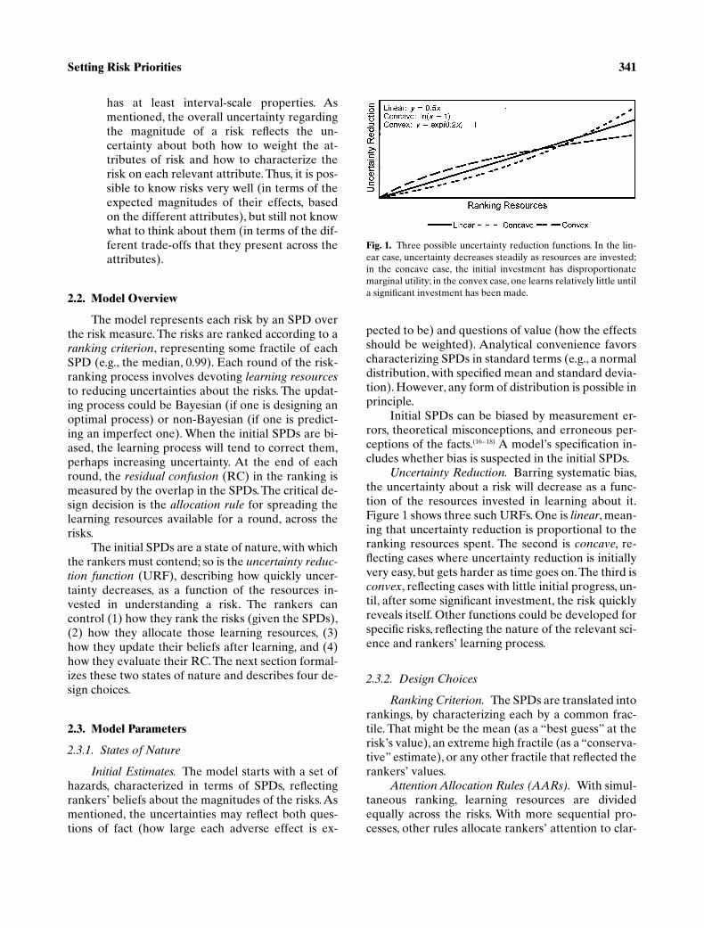
Barring systematic bias,the uncertainty about a risk will decrease as a func-tion of the resources invested in learning about it.Figure 1 shows three such URFs. One is

linear

, mean-ing that uncertainty reduction is proportional to theranking resources spent. The second is

concave

, re-flecting cases where uncertainty reduction is initiallyvery easy, but gets harder as time goes on. The third is

convex

, reflecting cases with little initial progress, un-til, after some significant investment, the risk quicklyreveals itself. Other functions could be developed forspecific risks, reflecting the nature of the relevant sci-ence and rankers’ learning process.

2.3.2. Design Choices

Ranking Criterion.

The SPDs are translated intorankings, by characterizing each by a common frac-tile. That might be the mean (as a “best guess” at therisk’s value), an extreme high fractile (as a “conserva-tive” estimate), or any other fractile that reflected therankers’ values.

Attention Allocation Rules (AARs).

With simul-taneous ranking, learning resources are dividedequally across the risks. With more sequential pro-cesses, other rules allocate rankers’ attention to clar-

Fig. 1. Three possible uncertainty reduction functions. In the lin-ear case, uncertainty decreases steadily as resources are invested;in the concave case, the initial investment has disproportionatemarginal utility; in the convex case, one learns relatively little untila significant investment has been made.


ifying particular risks.

4

A risk might be chosen atrandom (e.g., to make the selection process unpre-dictable to risk managers). Or, some special propertymight draw attention. For example, rankers might fo-cus on risks with the largest means or the largest

n

thfractiles, or with the greatest uncertainty or coeffi-cient of variation. Attention might depend on recentperformance, such as focusing on risks that have hadrecent anomalous events.

(19)

Slovic, Fischhoff, andLichtenstein

(20)

discuss the attention drawn by eventswith high “signal value,” which observers may fearsignals a change in the hazard, whose risk level needsto be reassessed. Risks with great uncertainty shouldbe particularly likely to produce such unpleasant sur-prises (and less noticed pleasant ones).

Updating Process.

Uncertainty reduction pro-ceeds by combining new information with the initialSPDs in order to get posterior SPDs. Bayesian updat-ing can be assumed, either when the ranking processis required to proceed that way or when it is expectedto do so naturally (at least to a first approximation).Given the power of Bayesian inference, our modelfocuses on it and on the use of conjoint distributions,with which updating is computationally simple. How-ever, individuals are not always Bayesians. Some-times, tiny bits of new information swing opinions; atother times, people hold tenaciously to old beliefs,even in the face of great counterevidence. The modelcan accommodate such possibilities by the simple ex-pedient of overweighting or underweighting new ev-idence, in a Bayesian calculation. Other updatingrules are also possible.

(21–23)

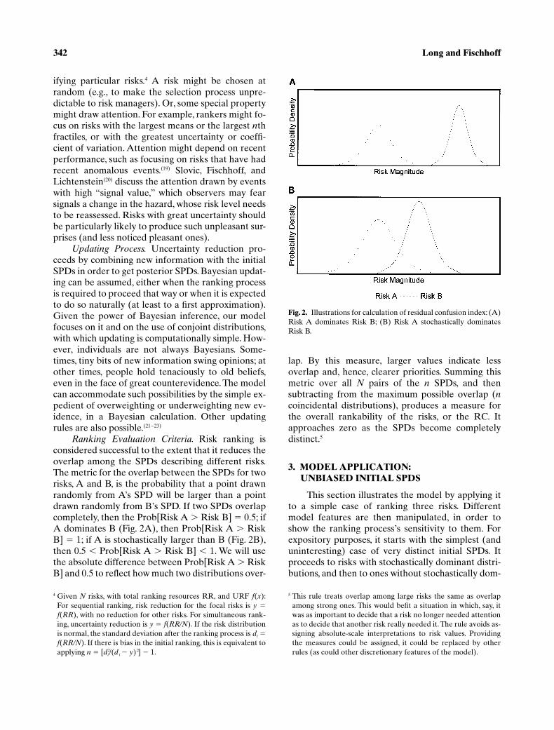
Ranking Evaluation Criteria.

Risk ranking isconsidered successful to the extent that it reduces theoverlap among the SPDs describing different risks.The metric for the overlap between the SPDs for tworisks, A and B, is the probability that a point drawnrandomly from A’s SPD will be larger than a pointdrawn randomly from B’s SPD. If two SPDs overlapcompletely, then the Prob[Risk A

�

Risk B]

�

0.5; ifA dominates B (Fig. 2A), then Prob[Risk A

�

RiskB]

�

1; if A is stochastically larger than B (Fig. 2B),then 0.5

�

Prob[Risk A

�

Risk B]

�

1. We will usethe absolute difference between Prob[Risk A

�

RiskB] and 0.5 to reflect how much two distributions over-

4 Given N risks, with total ranking resources RR, and URF f(x):For sequential ranking, risk reduction for the focal risks is y �f(RR), with no reduction for other risks. For simultaneous rank-ing, uncertainty reduction is y � f(RR/N). If the risk distributionis normal, the standard deviation after the ranking process is di �f(RR/N). If there is bias in the initial ranking, this is equivalent toapplying n � [di

2/(di � y)2] � 1.

lap. By this measure, larger values indicate lessoverlap and, hence, clearer priorities. Summing thismetric over all

N

pairs of the

n

SPDs, and thensubtracting from the maximum possible overlap (

n

coincidental distributions), produces a measure forthe overall rankability of the risks, or the RC. Itapproaches zero as the SPDs become completelydistinct.

5

3. MODEL APPLICATION:UNBIASED INITIAL SPDS

This section illustrates the model by applying itto a simple case of ranking three risks. Differentmodel features are then manipulated, in order toshow the ranking process’s sensitivity to them. Forexpository purposes, it starts with the simplest (anduninteresting) case of very distinct initial SPDs. Itproceeds to risks with stochastically dominant distri-butions, and then to ones without stochastically dom-

5 This rule treats overlap among large risks the same as overlapamong strong ones. This would befit a situation in which, say, itwas as important to decide that a risk no longer needed attentionas to decide that another risk really needed it. The rule avoids as-signing absolute-scale interpretations to risk values. Providingthe measures could be assigned, it could be replaced by otherrules (as could other discretionary features of the model).

Fig. 2. Illustrations for calculation of residual confusion index: (A)Risk A dominates Risk B; (B) Risk A stochastically dominatesRisk B.


inant SPDs. The initial SPDs are assumed here tohave no systematic bias, in the sense of being cen-tered on the true SPD. Thus, ranking should tighten,but not shift, the distributions. Section 4 allows for bi-ased initial beliefs. In such cases, information gather-ing could increase uncertainty, even as it brings therankings closer to their desired values.

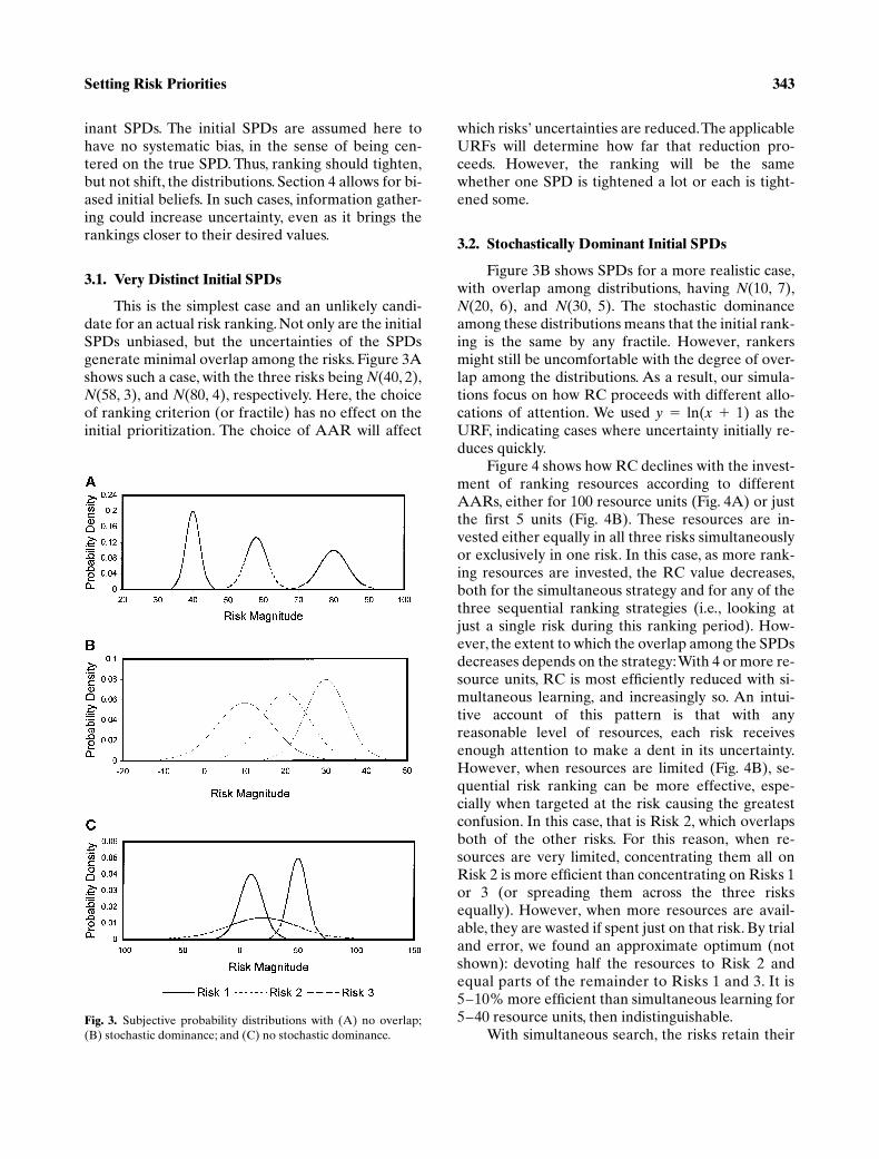
3.1. Very Distinct Initial SPDs

This is the simplest case and an unlikely candi-date for an actual risk ranking. Not only are the initialSPDs unbiased, but the uncertainties of the SPDsgenerate minimal overlap among the risks. Figure 3Ashows such a case, with the three risks being

N

(40, 2),

N

(58, 3), and

N

(80, 4), respectively. Here, the choiceof ranking criterion (or fractile) has no effect on theinitial prioritization. The choice of AAR will affect

which risks’ uncertainties are reduced. The applicableURFs will determine how far that reduction pro-ceeds. However, the ranking will be the samewhether one SPD is tightened a lot or each is tight-ened some.

3.2. Stochastically Dominant Initial SPDs

Figure 3B shows SPDs for a more realistic case,with overlap among distributions, having

N

(10, 7),

N

(20, 6), and

N

(30, 5). The stochastic dominanceamong these distributions means that the initial rank-ing is the same by any fractile. However, rankersmight still be uncomfortable with the degree of over-lap among the distributions. As a result, our simula-tions focus on how RC proceeds with different allo-cations of attention. We used

y

�

ln(

x

�

1) as theURF, indicating cases where uncertainty initially re-duces quickly.

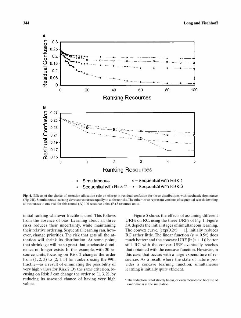
Figure 4 shows how RC declines with the invest-ment of ranking resources according to differentAARs, either for 100 resource units (Fig. 4A) or justthe first 5 units (Fig. 4B). These resources are in-vested either equally in all three risks simultaneouslyor exclusively in one risk. In this case, as more rank-ing resources are invested, the RC value decreases,both for the simultaneous strategy and for any of thethree sequential ranking strategies (i.e., looking atjust a single risk during this ranking period). How-ever, the extent to which the overlap among the SPDsdecreases depends on the strategy: With 4 or more re-source units, RC is most efficiently reduced with si-multaneous learning, and increasingly so. An intui-tive account of this pattern is that with anyreasonable level of resources, each risk receivesenough attention to make a dent in its uncertainty.However, when resources are limited (Fig. 4B), se-quential risk ranking can be more effective, espe-cially when targeted at the risk causing the greatestconfusion. In this case, that is Risk 2, which overlapsboth of the other risks. For this reason, when re-sources are very limited, concentrating them all onRisk 2 is more efficient than concentrating on Risks 1or 3 (or spreading them across the three risksequally). However, when more resources are avail-able, they are wasted if spent just on that risk. By trialand error, we found an approximate optimum (notshown): devoting half the resources to Risk 2 andequal parts of the remainder to Risks 1 and 3. It is5–10% more efficient than simultaneous learning for5–40 resource units, then indistinguishable.

With simultaneous search, the risks retain theirFig. 3. Subjective probability distributions with (A) no overlap;(B) stochastic dominance; and (C) no stochastic dominance.


initial ranking whatever fractile is used. This followsfrom the absence of bias: Learning about all threerisks reduces their uncertainty, while maintainingtheir relative ordering. Sequential learning can, how-ever, change priorities. The risk that gets all the at-tention will shrink its distribution. At some point,that shrinkage will be so great that stochastic domi-nance no longer exists. In this example, with 30 re-source units, focusing on Risk 2 changes the orderfrom (1, 2, 3) to (2, 1, 3) for rankers using the 99thfractile—as a result of eliminating the possibility ofvery high values for Risk 2. By the same criterion, fo-cusing on Risk 3 can change the order to (1, 3, 2), byreducing its assessed chance of having very highvalues.

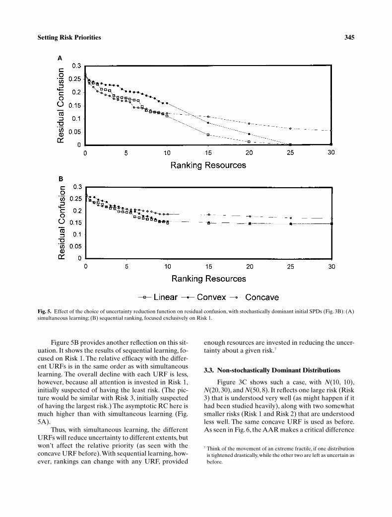
Figure 5 shows the effects of assuming differentURFs on RC, using the three URFs of Fig. 1. Figure5A depicts the initial stages of simultaneous learning.The convex curve, [exp(0.2

x

)

�

1], initially reducesRC rather little. The linear function (

y

�

0.5

x

) doesmuch better

6

and the concave URF [ln(

x

�

1)] betterstill. RC with the convex URF eventually reachesthat obtained with the concave function. However, inthis case, that occurs with a large expenditure of re-sources. As a result, where the state of nature pro-vides a concave learning function, simultaneouslearning is initially quite efficient.

6 The reduction is not strictly linear, or even monotonic, because ofrandomness in the simulation.

Fig. 4. Effects of the choice of attention allocation rule on charge in residual confusion for three distributions with stochastic dominance(Fig. 3B). Simultaneous learning devotes resources equally to al three risks. The other three represent versions of sequential search devotingall resources to one risk for this round: (A) 100 resource units; (B) 5 resource units.


Figure 5B provides another reflection on this sit-uation. It shows the results of sequential learning, fo-cused on Risk 1. The relative efficacy with the differ-ent URFs is in the same order as with simultaneouslearning. The overall decline with each URF is less,however, because all attention is invested in Risk 1,initially suspected of having the least risk. (The pic-ture would be similar with Risk 3, initially suspectedof having the largest risk.) The asymptotic RC here ismuch higher than with simultaneous learning (Fig.5A).

Thus, with simultaneous learning, the differentURFs will reduce uncertainty to different extents, butwon’t affect the relative priority (as seen with theconcave URF before). With sequential learning, how-ever, rankings can change with any URF, provided

enough resources are invested in reducing the uncer-tainty about a given risk.

7

3.3. Non-stochastically Dominant Distributions

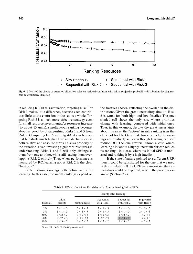
Figure 3C shows such a case, with

N

(10, 10),

N

(20, 30), and

N

(50, 8). It reflects one large risk (Risk3) that is understood very well (as might happen if ithad been studied heavily), along with two somewhatsmaller risks (Risk 1 and Risk 2) that are understoodless well. The same concave URF is used as before.As seen in Fig. 6, the AAR makes a critical difference

7 Think of the movement of an extreme fractile, if one distributionis tightened drastically, while the other two are left as uncertain asbefore.

Fig. 5. Effect of the choice of uncertainty reduction function on residual confusion, with stochastically dominant initial SPDs (Fig. 3B): (A)simultaneous learning; (B) sequential ranking, focused exclusively on Risk 1.


in reducing RC. In this simulation, targeting Risk 1 orRisk 3 makes little difference, because each contrib-utes little to the confusion in the set as a whole. Tar-geting Risk 2 is a much more effective strategy, evenfor small resource investments. As resources increase(to about 15 units), simultaneous ranking becomesabout as good, by distinguishing Risks 1 and 3 fromRisk 2. Comparing Fig. 6 with Fig. 4A, it can be seenthat RC starts much higher here and declines less, inboth relative and absolute terms. This is a property ofthe situation. Even investing significant resources inunderstanding Risks 1 and 3 will only distinguishthem from one another, while still leaving them over-lapping Risk 2 entirely. Thus, when performance ismeasured by RC, learning about Risk 2 is the clear“best buy.”

Table I shows rankings both before and afterlearning. In this case, the initial rankings depend on

the fractiles chosen, reflecting the overlap in the dis-tributions. Given the great uncertainty about it, Risk2 is worst for both high and low fractiles. The oneshaded cell shows the only case where prioritieschange with learning, compared with initial ones.Thus, in this example, despite the great uncertaintyabout the risks, the “action” in risk ranking is in thechoice of fractile. Once that choice is made, the rank-ings are relatively set, even though learning can stillreduce RC. The one reversal shows a case wherelearning a lot about a highly uncertain risk can reduceits ranking—in a case where its initial SPD is unbi-ased and ranking is by a high fractile.

If the state of nature pointed to a different URF,then it could be substituted for the one that we usedin this simulation. If the URF were uncertain, then al-ternatives could be explored, as with the previous ex-ample (Section 3.2).

Fig. 6. Effects of the choice of attention allocation rules on residual confusion with initial subjective probability distributions lacking sto-chastic dominance (Fig. 3C).

Table I.

Effect of AAR on Priorities with Nondominating Initial SPDs

Priority after learning

FractilesInitial

priority SimultaneousSequentialwith Risk 1

Sequentialwith Risk 2

Sequentialwith Risk 3

1% 2

�

1

�

3 2

� 1 � 3 2 � 1 � 3 2 � 1 � 3 2 � 1 � 35% 2 � 1 � 3 2 � 1 � 3 2 � 1 � 3 2 � 1 � 3 2 � 1 � 3

50% 1 � 2 � 3 1 � 2 � 3 1 � 2 � 3 1 � 2 � 3 1 � 2 � 390% 1 � 2 � 3 1 � 2 � 3 1 � 2 � 3 1 � 3 � 2 1 � 2 � 399% 1 � 3 � 2 1 � 3 � 2 1 � 3 � 2 1 � 3 � 2 1 � 3 � 2

Note: 100 units of ranking resources.


4. MODEL APPLICATION:BIASED INITIAL SPDS

4.1. Systematic Bias

Sometimes, initial beliefs are suspected of beingbiased. For example, it may seem as though research-funding priorities have unduly focused on studyingsome physical processes, or that publication pro-cesses have unduly favored results creating a particu-lar picture of risk. Those suspicions are, however, toodiffuse to be captured in the SPDs.8 This section con-siders one extreme type of suspicion: systematic bi-ases, which have the same direction and magnitudefor all risks. Such a condition might arise, say, whenpeople make the same mistake all the time (e.g., look-ing for trouble leads them to exaggerate all risks;their analyses share an erroneous parameter esti-mate). The next section briefly considers the other ex-treme, random biases.

As an example of systematic bias, we took theinitial SPDs of Fig. 3C, but altered the true SPDs (bybiasing the mean of the distribution upward by a fac-tor of two), while leaving the standard deviation thesame. In model terms, learning about a risk meanssampling observations from the true SPD, then com-bining those observations with the biased prior in aBayesian manner. That process will tend to reveal(and reduce) the bias. Depending on the circum-stances, the overall result might be to increase or de-crease uncertainty. Figure 7 shows the effect of learn-ing on estimates of the mean for Risk 1, as a functionof investing resources in Risk 1 alone or in all threerisks simultaneously. The same (concave) URF isused. The mean approaches the unbiased value (thelower dashed line) with either AAR, but does somore quickly when learning focuses on Risk 1 thanwhen it is distributed over all three risks. A similarpattern emerges with the other two risks, with fo-cused learning being moderately more efficient thansimultaneous. Thus, for this case, in which all risks arebiased in the same way, simultaneously learningseems advisable—in order to learn something abouteach risk—rather than to focus on any one. Of course,less progress would be made if the new informationwere also obtained from biased distributions (asmight happen if rankers relied on the same faultysources).

Figure 8 shows RC, investing the same resources

8 They might, however, be expressed in second-order distributions,expressing epistemic uncertainty(24)—a possibility that we will notconsider here.

in sequential or simultaneous learning. Simulta-neous learning shifts all distributions in the same di-rection. Given the common bias, that alone wouldleave RC relatively constant. However, a givenamount of resources will update a distribution withsmall initial variance more than a distribution withlarge initial variance. As a result, Risk 2 moves to-ward its mean more slowly than do Risk 1 and Risk 3.That increases its overlap with Risk 3, as well as theoverlap of Risk 1 and Risk 3—leading RC to increasewith such simultaneous learning. Risk 3’s initialmean is 50 and its true mean is 25, closer to Risk 2’sinitial mean. As a result, learning just about Risk 3will move its SPD toward that for Risk 2, increasingtheir overlap (and RC). As mentioned, Risk 2’s ini-tial SPD has a mean of 20, while its true SPD has amean of 10, the same as Risk 1’s initial mean. Thus,learning about just Risk 2 will shift the mean of itsSPD toward that of Risk 1, greatly increasing thecontribution to RC of that overlap, while shifting itsSPD away from Risk 3, somewhat decreasing thecontribution to RC of that overlap. At the same time,reducing Risk 2’s uncertainty will decrease its over-lap with the other two SPDs, somewhat reducing RC.The net effect is the small overall reduction in RCshown in Fig. 8 (Sequential with Risk 2). Reducingthe bias in Risk 1 still leaves it overlapping Risk 2;however, both the shift and the reduced uncertaintymake it more distinct from Risk 3, slightly reduc-ing RC.

Thus, learning about these risks does little toreduce rankers’ confusions and may increase it—because they were less confused initially than theyhad a right to be. Where bias is suspected, RC doesnot provide a criterion for evaluating the efficacy ofdifferent strategies.

If these risks are ranked by the means of theirSPDs, their initial order is (1, 2, 3). It remains thatway whatever AAR is used. Simultaneous learningshifts all three means in tandem. None of the sequen-tial learning rules pulls the focal mean past one of theothers; as a result, their order stays the same. Initialranking by the 95th fractile is (1, 3, 2) because of Risk2’s long right tail. The order will change to (1, 2, 3) ifenough is learned about Risk 2 to pull in its tail andshift the distribution to the left.

4.2. Random Bias

Systematic bias describes one extreme. Anotherextreme involves biases that are completely random,in both direction and magnitude (over some range of


possibilities). In this case, all the complications dis-cussed above could happen, with the results of thesimulations (and the ranking processes that they rep-resent) being even less predictable. As before (Sec-tion 4.1), learning about the risks may appropriatelyincrease uncertainty.

If bias is suspected, then it may pay to do someexploratory learning about the risks. If the width ofthe SPDs increases, then bias should be morestrongly suspected. If the SPD shifts are in a commondirection, then systematic bias is more likely. Themodel built for that situation could then incorporate

these assumptions when trying to design a rankingprocess or to predict its operation.

5. CONCLUSIONS ANDPOLICY IMPLICATIONS

Individuals, organizations, and societies oftenneed priorities for addressing the myriad risks totheir health, safety, and environment. Deciding onthose priorities should help them to focus their searchfor ways to reduce risk. When risks are uncertain, somay be these priorities. Learning about risks may al-

Fig. 8. Residual confusion with biased initial and an unbiased learning process, for simultaneous learning and sequential learning, focusedon each risk.

Fig. 7. Change in degree of bias, with simultaneous ranking and sequential ranking focused on learning about Risk 1.


low reducing residual uncertainty about both their in-dividual magnitudes and their respective rankings.

We offer a model for such processes. It assumesan iterative process, in which limited resources aredevoted to uncertainty reduction during successivelearning periods, and rankings are revised in the lightof what is learned. The model characterizes eachround in terms of two states of nature, which peoplecannot control, and four design parameters, whichthey can. The states of nature are (1) the uncertainty,expressed in SPDs (which might be biased) and (2)the pace with which uncertainty shrinks, when re-sources are invested in learning about a risk (ex-pressed in URFs). The design parameters are (1) theAAR, describing how learning resources are allo-cated across risks; (2) the ranking criterion, or fractileused to characterize the SPDs, for ranking purposes;(3) the Bayesian (or other) updating rule for combin-ing new information about a risk with existing infor-mation; and (4) the RC measure for evaluatingperformance (which, however, is not directly inter-pretable when initial SPDs are suspected of bias).

Demonstrations of the model focus on two of themany possible ways in which attention can be allo-cated (during a round): simultaneous learning, whereall risks receive equal attention, and sequential learn-ing, where all learning resources are allocated to asingle risk (for that round). The demonstrations con-sider the learning associated with three classes of theuncertainty reduction function: linear, concave, andconvex.

The impact of these factors was examined in thecontext of five different initial conditions. Three ofthese assumed no underlying bias in the initial SPDs:(1) virtually no overlap among the distributions, (2)stochastic dominance, and (3) no stochastic domi-nance. The third of these situations was reconsidered,assuming bias in the initial SPDs that was either sys-tematic or random.

In all cases, a Bayesian updating function wasused to integrate what is learned with what was ini-tially believed. For computational simplicity, we alsorestricted ourselves to one set of conjoint distribu-tions (normal). A straightforward way to relax theoptimality assumption is to use Bayesian updating,but over- or underweight the new information,thereby representing rankers who are too quick orslow to change.

Also for simplicity’s sake, demonstrations haveused only three risks. However, we hope that they il-lustrate the key features of the model and how it canilluminate the structure of risk-ranking tasks. In some

cases, just characterizing a ranking process in theseterms may clarify how efficient, and appropriate, it is.For example, it may reveal whether the critical uncer-tainties are about facts or values. It might forestalllarge-scale data collection when there is little agree-ment about the risk metric, the ranking criterion, orthe performance measure.

In other cases, though, it may be necessary actu-ally to run the numbers. For example, in the examplewith stochastic dominance (Section 3.2), we foundthat the choice of AAR influenced both the finalrankings and the efficiency of ranking strategies. Withfewer resources, devoting them all to one risk couldbe more efficient than dividing them equally acrossthe risks. With greater resources, however, simulta-neous learning would be more efficient than sequen-tial. In the example without stochastic dominance(Section 3.3) the choice of AAR greatly affected howfar RC was reduced. The same was true when therewas bias in the initial SPDs. Resources could bewasted if these issues were not sorted out before aranking exercise was designed—or its results were in-terpreted. Even in our simple examples, these rela-tionships would be hard to anticipate without explicitquantitative modeling.

We see value in characterizing stylized situationslike those considered here. Doing so provides a wayto think about the nature of risk ranking, includingwhat one hopes to—and realistically can—gain fromit. We also sought, however, to characterize themodel clearly enough to allow its operationalizationfor specific settings. We now sketch how each of themodel’s parameters might be approached in an appli-cation, either designing a process or predicting its ef-ficacy. These steps could be followed for the specificrisks under consideration or for a small set of riskswith properties like those in the full set (e.g., hetero-geneous variance, no systematic bias, many risks clus-tered near the bottom of the set). Such archetypesmight provide a useful feeling for the results of a full-fledged application.

States of NatureSPDs: Follow accepted procedures for pro-bability elicitation.(18,25) Elicit suspicions ofbias, perhaps in the form of second-orderdistributions.URF: Consider the state of the science re-garding each risk. How ripe is it for summari-zation?(26) What kinds of diagnostic tests areavailable (e.g., just rodent bioassays or alsobacterial tests)? How quickly can novices bebrought up to speed?


Design ChoicesRanking criterion: Elicit rankers’ preferencesfor the fractile best suited to characterizinguncertain risks.AAR: Start with a suite of stylized rules, in-cluding entirely systematic and sequentiallearning, along with promising hybrids.Translating these rules into URF terms maybe challenging, even if the general shape ofthe URF is fairly clear. Once the other termsof the model have been set, backing out thebest AARs is a logical way to optimize itsapplication.Performance measure: While simple, our RCmetric treats distributional overlap the same,at all points on the risk continuum. It meansthat all confusion is equally troubling. Rank-ers might, however, choose to pay more atten-tion to confusion among larger risks. Doing sowill require a risk metric with more than inter-val-scale properties.Updating: Although the designers of a rank-ing process might prescribe a Bayesian ap-proach, other expectations might be more re-alistic. In that case, updating is a state ofnature, knowledge of which will help in pre-dicting how a ranking process will actuallybehave.

Although the model is fairly complex already,we can see several elaborations that could improve itsfidelity, facilitate its application, and increase its de-sign flexibility. One is to include variability as asource of the uncertainty in an SPD. Because vari-ability is more directly estimated than uncertaintiesderived from other sources, considering it should re-fine the analysis. A second elaboration is to distin-guish uncertainty about facts and about values. Partof a ranking process is determining what mattersmost, when integrating multiple attributes into acommon measure of risk. Thinking hard about theranking of some risks may teach useful lessons aboutthe meaning of “risk” in general. Therefore, focusedlearning about a subset of risks might reduce confu-sion about the set as a whole. As a result, one hybridstrategy is to look closely at a few risks, in order to re-solve the definition of “risk,” then to think simulta-neously about all risks in those terms.

In such ways, a model like this one can take ad-vantage of experiences with risk ranking—and iden-tify aspects of those processes that need to be betterunderstood. Thus, one might look for structural prop-

erties of actual risk rankings that have been more orless satisfactory for participants. Are value issuesbrought to the fore, or left unarticulated beneath dis-cussions of data? Has the technical staff provided co-gent summaries of the issues, so that the rankers canlearn a lot quickly—even if it would take them a verylong time to acquire great mastery (making the URFmore concave)? Is increased uncertainty an accept-able conclusion, when biased priors (and prematureclosure) are possibilities? Have the rankers been re-quired to look at all the risks, when sequential evalu-ation of a few would have been more effective?

ACKNOWLEDGMENTS

The authors thank Mike DeKay, Paul Fischbeck,Keith Florig, Granger Morgan, Andy Parker, Mitch-ell Small, and two anonymous reviewers for theirvaluable comments on this work. This research wassupported by National Science Foundation GrantSBR-9512023 and Environmental Protection AgencyGrant CR824706-01-02; however, the views ex-pressed here are those of the authors alone.

REFERENCES

1. Davies, J. C. (Ed.). (1996). Comparing environmental risks.Washington, DC: Resources for the Future.

2. Morgan, M. G., Fischhoff, B., Lave, L., & Fischbeck, P. (1996).A proposal for ranking risk within federal agencies. In C.Davies (Ed.), Comparing environmental risks (pp. 111–147).Washington, DC: Resources for the Future.

3. U.S. Environmental Protection Agency. (1987). Unfinishedbusiness: A comparative assessment. Washington, DC: Author.

4. U.S. Environmental Protection Agency. (1991). Reducingrisks: Setting priorities and strategies for environmental protec-tion. Washington DC: Author.

5. Jones, K. (1997). Ten years of comparative risk analysis. http://www.greenmount.com (XX XXX XXX).

6. Minard, R. A., Jr. (1996). CRA and the states: History, politics,and results. In J. Clarence Davis (Ed.), Comparing environ-mental risks—tools for setting government priorities. Washing-ton, DC: Resources for the Future.

7. National Research Council. (1996). Understanding risk. Wash-ington, DC: Author.

8. Lindblom, C. (1959). The science of muddling through. PublicAdministration Review, 19, 79–88.

9. Bendor, J. (1995). A model of muddling through. AmericanPolitical Science Review, 89, 819–840.

10. Crouch, E.A.C., & Wilson, R. (1981). Risk/benefit analysis.Cambridge, MA: Ballinger.

11. Fischhoff, B., Watson, S., & Hope, C. (1984). Defining risk.Policy Sciences, 17, 123–139.

12. Fischhoff, B., Slovic, P., Lichtenstein, S., Read, S., & Combs, B.(1978). How safe is safe enough? A psychometric study of at-titudes towards technological risks and benefits. Policy Sci-ences, 8, 127–152.

13. Jenni, K. (1997). Attributes for risk evaluation. Unpublished

Q3

Q4a

Q2


doctoral dissertation, Carnegie Mellon University, Pittsburgh,PA.

14. Slovic, P., Fischhoff, B., & Lichtenstein, S. (1979). Rating therisks. Environment, 21(4), 14–20, 36–39.

15. Slovic, P., Fischhoff, B., & Lichtenstein, S. (1980). Facts andfears: Understanding perceived risk. In R. Schwing & W. A.Albers, Jr. (Eds.), Societal risk assessment: How safe is safeenough? (pp. 181–214).

16. Kahneman, D., Slovic, P., & Tversky, A. (Eds.). (1982). Judg-ments under uncertainty: Heuristics and biases. New York:Cambridge University Press.

17. Kammen, D., & Hassenzahl, D. (1999). Should we risk it?Princeton, NJ: Princeton University Press.

18. Morgan, M. G., & Henrion, M. (1991). Uncertainty. New York:Cambridge University Press.

19. Kingdon, J. W. (1995). Agendas, alternative and public policies.Little, Brown and Company.

20. Slovic, P., Fischhoff, B., & Lichtenstein, S. (1985). Characteriz-ing perceived risk. In R. W. Kates, C. Hohenemser, & J.

Kasperson (Eds.), Perilous progress: Managing the hazards oftechnology (pp. 91–125). Boulder, CO: Westview.

21. Edwards, W., Lindman, H., & Savage, L. S. (1963). Bayesianstatistical inference for psychological research. PsychologicalReview, 70, 193–242.

22. Fischhoff, B., & Beyth-Marom, R. (1983). Hypothesis evalua-tion from a Bayesian perspective. Psychological Review, 90,239–260.

23. Slovic, P., & Lichtenstein, S. (1971). Comparison of Bayesianand regression approaches to the study of information pro-cessing in judgment. Organizational Behavior & Human Per-formance, 6, 649–744.

24. Gärdenfors, P., & Sahlin, N. E. (1982). Unreliable probabili-ties, risk taking and decision making. Synthese, 53, 361–386.

25. Clemen, R. (1991). Making hard decisions: An introduction todecision analysis. Boston: PWS-Kent.

26. Funtowicz, S., & Ravetz, J. (1990). Uncertainty and quality inscience for policy. London: Kluwer.

Q7

Q8

Q4b

Q5

Q6

Risk Analysis 20(3) JuneQuery Sheet

Author: Please print this file, and respond to the following queries. Insert additions/corrections inthe exact location on the page where changes need to be made; and return the completeset of proofs to the address given on the cover sheet.

Q1: Please clarify and provide complete mailing address.

Q2: “backing” OK?

Q2a: Please cite Ref. 9 in text.

Q3: Please provide closing sentence, rather than ending article with a question.

Q4a: Please provide date last accessed—a required element of online citations.

Q4b: Change to “unpublished” OK? Also, Pittsburgh location OK for Carnegie Mellon

University?

Q5: Please provide publisher name and location

Q6: Please provide place of publication

Q7: OK? Gärdenfors & Sahlin authors, not editors?

Q8: Unfamiliar with PWS-Kent—correct and complete publisher name?

Documents

Setting Risk Priorities: A Formal Model - Social and …sds.hss.cmu.edu/risk/articles/Risk032.pdfSetting Risk Priorities 341 has at least interval-scale properties. As mentioned, the