NBER WORKING PAPER SERIES

SET-ASIDES AND SUBSIDIES IN AUCTIONS

Susan AtheyDominic CoeyJonathan Levin

Working Paper 16851http://www.nber.org/papers/w16851

NATIONAL BUREAU OF ECONOMIC RESEARCH1050 Massachusetts Avenue

Cambridge, MA 02138March 2011

We thank Enrique Seira for his collaboration in assembling the data for this paper, Matt Osborne andFrank Zhuo for research assistance, and Ken Hendricks for comments on an early draft of this paper.The National Science Foundation provided generous financial support. The views expressed hereinare those of the authors and do not necessarily reflect the views of the National Bureau of EconomicResearch.

NBER working papers are circulated for discussion and comment purposes. They have not been peer-reviewed or been subject to the review by the NBER Board of Directors that accompanies officialNBER publications.

© 2011 by Susan Athey, Dominic Coey, and Jonathan Levin. All rights reserved. Short sections oftext, not to exceed two paragraphs, may be quoted without explicit permission provided that full credit,including © notice, is given to the source.

Set-Asides and Subsidies in AuctionsSusan Athey, Dominic Coey, and Jonathan LevinNBER Working Paper No. 16851March 2011JEL No. D44,H57,L53

ABSTRACT

Set-asides and subsidies are used extensively in government procurement and natural resource sales.We analyze these policies in an empirical model of U.S. Forest Service timber auctions. The modelfits the data well both within the sample of unrestricted sales where we estimate the model, and whenwe predict (out of sample) bidder entry and prices for small business set-asides. Our estimates suggestthat restricting entry to small businesses substantially reduces efficiency and revenue, although it doesincrease small business participation. An alternative policy of subsidizing small bidders would increaserevenue and small bidder profit, while eliminating almost all of the efficiency loss of set-asides, andonly slightly decreasing the profit of larger firms. We explain these findings by connecting to the theoryof optimal auction design.

Susan AtheyHarvard UniversityDepartment of Economics1875 Cambridge St.Cambridge, MA 02138and NBERathey@fas.harvard.edu

Dominic CoeyStanford UniversityDepartment of Economics579 Serra MallStanford CA 94305-6072dcoey@stanford.edu

Jonathan LevinStanford UniversityDepartment of Economics579 Serra MallStanford, CA 94305-6072and NBERjdlevin@stanford.edu

An online appendix is available at:http://www.nber.org/data-appendix/w16851

1. Introduction

Government procurement programs often seek to achieve distributional goals in addition

to other objectives. In the United States, the federal government explicitly aims to award at

least 23% of its roughly $400 billion in annual contracts to small businesses, with lower targets

for businesses owned by women, disabled veterans and the economically disadvantaged.1

Many state and local governments also set goals regarding small businesses or locally owned

�rms. Given the large scope of these programs, it is perhaps surprising that relatively little

is known about the optimal design of preference programs and their costs.

Two common methods are employed to achieve distributional goals. One approach is

to set aside a fraction of contracts for targeted �rms. For instance, federal procurement

contracts between $25,000 and $100,000 are typically reserved for small businesses.2 An

alternative is to provide bid subsidies for favored �rms. Subsidies are used by the Fed-

eral government to assist domestic �rms bidding for construction contracts under the Buy

America Act, by the Federal Communications Commission to favor minority-owned �rms in

spectrum auctions, and in California state highway procurement to assist small businesses.

This paper develops and estimates an econometric model of entry and bidding in auctions,

and uses it to simulate the revenue and e¢ ciency consequences of using alternative market

designs to achieve distributional objectives. Our empirical setting is the U.S. Forest Service

timber sale program, which conducts both set-aside sales and unrestricted sales, but does

not use subsidies. During the time period we study, the Forest Service sold around a billion

dollars of timber a year, and in the region from which our data is drawn, 14% of the sales are

small business set-asides. We �nd that designating a sale as a set-aside reduced e¢ ciency by

17% and cost the Forest Service about 5% in revenue. Providing a subsidy to small bidders

in all auctions appears to be a more e¤ective means of achieving distributional goals. A

range of subsidies might have eliminated both e¢ ciency and revenue losses, while allocating

the same volume of timber to small bidders, increasing aggregate small �rm pro�ts, and

1Section 15(g)(1) of the Small Business Act reads: �The Government wide goal for participation by smallbusiness concerns shall be established at not less than 23 percent of the total value of all prime contractawards for each �scal year.�Extensive documentation of US government procurement programs for smallbusinesses can be found on the Small Business Administration website at http://www.sba.gov/.

2See 15 USC 644(g)(1) or the Federal Acquisitions Regulations, Section 19.502-2.

1

only slightly reducing the pro�t of larger �rms. If other U.S. procurement and resource

allocation programs are similar, these results suggest that billions of dollars might be at

stake in undertaking a redesign of set-asides.

Basic supply and demand suggests that set-aside programs should lower revenue and

decrease e¢ ciency by reducing the number of eligible buyers. This need not be the case,

however, if bidding is costly and �rms are heterogeneous. In such a setting, restricting par-

ticipation may increase auction revenue. Suppose there is a single large bidder with a value

uniformly distributed between 0 and 30 and two small �rms with values uniformly distributed

between 0 and 10. If it costs seventy-�ve cents to learn one�s value and enter the auction, the

large bidder will be the only entrant and will win at a zero price. If participation is restricted

to the small �rms, both will enter and the expected price increases from 0 to 313, despite

the fact that expected social surplus decreases by 9 112. If there are more large �rms to begin

with, however, or if entry costs are substantially lower or higher, a set-aside program both

lowers revenue and decreases e¢ ciency.3 Thus, both entry and bidding behavior must be

considered in a full analysis of these programs.

Bid subsidies also can have ambiguous e¤ects depending on the relative strengths of

the bidders and the costs of participation. A well-known insight of Myerson (1981) is that

appropriately handicapping bidders can increase revenue relative to a standard open or sealed

bid auction. The impact of a �xed subsidy, however, can depend subtly on bidders�value

distributions, as discussed by McAfee and McMillan (1989). Moreover, with endogenous

participation, a subsidy will a¤ect entry in ways that in principle can be helpful or harmful.

In the previous example, a rule that awards the object to a small bidder if its bid is at

least a third that of the large bidder generates entry by all three �rms. Expected revenue

increases from zero to 813with social surplus decreasing by 4. Such a program results in a

small �rm winning two-thirds of the time. Less dramatic subsidies have a similar qualitative

e¤ect, raising revenue while decreasing surplus. A larger subsidy, however, may discourage

participation by the large �rm; for some entry costs, the result can be lower revenue than a

3Suppose, for instance, there are two large �rms. Then absent an entry restriction, both large �rms enter inequilibrium, giving an expected price of 10. And a participation restriction decreases both revenue and socialsurplus. The e¤ects of restricting participation also can depend on features other than costly participation,e.g. Bulow and Klemperer (2001) show that restricting participation sometimes can be bene�cial if thereare strong �winner�s curse�e¤ects.

2

no-subsidy sale.

Getting a handle on the e¤ect of set-asides or subsidies in a given setting requires under-

standing the relative strengths of targeted and non-targeted bidders. Forest Service timber

sales are characterized by a high degree of diversity in participating bidders. Bidders range

from small logging out�ts to large vertically integrated forest products companies. We dis-

tinguish between the smaller �rms that are eligible for set aside sales and the larger �rms

that are not. The smaller �rms are mainly logging companies, while the large �rms are mills

and often part of larger forest product companies. The relative strength of these bidders

varies with the size of the sale. For the smallest quintile of sales by volume, the di¤erent

types of bidders do not submit signi�cantly di¤erent bids. In larger sales, the small �rms

bid substantially less, and our estimates imply an even greater di¤erence in underlying valu-

ations. One explanation for the bidding and value di¤erences is that large mills can process

large quantities of timber more e¢ ciently or avoid frictions in re-selling harvested logs.

We next develop a model of bidder entry and bidding and estimate its parameters from

the data. Building on Athey, Levin and Seira (2011, hereafter ALS), we model each sale

as a private value auction with endogenous entry. As we wish to use the model to assess

counterfactual changes in the preference policy (i.e. varying entry restrictions and subsidy

levels), it is important to have an econometric model that can accurately predict entry and

prices �out-of-sample� as preference policies change. Thus, we estimate the model using

only data from unrestricted sealed bid sales, and assess its performance by comparing the

out-of-sample predictions for small business set-asides with the actual outcomes in the data.

The model performs well: predicted prices and entry are within 5% of observed values, and

we cannot reject equality of the predicted and observed bid distributions.

One observation from comparing unrestricted and set-aside sales is that entry responses

help to mitigate the losses from set-aside policies. If small bidders did not increase their

participation relative to unrestricted sales, revenue and e¢ ciency losses both would be larger

(30 and 28 percent, respectively, rather than 5 and 17 percent).

We also use the model to calculate the e¤ect of implementing a bidder subsidy program

(applied to all sales) in lieu of direct set-asides for a subset of sales.4 A range of subsidies

4The idea that the Forest Service set-aside program could be replaced with a subsidy policy is discussed

3

seem more e¤ective at achieving distributional goals than the observed policy of set-asides.

From a programmatic perspective, a 6% subsidy for small businesses would result in small

�rms winning as much timber as under the set-aside program, with 4% higher prices and a

2% increase in overall program e¢ ciency. There is a small decline in the expected pro�t of

larger �rm (less than 2%), which disappears entirely with a slightly smaller subsidy. The

attractive performance of subsidies relative to set-asides can be understood by connecting

our empirical model to the theory of optimal auction design, which we do in the �nal section

of the paper.

Another way to limit e¢ ciency losses while achieving distributional objectives is to select

sales to be set-asides where e¢ ciency losses would be small. We construct a statistical model

that selects sales into the set-aside program in a way that minimizes expected e¢ ciency losses

subject to a constraint of volume sold, and �nd that using this model to allocate sales into

the set-aside program would result in revenue and e¢ ciency that are virtually identical

to the no-preference policy. We also investigate the idea that a set-aside program serves to

�guarantee�a minimal level of timber for targeted �rms, reducing the risk that small bidders

will win little timber. However, we �nd that this bene�t is modest due to the relatively large

number of sales.

Our results can be usefully compared to recent �ndings of Marion (2007) and Kras-

nokutskaya and Seim (2010), who study the e¤ect of bid subsidies in California highway

procurement auctions.5 Marion compares state-funded auctions that have a small businesses

subsidy to federally-funded auctions with no subsidy. He �nds that procurement costs are

3.8% higher in the subsidy auctions, and attributes the increase to decreased participation by

large �rms in subsidy auctions. Krasnokutskaya and Seim use data from the subsidy auctions

to estimate a structural bidding model, and use the model to simulate alternative preference

policies. They conclude that the subsidy program has a very small e¤ect on procurement

costs, less than 1%.

by Froeb and McAfee (1988), and also by Brannman and Froeb (2000).5Several other papers also simulate various types of preference policies as applications of estimated auc-

tion models. Examples include Brannman and Froeb (2000), Flambard and Perrigne (2008), Roberts andSweeting (2010). Brannman and Froeb�s paper, which looks at Forest Service timber auctions, is particularlyinteresting because although the approach is quite di¤erent from ours (they do not consider bidder partic-ipation, use di¤erent data, and consider a logit value model of second price auctions), they reach a similarconclusion about the revenue e¤ect of the Forest Service set-aside program.

4

An intermediate �nding in these papers, and one that contrasts with our setting, is

that the large �rms in the California highway auctions do not appear to have much of a

cost advantage, so the �Myerson e¤ect�of subsidies is small. Another di¤erence is that we

estimate a complete model of entry and bidding using data on non-set-aside auctions, and

establish that our model provides accurate predictions (out of sample) of the outcomes in

small business set aside sales, providing greater con�dence in our counterfactual simulations.6

That being said, all three studies share a central theme, which is that accurately accounting

for participation is crucial in assessing bid preference programs.

2. A Model of Set-Asides and Subsidies

This section describes our basic model of the auction process, which builds on ALS. We

then use the model to informally discuss the e¤ect of set-asides or bidder subsidy programs.

A. The Model

Consider a seller who wishes to auction a single tract of timber. She announces a re-

serve price r, and whether the auction will be open or sealed bid. There are NS potential

small bidders and NB potential big bidders. The potential bidders have values that are in-

dependently distributed according to either FS or FB depending on the bidder�s size. These

distributions have densities f� and supports [0; v� ] for � = S;B. A bidder must spend K

to learn its private value and enter the auction. After the entry decisions are made, each

participant learns the identities of the other participants before bids are submitted. In a

sealed bid auction, the highest bidder wins and pays its bid. In an open auction, the highest

bidder wins and pays the second highest bid (or the reserve price if there is a single bidder).

The analysis of the bidding game is standard. With sealed bidding, there is a unique

Bayesian Nash equilibrium in which the bidders bid their values minus a shading factor

that depends on the equilibrium behavior of opponents. We state and use the �rst order

conditions for equilibrium in Section 4. With an open auction, there is an equilibrium in

6There are also a number of speci�c modeling di¤erences, for instance in the way the papers model entrybehavior (mixed strategies versus pure strategies with incomplete information about entry costs), whatbidders know about their competitiors when they submit their bids, and in the parametric modeling of biddistributions.

5

weakly dominant strategies in which each bidder continues in the auction until the price

reaches its valuation, at which point it drops out.

In the entry game, we focus on type-symmetric equilibria. Small and big bidders enter

with probabilities denoted (pS; pB), and entrants earn an expected pro�t of at least K. In

set-asides, pB = 0. Later, we distinguish three types of non-set-aside sales, based on our

observation that large �rms appear to have higher values than small �rms in most sales,

but not the very smallest sales. In typical sales, where we estimate that large �rms have

substantially higher values, we focus on equilibria in which big bidders enter the auction

(pB = 1), and small bidders randomize their entry with equal probability.7 In small sales

without subsidies, FS = FB and we focus on the unique fully symmetric equilibrium in

which pS = pB. In small sales with a subsidy for small bidders, we consider the full set of

type-symmetric equilibria.

We should emphasize that modeling entry requires a number of choices that can be

debated. For instance, our focus on type-symmetric entry equilibria involves looking at

mixed strategies. While symmetry is a standard restriction, mixed strategy equilibria have

the somewhat unintuitive property that decreasing the number of potential bidders � for

example, due to a set-aside program � potentially can increase expected participation and

revenue.8 This �coordination e¤ect�originally motivated us to focus on pure strategy entry

equilibria. But as we discuss in Section 4, that approach led us to estimate implausibly high

entry costs for many low entry sales. Subsequently we found that our estimates with mixed

strategy entry do not imply signi�cant coordination e¤ects, alleviating our initial concern.

In addition to deciding whether to focus on pure or mixed equilibria, or symmetric equi-

libria, or all possible equilibria, one can ask if bidders have private information about their

values prior to making entry decisions, whether they have or acquire common information

that is unobserved to the econometrician, and whether they can acquire information about

7With a su¢ ciently large number of big bidders, another possibility would be that big bidders randomizeentry and small bidders for sure do not enter. As discussed in more detail in ALS, this does not appear tobe the empirically relevant case in our setting.

8This can happen even if all bidders are symmetric. Consider an auction with three potential bidders whohave values distributed uniformly on [0,10] and an entry cost of 10=3: With no entry restriction, all bidderswill enter with probability 2=3 in equilibrium and expected revenue will be 80=27. If one potential bidderis restricted from entering, the two remaining �rms will enter with probability 1 and expected revenue willincrease 10=3:

6

the level of likely competition. Recent papers that take di¤erent approaches to these issues

include Li (2005), Li and Zheng (2009), Bajari, Hong and Ryan (2009), Krasnokutskaya and

Seim (2010), Marmer, Shneyerov and Xu (2010) and Roberts and Sweeting (2010). The last

two papers allow bidders to have a degree of private value information before making their

entry decisions, and use variation in potential entry to aid identi�cation.9 On the other

hand, they make some assumptions that are not ideal for our purposes: Marmer, Shneyerov

and Xu (2010) assume that all bidders are symmetric and rule out unobserved heterogeneity

across auctions, while Roberts and Sweeting�s (2010) approach, at least in its current version,

is applicable only to open auctions.

B. Set-Aside Auctions

A small business set-aside excludes big bidders from the auction, but increases the in-

centives for small bidders to participate because they anticipate less competition. If the

small and big bidders have identical value distributions, and there are a su¢ cient number of

potential small entrants to substitute one for one for big entrants, a set-aside provision will

have no e¤ect on total participation, revenue or overall e¢ ciency. If there are not enough

potential small entrants to promote fully compensating entry, a set-aside will reduce total

entry, reduce revenue, and reduce e¢ ciency.

The e¤ects of a set-aside are less clear if the value distributions are asymmetric. The

reason is that, as explained in the introduction, the increase in small bidder participation

can lead to a greater overall number of auction entrants, and potentially, to higher expected

revenue. The e¤ect of a set-aside, both in direction and size, therefore depends on the number

and relative strength of potential bidders, the cost of entry, and the auction format. For the

open auction case, it is possible to show that a set-aside cannot increase total surplus because

the unrestricted entry equilibrium is socially e¢ cient � that is, it maximizes expected surplus

given the set of potential entrants and simultaneous entry decisions.

C. Bidder Subsidies

A subsidy program favors the bids of certain �rms. A typical approach is to say that a

9This requires a good estimate of potential entry, which is not the strongest aspect of our data. On theother hand, our data has excellent information on realized entry, even for open auctions, which is somethingthat our approach exploits.

7

favored bidder must pay only a portion b= (1 + �) of its bid b for some � > 0. (One can also

make the bid credit an absolute amount rather than a fraction of the bid.) To illustrate the

e¤ects of a subsidy, suppose we have an open auction with two participants, a big bidder

with value vB and a small bidder with value vS. If the seller o¤ers a subsidy of size � to the

small bidder, there are three possible outcomes. If vS > vB, the subsidy will not change the

outcome of the sale, but it will lower revenue from vB to vB= (1 + �). If (1 + �) vS > vB > vS,

the subsidy will allow the small bidder to win over the higher-valued big bidder and revenue

will fall from vS to vB= (1 + �). Finally, if vB > (1 + �) vS, the big bidder will win with or

without the subsidy, but the policy will raise revenue by �vS.

From an ex-ante standpoint, it is relatively easy to see that if big bidders are stronger

a small subsidy will tend to increase sale revenue. A small subsidy is unlikely to a¤ect the

allocation and conditional on the allocation being una¤ected the big bidder is the likely

winner, so revenue increases. A similar logic applies even if there are more bidders, although

the subsidy can end up being irrelevant or neutralized if the high bidders are both small or

both big. A small subsidy will also increase small bidder participation without a¤ecting the

participation of large bidders, which leads to another positive revenue e¤ect, although at the

cost of distorting social e¢ ciency.

The situation becomes ambiguous if one considers larger subsidies. For �xed participation

the allocative distortions become larger, and strong but unfavored bidders also may be

deterred from participating. So in principle, some subsidies may reduce both revenue and

social e¢ ciency.

3. Description of Timber Sales

This section describes how timber auctions worked in the time period we consider, the

small business set-aside program, and the data for our study. We discuss only the essentials

of the sale process; more detailed accounts can be found in Baldwin, Marshall and Richard

(1997), Haile (2001), Athey and Levin (2001) or ALS.

A. Timber Sales and Small Business Set-Asides

8

A sale begins with the Forest Service identifying a tract of timber to be sold and con-

ducting a survey to estimate the quantity and value of the timber and the likely costs of

harvesting. A sale announcement that includes these estimates is made at least thirty days

prior to the auction. The bidders then have the opportunity to conduct their own surveys

and prepare bids. The Forest Service uses both open and sealed bid auctions. If the auction

is open, bidders �rst submit qualifying bids, typically at the reserve price, followed by an as-

cending auction. The sealed bid auctions are �rst price auctions. In either case, the auction

winner has a set period of time, typically between one and four years, to harvest the timber.

The Forest Service designates certain sales as small business set-asides. For a standard

set-aside sale, eligible �rms must meet two basic criteria. First, they must have no more

than 500 employees. Second, they must manufacture the timber themselves or re-sell it to

another small business, with the exception of a speci�ed fraction of the timber for which no

restrictions apply. In our data, there appear to be some exceptions to the eligibility criteria,

and conversations with Forest Service employees con�rm that the rules are occasionally

loosened for various reasons.

The Forest Service regulations also provide guidelines for which sales should be designated

as set-asides.10 The Forest Service periodically sets targets for the amount of timber small

businesses are expected to purchase in di¤erent areas. Though subject to some adjustment,

the basic goal is to maintain the historical share of timber volume logged by small businesses

in di¤erent areas, with the historical amounts corresponding to the quantities logged between

1966 and 1970. By projecting the amount of timber that will be purchased by small businesses

in unrestricted sales, the Forest Service determines the quantity of timber that must be sold

using set-aside sales, although forest managers have some discretion to accommodate speci�c

local needs. Forest managers are expected to use the same sale methods for set-aside sales

and to include a variety of sale sizes, terms and qualities in the set-aside program. Forest

managers do have some discretion to designate tracts as set-asides based on the needs of

small businesses in the area, which raises the possibility that tracts designated as set-asides

may be relatively well-suited to small �rms. We revisit this below.

B. Data and Descriptive Analysis10See the U.S. Forest Service Handbook, Section 2409.18 on Timber Sale Preparation.

9

Our data consists of sales held in California between 1982 and 1989. For each sale, we

know the identity and bid of each participating bidder, as well as detailed sale characteristics

from the sale announcement. We also collected additional information to capture market

conditions. We use national housing starts in the six months prior to a sale to proxy for

demand conditions, and U.S. Census counts of the number of logging companies and sawmills

in the county of each sale as a measure of local industry activity. Finally, for each sale, we

construct a measure of active bidders in the area by counting the number of distinct �rms

that bid in the same forest district over the prior year.

We use participation in set-aside sales, combined with internet searches on individual

�rms, to construct an indicator of small business status for each �rm. ALS distinguish

between mills that have manufacturing capability and logging companies that do not. Es-

sentially all of the logging companies are small businesses. The largest and most active mills

are not, but there are also some smaller mills that are eligible for set-asides.11 In this paper,

we classify bidders based on their small-business status (and refer to them as small and big)

rather than their manufacturing capability. An alternative would have been to treat small

mills as a separate category, but in later simulations that require us to compute sealed bid

auction equilibria, the inclusion of a third type of bidder adds complication to the already

challenging problem of accurate computation. We provide some additional discussion of the

small business classi�cation in Appendix A.

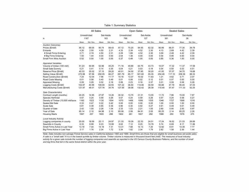
Table 1 presents summary statistics of tract characteristics and auction outcomes for

unrestricted and set-aside sales. The participation variables suggest that although set-asides

decrease the number of eligible bidders, this does not translate directly into a fall in realized

total participation. Additional participation by logging companies substitutes for the absent

mills. The table also shows that for both big and small tracts, prices are somewhat lower

when participation is restricted, although the di¤erence is not statistically signi�cant.

Data from unrestricted sealed sales suggests that the bidding behavior of big and small

bidders is on average quite di¤erent. To examine this more closely, we �rst stratify sales by

the volume of timber being auctioned. We then regress the logarithm of per-unit sealed bids

11We observe a few set-aside sales in which large mills entered, presumably because of exceptions made tothe rules. There are nine of these sales and we drop them from the analysis.

10

on auction �xed e¤ects and an indicator variable for big �rms. We do this separately for

sealed bid auctions in each sale size quintile. Table 2 shows the results. For the smallest

sales, the estimated di¤erence between the bids of small and large �rms is not statistically or

economically signi�cant, while big �rms bid about 11% more in second quintile tracts. The

coe¢ cients for larger tracts are imprecisely estimated because these sales are predominantly

open auctions, but the �nal column of the table shows that if we consider both the open

and sealed sales, larger sales are more likely to be won by big bidders. In our empirical

model below, we therefore allow the asymmetry between big and small bidders to depend

on the size of the sale, with no asymmetry for sales in the smallest quintile by volume, and

asymmetry for larger sales.

A key issue for our empirical analysis is the extent to which the tracts designated as set-

asides di¤er from those where participation is unrestricted. The tracts should be comparable

within a given forest based on Forest Service regulations, but forest managers also have some

discretion. Table 1 also indicates that at least on observable characteristics there are not

large di¤erences. To explore the point further, we use a logistic regression to estimate the

probability that a sale is set aside as a function of observable tract characteristics. The

results appear in Table 3. The most economically and statistically signi�cant explanatory

variables are the forest dummies, indicating that the use of set-asides varies across forest,

consistent with the USFS policy to preserve historical volumes allocated to small bidders.

Sales with higher logging costs (perhaps requiring more complex equipment) are less likely

to be small business set-asides. We control for the these tract characteristics in our empirical

models.

We then consider whether forest managers might designate as set-asides tracts that are

relatively more attractive to small bidders. We use the logit estimates to compute the esti-

mated probability that each tract is designated a set-aside; we refer to this as the �set-aside

propensity score.�We then consider the tracts that were not designated as set-asides and

estimate a logit regression to estimate the probability that the sale is won by a small bidder,

including the set-aside propensity score along with other sale characteristics as an explana-

tory variable. The propensity score is not signi�cantly related to the type of bidder that

wins the auction in either an economic or statistically signi�cant way (Appendix Table A3),

11

providing some evidence that set-asides are not designated on the basis of their attractiveness

to small bidders.

As a �rst pass at assessing the e¤ect of set-asides, we consider the linear model:

Y = � � SBA+X� + SBA �X + ": (1)

Here Y is an outcome of interest (total participation or log(revenue)), SBA is a dummy equal

to one if the sale is a small-business set-aside, and X is a vector of observed sale and forest

characteristics, including the propensity score from the logit regression described above. We

expect the set-aside e¤ect to vary across auctions, particularly as a function of sale size,

so we allow for alternative interaction e¤ects in our speci�cations. The key assumption for

identi�cation is that the choice of whether to make the sale a set-aside is uncorrelated with

unobservables that might directly a¤ect the outcome, that is " and SBA are independent

conditional on X.

We report regression results in Table 4. The reported estimates represent the average

e¤ect of set-aside status both over all tracts in the sample, and over those tracts that were

actually sold as set-asides (this is �̂ +X ̂, where X is the vector of the mean covariates of

the sales in question). The estimates suggest that set-asides reduce revenue and entry on an

average tract, and may increase entry on an average set-aside tract. The standard errors are

relatively large, re�ecting the modest sample size.

The structural model we estimate below allows us to go beyond these preliminary re-

gressions in two ways. First, we incorporate information on losing bids into the estimation,

which narrows the uncertainty in the estimated e¤ects. Second, it gives us a framework

for identifying the channels through which restricting entry a¤ects outcomes, as well as for

analyzing welfare and for evaluating a range of counterfactual subsidy policies.

4. Estimating Economic Primitives

We now calibrate our theoretical model from Section 2 and use it to analyze the impact

of di¤erent policies. The primitives of the model are the value distributions of the big

and small bidders, the entry cost for each auction, and the numbers of potential entrants.

12

We �rst estimate the value distributions, as a function of sale characteristics, from the

bid distributions in unrestricted sealed auctions. From these value distributions, we obtain

bidder pro�ts conditional on entry. We then estimate equilibrium entry probabilities for each

auction if entry of large bidders were unrestricted, as a function of sale characteristics and

entry patterns in the local geographic area. These entry probabilities, together with pro�ts

and our measure of potential entry, allow us to infer entry costs. In Section 5, we use the

estimated model to investigate the e¤ect of the set-aside program and to study the potential

impact of bidder subsidies.

A. Bidders�Value Distributions

Our approach to estimating the bidders�value distributions follows Guerre, Perrigne and

Vuong (2000), Krasnokutskaya (2011) and ALS. The �rst step �ts a parametric model of

the bid distributions in sealed auctions, allowing these distributions to depend on observed

sale characteristics and on an unobserved sale characteristic that accounts for within-auction

correlation of bids.12 The second step uses nonparametric methods to estimate the implied

value distributions. Estimates of these primitives allow us to compute expected bidder pro�ts

conditional on entry, and consequently to infer entry costs.

Let F� (�jX; u) denote the value distribution for a bidder of size � 2 fS;Bg conditional

on the observed sale characteristics X, and an unobserved sale characteristic u. We assume

that (X; u) and the number of actual participants n = (nS; nB) are common knowledge to

the bidders at the time they submit their bids. Consistent with our theoretical model, we

assume that bidder values are independent conditional on (X; u) and that participants use

equilibrium bidding strategies. If there is a single entrant to the auction, we assume he

bids the reserve price. With multiple entrants, we write the equilibrium bid distributions as

G� (�jX; u; n):

Based on our earlier observation that bidder heterogeneity appears to matter for most

12Krasnokutskaya was the �rst to point out the importance of allowing for unobserved auction hetero-geneity in estimating auction models, and how the Guerre et al. approach for sealed bid auctions couldbe extended in this direction. In principle, the open auction data also contain relevant information aboutbidder values, but the open outcry nature of these auctions is a complicating factor. See ALS for a discus-sion that summarizes points made by Athey and Haile (2002) and Haile and Tamer (2003). Roberts andSweeting (2010) use open auction data to estimate a model with unobserved heterogeneity by making use ofparametric assumptions.

13

sales, but not for the very smallest sales, we split the sample by sale size to estimate the

equilibrium bid distributions. That is, we distinguish the small tracts with timber volumes

in the lowest quintile from the larger tracts.

In each case, we follow ALS and assume that the unobserved auction characteristic u is

drawn from a Gamma distribution with mean one and variance �, independent of X and

n. We assume that conditional on (X; u; n), the bids of small and big �rms have a Weibull

distribution.13 That is, for � = S;B;

G� (bjX; u; n) = 1� exp �u �

�b

�� (X;n)

�p� (n)!: (2)

In equation (2), �� (�) is the scale is the scale of the Weibull distribution, parameterized as

ln�� (X;N; n) = X�X + n�n;� + �0;� , while �� (�) is the shape, parametrized as ln �� (n) =

n n;k + 0;k. For small sales, the bid distributions of the small and big �rms are modelled

as symmetric.

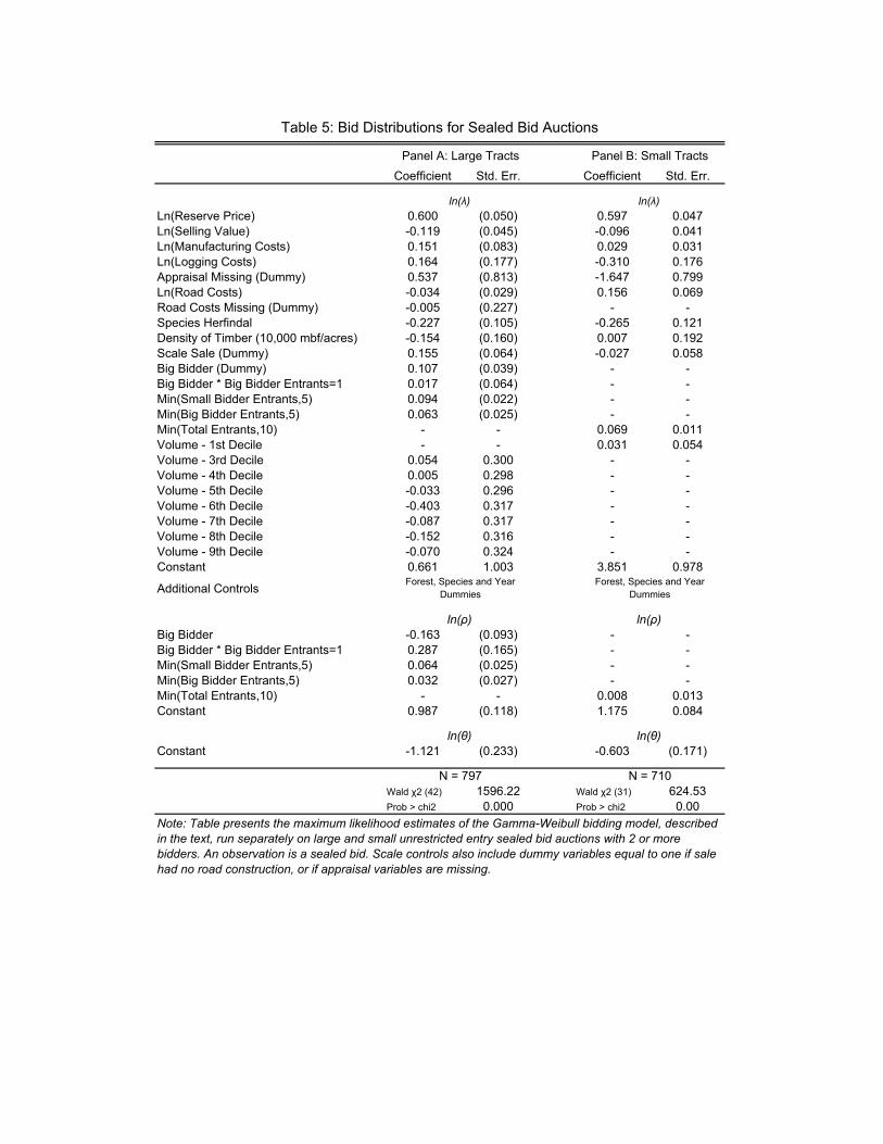
Table 5 reports estimated coe¢ cients of the bid distribution parameters (the summary

statistics for the estimation sample are reported in Appendix Table A2). There is strong

evidence for unobserved auction heterogeneity, indicated by the estimated variance parameter

�. In the larger sales, the bids of the big �rms stochastically dominate those of the small

�rms. Bids are also increasing in the number of competitors.

Given estimates of the equilibrium bid distributions, we follow Guerre, Perrigne and

Vuong, and Krasnokutskaya, in inferring the bidders�value distributions. If the bids in the

data are generated by equilibrium bidding, then in an auction with characteristics (X; u; n) a

bidder i�s bid bi and his value vi are related by the �rst order condition for optimal bidding:

vi = �i(bi;X; u; n) = bi +1P

j2nnigj(bijX;u;n)Gj(bijX;u;n)

: (3)

Having estimated each Gj, the only di¢ culty in inferring values is that we do not observe the

13Athey, Levin and Seira discuss the motivation both for using a parametric model of the bid distributionsand for the speci�c choice of the Gamma-Weibull functional form. It is possible to test the appropriateness ofthe parametric assumption using Andrews�(1997) Conditional Kolmogorov test. Using this test, we cannotreject the null hypothesis that the parametric model accurately describes the data at a 27% level for bigsales, and at a 31% level for small sales.

14

unobserved sale characteristic u corresponding to each observed bid. We do, however, have

an estimate of its distribution, so we can infer the distributions FS(�jX; u) and FB(�jX; u)

for any value of u from the relationship:

F� (vjX; u) = G� (��1� (v;X; u; n)jX; u; n):

Two subtleties arise in this step. First, if bidders�value distributions are to be bounded,

the equilibrium bid distributions must be as well, in contradiction to our Weibull speci�ca-

tion. We follow ALS�s procedure and truncate the estimated bid distributions. Second, the

theoretical value distributions do not depend on the actual number of bidders n, but as is

typical in two-stage estimation of auction models, there is some variation in our estimated

distributions. There are several approaches to this problem. One is to average the estimated

value distributions obtained for di¤erent value of n. The problem is that this leads to an

average bid distribution that is more spread out than any one distribution, which in turn

leads us to infer unrealistically high markups. Instead, we use the estimated value distrib-

ution corresponding to nS = nB = 2, this being a particularly common entry combination.

To provide a rough sense of the relationship between bids and values, we calculate that with

two small entrants and two big entrants, the median sealed bid markup varies from 12.6%

to 14.2% depending on the size of the sale and the type of bidder. These �gures are compa-

rable to those reported in ALS, who used a somewhat di¤erent dataset that did not include

set-aside sales, but included salvage sales.

B. Bidder Pro�ts as a Function of Entry and Sale Characteristics

Given the estimated value distributions, we can �nd bidder pro�ts as a function of

(X; u; n) by simulating either open or sealed bid auctions. The simulation procedure works

as follows. We �rst use the estimated value distributions, FS(�jX; u; n) and FB(�jX; u; n) to

compute the expected pro�ts of a small and big entrant as a function of (X; u; n). This

step is straightforward for an open auction because the equilibrium strategy is simply to bid

one�s value, so expected outcomes can be calculated by repeatedly drawing bidder values and

calculating auction outcomes. For sealed bid auctions, the simulation is similarly straightfor-

ward because we have already estimated the inverse equilibrium bid functions �S; �B above

15

(as described in equation (3)).

Given estimates of the pro�t functions �S (X; u; n) and �B (X; u; n) we average over

values of u, according the estimated distribution GU . This gives us the expected small and

big bidder pro�ts �S (X;n) and �B (X;n) that are relevant for the entry decision. (The

expected pro�ts also depend on whether a sale is open or sealed bid, but this will not be

made explicit unless necessary.) For the small sales, the expected pro�ts of small and big

entrants are the same, due to the symmetric value distributions. For the larger sales, big

bidders have higher expected pro�t. For example, in a large open auction with two small

and two large bidders, the expected pro�t of a big bidder is 2.94 times the expected pro�t

of a small bidder; the ratio is 2.83 in a sealed auction.

C. Potential Entrants, Entry Probabilities and Entry Cost

We next estimate the bidder entry costs for each sale, using the assumption that observed

entry patterns follow a type-symmetric equilibrium. To do this, we �rst need to estimate

the number of potential small and big entrants at each sale. We assume that potential

small bidder entry at a given sale is equal to the maximum small bidder entry observed

across all the unrestricted sales in the same forest-year. We can do somewhat better for

the big bidders because for the larger sales in our sample, the asymmetry of the estimated

value distributions implies that if small bidders are entering with positive probability, as we

observe, then big bidders must be entering with probability one. So for larger unrestricted

sales, we set the number of potential big bidders equal to the number of actual big entrants.

Then for the remaining sales, we assume that the number of potential big bidders equals the

number of actual big entrants in the �most similar� larger unrestricted sale, where �most

similar�means the sale in the same forest-year that is closest in timber volume.

To estimate entry costs, we use the equilibrium entry condition for small bidders. At

a type-symmetric equilibrium with 0 < pS < 1, these bidders are just indi¤erent between

entering and not entering. Denoting potential entry as N = (NS; NB), and writing the entry

cost as K(X), the indi¤erence condition is:

Xn�N

�S (X;n)Pr[njX;N; i 2 n] = K(X): (4)

16

Here Pr[njX;N; i 2 n] is the probability that n = (nS; nB) bidders enter given that i

enters. Assuming i is a small bidder,

Pr[njX;N; i 2 n] = Pr[nBjX;N ] � Pr[nSjX;N; i 2 n] (5)

= Pr[nBjX;N ] ��NS � 1nS � 1

�pS

nS�1 (1� pS)NS�nS . (6)

That is, the number of small entrants follows a binomial distribution where each of i�s

opponent�s independently decides to enter with probability pS. The big entrants either

enter with probability one (so nB = NB) if the sale is large and the value distributions are

asymmetric, or enter independently with probability pB = pS if the sale is small and the

value distributions are symmetric.

We estimate the equilibrium entry probability pS using the observed data on small bidder

entry, using the following parametric model:

pS(X;N) =exp(X�X +N�N)

1 + exp(X�X +N�N): (7)

Table 6 reports the maximum likelihood estimates of the entry probability parameters. Using

our estimates of pS (X;N), combined with the estimated pro�t function �S (X;n), we use

equation (4) to infer entry costs for all sales as a function of their covariates (X;N). We

estimate entry costs that are relatively high, $15,754 for the median sale.

As noted above, our empirical model of entry assumes a type-symmetric equilibrium

with mixed strategy entry by small bidders. In an earlier version of the paper, we based our

estimation on the assumption of a pure strategy entry equilibrium. The di¢ culty with that

approach is that we identi�ed many sales where it appeared that a single additional small

bidder entrant could make substantial pro�t by entering unless entry costs were very high.

In the context of a pure strategy equilibrium, a natural way to rationalize this might be to

assume that the set of potential entrants in such a sale had been exhausted. We found it

di¢ cult to get the data to separately distinguish high entry costs from a smaller number of

potential entrants, and hence hard to avoid estimating entry costs that seemed implausible

without making assumptions about the set of potential entrants that substantially a¤ected

17

our results. The mixed equilibrium model, despite having its own potential shortcomings,

avoids some of these problems because it assigns positive probability to sales having ex post

the feature that an extra small bidder could enter and make a positive pro�t.

5. Analysis of Set-Asides and Subsidies

In this section, we use the estimated model to analyze the set-aside program, and to

evaluate whether a subsidy program could achieve the government�s distributional goals at

lower cost in terms of revenue and e¢ ciency.

A. Assessing the Fit of the Model Inside and Outside the Estimation Sample

We use our model to predict the outcome of a small business set-aside auction and an

unrestricted auction for each tract in our data sample. For the subset of tracts where the

actual sale was unrestricted, we compare the model�s prediction for an unrestricted auction

to assess the model�s �t in-sample.14 For the tracts where the actual sale was a set-aside,

we compare our prediction of the set-aside outcome as a way to assess the model�s ability

to make out-of-sample predictions. (Note that by out-of-sample, we mean both on tract

characteristics and entry restrictions � the model was estimated only using the unrestricted

sales.) Throughout, we hold �xed the auction format: we simulate sealed bid auctions if a

tract was sold by sealed bidding, and open auctions if a tract was sold by open auction.

The results are reported in Table 7, which is divided into two panels. The �rst reports

average auction outcomes for the tracts that were sold in unrestricted sales. The second

reports the same outcomes for small business set-aside tracts. In each case, we report

the sale outcomes observed in the data, and the model�s predicted outcomes from running

the sales in unrestricted fashion and as small business set-asides. Comparing the �rst and

second columns in the top panel illustrates the model�s �t in-sample: predicted prices and

the percentage of sales won by small bidders are within 4% of the actual value.

The more challenging test for the model is the out-of-sample �t for tracts that were

sold as set-asides. The results can be seen by comparing the �rst and third columns of the

14Note that the bidder value distributions are estimated only on the sealed bid unrestricted sales, but theequilibrium entry probabilities are estimated using both open and sealed bid unrestricted sales.

18

bottom panel. The model predicts entry within 5% of the actual value, and prices and the

percentage of sales won by small bidders (rather than left unsold) within 2%. We also test

whether the predicted sealed bid distribution from the model matches to actual distribution

of sealed bids. To do this, we use the model to simulate the set-aside sales, then compare the

deciles of the simulated distribution of bids to the deciles of the observed bid distribution.

We construct standard errors for this test statistic using a bootstrap method.15 The p-value

associated with this test is 0.52, and the null hypothesis of equality of deciles is not rejected.

B. Assessing the Impact of Set-Asides

Table 7 also illustrates the impact of the set-aside policy on revenue, entry and welfare.

For the sales that were in fact set-asides, the model suggests that opening up entry would

have resulted in around 1.71 big bidders per sale, with 1.93 fewer small entrants. The fraction

of sales won by small bidders would have dropped to 51%, but revenue would have been 6%

higher, and surplus 21% higher. The model yields roughly similar predictions for the e¤ect

of a set-aside on the tracts that were sold in unrestricted fashion. A set-aside would have

reduced the entry of big �rms to zero, and the model suggests that the increase in small

bidder entry would have almost fully compensated in terms of revenue, leading to only a 3%

revenue loss. The predicted surplus loss is greater however, at 16%. These results are driven

mostly by the improved e¢ ciency in allocation. The reduced entry costs from unrestricted

sales contribute around 16% of the gain in surplus.

As previously noted, decreasing the number of potential bidders can in principle increase

participation and revenue when bidders play mixed strategies. One way to assess the quan-

titative importance of this e¤ect is to reduce the number of potential small bidder entrants

by one and recompute the entry equilibria and outcomes. If a signi�cant coordination e¤ect

is present, this should increase prices or entry. This is not what we �nd: overall small bidder

entry fell as a result of removing a potential small bidder, from 2.65 to 2.59. Prices also fell,

from 94.90 to 94.50. The coordination e¤ect does not appear to be very imporant in our

estimated model.15To construct a variance-covariance matrix for the observed bid deciles, we resample from the set of set-

aside sales and use the bid distributions from each resampled dataset. For the predicted sales, we resamplefrom the asymptotic distribution of the parameter estimates, and for each draw, re-do the simulation of theset-aside sales.

19

C. Assessing the Impact of Subsidies

We next use the model to consider an alternative small-business subsidy policy that

might substitute for the set-aside program. In particular, we consider a policy under a small

businesses would pay only 1=(1 + �) of its bid if it won an auction. We ask whether there

are values of � for which the Forest Service could increase revenue and economic e¢ ciency

while selling the same fraction of timber to small businesses.

To simulate the e¤ect of subsidies, we use essentially the same procedure as described

in the previous section. There is, however, an important quali�cation. Because the equilib-

rium sealed bidding strategies in a subsidized auction do not correspond to objects that we

observe directly in the data, we need to compute them. Computing equilibrium strategies

in asymmetric auctions is well-known to be a challenging problem (Marshall et al., 1994;

Bajari, 2001). The approach we take is to solve for equilibrium bidding strategies in an

auction in which the bid space is discretized and use this to approximate the equilibrium

in the underlying game with a continuous bid space. The details of the computation are

provided in Appendix B, and are perhaps of some independent interest. The validity of the

approximation derives from Athey (2001), who shows that for a class of auction games that

includes our model, the equilibria of auctions in which the bidding range is divided into a

grid converge to an equilibrium of the continuous bid space game as the grid becomes �ner.

We then compute entry equilibria. In the smallest sales, there may be multiple type-

symmetric equilibria. Absent subsidies, small and big bidders have identical valuation distri-

butions. We consider the natural symmetric equilibrium in which all potential bidders enter

with the same probability. With small bidder subsidies, we compute all type-symmetric

entry equilibria, and report average outcomes over these equilibria.

Table 8 shows expected outcomes, averaged over all auctions in the sample, and then

with the smallest sales broken out, for 6 di¤erent subsidy levels (no subsidy or � = 5,6,10,15

and 20%). The model�s predicted outcomes can be compared to the actual outcomes, which

are also reported in the table. The �rst point to make is that a relatively low subsidy level,

no more than 6%, appears su¢ cient to ensure that small businesses win the same fraction of

sales and volume of timber as under the observed set-aside policy. The second point is that in

our simulations, these subsidies increase revenue and e¢ ciency over existing policy. In fact,

20

revenue is increasing in the subsidy level, at least up to a 20% subsidy. The revenue e¤ect

arises because the subsidy makes small �rms more competitive in the large sales (partially

mimicking the allocation rule of an optimal auction), with the additional e¤ect of increasing

small business participation. The model predicts that a 6% subsidy would increase average

small business participation in the larger sales from 2.82 to 3.04.

A third point that comes out of the simulation results is that there appear to be subsidy

levels that result in fairly widespread bene�ts relative to the set-aside policy. For example,

a 6% subsidy entails more total surplus than the observed set-aside policy and almost no

surplus loss relative to the no-subsidy, no set-aside case. This subsidy level also results

in slightly more sales and timber won by small �rms, greater small bidder pro�ts, greater

revenue, and almost as great big bidder pro�ts as the set-aside policy. Larger subsidies

reduce e¢ ciency further, in part by encouraging excessive entry. Conditional on entry,

small subsidies induce small e¢ ciency costs: in an open auction, for example, the allocative

ine¢ ciency is bounded above by the level of the subsidy. Overall, however, the distortions

created by a subsidy policy appear to be relatively small compared to the costs of excluding

high-value big �rms from set-aside sales.

Fourth, we examine whether the bene�ts of subsidies can be approximated by using a

better-designed set-aside policy. Since the evidence suggests that small bidders are attracted

to small sales, we �rst consider a program that allocates all of the smallest sales to be set-

asides. However, the volume-based approach leads to lower e¢ ciency and revenue than the

existing set-aside program. We then consider a more sophisticated alternative. We predict

the sales that would be most e¢ cient to designate as set-asides given the constraint that

small bidders win as much volume as in the existing program. To do this, we select the

sales that have the �tted values closest to zero in a regression of (Unrestricted Surplus -

Set-Aside Surplus)/(Unrestricted Small Bidder Volume - Set-Aside Small Bidder Volume)

on tract characteristics, selecting just enough sales so that the volume constraint is satis�ed.

This approach leads to outcomes almost as e¢ cient as subsidies. Revenue is approximately

the same as if there were no preference program at all. Compared to the 6% subsidy, this

set-aside policy results in 3% less revenue, 11% less small bidder pro�t, and 8% more big

bidder pro�t.

21

Table 9 decomposes the impact of subsides and set-asides into bidding and participation

e¤ects. We �nd that for sales that were sold as set-asides, endogenous entry reduced the

loss in surplus (over an unrestricted policy) from 28% to 17%, and it reduced the revenue

losses from 30% to 5%. For �xed entry, a 5% subsidy has much less dramatic e¤ects on price

and surplus than a set-aside. Endogenous entry is thus less important in subsidized sales

than set-asides, although it is responsible for most of the change in revenue: The 5% subsidy

policy increases revenue over the unsubsidized case, due in part from shifting the allocation

to the small bidders conditional on entry, but mainly from encouraging more small bidder

entry.

Are there any weaknesses of subsidy policies? One is that the subsidy level must be

carefully chosen, but our results suggest that a wide range of subsidy levels improve over

current policy. Another concern is that setting aside a certain fraction of timber guarantees

that a minimum amount will be won by small businesses. A subsidy policy does not provide

a �rm guarantee. This concern may be particularly salient in a one-o¤ auction setting, such

as a sale of radio spectrum. But with many similar sales, it may be less important. To assess

this, we used the model to compute the probability distribution of the timber volume won by

small businesses in the 1330 sales in our data under the observed set-aside policy and under

a 6% subsidy. The cumulative distributions functions are shown in Figure 1. Because of the

guarantee that set-asides provide, the 6% subsidy CDF cannot quite stochastically dominate

the set-aside CDF. Nevertheless, Figure 1 shows that the relation between the CDFs is very

nearly one of stochastic dominance. It is very unlikely that under this subsidy loggers win

less than the quantity guaranteed to them by set-asides. Considering features of outcome

distributions other than the means does not much alter the basic picture: set-asides appear

to be a relatively expensive way to achieve distributional goals.

6. Subsidies and Optimal Auction Design

Our results on subsidies can be connected usefully to the theory of optimal auction design.

The connection is easiest to see with �xed participation. Suppose that a sale attracts some

combination of big and small bidders, N in total. Recall that if bidder i is of type � 2 fS;Bg

22

and has value v, its �marginal revenue�is MRi (v) = v� 1�F� (v)f� (v)

: Let v = (v1; :::; vN) denote

the vector of bidder values, and let qi (v) denote the equilibrium probability that i wins as

a function of the values. (Generally qi will be zero or one, unless there are ties or a random

allocation.) Of course, qi may depend on the size of the bidders, the auction format, and

whether a subsidy is in place.

Standard results from auction theory relate the allocation rule q1; :::qN and the mar-

ginal revenue functions MR1; :::;MRN to the expected surplus and revenue from the auc-

tion. In particular, expected auction surplus is Ev [P

i qi (v) � vi], while expected revenue is

Ev [P

i qi (v) �MRi (vi)]. In general, shifting the allocation toward bidders with higher value

increases expected surplus, while shifting the allocation toward bidders with higher marginal

revenue increases expected revenue. An e¢ cient auction awards the sale to the bidder with

the highest value � so qi = 1 if and only if vi � vj for all j. A revenue optimal auction

awards the sale to bidder i if and only if MRi (vi) �MRj (vj) for all j, and MRi (vi) � 0.

Figure 2 represents di¤erent allocations in the space of bidder valuations, assuming a

tract with average characteristics (X = X, u = 1). The x-axis represents the highest small

bidder valuation, and the y-axis the highest big bidder valuation. The forty-�ve degree line

represents the e¢ cient allocation: the high-value small bidder should win if and only if its

value is greater than that of the high-value big bidder. The left-most curve describes the

revenue-maximizing allocation, which favors small bidders. For all points to the right of the

curve, the high-value small �rm has the highest marginal revenue, so shifting the allocation

from the forty-�ve degree line toward the revenue-maximizing allocation reduces e¢ ciency

but increases revenue.

The remaining curves in Figure 2 describe the equilibrium allocations from open and

sealed bid auctions with no subsidy and with a 6% small bidder subsidy. (The open auction

allocations do not depend on the number of bidders; the sealed allocations assume two small

and two big bidders.) An open auction with no subsidy yields an e¢ cient outcome. Both a

shift to sealed bidding and a small bidder subsidy shift the allocation toward small bidders.

Both changes increase revenue at some cost to e¢ ciency. To �rst order, however, a small

shift away from the e¢ cient allocation matters more for revenue, helping to explain why the

revenue boost from a subsidy dominates the e¢ ciency loss in Table 8.

23

Figure 2 also shows that in the range of likely valuations (the deciles of the high bidder

value distributions are plotted on the axes), the subsidy has a larger e¤ect on the allocation

than moving from open auctions to sealed bidding. This helps to explain why ALS found

relatively minor e¤ects of shifting between open and sealed bidding under competitive bid-

ding, while we �nd larger e¤ects from modest subsidies. Of course, a set-aside policy has

even more dramatic consequences because it shifts the allocation to coincide with the y-axis

� reducing both e¢ ciency and revenue if small �rm participation is held constant.

A �nal point concerns endogenous participation. Suppose that we start from a situation

where equilibrium involves the big bidders entering with probability one and the small bidders

mixing. Because small bidders make lower expected pro�ts conditional on entry, shifting the

allocation in their favor will increase small bidder participation without decreasing the big

bidder participation, at least for small changes in the allocation. Now, in the unsubsidized

open auction case, equilibrium entry is e¢ cient. So if we shift to the small bidder subsidy

case, it follows that endogenous entry will tend to reinforce both the increase in revenue and

the reduction in surplus. This helps to clarify the �ndings reported in Table 8. Figure 2 also

show the revenue-optimal allocation rule with endogenous entry, which involves a larger bias

toward small bidders than the 6% subsidy.

7. Conclusion

Distributional objectives are an important feature of public sector procurement and nat-

ural resource sales. They can be achieved in a variety of ways, with subsidies and set-asides

being perhaps the two most common. Economic theory is not dispositive on which approach

can achieve a given distributional goal at lower social cost. Our estimates from the federal

government�s timber sales program, however, provide an example where set-asides might in

practice be relatively costly compared to a subsidy policy. The logic underlying our results is

that if the goal is to favor a signi�cantly weaker set of bidders, it may be better to subsidize

the weaker bidders and modestly tip outcomes across a broad range of sales, rather than

setting aside a targeted number of sales and precluding e¢ cient �rms from entering. Of

course, a quali�cation of our results is that they are obtained from a relatively small data

24

sample and a particular federal program. It would be interesting to explore whether there

are larger classes of public sector procurement or resource sale problems where similar results

obtain.

25

References

Andrews, Donald W.K., �A Conditional Kolmogorov Test,�Econometrica, 1997, 65(5),pp. 1097-1128.

Athey, S, �Single Crossing Properties and the Existence of Pure Strategy Equilibria inGames of Incomplete Information,�Econometrica, 2001, 69(4), pp. 861-889.

Athey, S. and P. Haile, �Identi�cation in Standard Auction Models,� Econometrica,2002, 70(6), pp. 2107-2140.

Athey, S. and J. Levin, �Information and Competition in U.S. Forest Service TimberAuctions,�Journal of Political Economy, 2001, 109(2), pp. 375�417.

Athey, S., J. Levin and E. Seira, �Comparing Open and Sealed Bid Auctions: Evidencefrom Timber Auctions,�Quarterly Journal of Economics, 2011, 126(1).

Ayres, I. and P. Cramton, �De�cit Reduction through Diversity: How A¢ rmativeAction at the FCC Increased Competition,� Stanford Law Review, 1996, 48(4), pp.761�815.

Bajari, P., �Comparing Competition and Collusion: A Numerical Approach,�EconomicTheory, 2001, 18(1), pp. 187-205.

Baldwin, L., R. Marshall, and J.-F. Richard., �Bidder Collusion at U.S. Forest ServiceTimber Auctions,�Journal of Political Economy, August 1997, 105(4), pp. 657�699.

Brannman, L., and L. Froeb, �Mergers, Cartels, Set-Asides and Bidding Preferences inAsymmetric Second-price Auctions,�Review of Economics and Statistics, 2000, 82(2),pp. 283-290.

Bulow, J. and P. Klemperer, �Prices and the Winner�s Curse,�Rand Journal of Eco-nomics, 2001, 33(1), pp. 1-21.

Flambard, V. and I. Perrigne, �Asymmetry in Procurement Auctions: Evidence fromSnow Removal Contracts, Economic Journal, 2006, 116(514), pp. 1014-1036.

Guerre, E., I. Perrigne and Q. Vuong, �Optimal Nonparametric Estimation of FirstPrice Auctions,�Econometrica, May 2000, 68(3), pp. 525�574.

Froeb, L. and P. McAfee, �Deterring Bid Rigging in Forest Service Timber Auctions,�U.S. Department of Justice Economic Analysis Group Working Paper, 1988.

Haile, P., �Auctions with Resale Markets: An Application to U.S. Forest Service TimberSales,�American Economic Review, June 2001, 92(3), pp. 399�427.

26

Haile, P., and E. Tamer, �Inference with an Incomplete Model of English Auctions,�Journal of Political Economy, 2003, 111(1), pp. 1-51.

Krasnokutskaya, E., �Identi�cation and Estimation of Auction Models with UnobservedHeterogeneity,�Review of Economic Studies, 2011, 78(1), pp. 293-327.

Krasnokutskaya, E. and K. Seim, �Bid Preference Programs and Participation in High-way Procurement Auctions,�American Economic Review, forthcoming.

Li, T. �Econometrics of First-Price Auctions with Entry and Binding Reserve Prices,�Journal of Econometrics, 2005, 126(1), pp. 173-200.

Li, T. and X. Zheng, �Entry and Competition in First-Price Auctions: Theory andEvidence from Procurement Auctions, Review of Economic Studies, 2009, 76, pp. 1397-1429.

Marion, J. �Are Bid Preferences Benign? The E¤ect of Small Business Subsidies inHighway Procurement Auctions,� Journal of Public Economics, 2007, 91(7-8), pp.1591-1624.

Marmer, V., A. Shneyerov and P. Xu, �What Model for Entry in First-Price Auctions:A Nonparametric Approach,�University of British Columbia Working Paper, 2010.

Marshall, R., M. Meurer, J.F. Richard and W. Stromquist, �Numerical Analysisof Asymmetric First-Price Auctions,�Games and Economic Behavior, 1994, 7, pp.193-220.

Maskin, E. and J. Riley, �Asymmetric Auctions,�Review of Economic Studies, July2000, 67(3), pp. 413�438.

McAfee, P. and J. McMillan, �Government Procurement and International Trade,�Journal of International Economics, 1989, 26, pp. 291�308.

Myerson, R., �Optimal Auction Design,�Mathematics of Operations Research, 1981, 6,pp. 58�73.

Roberts, J. and A. Sweeting, �Entry and Selection in Auctions,� Duke UniversityWorking Paper, 2010.

27

Unrestricted Set-Aside Unrestricted Set-Aside Unrestricted Set-AsideN

Mean Std. Dev. Mean Std. Dev. Mean Std. Dev. Mean Std. Dev. Mean Std. Dev. Mean Std. Dev.

Auction OutcomesPrices ($/mbf) 95.12 69.05 90.74 58.43 97.12 70.20 94.55 62.32 90.99 66.51 77.30 39.78Entrants 4.26 2.50 4.50 2.31 4.33 2.39 4.52 2.30 4.13 2.69 4.42 2.39 # Small Firms Entering 2.71 2.19 4.50 2.31 2.29 1.89 4.52 2.30 3.59 2.48 4.42 2.39 # Big Firms Entering 1.55 1.44 0.00 0.00 2.04 1.38 0.00 0.00 0.54 0.95 0.00 0.00Small Firm Wins Auction 0.52 0.50 1.00 0.00 0.37 0.48 1.00 0.00 0.85 0.36 1.00 0.00

Appraisal VariablesVolume of timber (100 mbf) 51.23 50.95 52.96 45.25 71.18 49.89 64.75 43.73 10.07 17.32 11.37 17.59Small Sale Dummy 0.21 0.41 0.14 0.35 0.04 0.21 0.03 0.18 0.54 0.50 0.53 0.51Reserve Price ($/mbf) 40.33 35.02 37.15 28.20 40.01 34.00 37.85 30.20 41.00 37.07 34.70 19.68Selling Value ($/mbf) 272.88 97.56 292.05 66.27 281.79 85.17 301.60 55.35 254.48 117.10 258.36 88.33Road Construction ($/mbf) 7.24 12.04 7.96 11.17 10.16 13.37 10.02 11.83 1.21 4.62 0.71 2.07Road Costs Missing 0.01 0.08 0.40 0.49 0.01 0.08 0.02 0.12 0.01 0.07 0.00 0.00Appraisal Missing 0.09 0.29 0.02 0.16 0.06 0.23 0.16 0.37 0.01 0.09 0.08 0.28Logging Costs ($/mbf) 102.87 40.99 109.94 32.93 107.22 36.50 114.06 30.59 93.88 47.79 95.40 37.03Manufacturing Costs ($/mbf) 121.97 46.01 127.76 34.76 127.55 38.08 132.42 26.39 110.45 57.47 111.33 52.25

Sale CharacteristicsContract Length (months) 24.25 14.95 27.87 14.26 30.32 13.75 31.51 13.55 11.72 7.86 15.00 7.87Species Herfindal 0.57 0.24 0.59 0.26 0.57 0.24 0.59 0.26 0.57 0.24 0.58 0.27Density of Timber (10,000 mbf/acre) 1160 1523 1130 1504 1070 1406 1006 1535 1346 1727 1569 1316Sealed Bid Sale 0.33 0.47 0.22 0.42 0.00 0.00 0.00 0.00 1.00 0.00 1.00 0.00Scale Sale 0.81 0.39 0.85 0.36 0.90 0.30 0.92 0.27 0.61 0.49 0.61 0.49Quarter of Sale 2.42 1.00 2.28 1.04 2.33 1.03 2.21 1.05 2.60 0.90 2.50 0.97Year of Sale 85.14 2.10 84.98 2.10 85.08 2.08 84.91 2.05 85.25 2.14 85.25 2.26Housing Starts 1597 257 1600 288 1602 261 1607 292 1588 250 1576 275

Local Industry ActivityLogging companies in county 20.00 18.59 22.11 24.97 21.33 19.39 22.33 24.51 17.24 16.52 21.33 26.89Sawmills in County 6.33 6.99 8.23 10.99 6.62 7.12 8.25 10.78 5.74 6.69 8.17 11.86Small Firms Active in Last Year 13.18 7.44 14.19 7.31 13.31 7.68 14.13 7.20 12.92 6.91 14.39 7.77Big Firms Active in Last Year 3.17 1.76 2.34 1.72 3.34 1.82 2.34 1.79 2.82 1.58 2.36 1.44

Note: Data includes non-salvage Forest Service sales in California between 1982 and 1989. Small firms are those that are eligible for small business set-aside sales. A sale is a "small sale" if it is in the lowest quintile by timber volume. Timber volume is measured in thousand board feet (mbf). The measures of local industry activity for a given sale include the number of logging companies and sawmills as reported in the US Census County Business Patterns, and the number of small and big firms that bid in the same forest-district within the prior year.

786 127

Table 1: Summary Statistics

All Sales

1167 163

Sealed Sales

381 36

Open Sales

Coefficient Std Err.Sealed Bids Per Quintile

Fraction of Unrestricted Sealed and Open Sales

Won by Small Firms

Big Firm Dummy x Sale in First Size Quintile -0.005 (0.071) 824 0.95 Sale in Second Size Quintile 0.111 (0.040) 752 0.77 Sale in Third Size Quintile 0.041 (0.102) 80 0.51 Sale in Fourth Size Quintile 0.028 (0.138) 46 0.41 Sale in Fifth Size Quintile 0.066 (0.144) 29 0.28

Total Number of Sealed BidsTotal Number of Auctions 1167

Table 2: Small and Big Firm Bidding Differences

Note: The first two columns report regression results where the the dependent variable is the logarithm of the bid per unit volume, the data includes all sealed bids submitted in unrestricted auctions, and the explanatory variables include auction fixed effects and a dummy equal to one if the bidder is a big firm interacted with the size of the sale. The sales are assigned to size quintiles based on the volume of timber being sold. The third column shows the number of unrestricted sealed bids for each size category. The fourth column shows the fraction of (sealed and open) unrestricted sales won by small firms.

1731417

Regression Model: Log(Bid)

Marginal Effect Std. Err.

Appraisal ControlsLn(Reserve Price) -0.009 (0.012)Ln(Selling Value) 0.039 (0.031)Ln(Manufacturing Costs) 0.012 (0.015)Ln(Logging Costs) -0.133 (0.041)Ln(Road Costs) 0.006 (0.006)Road Costs Missing (Dummy) 0.111 (0.144)Appraisal Missing (Dummy) -0.123 (0.028)

Other Sale Characteristicsln(Contract Length/volume) 1.382 (0.576)Species Herfindal -0.019 (0.031)Density of Timber (10,000 mbf/acres) 0.002 (0.045)Sealed Bid (Dummy) -0.012 (0.021)Scale Sale (Dummy) 0.013 (0.020)ln(Monthly US House Starts) 0.049 (0.080)

Volume Controls (Dummy Variables):Volume: 1.5-3 hundred mbf 0.017 (0.061)Volume: 3-5 0.089 (0.115)Volume: 5-8 0.062 (0.101)Volume: 8-12 0.051 (0.102)Volume: 12-20 0.028 (0.087)Volume: 20-40 0.168 (0.176)Volume: 40-65 0.161 (0.165)Volume: 65-90 0.175 (0.179)Volume: 90+ 0.051 (0.099)

Local Industry Activityln(Loggers in County) -0.010 (0.013)ln(Sawmills in County) -0.006 (0.011)ln(Active Small Firms) 0.031 (0.012)ln(Active Big Firms) -0.047 (0.009)

Additional Controls (Dummy Variables)Chi-Squared Statistics (p-value in parenthesis)Years 4.760 (0.690)Quarters 8.620 (0.035)Species 10.230 (0.115)Location 37.380 (0.000)

LR chi2 (52) 235.04P-value 0.00Pseudo-R2 0.24

N=1315

Table 3: Choice of Set-Aside Sale

Note: Table reports results from a logit regression where the dependent variable is equal to one if the sale is a small business set-aside. The estimates are reported as marginal probability effects at the mean of the independent variables.

(1) (2)Dependent Variable

coefficient s.e. coefficient s.e.

Average Effect (Full Sample) OLS with Interactions -0.127 (0.068) -0.102 (0.072)

Average Effect on Set-Aside Tracts OLS with Interactions 0.083 (0.050) -0.001 (0.045)

Table 4: Effects of Set-Aside Provision

ln(Entrants) ln(Revenue)

Note: Table reports estimates from OLS regressions of dependent variable on sale characteristics and a dummy variable for small business set-aside sale interacted with all characteristics. The first row shows the estimated average treatment effect of a set-aside for the full sample of sales. The second row shows the estimated effect for the set-aside tracts. Sale characteristics in the regression include all the variables from Table 3 and the estimated probability that the auction was conducted as a set-aside (the propensity score from the logit regression in Table 3).

Panel A: Large Tracts Panel B: Small TractsCoefficient Std. Err. Coefficient Std. Err.

Ln(Reserve Price) 0.600 (0.050) 0.597 0.047Ln(Selling Value) -0.119 (0.045) -0.096 0.041Ln(Manufacturing Costs) 0.151 (0.083) 0.029 0.031Ln(Logging Costs) 0.164 (0.177) -0.310 0.176Appraisal Missing (Dummy) 0.537 (0.813) -1.647 0.799Ln(Road Costs) -0.034 (0.029) 0.156 0.069Road Costs Missing (Dummy) -0.005 (0.227) - -Species Herfindal -0.227 (0.105) -0.265 0.121Density of Timber (10,000 mbf/acres) -0.154 (0.160) 0.007 0.192Scale Sale (Dummy) 0.155 (0.064) -0.027 0.058Big Bidder (Dummy) 0.107 (0.039) - -Big Bidder * Big Bidder Entrants=1 0.017 (0.064) - -Min(Small Bidder Entrants,5) 0.094 (0.022) - -Min(Big Bidder Entrants,5) 0.063 (0.025) - -Min(Total Entrants,10) - - 0.069 0.011Volume - 1st Decile - - 0.031 0.054Volume - 3rd Decile 0.054 0.300 - -Volume - 4th Decile 0.005 0.298 - -Volume - 5th Decile -0.033 0.296 - -Volume - 6th Decile -0.403 0.317 - -Volume - 7th Decile -0.087 0.317 - -Volume - 8th Decile -0.152 0.316 - -Volume - 9th Decile -0.070 0.324 - -Constant 0.661 1.003 3.851 0.978

Additional Controls

Big Bidder -0.163 (0.093) - -Big Bidder * Big Bidder Entrants=1 0.287 (0.165) - -Min(Small Bidder Entrants,5) 0.064 (0.025) - -Min(Big Bidder Entrants,5) 0.032 (0.027) - -Min(Total Entrants,10) - - 0.008 0.013Constant 0.987 (0.118) 1.175 0.084

Constant -1.121 (0.233) -0.603 (0.171)

Wald χ2 (42) 1596.22 Wald χ2 (31) 624.53

Prob > chi2 0.000 Prob > chi2 0.00

Table 5: Bid Distributions for Sealed Bid Auctions

ln(λ)ln(λ)

N = 797 N = 710

ln(θ)

ln(ρ) ln(ρ)

Forest, Species and Year Dummies

Forest, Species and Year Dummies

Note: Table presents the maximum likelihood estimates of the Gamma-Weibull bidding model, described in the text, run separately on large and small unrestricted entry sealed bid auctions with 2 or more bidders. An observation is a sealed bid. Scale controls also include dummy variables equal to one if sale had no road construction, or if appraisal variables are missing.

ln(θ)

Coefficient Std. Err. Coefficient Std. Err.

Ln(Reserve Price) -0.276 (0.054) -0.354 (0.079)Ln(Selling Value) -0.107 (0.079) 0.004 (0.061)Ln(Manufacturing Costs) 0.143 (0.089) 0.039 (0.064)Ln(Logging Costs) -1.637 (0.206) -1.290 (0.294)Appraisal Missing (Dummy) -7.307 (0.966) -6.252 (1.365)Ln(Road Costs) -0.136 (0.027) -0.102 (0.135)Road Costs Missing (Dummy) 0.190 (0.379) -2.304 (1.101)Species Herfindal -0.260 (0.146) -0.339 (0.220)Density of Timber (10,000 mbf/ac -0.332 (0.002) -0.754 (0.004)Scale Sale (Dummy) 0.236 (0.103) 0.453 (0.106)Potential Big Bidder Entrants = 0 0.144 (0.114) - -Min(Potential Big Bidder Entrants 0.132 (0.035) - -Potential Entrants -0.190 (0.017) -0.089 (0.032)Sealed 0.278 (0.100) - -Volume - 1st Decile - - -0.263 (0.106)Volume - 3rd Decile 1.242 (0.149) - -Volume - 4th Decile 0.928 (0.137) - -Volume - 5th Decile 0.501 (0.124) - -Volume - 6th Decile 0.521 (0.118) - -Volume - 7th Decile 0.221 (0.120) - -Volume - 8th Decile 0.191 (0.124) - -Volume - 9th Decile 0.212 (0.117) - -Constant 8.964 (1.093) 9.425 (1.722)

Additional Controls

Wald χ2 (42) 837.19 Wald χ2 (33) 178.27Prob > chi2 0.000 Prob > chi2 0.000

Note: Table presents the estimates from the binomial entry model, estimated separately on unrestricted large and unrestricted small tracts.

N = 925 N = 242

Table 6: Entry Probabilities for Unrestricted Auctions

Panel A: Large Tracts Panel B: Small Tracts

Forest, Species and Year Dummies

Forest, Species and Year Dummies

Actual Outcome Unrestricted Std. Err. Set-Aside Std. Err.

Avg. Small Bidder Entry 2.71 2.69 (0.03) 4.93 (0.36)Avg. Big Bidder Entry 1.55 1.57 (0.00) 0.00 (0.00)Avg. Total Entry 4.26 4.26 (0.03) 4.93 (0.36)Avg. Prices 95.12 98.51 (15.51) 95.87 (15.68)% Sales won by Small Bidders 52.44 54.14 (0.03) 97.93 (0.01)Avg. Sale Surplus (per mbf) 119.16 (25.85) 100.11 (19.52)

Avg. Small Bidder Entry 4.50 2.57 (0.05) 4.71 (0.32)Avg. Big Bidder Entry 0.00 1.71 (0.00) 0.00 (0.00)Avg. Total Entry 4.50 4.28 (0.05) 4.71 (0.32)Avg. Prices 90.74 97.29 (17.47) 92.01 (16.87)% Sales won by Small Bidders 100.00 50.63 (0.04) 98.28 (0.01)Avg. Sale Surplus (per mbf) 119.21 (29.11) 98.39 (22.00)

Note: Table reports actual outcomes for California sales and predicted outcomes generated by the model, assuming either that sales are unrestricted or conducted as set-asides. The predicted fraction of set-asides won by small bidders can be less than one because (a) for some unrestricted sales, there are no potential small entrants, and (b) the reserve price binds in some simulated auctions. The possibility for multiple entry equilibria means we obtain a range of predicted outcomes. We report the midpoints; the ranges are less than 0.5% around the reported numbers. Bootstrapped standard errors from 250 bootstrap repetitions are reported in parentheses.

Panel B: Tracts sold by set-aside sale (N=163)

Predicted Outcomes

Table 7: Effect of the Set-Aside Program

Panel A: Tracts sold by unrestricted sale (N=1167)

Outcome VariableSmall

Bidder EntryBig Bidder

Entry

Total Small Bidder Profit

($'000s)

Total Big Bidder Profit

($'000s)Price

($/mbf)Gross Price

($/mbf)

% Won by Small

BiddersTotal Small Bidder Vol.

Surplus (per mbf)

Actual Policy 2.94 1.38 72.78 188.46 97.72 97.72 59.55 2223.64 116.62Set-Asides Selected by Sale Volume 3.41 1.04 71.94 189.61 97.46 97.46 68.66 2184.34 113.05Predicted Optimal Set-Asides 2.86 1.46 67.39 199.14 98.66 98.66 58.95 2239.06 118.69No Subsidy 2.66 1.60 59.24 213.31 98.30 98.30 53.18 1817.95 119.315% Subsidy 3.04 1.59 72.84 189.39 101.40 103.07 58.46 2207.21 119.156% Subsidy 3.12 1.58 75.30 185.09 101.92 103.95 59.57 2277.82 119.0910% Subsidy 3.37 1.57 84.15 169.47 103.65 107.34 63.42 2534.93 118.7615% Subsidy 3.62 1.55 93.46 152.87 105.23 111.29 67.40 2809.66 118.2220% Subsidy 3.82 1.55 101.38 138.60 106.38 115.09 70.81 3043.15 117.58

Actual Policy 3.41 0.27 10.27 0.92 84.66 84.66 88.66 256.54 84.73Set-Asides Selected by Sale Volume 3.69 0.00 11.18 0.00 85.30 85.30 96.12 277.92 85.22Predicted Optimal Set-Asides 3.65 0.05 11.08 0.13 85.30 85.30 95.09 274.05 85.22No Subsidy 3.31 0.33 9.92 1.34 84.42 84.42 85.21 247.26 85.435% Subsidy 3.36 0.31 9.97 1.26 84.93 85.57 85.98 250.15 85.486% Subsidy 3.41 0.27 10.15 1.08 85.01 85.63 86.94 253.44 85.4910% Subsidy 3.51 0.17 10.44 0.79 85.25 85.79 89.46 260.97 85.5115% Subsidy 3.57 0.11 10.62 0.61 85.36 85.71 91.47 265.31 85.4620% Subsidy 3.62 0.07 10.93 0.29 85.46 85.64 93.27 270.16 85.44

Actual Policy 2.82 1.66 88.33 235.13 100.97 100.97 52.31 2713.11 124.55Set-Asides Selected by Sale Volume 3.34 1.30 87.05 236.79 100.49 100.49 61.83 2658.70 119.98Predicted Optimal Set-Asides 2.66 1.81 81.40 248.66 101.99 101.99 49.96 2728.01 127.02No Subsidy 2.50 1.91 71.51 266.05 101.76 101.76 45.22 2208.78 127.745% Subsidy 2.96 1.91 88.48 236.20 105.50 107.42 51.61 2694.17 127.536% Subsidy 3.04 1.91 91.51 230.87 106.12 108.51 52.76 2781.54 127.4510% Subsidy 3.34 1.91 102.49 211.44 108.23 112.70 56.94 3100.75 127.0415% Subsidy 3.63 1.91 114.07 190.76 110.18 117.65 61.41 3442.76 126.3720% Subsidy 3.87 1.91 123.88 173.02 111.58 122.42 65.22 3733.14 125.58

Note: Table reports outcomes, averaged over all auctions, of different set-aside and subsidy policies. The actual outcomes are those given the set-aside policy observed in the data. All set-aside policies shown acheive at least as much total small bidder volume over all sales as actual set-asides do. "Volume-Based Set-Asides" set aside those sales smaller than a volume threshold, where the volume threshold is set to achieve the overall small bidder volume target. "Predicted Optimal Set-Asides" are those sales which have the fitted values closest to zero in a regression of (Unrestricted Surplus - Set-Aside Surplus)/(Unrestricted Small Bidder Volume - Set-Aside Small Bidder Volume) on tract characteristics. 469 sales are set aside under volume-based set-asides, and 197 under predicted optimal set-asides. For the counterfactual subsidies, the subsidies are applied to every auction in the sample.

Table 8: Comparison of Set-Asides and Subsidies

Panel A: All Sales (N=1330)

Panel B: Small Sales (N=265)

Panel C: Large Sales (N=1065)

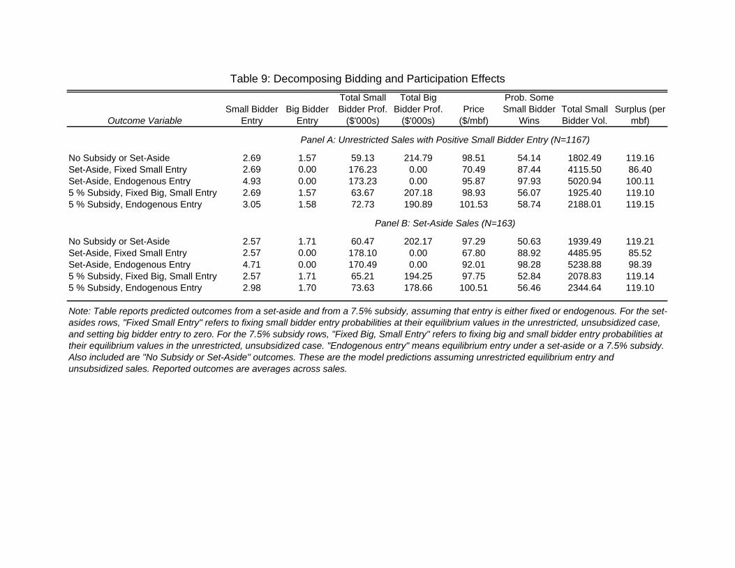
Outcome VariableSmall Bidder

EntryBig Bidder

Entry

Total Small Bidder Prof.

($'000s)

Total Big Bidder Prof.

($'000s)Price

($/mbf)

Prob. Some Small Bidder

WinsTotal Small Bidder Vol.

Surplus (per mbf)

No Subsidy or Set-Aside 2.69 1.57 59.13 214.79 98.51 54.14 1802.49 119.16Set-Aside, Fixed Small Entry 2.69 0.00 176.23 0.00 70.49 87.44 4115.50 86.40Set-Aside, Endogenous Entry 4.93 0.00 173.23 0.00 95.87 97.93 5020.94 100.115 % Subsidy, Fixed Big, Small Entry 2.69 1.57 63.67 207.18 98.93 56.07 1925.40 119.105 % Subsidy, Endogenous Entry 3.05 1.58 72.73 190.89 101.53 58.74 2188.01 119.15

No Subsidy or Set-Aside 2.57 1.71 60.47 202.17 97.29 50.63 1939.49 119.21Set-Aside, Fixed Small Entry 2.57 0.00 178.10 0.00 67.80 88.92 4485.95 85.52Set-Aside, Endogenous Entry 4.71 0.00 170.49 0.00 92.01 98.28 5238.88 98.395 % Subsidy, Fixed Big, Small Entry 2.57 1.71 65.21 194.25 97.75 52.84 2078.83 119.145 % Subsidy, Endogenous Entry 2.98 1.70 73.63 178.66 100.51 56.46 2344.64 119.10

Table 9: Decomposing Bidding and Participation Effects

Panel A: Unrestricted Sales with Positive Small Bidder Entry (N=1167)

Panel B: Set-Aside Sales (N=163)

Note: Table reports predicted outcomes from a set-aside and from a 7.5% subsidy, assuming that entry is either fixed or endogenous. For the set-asides rows, "Fixed Small Entry" refers to fixing small bidder entry probabilities at their equilibrium values in the unrestricted, unsubsidized case, and setting big bidder entry to zero. For the 7.5% subsidy rows, "Fixed Big, Small Entry" refers to fixing big and small bidder entry probabilities at their equilibrium values in the unrestricted, unsubsidized case. "Endogenous entry" means equilibrium entry under a set-aside or a 7.5% subsidy. Also included are "No Subsidy or Set-Aside" outcomes. These are the model predictions assuming unrestricted equilibrium entry and unsubsidized sales. Reported outcomes are averages across sales.

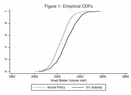
0 .2

.4.6

.8

1 Figure 1: Empirical CDFs

1800 2000 2200 2400 2600 2800 Small Bidder Volume (mbf)

Actual Policy 5% Subsidy

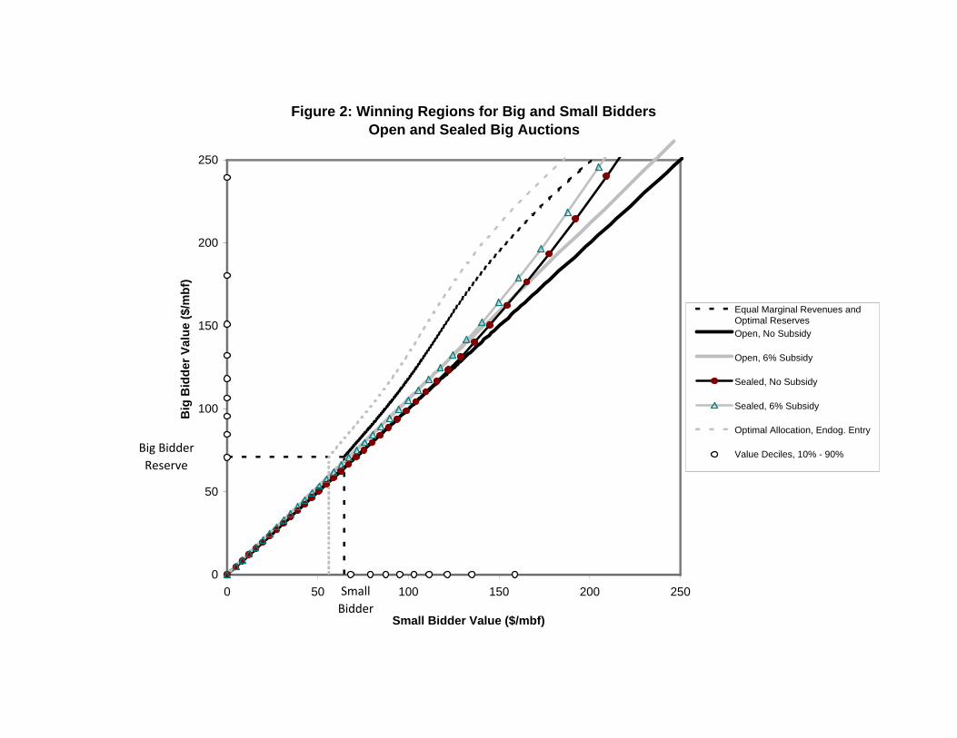
Figure 2: Winning Regions for Big and Small BiddersOpen and Sealed Big Auctions

0

50

100

150

200

250

0 50 100 150 200 250

Small Bidder Value ($/mbf)

Big

Bid

der V

alue

($/m

bf)

Equal Marginal Revenues andOptimal ReservesOpen, No Subsidy

Open, 6% Subsidy

Sealed, No Subsidy

Sealed, 6% Subsidy

Optimal Allocation, Endog. Entry

Value Deciles, 10% - 90%Big Bidder Reserve

Small BidderR

Figure 1. Shows the distribution of (per-sale) timber volume won by small bidders across simulations conducted using the actual set-aside policy and a 5% subsidy. To construct the figure, we simulated the whole set of auctions 800 times under each policy. For each simulation, we calculated the total timber volume won by small bidders and divided by the number of sales. The plot shows the distribution of this per-sale volume number. Figure 2. Shows the allocation from various subsidized and unsubsidized auctions. The x-axis is the highest value among the small bidders, and the y-axis the highest value among the large bidders. The dots on each axis show the deciles of the distributions of these high values. In each case, we assume two big bidders, eight potential small bidders, X equal to the mean among the larger tracts, and u=1. The sealed auction cases assume two actual small bidders. The first plot shows the Myerson revenue-optimal allocation with fixed entry, n=(2,2). The final plot shows the revenue-optimal allocation with endogenous equilibrium entry by the bidders.