Francesca Foliano, Francis Green and Marcello Sartarelli

Can Talented Pupils with LowSocio-economic Status Shine?Evidence from a Boarding Schoolad

serie

WP-AD 2017-05

Los documentos de trabajo del Ivie ofrecen un avance de los resultados de las investigaciones económicas en curso, con objeto de generar un proceso de discusión previo a su remisión a las revistas científicas. Al publicar este documento de trabajo, el Ivie no asume responsabilidad sobre su contenido. Ivie working papers offer in advance the results of economic research under way in order to encourage a discussion process before sending them to scientific journals for their final publication. Ivie’s decision to publish this working paper does not imply any responsibility for its content. La Serie AD es continuadora de la labor iniciada por el Departamento de Fundamentos de Análisis Económico de la Universidad de Alicante en su colección “A DISCUSIÓN” y difunde trabajos de marcado contenido teórico. Esta serie es coordinada por Carmen Herrero. The AD series, coordinated by Carmen Herrero, is a continuation of the work initiated by the Department of Economic Analysis of the Universidad de Alicante in its collection “A DISCUSIÓN”, providing and distributing papers marked by their theoretical content. Todos los documentos de trabajo están disponibles de forma gratuita en la web del Ivie http://www.ivie.es, así como las instrucciones para los autores que desean publicar en nuestras series. Working papers can be downloaded free of charge from the Ivie website http://www.ivie.es, as well as the instructions for authors who are interested in publishing in our series. Versión: octubre 2017 / Version: October 2017 Edita / Published by: Instituto Valenciano de Investigaciones Económicas, S.A. C/ Guardia Civil, 22 esc. 2 1º - 46020 Valencia (Spain) DOI: http://dx.medra.org/10.12842/WPAD-2017-05

3

WP-AD 2017-05

Can Talented Pupils with Low Socio-economic Status Shine? Evidence from a Boarding School*

Francesca Foliano, Francis Green and Marcello Sartarelli**

Abstract

We study whether substituting family with school inputs for high ability pupils with low socio-economic status (SES) has an impact on achievement in the compulsory school final exams using administrative data on England. By considering a selective secondary, well-resourced boarding school admitting an unusually high share of talented pupils with low SES, we estimate the effect with propensity score matching to obtain comparable control groups in selective day schools. Our main finding is that the probability of being in the top decile of achievement in the exams increases by about 17 percentage points compared to 59% for controls, i.e. by 29%.

Keywords: ability, achievement gap, boarding, education, grammar school, GCSE, private school, socio-economic status, SES.

JEL classification numbers: I21, I24, I32, J62.

* We thank Pedro Albarran, Marianna Battaglia, Richard Dorsett, Amanda Gosling, Iñigo Iturbe, Steve Machin, Giuseppe Migali, Olmo Silva, Tanya Wilson and participants at the Universidad de Alicante Applied Seminar, University of Kent Research Seminar, AEDE 2014, SIEP 2016 and RES 2017 for their useful comments. We also thank the management of Christ Hospital School for kindly providing us with information about the school’s admissions criteria and procedures. The responsibility for the findings in this paper are entirely our own. Financial support from the ESRC (Grant No. ESJ0191351), Spanish Ministerio de Economía y Competitividad (ECO2016-77200-P, ECO2015-65820-P and ECO2013-43119) and Universidad de Alicante (GRE 13-04) is gratefully acknowledged.

** F. Foliano: University of Kent and NIESR. F. Green: UCL Institute of Education. M. Sartarelli: Universidad de Alicante, e-mail: marcellosartarelli@gmail.com (corresponding autor).

1 Introduction

Achievement gaps by socio-economic status (SES) are a policy challenge worldwide(see for a review Sirin, 2005; Reardon, 2011). In England they are observed as earlyas primary education and are either constant or tend to increase with age (Deardenet al., 2011). While gaps by SES tend to be concentrated among pupils who areinitially low achievers, they have also been recently observed among high achievers(Crawford et al., 2014; Jerrim, 2017). This may have potentially high opportunitycosts if pupils who seem to have the potential to perform well at school, which is agood predictor of success in the labour market in adulthood, are held back or sloweddown by low SES.

Most of the policies that have been designed to counteract the low SES neg-ative influence on pupils’ achievement compensate poor family inputs with betterschool inputs. Their impact on children’s achievement is studied theoretically andempirically by letting the family and the school be inputs in the child’s educationalproduction function (Todd and Wolpin, 2003, 2007). However, the effect of a schoolpolicy may be confounded by family inputs, that are not easily observed. Familyinputs might reinforce the role of school policies if parents respond by putting moreeffort into their children’s development and vice versa dilute it if they put less.1

Boarding schools offer, instead, a suitable example of substantial substitutionof family inputs for school inputs, i.e. they reduce the role of family inputs for allpupils, since they offer education during the day and lodging at night in weekdays.However, obtaining clean estimates of the effect of attending a boarding school on,for example, pupils’ achievement is an empirical challenge as it may be confoundedby a selection effect if boarding schools pupils and pupils in other schools differsubstantially in ability or in SES.

Lotteries granting random admission to oversubscribed boarding schools havebeen used to obtain clean estimates of the effect of attending a boarding school. Ran-domly admitted pupils obtain substantially higher tests scores than non-admittedones in boarding schools in poor neighbourhoods in the US (Curto and Fryer Jr,

1Recent examples of school policies are the introduction of sponsored Academy schools indisadvantaged areas in the UK (Eyles et al., 2016) and of Charter schools in the US (see a reviewin Epple et al., 2016), as well as more narrowly targeted interventions in urban schools in the UK,such as Excellence in the Cities (Machin et al., 2004). Exceptionally, the Assisted Places Scheme,which ran in the UK from 1981 to 1997 with mixed success, involved some boarding schools,though only a minority of scheme participants were from disadvantaged backgrounds (Whitty andEdwards, 1998).

14

2014). Related research also exploiting random admission in an elite school in Franceobtains similar results (Behaghel et al., 2017). Lotteries offer the advantage thatadmitted pupils have similar characteristics to those not admitted. However, theestimated effect may be biased upward since oversubscribed schools, the only onesin which lotteries are run, may be on higher demand than other schools becausethey are of higher quality (Eyles and Machin, 2015). In addition, the low number ofobservations limits the possibility to study the impact of boarding for high achieverswith low SES.

This paper is the first to test the hypothesis that offering high achievers with lowSES admission at a truly selective boarding school, whose name is Christ Hospital(CH hereafter), leads to higher achievement (H1). We use rich administrative dataon England and measure achievement at age 7, 11 (Key Stage 1 and 2) and in thecompulsory school final exams at age 16 (General Certificate of Secondary Educa-tion, GCSE hereafter) for five consecutive cohorts of pupils. The aim of our researchdesign is to find for each pupil at CH a pupil in a selective day school who is assimilar as possible in observable characteristics by using propensity score matching.We use the following two measures of SES: the income deprivation affecting chil-dren index (IDACI), measuring the share of children in low income households bylocal area, and, in addition, whether pupils’ parents obtain income support from thegovernment, proxied by whether pupils are eligible for Free School Meals (FSM).

We also test whether there is heterogeneity in the impact of CH on achievement asa related hypothesis (H2). We study whether it differs for pupils with very low SES,proxied by an IDACI greater than the median value, to assess if they are the oneswho benefit most from CH as their learning environment is the one improving themost upon admission. In addition, we examine the effects of CH separately for girlsand boys given that the home environment’s contribution to academic achievementmay be gendered and in light of the widely documented achievement gap in favourof girls in England (Machin and McNally, 2005).

CH is an outlier in English private education, in that it educates a very highshare of high achievers with low SES. Its especially wealthy foundation enablesit to admit the majority of its pupils with low or no fees through means-testedbursaries. Since it is selective and boarding, we compare its pupils with those in thefollowing two types of selective day schools, i.e. our control groups. The first arepupils in grammar schools, that are highly selective state schools with substantiallyfewer resources than CH. The second group are pupils in independent schools, that

25

are also well-resourced like CH, although they tend to be less selective based onacademic merit. In addition, in our control groups we only selected pupils fromprimary schools located in the same local authority as those attended by pupils whothen went to CH. This ensures that the school and non-school environment that apupil at CH and a very similar pupil in a selective day school experienced beforesecondary school is also comparable.

We find that pupils’ achievement at CH is significantly higher than for controlpupils (H1). The probability of at least five GCSE exams (GCSEs hereafter) atA-A*, i.e. of being in the top decile in the distribution of the number of GCSEs atA-A*, is significantly higher at CH by 17.4 and 12.6 percentage points, i.e. a 20-29%increase with respect to 59-64% for matched pupils in grammar and independentday schools respectively. When we assess whether there is heterogeneity in ourmain results (H2), we find that they tend to be driven by higher point estimatesfor pupils from poorer areas, proxied by an IDACI level above the median, and forgirls. Crucially, predetermined characteristics for pupils at CH and for controls ingrammar and independent schools are balanced and, in addition, our main resultsare robust to a set of sensitivity checks.

To the best of our knowledge, our results are the first in showing that a board-ing school admitting high ability and low SES pupils significantly improves theirachievement (H1). They contribute to the school choice literature by suggestingthat currently available alternatives to standard schooling options may play a rele-vant role in reversing the achievement gap for these pupils. Finding that the impactis higher for poor pupils (H2) also contributes to studies on children’s educationalproduction function by suggesting that the substitutability between the inputs thatthese pupils obtain from parents and from the school is not substantially dilutedby economic, cognitive or psychological disadvantages associated with low SES. Ourrelated finding on the greater effect for girls is also relevant for an understanding ofthe gender achievement gap for high ability pupils in England. Finally, our resultscontribute to the recent policy debate over the use of boarding schools for disadvan-taged children in England (Department for Education, 2014, 2016) that so far lacksa thorough quantitative economic analysis.

The rest of the paper is structured as follows. Section 2 reviews the relevantliterature. Section 3 describes the institutional setting of compulsory education inEngland and the data that we use in the empirical analysis. Section 4 outlines theeconometric strategy. Section 5 describes the main results, section 6 reports the

36

results of a sensitivity analysis and, finally, section 7 discusses them and concludes.

2 Literature review

In this section, we consider what existing studies around the world reveal aboutthe effects of boarding on academic and non-academic outcomes. In the US, inrecent years, boarding secondary schools for bright pupils with low SES have beenintroduced. SEED schools in Washington and Baltimore are the only urban publicschools that combine the charter school model with a 5-day-a-week boarding pro-gram in poor neighbourhoods. Curto and Fryer Jr (2014) estimate the impact ofattending a SEED school in Washington on achievement by exploiting lottery-drivenadmission that is used when a school is oversubscribed. By comparing achievementof students admitted and of those turned down by the lottery, they find that SEEDincreases achievement by about 20% of a standard deviation in reading and in math,with results being mainly driven by females.

Similarly, in France public ‘boarding schools of excellence’ for poor and highachieving pupils have been opened in deprived suburbs of large French cities. Be-haghel et al. (2017) exploit an admission lottery to study the effect of attending onesuch school in the suburbs of Paris. They find that by the end of the first year,achievement in French and in maths is lower (60-270%) although differences are notsignificant. A subjective measure of well-being, obtained by way of a survey, is alsoweakly significantly lower (183%) and it is driven by frictions in adapting to theboarding environment. In contrast, after the second year, maths scores are signif-icantly higher (ten times) while they are lower in French (five times) although thedifference is not significant. Well-being is also significantly higher than in the firstyear (18%), driven by significantly higher scores in the question on whether childrenfeel at home. As for the improvement in maths, it is driven by those students whowere in the top three deciles of the distribution of maths scores when they enrolled.

Curto and Fryer Jr (2014) and Behaghel et al. (2017) are the only studies that,to the best of our knowledge, quantify the effect of boarding school on achievementfor low SES pupils by exploiting admission lotteries. While it is argued that cleanestimates are obtained by using this quasi-experimental setting, the main drawbacksof lotteries are at least two. The first is that since oversubscribed schools are in higherdemand than others that are not oversubscribed, their quality is higher, e.g. theymay have more resources and more motivated or more qualified teachers, and since

47

quality tends to be unobserved, estimates of the boarding school effect obtainedby exploiting lotteries may be upward biased. The second is that the number ofobservations tends to be small, e.g. about 400 in total in each of these studies, asonly very few schools are oversubscribed. This number may not be big enough, forexample, to estimate a parameter of interest separately for a subgroup of pupils byability and SES.

Excellence in the Cities is an example of a policy intervention to improve schoolinputs in urban day schools in poor neighbourhoods in England, that targets talentedpupils as part of its third core strand. Its main effect is an increase in mathsachievement (2.5-5% relative to the mean value for children in control schools), withthis result being driven by children in disadvantaged schools and particularly bythose with ability above average in these schools (Machin et al., 2004).2

Related policies have focused on giving schools greater autonomy over, for ex-ample, hiring teachers and using those teaching methods that are most suitable tochildren’s learning needs in neighbourhoods with different socio-demographic char-acteristics. In the early 1990’s Charter Schools were introduced in the US ‘as lab-oratories for educational innovation’ (Epple et al., 2016). They led to a highlysignificant increase mainly in math (on average 5-10% relative to children in otherschools or 25-40% of a standard deviation, s.d. hereafter) while the improvement inEnglish (3-6% or 20% s.d.) is smaller, less precise and not always significant (seefor a review Epple et al., 2016). Similarly, in the early 2000’s a new type of school,called Academy, was introduced in the UK to improve standards of low performingschools, which are more frequently located in poorer neighbourhoods. Overall, theseschools led to a significant increase in achievement in the compulsory school finalexams (7% s.d. in GCSE points score) and in the probability of degree completion(10% relative to mean value), driven by children with low SES (see for a reviewEyles and Machin, 2015; Eyles et al., 2016).

The main assumption behind these interventions for children with low SES isthat the potentially negative impact of the home environment can be offset eitherby offering children better school inputs in the case of school-based policies or bysubstituting family inputs with a better learning environment, in the case of boarding

2Kirabo Jackson (2010) exploits exogenous variation arising from secondary school choice con-ditional on merit-based rules assigning pupils to schools in Trinidad and Tobago to study the effectof attending better schools, i.e. those with a pool of higher ability pupils and with better resources.Results show that attending a better school significantly increases exams performance at the endof secondary school, with the effect being larger for girls.

58

schools, such as CH. If cognitive outcomes are the results of an education productionfunction as the one described in Todd and Wolpin (2003, 2007), then introducinga better school input, such as a more learning-oriented environment, would resultin more desirable outcomes for children. However, the effect of better school inputsmay confounded by parental responses to it as simultaneous changes in family inputsare not fully accounted for.

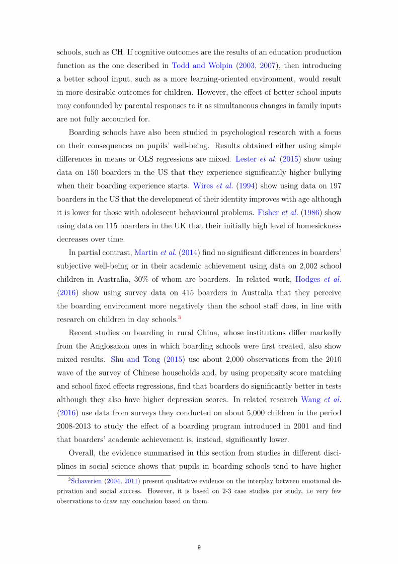
Boarding schools have also been studied in psychological research with a focuson their consequences on pupils’ well-being. Results obtained either using simpledifferences in means or OLS regressions are mixed. Lester et al. (2015) show usingdata on 150 boarders in the US that they experience significantly higher bullyingwhen their boarding experience starts. Wires et al. (1994) show using data on 197boarders in the US that the development of their identity improves with age althoughit is lower for those with adolescent behavioural problems. Fisher et al. (1986) showusing data on 115 boarders in the UK that their initially high level of homesicknessdecreases over time.

In partial contrast, Martin et al. (2014) find no significant differences in boarders’subjective well-being or in their academic achievement using data on 2,002 schoolchildren in Australia, 30% of whom are boarders. In related work, Hodges et al.(2016) show using survey data on 415 boarders in Australia that they perceivethe boarding environment more negatively than the school staff does, in line withresearch on children in day schools.3

Recent studies on boarding in rural China, whose institutions differ markedlyfrom the Anglosaxon ones in which boarding schools were first created, also showmixed results. Shu and Tong (2015) use about 2,000 observations from the 2010wave of the survey of Chinese households and, by using propensity score matchingand school fixed effects regressions, find that boarders do significantly better in testsalthough they also have higher depression scores. In related research Wang et al.(2016) use data from surveys they conducted on about 5,000 children in the period2008-2013 to study the effect of a boarding program introduced in 2001 and findthat boarders’ academic achievement is, instead, significantly lower.

Overall, the evidence summarised in this section from studies in different disci-plines in social science shows that pupils in boarding schools tend to have higher

3Schaverien (2004, 2011) present qualitative evidence on the interplay between emotional de-privation and social success. However, it is based on 2-3 case studies per study, i.e very fewobservations to draw any conclusion based on them.

69

achievement and that this seems to be driven by higher motivation and study ef-fort. Although this evidence expands our knowledge on the role played by boardingschools, to the best of our knowledge no study has tested whether a conducive board-ing environment can compensate, through substitution of family and school inputs,for high ability children with a low SES.

3 Institutions and data

In this section we describe the institutional setting of compulsory education in Eng-land, along with the main characteristics of CH, grammar and independent schoolsin section 3.1. We then describe the data we use in the empirical analysis in section3.2.

3.1 Institutional setting

The state school system in England entails 11 years of compulsory education dividedinto two phases, primary and secondary, and 4 Key Stages, summarised in Table1. Primary school starts with Key Stage 1 (age 5 to 7) and it is followed by KeyStage 2 (age 7-11), whereas secondary school starts with Key Stage 3 (age 11 to 14)followed by Key Stage 4 (age 15-16). All Key Stages end with a national standardisedassessment, either carried out by teachers or externally and the Department forEducation set a level or target that pupils are expected to achieve in compulsorytests in English, Math and Science. Pupils’ tests are marked using an integer scorefrom 0 to 100. Targets are cutoff values in test scores that are set out to help pupils,parents and schools interpreting progress throughout compulsory education.

Table 1: Compulsory education in EnglandPhase Age School Key Assessment Expected

year Stage achievement level5-7 1-2 1 Teachers 2

Primary (state schools)School 7-11 3-6 2 External 4

(state schools)11-14 7-9 3 Teachers 5 or 6

Secondary (state schools)School 15-16 10-11 4 External (GCSE) 5 GCSEs

(all schools) at A*-C

CH is an independent selective and boarding-only mixed school that funds over

710

80% of the costs of pupils’ education. It is a Christian institution dedicated toproviding every year a stable background and boarding education of high standardto 830 boys and girls, having regard especially to children of those families in social,financial or other particular need, as stated in its mission statement. It is located inWest Sussex, in South-East England, and anecdotal evidence suggests that it reliesmainly on word of mouth by its alumni for publicity.

Applicants to CH have to meet its academic standards and also be judged suitableto board. They are expected to be working towards level 5 at Key Stage 2 inEnglish, Maths and Science. After a first selection based on school reports, successfulapplicants are invited in for an initial assessment in English and Maths. Those whopass it will be asked in for a second assessment stage consisting in additional Englishand Maths tests a few months later and also to stay in the school overnight: thiswill help the school to assess their suitability to board. Calculations from CH showthat each assessment stage screens approximately 50% of all applicants. Overall,achievement at Key Stage 2, SES and suitability to board are CH admission criteria.

Mixed grammar schools, our first control group, are highly selective, academically-oriented for historical reasons and include different school types. In our data, about38% of pupils are in Academy Converters grammars, that are independent of controlfrom local authorities, 28% are Foundation and 17% are Voluntary Aided or Volun-tary Controlled, that also enjoy some degree of independence from local authoritiesalthough a lower one relative to Academies. The remaining 13% are Communitygrammars, that are not independent of control from local authorities.

Our second control group are independent schools, which are fee-paying privateschools that are attended by about 7% of pupils either as day pupils or as boarders.The schools for pupils up to ages 11 or 13 are typically referred to as preparatoryschools and from age 11 or 13 they can attend senior or high school. Some indepen-dent schools cover the full age range from age 3 to 18. Since CH is Christian, werestrict our attention to Christian independent day schools to study the boardingeffect. Independent schools set their own examinations at the end of each year andthe only national assessment their pupils sit during compulsory schooling is GCSE.4

4The percentage of pupils attending independent schools varies between about 5% for pupilsaged 5-10, 8% for those aged 11 to 15, and 18% for those aged 16 to 18. About 13.5% of pupilsare boarders in independent schools and only 1% of all independent schools has only boardingpupils. The average termly boarding fee is 8,780 pounds while the average termly day fee is 3,903pounds. Bursaries, scholarships and discounts are available: around 8% of pupils have receivedmeans-tested bursaries and 1% of all pupils paid no fees at all (Independent Schools Council, 2014).

811

Table 2: Resources in different types of schoolsCH Grammar Independent State

Pupil/teacher ratio 8.800 16.444 7.911 14.652Full-time qualified teachers per-pupil 0.101 0.053 0.147 0.072Part-time qualified teacher per-pupil 0.020 0.016 0.119 0.026Total n. qualified teachers per-pupil 0.121 0.069 0.266 0.099

Grammar schools are funded by the government as they are state schools. In-dependent schools, instead, currently receive no direct government funding, thoughabout 80% of them are constituted as charities (Independent Schools Council, 2014)and therefore receive important tax exemptions. They receive most of their incomein the form of fees. Table 2 shows proxies of schools’ teaching resources separately forCH, for our control groups and for state schools. To quantify potential differences,we matched pupil-level data on achievement and school-type to school-level dataprovided by the Department for Education (School Workforce Census for the schoolyear 2006/07) with information on schools’ resources, using the school identifier tomatch them. The teaching resources of CH are quite close to those of independentschools. Relative to grammars, however, CH has a substantially lower pupil/teacherratio and a higher number of qualified teachers per pupil. Relative to other stateschools, both CH and independent schools have higher resources while grammarshave similar ones to other state schools. Finally, independent schools also devotevery substantially more than state schools to non-teaching resources which may havespillover benefits for academic outcomes (Davies and Davies, 2014).

3.2 Data

Our analysis is based on individual-level administrative data on England, the Na-tional Pupil Database (NPD) matched with the Pupil Level Annual School Census,that contain information on attainment and a set of pupil characteristics for allthose enrolled in state schools since primary education. The final dataset, withabout 2 million pupils, contains information on five cohorts who attended primarystate schools and sat their Key Stage 2 tests in years 2002-2006 and accordingly satGCSEs at the end of Key Stage 4 in years 2007-2011.

Out of all pupils in the data, 429 went to CH after completing primary educationin state schools, or about 86 pupils on average each year. About 70,000 went tosecondary grammar schools and about 80,000 to independent ones. These pupilsare our control groups and, in the remaining of this section, we will describe in

912

detail the criteria to select the subsample that we will use in the empirical analysis.5

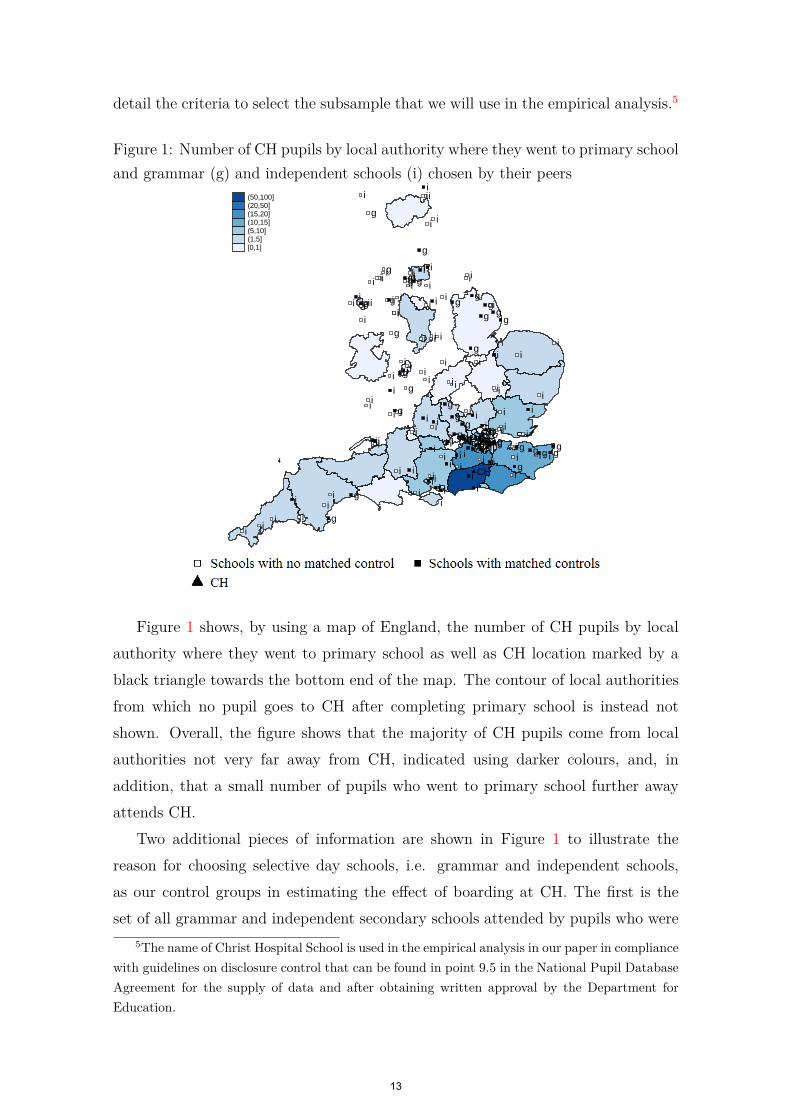
Figure 1: Number of CH pupils by local authority where they went to primary schooland grammar (g) and independent schools (i) chosen by their peers

g

g

g

g

gg

ggg

g

g

g

g

gg

gg

g gg

g

g

g

gg

g

g

g

g

CH

gggggg

g

g

g

g

i

ii i

ii i ii

i i

iiiiii

i

ii

i

i

i

i i

iiii

ii

i

i

i

ii

i

i i

i iii

i

ii

iii

i

ii ii

ii

iii

i

i

ii i

i

i

ii

ii

i

i ii

ii

i

ii i

ii

i

i

i i

ii

i

i

iii

i

i

ii

ii

i i

iii i

ii

i

iii

i

iiiii

ii

iiii

i

i

ii

i i

ii

i

i

i

(50,100](20,50](15,20](10,15](5,10](1,5][0,1]

Figure 1 shows, by using a map of England, the number of CH pupils by localauthority where they went to primary school as well as CH location marked by ablack triangle towards the bottom end of the map. The contour of local authoritiesfrom which no pupil goes to CH after completing primary school is instead notshown. Overall, the figure shows that the majority of CH pupils come from localauthorities not very far away from CH, indicated using darker colours, and, inaddition, that a small number of pupils who went to primary school further awayattends CH.

Two additional pieces of information are shown in Figure 1 to illustrate thereason for choosing selective day schools, i.e. grammar and independent schools,as our control groups in estimating the effect of boarding at CH. The first is theset of all grammar and independent secondary schools attended by pupils who were

5The name of Christ Hospital School is used in the empirical analysis in our paper in compliancewith guidelines on disclosure control that can be found in point 9.5 in the National Pupil DatabaseAgreement for the supply of data and after obtaining written approval by the Department forEducation.

1013

in a primary school located in the same local authority as those attended by CHpupils, marked using squares and with ‘g’ and ‘i’ respectively in the figure. The factthat these schools are located either in the same local authority or in adjacent onesshows that pupils may not choose the closest secondary school in the local authorityin which they attended primary school. The second and related information is theset of schools actually chosen by pupils similar to those at CH, i.e. matched usingthe propensity score that will be defined in section 4. They are marked as blacksquares while white square indicate schools attended by pupils not similar enoughto CH ones, according to the propensity score, and show heterogeneity in pupils’characteristics even between selective day schools.

Pupils who attended grammar secondary schools are the first control group thatwe use to obtain an estimate of the effect of attending CH as, like CH, are aca-demically selective while they differ through not offering boarding and through hav-ing substantially fewer resources. The second control group consists of pupils whoattended independent Christian day schools after state primary as, like CH, areacademically selective to varying degrees and deploy far more resources than stateschools (Green et al., 2012). Like CH, 90% of independent schools in our datahave a Christian foundation, either Church of England or Roman Catholic, and theremaining are not religious.

In addition, we restrict our analysis to pupils in grammar and in independentschools who went to a primary school in the same local authorities as those attendedby pupils at CH, who are approximately 10% of all pupils in grammar and in inde-pendent schools. This restriction ensures that CH pupils and those in the controlgroup face the same choice set of secondary schools and, in addition, they live inthe same geographical area and are ruled by the same local government.

Figure 2 shows scatterplots of the percentage of pupils on FSM, measured onthe vertical axis, and the percentage of pupils that obtained the top level in KeyStage 2 tests, i.e. 5, in all three subjects, measured on the horizontal axis, by usingschool-level data. CH is marked in the figure using a black triangle while the blacksquares show the grammar and independent schools chosen by pupils who are verysimilar to those at CH, i.e. matched using the propensity score.

The grammar and independent schools shown in Figure 2 have been selected assome of their pupils are very similar, i.e. matched, to those at CH and we also noticethat a high percentage of their pupils obtains level 5 in all Key Stage 2, particularlyfor grammar schools. However, CH stands out with a percentage of admitted pupils

1114

Figure 2: Achievement at Key Stage 2 (KS2) and % FSM by secondary school

CH

0

.05

.1

.15%

chi

ldre

n on

FS

M

.5 .6 .7 .8 .9 1% lev. 5 KS2 Eng., Mat. & Sci.

CH and grammarCH

0

.05

.1

.15

0 .2 .4 .6 .8 1% lev. 5 KS2 Eng., Mat. & Sci.

CH and independent

Schools with matched controls CH

on FSM twice or three times higher than in the grammar and independent schoolsshown in the figure.6

Figure 3 shows histograms of achievement at Key Stage 1, 2 and 4 using our fulldataset with 2 million pupils to help us defining meaningful achievement measuresfor the pupils in selective schools in our empirical analysis. The central panel showsthat the percentage obtaining in individual tests a level greater than 4, that pupilsare expected to achieve and coincides with the modal frequency, varies between 30and 40%. The percentage obtaining 5 in all tests, that was used in Figure 2 asa measure of high achievement at Key Stage 2 is, instead, typically lower. Figure3 also shows in the top panel histograms of achievement levels at Key Stage 1, inwhich the expected level is 2 and it coincides with the modal frequency. Hence,in the empirical analysis we will use as predetermined measures of achievement adummy equal to 1 if a pupil obtains a level greater than 2 by subject at Key Stage1 and a dummy equal to 1 if a level greater than 4 by subject is obtained at KeyStage 2, in addition to using Key Stage 2 tests scores.

We chose three binary variables, i.e. dummies, as outcomes. The first one is equalto 1 if a pupil obtains at least one GCSE at A and 0 otherwise. The histogram onthe left-hand side in the bottom panel in Figure 3 shows that only pupils who areapproximately in the top quartile of the distribution of the number of GCSEs at

6Additional information about how pupils are matched is found in section 4.

1215

Figure 3: Histograms of achievement at Key Stage 1 and 2 and at GCSE

0

.2

.4

.6

Den

sity

0 1 2 3 4

Key Stage 1 Engl. level

0

.2

.4

.6

Den

sity

0 1 2 3 4

Key Stage 1 Maths level

0

.2

.4

.6

.8

Den

sity

0 1 2 3 4

Key Stage 1 Science level

0

.1

.2

.3

.4

.5

Den

sity

2 3 4 5 6

Key Stage 2 Engl. level

0

.1

.2

.3

.4

.5

Den

sity

2 3 4 5 6

Key Stage 2 Maths level

0

.1

.2

.3

.4

.5

Den

sity

2 3 4 5 6

Key Stage 2 Science level

0

.2

.4

.6

Den

sity

0 5 10 15

N. of GCSE with A

0

.2

.4

.6

.8

Den

sity

0 5 10 15

N. of GCSEs with A*

0

.2

.4

.6

Den

sity

0 5 10 15

N. of GCSEs with A-A*

A obtain this qualification. The second one is equal to 1 if at least one GCSE isat A* and 0 otherwise, with only 10-15% of pupils obtaining this qualification, asshown by the histogram of the number of GCSEs at A* in the centre in the bottompanel in Figure 3. Finally, the third one is equal to 1 if 5 or more GCSEs are at Aor A*, with only pupils in the top decile achieving this, as shown by the histogramof the number of GCSEs at A-A* on the right-hand side in the bottom panel inFigure 3. These outcomes are typically good predictors of the decision to enrol inpost-compulsory education (Chowdry et al., 2013).7

We try to match pupils at CH with as similar as possible ones in grammar or inde-pendent schools according to additional predetermined characteristics. They includesocio-demographics, such as gender, ethnicity, quarter of birth and two proxies forSES. The first is the income deprivation affecting children index (IDACI), measuringthe share of children in low income households in an area of about 40 households

7In choosing our outcomes of interest we focused on the highest grades in GCSEs, i.e. A orA*, since all secondary schools we consider are selective and its pupils tend to achieve towardsthe high end of the distribution of grades in GCSEs. We did not choose, instead, the probabilityof achieving five or more GCSEs at A*-C, a lower grade, as it is about 98% in selective schoolsand, similarly, the mean number of GCSEs taken by pupils in these schools is 10 and shows littlevariation across schools. Achievement in English and Maths at GCSE are not used as outcomesas this information is not available for CH and for independent schools in NPD data.

1316

and 100 persons called super output areas, that is the smallest unit used for censuspurposes. The second is a dummy equal to 1 if a pupil obtains a Free School Meal(FSM) as her/his parents receive some form of income support. Extra dummies areused to measure if a pupil takes English as an additional language (EAL) where it isnot his/her native language and whether a pupil has special education needs (SEN),both being assessed case-by-case by educational specialists in schools.

A preview of the descriptive statistics of pupils’ relevant predetermined charac-teristics, that are shown in Figure 5 in section 4 separately for pupils at CH and incontrol schools shows that differences are small and not significant.

4 Econometric strategy

We estimate the effect of going to CH on achievement in the compulsory schoolleaving exams and whether it differs by SES and gender using propensity score(pscore) matching, an econometric strategy based on selection on observables. Thisis possible thanks to the unique admission criteria based jointly on merit and onSES and to the rich set of pupils’ observable characteristics in the administrativedata.

∆AT T = E[A(1)− A(0) | D = 1] (1)

Let D be a dummy indicating whether pupils go to CH, with D = 1 for pupilsat CH (treatment) and D = 0 for those in a selective day school (controls). Letalso A(1) and A(0) be the potential outcome, i.e. achievement, for treated andfor controls. Finally, let X be a set of predetermined observable characteristics forpupils. Our parameter of interest is the average treatment on the treated (ATT),which we denote ∆AT T and define in our setting as the mean effect of attending CH,i.e. the treatment group, rather than a selective day school, i.e. the control group,as shown in equation (1).

To recover via the law of iterated expectations the unobservable term E[E[A(0) |D = 0] | D = 1] in equation (1) we rely on the assumption that admission to CHdepends only on unobservables, also known as selection on observables or Condi-tional Independence Assumption (CIA). Under this assumption assignment to thetreatment or to the control group is independent on the treatment D conditional onthe set of observables X, formally A(1), A(0) ⊥ D | X. However, when the number

1417

of observable characteristics in the vector X is high, it may not be possible to findfor some pupils at CH pupils in control schools with the same observables X, unlessthe number of observations in the data is very high. This problem, known as curseof dimensionality, is solved by using instead the probability of going to CH givenobservable characteristics X or pscore, i.e. P (D = 1 | X).

In addition, we ensure that for each pupil at CH there is one or more with verysimilar observables in the control group by imposing the common support (CS)condition, i.e. 0 < P (D = 1 | X) < 1. Finally, after estimating the pscore with alogit model, we match treated pupils with very similar pupils from the control groupby using nearest neighbour matching method. By using as two different controlgroups grammar and independent schools, we obtain two sets of estimates. While inour preferred specification we use the nearest neighbour method to match pupils, wealso assess the sensitivity of our results to using different matching methods basedon the pscore.8

In our analysis so far, the assumption we made was that the choice faced by tal-ented pupils was binary: either CH or another type of selective school, for examplean independent school. However, at the end of primary school a talented pupil mayhave been granted admission to CH, as well as to a grammar and an independentsecondary school. This can be accounted for by extending the binary propensityscore matching framework to the case of multiple treatments thanks to the match-ing estimator proposed in Lechner (2002). By allowing multiple treatments, thetreatment variable D in our setup is no longer binary and can, instead, take multi-ple values. In our setup of secondary school choice, D is equal to 0 if a pupil choosesan independent school, which we set as the baseline although this choice does notaffect results, to 1 if the choice is a grammar one and to 2 for CH.

Firstly, a multinomial logit model of school choice is estimated using as covari-ates the set of observables X. Secondly, we compute the predicted probabilitiesP̂ j(X) = P̂ (D = j | X) of attending an independent school (j = 0), a gram-mar school (j = 1) or CH (j = 2). To estimate the effect of attending CH rela-tive to, for example, an independent school we compute the conditional probabilityP̂ 2|2,0(X) = P̂ 2(X)

P̂ 2(X)+P̂ 0(X) . Finally, the estimated conditional probability is used inLechner (2002) as balancing score in a matching estimator setting with multipletreatments to estimate the unobserved term E[E[A(0) | D = 0, P 2|2,0] | D = 2], i.e.

8ATT estimation with binary treatment was conducted using the software routines describedin Becker and Ichino (2002); Leuven and Sianesi (2015).

1518

to match pupils at CH (D = 2) and pupils in independent schools (D = 0) withvery similar values of the conditional probability P 2|2,0. Analogously, the procedureis repeated to estimate the effect of attending CH relative to a grammar school.9

5 Results

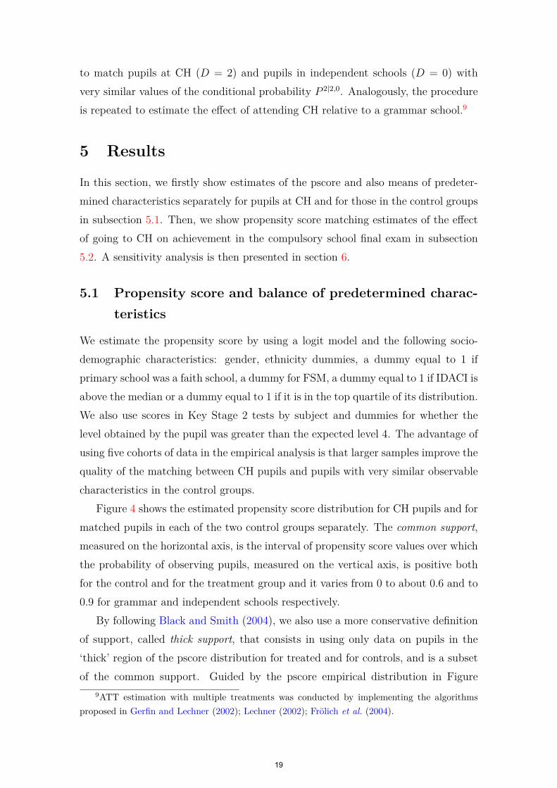
In this section, we firstly show estimates of the pscore and also means of predeter-mined characteristics separately for pupils at CH and for those in the control groupsin subsection 5.1. Then, we show propensity score matching estimates of the effectof going to CH on achievement in the compulsory school final exam in subsection5.2. A sensitivity analysis is then presented in section 6.

5.1 Propensity score and balance of predetermined charac-teristics

We estimate the propensity score by using a logit model and the following socio-demographic characteristics: gender, ethnicity dummies, a dummy equal to 1 ifprimary school was a faith school, a dummy for FSM, a dummy equal to 1 if IDACI isabove the median or a dummy equal to 1 if it is in the top quartile of its distribution.We also use scores in Key Stage 2 tests by subject and dummies for whether thelevel obtained by the pupil was greater than the expected level 4. The advantage ofusing five cohorts of data in the empirical analysis is that larger samples improve thequality of the matching between CH pupils and pupils with very similar observablecharacteristics in the control groups.

Figure 4 shows the estimated propensity score distribution for CH pupils and formatched pupils in each of the two control groups separately. The common support,measured on the horizontal axis, is the interval of propensity score values over whichthe probability of observing pupils, measured on the vertical axis, is positive bothfor the control and for the treatment group and it varies from 0 to about 0.6 and to0.9 for grammar and independent schools respectively.

By following Black and Smith (2004), we also use a more conservative definitionof support, called thick support, that consists in using only data on pupils in the‘thick’ region of the pscore distribution for treated and for controls, and is a subsetof the common support. Guided by the pscore empirical distribution in Figure

9ATT estimation with multiple treatments was conducted by implementing the algorithmsproposed in Gerfin and Lechner (2002); Lechner (2002); Frölich et al. (2004).

1619

Figure 4: Kernel density estimate of the propensity score

0

5

10

15F

requ

ency

(%

)

0 .2 .4 .6 .8Estimated pscore

CH (---) vs Independent

0

2

4

6

8

Fre

quen

cy (

%)

0 .2 .4 .6 .8 1Estimated pscore

CH (---) vs Grammar

4, we chose as thick support the interval between 0 and 0.2 and an even smallerinterval, 0-0.1, i.e. we drop observations for pupils with pscore in the right tail ofthe distribution. Estimates obtained after excluding pupils outside the thick supportregion are helpful to assess whether those obtained under the common support arepotentially biased due to self-selection into or out of CH, since it is more likely forpupils in the tails rather than in the middle of the pscore distribution.

Descriptive statistics of pupils’ predetermined characteristics by the time theystarted secondary education, that are used to assess the balancing property afterestimating the propensity score, are shown in Figure 5. The vertical axis on the left-hand side measures the difference between pupils at CH and controls in, for example,the relative frequency of females in the top left of the figure, separately for pscoreblocks measured along the horizontal axis. After estimating the pscore, the blockswere defined along the pscore support to ensure that predetermined characteristicsare balanced. Pscore estimation using pupils in grammar schools as controls requiredsplitting the data sample into 7 different blocks according to pupils’ estimated pscorewhile 9 blocks were used when the control group were pupils in independent schools.In addition, the vertical axis on the right-hand side measures p-values of t-tests ofthe null hypothesis of no difference in the mean value between treated and controlsby block.

1720

Figure 5: Covariates differences for CH relative to grammar and independent bypscore block

0.2.4.6.81

P-v

alue

-.2

0

.2

.4

Cov

. diff

.

1 2 3 4 5 6 7 8 9

Female

0.2.4.6.81

P-v

alue

-.2

-.1

0

.1

.2

Cov

. diff

.

1 2 3 4 5 6 7 8 9

White

.2

.4

.6

.8

1

P-v

alue

-.06-.04-.02

0.02.04

Cov

. diff

.

1 2 3 4 5 6 7 8 9

Asian

0

.2

.4

.6

.8

P-v

alue

-.1

0

.1

.2

.3

Cov

. diff

.

1 2 3 4 5 6 7 8 9

KS2 Faith school

0.2.4.6.81

P-v

alue

-202468

Cov

. diff

.

1 2 3 4 5 6 7 8 9

KS2 English score

0.2.4.6.81

P-v

alue

-5

0

5

10C

ov. d

iff.

1 2 3 4 5 6 7 8 9

KS2 Math score

0

.2

.4

.6

.8

P-v

alue

-101234

Cov

. diff

.

1 2 3 4 5 6 7 8 9

KS2 Science score

0.2.4.6.81

P-v

alue

-.05

0

.05

.1

.15

Cov

. diff

.

1 2 3 4 5 6 7 8 9

KS2 English > 4

0.2.4.6.81

P-v

alue

-.2

-.1

0

.1

.2

Cov

. diff

.

1 2 3 4 5 6 7 8 9

KS2 Math > 4

.2

.4

.6

.8

1P

-val

ue

-.05

0

.05

.1

Cov

. diff

.

1 2 3 4 5 6 7 8 9

KS2 Science > 4

0

.2

.4

.6

.8

P-v

alue

-.04

-.02

0

.02

.04

Cov

. diff

.

1 2 3 4 5 6 7 8 9

IDACI > median

.2

.4

.6

.8

1

P-v

alue

-.04

-.02

0

.02

Cov

. diff

.

1 2 3 4 5 6 7 8 9

IDACI top quartile

0.2.4.6.8

P-v

alue

-.2-.15

-.1-.05

0.05

Cov

. diff

.

1 2 3 4 5 6 7 8 9Pscore block number

IDACI

.2

.4

.6

.81

P-v

alue

-.05

0

.05

.1

Cov

. diff

.

1 2 3 4 5 6 7 8 9Pscore block number

FSM

Diff. gram. Diff. indep.P-value gram. P-value indep.

1821

The plot on the top left in Figure 5 shows that the difference in the relativefrequency of females by pscore block in CH relative to grammar schools, reportedusing a continuous line marked by diamonds, is either slightly positive or zero andp-values, reported using a scatterplot of diamonds, are greater than the 5% con-ventional level. The difference in the frequency of females by pscore block at CHrelative to independent schools is reported, instead, using a dotted line marked bycircles and its p-values, reported using a scatterplot of circles, are also greater than5%. Overall, Figure 5 shows that predetermined characteristics are balanced, exceptfor p-values close to 5% for some pscore blocks of Key Stage 2 scores. This suggeststhat the propensity score was helpful to choose in grammar and in independentschools those pupils who are most similar to pupils at CH in terms of observables.10

5.2 The effect of CH on achievement

In this section, we report ATT estimates of the impact on achievement in the compul-sory school final exam of attending CH, rather than a day grammar or independentschool, to test our first hypothesis that offering a better learning and non-schoolenvironment to high ability pupils with low SES increases their achievement (H1).Overall, the positive and significant ATT estimates in Table 3 offer support to ourhypothesis.

Table 3: Effect of attending CH on results in school-leaving examsGrammar schools Independent schools

ATT Matched All ATT Matched All1+ GCSE with A 0.044∗∗ 0.888 0.868 0.100∗∗∗ 0.832 0.754S.e. 0.020 0.0241+ GCSE with A* 0.170∗∗∗ 0.653 0.570 0.084∗∗ 0.739 0.527S.e. 0.031 0.0315+ GCSE with A-A* 0.174∗∗∗ 0.593 0.513 0.126∗∗∗ 0.641 0.422S.e. 0.033 0.034N 494 7,075 369 8,118∗ p < 0.10, ∗∗ p < 0.05, ∗∗∗ p < 0.01

To match controls to treated we used as our preferred method nearest neighbourmatching with replacement and set to 0.01 the maximum distance in pscore that is

10Since in Figure 5 the difference in the relative frequency of pupils with an IDACI above themedian or an IDACI in the top quartile is zero in some blocks, corresponding p-values are notreported.

1922

allowed to perform a match. The estimates in Table 3, obtained using the commonsupport, show that the probability of obtaining at least 1 (1+ hereafter) GCSEswith A is 4.4 and 10 percentage points (ppt hereafter) higher relative to grammarand independent schools respectively, with ATT estimates being significant. This is5% and 12% higher relative to the value for matched controls, that is also shown inthe table. Differences in the probability of obtaining 1+ GCSEs with A* are alsosignificant and show that the point estimate is 17 and 8.4 ppt higher or about 26%and 11% relative to grammar and independent schools. Finally, the probability ofobtaining 5+ GCSEs with A-A* is 17.4 and 12.6 ppt higher or about 29% and 20%relative to the control groups respectively. Overall, the point estimates are higherwhen using as outcome the dummy equal to 1 if pupils obtain 1+ GCSEs with A* or5+ GCSEs with A-A*, who are approximately in the top decile of the distribution ofachievement in GCSE exams among all pupils in the administrative data, as shownin Figure 3.11

In addition to ATT estimates and mean values of outcomes for matched controls,Table 3 also shows mean values for all controls to compare our ATT estimateswith naive estimates obtained as the difference in mean achievement between CHpupils and all pupils in grammar and in independent schools respectively. Naiveestimates have the same sign as our ATT estimates. However, the point estimatesare greater since the mean value of the outcomes for all controls is smaller thanfor matched controls. Under our untestable identifying assumption of selection onobservables naive estimates are then biased upwards relative to our ATT estimates.This comparison also suggests that had pupils at CH instead gone to grammar orindependent day schools, they would have obtained higher scores than the averagein those schools.

Finally, Table 3 shows that the ATT for the probability of obtaining 1+ GCSEsat A, i.e. of being a moderately high achiever at GCSE, is higher at CH whencontrols are pupils from independent schools while the probability of obtaining 1+GCSEs at A* or 5+ GCSEs at A-A*, i.e. of being a very high achiever, tends tobe higher when controls are from grammar schools. However, the significance of

11Results not reported but available upon request show that ATT estimates change little ifadditional predetermined characteristics are used, such as achievement in all tests at Key Stage1, the type of school at Key Stage 2 and the distance to the closest secondary schools. However,since we used as criterion to choose the predetermined characteristics that are used as covariatesin estimating the pscore the results of covariates balancing analysis that is described in section 5.1,we did not use these additional covariates as they were slightly unbalanced.

2023

the difference is not testable with our econometric strategy based on selection onobservables without making additional assumptions.

Table 4: Effect of attending CH for pupils in the pscore thick supportGrammar schools Independent schools

ATT Matched All ATT Matched AllPscore thick support 0-0.2

1+ GCSE with A 0.065∗∗∗ 0.868 0.868 0.072∗∗∗ 0.856 0.754S.e 0.021 0.0261+ GCSE with A* 0.192∗∗∗ 0.623 0.570 0.084∗∗ 0.730 0.527S.e 0.032 0.0345+ GCSE with A-A* 0.179∗∗∗ 0.576 0.513 0.126∗∗ 0.631 0.422S.e 0.034 0.037N 450 7,075 306 8,118

Pscore thick support 0-0.11+ GCSE with A 0.079∗∗∗ 0.844 0.868 0.081∗∗∗ 0.856 0.754S.e 0.026 0.0301+ GCSE with A* 0.231∗∗∗ 0.576 0.570 0.077∗ 0.703 0.527S.e 0.038 0.0435+ GCSE with A-A* 0.218∗∗∗ 0.523 0.513 0.126∗∗∗ 0.581 0.422S.e 0.040 0.046S.e 338 7,075 214 8,118∗ p < 0.10, ∗∗ p < 0.05, ∗∗∗ p < 0.01

Table 4 reports additional ATT estimates of the impact of attending CH relativeto control schools for pupils whose pscore is in a ‘thick’ region of the pscore distri-bution, following Black and Smith (2004). We define as thick support pscore valuesin the range 0-0.2 and, additionally, a more narrow range: 0-0.1. Table 4 showsoverall that our main results are robust to using only pupils in the thick supportwhen considering the sign of the point estimates, as well as their size and signif-icance. However, slight differences emerge across control groups. Thick supportestimates when pupils in grammar schools are the controls are slightly greater thanthose obtained on the common support, with the greatest differences being for theprobability of obtaining 1+ GCSEs at A. When looking, instead, at thick supportestimates obtained with pupils in independent schools as controls, Table 4 showsthat they are very similar to common support ones.12

ATT estimates for subsamples of pupils by gender and by SES are shown in12In choosing the pscore intervals defining the thick support regions, we use as guidance the

empirical distribution of pscores in Figure 4.

2124

Table 5: Effect of attending CH for pupils’ subgroups by gender and SESGrammar schools Independent schools

ATT Matched All ATT Matched AllMales

1+ GCSE with A 0.081∗∗∗ 0.856 0.848 0.127∗∗∗ 0.810 0.722S.e. 0.028 0.0341+ GCSE with A* 0.177∗∗∗ 0.587 0.527 0.072∗ 0.692 0.495S.e. 0.044 0.0445+ GCSE with A-A* 0.127∗∗∗ 0.560 0.471 0.093∗∗ 0.595 0.390S.e. 0.046 0.047N 292 3,701 208 5,460

Females1+ GCSE with A -0.016∗∗∗ 0.944 0.890 0.151∗∗∗ 0.776 0.746S.e. 0.026 0.0381+ GCSE with A* 0.174∗∗∗ 0.722 0.618 0.214∗∗∗ 0.682 0.518S.e. 0.041 0.0445+ GCSE with A-A* 0.190∗∗∗ 0.675 0.558 0.271∗∗∗ 0.594 0.423S.e. 0.044 0.047N 227 3,374 169 3,230

IDACI below median1+ GCSE with A 0.002 0.930 0.881 0.117∗∗∗ 0.818 0.782S.e. 0.028 0.0421+ GCSE with A* 0.124∗∗∗ 0.652 0.607 0.080 0.693 0.550S.e. 0.049 0.0565+ GCSE with A-A* 0.152∗∗∗ 0.575 0.544 0.102∗ 0.620 0.451S.e. 0.052 0.059N 227 3,562 126 4,393

IDACI above median1+ GCSE with A 0.055∗∗ 0.877 0.854 0.089∗∗∗ 0.842 0.679S.e. 0.026 0.0311+ GCSE with A* 0.172∗∗∗ 0.679 0.534 0.113∗∗∗ 0.733 0.456S.e. 0.041 0.0395+ GCSE with A-A* 0.190∗∗∗ 0.601 0.481 0.147∗∗∗ 0.640 0.352S.e. 0.044 0.043N 274 3,513 227 4,297

FSM1+ GCSE with A 0.174∗∗ 0.754 0.777 0.130∗ 0.797 0.335S.e. 0.080 0.0731+ GCSE with A* 0.275∗∗∗ 0.551 0.458 0.203∗∗ 0.623 0.196S.e. 0.103 0.0965+ GCSE with A-A* 0.290∗∗∗ 0.449 0.343 0.159 0.580 0.149S.e. 0.105 0.100N 44 251 43 409

No FSM1+ GCSE with A 0.050∗∗ 0.884 0.871 0.089∗∗∗ 0.844 0.751S.e. 0.021 0.0251+ GCSE with A* 0.174∗∗∗ 0.648 0.575 0.097∗∗∗ 0.725 0.519S.e. 0.032 0.0335+ GCSE with A-A* 0.183∗∗∗ 0.589 0.519 0.167∗∗ 0.606 0.415S.e. 0.034 0.036N 437 6,824 328 8,281∗ p < 0.10, ∗∗ p < 0.05, ∗∗∗ p < 0.01

2225

Table 5. Results separately by gender are in line with common support estimatesexcept the very small and negative effect of obtaining 1+ GCSE at A for females,suggesting some heterogeneity by gender for those pupils who are not among topachievers at CH since the result for males is positive. Heterogeneity by gender alsoseems to be present among top achievers, i.e. pupils with 5+ GCSE at A-A*, as itis shown by greater point estimates for females.

We examined subsamples by SES in two alternative ways. First, we obtainedestimates for pupils who live in an area with an IDACI value above the median ofthe distribution, i.e. poor areas, and contrast these with estimates for those withan IDACI value below the median, i.e. a more affluent areas. Second, we comparedestimates for pupils according to whether or not they were on FSM. When we lookat results separately by whether IDACI is low or high, we find that achievementgains arising from attending CH tend to be higher for pupils with a high IDACI.Results by FSM are similar although when the controls are pupils in grammarstheir precision is lower due to the low number of matched controls. However, wecannot fully test these differences in a selection on observables framework withoutadditional assumptions.

To summarise, ATT point estimates of the effect of attending CH are greaterwhen using as outcomes proxies for high achievers at GCSE, i.e. 1+ GCSEs atA* or 5+ GCSEs with A-A*, who are among the top 10-15% in the distribution ofachievement at GCSE. For these same variables, estimates of the CH effect obtainedusing grammar school pupils as controls tend to be greater than those obtained usingindependent school pupils. When we consider only those pupils in the thick supportregion, we find that point estimates are very similar to those obtained using thecommon support. This similarity suggests that estimates are driven by pupils in themiddle of the achievement distribution at GSCE rather than by those in the tailstail and hence that they are little confounded by self-selection in the right tail of thepropensity score distribution. Finally, we find that the effect is greater and tends tobe more precise for females and for children in poor households.

6 Sensitivity analysis

In this section we perform a sensitivity analysis of our main results. Firstly, we com-pare them with matching estimates obtained by allowing for multiple treatments, i.e.CH, grammar or independent schools, rather than a binary one, following Lechner

2326

(2002). Table 6 shows matching estimates that were obtained by letting the dif-ferent types of selective schools that we consider be multiple treatments. The signand size of the two sets of point estimates, as well as their significance, are in linewith our main results in Table 3, that are obtained by assuming, instead, a binarytreatment. Overall, this suggests that relaxing the assumption of modelling choiceof CH relative to a different selective secondary school as a binary treatment doesnot substantially alter our main results. The only difference is that the estimateof the probability of obtaining 1+ GCSE at A with pupils in grammar schools ascontrols is smaller and no longer significant. This may be due to the lower numberof matched controls in grammar schools and may lead to a poorer match relativeto our main results, particularly when looking at the probability of obtaining 1+GCSE at A, as grammar school pupils tend to be very high ability pupils achievingtop grades at Key Stage 2 and at GCSE.

Table 6: Matching estimates of CH effect using pscore from multinomial logit

Grammar schools Independent schoolsATT Mean for controls ATT Mean for controls

Matched All Matched All1+ GCSE with A 0.023 0.907 0.868 0.096∗∗∗ 0.837 0.754S.e. 0.032 0.0241+ GCSE with A* 0.202∗∗∗ 0.622 0.570 0.147∗∗∗ 0.676 0.527S.e. 0.049 0.0325+ GCSE with A-A* 0.183∗∗∗ 0.574 0.513 0.184∗∗∗ 0.583 0.422S.e. 0.051 0.034N 175 7,075 370 8,118∗ p < 0.10, ∗∗ p < 0.05, ∗∗∗ p < 0.01

Secondly, we compare our main results, obtained by using nearest neighbourmatching, with results obtained using different matching methods, as one of thelimitations of nearest neighbour is finding a match for all CH pupils and not con-trolling for the ‘quality’ of the matching, i.e. how similar to pupils at CH are pupilsin control schools in terms of their predetermined characteristics. With kernel andradius matching, instead, a pupil at CH can be matched with more than one pupilin the control group and the estimated counterfactual outcome for that pupil at CHis a weighted average of the outcome value for matched pupils in the control group,with the weight increasing with the quality of the matching. In kernel matching aCH pupil is matched with all pupils in the control group and the weight is inverselyproportional to the distance between the propensity score value for that CH pupil

2427

and for controls.In radius matching, instead, only control group pupils whose value of the propen-

sity score is within a fixed radius from the one of a given CH pupil are matchedwith her/him. The weight is equal to the inverse of the number of matched pupils,which is the same for all controls matched to the same pupil at CH. Finally, insteadof relying on the propensity score as a metric to match treated and controls, we useMahalanobis distance. In the context of matching, this is a scalar measure of thesquare of the distance between the vector of covariates for a pupil at CH relative tothe one for a pupil in the control group, multiplied by the inverse of the covariancematrix of the difference between the vectors.

Table 7: Matching estimates of CH effect using different matching methods

Grammar schools Independent schoolsATT Matched All ATT Matched All

Kernel1+ GCSE with A 0.047∗∗∗ 0.885 0.868 0.129∗∗∗ 0.803 0.754S.e. 0.013 0.0151+ GCSE with A* 0.204∗∗∗ 0.619 0.570 0.165∗∗∗ 0.658 0.527S.e. 0.020 0.0225+ GCSE with A-A* 0.203∗∗∗ 0.564 0.513 0.202∗∗∗ 0.564 0.422S.e. 0.022 0.023N 7,075 8,118

Radius with size 0.11+ GCSE with A 0.056∗∗∗ 0.876 0.868 0.146∗∗∗ 0.787 0.754S.e. 0.013 0.0151+ GCSE with A* 0.230∗∗∗ 0.593 0.570 0.206∗∗∗ 0.617 0.527S.e. 0.019 0.0215+ GCSE with A-A* 0.231∗∗∗ 0.536 0.513 0.244∗∗∗ 0.522 0.422S.e. 0.021 0.023N 7,075 8,118

Mahalanobis1+ GCSE with A 0.049∗∗ 0.883 0.868 0.058∗∗∗ 0.874 0.754S.e. 0.020 0.0221+ GCSE with A* 0.210∗∗∗ 0.613 0.570 0.131∗∗∗ 0.692 0.527S.e. 0.029 0.0285+ GCSE with A-A* 0.203∗∗∗ 0.564 0.513 0.182∗∗∗ 0.585 0.422S.e. 0.028 0.030N 7,075 8,118∗ p < 0.10, ∗∗ p < 0.05, ∗∗∗ p < 0.01

Table 7 shows ATT estimates separately by matching method across differenthorizontal panels. The top panel shows estimates obtained using kernel matching,estimates in the central panel were obtained using radius matching and, finally,

2528

those in the bottom panel using a Mahalonobis distance. Overall, the table showsthat the sign, size and precision of point estimates is in line with our main resultsin Table 3. As for the size of point estimates, those of the probability of obtaining1+ GCSE with A or with A-A* are slightly greater than our main results.13

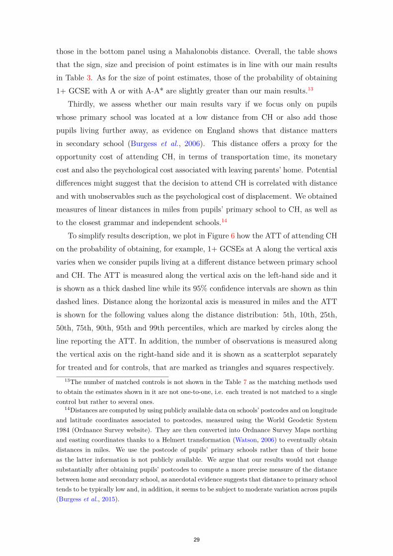
Thirdly, we assess whether our main results vary if we focus only on pupilswhose primary school was located at a low distance from CH or also add thosepupils living further away, as evidence on England shows that distance mattersin secondary school (Burgess et al., 2006). This distance offers a proxy for theopportunity cost of attending CH, in terms of transportation time, its monetarycost and also the psychological cost associated with leaving parents’ home. Potentialdifferences might suggest that the decision to attend CH is correlated with distanceand with unobservables such as the psychological cost of displacement. We obtainedmeasures of linear distances in miles from pupils’ primary school to CH, as well asto the closest grammar and independent schools.14

To simplify results description, we plot in Figure 6 how the ATT of attending CHon the probability of obtaining, for example, 1+ GCSEs at A along the vertical axisvaries when we consider pupils living at a different distance between primary schooland CH. The ATT is measured along the vertical axis on the left-hand side and itis shown as a thick dashed line while its 95% confidence intervals are shown as thindashed lines. Distance along the horizontal axis is measured in miles and the ATTis shown for the following values along the distance distribution: 5th, 10th, 25th,50th, 75th, 90th, 95th and 99th percentiles, which are marked by circles along theline reporting the ATT. In addition, the number of observations is measured alongthe vertical axis on the right-hand side and it is shown as a scatterplot separatelyfor treated and for controls, that are marked as triangles and squares respectively.

13The number of matched controls is not shown in the Table 7 as the matching methods usedto obtain the estimates shown in it are not one-to-one, i.e. each treated is not matched to a singlecontrol but rather to several ones.

14Distances are computed by using publicly available data on schools’ postcodes and on longitudeand latitude coordinates associated to postcodes, measured using the World Geodetic System1984 (Ordnance Survey website). They are then converted into Ordnance Survey Maps northingand easting coordinates thanks to a Helmert transformation (Watson, 2006) to eventually obtaindistances in miles. We use the postcode of pupils’ primary schools rather than of their homeas the latter information is not publicly available. We argue that our results would not changesubstantially after obtaining pupils’ postcodes to compute a more precise measure of the distancebetween home and secondary school, as anecdotal evidence suggests that distance to primary schooltends to be typically low and, in addition, it seems to be subject to moderate variation across pupils(Burgess et al., 2015).

2629

Figure 6: ATT estimates by value of the distance between primary school and CH

0

100

200

300

400

-.2

-.1

0

.1

.2

1+ G

CS

E w

ith A

0 50 100 150 200

Grammar

0

100

200

300

400

N

-.2

0

.2

.4

.6

.8

0 50 100 150 200

Independent

0

100

200

300

400

-.2

0

.2

.4

.6

1+ G

CS

E w

ith A

*

0 50 100 150 200

Grammar

0

100

200

300

400

N

-.4

-.2

0

.2

.4

.6

0 50 100 150 200

Independent

0

100

200

300

400

-.4

-.2

0

.2

.4

5+ G

CS

E w

ith A

-A*

0 50 100 150 200Distance from CH (miles)

Grammar

0

100

200

300

400

N

-.5

0

.5

0 50 100 150 200Distance from CH (miles)

Independent

ATT 95% c.i. N. treated N. controls

Figure 6 shows overall that the sign and size of the estimates are in line withour main results even when estimates are obtained using subsamples of pupils wholive within a given distance from CH. As for estimates significance, it is smallerthan or equal to 5% for distance values greater than or equal to 20-25 miles. Thiscorresponds approximately to the 25th or 50th percentile of the distance distributionand it is slightly smaller than the mean distance of about 30 miles for treated andmatched controls.

Finally, we apply the methodology proposed in Ichino et al. (2008) to assess thesensitivity of our main results to a failure of pscore matching identifying assumption,

2730

i.e. the CIA, due to the presence of an unobservable covariate whose distributionis similar to the empirical distribution of an observable covariate. We let U bean unobserved term, assumed binary in Ichino et al. (2008) for simplicity, and itsdistribution be fully determined by four parameters pij = Pr(U = 1 | D = i, A =j, X) measuring the probability that the unobserved term is equal to 1 given thatthe treatment D, i.e. school choice in our setting, is equal to i and the outcome A,i.e. achievement, is equal to j, with i, j = {0, 1}.

Γ =

Pr(A = 1 | D = 0, U = 1, X)Pr(A = 0 | D = 0, U = 1, X)Pr(A = 1 | D = 0, U = 0, X)Pr(A = 0 | D = 0, U = 0, X)

(2)

By assuming p01 > p00, i.e. that the unobserved confounder has a positive effecton the untreated outcome, and accounting for the relationship between U and X,Ichino et al. (2008) define the outcome effect Γ as the effect of U on the probabilityof a positive outcome A and compute it as the odds ratio of U after estimating thelogit model of Pr(A = 1 | D = 0, U, X), as shown in equation (2). In addition, theselection effect ∆ is defined as the effect of U on the probability of treatment, i.e.D = 1, and it is computed as the odds ratio of U after estimating the logit modelof Pr(D = 1 | U, X), as shown in equation (3).

∆ =

Pr(D = 1 | U = 1, X)Pr(D = 0 | U = 1, X)Pr(D = 1 | U = 0, X)Pr(D = 0 | U = 0, X)

(3)

Based on values of pij, with i, j = {0, 1} obtained by using the empirical distri-bution of a relevant covariate, a value of U is imputed for each pupil in the dataset.The variable U is then treated as any observed covariate in X to first estimate thepscore and then the ATT using nearest neighbour matching. Varying the values ofthe sensitivity parameters pij and repeating the pscore and ATT estimation in asimulation with 1000 repetitions, the average of the ATT over the distribution of U

is obtained.15

In our setting achievement in Key Stage 2 tests at age 11 and SES are observablecharacteristics used by CH to select its pupils while suitability for boarding is un-observable to the econometrician, due to the impossibility to match CH admission

15A more detailed description of the econometric details behind the sensitivity analysis is foundin section 4 in Ichino et al. (2008).

2831

data with NPD administrative data on all pupils. Hence, we assess the sensitivityof our main results to unobserved binary covariates whose distribution is similar tothe one of observed measures of pupils’ ability, as at least part of a pupil’s ability istypically unobserved and may be correlated with the pupil’s resilience to adapt toboarding.

As ability proxies, we use dummies equal to 1 if a pupil achieved in the Key Stage1 Maths test a level greater than the expected one, i.e. 2, as it is typically a moreprecise measure of ability than using the English test, and if the level is greater thanthe expected one, i.e. 4, in all Key Stage 2 tests. In addition, we use the distancebetween primary school and CH or the closest grammar or independent secondaryschool as an observable measure of the opportunity cost of attending CH. This maybe a relevant factor for secondary school choice as the further away a pupil livesfrom CH the higher the psychological effort required to adapt to boarding.

Table 8 shows in Panel A estimates of the effect of CH obtained on our threemeasures of achievement at GCSE by using pupils in grammar schools as controls.Estimates on each row are obtained by using a confounder U distributed accordingto a different covariate. Along a row, the first four columns on the left-hand sideshow values of the probabilities pij characterising the distribution of U by usingthe empirical distribution of a covariate, then the outcome and selection effect areshown and, finally, ATT estimates.

For each outcome variable, Table 8 shows firstly estimates obtained using a neu-tral confounder, i.e. with all pij set equal to approximately 0.5. On the two followingrows the unobserved confounder is distributed similarly to observed measures of abil-ity, proxied by dummies measuring achievement at Key Stage 1 and at Key Stage 2.In the three final rows, instead, the confounder is distributed following the empiricaldistribution of a dummy equal to 1 if the distance in miles between primary schooland CH is greater than the median value, as well as two additional dummies equalto 1 if the distance to the closest grammar secondary or to the closest independentsecondary is greater than the median.

Estimates in Table 8 show overall that both their magnitude and precision arein line with our main results. When we look instead at the outcome effect, i.e. theeffect of U on the probability of higher achievement, and at the selection effect, i.e.the effect of U on the probability of attending CH, the table shows that the value ofboth effects is very close to one in the case of neutral confounder, which is expectedas by setting all pij to 0.5 the confounder is close to i.i.d. When we look at proxies

2932

Table 8: Sensitivity analysis of CH effect using calibrated confoundersp11 p10 p01 p00 Outcome Selection ATT S.e.

effect Γ effect ∆Panel A: grammar schools

1+ GCSEs with ANeutral conf. 0.507 0.448 0.499 0.521 0.915 1.012 0.044∗∗ 0.020KS1 Mat >2 0.993 0.966 0.996 0.993 1.804 0.687 0.049∗∗ 0.023All KS2 >4 0.752 0.655 0.676 0.391 3.261 1.640 0.035 0.025Miles pri.-CH > median 0.100 0.138 0.505 0.597 0.692 0.108 0.031 0.026Miles pri.-gram. > median 0.530 0.517 0.496 0.498 0.999 1.145 0.048∗ 0.026Miles pri.-indep. > median 0.270 0.345 0.494 0.520 0.903 0.393 0.043∗ 0.026

1+ GCSEs with A*Neutral conf. 0.467 0.500 0.506 0.496 1.042 0.893 0.170∗∗∗ 0.031KS1 Mat >2 0.994 0.974 0.996 0.994 1.617 0.661 0.185∗∗∗ 0.036All KS2 >4 0.796 0.513 0.777 0.453 4.190 1.563 0.164∗∗∗ 0.039Miles pri.-CH > median 0.099 0.118 0.472 0.577 0.659 0.111 0.156∗∗∗ 0.041Miles pri.-gram. > median 0.521 0.566 0.487 0.508 0.919 1.149 0.190∗∗∗ 0.038Miles pri.-indep. > median 0.261 0.342 0.473 0.529 0.801 0.392 0.179∗∗∗ 0.040

5+ GCSEs with A-A*Neutral conf. 0.523 0.560 0.497 0.497 1.002 1.156 0.174∗∗∗ 0.033KS1 Mat >2 0.994 0.980 0.997 0.993 2.432 0.637 0.185∗∗∗ 0.037All KS2 >4 0.815 0.520 0.804 0.463 4.751 1.540 0.157∗∗∗ 0.040Miles pri.-CH > median 0.109 0.080 0.475 0.562 0.704 0.110 0.155∗∗∗ 0.043Miles pri.-gram. > median 0.517 0.570 0.483 0.510 0.901 1.157 0.189∗∗∗ 0.040Miles pri.-indep. > median 0.255 0.340 0.469 0.527 0.795 0.392 0.173∗∗∗ 0.042

Panel B: independent schools

1+ GCSEs with ANeutral conf. 0.490 0.586 0.505 0.510 0.983 0.966 0.103∗∗∗ 0.024KS1 Mat >2 0.993 0.966 0.976 0.828 8.721 7.321 0.094∗∗∗ 0.030All KS2 >4 0.752 0.655 0.511 0.169 5.023 3.633 0.059∗ 0.029Miles pri.-CH > median 0.417 0.345 0.490 0.542 0.818 0.707 0.110∗∗∗ 0.032Miles pri.-gram. > median 0.388 0.379 0.511 0.491 1.085 0.616 0.112∗∗∗ 0.031Miles pri.-indep. > median 0.463 0.414 0.497 0.515 0.935 0.857 0.114∗∗∗ 0.031

1+ GCSEs with A*Neutral conf. 0.513 0.592 0.503 0.499 1.017 1.115 0.107∗∗∗ 0.031KS1 Mat >2 0.994 0.974 0.987 0.885 9.194 6.704 0.122∗∗∗ 0.038All KS2 >4 0.796 0.513 0.656 0.178 8.846 2.867 0.054 0.038Miles pri.-CH > median 0.431 0.329 0.463 0.546 0.723 0.741 0.126∗∗∗ 0.039Miles pri.-gram. > median 0.374 0.447 0.494 0.517 0.912 0.629 0.128∗∗∗ 0.039Miles pri.-indep. > median 0.462 0.447 0.471 0.534 0.781 0.892 0.129∗∗∗ 0.039

5+ GCSEs with A-A*Neutral conf. 0.483 0.420 0.495 0.492 1.015 0.898 0.163∗∗∗ 0.034KS1 Mat >2 0.994 0.980 0.991 0.899 12.351 6.379 0.160∗∗∗ 0.041All KS2 >4 0.815 0.520 0.733 0.207 10.469 2.740 0.085∗∗ 0.042Miles pri.-CH > median 0.438 0.330 0.480 0.521 0.849 0.715 0.160∗∗∗ 0.042Miles pri.-gram. > median 0.377 0.420 0.507 0.504 1.013 0.618 0.166∗∗∗ 0.042Miles pri.-indep. > median 0.459 0.460 0.472 0.522 0.820 0.887 0.168∗∗∗ 0.041∗ p < 0.10, ∗∗ p < 0.05, ∗∗∗ p < 0.01

for unobserved ability, both the outcome and selection effect are greater than 1, withthe outcome effect being greater. This suggests a positive selection into CH and apositive effect on achievement for CH pupils with high unobserved ability.

3033

Finally, when we look at proxies for the opportunity cost of attending CH, Table8 shows that both the outcome and selection effect are smaller than 1, which sug-gests that a high unobserved opportunity cost leads to a lower probability of highachievement and of attending CH respectively. In addition, the outcome effect iscloser to one than the selection effect, suggesting that the opportunity cost affectsselection more strongly. These results hold qualitatively for all the three outcomeswe consider and for both our control groups, that are shown in Panel A and Brespectively.16

7 Discussion

In this paper we tested the hypothesis that attending Christ Hospital (CH), a board-ing school admitting a high share of high ability pupils with low socio-economic sta-tus (SES), improves achievement in the compulsory school final exams (GCSEs), byusing administrative data on England. Our propensity score matching estimates aresubstantial: the probability of achieving A or A* in five or more GCSEs is 17.4 per-centage points higher with respect to 59% for matched pupils in grammar schools,i.e. a 29% increase, with similar results when the control group are independentschool pupils. As an additional hypothesis, we tested for heterogeneous effects andfind that the CH effect is higher for low SES pupils and for girls.

Since CH differs from independent day schools in that it is boarding and tendsto be more selective based on ability, when pupils in independent day schools arethe control group we estimate the joint effect of boarding and of ability selection.However, since independent schools display a high variability in pupils’ ability, rang-ing from very high for pupils admitted with a bursary to a lower level for fee-payingpupils, the quality of the matching is preserved as high ability pupils at independentschools can be repeatedly matched to similar pupils at CH. Boarding, therefore, isthe most plausible mechanism underlying our estimated effect.

When, instead, pupils in grammar schools are the controls, our estimates capturethe overall effect of substituting family with school inputs and of having accessto better school inputs since CH is boarding and has more resources. Although

16The analysis of killer confounders in Ichino et al. (2008), which consists in increasing jointlythe extent of selection and of outcome effects until a pair of values for these effects that ‘kills’ themain results is found, is not shown as it is little informative about the nature of the unobservedinformation, e.g. ability or opportunity cost, that may bias our main results. However, theseestimates are available upon request.

3134

we cannot separately quantify the boarding effect and the resources effect withoutadditional assumptions, the fact that we obtain similar results with the independentday schools control group, where resources are much closer to those of CH, suggeststhat boarding is an important part of the explanation for the difference betweenCH’s and the grammar schools’ exams performances.

Our paper contributes to two related and recent studies exploiting lottery-basedadmission into oversubscribed boarding schools in the US (Curto and Fryer Jr, 2014)and in France (Behaghel et al., 2017). Firstly, in our setting we can test hypotheseson pupils with high ability coming from low SES, thanks to an overall sample size ofapproximately 8,000 observations while the lottery studies cannot as they have fewerobservations, approximately 400 in total. Secondly, by estimating a treatment onthe treated (ATT), we offer complementary evidence to the quasi-experimental oneobtained using a local average treatment effect (LATE). On the one hand, ATT hasa somewhat “stronger” identification assumption based on selection on observableswhile, on the other, it relies on a bigger control group than quasi-experimentalstudies. However, what our study and the two related ones on boarding schools havein common is low external validity as they all use as treated group either a singleboarding school or a small number of them, which makes them little representativeof the universe of boarding schools in a country.

Our paper also contributes to empirical studies estimating an educational pro-duction function to assess the effect of those school-based policies set up to coun-teract the low SES negative influence on pupils’ achievement (see for a survey Toddand Wolpin, 2003). We isolate the boarding, i.e. school, effect in a simple settingin which parental responses are low for all boarders while it cannot be done in theproduction function, where family inputs may either decrease if school and familyinputs are substitutes or increase if they are complements.

Our additional results that the impact of CH is substantially higher for girls overboys are novel as they show that the documented gender achievement gap in favourof girls in England also holds for high ability children in selective schools. However,this result is based on a low number of observations for pupils in selective schoolsand additional work is required to fully test for gender differences based on a greaternumber of pupils.

Our econometric strategy based on propensity score matching relies on the un-confoundedness assumption that unobservable characteristics, such as ability or mo-tivation, are unlikely to be different for CH pupils relative to their match in selective

3235

day schools if the set of observables used is rich enough to capture the most rele-vant factors driving selection into a selective secondary school. We showed in oursensitivity analysis that our results are robust to a number of assumptions on thecorrelation between unobservable and observable characteristics, such as ability. Acomplementary approach would consist in making a different set of assumptionson the role played by unobservables to quantify the value of the ratio between theextent of selection on unobservables and of selection on observables such that ourresults would be completely driven by selection, using the methodology in Altonjiet al. (2005).

Our analysis paves the way for a number of extensions, on some of which we planto work in the future. We have not yet looked at the probability of continuing withpost-compulsory education, namely sixth form, achievement in A-levels, admissioninto prestigious universities, degree choice and achievement and, finally, labour mar-ket outcomes. In addition, we have so far focused on a single selective and boardingschool while also considering state boarding schools, a number of which of whichare Academies, may help us obtaining as treatment group one that is more repre-sentative of secondary school pupils than the highly selected one at CH. Finally,an extension that is particularly relevant to inform policy-decisions over the role ofboarding education for high ability pupils with low SES is performing a cost-benefitanalysis of subsidising these pupils.

3336

ReferencesAltonji, J. G., Elder, T. E. and Taber, C. R. (2005). Selection on Observed and Unob-

served Variables: Assessing the Effectiveness of Catholic Schools. Journal of Political Economy,113 (1), 151–184.

Becker, S. O. and Ichino, A. (2002). Estimation of Average Treatment Effects Based on Propen-sity Scores. The Stata Journal, 2 (4), 358–377.

Behaghel, L., de Chaisemartin, C. and Gurgand, M. (2017). Ready for Boarding? TheEffects of a Boarding School for Disadvantaged Students. American Economic Journal: AppliedEconomics, 9 (1), 140–164.

Black, D. A. and Smith, J. A. (2004). How Robust is the Evidence on The Effects of CollegeQuality? Evidence from Matching. Journal of Econometrics, 121 (1), 99–124.

Burgess, S., Briggs, A., McConnell, B. and Slater, H. (2006). School Choice in England:Background Facts. The Centre for Market and Public Organisation 06/159, Department ofEconomics, University of Bristol, UK.

—, Greaves, E., Vignoles, A. andWilson, D. (2015). What Parents Want: School Preferencesand School Choice. The Economic Journal, 125 (587), 1262–1289.

Chowdry, H., Crawford, C., Dearden, L., Goodman, A. and Vignoles, A. (2013). Widen-ing Participation in Higher Education: Analysis Using Linked Administrative Data. Journal ofthe Royal Statistical Society: Series A (Statistics in Society), 176 (2), 431–457.

Crawford, C., Macmillan, L. and Vignoles, A. (2014). Progress Made by High-attainingChildren from Disadvantaged Backgrounds. Social Mobility and Child Poverty Commission(Available from https://goo.gl/0emqZ8f).

Curto, V. E. and Fryer Jr, R. G. (2014). The Potential of Urban Boarding Schools for thePoor: Evidence from SEED. Journal of Labor Economics, 32 (1), 65–93.

Davies, P. and Davies, N. M. (2014). Paying for Quality? Associations Between Private SchoolIncome, Performance and Use of Resources. British Educational Research Journal, 40 (3), 421–440.

Dearden, L., Sibieta, L. and Sylva, K. (2011). The Socio-economic Gradient in Early ChildOutcomes: Evidence from the Millennium Cohort Study. Longitudinal and Life Course Studies,2 (1), 19–40.

Department for Education (2014). Boarding Schools. An Opportunity to Improve Outcomesfor Vulnerable Children. Department for Education (Available from https://goo.gl/T0rosq).

Department for Education (2016). Schools That Work for Everyone. Government Consulta-tion. Department for Education (Available from https://goo.gl/uYjmFc).

Epple, D., Romano, R. and Zimmer, R. (2016). Charter Schools: A Survey of Research onTheir Characteristics and Effectiveness. In S. M. Eric A. Hanushek and L. Woessmann (eds.),Handbook of the Economics of Education, vol. 5, 3, Elsevier, pp. 139 – 208.

3437

Eyles, A., Hupkau, C. and Machin, S. (2016). School Reforms and Pupil Performance. LabourEconomics, 41, 9–19.

— and Machin, S. (2015). The Introduction of Academy Schools to England’s Education. CEPDiscussion Papers dp1368, Centre for Economic Performance, LSE.

Fisher, S., Frazer, N. and Murray, K. (1986). Homesickness and Health in Boarding SchoolChildren. Journal of Environmental Psychology, 6 (1), 35–47.

Frölich, M., Heshmati, A. and Lechner, M. (2004). A Microeconometric Evaluation of Reha-bilitation of Long-term Sickness in Sweden. Journal of Applied Econometrics, 19 (3), 375–396.

Gerfin, M. and Lechner, M. (2002). A Microeconometric Evaluation of the Active LabourMarket Policy in Switzerland. Economic Journal, 112 (482), 854–893.

Green, F., Machin, S., Murphy, R. and Zhu, Y. (2012). The Changing Economic Advantagefrom Private Schools. Economica, 79 (316), 658–679.

Hodges, J., Sheffield, J. and Ralph, A. (2016). Staff and Boarders Perspectives of the Board-ing Environment. Journal of Child and Family Studies, 25 (4), 1045–1056.

Ichino, A., Mealli, F. and Nannicini, T. (2008). From Temporary Help Jobs to PermanentEmployment: What Can We Learn from Matching Estimators and their Sensitivity? Journalof Applied Econometrics, 23 (3), 305–327.

Independent Schools Council (2014). ISC Annual Census 2014 (Available fromhttps://goo.gl/qktHh4). Tech. rep.

Jerrim, J. (2017). Comparing Socio-economic Gaps in the Performance of Highly Able UK PupilsInternationally. Sutton Trust Report (Available from https://goo.gl/3nZ4Lw).

Kirabo Jackson, C. (2010). Do Students Benefit from Attending Better Schools? Evidence fromRule-based Student Assignments in Trinidad and Tobago. The Economic Journal, 120 (549),1399–1429.

Lechner, M. (2002). Some Practical Issues in the Evaluation of Heterogeneous Labour MarketProgrammes by Matching Methods. Journal of the Royal Statistical Society: Series A (Statisticsin Society), 165 (1), 59–82.

Lester, L., Mander, D. J. and Cross, D. (2015). Bullying Behaviour Following Students’ Tran-sition to a Secondary Boarding School Context. International Journal of Child and AdolescentHealth, 8 (2), 141.

Leuven, E. and Sianesi, B. (2015). PSMATCH2: Stata Module to Perform Full Mahalanobisand Propensity Score Matching, Common Support Graphing, and Covariate Imbalance Testing.Statistical Software Components.

Machin, S. and McNally, S. (2005). Gender and Student Achievement in English Schools.Oxford Review of Economic Policy, 21 (3), 357–372.

—, — and Meghir, C. (2004). Improving Pupil Performance in English Secondary Schools:Excellence in Cities. Journal of the European Economic Association, 2 (2-3), 396–405.

3538

Martin, A. J., Papworth, B., Ginns, P. and Liem, G. A. D. (2014). Boarding School, Aca-demic Motivation and Engagement, and Psychological Well-Being: A Large-Scale Investigation.American Educational Research Journal.

Reardon, S. F. (2011). The Widening Academic Achievement Gap Between the Rich and thePoor: New Evidence and Possible Explanations. Whither opportunity, pp. 91–116.

Schaverien, J. (2004). Boarding School: the Trauma of the Privileged Child. Journal of AnalyticalPsychology, 49 (5), 683–705.

— (2011). Boarding School Syndrome: Broken Attachments a Hidden Trauma. British Journal ofPsychotherapy, 27 (2), 138–155.

Shu, B. and Tong, Y. (2015). Boarding at School and Students’ Well-Being: The Case of RuralChina. In Population Association of America 2015 Annual Meeting, vol. 30.

Sirin, S. R. (2005). Socioeconomic Status and Academic Achievement: A Meta-Analytic Reviewof Research. Review of Educational Research, 75 (3), 417–453.

Todd, P. E. and Wolpin, K. I. (2003). On the Specification and Estimation of the ProductionFunction for Cognitive Achievement. The Economic Journal, 113 (485), F3–F33.

— and — (2007). The Production of Cognitive Achievement in Children: Home, School, andRacial Test Score Gaps. Journal of Human Capital, 1 (1), 91–136.

Wang, A., Medina, A., Luo, R., Shi, Y. and Yue, A. (2016). To Board or Not to Board:Evidence from Nutrition, Health and Education Outcomes of Students in Rural China. China& World Economy, 24 (3), 52–66.

Watson, G. (2006). Computing Helmert transformations. Journal of Computational and AppliedMathematics, 197 (2), 387 – 394.

Whitty, S. P., G. and Edwards, T. (1998). The Assisted Places Scheme: Its Impact and ItsRole in Privatization and Marketization. Journal of Education Policy, 13 (2), 237–250.

Wires, J. W., Barocas, R. and Hollenbeck, A. R. (1994). Determinants of Adolescent Iden-tity Development: A Cross-sequential Study of Boarding School Boys. Adolescence, 29 (114),361.

3639

IvieGuardia Civil, 22 - Esc. 2, 1º

46020 Valencia - SpainPhone: +34 963 190 050Fax: +34 963 190 055

Website: www.ivie.esE-mail: publicaciones@ivie.es

adserie