Journal of Econometrics 27 (1985) 79-97. North-Holland

SERIAL CORRELATION IN LATENT DISCRETE VARIABLE MODELS*

Stephen R. COSSLE’IT and Lung-Fei LEE* *

University of Florida, Gainesville, FL 32611, USA

Received May 1983, final version received March 1984

We consider the problems of estimation and testing in models with serially correlated discrete latent variables. A particular case of this is the time series regression model in which a discrete explanatory variable is measured with error. Test statistics are derived for detecting serial correlation in such a model. We then show that the likelihood function can be evaluated by a recurrence relation, and thus maximum likelihood estimation is computationally feasible. An illustrative example of these methods is given, followed by a brief discussion of their applicability to a Markov model of switching regressions.

1. Introduction

This article is concerned with efficient estimation of some Markov chain models for time series data where the underlying states are not directly observed. In the statistical literature, a class of models for the analysis of systems of qualitative variables when some of the variables are unobservable was introduced by Lazarsfeld (1950), and further developed by Lazarsfeld and Henry (1968). Such models, known as latent-class models or latent-structure models, assume that the relationship between several observed discrete vari- ables can be explained in terms of a set of latent discrete variables. Improved methods of estimating these models were subsequently introduced by Goodman (1974a, b) and Haberman (1979), who suggested the iterative pro- portional fitting algorithm and the Newton-Raphson algorithm for maximiz- ing the likelihood function. These latent class models are used only for the analysis of discrete indicators and do not consider cases with mixed continuous and discrete indicators. In the econometrics literature, models with both continuous and discrete indicators were formulated by Aigner (1973) who considered the case of a regression model in which discrete explanatory variables are measured with error. Aigner’s paper is concerned mainly with

*This research was supported in part by the National Science Foundation through Grants SES-8205433 and SES-8300020 to the University of Florida.

**University of Minnesota.

0304-4076/85/$3.30~1985, Elsevier Science Publishers B.V. (North-Holland)

80 S.R. Cosslett and L.-F. Lee, Serial correlation in latent discrete variable models

consistent estimation of the regression parameters when prior information is available about the probabilities of misclassifying the discrete variables, but in fact all the parameters of the model can be estimated. In subsequent work along these lines, Mouchart (1977) provided a Bayesian approach and Lee and Porter (1984) derived an iterative algorithm for solving the likelihood equa- tions. Lee and Porter also discuss the relationship between these models and the switching regression model [Quandt (1972)].

All these studies have either been concerned with the analysis of cross- sectional data or have used estimation methods which do not take into account serial dependence of the latent variables. In this article, we generalize these models to incorporate serial correlation, so they can be used to analyze time series data. Specifically, we take the latent variable process to be a Markov chain, and at the same time we allow for serially correlated error terms in the Aigner regression model.

First, in section 2, we specify the model. We consider in detail the case of a single latent variable, but the method can be generalized immediately to handle several discrete latent variables.’ Then, in section 3, test statistics are derived for detecting serial correlation. These statistics can be used to test (either separately or jointly) the hypotheses of serially independent latent variables and serially independent regression errors. In section 4 we derive a computa- tionally tractable algorithm for evaluating the likelihood function and its derivatives by means of a recurrence relation, so that we can estimate the model by maximum likelihood. Some extensions of. the method are discussed in section 5. In section 6, an illustrative example is provided, in which the method is applied to the analysis of time series data used in Lee and Porter (1984).

In an appendix, we note the applicability of our estimation method to a Markov model of switching regressions proposed by Goldfeld and Quandt (1973) in which the regime switching process is a Markov chain (but without serial correlation of the regression errors). We formulate the correct likelihood function for that model, and show how it may be estimated using the procedure given in section 4.

2. A Markov model with latent discrete variables

The model that will be considered in detail is the regression model with a dichotomous explanatory variable 1, E (0, l} that is subject to measurement error, as in Aigner (1973). Thus the continuous indicator y, is given by

y,=x,B+aZ,+u,, t=l T, ,***, (2.1)

‘Multiple latent discrete variables would be generated by a vector Markov process. If there are too many of these variables, however, the number of parameters will become unmanageable unless some structural restrictions can be imposed on the Markov process.

S. R. Cosslett und L.-F. Lee, Serial correlation in latent discrete variable models 81

where X, is a vector of other explanatory variables. The error term U, is assumed to be independent of x and I. The discrete indicator J, E (0, l} can be considered as a measurement of I, with error. The relationship between J, and Z, is described by the probabilities

pij=Prob(J,=jlZ,=i), i=O,l, j=O,l, (2.2)

which of course satisfy plo = 1 - pl1 and pm = 1 - pal. The measurement error is assumed to be independent of uI. Thus the observed variables y, and J, are conditionally independent given x, and Z,.

The general latent-class models in Lazarsfeld (1950) and Goodman (1974a) are specified for the analysis of discrete data. The usual assumption in those models is that the observed variables are conditionally independent given the latent variable or variables: the latent variables fully account for the observed relationships among the observed variables. The model given here can then be regarded as a generalization of the latent-class models which includes both discrete and continuous indicators. In its full generalization, the continuous and discrete indicators and the latent discrete variables can be vectors of variables.

In the existing literature, the discrete stochastic process {Z,} is usually assumed to be Bernoulli. For the analysis of time series data it seems more appropriate to allow serial correlation in the stochastic process. In this article, we assume that the process {I,} is a Markov chain with the stationary transition probability matrix A = (A,,), where

A,, = Prob( Z, =jlZ,_, = i), i=O,l, j=O,l, (2.3)

where of course A,, = 1 - A,, and A, = 1 - A,,. In economic applications, the regression equation (2.1) may provide not only a measurement equation for Z, but also a structural equation and so may be the main interest of the problem. In general, the error term u, in (2.1) may also be serially correlated. Specifi- cally, we assume that ( uI} is an autoregressive process of order one,

ut = PU,-1 + E,, IPI < 13 (2.4)

where the E, are i.i.d. N(0, a2).

When a continuous variable is measured with error, it is commonly assumed that the measurement error is independent of the true value of the variable. It should be emphasized that this is not possible in the case of a discrete variable: the covariance between the measurement error J, - Z, and the true value Z, is

82 S.R. Cosslett and L.-F. Lee, Serial correlation in latent discrete uuriable models

- ( p10 + p&var[ I,], which is not zero except in trivial cases. One consequence is that the model cannot be estimated by the instrumental variables method: any instrument correlated with I, will in general be correlated also with the error J, - I,. For example,

is generally non-zero, so J,_t cannot be used as an instrument (and similarly for any lagged value of J). We shall therefore turn to maximum likelihood estimation.

Eq. (2.1) can be transformed, as usual, into

/C&r = &&J3 + &a~ + ET, (2Sa)

Y, = PY,-1 + b, - P-48 + 44 - d-1) +e:, (2Sb)

t=2 T, ,a..,

where the transformed error terms ET = 7 1 - p u1 and ET = E, (t = 2,. . . , T) are i.i.d. N(0,a2). Let y= (rt ,..., yr)‘, I= (Zt ,..., IT)‘, J= (J1 ,..., JT)’ and x = (xi,. . .) x;)‘. The conditional joint density function of y conditional on X and I is then

where

f(.Y,l% 4) = ((I- p2)/2a4

Xexp( -((1-p2)/202)(y,-X1S-a11)2],

and

f(Y,lY,-1, X,P X,-l? It7 Ll>

= (2m02)-fexp{ - (1/2a2)

x [Y,_ PY,-I -( 5, - P%# - 44 - &)12}.

(2.6)

(2.7a)

(2.7b)

S. R. Cosslett and L.-F. Lee. Serial correlation in latent discrete variable models 83

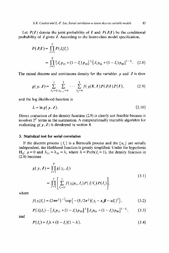
Let P(I) denote the joint probability of I and P( Jl1) be the conditional probability of J given I. According to the latent-class model specification,

= ~I~P,,+(l-J,)P,,l”[J,P,,+(l-J,)P,l’-”. w9 t=1

The mixed discrete and continuous density for the variables y and J is then

1 1 1

dy, J)= c c -.. I,=0 IT_,=0

and the log likelihood function is

L=lng(y, J). (2.10)

Direct evaluation of the density function (2.9) is clearly not feasible because it involves 2T terms in the summation. A computationally tractable algorithm for evaluating g( y, J) is developed in section 4.

3. Statistical test for serial correlation

If the discrete process { 1, } is a Bernoulli process and the { u, } are serially independent, the likelihood function is greatly simplified. Under the hypothesis H,: p =0 and hi, = A,, = X, where h = Prob(1, = l), the density function in (2.9) becomes

t=1

= li i f(Ytl% 4Pvd4)fvt) [

t=1 I,=0

where

(3.1)

f(xlZ,) = (2~o*)-‘exp( -(1/2a*)(y, - x,B - a1,)*},

wtl4)= [J&l +(1 -4hlwrP,, +G -J,hJ and

P( 1,) = ZJ + (1 - zJ(1 - h).

(3.2)

I, 2 (3.3)

(3.4)

84 S.R. Cosslett and L.-F. Lee, Serial correlation in latent discrete variable models

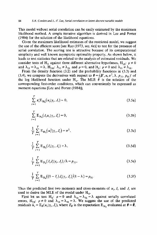
This model without serial correlation can be easily estimated by the maximum likelihood method. A simple iterative algorithm is derived in Lee and Porter (1984) for the solution of the likelihood equations.

Given the maximum likelihood estimates of the restricted model, we suggest the use of the efficient score [see Rao (1973, sec. 6e)] to test for the presence of serial correlation. The scoring test is attractive because of its computational simplicity and well known asymptotic optimality property. As shown below, it leads to test statistics that are related to the analysis of estimated residuals. We consider tests of H, against three different alternative hypotheses, HIS: p # 0 and h,, = A,, = h, H,,: X,, # A,, and p = 0, and H,: p it 0 and X,, # X,,.

From the density function (3.2) and the probability functions in (3.3) and (3.4), we compute the derivatives with respect to 8 = (/I’, cr, u2, A, pI1, poI)’ of the log likelihood function under H,. The MLE fi is the solution of the corresponding first-order conditions, which can conveniently be expressed as moment equations [Lee and Porter (1984)],

(3Sa)

f 2 EW,,($Iyt,JI)=u2, r=1

f c EH~(~IY,, 4) = A, t=1

+ i %,,((1-4)4~,~ 4,/O -A) =~ol. t=1

(3.5c)

(3Se)

(3.5f)

Thus the predicted first two moments and cross-moments of uI, Z, and J, are used to derive the MLE of the model under H,.

First let us test H,: p = 0 and A,, = A,, = h against serially correlated errors, H,,: p # 0 and A,, = X,, = A. We suggest the use of the predicted residuals fi, = EB(~.+~JJ~, J,), where E& is the expectation Err0 evaluated at 8 = 8,

S.R. Cosslert and L.-F. Lee, Serial correlation in latent discrete uariahle models 85

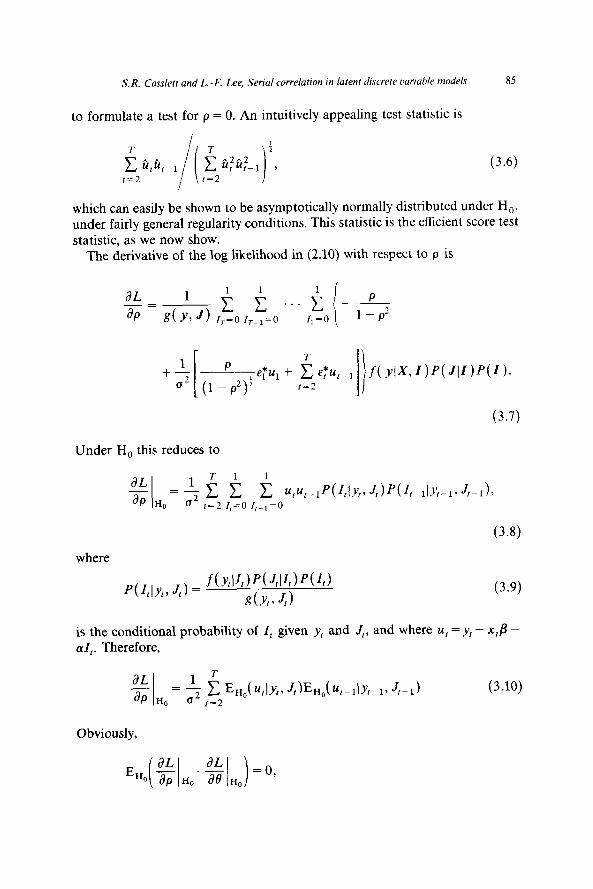
to formulate a test for p = 0. An intuitively appealing test statistic is

(34

which can easily be shown to be asymptotically normally distributed under H,, under fairly general regularity conditions. This statistic is the efficient score test statistic, as we now show.

The derivative of the log likelihood in (2.10) with respect to p is

l3L -= g(; q < i *‘* i aP , I, 0 1,_1=0 I, =o i

-&_

Under H, this reduces to

(3.8)

where

p(z ,y

t J) = f(Ytl~t)P(Jtl~t)P(Zt)

I, t dyt, Jt)

(3.9)

is the conditional probability of Z, given y, and J,, and where u, = y, - x,fi - aZt . Therefore,

aL = L i EH,bt~Y,, Jt)EH,b-~h~ J,-,>

%H, 0zt4 (3.10)

Obviously,

86 S. R. Cosslett and L. -F. Lee, Serial correlation in latent discrete vuriable models

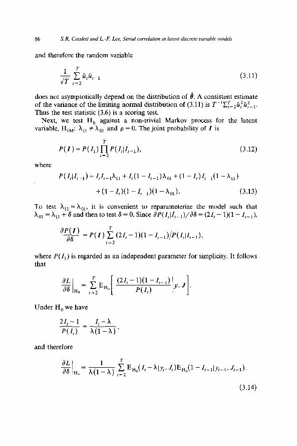
and therefore the random variable

(3.11)

does not asymptotically depend on the distribution of e. A consistent estimate of the variance of the limiting normal distribution of (3.11) is T-1ET=2C~fi~_1. Thus the test statistic (3.6) is a scoring test.

Next, we test H, against a non-trivial Markov process for the latent variable, HIM: Xi, # X,, and p = 0. The joint probability of I is

p(Z)=p(Z~)~~2p(Z~,Z~-~), (3.12)

where

P(Z*IZ,-1) =ZJ-iA,, + Z*(l - Z,-1)&i +(1 - ZJZt-10 -X,1)

+ (1 - Ml - Ll)O - h3,). (3.13)

To test hi, = Aoi, it is convenient to reparameterize the model such that X,, = A,, + 6 and then to test 6 = 0. Since aZ’(Z,lZ,_,)/LG = (21, - l)(l - Z1_i),

z$J = P(Z) i (21, - l)(l - Z,&(ZJI,_,), t=2

where P( Zi) is regarded as an independent parameter for simplicity. It follows that

a_c. T

as Ho= r=2EH” = [

wt- Nl -L1) y J I I fvt) ’ .

Under H, we have

2zt-1 z, - A _

p(4) h(l-h)’

and therefore

az. as Ho= ql! A> t$2EHotzt - A,.%, J,jEH,,cl - zt-l~~t-l~ J,-1).

(3.14)

S. R. Cosslett and L.-F. Lee, Serial correlation in latent discrete variable models 87

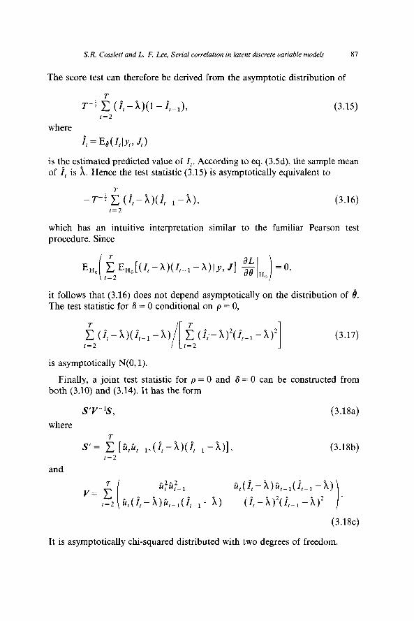
The score test can therefore be derived from the asymptotic distribution of

T-s 5 (1, -x)(1 - it& (3.15) t=2

where

it = Pe(Uvt, J,)

is the estimated predicted value of I,. According to eq. (3.5d), the sample mean of 1, is x. Hence the test statistic (3.15) is asymptotically equivalent to

-T-i c (it-i)(i,_,-A), (3.16)

which has an intuitive interpretation similar to the familiar Pearson test procedure. Since

‘%( ~E,~[(I,-h)(l,-,-h)l~,J] ~~Ho)=o, t=2

it follows that (3.16) does not depend asymptotically on the distribution of 6. The test statistic for 6 = 0 conditional on p = 0,

i (I,-^x)(i,_,-X) i (&4)‘(i,_,4)’ 1=2 ‘I t=2 1 (3.17)

is asymptotically N(0, 1).

Finally, a joint test statistic for p = 0 and 6 = 0 can be constructed from both (3.10) and (3.14). It has the form

S’V_‘S, (3.18a)

where

S’= i [i(ti(t~l,(it-x)(it_,-x)], (3.18b) t=2

and

-2-2 Ut Ut-1 ii,(i,-^x)a,_,(i,_, 3)

fi,(&x)n,_,(i,_, -1) i

(it-X)‘(i,_,-1)’

(3.18~)

It is asymptotically cm-squared distributed with two degrees of freedom.

88 S. R. Cossleti and L. -F. Lee, Serial correlation in latent discrete variable models

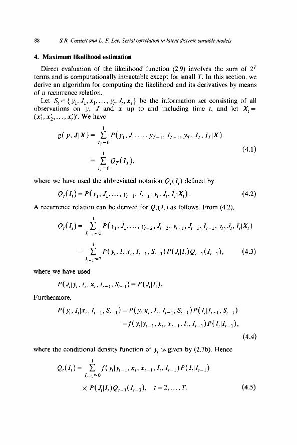
4. Maximum likelihood estimation

Direct evaluation of the likelihood function (2.9) involves the sum of 2= terms and is computationally intractable except for small T. In this section, we derive an algorithm for computing the likelihood and its derivatives by means of a recurrence relation.

Let S,= {.Y~,J~,~,..., y,, J,, xt} be the information set consisting of all observations on y, .Z and x up to and including time t, and let X, = ($&,..., xi)‘. We have

= joa,(

7-

(4.1)

where we have used the abbreviated notation Q,( Z,) defined by

Q,(~>=%Y,,J,,..., IL,, 4-1, Yt, 4, UXA. (4.2)

A recurrence relation can be derived for Q,(Z,) as follows. From (4.2),

Q,(4)= i P(Y~,J~,...,Y,-~,J~-~,Y,-~,JI-~,Z,-~,Y,,J,,Z,IX,) I,_,=0

= I,_~~P(~~,I,X,,I’-~, s,-,)P(J,lZ,)Q,~,(Z,-,),

where we have used

(4.3)

whb It, x,5 It-I, &I> = wtl4).

Furthermore,

where the conditional density function of y, is given by (2.7b). Hence

x P(J,lZ,)Q,_l(I,-l), t=L...,T. (4.5)

S. R. Cosslett and L.-F. Lee, Serial correlation in lutent discrete variable models 89

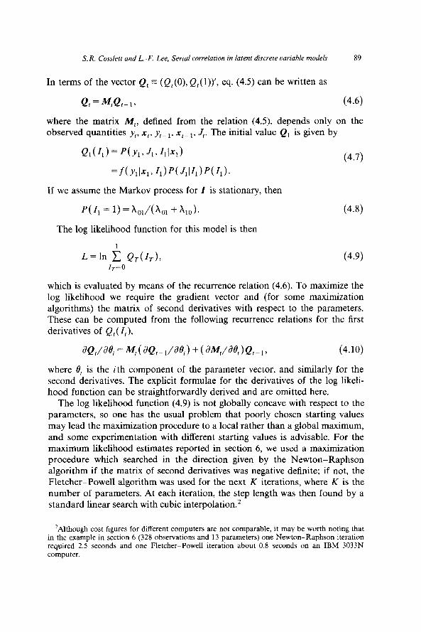
In terms of the vector Q, = (Q,(O), Q,(l))‘, eq. (4.5) can be written as

Q, = MB-1, (4.6)

where the matrix M,, defined from the relation (4.3, depends only on the observed quantities yt, xt, y,_,, x,-i,. I The initial value Qi is given by t.

Q,(4, = f’h 4,4I-d (4.7)

=f(YiI%Z1)WiIZi)P(Zi)*

If we assume the Markov process for I is stationary, then

P(Z, = 1) = W(&, + &J. (4.8)

The log likelihood function for this model is then

Z=ln i Q,(G), (4.9) lr=O

which is evaluated by means of the recurrence relation (4.6). To maximize the log likelihood we require the gradient vector and (for some maximization algorithms) the matrix of second derivatives with respect to the parameters. These can be computed from the following recurrence relations for the first derivatives of Q,( I,),

(4.10)

where S, is the i th component of the parameter vector, and similarly for the second derivatives. The explicit formulae for the derivatives of the log likeli- hood function can be straightforwardly derived and are omitted here.

The log likelihood function (4.9) is not globally concave with respect to the parameters, so one has the usual problem that poorly chosen starting values may lead the maximization procedure to a local rather than a global maximum, and some experimentation with different starting values is advisable. For the maximum likelihood estimates reported in section 6, we used a maximization procedure which searched in the direction given by the Newton-Raphson algorithm if the matrix of second derivatives was negative definite; if not, the Fletcher-Powell algorithm was used for the next K iterations, where K is the number of parameters. At each iteration, the step length was then found by a standard linear search with cubic interpolation.2

2Although cost figures for different computers are not comparable, it may be worth noting that in the example in section 6 (328 observations and 13 parameters) one Newton-Raphson iteration required 2.5 seconds and one Fletcher-Powell iteration about 0.8 seconds on an IBM 3033N computer.

90 S. R. Cosslett and L.-F. Lee. Serial correlation in latent discrete variable models

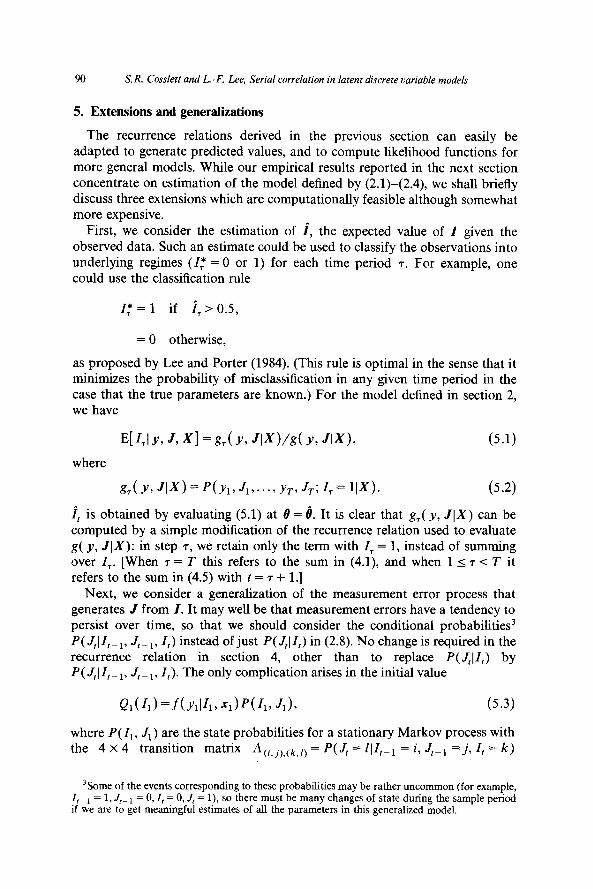
5. Extensions and generalizations

The recurrence relations derived in the previous section can easily be adapted to generate predicted values, and to compute likelihood functions for more general models. While our empirical results reported in the next section concentrate on estimation of the model defined by (2.1)-(2.4), we shall briefly discuss three extensions which are computationally feasible although somewhat more expensive.

First, we consider the estimation of i, the expected value of I given the observed data. Such an estimate could be used to classify the observations into underlying regimes (I,* = 0 or 1) for each time period T. For example, one could use the classification rule

I,*=1 if i,>O.5,

= 0 otherwise,

as proposed by Lee and Porter (1984). (This rule is optimal in the sense that it minimizes the probability of misclassification in any given time period in the case that the true parameters are known.) For the model defined in section 2, we have

E[ZA Y, J, Xl = d .v, JIX)/d Y, JlX>, (5.1)

where

s,(y> JIX)=P(y,,J,,...,y,,J,;Z,=lIX). (5.2)

il is obtained by evaluating (5.1) at B = 8. It is clear that g,( y, JlX) can be computed by a simple modification of the recurrence relation used to evaluate g( y, JIX): in step 7, we retain only the term with Z, = 1, instead of summing over Z,. [When 7 = T this refers to the sum in (4.1), and when 1 2 7 < T it refers to the sum in (4.5) with t = 7 + 1.1

Next, we consider a generalization of the measurement error process that generates J from I. It may well be that measurement errors have a tendency to persist over time, so that we should consider the conditional probabilities3 P( JIIZ,_l, J,_ 1, Z,) instead of just P(J,IZ~) in (2.8). No change is required in the recurrence relation in section 4, other than to replace P(J,IZt) by P( J,JZ,_l, J,_1, I,). The only complication arises in the initial value

(5.3)

where P( Z1, J1) are the state probabilities for a stationary Markov process with the 4 x 4 transition matrix A,;, j),Ck,,) = P(J, = ElZ,_, = i, J,_l =j, Z, = k)

%me of the events corresponding to these probabilities may be rather uncommon (for example, I,- 1 = 1, J,_ 1 = 0, J, = 0, J, = l), so there must be many changes of state during the sample period if we are to get meaningful estimates of all the parameters in this generalized model.

S. R. Cosslett and L.-F. Lee, Serial correlation in latent discrete variable models 91

P(Z, = klZ,_, = i). These state probabilities can be expressed in terms of the parameters of the model by a straightforward calculation. Thus maximum likelihood estimation is still feasible, although there are six additional parame- ters.

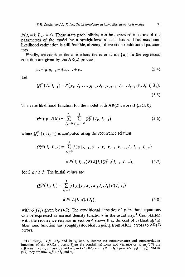
Finally, we consider the case where the error terms { ut } in the regression equation are given by the AR(2) process

Let

u, = @1&I + @zu,-z + Et. (5.4)

(5.5)

Then the likelihood function for the model with AR(2) errors is given by

d2’( y, 4X) = i i Q$%, I,-,), (5.6) IT=0 I,_,=0

where QP)(Z,, I,_ 1) is computed using the recurrence relation

for 3 I t I T. The initial values are

Q$2’(L 4) = i f(y2lyv ~23 ~,J2J,)f’(~2I4) I,=0

xW,lZ,)Q,(4), (5 4

with Qr(Z,) given by (4.7). The conditional densities of y, in these equations can be expressed as normal density functions in the usual way.4 Comparison with the recurrence relation in section 4 shows that the cost of evaluating the likelihood function has (roughly) doubled in going from AR(l) errors to AR(2) errors.

4Let u,=y, - x,B- d,, and let y, and p, denote the autocovariance and autocorrelation functions of the AR(2) process. Then the conditional mean and variance of y, in (5.7) are x,/I + al, + $Iu,_l + $P~u,-~ and a’; in (5.8) they are x2/I + alI + plu, and yO(l - p:); and in (4.7) they are now x1/3 + aI, and yo.

92 S.R. Cosslett and L.-E Lee, Serial correlation in latent discrete variable models

No further complexity (other than the proliferation of parameters) arises if we suppose that I, is also generated by a second-order process - we would just replace P(I$_,) by P(I,II,_,, It_2) in (5.7). The probabilities P(I,(I,_,) and P(I,) in (5.8) and (4.7) would then have to be expressed in terms of the state probabilities P(I, = i, I,_r =j) of a stationary Markov process with the 4 X 4 transition matrix Aci,j),(k, ,) = P(IZ = kll,_, = i, 11_2 =j)S,,, (where a,,,= 1 when i = 1 and I$, = 0 otherwise).

6. An empirical illustration

To illustrate the use of the test statistics given in section 3 and the estimation procedure described in section 4, we apply them to the data on cartel stability in Lee and Porter (1984). The sample consists of weekly time series data on the Joint Executive Committee (JEC) railroad cartel from week 1 in 1880 to week 16 in 1886. The problem is to study the price-setting behavior of the cartel and to test the proposition that observed ‘price wars’ represented a switch from collusive to non-cooperative behavior.

Let I, be a latent dichotomous variable which equals one when the industry is in a cooperative regime, and equals zero when the industry reverts to non-cooperative behavior, i.e., pricing at marginal cost. The discrete indicator variable, J,, is equal to one unless the Railway Review, a trade magazine, reported that a price war was occurring in week t. This indicator was reported in Ulen (1978). One reason why Lee and Porter suspected measurement error in J, is that it conflicts with an index of cartel adherence constructed by MacAvoy (1965).5

The continuous indicator is the price variable pI, which is an index of prices charged by member firms (the grain rate, in dollars per 100 lbs.) and was announced by the JEC. The price-setting equation, which is the structural equation of interest, was specified by Lee and Porter (1984) as

4

In PI = PO + I&L, + C Pl+jDEj, + aZt + it* (6.1) /=I

The exogenous variables, which explain some of the price variation over time, are dummy variables defined as follows:

L = 1 if the Great Lakes were open to navigation; 0 otherwise; DE, = 1 from week 18 in 1880 to week 10 in 1883; 0 otherwise (reflecting

entry by the Grand Trunk Railway); DE, = 1 from week 11 to week 25 in 1883; 0 otherwise (reflecting an addition

to the New York Central);

sMacAvoy’s index is an annual series. Since Lee and Porter used weekly data, it would be difficult to construct an additional indicator for their model from MacAvoy’s index.

S. R. Cosslert and L.-F. Lee, Serial correlation in latent discrete oariahle models

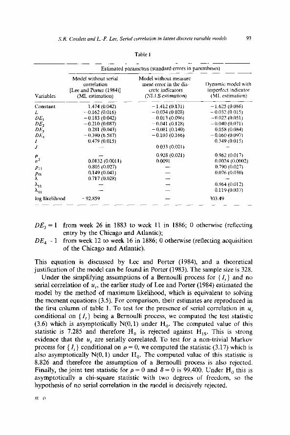
Table 1

93

Estimated parameters (standard errors in parentheses) - -

Variables

Model without serial correlation

[Lee and Porter (1984)] (ML estimation)

Model without measure- ment error in the dis-

Crete indicators (NLLS estimation)

constant ~ 1.474 (0.042) L -0.162 (0.016)

D-G - 0.183 (0.042)

DE, - 0.210 (0.087)

DE, - 0.281 (0.043)

DE, -0.390 (6.587) I 0.479 (0.015) J -

P a2

PI1

CO’ x 11 x 01

log likelihood

-

0.0132 (0.0011) 0.805 (0.027) 0.149 (0.041) 0.717 (0.028)

- 92.859

~ 1.412 (0.131) - 0.034 (0.028) - 0.013 (0.096) - 0.041 (0.128) -0.081 (0.140) -0.103 (0.166)

0.033 (0.021)

0.928 (0.021) 0.0091

-

Dynamic model with imperfect indicator

(ML estimation)

- 1.625 (0.086) - 0.032 (0.015) - 0.022 (0.051) - 0.040 (0.071) ~ 0.058 (0.084) - 0.060 (0.097)

0.349 (0.015)

0.962 (0.017) 0.0024 (0.0002) 0.790 (0.027) 0.076 (0.030)

-

0.964 (0.012) 0.119 (0.037)

303.49

DE, = 1 from week 26 in 1883 to week 11 in 1886; 0 otherwise (reflecting entry by the Chicago and Atlantic);

DE, = 1 from week 12 to week 16 in 1886; 0 otherwise (reflecting acquisition of the Chicago and Atlantic).

This equation is discussed by Lee and Porter (1984), and a theoretical justification of the model can be found in Porter (1983). The sample size is 328.

Under the simplifying assumptions of a Bernoulli process for {Z, } and no serial correlation of u,, the earlier study of Lee and Porter (1984) estimated the model by the method of maximum likelihood, which is equivalent to solving the moment equations (3.5). For comparison, their estimates are reproduced in the first column of table 1. To test for the presence of serial correlation in u, conditional on {I,} being a Bernoulli process, we computed the test statistic (3.6) which is asymptotically N(O,l) under H,. The computed value of this statistic is 7.285 and therefore H, is rejected against H,,. This is strong evidence that the u, are serially correlated. To test for a non-trivial Markov process for {I,} conditional on p = 0, we computed the statistic (3.17) which is also asymptotically N(0, 1) under Ha. The computed value of this statistic is 8.826 and therefore the assumption of a Bernoulli process is also rejected. Finally, the joint test statistic for p = 0 and 6 = 0 is 99.400. Under H, this is asymptotically a cm-square statistic with two degrees of freedom, so the hypothesis of no serial correlation in the model is decisively rejected.

JE D

94 S. R. Cosslett and L.-F. Lee, Serial correlation in latent discrete oanable models

Our recurrence relation algorithm is then used to estimate the model6 The MLE is reported in the third column of table 1. The lake dummy variable and the latent variable representing cooperative or non-cooperative behavior have a significant effect on price. In cooperative periods, i.e., I, = 1, the price was 42 percent higher than in non-cooperative periods.7 Equivalently, the price was cut 29 percent during price wars. When the lakes were open to navigation, the price was lower by 3.1 percent. The entry variables have negative coefficients as expected but are not significant, and the acquisition variable is also not significant. The estimate of pii is 0.79, which means that the Railway Review had reported collusion correctly in 79 percent of the cooperative periods. In about eight percent of the non-cooperative periods, the reports are incorrect.

The regime probability, h = Prob(1 = l), is X = h,,/(h,, + Xi,) under the assumption of stationarity. The estimate of A is 0.77, which means that in 77 percent of the sample periods the firms behaved cooperatively. The estimated transition probabilities imply strong state dependence: given that the previous period was cooperative, the probability is 0.96 that the following period is also cooperative, whereas the transition probability from non-cooperation to coop- eration is 0.12. The Markov model implies that the duration lengths have geometric probability distributions [see, e.g., Cox and Miller (1965)], and so the estimated mean durations are l/X,, = 27.8 periods for cooperation and l/X,, = 8.4 periods for non-cooperation. There is also strong positive serial correlation of the disturbances in the price equation. This evidence confirms the presence of dynamic structure in the price-setting mechanism.

We have also investigated the consequences of treating the regime indicators J as if they were perfect indicators for Z with no measurement error. Under this assumption, the price equation with serial correlation can be estimated by applying the nonlinear least squares (NLLS) method to the transformed eq. (2.5). The results are presented in the second column in table 1. No evidence was found of second-order autoregressive disturbances: NLLS estimation of the same model with u, = $iu,_r + &u,_~ + E, gave 6, = 0.952 (0.056). 6, = -0.026 (0.056) and negligible changes in the other parameter estimates in column 2. [This is only suggestive evidence against AR(2) disturbances, be- cause we reject the hypothesis of no measurement error. A formal test for AR(2) disturbances would require estimation of the more general model, using (5.6)-(5.8) to evaluate the likelihood.]

6The likelihood was maximized by the procedure described in section 4. Startmg values of the regression coefficients and of ptt and pu, were taken from the results of Lee and Porter. since those estimates should be consistent. Starting values of A,, and A,, were given by the sample transition rates of the indicator J,. Several ditferent starting values for the parameters were then tried, but no other maxima were found. When the steady-state probability (4.X) is used for the initial state, the search algorithm is sometimes unstable-with respect to A,,. and therefore the following nrocedure was used: the likelihood was first maximized holding P( I, = 1) fixed at the start&g value of X0,/(X,, + A,,): the result was then used as the starting point for a second search in which P( I, = 1) was allowed to vary with A,, according to (4.8).

‘This is computed from the ratio (P, - P,,)/P,, = eoi4’) - 1 = 0.4176 where P, is the expsctcd price when I = 1 and PO is the expected price when I = 0.

S. R. Cosslett and L.-F. Lee, Serial correlation in latent discrete variable models 95

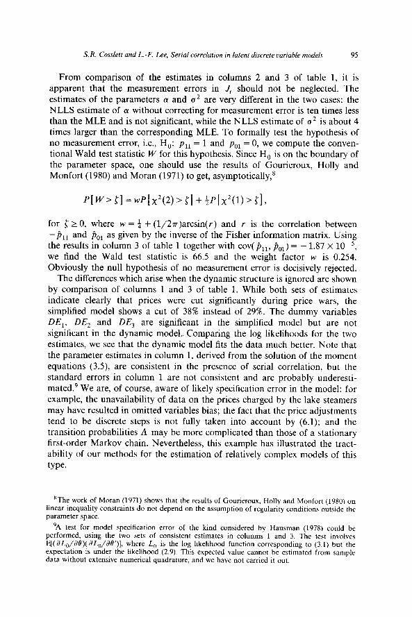
From comparison of the estimates in columns 2 and 3 of table 1, it is apparent that the measurement errors in J, should not be neglected. The estimates of the parameters (Y and a2 are very different in the two cases: the NLLS estimate of (Y without correcting for measurement error is ten times less than the MLE and is not significant, while the NLLS estimate of a2 is about 4 times larger than the corresponding MLE. To formally test the hypothesis of no measurement error, i.e., H,: pn = 1 and poI = 0, we compute the conven- tional Wald test statistic W for this hypothesis. Since H, is on the boundary of the parameter space, one should use the results of Gourieroux, Holly and Monfort (1980) and Moran (1971) to get, asymptotically,*

for 5 r 0, where w = a + (1/2r)arcsin(r) and Y is the correlation between --PI1 and joI as given by the inverse of the Fisher information matrix. Using the results in column 3 of table 1 together with cov( i)tl, &) = - 1.87 X 10m~5, we find the Wald test statistic is 66.5 and the weight factor w is 0.254. Obviously the null hypothesis of no measurement error is decisively rejected.

The differences which arise when the dynamic structure is ignored are shown by comparison of columns 1 and 3 of table 1. While both sets of estimates indicate clearly that prices were cut significantly during price wars, the simplified model shows a cut of 38% instead of 29%. The dummy variables DE,, DE, and DE, are significant in the simplified model but are not significant in the dynamic model.. Comparing the log likelihoods for the two estimates, we see that the dynamic model fits the data much better. Note that the parameter estimates in column 1, derived from the solution of the moment equations (3.5), are consistent in the presence of serial correlation, but the standard errors in column 1 are not consistent and are probably underesti- mated.’ We are, of course, aware of likely specification error in the model: for example, the unavailability of data on the prices charged by the lake steamers may have resulted in omitted variables bias; the fact that the price adjustments tend to be discrete steps is not fully taken into account by (6.1); and the transition probabilities A may be more complicated than those of a stationary first-order Markov chain. Nevertheless, this example has illustrated the tract- ability of our methods for the estimation of relatively complex models of this

type.

‘The work of Moran (1971) shows that the results of Gourieroux, Holly and Monfort (1980) on linear inequality constraints do not depend on the assumption of regularity conditions outside the parameter space.

9A test for model specification error of the kind considered by Hausman (1978) could be performed, using the two sets of consistent estimates in columns 1 and 3. The test involves E[(JL,/S7)( aL,/JO’)]. where Lo is the log likelihood function corresponding to (3.1) but the expectation is under the likelihood (2.9). This expected value cannot be estimated from sample data without extensive numerical quadrature, and we have not carried it out.

96 S. R. Cosslett and L.-F. Lee, Serial correlation in latent discrete variuble models

Appendix: Application to a Markov model of switching regressions

Consider the switching regression model

Y,: = xtsi + u,,, i=1,2, t=l,..., T, (A4

y,=yl*, if Z,=l,

(A.2) =y2: if Z,=O,

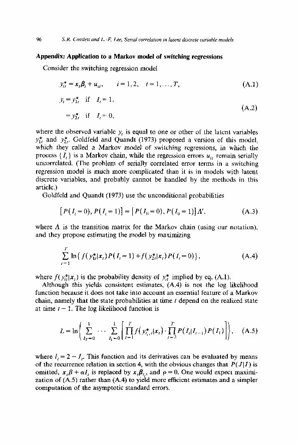
where the observed variable y, is equal to one or other of the latent variables yl*, and &. Goldfeld and Quandt (1973) proposed a version of this model, which they called a Markov model of switching regressions, in which the process {I,} is a Markov chain, while the regression errors z+, remain serially uncorrelated. (The problem of serially correlated error terms in a switching

regression model is much more complicated than it is in models with latent discrete variables, and probably cannot be handled by the methods in this

article.) Goldfeld and Quandt (1973) use the unconditional probabilities

[P(Z,=O),P(Zt=l)] = [P(Z,=O),P(Z,=l)]A~, (A-3)

where A is the transition matrix for the Markov chain (using our notation), and they propose estimating the model by maximizing

where f(~i’flx,) is the probability density of y;f implied by eq. (A.l). Although this yields consistent estimates, (A.4) is not the log likelihood

function because it does not take into account an essential feature of a Markov chain, namely that the state probabilities at time t depend on the realized state at time f - 1. The log likelihood function is

where 1, = 2 - I,. This function and its derivatives can be evaluated by means of the recurrence relation in section 4, with the obvious changes that P( J(Z) is omitted, xtp + cd, is replaced by x$,,, and p = 0. One would expect maximi- zaticn of (A.5) rather than (A.4) to yield more efficient estimates and a simpler computation of the asymptotic standard errors.

S. R. Cossleti and L.-F. Lee, Serial correlation in lateni discrete vanable models 91

References

Aigner, D.J., 1973, Regression with a binary independent variable subject to errors of observation, Journal of Econometrics 1, 49-60.

Cox, D.R. and H.D. Miller, 1965, The theory of stochastic processes (Methuen & Co., London). Goldfeld, SM. and R.E. Quandt, 1973, A Markov model for switching regressions, Journal of

Econometrics 1, 3-15. Goodman, L.A., 1974a, The analysis of systems of qualitative variables when some of the variables

are unobservable, Part I: A modified latent structure approach, American Journal of Sociology 79. 117991259.

Goodman, L.A., 1974b, Exploratory latent structure analysis using both identifiable and unidenti- fiable models, Biometrika 61, 215-231.

Gourieroux, C., A. Holly and A. Monfort, 1980, Kuhn-Tucker, likelihood ratio and Wald tests for nonlinear models with inequality constraints on the parameters, Unpublished discussion paper.

Haberman, S.J., 1979, Analysis of qualitative data, Vol. 2 (Academic Press, New York). Hausman, J.A., 1978, Specification tests in econometrics, Econometrica 46, 1251-1271. Lazarsfeld, P.F., 1950, The logical and mathematical foundation of latent structure analysis, in:

S.A. Stouffer, ed., Measurement and prediction (Wiley, New York). Lazarsfeld. P.F. and N.W. Henry, 1968, Latent structure analysis (Houghton Mifflin, Boston, MA). Lee, L.F. and R.H. Porter, 1984, Switching regression models with imperfect sample separation

information, Econometrica 52, 391-418. MacAvoy, P.W.. 1965, The economic effects of regulation (MIT Press, Cambridge, MA). Moran, P.A.P., 1971, Maximum-likelihood estimation in non-standard conditions, Proceedings of

the Cambridge Philosophical Society 70. 44-450. Mouchart. M. 1977, A regression model with an explanatory variable with is both binary and

subject to errors, in: D.J. Aigner and A.S. Goldberger, eds., Latent variables in socio-economic models (North-Holland, Amsterdam).

Porter, R.H., 1983, Optimal cartel trigger price strategies, Journal of Economic Theory 29, 313-338.

Quandt, R.E., 1972, A new approach to estimating switching regressions, Journal of American Statistical Association 67, 306-310.

Rao, C.R., 1973, Linear statistical inference and its applications, 2nd ed. (Wiley, New York). Ulen, T-S., 1978, Cartels and regulation, Unpublished Ph.D. dissertation (Stanford University,

Stanford, CA).