Serial correlation in high-frequency data and the link ... And Patnai… · Serial correlation in high-frequency data and the link with liquidity Susan Thomas Tirthankar Patnaik December

Serial correlation in high-frequency dataand the link with liquidity

Susan Thomas Tirthankar Patnaik

December 12, 2002

Abstract

This paper tests for market efficiency at high-frequencies of the Indian equity markets. Wedo this by testing the behaviour of serial correlation in firm stock prices using the VarianceRatio test on high frequency returns data. We find that at a frequency interval of five minutes,all the stocks show a pattern of mean-reversion. However, different stocks revert at differentrates. We find that there is a correlation between the time the stock takes to revert to the meanand the liquidity of the stock on the market. Here, liquidity is measured both in terms of impactcost as well as trading intensity.

Keywords: Variance-Ratios, High Frequency Data, Market Liquidity

Contents

1 Introduction 3

2 Issues 5

2.1 Choice of frequency for the price data . . . . . . . . . . . . . . . . . . . . . . . . 6

2.2 Concatenation of prices across different days . . . . . . . . . . . . . . . . . . . . 6

2.3 Intra-day heteroskedasticity in returns . . . . . . . . . . . . . . . . . . . . . . . . 7

2.4 Measuring intra-day liquidity . . . . . . . . . . . . . . . . . . . . . . . . . . . . . 7

3 Econometric strategies 8

3.1 The Variance Ratio methodology . . . . . . . . . . . . . . . . . . . . . . . . . . . 8

1

3.2 Variance Ratios with HF data . . . . . . . . . . . . . . . . . . . . . . . . . . . . . 10

3.3 Issues of inference . . . . . . . . . . . . . . . . . . . . . . . . . . . . . . . . . . 10

4 Data description 11

5 Results 13

5.1 Serial correlation in the Market Index . . . . . . . . . . . . . . . . . . . . . . . . 13

5.2 Serial correlations in individual stocks . . . . . . . . . . . . . . . . . . . . . . . . 16

6 Conclusion 21

2

1 Introduction

The earliest tests of the “Efficient Market Hypothesis” (EMH) have focussed on serial correlationin financial market data. The presence of significant serial correlation indicates that prices couldbe forecasted. This, in turn, implies that there might be opportunities for rational agents to earnabnormal profits if the forecasts were predictable after accounting for transactions costs. Under thenull of the EMH though, serial correlations ought to be neglible. Most of the empirical literatureon market efficiency documents that serial correlations in daily returns data are very small, whichsupports the hypothesis of market efficiency.

However, most of these tests are vulnerable to problems of low power. There are papers that pointout that tests of serial correlation are vulnerable to low power (Summers, 1986) given that:

• There is strong heteroskedasticity in the data.

• There are changes in the characteristics of the data caused by changes in the economic environment,changes in market microstructure, the presence of economic cycles, etc.

• The changes in the DGP can also impact upon the character of heteroskedasticity as well.

Therefore, the number of observations that are typically available at the monthly, weekly or evendaily levels usually lead to situations where the tests have weak power.

In the recent past, intra-day financial markets data has become available for analysis. Thishighfrequency data(HF data) constitutes price and volumes data that can be observed at intervals thatare as small as a second. The analysis of serial correlations with such high frequency data isparticularly interesting for several reasons.

One reason is that economic agents are likely to require time in order to react to opportunitiesfor abnormal profits that appear in the market during the trading day. While the time required foragents to react may not manifest themselves in returns observed at a horizon of a day, we mayobserve agents taking time to react as patterns of forecastability in intra-day high-frequency data.For example, one class of models explaining the behaviour of intra-day trade data are based on thepresence of asymmetric information between informed traders and uninformed traders. When alarge order hits the market, there will be temporary uncertainty about whether this is a speculativeorder placed by an informed trader, or a liquidity-motivated order placed by an uninformed trader.This phenomenon could generate short-horizon mean reversion in stock prices.

Another reason why HF data could prove beneficial for market efficiency studies is the sheer abun-dance of the data. This could yield highly powerful statistical tests of efficiency, that would besensitive enough to reject subtle deviations from the null. However, the use of HF data also in-troduces problems such as those of asynchronous data, especially in cross-sectional studies. Since

3

different stocks trade with different intensity, using HF data is constrained to not suffer too muchof a missing data problem across all the stocks in the sample.

In this paper, we study the behaviour of serial correlation of HF stock price returns from theNational Stock Exchange of India (NSE). We use variance ratio (VR) tests which was first appliedto financial data in Nelson and Plosser (1982). We study both the returns of the S & P CNX Nifty(Nifty) market index of the NSE, and to a set of 100 stocks that trade on the NSE. We choose thosestocks which are the most liquid stocks in India and which, therefore, have the least probability ofmissing data even at a very small intervals.

The literature leads us to expectpositive deviations from the meanin the index returns (Atchisonet al., 1987) andnegative serial correlationsin stocks (Roll, 1984). The positive correlation inindex returns is attributed to the asynchronous trading of the constituent index stocks: informationshocks would first impact on the prices of stocks that are more liquid (and therefore, more activelytraded) and impact on price of less active stocks with a lag. When the index returns are studied atvery short time intervals, this effect ought to be even more severe as compared to the correlationsin daily data with the positive serial correlations perhaps continuously growing for a period of timebefore returning to the mean (Low and Muthuswamy, 1996). The negative serial correlations instock returns is attributed to the “bid-ask bounce”: here, the probability of a trade executing atthe bid price being followed by a trade executing at the ask price is higher than a trade at the bidfollowed by another trade at the bid.

However, we find that there is no significant evidence of serial correlations in the index returns,even at an interval of five minutes. In fact, the VR at a lag of one is non-zero andnegative. Oneimplication is that there is no asynchronous trading within the constituent stocks of the index at afive-minute interval. Either we need to examine index returns at higher frequencies, in order to findevidence of asynchronous trading in the index or find an alternative factor to counter the positivecorrelations expected in a portfolio’s returns.

Our results on the VR behaviour of individual stocks is more consistent with the literature. All the100 stocks show significant negative deviations from the mean at a lag of five minutes. This meansthat stock returns at five minute intervals do have temporal dependance. However, there is a strongheterogeniety in the behaviour of the serial correlation across the 100 stocks. While the shortesttime to mean reversion is ten minutes, the longest is across several days!

While Roll (1984) shows how the liquidity measure of the bid-ask bounce can lead to negativeserial correlations in price, Hasbrouck (1991) shows that the smaller the bid-ask spread of thisstock, the smaller is the impact of a trade of a given size, which would lead to a smaller observedcorrelation in returns. Therefore, an illiquid stock with the same depth but larger spread wouldsuffer a larger serial correlation at the same lag. Thus, liquidity could have an impact not only onthesignof the serial correlation but also its magnitude. This, in turn, could affect the rate at whichthe VR reverts back to the mean.

4

The hypothesis is that the cross-sectional differences in serial correlation across stocks is drivenby the cross-sectional differences in their liquidity. We base our finding of heterogeniety in meanreversion as a test of this hypothesis.

The NSE disseminates the full limit order book information available for all listed stocks, ob-served at four times during the day. We construct the spread and theimpact costof a trade size ofRs.10,000 at each of these times for each of the stocks. We use the average impact cost as a mea-sure of intra-day liquidity of the stocks. We then construct deciles of the stocks by their liquidity,and examine the average VRs observed for each decile.

We find that the top decile by liquidity (ie, the most liquid stocks) have the smallest deviation frommean (in magnitude at the first lag). This decile also has the shortest time to mean reversion inVRs. The bottom decile by liqudity have the largest deviation from mean at the first lag as well asthe longest time to mean reversion. The pattern of increasing time to mean reversion is consistentlyobserved as correlated with decreasing liquidity as measured by the impact cost. Thus, we find thatthere is a strong correlation between mean reversion in returns of stocks and their liquidity.

The paper is organised as follows: Section 2 presents the issues in analysing intra-data of returnsas well as liquidity. In Section 3 focusses on developments in the VR methodology since Nelsonand Plosser (1982), and the method of inference we employ in this paper. We describe the datasetin Section 4. Section 5 presents the results, and we conclude our findings in Section 6.

2 Issues

High frequency finance is a relatively new field (Goodhart and O’Hara (1997), Dacorogna et al.(2001)). The first HF data that became available was the time series of every single traded price onthe New York Stock Exchange. The first studies of HF data were based on HF data from foreignexchange markets made available byOlsen and Associates. Studies based on these datasets werethe first to document time series patterns of intra-day returns and volatility. Wood et al. (1985),McNish (1993), Harris (1986), Lockwood and Linn (1990) were some of the first studies of theNYSE data, while Goodhart and Figliuoli (1991) and Guillaume et al. (1994) are some of thefirst papers on the foreign exchange markets. Since then, there have been several papers that haveworked on further characterising the behaviour of intra-day prices, returns and volumes of financialmarket data (Goodhart and O’Hara (1997), Baillie and Bollerslev (1990), Gavridis (1998), Dunis(1996), ap Gwilym et al. (1999)).

These papers raised several issues for consideration about peculiarities of HF data that are notpresent in the frequencies that have been traditionally analysed such as daily or weekly data. Thetwo issues that we had to deal with at the outset of our analysis of the Indian HF data were:

1. The issue of the frequency at which to analyse the data.

5

2. How to concatenate returns across days.

3. The problem of higher volumes/volatility at the start and at the end of every trading day.

2.1 Choice of frequency for the price data

Data observed from financial markets in real-time have the inherent problem of being irregular intraded frequency (Granger and Ding, 1994). Part of the problem arises because of the quality ofpublished data - trading systems at most exchanges can execute trades at finer intervals than thefrequency at which exchanges record and publish data. For example, the trading system at the NSEcan do trades at intervals of1/64th of a second. However, the data is published with timestamps atthe smallest interval of a second. There could be multiple trades within the same timestamp.

On the other hand, some stocks do trade with the intensity of several trades within a second,whereas other may do just one. Thus, the notion of the “last traded price” (LTP) for two dif-ferent stocks might actually mean prices at two different real times, which leads to comparingasynchronous orirregular data.1

However, when we study the cross-sectional behaviour of (say) serial correlation of stock prices,there is a need to synchronise the price data that is being studied. There are several methods ofsynchronising irregular data that is used in the literature. One approach is to model the time seriesof every stock directly in trade-time, rather than in clock or calendar time (Marinelli et al., 2001).Another approach is of Dacorogna et al. (2001), who follow a time-deformation technique calledν-time. Here, they model the time series as a subordinated process of another time series.

We follow the approach of Andersen and Bollerslev (1997) who impose a discrete-time grid onthe data. In this approach, the key parameter of choice is the width of the grid. If the width of theinterval is too high, then information about the temporal pattern in the returns may be lost. On theother hand, a thin interval may lead to high incidence of “non–trading” which is associated withspurious serial-correlation in the returns. Therefore, the grid interval must be chosen to minimizethe informational loss while avoiding the problem of spurious autocorrelation.

2.2 Concatenation of prices across different days

When intraday data is concatenated across days, the first return on any day is not really an intradayreturn from the previous time period, but anovernightreturn. This is asynchronous with the inter-

1For example, stock A at the NSE trades four times within the second, with trades at the1st, 2nd, 3rd and15th 64th

interval of a second. Stock B trades once with a trade at the63rd interval. Then the LTP recorded for A is at15/64th

of a second and B at63/64th of a second which is asynchronous in real time.

6

vals implied in other returns data. Returns over differing periods can lead to temporal aggregationproblems in the data, and result in spurious autocorrelation.

This is analogous to the practice of ignoring weekends when concatenating daily data. However,the same cannot be done for the intraday data. In the case of daily data, dropping the weekendmeans that every Monday is in reality a three-day return rather than a one-day return. However,the interval between the last return of a day and the first return on the next day will typically meana much larger number of intervals in the intervening period.2 Overnight returns have quite differentproperties as compared to intraday returns (Harris, 1986).

(Andersen and Bollerslev, 1997) solve this problem by dropping the first observation of everytrading day .

2.3 Intra-day heteroskedasticity in returns

Another issue that arises when analysing the serial correlations in the data are the U-shaped patternsin volumes and volatility. It is observed that returns in the beginning and the end of the tradingday tend to be different when compared with data from the mid-period of the trading day. Thismanifests itself in a U-shaped pattern of volatility. These patterns have been documented formarkets over the world (Wood et al. (1985); Stoll and Whaley (1990); Lockwood and Linn (1990);McNish and Wood (1990b,a, 1991, 1992); Andersen and Bollerslev (1997)).

If there are strong intraday seasonalities in HF data, then this could cause problems with ourinference of the serial correlations of returns. Andersen et al. (2001) regress the data using it’sFourier Flexible Formand analyse the behaviour of the residuals, rather than the raw data itself.

2.4 Measuring intra-day liquidity

Kyle (1985) characterises three aspects of liquidity: thespread, thedepthof the limit order book(LOB) and theresiliencywith which it reverts to its original level of liquidity. Papers from themarket microstructure literature have analysed the link between measures of liquidity and pricechanges. These start from Roll (1984) who established a link between the sign of the serial cor-relation to the bid-ask spread to Hasbrouck (1991) who established the depth of the LOB to themagnitude of the serial correlation and? who attempts to develop models of asymmetry of infor-mation to the resiliency of the LOB.

2For example, if we are using returns on a five minute interval, and the market closes at 4pm and opens at 10am, theinterval between the last return on one day and the opening return of the next day would mean a gap of 216 intervalsin between!

7

Typically, theory models change in liquidity measures as arising out of trades by informed oruninformed trades and the impact these trades on price changes. While there is no clear consensusfrom empirical tests on the precise role of information and the path through which it can impactupon prices through liquidity changes, there is consensus on the positive link between the effect ofliquidity upon serial correlation in stock returns (Hasbrouck (1991), Dufour and Engle (2000)).

The traditional metric used for real-time data on liquidity is the bid-ask spread that is availablefor many markets along with the traded price. Our dataset does not have real-time data on bid-ask spreads. Instead, we have access to two measures that capture liquidity:trading intensityandimpact cost.

• We define trading intensity as the number of trades in a given time interval of the trading day.It fluctuates in real-time and can either be measured either in value or in number of shares.

• Impact cost is the estimated cost of transacting a fixed value in either buying or selling astock. It is measured as the actual price paid (or received) with respect to the “fair price” ofthe stock, which is measured bybid + ask/2. The impact cost is calculated as

actual price/0.5 ∗ (bid + ask)

This measure is like the bid-ask spread but is a standardised measure which makes it directlycomparable across different stocks trading at different price levels. The impact cost is afunction of the size of the trade. It will depend upon the depth of the LOB and is a measureof the available liquidity of the stock. The impact cost is measured in basis points.

Both these liquidity measures are visible for an open electronic LOB. While the trading intensitycaptures the liquidity that has taken place thus far, the impact cost is a predictive measure ofliquidity. We will use both of these measures to test for the correlation between liquidity and serialcorrelations in HF data.

3 Econometric strategies

3.1 The Variance Ratio methodology

VRs have been often used to test for serial correlations in stock market prices (Lo and MacKinlay(1988),Poterba and Summers (1988)). The VR statistic measures the serial correlation overqperiod, as given by:

8

V R(q) =V ar[rt(q)]

V ar[rt], where rt(q) =

q∑k=1

rt (1)

= 1 +q−1∑k=1

(1− k

q

)ρk (2)

Here rt(q) is the q-period return, andρk is the k-period autocorrelation. For a random walk,ρk ≡ 0 ∀k. Hence the null of market efficiency is defined as,

V R(q) ≡ 1

which is what the value of the VR ought to be for a random walk.

The VR test has more power than the other tests for randomness, such as the Ljung-Box and theDickey-Fuller test (Lo and MacKinlay, 1989). It does not require the normality assumption, andis quite robust. Lo and MacKinlay (1988) derived the sampling distribution of the VR test statisticunder the null of a simple homoscedastic Random Walk (RW), and a more general uncorrelated butpossible heteroscedastic RW.3. The empirical literature on testing serial correlations in financialdata have largely used the heteroskedasticity consistent Lo and MacKinlay (1988) form.

There have been several papers extending and improving the tests of the VR: Chow and Denning(1993) extended the original form to jointly test multiple VRs, Cecchetti and sang Lam (1994)proposed a MonteCarlo method for exact inference when using a joint test of multiple VRs forsmall samples, Wright (2000) proposed exact tests of VRs based on the ranks and signs of timeseries, Pan et al. (1997) use a bootstrap scheme to obtain an empirical distribution of the VR ateachq.

One of the divides in the literature is on calculating VRs using overlapping data vs. non-overlappingdata. In the former, the aggregation of data overq periods is done using overlapping windows oflengthq, whereas in the latter the data is aggregated over windows of data that do not overlap. Ifthe time series is short, then overlapping windows re-use old data to give a larger number of pointsavailable to calculate the VR atq. However, the efficiency of this form of the VR estimator islower.

Richardson and Stock (1989) develop the theoretical distribution of both the overlapping and thenon-overlapping VR statistic: they show that the limiting distribution in the case of the overlappingstatistic is a chi-squared distribution that is robust to heteroskedasticity and non-normality. Thedistribution of the non-overlapping statistic is a functional of a Brownian Motion and can only beestimated using Monte Carlo. Richardson and Smith (1991) find that overlapping VRs have 22%higher standard errors compared with non-overlapping VRs.

3For more details on the various types of the RW that can be tested, see Campbell et al. (1997, Page. 28).

9

3.2 Variance Ratios with HF data

One of the earliest papers on the use of HF data in VR studies is Low and Muthuswamy (1996).They tested the serial correlations in quotes from three foreign exchange markets: USD/JPY,DEM/JPY, and USD/DEM for the period October 1992 to September 1993. They calculate vari-ance ratios for these FX returns where the holding period (aggregation) ranges from 5 minutes till3525 minutes (corresponding to 750 intervals).

They find that the VR do not immediately mean-revert - that negative correlation in the returnsbecomes stronger as the holding period increases. Variance Ratio (VR)s are found to grow faster inthe very short-runi.e., less than 200 minutes. This leads them to suggest that “serial dependenciesare stronger in the long-run”.

The use of the VR in the HF data literature has been relatively limited so far. But the existing workhighlight one interesting new facet of the issue of using over-lapping versus non-over-lapping datain VR studies when applied to HF data:

• The abundance of HF data and the lower efficiency of overlapping VR would imply that weshould use non-overlapping VRs to test for serial correlation in HF data.

• Andersen et al. (2001) study the shift in volatility patterns in HF data. They use non-overlapping returns to analyse the behaviour of the VR in this data. They show that thestandard VR tests could be seriously misleading when applied on intraday data, due tothe inherent intraday periodicity present. Thus, they suggest applying a Fourier FlexibleForm (FFF) Gallant (1981) when analyzing such data.

3.3 Issues of inference

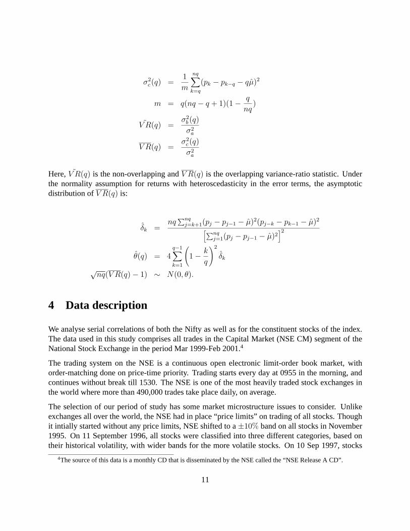
Lo and MacKinlay (1988) developed the heteroskedasticity-consistent overlapping VR statistic. Ifthe sample of HF prices has T observations and we need to calculate the VR at an aggregation ofq, then:

µ̂ =1

nq

nq∑k=1

(pk − pk−1)

σ2a =

1

nq − 1

nq∑k=1

(pk − pk−1 − µ̂)2

σ2b (q) =

1

m

nq∑k=q

(pqk − pqk−q − qµ̂)2

10

σ2c (q) =

1

m

nq∑k=q

(pk − pk−q − qµ̂)2

m = q(nq − q + 1)(1− q

nq)

˜V R(q) =σ2

b (q)

σ2a

V R(q) =σ2

c (q)

σ2a

Here, ˜V R(q) is the non-overlapping andV R(q) is the overlapping variance-ratio statistic. Underthe normality assumption for returns with heteroscedasticity in the error terms, the asymptoticdistribution ofV R(q) is:

δ̂k =nq∑nq

j=k+1(pj − pj−1 − µ̂)2(pj−k − pk−1 − µ̂)2[∑nqj=1(pj − pj−1 − µ̂)2

]2θ̂(q) = 4

q−1∑k=1

(1− k

q

)2

δ̂k

√nq(V R(q)− 1) ∼ N(0, θ).

4 Data description

We analyse serial correlations of both the Nifty as well as for the constituent stocks of the index.The data used in this study comprises all trades in the Capital Market (NSE CM) segment of theNational Stock Exchange in the period Mar 1999-Feb 2001.4

The trading system on the NSE is a continuous open electronic limit-order book market, withorder-matching done on price-time priority. Trading starts every day at 0955 in the morning, andcontinues without break till 1530. The NSE is one of the most heavily traded stock exchanges inthe world where more than 490,000 trades take place daily, on average.

The selection of our period of study has some market microstructure issues to consider. Unlikeexchanges all over the world, the NSE had in place “price limits” on trading of all stocks. Thoughit intially started without any price limits, NSE shifted to a±10% band on all stocks in November1995. On 11 September 1996, all stocks were classified into three different categories, based ontheir historical volatility, with wider bands for the more volatile stocks. On 10 Sep 1997, stocks

4The source of this data is a monthly CD that is disseminated by the NSE called the “NSE Release A CD”.

11

were again classified into three categories, this time based on liquidity, with wider bands for themore liquid stocks. A series of changes in the price-limits of stocks have followed since then.In March 2001, the exchange changed over to a rolling settlement system. Further, there have anumber of changes in the trading-times of the exchange over the years. For the period under study,the exchange traded in the interval 0955:1530.

We select March 1999 to February 2001 as our period of study because this period has the leastmicrostructural changes to the price discovery on the exchange. A total of 1384 stocks traded inthis period. The data set has about 253,717,939 records in 514 days. These are “time and sales”data, (as defined in MacGregor (1999)).

We deal with the issues raised in Section 2 in the following manner:

Selection of data frequencyWe have chosen a 300 second interval as the base frequency for thisgrid. Our choice is based on various tests and diagnostic measures (Patnaik and Shah, 2002).The 300s discretization gives about 67 data points per day. On average, we observe that at a300 second interval, there is an incidence of 10% missing observations.

In addition, the data were filtered of outliers, and anomalous observations. An outlier ob-servation results when a trade is recorded for a stock, outside it’s price band. Anomalousobservations could be caused when the position of the decimal point is misplaced whilerecording the data. Errors range from incorrect recording, to human errors. A number ofpapers have dealt with the issues of cleaning up and filtering of intraday data (Dacorognaet al., 2001). The specifics of data-filtering and cleaning for HF data from the NSE can befound in Patnaik and Shah (2002).

Concatenation of data across different daysWe follow the solution adopted by Andersen andBollerslev (1997) of ignoring the first return in the day, andthen concatenating the data.

Trading intensity NSE has one of the highest trading intensities in the world. In this period stud-ied here, the mean trading intensity was about 24.56 trades per second.5 For the study, wechose the hundred most traded stocks in the period. On an average, each of these stockstraded about 4211 times a day, about one trade in every 5 seconds. These 100 stocks com-prise about 83.32% of all the trades recorded in this period at the NSE.

Calculation of intra-day impact costs The impact cost for a stock is calculated using order-booksnapshots of the market which are recorded four times a day by the National Stock Exchange(NSE), at 1100, 1200, 1300, and 1400 respectively. The complete Market By Price (MBP)6

5253717939 trades over 514 days, with 20100 trading seconds in a day, gives 24.56.6This is the set of all the limit orders that are available in the market at that time, both on the buy and on the sell

side. Since the limit order shows both the price and the quantity, it is easy to calculate the impact cost for any stockgiven a certain size of the trade. Given the MBP we can calculate the graph of the impact cost at all trade sizes for agiven stock. This graph is called the liquidity supply schedule and is always empirically different for the buy and thesell side of the LOB.

12

is available at these times.

For our study, we calculate the buy/sell impact cost for an order of Rs. 10,000 for each ofthe 1382 stocks that traded in the sampling period. The calculation was done for the LOBdata for each of the four time points for every traded day in this period. We then selectd the100 most liquid stocks on the basis of mean buy and sell impact cost.7

We show the top and bottom ten stocks by liquidity by both the impact cost and the trading intensitymeasures in Table 1. We can see that that the most liquid stock is RELIANCE, with an impact costof 7 basis points for a transaction size of Rs.10,000, and the least liquid stock is CORPBANK witha median impact cost of 26 basis points for the same transaction size.

There appears also some amount of difference in the ordering by the two liquidity measures. How-ever, at level of quartiles of stocks, the differences are not significant.

5 Results

We estimate the overlapping VRs for the NSE-50 index as well as all the 100 stocks in our sample.We depict the results as a set of two graphs for each of the returns:

1. The first graph shows the VRs themselves starting from an aggregation of two (which is theserial correlation for returns at ten minute intervals) and continues upto an aggregation of350 lags (which is the serial correlation of returns at one trading week or five days).

The null that we test is that if the returns are truly random, then the VRs should be notsignificantly different from a value of one. The graph shows two sets of confidence intervals,the inner intervals are for the 95% band and the outer ones are for the 99% bands.

2. The second graph shows the non-overlapping heteroskedasticity consistent VR statistic.Once again, the statistic is plotted for aggregation levels from two to 350. The null impliesthat the statistic should have a value of 0. Both the 95% and the 99% confidence intervalsare drawn around the statistics.

The graphs for the NSE-50 index and the stocks are shown below.

5.1 Serial correlation in the Market Index

We find that the index shows no pattern of significant serial correlations even at the five-minuteinterval as can be seen in Figure 1.

7The list of all the 100 stocks is in the appendix.

13

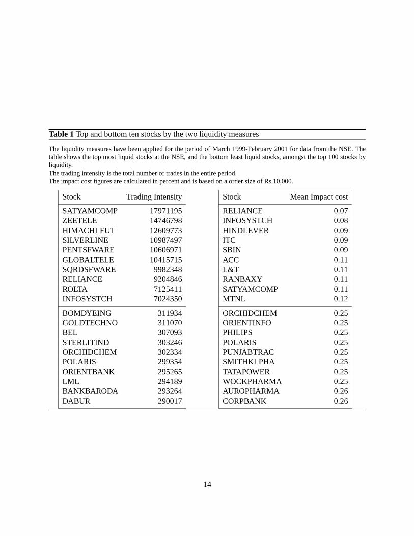
Table 1Top and bottom ten stocks by the two liquidity measures

The liquidity measures have been applied for the period of March 1999-February 2001 for data from the NSE. Thetable shows the top most liquid stocks at the NSE, and the bottom least liquid stocks, amongst the top 100 stocks byliquidity.The trading intensity is the total number of trades in the entire period.The impact cost figures are calculated in percent and is based on a order size of Rs.10,000.

Stock Trading Intensity Stock Mean Impact cost

SATYAMCOMP 17971195 RELIANCE 0.07ZEETELE 14746798 INFOSYSTCH 0.08HIMACHLFUT 12609773 HINDLEVER 0.09SILVERLINE 10987497 ITC 0.09PENTSFWARE 10606971 SBIN 0.09GLOBALTELE 10415715 ACC 0.11SQRDSFWARE 9982348 L&T 0.11RELIANCE 9204846 RANBAXY 0.11ROLTA 7125411 SATYAMCOMP 0.11INFOSYSTCH 7024350 MTNL 0.12

BOMDYEING 311934 ORCHIDCHEM 0.25GOLDTECHNO 311070 ORIENTINFO 0.25BEL 307093 PHILIPS 0.25STERLITIND 303246 POLARIS 0.25ORCHIDCHEM 302334 PUNJABTRAC 0.25POLARIS 299354 SMITHKLPHA 0.25ORIENTBANK 295265 TATAPOWER 0.25LML 294189 WOCKPHARMA 0.25BANKBARODA 293264 AUROPHARMA 0.26DABUR 290017 CORPBANK 0.26

14

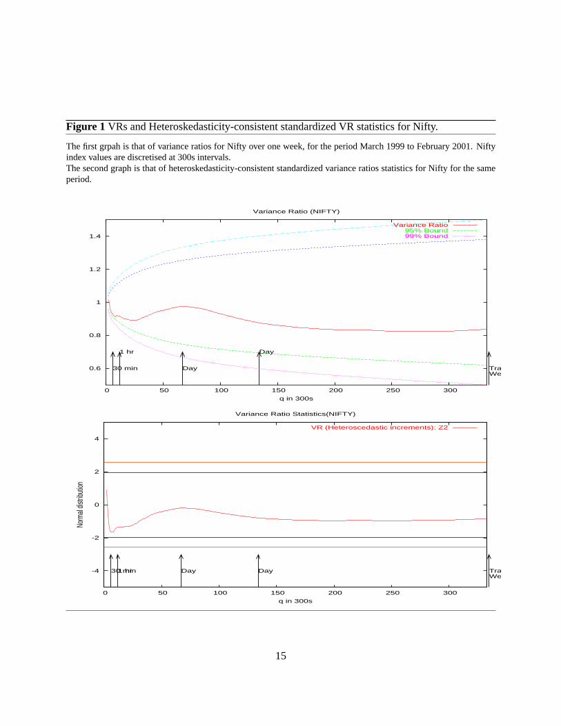
Figure 1 VRs and Heteroskedasticity-consistent standardized VR statistics for Nifty.

The first grpah is that of variance ratios for Nifty over one week, for the period March 1999 to February 2001. Niftyindex values are discretised at 300s intervals.The second graph is that of heteroskedasticity-consistent standardized variance ratios statistics for Nifty for the sameperiod.

0.6

0.8

1

1.2

1.4

0 50 100 150 200 250 300

q in 300s

Variance Ratio (NIFTY)

30 min

1 hr

Day

Day

TradingWeek

TradingMonth

TradingMonth

Variance Ratio95% Bound99% Bound

-4

-2

0

2

4

0 50 100 150 200 250 300

Norm

al dis

tributi

on

q in 300s

Variance Ratio Statistics(NIFTY)

30 min1 hr Day Day TradingWeek

TradingMonth

TradingMonth

VR (Heteroscedastic increments): Z2

15

This is contrary to what is documented in the literature where stock market indexes show “positive”correlations even in studies based on daily data. In this case, the very first VR is slightly aboveone, but the next three values are negative.

This is an interesting paradox to the typical rationale that is given to explain the behaviour ofintra-day index returns, which is the asynchronous trading of the constituent stocks. If the NSE-50 index shows negative correlations at the five-minute intervals, that could mean that there is somuch negative correlation that it beats the positive aspect we expect from asynchronous trading.

The other interesting aspect is that the Z-stats are significant if we ignore heteroskedasticity butare insignificant when we take heteroskedasticity into account. We infer therefore that the serialcorrelation patterns in the VR values are being driven largely by the intra-day U-shaped patternof volatility. However, there does not appear to be any serial correlations net of these intra-daypatterns.

5.2 Serial correlations in individual stocks

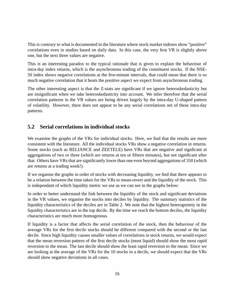
We examine the graphs of the VRs for individual stocks. Here, we find that the results are moreconsistent with the literature. All the individual stocks VRs show a negative correlation in returns.Some stocks (such as RELIANCE and ZEETELE) have VRs that are negative and signficant ataggregations of two or three (which are returns at ten or fifteen minutes), but not significant afterthat. Others have VRs that are significantly lower than one even beyond aggregations of 350 (whichare returns at a trading week!).

If we organise the graphs in order of stocks with decreasing liquidity, we find that there appears tobe a relation between the time taken for the VRs to mean-revert and the liquidity of the stock. Thisis independant of which liquidity metric we use as we can see in the graphs below:

In order to better understand the link between the liquidity of the stock and significant deviationsin the VR values, we organise the stocks into deciles by liquidity. The summary statistics of theliquidity characteristics of the deciles are in Table 2. We note that the highest heterogeniety in theliquidity characteristics are in the top decile. By the time we reach the bottom deciles, the liquiditycharacteristics are much more homogenous.

If liquidity is a factor that affects the serial correlation of the stock, then the behaviour of theaverage VRs for the first decile stocks should be different compared with the second or the lastdecile. Since high liquidity causes smaller values of correlations in stock returns, we would expectthat the mean reversion pattern of the first decile stocks (most liquid) should show the most rapidreversion to the mean. The last decile should show the least rapid reversion to the mean. Since weare looking at the average of the VRs for the 10 stocks in a decile, we should expect that the VRsshould show negative deviations in all cases.

16

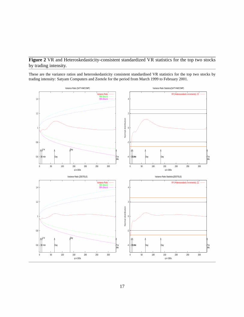
Figure 2 VR and Heteroskedasticity-consistent standardized VR statistics for the top two stocksby trading intensity.

These are the variance ratios and heteroskedasticity consistent standardised VR statistics for the top two stocks bytrading intensity: Satyam Computers and Zeetele for the period from March 1999 to February 2001.

0.6

0.8

1

1.2

1.4

0 50 100 150 200 250 300

q in 300s

Variance Ratio (SATYAMCOMP)

30 min

1 hr

Day

Day

TradingWeek

TradingMonth

TradingMonth


-4

-2

0

2

4

0 50 100 150 200 250 300

No

rma

l d

istr

ibu

tio

n

q in 300s

Variance Ratio Statistics(SATYAMCOMP)


TradingMonth

TradingMonth


0.6

0.8

1

1.2

1.4

0 50 100 150 200 250 300

q in 300s

Variance Ratio (ZEETELE)

30 min

1 hr

Day

Day

TradingWeek

TradingMonth

TradingMonth


-4

-2

0

2

4

0 50 100 150 200 250 300

No

rma

l d

istr

ibu

tio

n

q in 300s

Variance Ratio Statistics(ZEETELE)


TradingMonth

TradingMonth


17

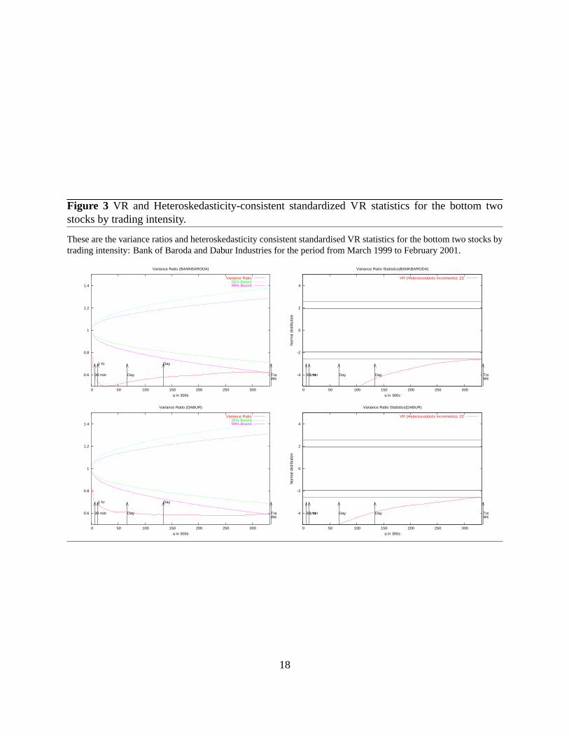
Figure 3 VR and Heteroskedasticity-consistent standardized VR statistics for the bottom twostocks by trading intensity.

These are the variance ratios and heteroskedasticity consistent standardised VR statistics for the bottom two stocks bytrading intensity: Bank of Baroda and Dabur Industries for the period from March 1999 to February 2001.

0.6

0.8

1

1.2

1.4

0 50 100 150 200 250 300

q in 300s

Variance Ratio (BANKBARODA)

30 min

1 hr

Day

Day

TradingWeek

TradingMonth

TradingMonth


-4

-2

0

2

4

0 50 100 150 200 250 300

Nor

mal

dis

trib

utio

n

q in 300s

Variance Ratio Statistics(BANKBARODA)


TradingMonth

TradingMonth


0.6

0.8

1

1.2

1.4

0 50 100 150 200 250 300

q in 300s

Variance Ratio (DABUR)

30 min

1 hr

Day

Day

TradingWeek

TradingMonth

TradingMonth


-4

-2

0

2

4

0 50 100 150 200 250 300

Nor

mal

dis

trib

utio

n

q in 300s

Variance Ratio Statistics(DABUR)


TradingMonth

TradingMonth


18

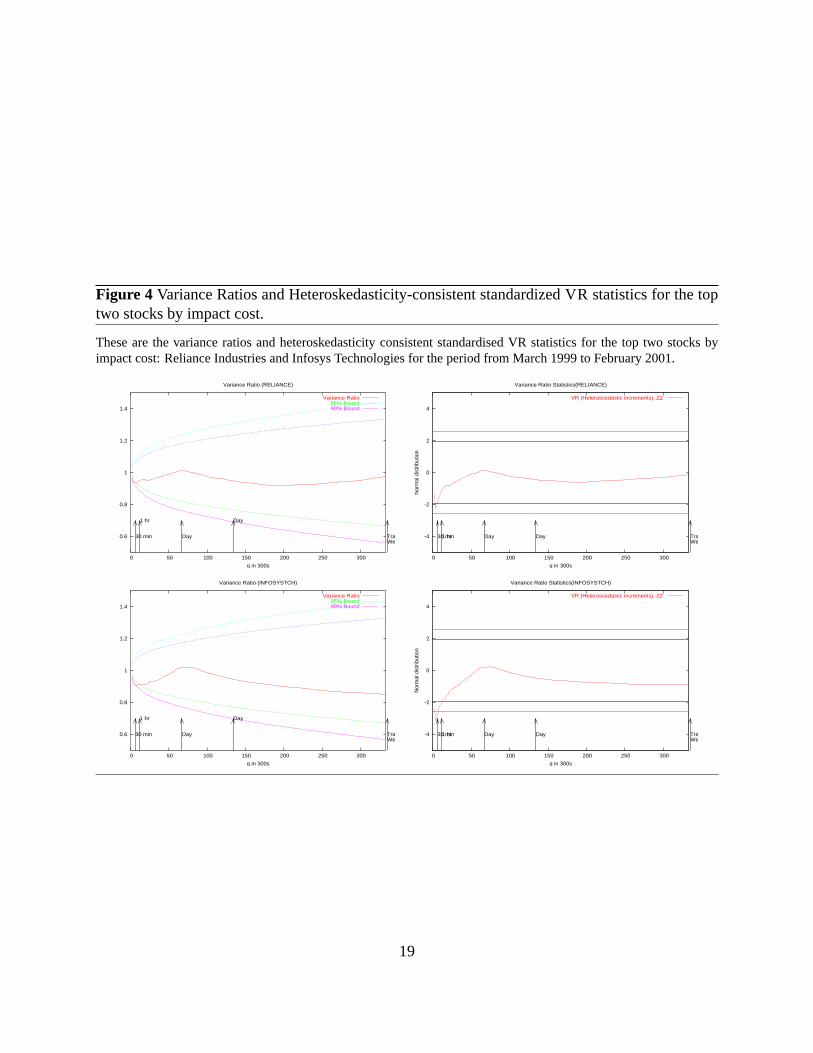
Figure 4 Variance Ratios and Heteroskedasticity-consistent standardized VR statistics for the toptwo stocks by impact cost.

These are the variance ratios and heteroskedasticity consistent standardised VR statistics for the top two stocks byimpact cost: Reliance Industries and Infosys Technologies for the period from March 1999 to February 2001.

0.6

0.8

1

1.2

1.4

0 50 100 150 200 250 300

q in 300s

Variance Ratio (RELIANCE)

30 min

1 hr

Day

Day

TradingWeek

TradingMonth

TradingMonth


-4

-2

0

2

4

0 50 100 150 200 250 300

Nor

mal

dis

trib

utio

n

q in 300s

Variance Ratio Statistics(RELIANCE)


TradingMonth

TradingMonth


0.6

0.8

1

1.2

1.4

0 50 100 150 200 250 300

q in 300s

Variance Ratio (INFOSYSTCH)

30 min

1 hr

Day

Day

TradingWeek

TradingMonth

TradingMonth


-4

-2

0

2

4

0 50 100 150 200 250 300

Nor

mal

dis

trib

utio

n

q in 300s

Variance Ratio Statistics(INFOSYSTCH)


TradingMonth

TradingMonth


19

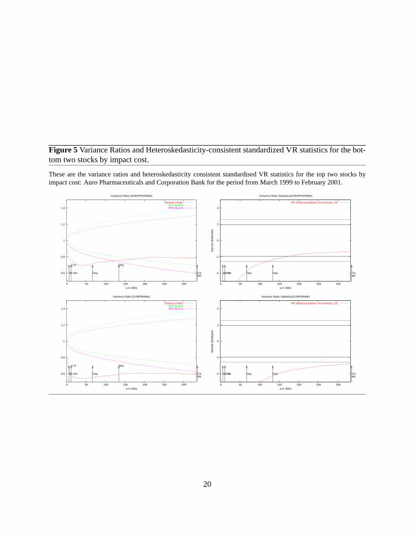
Figure 5 Variance Ratios and Heteroskedasticity-consistent standardized VR statistics for the bot-tom two stocks by impact cost.

These are the variance ratios and heteroskedasticity consistent standardised VR statistics for the top two stocks byimpact cost: Auro Pharmaceuticals and Corporation Bank for the period from March 1999 to February 2001.

0.6

0.8

1

1.2

1.4

0 50 100 150 200 250 300

q in 300s

Variance Ratio (AUROPHARMA)

30 min

1 hr

Day

Day

TradingWeek

TradingMonth

TradingMonth


-4

-2

0

2

4

0 50 100 150 200 250 300

Nor

mal

dis

trib

utio

n

q in 300s

Variance Ratio Statistics(AUROPHARMA)


TradingMonth

TradingMonth


0.6

0.8

1

1.2

1.4

0 50 100 150 200 250 300

q in 300s

Variance Ratio (CORPBANK)

30 min

1 hr

Day

Day

TradingWeek

TradingMonth

TradingMonth


-4

-2

0

2

4

0 50 100 150 200 250 300

Nor

mal

dis

trib

utio

n

q in 300s

Variance Ratio Statistics(CORPBANK)


TradingMonth

TradingMonth


20

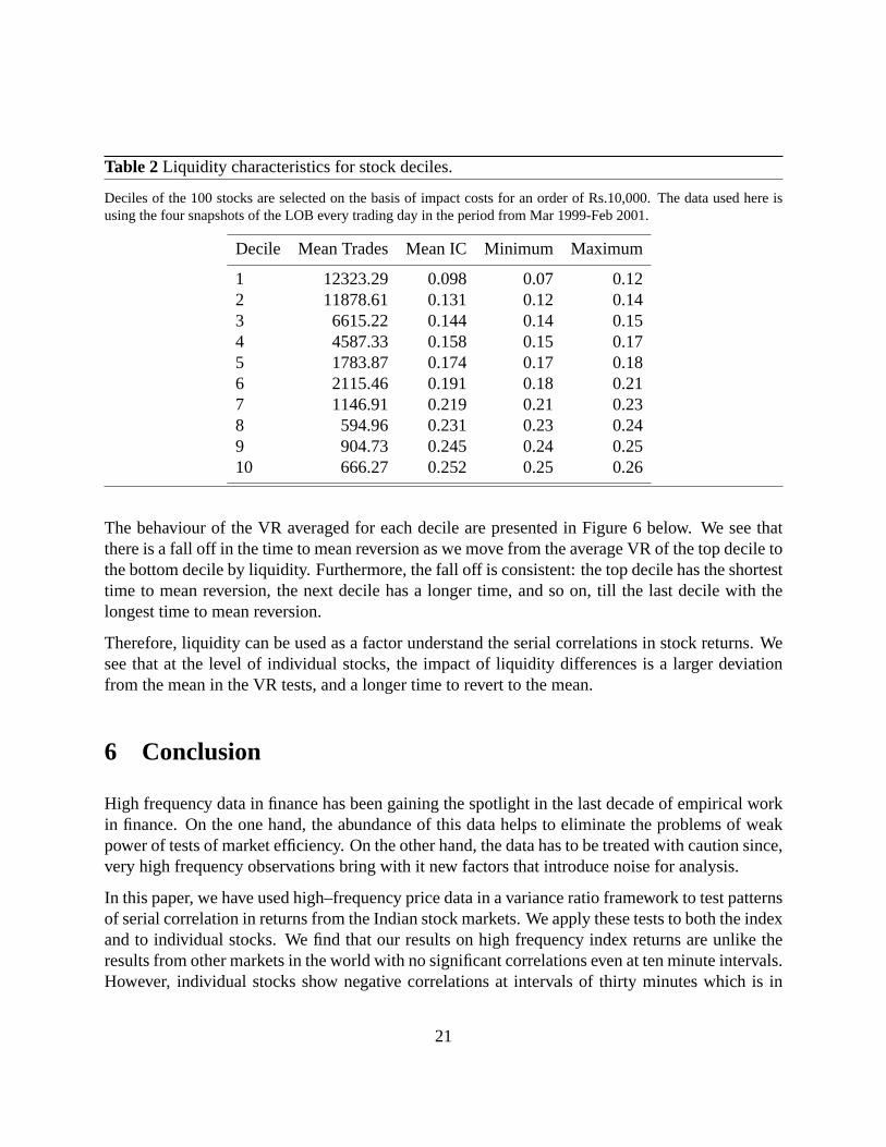
Table 2Liquidity characteristics for stock deciles.

Deciles of the 100 stocks are selected on the basis of impact costs for an order of Rs.10,000. The data used here isusing the four snapshots of the LOB every trading day in the period from Mar 1999-Feb 2001.

Decile Mean Trades Mean IC Minimum Maximum

1 12323.29 0.098 0.07 0.122 11878.61 0.131 0.12 0.143 6615.22 0.144 0.14 0.154 4587.33 0.158 0.15 0.175 1783.87 0.174 0.17 0.186 2115.46 0.191 0.18 0.217 1146.91 0.219 0.21 0.238 594.96 0.231 0.23 0.249 904.73 0.245 0.24 0.2510 666.27 0.252 0.25 0.26

The behaviour of the VR averaged for each decile are presented in Figure 6 below. We see thatthere is a fall off in the time to mean reversion as we move from the average VR of the top decile tothe bottom decile by liquidity. Furthermore, the fall off is consistent: the top decile has the shortesttime to mean reversion, the next decile has a longer time, and so on, till the last decile with thelongest time to mean reversion.

Therefore, liquidity can be used as a factor understand the serial correlations in stock returns. Wesee that at the level of individual stocks, the impact of liquidity differences is a larger deviationfrom the mean in the VR tests, and a longer time to revert to the mean.

6 Conclusion

High frequency data in finance has been gaining the spotlight in the last decade of empirical workin finance. On the one hand, the abundance of this data helps to eliminate the problems of weakpower of tests of market efficiency. On the other hand, the data has to be treated with caution since,very high frequency observations bring with it new factors that introduce noise for analysis.

In this paper, we have used high–frequency price data in a variance ratio framework to test patternsof serial correlation in returns from the Indian stock markets. We apply these tests to both the indexand to individual stocks. We find that our results on high frequency index returns are unlike theresults from other markets in the world with no significant correlations even at ten minute intervals.However, individual stocks show negative correlations at intervals of thirty minutes which is in

21

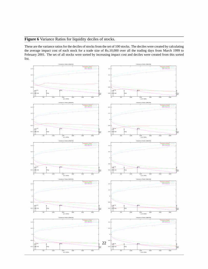
Figure 6 Variance Ratios for liquidity deciles of stocks.

These are the variance ratios for the deciles of stocks from the set of 100 stocks. The deciles were created by calculatingthe average impact cost of each stock for a trade size of Rs.10,000 over all the trading days from March 1999 toFebruary 2001. The set of all stocks were sorted by increasing impact cost and deciles were created from this sortedlist.

0.6

0.8

1

1.2

1.4

0 50 100 150 200 250 300

q in 300s

Variance Ratio (MEAN)

30 min

1 hr

Day

Day

TradingWeek

TradingMonth

TradingMonth


0.6

0.8

1

1.2

1.4

0 50 100 150 200 250 300

q in 300s


30 min

1 hr

Day

Day

TradingWeek

TradingMonth

TradingMonth


0.6

0.8

1

1.2

1.4

0 50 100 150 200 250 300

q in 300s


30 min

1 hr

Day

Day

TradingWeek

TradingMonth

TradingMonth


0.6

0.8

1

1.2

1.4

0 50 100 150 200 250 300

q in 300s


30 min

1 hr

Day

Day

TradingWeek

TradingMonth

TradingMonth


0.6

0.8

1

1.2

1.4

0 50 100 150 200 250 300

q in 300s


30 min

1 hr

Day

Day

TradingWeek

TradingMonth

TradingMonth


0.6

0.8

1

1.2

1.4

0 50 100 150 200 250 300

q in 300s


30 min

1 hr

Day

Day

TradingWeek

TradingMonth

TradingMonth


0.6

0.8

1

1.2

1.4

0 50 100 150 200 250 300

q in 300s


30 min

1 hr

Day

Day

TradingWeek

TradingMonth

TradingMonth


0.6

0.8

1

1.2

1.4

0 50 100 150 200 250 300

q in 300s


30 min

1 hr

Day

Day

TradingWeek

TradingMonth

TradingMonth


0.6

0.8

1

1.2

1.4

0 50 100 150 200 250 300

q in 300s


30 min

1 hr

Day

Day

TradingWeek

TradingMonth

TradingMonth


0.6

0.8

1

1.2

1.4

0 50 100 150 200 250 300

q in 300s


30 min

1 hr

Day

Day

TradingWeek

TradingMonth

TradingMonth


22

accordance with the literature from other markets.

One aspect of the individual stock correlations is the high degree of heterogeneity of mean rever-sion that we see across the set of 100 stocks. We analyse the heterogeniety in serial correlationsin terms of heterogeneity of liquidity and find there is substantial evidence of a link between theserial correlation and the liquidity in stock returns. We find that the average variance ratios acrossa decile of stocks with the best liquidity reverts to mean at a much more rapid rate (thirty minutes)as compared with that observed for the decile of the least liquid stocks.

Thus, there appears to be a close link from liquidity of a stock and the efficiency of it’s marketprice.

One possible extension to this paper may be to ask the question of whether we can design anarbitrage strategy that can profit from this liquidity factor in market efficiency. One possible designmight be to use data upto a period and identify sets from highly traded stocks that differ in liquidityin terms of their impact cost. Once these stocks have been identified and sorted, would an arbitragestrategy played out over a period of two weeks, of creating a portfolio of long the less liquid stocksand short the more liquid stocks result in arbitrage profits? Since we are going long and short a setof stocks, we are likely to be hedged against losses from market index movements. What remainswould only be the lagged adjustment of prices in the less liquid stocks with respect to the moreliquid ones.

Alternatively, such a strategy can be applied to identify “pairs of stocks” and an arbitrage strategyput into place over historical data to see if there is arbitrage profits to be made from this.

23

References

Andersen, T., Bollerslev, T., and Das, A. (2001). Variance-ratio statistics and high-frequency data:Testing for changes in intraday volatility patterns.Journal of Finance, LVI(1):305–327.

Andersen, T. G. and Bollerslev, T. (1997). Intraday seasonality and volatility persistence in finan-cial markets.Journal of Empirical Finance, 4:115–58.

ap Gwilym, O., Buckle, M., and Thomas, S. (1999). The intra-day behaviour of key marketvariables for liffe derivatives. chapter 6, pages 151–189.

Atchison, M. D., Butler, K. C., and Simonds, R. R. (1987). Nonsynchronous security trading andmarket index autocorrelation.Journal of Finance, 42(1):111–119.

Baillie, R. and Bollerslev, T. (1990). Intraday and intermarket volatility in foreign exchange mar-kets.Review of Economic Studies, 58:565–585.

Campbell, J. Y., Lo, A. W., and MacKinlay, A. C. (1997).The Econometrics of Financial Markets.Princeton University Press.

Cecchetti, S. G. and sang Lam, P. (1994). Variance-ratio tests: Small-sample properties with anapplication to international output data.Journal of Business Economics & Statistics, 12(2):177–186.

Chow, K. V. and Denning, K. C. (1993). A simple multiple variance ratio test.Journal of Econo-metrics, 58:385–401.

Dacorogna, M. M., Gencay, R., Muller, U. A., Olsen, R. B., and Pictet, O. V. (2001).An In-troduction to High-Frequency Finance. Academic Press, 525 B Street, Suite 1900, San DiegoCalifornia 92101-4495.

Dufour, A. and Engle, R. (2000). Time and price impact of stock trades.Journal of Finance,Forthcoming.

Dunis, C., editor (1996).Forecasting Financial Markets: Exchange Rates, Interest Rates and AssetManagement. Wiley Series in Financial Economics and Quantitative Analysis. John Wiley &Sons, Baffins Lane, Chichester, West Sussex PO19 1UD, England.

Gallant, A. R. (1981). On the bias in the flexible functional forms and an essentially unbiasedform: The fourier flexible form.Journal of Econometrics, 15:211–245.

Gavridis, M. (1998). Modelling with high frequency data: A growing interest for financialeconomists and fund managers. chapter 1, pages 3–22.

Goodhart, C. A. E. and Figliuoli, L. (1991). Every minute counts in financial markets.Journal ofInternational Money and Finance, 10:23–52.

24

Goodhart, C. A. E. and O’Hara, M. (1997). High frequency data in financial markets: Issues andapplications.Journal of Empirical Finance, 4:73–114.

Granger, C. W. J. and Ding, Z. (1994). Stylized facts on the temporal and distributional propertiesof daily data from speculative markets. Technical report, University of California, San Diegoand Frank Russell Company, Tacoma, Washington.

Guillaume, D. M., Dacorogna, M. M., Dave, R. R., Muller, U. A., Olsen, R. B., and Pictet, O. V.(1994). From the bird’s eye to the microscope: A survey of new stylized facts of the intra-dailyforeign exchange markets. Technical report, Olsen & Associates Research Group.

Harris, L. (1986). A transactions data study of weekly and intradaily patterns in stock returns.Journal of Financial Economics, 16:99–117.

Hasbrouck, J. A. (1991). Measuring the information content of stock trades.Journal of Finance,46:179–207.

Kyle, A. S. (1985). Continuous auctions and insider trading.Econometrica, 53:1315–1335.

Lo, A. W. and MacKinlay, A. C. (1988). Stock market prices do not follow random walks: Evi-dence from a simple specification test.Review of Financial Studies, 1(1):44–66.

Lo, A. W. and MacKinlay, A. C. (1989). The size and the power of the variance ratio test in finitesamples: a monte carlo investigation.Journal of Econometrics, 40:203–238.

Lockwood, L. J. and Linn, S. C. (1990). An examination of stock market return volatility duringovernight and intraday periods, 1964-1989.Journal of Finance, 45:591–601.

Low, A. and Muthuswamy, J. (1996). Information flows in high frequency exchange rates. InDunis (1996), chapter 1, pages 3–32.

MacGregor, P. (1999). The sources, preparation and use of high frequency data in the derivativemarkets. chapter 11, pages 305–311.

Marinelli, C., Rachev, S., and Roll, R. (2001). Subordinated exchange-rate models: Evidence forheavy-tailed distributions and long-range dependence.Mathematical and Computer Modelling,34(9-11):1–63.

McNish, T. A. (1993). A geographical model for the daily and weekly seasonal volatility in theforeign exchange market.Journal of International Money and Finance, 12(4):413–438.

McNish, T. H. and Wood, R. A. (1990a). An analysis of transactions data for the toronto stockexchange.Journal of Business & Finance, 14:458–491.

McNish, T. H. and Wood, R. A. (1990b). A transaction data analysis of the variablity of commonstock returns during 1980-1984.Journal of Business & Finance, 14:99–112.

25

McNish, T. H. and Wood, R. A. (1991). Hourly returns, volume, trade size, and number of stocks.Journal of Financial Research, pages 303–315.

McNish, T. H. and Wood, R. A. (1992). An analysis of intraday patterns in bid/ask spreads fornyse stocks.Journal of Finance, 47:753–764.

Nelson, C. R. and Plosser, C. I. (1982). Trends and random walks in macroeconomic time series.Journal of Monetary Economics, 10:139–162.

Pan, M.-S., Chan, K. C., and Fok, R. C. W. (1997). Do currency futures follow random walks?Journal of Empirical Finance, 4:1–15.

Patnaik, T. C. and Shah, A. (2002). An empirical characterization of the national stock exchange,using high-frequency data. Technical report, IGIDR, Mumbai.

Poterba, J. and Summers, L. (1988). Mean Reversion in Stock Returns: Evidence and Implications.Journal of Financial Economics, 22:27–60.

Richardson, M. and Smith, T. (1991). Tests of financial models in the presence of overlappingobservations.Review of Financial Studies, 4(2):227–254.

Richardson, M. and Stock, J. H. (1989). Drawing inferences from statistics based on multiyearasset returns.Journal of Financial Economics, 25:323–348.

Roll, R. (1984). A simple measure of the implicit bid-ask spread in an efficient market.Journal ofFinance, 39:1127–1139.

Stoll, H. R. and Whaley, R. E. (1990). Stock market structure and volatility.Review of FinancialStudies, 3:37–71.

Summers, L. H. (1986). Does the Stock Market Rationally Reflect Fundamental Values?Journalof Finance, XLI(3):591–602.

Wood, R. A., McNish, T. H., and Ord, J. K. (1985). An investigation of transaction data for NYSEstocks.Journal of Finance, 40:723–741.

Wright, J. H. (2000). Alternative variance-ratio tests using ranks and signs.Journal of BusinessEconomics & Statistics, 18(1):1–9.

26

Documents

Serial correlation in high-frequency data and the link ... And Patnai… · Serial correlation in high-frequency data and the link with liquidity Susan Thomas Tirthankar Patnaik December