Sequential Pattern Mining from Trajectory Data

Sequential Pattern Mining from Trajectory Data

Elio Masciari1, Gao Shi2, and Carlo Zaniolo2

1 ICAR-CNR – Institute of Italian National Research [email protected]

2 UCLA – University of California Los Angeles{zaniolo, gaoshi}@cs.ucla.edu

Abstract. In this paper, we study the problem of mining for frequent trajectories,which is crucial in many application scenarios, such as vehicle traffic manage-ment, hand-off in cellular networks, supply chain management. We approach thisproblem as that of mining for frequent sequential patterns. Our approach consistsof a partitioning strategy for incoming streams of trajectories in order to reducethe trajectory size and represent trajectories as strings. We mine frequent trajec-tories using a sliding windows approach combined with a counting algorithm thatallows us to promptly update the frequency of patterns. In order to make countingreally efficient, we represent frequent trajectories by prime numbers, whereby theChinese reminder theorem can then be used to expedite the computation.

1 Introduction

In this paper, we address the problem of extracting frequent patterns from trajectorydata streams. Due to its many applications and technical challenges, the problem ofextracting frequent patterns has received a great deal of attention since the time it wasoriginally introduced for transactional data [1, 4]. For trajectory data the problem wasstudied in [3, 12]. The challenge posed by data stream systems and data stream miningis that, in many applications, data must be processed continuously, either because ofreal time requirements or simply because the stream is too massive for a store-now &process-later approach. However, mining of data streams brings many challenges notencountered in database mining, because of the real-time response requirement and thepresence of bursty arrivals and concept shifts (i.e., changes in the statistical propertiesof data). In order to cope with such challenges, the continuous stream is often dividedinto windows, thus reducing the size of the data that need to be stored and mined.This allows detecting concept drifts/shifts by monitoring changes between subsequentwindows. Even so, frequent pattern mining over such large windows remains a com-putationally challenging problem requiring algorithms that are faster and lighter thanthose used on stored data. Thus, algorithms that make multiple scans of the data shouldbe avoided in favor of single-scan, incremental algorithms. In particular, the techniqueof partitioning large windows into slides (a.k.a. panes) to support incremental compu-tations has proved very valuable in DSMS [11] and will be exploited in our approach.We will also make use of the following key observation: in real world applications thereis an obvious difference between the problem of (i) finding new association rules, and(ii) verifying the continuous validity of existing rules. In order to tame the size curse ofpoint-based trajectory representation, we propose to partition trajectories using a suit-able regioning strategy. Indeed, since trajectory data carry information with a detail notoften necessary in many application scenarios, we can split the search space in regionshaving the suitable granularity and represent them as simple strings. The sequence ofregions (strings) define the trajectory traveled by a given object. Regioning is a commonassumption in trajectory data mining [9, 3] and in our case it is even more suitable sinceour goal is to extract typical routes for moving objects as needed to answer queries suchas: which are the most used routes between Los Angeles and San Diego? thus extractinga pattern showing every point in a single route is useless.

The partitioning step allow us to represent a trajectory as string where each substringencodes a region, thus, our proposal for incremental mining of frequent trajectories isbased on an efficient algorithm for frequent string mining. As a matter of fact, the ex-tracted patterns can be profitably used in systems devoted to traffic management, humanmobility analysis and so on. Although a real-time introduction of new association rulesis neither sensible nor feasible, the on-line verification of old rules is highly desirablefor two reasons. The first is that we need to determine immediately when old rules nolonger holds to stop them from pestering users with improper recommendations. Thesecond is that every window can be divided in small panes on which the search for newfrequent patters execute fast. Every pattern so discovered can then be verified quickly.Therefore, in this paper we propose a fast algorithm, called verifier henceforth, for veri-fying the frequency of previously frequent trajectories over newly arriving windows. Tothis end, we use sliding windows, whereby a large window is partitioned into smallerpanes[11] and a response is returned promptly at the end of each slide (rather than atthe end of each large window). This also leads to a more efficient computation since thefrequency of the trajectories in the whole window can be computed incrementally bycounting trajectories in the new incoming (and old expiring) panes.

Our approach in a nutshell. As trajectories flow we partition the incoming stream inwindows, each window being partitioned in slides. In order to reduce the size of theinput trajectories we pre-process each incoming trajectory in order to obtain a smallerrepresentation of it as a sequence of regions. We point out that this operation is wellsuited in our framework since we are not interested in point-level movements but in tra-jectories shapes instead. The regioning strategy we exploit uses PCA to better identifydirections along which we should perform a more accurate partition disregarding re-gions not on the principal directions. The rationale for this assumption is that we searchfor frequent trajectories so it is unlikely that regions far away from principal directionswill contribute to frequent patterns (in the following we will use frequent patterns andfrequent trajectories as synonym). The sequence of regions so far obtained can be rep-resented as a string for which we can exploit a suitable version of well known frequentstring mining algorithms that works efficiently both in terms of space and time con-sumption. We initially mine the first window and store the frequent trajectories minedusing a tree structure. As windows flow (and thus slides for each window) we contin-uously update frequency of existing patterns while searching for new ones, This steprequire an efficient method for counting (a.k.a verification). Since trajectories data areordered we need to take into account this feature. We implement a novel verifier thatexploits prime numbers properties in order to encode trajectories as numbers and keep-ing order information, this will allow a very fast verification since searching for thepresence of a trajectory will result in simple (inexpensive) mathematical operations.

Remark. In this paper we exploit techniques that were initially introduced in someearlier works [14, 13, 15]. We point out that in this work we improved those approachesin order to make them suitable for sequential pattern mining. Moreover, data mining ap-proaches validity relies in their experimental assessment, in this respect the experimentswe performed confirmed the validity of the proposed approach.

2 Trajectory size reduction

For transactional data a tuple is a collection of features, instead, a trajectory is an or-dered set (i.e., a sequence) of timestamped points. We assume a standard format forinput trajectories, as defined next. Let P and T denote the set of all possible (spatial)positions and all timestamps, respectively. A trajectory Tr of length n is defined as afinite sequence s1, · · · , sn, where n ≥ 1 and each si is a pair (pi, ti) where pi ∈ P andti ∈ T . We assume that P and T are discrete domains, however this assumption doesnot affect the validity of our approach. For continuous locations, a viable approach is to

partition the space into regions in order to map the initial locations into discrete regionslabeled with a timestamped symbol. The problem of finding a suitable partitioning forboth the search space and the actual trajectory is a core problem when dealing withspatial data. Every technique proposed so far, somehow deals with regioning and sev-eral approaches have been proposed such as partitioning of the search space in severalregions of interest (RoI)[3] and trajectory partitioning (e.g. [10]) by using polylines. Inthis section, we describe the application of Principal Component Analysis (PCA)[6]in order to obtain a better partitioning. Indeed, PCA finds preferred directions for databeing analyzed. We refer as preferred directions the (possibly imaginary) axes wherethe majority of the trajectories lie. Once we detect the preferred directions we performa partition of the search space along these directions. Due to space limitations, insteadof giving a detailed description of the mathematical steps implemented in our prototypewe will present an illustrating (real life) example, that will show the main features ofthe approach.

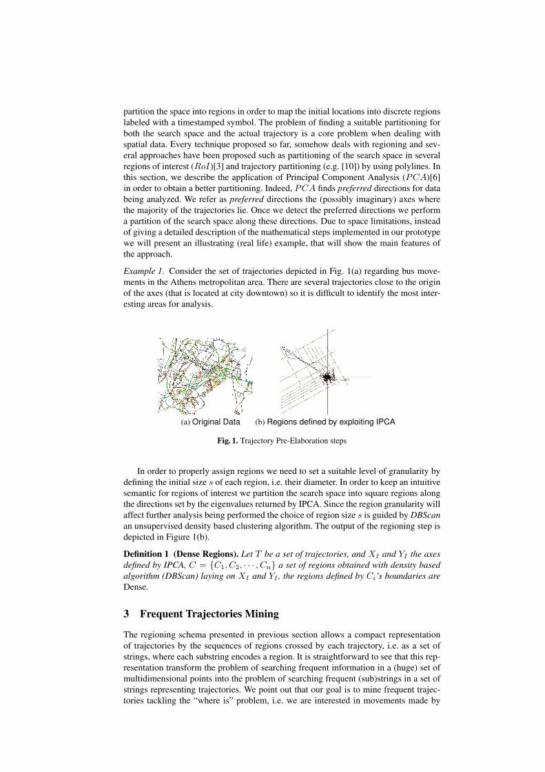
Example 1. Consider the set of trajectories depicted in Fig. 1(a) regarding bus move-ments in the Athens metropolitan area. There are several trajectories close to the originof the axes (that is located at city downtown) so it is difficult to identify the most inter-esting areas for analysis.

(a) Original Data (b) Regions defined by exploiting IPCA

Fig. 1. Trajectory Pre-Elaboration steps

In order to properly assign regions we need to set a suitable level of granularity bydefining the initial size s of each region, i.e. their diameter. In order to keep an intuitivesemantic for regions of interest we partition the search space into square regions alongthe directions set by the eigenvalues returned by IPCA. Since the region granularity willaffect further analysis being performed the choice of region size s is guided by DBScanan unsupervised density based clustering algorithm. The output of the regioning step isdepicted in Figure 1(b).

Definition 1 (Dense Regions). Let T be a set of trajectories, and XI and YI the axesdefined by IPCA, C = {C1, C2, · · · , Cn} a set of regions obtained with density basedalgorithm (DBScan) laying on XI and YI , the regions defined by Ci’s boundaries areDense.

3 Frequent Trajectories Mining

The regioning schema presented in previous section allows a compact representationof trajectories by the sequences of regions crossed by each trajectory, i.e. as a set ofstrings, where each substring encodes a region. It is straightforward to see that this rep-resentation transform the problem of searching frequent information in a (huge) set ofmultidimensional points into the problem of searching frequent (sub)strings in a set ofstrings representing trajectories. We point out that our goal is to mine frequent trajec-tories tackling the “where is” problem, i.e. we are interested in movements made by

objects disregarding time information (such as velocity). Moreover, since the numberof trajectories that could be monitored in real-life scenarios is really huge we needto work on successive portion of the incoming stream of data called windows. LetT = {T1, · · · , Tn} be the set of regioned trajectories to be mined belonging to thecurrent window; T contains several trajectories where each trajectory is a sequence ofregions. Let S = {S1, · · · , Sn} denotes the set of all possible (sub)trajectories of T . Thefrequency of a (sub)trajectory Si is the number of trajectories in T that contain Si, andis denoted as Count(Si, T ). The support of Si, sup(Si, T ), is defined as its frequencydivided by the total number of trajectories in T. Therefore, 0 ≤ sup(Si, T ) ≤ 1 foreach Si. The goal of frequent trajectories mining is to find all such Si, whose support isgreater than (or equal to) some given minimum support threshold α. The set of frequenttrajectories in T is denoted as Fα(T ). We consider in this paper frequent trajectoriesmining over a data stream, thus T is defined as a sliding window over the continuousstream. Each window either contains the same number of trajectories (count based orphysical window), or contains all trajectories arrived in the same period of time (time-based or logical window). T moves forward by a certain amount by adding the newslide (δ+) and dropping the expired one (δ−). Therefore, the successive instances of Tare shown as W1,W2, · · · . The number of trajectories that are added to (and removedfrom) each window is called its slide size. In this paper, for the purpose of simplicity,we assume that all slides have the same size, and also each window consists of the samenumber of slides. Thus, n = |W |/|S| is the number of slides (a.k.a. panes) in eachwindow, where |W | denotes the window size and |S| denotes the size of the slides.

Mining trajectories in W. As we obtain the string representation of trajectories, wefocus on the string mining problem. In particular, given a set of input strings, we wantto extract the (unknown) strings that obey certain frequency constraints. The frequentstring mining problem can be formalized as follows. Given a set T of input strings agiven frequency threshold α , find the set SF s.t. ∀s ∈ SF , count(s, T ) > α

Many proposal have been made to tackle this problem [7, 2]. We exploit in thispaper the approach presented in [7]. The algorithm works by searching for frequentstrings in different databases of strings, in our paper we do not have different databases,we have different windows instead. We first briefly recall the basic notions needed forthe algorithm, more details can be found in [7, 2].

The suffix array SA of a string s is an array of integers in the range [1.. n], whichdescribes the lexicographic order of the n suffixes of s. The suffix array can be com-puted in linear time [7]. In addition to the suffix array, we define the inverse suffix arraySA−1, which is defined by SA−1[SA[i]] = i ∀1 ≤ i ≤ n. The LCP table is an arrayof integers which is defined relative to the suffix array of a string s. It stores the lengthof the longest common prefix of two adjacent suffixes in the lexicographically orderedlist of suffixes. The LCP table can be calculated in O(n) from the suffix array and theinverse suffix array. The ω-interval is the longest common prefix of the suffixes is s.The algorithm is reported in Figure 2 and its features can be summarized as follows.

Function extractStrings arrange the the input strings in the window Wi in a stringSaux consisting of the concatenation of the strings in Wi, using # as a separation sym-bol and $ as termination symbol. Functions buildSuffixes and buildPrefixes computesrespectively the suffixes and prefixes of Saux and store them using SA and LCP vari-ables. Function computeRelevantStrings first compute the number of times that a strings occurs in Wi and then subtract so called correction terms which take care of multipleoccurrences within the same string of Wi as defined in [7]. The output frequent stringsare arranged in a tree structure that will be exploited for incremental mining purposesas will be explained in next section.

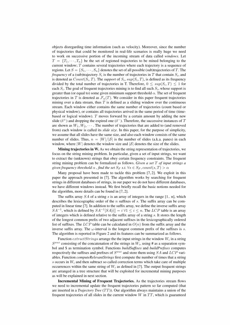
Incremental Mining of Frequent Trajectories. As the trajectories stream flowswe need to incremental update the frequent trajectories pattern so far computed (thatare inserted in a Trajectory Tree (TT )). Our algorithm always maintains a union of thefrequent trajectories of all slides in the current window W in TT , which is guaranteed

Method: MineFrequentStringsInput: A window slide S of the input trajectories;Output: A set of frequent strings SF .Vars:A string Saux;A suffix array SA;A prefix array LCP .1: Saux = extractStrings(S);2: SA = buildSuffixes(Saux);3: LCP = buildPrefixes(Saux);4: SF = computeRelevantStings(W0, SA,LCP )5: return SF ;

Fig. 2. The frequent string mining algorithm

to be a superset of the frequent pattern over W . Upon arrival of a new slide and expi-ration of an old one, we update the true count of each pattern in TT , by considering itsfrequency in both the expired slide and the new slide. To assure that TT contains allpatterns that are frequent in at least one of the slides of the current window, we mustalso mine the new slide and add its frequent patterns to TT . The difficulty is that whena new pattern is added to TT for the first time, its true frequency in the whole windowis not known, since this pattern wasn’t frequent in the previous n− 1 slides. To addressthis problem, we uses an auxiliary array (aux) for each new pattern in the new slide.The aux array stores the frequency of a pattern in each window starting at a particularslide in the current window. In other words, the auxiliary array stores frequency of apattern for each window, for which the frequency is not known. The key point is thatthis counting can either be done eagerly (i.e., immediately) or lazily. Under the laziestapproach, we wait until a slide expires and then compute the frequency of such new pat-terns over this slide and update the aux arrays accordingly. This saves many additionalpasses through the window. The pseudo code for the the algorithm is given in Figure 3.At the end of each slide, it outputs all patterns in TT whose frequency at that time is≥ αn|S|. However we may miss a few patterns due to lack of knowledge at the timeof output, but we will report them as delayed when other slides expire. The algorithmstarts when the first slide has been mined and its frequent trajectories are stored in TT .

Herein, function updateFrequencies updates the frequencies of each pattern inTT if it is present in S. As the new frequent patterns are mined (and stored in TT ′), weneed to annotate the current slide for each pattern as follows: if a given pattern t alreadyexisted in TT we annotate S as the last slide in which t is frequent, otherwise (t is a newpattern) we annotate S as the first slide in which t is frequent and create auxiliary arrayfor t and start monitoring it. When a slide expires (denote it Sexp) we need to update thefrequencies and the auxiliary arrays of patterns belonging to TT if they were presentin Sexp. Finally, we delete auxiliary array if pattern t has existed since arrival of S anddelete t, if t is no longer frequent in any of the current slides.

Algorithm Properties

Correctness This follows immediately from the fact that a pattern t belongs to Fα(W )(the frequent patterns is a window), only if it also belongs to ∩iFα(Si) (the union offrequent patterns for each slide i in the window). Thus, every frequent pattern in Wmust show up after mining of at least one of the slides and then we add it to TT .

Max Delay The maximum delay allowed by our algorithm is (n − 1) slides. Indeed,after expiration of (n − 1) slides, we will have a complete history of the frequency ofall frequent patterns of W and can report them. Moreover, the case in which a patternis reported after (n − 1) slides of time, is rare. For this to happen, patterns support in

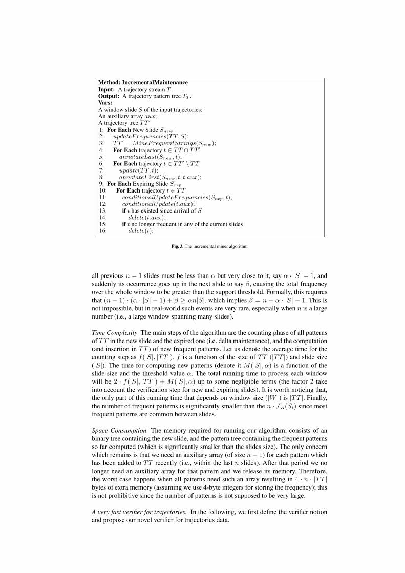
Method: IncrementalMaintenanceInput: A trajectory stream T .Output: A trajectory pattern tree TT .Vars:A window slide S of the input trajectories;An auxiliary array aux;A trajectory tree TT ′

1: For Each New Slide Snew

2: updateFrequencies(TT, S);3: TT ′ = MineFrequentStrings(Snew);4: For Each trajectory t ∈ TT ∩ TT ′

5: annotateLast(Snew, t);6: For Each trajectory t ∈ TT ′ \ TT7: update(TT, t);8: annotateF irst(Snew, t, t.aux);9: For Each Expiring Slide Sexp

10: For Each trajectory t ∈ TT11: conditionalUpdateFrequencies(Sexp, t);12: conditionalUpdate(t.aux);13: if t has existed since arrival of S14: delete(t.aux);15: if t no longer frequent in any of the current slides16: delete(t);

Fig. 3. The incremental miner algorithm

all previous n − 1 slides must be less than α but very close to it, say α · |S| − 1, andsuddenly its occurrence goes up in the next slide to say β, causing the total frequencyover the whole window to be greater than the support threshold. Formally, this requiresthat (n − 1) · (α · |S| − 1) + β ≥ αn|S|, which implies β = n + α · |S| − 1. This isnot impossible, but in real-world such events are very rare, especially when n is a largenumber (i.e., a large window spanning many slides).

Time Complexity The main steps of the algorithm are the counting phase of all patternsof TT in the new slide and the expired one (i.e. delta maintenance), and the computation(and insertion in TT ) of new frequent patterns. Let us denote the average time for thecounting step as f(|S|, |TT |). f is a function of the size of TT (|TT |) and slide size(|S|). The time for computing new patterns (denote it M(|S|, α) is a function of theslide size and the threshold value α. The total running time to process each windowwill be 2 · f(|S|, |TT |) + M(|S|, α) up to some negligible terms (the factor 2 takeinto account the verification step for new and expiring slides). It is worth noticing that,the only part of this running time that depends on window size (|W |) is |TT |. Finally,the number of frequent patterns is significantly smaller than the n · Fα(Si) since mostfrequent patterns are common between slides.

Space Consumption The memory required for running our algorithm, consists of anbinary tree containing the new slide, and the pattern tree containing the frequent patternsso far computed (which is significantly smaller than the slides size). The only concernwhich remains is that we need an auxiliary array (of size n− 1) for each pattern whichhas been added to TT recently (i.e., within the last n slides). After that period we nolonger need an auxiliary array for that pattern and we release its memory. Therefore,the worst case happens when all patterns need such an array resulting in 4 · n · |TT |bytes of extra memory (assuming we use 4-byte integers for storing the frequency); thisis not prohibitive since the number of patterns is not supposed to be very large.

A very fast verifier for trajectories. In the following, we first define the verifier notionand propose our novel verifier for trajectories data.

Definition 2. Let T be a trajectories database, P be a given set of arbitrary patternsand minfreq a given minimum frequency. A function f is called a verifier if it takesT , P and minfreq as input and for each pattern p ∈ P returns one of the followingresults: a) p’s true frequency in T if it has occurred at least minfreq times or otherwise;b) reports that it has occurred less than minfreq times (frequency not required in thiscase).

It is important to notice the subtle difference between verification and simple count-ing. In the special case of minfreq = 0 a verifier simply counts the frequency of allp ∈ P , but in general if minfreq > 0, the verifier can skip any pattern whose frequencywill be less than min freq. This early pruning can be done by the Apriori property orby visiting more than |T | −minfreq trajectories. Also, note that verification is differ-ent (and weaker) from mining. In mining the goal is to find all those patterns whosefrequency is at least minfreq, but verification simply verifies counts for a given set ofpatterns, i.e. verification does not discover additional patterns. Therefore, we can con-sider verification as a concept more general than counting, and different from (weakerthan) mining. The challenge is to find a verification algorithm, which is faster than bothmining and counting algorithms, since the algorithm for extracting frequent trajectorieswill benefit from this efficiency. In our case the verifier needs to take into account thesequential nature of trajectories so we need to count really fast while keeping the rightorder for the regions being verified. To this end we exploit an encoding scheme forregioned trajectories based on some peculiar features of prime numbers.

4 Encoding Paths for Efficient Counting and Querying

A great problem with trajectory sequential pattern mining is to control the exponen-tial explosion of candidate trajectory paths to be modeled because keeping informationabout ordering is crucial. Indeed, our regioning step heavily reduce the dataset size sothe number of regions we have to deal with is of hundreds of regions instead of thou-sands of points. Since our approach is stream oriented we also need to be fast whilecounting trajectories and (sub)paths. To this end, prime numbers exhibit really nice fea-tures that for our goal can be summarized in the following two theorems. They havealso been exploited for similar purposes for RFID tag encodings [8], but in that workthe authors did not provide a solution for paths containing cycles as we do in our frame-work.

Theorem 1 (The Unique Factorization Theorem). Any natural number greater than1 is uniquely expressed by the product of prime numbers.

As an example consider the trajectory T1 = ABC crossing three regions A,B,C.We can assign to regions A, B and C respectively the prime numbers 3,5,7 and theposition of A will be the first (pos(A) = 1), the position of B will be the second(pos(B) = 2), and the position of C will be the third (pos(C) = 3). Thus the resultingvalue for T1 (in the following we refer to it as P1) is the product of the three primenumbers, P1 = 3 ∗ 5 ∗ 7 = 105 that has the property that does not exist the product ofany other three prime numbers that gives as results 105.

As it is easy to see this solution allows to easily manage trajectories since contain-ment and frequency count can be done efficiently by simple mathematical operations.Anyway, this solution does not allow to distinguish among ABC, ACB, BAC, BCA,CAB, CBA, since the trajectory number (i.e. the product result) for these trajectoriesis always 105. To this end we can exploit another fundamental theorem of arithmetics.

Theorem 2 (Chinese Remainder Theorem). Suppose that n1, n2, · · · , nk are pair-wise relatively prime numbers. Then, there exists W (we refer to it as witness) between0 and N = n1·n2 · · ·nk solving the system of simultaneous congruences: W%n1 = a1,W%n2 = a2, . . ., W%nk = ak.

Then, by Theorem 2, there exists W1 between 0 and P1 = 3 ∗ 5 ∗ 7 = 105. In ourexample, the witness W1 is 52 since 52%3 = 1 = pos(A) and 52%5 = 2 = pos(B)and 52%7 = 3 = pos(C). We can compute W1 efficiently using the extended Euclideanalgorithm. From the above properties it follows that in order to fully encode a trajectory(i.e. keeping the region sequence) it suffices to store two numbers its prime numberproduct (we refer to it as trajectory number) and its witness. As a nice side-effect inorder to obtain any information about region positions in the trajectory we can testwith the maximum efficiency containment relationships (a simple division) and orderchecking (a sequence of divisions). In order to assure that no problem will arise in theencoding phase and witness computation we assume that the first prime number wechoose for encoding is greater than the trajectory size. So for example if the trajectorylength is 3 we encode it using prime numbers 5,7,11. A devil’s advocate may argue thatmultiple occurrences of the same region leading to cycles violate the injectivity of theencoding function. To this end the following example will clarify our strategy.

Dealing with cycles. Consider the following trajectory T2 = ABCAD, we havea problem while encoding region A since it appears twice in the first and fourth posi-tion. We need to assure that the encoding value of A is such that we can say that bothpos(A) = 1 and pos(A) = 4 hold(we do not want two separate encoding value sincethe region is the same and we are interested in the order difference). Assume that Ais encoded as (41)5 (i.e. 41 on base 5, we use 5 base since the trajectory length is 5))this means that A occurs in positions 1 and 4. The decimal number associated to it isA = 21, and we chose as the encoding for A = 23 that is the first prime number greaterthan 21. Now we encode the trajectory using A = 23, B = 7, C = 11, D = 13 thusobtaining P2 = 23023 and W2 = 2137 (since the remainder we need for A is 21). As iteasy to see we are still able to properly encode even trajectories containing cycles. Asa final notice we point out that the above calculation is made really fast by exploiting aparallel algorithm for multiplication operation. We do not report here the pseudo codefor the encoding step explained above due to space limitations. Finally, one may arguethat the size of prime numbers could be large, however in our case it is bounded sincethe number of regions is small as confirmed by several empirical studies [5](always lessthan a hundred of regions for real life applications we investigated).

Definition 3 (Region Encoding). Given a set R = {R1, R2, · · · , Rn} of regions, afunction enc from R to P (the positive prime numbers domain) is a region encodingfunction for R.

Definition 4 (Trajectory Encoding). Let Ti = R1, R2 · · ·Rn be a regioned trajectory.A trajectory encoding (E(Ti)) is a function that associates Ti with a pair of integernumbers ⟨Pi,Wi⟩ where Pi =

∏1..n enc(Ri) is the trajectory number and Wi is the

witness for Pi.

Once we encode each trajectory as a pair E(T ) we can store trajectories in a binarysearch tree making the search, update and verification operations quite efficient sinceat each node we store the E(T ) pair. It could happen that there exists more than onetrajectory encoded with the same value P but different witnesses. In this case, we storeonce the P value and the list of witnesses saving space for pointers and for the duplicateP ’s value. Consider the following set of trajectories along with their encoding values(we used region encoding values: A = 5, B = 7, C = 11, D = 13, E = 15): (ABC,⟨385, 366⟩), (ACB, ⟨385, 101⟩), (BCDE, ⟨15015, 3214⟩), (DEC, ⟨2145, 872⟩). ABCand ACB will have the same P value (385) but their witnesses are W1 = 366 andW2 = 101, so we are still able to distinguish them.

Claim. The proposed trajectory encoding scheme performs a one-to-one encoding forany trajectory.

The proof easily follows by Theorem 2 by injectivity of prime numbers conversionproperties.

Method: checkContainmentInput:Two trajectories encodings E(T1) and E(T2);Output:Yes if T1 ∈ T2, no otherwise;Method:1: if P1 > P2 return NO2: if P2%P1 = 0 then3: for each R1

i

4: if pos((next(R1i ))

2) < pos(R2i ) return NO

5: return YES

Method: updateTreeInput:a trajectory tree BT and a new window NEW ;Output:the updated version of BT ;Vars:a tree node N ;Method:1: for each Ti ∈ NEW2: N = depthSearch(E(Ti))3: if N = null4: BT = updateFrequency(N,E(Ti))5: else insertNode(E(Ti))6: if memoryneeded deleteOlderNode(BT )7: return BT

Fig. 4. Algorithms for checking containment and update tree

Once computed the encoded trajectories we build our synopsis by storing them ina search binary tree associated to the input trajectories. At each node of the binary treewe store the trajectory number, the witness and the frequency count for each trajectory.The insertion, remove and update operations have the usual meaning.

A simple algorithm for checking ordered containment. In order to perform ef-ficient trajectory verification we should be able to check containment relationships be-tween trajectories. More in detail, given two trajectories, we call them T1 and T2, andtheir encodings E(T1) and E(T2) we need to answer this question ‘Is T1 a sub-sequenceof T2?’. To this end we can exploit the mathematical features of encoded trajectoriesto design a simple and effective algorithm. In the following we denote the index of aregion Ri ∈ Ti as pos(Ri) and the region following Ri in Ti as next(Ri), we recallthat we do not need to store the region positions since they can be obtained by simplemath calculation on witnesses. If a region Ri appears into two different trajectories Tl

and Tm we denote it as Rli and Rm

i .The algorithm first checks if P value of T1 is a divider of P value of T2, if the

latter holds this means that all the regions belonging to T1 also belongs to T2. To testif containment holds we need to check that every pair of consecutive regions in T1 arealso consecutive in T2. Consider again our toy example and suppose to check wetherT1 = BC is contained in T2 = ABC. we have that P2 = 385 and P1 = 77. We testthat P2%P1 = 0, now we have that pos(B2) = 2 < 3 = pos(C2) thus the answer tothe containment test is Y ES. In order to build a fast verifier for trajectory frequencies,we store an additional information at each node, i.e. the frequency of the trajectoriesstored at that node. Obviously if we have more than one witness for a given P valuewe will store the frequencies for each witness. Again, doing this we prevent new nodesinsertion thus saving memory space. The initial tree is built for the first window W1,we call it BT . As new trajectories arise in the stream we continuously update it. Inparticular, for every incoming trajectory Ti ∈ NEW we search the node N it belongsto by performing a depthSearch on BT of the encoding values for T (E(Ti)). If such anode N exists (this means that Ti is frequent) we update its frequency. In particular weupdate the frequency of the witness Wi for Ti (we recall that there may exists more thanone witness for the same P value). If the trajectory does not exist in the tree we insertthe corresponding node (annotating its timestamp). Finally, as the stream flows if weneed to release memory we delete the older nodes (i.e. the ones with older timestamps).

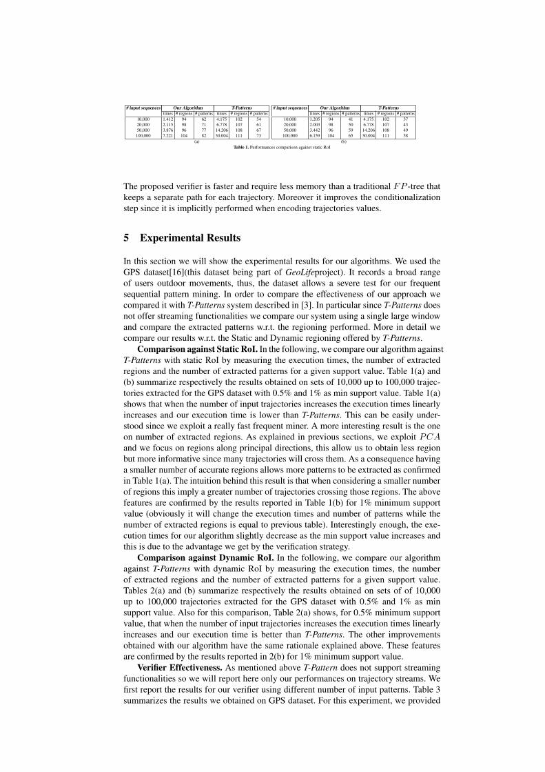
# input sequences Our Algorithm T-Patternstimes # regions # patterns times # regions # patterns

10,000 1.412 94 62 4.175 102 5420,000 2.115 98 71 6.778 107 6150,000 3.876 96 77 14.206 108 67

100,000 7.221 104 82 30.004 111 73


10,000 1.205 94 41 4.175 102 3720,000 2.003 98 50 6.778 107 4350,000 3.442 96 59 14.206 108 49

100,000 6.159 104 65 30.004 111 58(a) (b)

Table 1. Performances comparison against static RoI

The proposed verifier is faster and require less memory than a traditional FP -tree thatkeeps a separate path for each trajectory. Moreover it improves the conditionalizationstep since it is implicitly performed when encoding trajectories values.

5 Experimental Results

In this section we will show the experimental results for our algorithms. We used theGPS dataset[16](this dataset being part of GeoLifeproject). It records a broad rangeof users outdoor movements, thus, the dataset allows a severe test for our frequentsequential pattern mining. In order to compare the effectiveness of our approach wecompared it with T-Patterns system described in [3]. In particular since T-Patterns doesnot offer streaming functionalities we compare our system using a single large windowand compare the extracted patterns w.r.t. the regioning performed. More in detail wecompare our results w.r.t. the Static and Dynamic regioning offered by T-Patterns.

Comparison against Static RoI. In the following, we compare our algorithm againstT-Patterns with static RoI by measuring the execution times, the number of extractedregions and the number of extracted patterns for a given support value. Table 1(a) and(b) summarize respectively the results obtained on sets of 10,000 up to 100,000 trajec-tories extracted for the GPS dataset with 0.5% and 1% as min support value. Table 1(a)shows that when the number of input trajectories increases the execution times linearlyincreases and our execution time is lower than T-Patterns. This can be easily under-stood since we exploit a really fast frequent miner. A more interesting result is the oneon number of extracted regions. As explained in previous sections, we exploit PCAand we focus on regions along principal directions, this allow us to obtain less regionbut more informative since many trajectories will cross them. As a consequence havinga smaller number of accurate regions allows more patterns to be extracted as confirmedin Table 1(a). The intuition behind this result is that when considering a smaller numberof regions this imply a greater number of trajectories crossing those regions. The abovefeatures are confirmed by the results reported in Table 1(b) for 1% minimum supportvalue (obviously it will change the execution times and number of patterns while thenumber of extracted regions is equal to previous table). Interestingly enough, the exe-cution times for our algorithm slightly decrease as the min support value increases andthis is due to the advantage we get by the verification strategy.

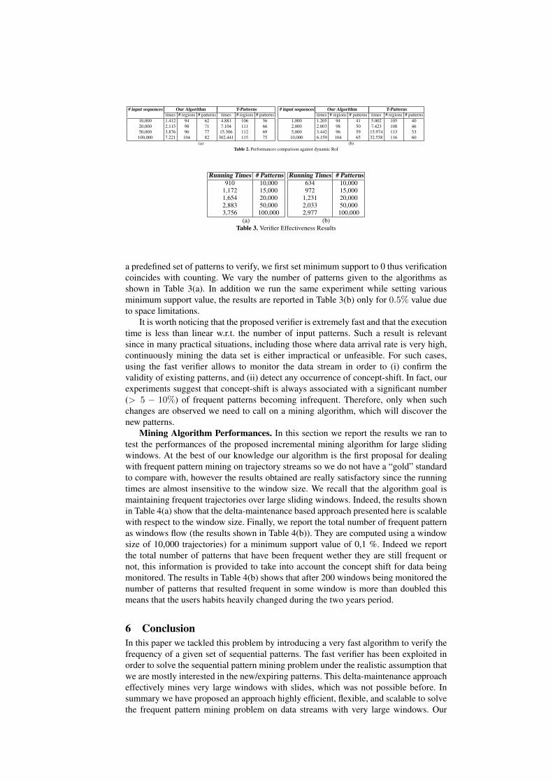
Comparison against Dynamic RoI. In the following, we compare our algorithmagainst T-Patterns with dynamic RoI by measuring the execution times, the numberof extracted regions and the number of extracted patterns for a given support value.Tables 2(a) and (b) summarize respectively the results obtained on sets of of 10,000up to 100,000 trajectories extracted for the GPS dataset with 0.5% and 1% as minsupport value. Also for this comparison, Table 2(a) shows, for 0.5% minimum supportvalue, that when the number of input trajectories increases the execution times linearlyincreases and our execution time is better than T-Patterns. The other improvementsobtained with our algorithm have the same rationale explained above. These featuresare confirmed by the results reported in 2(b) for 1% minimum support value.

Verifier Effectiveness. As mentioned above T-Pattern does not support streamingfunctionalities so we will report here only our performances on trajectory streams. Wefirst report the results for our verifier using different number of input patterns. Table 3summarizes the results we obtained on GPS dataset. For this experiment, we provided


10,000 1.412 94 62 4.881 106 5620,000 2.115 98 71 7.104 111 6650,000 3.876 96 77 15.306 112 69

100,000 7.221 104 82 302.441 115 75


1,000 1.205 94 41 5.002 105 402,000 2.003 98 50 7.423 108 465,000 3.442 96 59 15.974 113 53

10,000 6.159 104 65 32.558 116 60(a) (b)

Table 2. Performances comparison against dynamic RoI

Running Times # Patterns910 10,000

1,172 15,0001,654 20,0002,883 50,0003,756 100,000

Running Times # Patterns634 10,000972 15,000

1,231 20,0002,033 50,0002,977 100,000

(a) (b)Table 3. Verifier Effectiveness Results

a predefined set of patterns to verify, we first set minimum support to 0 thus verificationcoincides with counting. We vary the number of patterns given to the algorithms asshown in Table 3(a). In addition we run the same experiment while setting variousminimum support value, the results are reported in Table 3(b) only for 0.5% value dueto space limitations.

It is worth noticing that the proposed verifier is extremely fast and that the executiontime is less than linear w.r.t. the number of input patterns. Such a result is relevantsince in many practical situations, including those where data arrival rate is very high,continuously mining the data set is either impractical or unfeasible. For such cases,using the fast verifier allows to monitor the data stream in order to (i) confirm thevalidity of existing patterns, and (ii) detect any occurrence of concept-shift. In fact, ourexperiments suggest that concept-shift is always associated with a significant number(> 5 − 10%) of frequent patterns becoming infrequent. Therefore, only when suchchanges are observed we need to call on a mining algorithm, which will discover thenew patterns.

Mining Algorithm Performances. In this section we report the results we ran totest the performances of the proposed incremental mining algorithm for large slidingwindows. At the best of our knowledge our algorithm is the first proposal for dealingwith frequent pattern mining on trajectory streams so we do not have a “gold” standardto compare with, however the results obtained are really satisfactory since the runningtimes are almost insensitive to the window size. We recall that the algorithm goal ismaintaining frequent trajectories over large sliding windows. Indeed, the results shownin Table 4(a) show that the delta-maintenance based approach presented here is scalablewith respect to the window size. Finally, we report the total number of frequent patternas windows flow (the results shown in Table 4(b)). They are computed using a windowsize of 10,000 trajectories) for a minimum support value of 0,1 %. Indeed we reportthe total number of patterns that have been frequent wether they are still frequent ornot, this information is provided to take into account the concept shift for data beingmonitored. The results in Table 4(b) shows that after 200 windows being monitored thenumber of patterns that resulted frequent in some window is more than doubled thismeans that the users habits heavily changed during the two years period.

6 ConclusionIn this paper we tackled this problem by introducing a very fast algorithm to verify thefrequency of a given set of sequential patterns. The fast verifier has been exploited inorder to solve the sequential pattern mining problem under the realistic assumption thatwe are mostly interested in the new/expiring patterns. This delta-maintenance approacheffectively mines very large windows with slides, which was not possible before. Insummary we have proposed an approach highly efficient, flexible, and scalable to solvethe frequent pattern mining problem on data streams with very large windows. Our

Running Times Windows size773 10,000891 25,000

1,032 50,0001,211 100,0001,304 500,0002,165 1,000,000

# Window # Patterns1 8510 10620 12550 156100 189200 204

(a) (b)Table 4. Mining Algorithm Results

work is subject to further improvements in particular we will investigate: 1) furtherimprovements to the regioning strategy; 2) refining the incremental maintenance to dealwith maximum tolerance for delays between slides.

7 Acknowledgments

The authors would like to thank Barzan Mozafari for the invaluable discussions thatoriginated this work.

References

1. R. Agrawal and R. Srikant. Fast algorithms for mining association rules in large databases.In VLDB, 1994.

2. Johannes Fischer, Volker Heun, and Stefan Kramer. Optimal string mining under frequencyconstraints. In PKDD, pages 139–150, 2006.

3. Fosca Giannotti, Mirco Nanni, Fabio Pinelli, and Dino Pedreschi. Trajectory pattern mining.In KDD, pages 330–339, 2007.

4. J. Han, J. Pei, and Y. Yin. Mining frequent patterns without candidate generation. In SIG-MOD, 2000.

5. H. Jeung, M. Lung Yiu, X. Zhou, C. S. Jensen, and H. T. Shen. Discovery of convoys intrajectory databases. PVLDB, 1(1):1068–1080, 2008.

6. I.T. Jolliffe. Principal Component Analysis. Springer Series in Statistics, 2002.7. A. Kugel and E. Ohlebusch. A space efficient solution to the frequent string mining problem

for many databases. Data Min. Knowl. Discov., 17(1):24–38, 2008.8. C-H Lee and C-W Chung. Efficient storage scheme and query processing for supply chain

management using rfid. In SIGMOD08, pages 291–302, 2008.9. J-G Lee, J. Han, X. Li, and H. Gonzalez. TraClass: trajectory classification using hierarchical

region-based and trajectory-based clustering. PVLDB, 1(1):1081–1094, 2008.10. J-G Lee, J. Han, and K-Y Whang. Trajectory clustering: a partition-and-group framework.

In SIGMOD07, pages 593–604, 2007.11. J. Li, D. Maier, K. Tufte, V. Papadimos, and P. A. Tucker. No pane, no gain: efficient evalu-

ation of sliding-window aggregates over data streams. SIGMOD Rec., 34(1):39–44, 2005.12. Y. Liu, L. Chen ., J. Pei, Q. Chen, and Y. Zhao. Mining frequent trajectory patterns for

activity monitoring using radio frequency tag arrays. In PerCom, pages 37–46, 2007.13. E. Masciari. Trajectory clustering via effective partitioning. In FQAS, pages 358–370, 2009.14. Elio Masciari. Warehousing and querying trajectory data streams with error estimation. In

DOLAP, pages 113–120, 2012.15. B. Mozafari, H. Thakkar, and C. Zaniolo. Verifying and mining frequent patterns from large

windows over data streams. In ICDE, pages 179–188, 2008.16. Y. Zheng, Q. Li, Y. Chen, and X. Xie. Understanding mobility based on gps data. In Ubi-

Comp 2008, pages 312–321, 2008.

Documents

Sequential Pattern Mining from Trajectory Data