Embed Size (px)
Citation preview
1
SEQUENTIAL METHODS IN PARAMETER ESTIMATIONJames V. Beck, Professor Emeritus, Dept. Of Mech. Eng., Michigan State Univ., East Lansing, MI 48864, e-mail: [email protected]
ABSTRACT
A tutorial is presented of the subject of parameter estimation with particular reference to examples in heat transfer. Parameter estimationis differentiated from function estimation, which is closely related . Parameter estimation is presented as one dealing with experiments and analysiswith a relatively small number of parameters and as a consequence is usually not ill-posed. In contrast, function estimation usually has a largenumber of parameters and usually is ill-posed. Both linear and nonlinear estimation are covered. Of particular emphasis is the concept ofsequential estimation in a particular experiment (adding one measurement after another) and over experiments (using prior information).Sequential analysis does provide a means to treat some aspects of ill-posed problems and is related to Tikhonov regularization. Sequentialparameter estimation also helps to provide insights in the adequacy of the mathematical models and accuracy of the parameter estimates. Confidence intervals and regions are investigated, including the conservative Bonferroni method. A Monte Carlo study is given to demonstratethe validity of the confidence regions. Sensitivity coefficients are shown to appear in the estimation of parameters, determination of confidenceregions and design of optimal experiments.
1. INTRODUCTION
The purpose of this paper is to summarize some parameter estimation concepts. Some of these may be colored by applications in
experimental heat transfer. Parameter estimation provides an analytical means of estimating constants in mathematical models given appropriate
measurements, building mathematical models and giving insight into the design of experiments. Both linear and nonlinear estimation problems
exist, with the latter being much more important. However, the concepts are easier to understand for linear cases. Many of the points given herein
are expanded in Beck and Arnold (1).
In the past three decades many papers and books have been written about parameter estimation in engineering. The name “parameter
estimation” has not been universally used for the same process. Some other names, sometimes with slightly different connotations, are nonlinear
parameter estimation (Bard ( 2)), nonlinear estimation or regression (Seber and Wild (3); Ross (4)), identification , system identification
(Goodwin and Payne (5); Eykhoff (6); Ljung (7)), inverse problems (Alifanov (8); Alifanov, O.M., E.A. Artyukhin and S.V. Rumyantsev (9);
Trujillo and Busby (10); Hensel (11); Ozisik (12); Isakov (13); Tarantola (14); Kurpisz and Nowak (15)), data analysis or reduction (Bevington
(16)); Menke (17)), nonlinear least squares (Bjorck (18); Lawson and Hansen (19); Box and Draper (20)), mollification method (Murio (21)),
ill-posed problems(Beck, Blackwell and St. Clair (22); Murio (21); Tikhonov and Arsenin (23) and others. An engineering journal, Inverse
Problems in Engineering , is devoted partly to parameter estimation in engineering.
An outline of the remainder of this survey is now given. First, some distinctions between parameter and function estimation are given.
Then some common research paradigms in heat transfer are given. Next the main mathematical formalism starts with a development of sequential
estimation over experiments for linear problems. This topic leads to a brief discussion of ill-posed problems and Tikhonov regularization.
Nonlinear estimation starts with a matrix of the Taylor series expansion and then the Gauss method of minimization. The survey ends with an
introduction to confidence regions and mention of optimal experiments.
2. PARAMETER VS. FUNCTION ESTIMATION
Inverse problems can be divided into two classes: parameter estimation and function estimation. I have found that distinction to be
helpful and will describe why. The distinction is not always made, partly because many problems can be treated as function estimation problems
and thus include parameter estimation problems. In my mind parameter estimation has a somewhat different connotation than function estimation
in heat transfer.
I will preface some of these remarks with the observation is that I am speaking as an engineer. Mathematicians have a somewhat
different view as indicated by Prof. P.K. Lamm (24), “Mathematicians generally think of "function estimation" as the determination of an
infinite-dimensional function (not just a finite-dimensional discretization of a function, even though the dimension may be quite large). But this
is a theoretical concept, and when one goes to implement the theory, one typically resorts to finite-dimensional approximations. This
2
Nu
qLk(T(0)T
�
) (1)
finite-dimensional approximation should converge to the infinite-dimensional function that is being sought.”
Some aspects are now given which, if not unique to parameter estimation, are emphasized more than in function estimation.
1. A limited number of parameters are estimated. In heat transfer the number can be as small as one and might be as large as half a
dozen and on occasion could even go even higher.
2. The problems are usually not ill-posed but are usually nonlinear even if the describing differential equation is linear.
3. The parameters frequently refer to a physical property, such as thermal conductivity for a specified material at a particular
temperature. These properties are not subject to human adjustment, as for example, a heat flux function is.
4. Parameter estimation analysis is not complete without giving an estimate of the confidence interval or region.
5. Model-building is an important part of parameter estimation; that is, we have a physical process that we may not understand and we
wish to model it more perfectly.
6. Careful examination of residuals (measured values minus estimated values of measured variables) is done to check the adequacy of
the mathematical model and to understand the measurement errors more fully. The residuals should not have a characteristic signature that persists
experiment after experiment. Such a characteristic signature indicates a bias which affects the parameter estimates. This bias may give insight
into improvements in the model (model-building). If the bias cannot be removed, it is desirable to quantify the effects of this bias.
7. The chosen sum of squares or weighted sum of squares function should be selected based upon the measurement errors.
8. A powerful way to investigate the adequacy of the model and experiment is to estimate the parameters sequentially. These parameter
estimates should approach constant values rather than drifting upward or downward at the end of the analysis interval.
9. Optimal experiment design is very important in obtaining the best accuracy of the estimates.
10. Insight is of primary concern while computational efficiency may not be.
In contrast to parameter estimation, function estimation usually has the following characteristics.
1. The number of parameters to describe a function is usually large, maybe in the hundreds or even thousands.
2. The problems are usually ill-posed and might or might not be linear.
3. Computational efficiency is important. This may lead to avoiding calculation of the sensitivity coefficients. Insight into the
sensitivity of various components is not usually of interest.
4. Confidence intervals, model building, residual analysis, optimal experiment design, statistics, and sequential parameter estimates
are rarely considered.
3. COMMON RESEARCH PARADIGMS IN HEAT TRANSFER
Two types of paradigms, denoted A and B, in heat transfer research are commonly used. In these paradigms the emphasis is upon the
analytical operations for estimating the parameters or modeling a process . The paradigms may be used independently or simultaneously. A third
and less commonly used paradigm, Paradigm C, exploits the concepts of inverse problems including parameter and function estimation. This
paradigm has greater power for modeling and estimating parameters in heat transfer phenomena.
Although the two common research paradigms do not include all approaches, the distinctions help to provide insight. Paradigm A
involves determining a single unknown. Paradigm B has the objective of verifying that a proposed mathematical model is satisfactory.
In Paradigm A, the experiment may or may not be complex. In fact, experimental complexity might be needed to simplify the analysis.
The essence of this paradigm is that the analytical model for determining the unknown parameter is a simple algebraic expression for estimating
a single parameter. For the Nusselt number, Nu, being the unknown parameter, the model might be
where q is the measured surface heat flux, T(0) is the measured surface temperature, k is the fluid conductivity and T�
is the measured fluid

3
temperature. Only one parameter is found for each experiment, such as finding the Nu value at a given Reynolds number (or fluid velocity).
In Paradigm A, the mathematical model is made as simple as possible in terms of the measurements. In some experiments, periodic
conditions are used to obtain solutions in terms of the amplitude and phase shift, which are simple functions of the desired parameters. Also some
experiments may be quasi-state to simplify the solution. A primary emphasis is upon developing and using a simple algebraic solution for a single
parameter. Examination of the validity of model is not usually a part of this paradigm because residuals are not available.
In Paradigm B, an incompletely understood heat transfer process is investigated in two distinct and complementary ways: one uses
experiments and the other uses analytical or computer modeling. An experimental group produces temperatures or other quantities measured
as a function of time or position. The experimental group then in effect throws the data “over the wall” together with a description of the
experiment to the analytical group. Without using these experimental data (but possibly using information from handbooks or independent
Paradigm A experiments), analysts build a mathematical model, which may be a differential equation (or set of equations) and appropriate
boundary conditions, source terms and initial conditions. Usually finite differences or finite elements are used to incorporate the model in a
computer program. Then a large computation is performed which includes relevant physics and mimics the experiment; finally, a graph of overall
results is produced. Characteristically, the comparison of the graphical results is just visual and not quantitative. Instead the agreement almost
always is simply said to be "satisfactory" or even "excellent", indicating that the model is also satisfactory. An important point is that the results
of the experiment and analysis are purposely kept apart until the last possible moment, and then compared only on the same plot. Usually the
results of the model are not used to modify or improve the experiment. Also the model may not be modified based on what is learned from the
experiment.
In Paradigm B the intent is to avoid any “knobs” to turn to get agreement between the model and the measurements. Such an approach
is appropriate in areas where the fundamental model is known. For cases when the solid or fluid changes undergoes transient and permanent
changes because of phase transformations in metals, combustion, ablation or curing, Paradigm B is frequently not powerful enough to determine
the appropriate model, parameters and/or functions.
Paradigm C utilizes the power of inverse problems. The emphasis is upon combined experiments and analysis. The paradigm is directed
toward understanding some physical heat transfer process which has some unknown aspects. Although the unknown aspects might be the
appropriate model (differential equations, initial and boundary conditions), it could also involve estimating several unknown parameters or even
a function. A fundamental difference between paradigms A and C are that in paradigm A the model is a simple algebraic one for a single
parameter while in paradigm C, the model can be complex involving the solution of partial differential equations and more than one unknown.
An example of unknown parameters is the estimation of temperature dependent thermal conductivity and volumetric heat capacity of a new
composite material from transient temperature measurements. In this case both properties might be modeled for a moderate temperature range
as a linear function of temperature, resulting in four parameters with two for each. In experiments even as simple this example, the design of
the experiment is important and can greatly influence the accuracy of the estimated parameters. This then means that the experiments should
be carefully designed; selection of the basic geometry (plate or radial), size of specimen, type and time variation of boundary conditions, types
of sensors (temperature and/or heat flux) and location of sensors are all important considerations.
4. SEQUENTIAL ESTIMATION OVER EXPERIMENTS FOR LINEAR PROBLEMS
It is customary for experimentalists to analyze each experiment separately for parameters, even though the same set of parameters is
being estimated or overlap exists between estimated parameters in subsequent experiments. Another approach is to analyze the data for all the
experiments at the same time. In a series of experiments, one experiment may be performed at given conditions and at a given time; others are
performed, possibly days or weeks later. For example, thermal diffusivity is found using the laser flash method. Several experiments for a given
material and temperature level might be performed and each experiment is analyzed separately for the thermal diffusivity. A better approach might
be to combine all the data to obtain the estimated diffusivity at that temperature. One can also simultaneously estimate for parameters describing
a temperature (or other) dependence.
Sequential estimation can be accomplished in the fairly straightforward approach described in this herein or using the more general
maximum a posteriori method, Beck and Arnold (1). An objective in this survey is to simplify the presentation by minimizing statistical
considerations, although they are important. Furthermore the beginning analysis considers the linear problem, which is linear because the model
4
X1
X11 X12 á X1p
X21 X22 á X2p
� � á �
Xn1 Xn2 á Xnp 1
(2)
y1��1���1 (3)
S1(y1X1��)TW1(y1X1��), S2(y2X2��)TW2(y2X2��) (4)
S1Mn
i1
yi (Xi1�1�Xi2�2�á�Xip� p)2
1 (5)
b i(XTi W iX i)
1XTi W iy i, i1, 2 (6)
is linear in terms of the parameters.
Suppose experiment 1 has been performed yielding the measurement vector y1 (dimensions of n × 1) for conditions which are described
by the sensitivity matrix X1. The subscript “1" denotes experiment 1. The matrix X1, which we shall call the sensitivity matrix, can be written
in detail as
This matrix has dimensions of n × p, where n is the number of measurements and p is the number of parameters. The corresponding model is
��1 = X1��, where �� is the parameter vector with p components; in general n is much larger than p. For the first experiment, the measurements and
the model are related by
where ��1 is the measurement error vector for experiment 1. Another experiment is performed and the measured vector is denoted y2 and the model
is ��2 = X2��. Notice that the same parameter vector is present for both experiments.
The criterion chosen to estimate the parameters depends upon the nature of the measurement errors. We can minimize a weighted sum
of squares function for each experiment separately,
The weighting matrices, W1 and W2, are selected based upon the statistical characteristics of the measurement errors. If these errors conform to
the statistical assumptions of having constant variance and being uncorrelated, the weighting matrices can be replaced by the identity matrix,
I, permitting the use of summation notation,
The 1 subscript on the far right denotes that the measurement vector y and the sensitivity matrix X are for experiment one.
It is not necessary that the experiments be similar. Different types of measurements can be obtained and different measurement devices
could be used in the two experiments. The weighting coefficients might be different, although both ideally should be related to the inverse of
the covariance matrix of the measurement errors (Beck and Arnold (1)). Also each experiment might have a different number of measurements,
n1 and n2 where n1 might be quite different from n2.
The conventional method of analysis is to estimate �� from each sum of squares function to get
5
S1,2S1��S2 (7)
b1,2(XTWX)1XTWy (8)
X
X1
X2
, W
W1 0
0 W2
, yy1
y2
(9)
b1,2(XT1 W1X1��XT
2 W2X2)1(XT
1 W1y1��XT2 W2y2) (10)
V11 XT
1 W1X1 (11)
Sb(y2X2��)TW2(y2X2��)��(b1��)TV11 (b1��) (12)
where bi is the estimated parameter vector for the ith experiment. (We pause here to point out that although an inverse is implied here, this
equation is displayed in this fashion only for our human understanding. The actual computations used in solving for the parameters rarely involve
inverses. If a program such as Matlab is used, the solution method has been optimized and we need not delve into it. We leave it to the numerical
analysts. However, we prefer the sequential method of solution which is given below.)
A common practice to find the best results for two experiments for estimating the same parameter vector is to use the average, (b1 +
b2)/2. If the two experiments are equivalent in measurement accuracy, that would be a reasonable procedure. If the two experiments had different
numbers of measurements or were intrinsically different, the simple average may not be appropriate.
Another estimation procedure is to estimate the parameters using all the data at once, that is, to minimize
The result is the estimator
where the components are
The extension of eq. (9) to m experiments is straightforward, simply having columns of m Xi and yi values and adding terms along the diagonal
of W. The 1,2 subscript in eq. (8) means that the data from experiments 1 and 2 are used. More explicitly eq. (8) can be written as
which can be extended in a direct manner to more experiments. (Again we point out that the presence of the inverse notation does not mean that
the numerical computation for the estimate will actually use the inverse operation.)
Another method of deriving eq. (10) is now considered. Let
and we minimize now the function
6
/��Sb2XT
2 W2(y2X2��)2V11 (b1��) (13)
(XT2 W2X2��V1
1 )bbXT2 W2y2��V1
1 b1 (14)
bb(XT2 W2X2��V1
1 )1(XT2 W2y2��V1
1 b1 ) (15)
bb(XT2 W2X2��XT
1 W1X1)1(XT
2 W2y2��XT1 W1X1b1 ) (16)
Si�1(yi�1Xi�1��)TWi�1(yi�1Xi�1��)��(b i��)TV1i (b i��) (17)
V1i XT
1 W1X1��XT2 W2X2���XT
i W iX i (18)
Take the matrix derivative of eq. (12) with respect to �� to get (Beck and Arnold (2), chap. 6)
Now replacing �� by bb and setting eq. (13) equal to 0 then gives
Eq. (14) can be re-written several ways. One is to solve directly for the estimator to get
Another way to write is to use the definition of V1 given by eq. (11) which yields
Using eq. (6) for i = 1 gives an expression for b1 that will reduce the right side of eq. (16) to exactly the same as the right side of eq. (10). Hence
bb is the same as b1,2. Consequently if one experiment has been analyzed to obtain its estimated parameter vector b1, the simultaneous analysis
of these two experiments together can be obtained by using eq. (15). Notice that eq. (15) requires only b1 and V1-1 = X1
TW1X1. These two
matrices contain all the needed information to combine the two experiments to obtain the new estimate. (More information might be needed to
calculate confidence intervals and regions.) It means that the n1 measurements from experiment 1 can be discarded if the new combined parameter
vector is the only one of interest.
One might extend the “sequential over experiments” concept to the analysis of many experiments, one combining the results of the
previous ones. In this analysis the notation will be changed from that above for b and S. Now let bi, Vi and Si be the values for all the experiments
simultaneously considered, rather than b1,2, ...,i, for example. However, yi+1, Wi+1 and Xi+1 refer just to the (i+1)st experiment as above. For
combining the results of the (i+1)st experiment with the previous 1, 2, . . ., i experiments, the sum of squares function is started with
where Vi-1 is given by
Taking the matrix derivative of eq. (17) with respect to ��, replacing �� with bi+1 and setting equal to 0 gives
7
2XTi�1Wi�1(yi�1Xi�1bi�1)2V1
i (b ibi�1)0 (19)
bi�1(XTi�1Wi�1Xi�1��V1
i )1(XTi�1Wi�1yi�1��V1
i b i ) (20a)
bi�1b i��(XTi�1Wi�1Xi�1��V1
i )1 XTi�1Wi�1(yi�1Xi�1b i ) (20b)
V1i V1
i1��XTi77 iX i (21)
Pi�1(P1i �XT
i�1wi�1Xi�1)1 (22)
Solving for bi+1 gives
Another way to write the estimator for bi+1 is to add and subtract 2Xi+1T 77i+1Xi+1 bi to the left of eq. (19) to obtain
A sequential expression for Vi is
where i = 1, 2, .... and V0-1 is a p × p zero matrix. (However, as shown later it is sometimes convenient to set V0
-1 equal to a diagonal matrix with
“small” elements.)
The implication here is that the experiments are being sequentially analyzed over experiments, rather than sequentially over time.
However, it can also be interpreted as being over time.
It should not be inferred from the above equations that inverses should be used and be numerically evaluated or even that the normal
equations be solved. In our experience it is very important to design the experiment carefully and then the method of solution is not as crucial.
Nevertheless, a good procedure is to use a computer program such as Matlab to solve the least squares problems. The algorithms in a program
such as Matlab have been developed by specialists in numerical computations. In Matlab, the operation b = X\y is recommended over b =
(XTX)\XTy, for example. Although the above procedure is efficient, more insight can be obtained using the sequential over time concept
considered next.
Sequential Over Time
The above formulation can be used to develop a sequential over time analysis. Let bi denote the estimated parameter vector for the
previous i measurements and let bi+1 denote the estimated parameter vector for i + 1 measurements. We assume that the estimate bi is known for
the previous measurements y1, y2, . . . , yi and now the estimated parameter vector bi+1 is to be found for these measurements plus the measurement
yi+1, which is a scalar. The sensitivity matrix for the time i + 1 is denoted Xi+1, a 1 × p matrix. Following some notation used in the systems
literature, let
Here the symbol P has been substituted for V. (Many times P denotes the covariance matrix of the parameter estimates.) The weighting term
wi+1 is a scalar and if known would be given the value of the inverse of the variance of yi+1, commonly denoted )i+1-2. Using the above notation
8
bi�1bi�Pi�1XTi�1wi�1(yi�1Xi�1b i) (23)
Pi�1P iP iXTi�1 (Xi�1P iX
Ti�1�w 1
i�1)1Xi�1 P i (24a)
Pi�1 XTi�1 wi�1P iX
Ti�1 (Xi�1P iX
Ti�1�w 1
i�1)1 (24b)
ei�1yi�1Mp
k1Xi�1,kbk,i
(25d)
bu,i�1bu,i�Ku,i�1ei�1 (25e)
Puv,i�1Puv,iKu,i�1Av, i�1, v1,2,...,p (25f)
Ku,i�1Au,i�1
�i�1
(25c)
Au,i�1Mp
k1Xi�1,k Puk,i (25a)
�i�1)2i�1�M
p
k1Xi�1,k Ak,i�1
(25b)
for the parameter estimator then gives
Some matrix identities are known for avoiding the p × p inverse implied in P. These are
The first of these two equations is called the matrix inversion lemma (Beck and Arnold (1)). It is important to note that although P is a p × p
matrix, the term inside the parentheses is a scalar. Hence, the problem of finding the inverse has now disappeared because the inverse is simply
the reciprocal. These identities are now used to obtain a sequential-over-time algorithm, where “time” can be physical time or any other quantity
to which the i subscript refers. If more than one measurement is made at each instant, the algorithm still can be used by renumbering the
measurements as though each is at a different “time.”
The algorithm can be given by the following set of equations, one used after the other,
9
where u = 1,2,. ..,p. It is important to observe that there are no simultaneous equations to solve or nonscalar matrices to invert with this method.
This is a somewhat surprising result and it is true for any value of p� 1. This procedure does require starting values for b and P, however.
Starting Values
Two types of starting values for b and P can be given. One is for the case of negligible prior information and the other case is for
values from prior information. For negligible prior information, the choice of b0 = 0 is usually made for linear problems and for P0 a diagonal
matrix with the ith term on the main diagonal being large compared to the square of the ith parameter value. For the case of prior information
(which could come from prior experiments or the literature), b0 is set equal the value given in the prior information and P0 might again be a
diagonal matrix with the ith diagonal term equal to the prior estimate of the variance of the ith parameter.
Example 1. Steel is assumed to be made in different batches over a long time period. Information is known about the average of a certain
parameter for these many batches. Now a new batch is made and several measurements are made at successive times (or temperatures or
whatever). For this batch of steel, the parameter is to be estimated. For the algebraic model for one parameter, �i = �Xi, estimate in a sequential
manner the parameter in the three ways: a) using prior information and variances, b) no prior information but using variances and c) no prior
information and no variances used. The prior information comes from many prior batches which have a mean µ = 5 and variance of V = 0.25.
Measurements for the present batch of steel are:.
i Xi yi )i2
1 1 3 1
2 2 12 4
3 3 16 4
4 4 17 9
5 10 47 16
For a) all the necessary quantities are given and the above algorithm is used. For b), no prior information is simulated by letting P0 equal a large
quantity such as 50 times the initial estimate squared. (Actually a very large range of possible values of P0 can be used.) For c), the same large
value of P0 is used and the individual variances are set at the same constant value; unity is a convenient value.
(In Beck and Arnold (1), case a) is called maximum a posteriori estimation; case b) is called maximum likelihood; and case c) is ordinary
least squares. Some additional statistical assumptions are necessary but are not discussed in this paper.) The estimated results are given below.
i b(a),i b(b),i b(c),i
1 4.6 3 3
2 4.8333 4.5 5.4
3 4.9697 4.9412 5.3571
4 4.8421 4.7373 4.7667
5 4.7875 4.7183 4.7154

10
Several observations can be made based on this example.
1. The first estimates are the most affected by the prior information and the effects of this prior information diminish as more measurements
are used. This can be noted from a comparison of the first two cases.
2. More is learned about this particular batch as more measurements are used.
3. Case a) estimates are the least variable and case c) estimates the most variable.
4. Case a) estimates are higher than the case b) estimates at each step. This is a result of the prior estimate, µ = 5, being larger than any of
the case b) estimates. Case a) estimates (that is, maximum a posteriori estimates)are "regressed toward the mean."
A Matlab program to obtain the results for this problem is given in Table 1.
Table 1 Matlab program for Example 1
%Program for Example 1
clear all; format short g
icase=2; %icase = 1 for case a),= 2 for case b), = 3 for case c)
n=5; p=1;
if icase ==1
%a) Using prior information and variances
mu=5; Pz=0.25; %mu is the prior parameter estimate vector
sig=[ 1 2 2 3 4]; disp('case a'), %sig is sigma
elseif icase ==2
% b) Using variances, negligible prior information
mu=zeros(p,1); Pz=5000*25; sig=[ 1 2 2 3 4]; disp('case b')
else
% c) Constant variances, negligible prior information
mu=zeros(p,1); Pz=5000*25; sig=[ 1 2 2 3 4]; disp('case c')
end
X=[1 2 3 4 10]'; y=[3 12 16 17 47]'; %data
b=mu; P=Pz*eye(p,p); B=[ 0 mu']; % Starting values
for ii=1:n
A=P*X(ii,:)'; %eq. (25a)
Delta=sig(ii)^2+X(ii,:)*A; %eq. (25b)
K=A/Delta; %eq. (25c)
e=y(ii)-X(ii,:)*b; %eq. (25d)
P=P-K*A'; %eq. (25e)
b=b+K*e; %eq. (25f)
B=[B; ii b'];
end
disp(' i b(1)'), B
11
ki�1���2ti���3t2i (26)
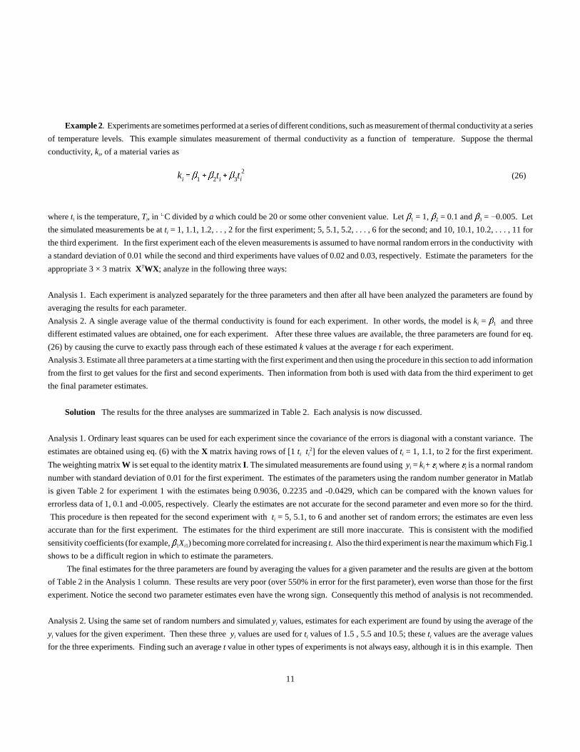
Example 2. Experiments are sometimes performed at a series of different conditions, such as measurement of thermal conductivity at a series
of temperature levels. This example simulates measurement of thermal conductivity as a function of temperature. Suppose the thermal
conductivity, ki, of a material varies as
where ti is the temperature, Ti, in (C divided by a which could be 20 or some other convenient value. Let �1 = 1, �2 = 0.1 and �3 = �0.005. Let
the simulated measurements be at ti = 1, 1.1, 1.2, . . , 2 for the first experiment; 5, 5.1, 5.2, . . . , 6 for the second; and 10, 10.1, 10.2, . . . , 11 for
the third experiment. In the first experiment each of the eleven measurements is assumed to have normal random errors in the conductivity with
a standard deviation of 0.01 while the second and third experiments have values of 0.02 and 0.03, respectively. Estimate the parameters for the
appropriate 3 × 3 matrix XTWX; analyze in the following three ways:
Analysis 1. Each experiment is analyzed separately for the three parameters and then after all have been analyzed the parameters are found by
averaging the results for each parameter.
Analysis 2. A single average value of the thermal conductivity is found for each experiment. In other words, the model is ki = �1 and three
different estimated values are obtained, one for each experiment. After these three values are available, the three parameters are found for eq.
(26) by causing the curve to exactly pass through each of these estimated k values at the average t for each experiment.
Analysis 3. Estimate all three parameters at a time starting with the first experiment and then using the procedure in this section to add information
from the first to get values for the first and second experiments. Then information from both is used with data from the third experiment to get
the final parameter estimates.
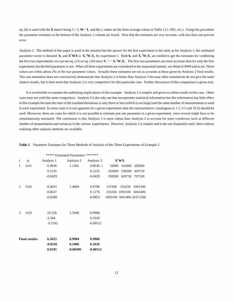
Solution The results for the three analyses are summarized in Table 2. Each analysis is now discussed.
Analysis 1. Ordinary least squares can be used for each experiment since the covariance of the errors is diagonal with a constant variance. The
estimates are obtained using eq. (6) with the X matrix having rows of [1 ti ti2] for the eleven values of ti = 1, 1.1, to 2 for the first experiment.
The weighting matrix W is set equal to the identity matrix I. The simulated measurements are found using yi = ki + Ji where Ji is a normal random
number with standard deviation of 0.01 for the first experiment. The estimates of the parameters using the random number generator in Matlab
is given Table 2 for experiment 1 with the estimates being 0.9036, 0.2235 and -0.0429, which can be compared with the known values for
errorless data of 1, 0.1 and -0.005, respectively. Clearly the estimates are not accurate for the second parameter and even more so for the third.
This procedure is then repeated for the second experiment with ti = 5, 5.1, to 6 and another set of random errors; the estimates are even less
accurate than for the first experiment. The estimates for the third experiment are still more inaccurate. This is consistent with the modified
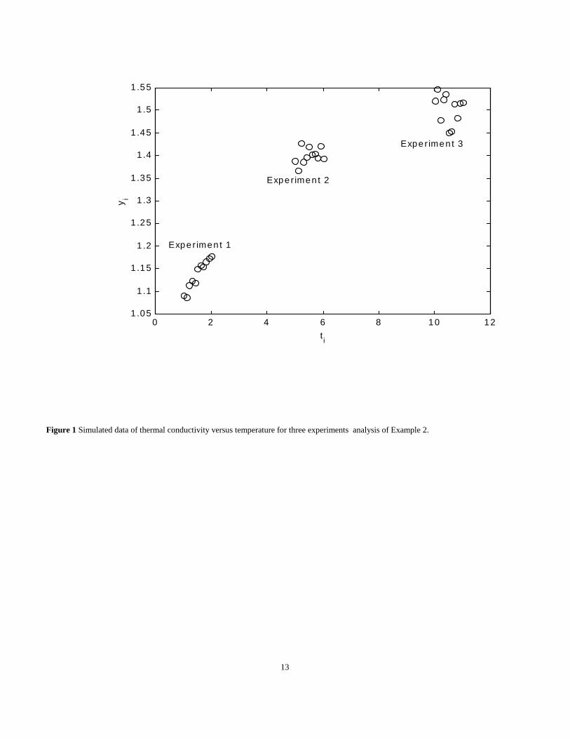
sensitivity coefficients (for example, �1Xi1) becoming more correlated for increasing t. Also the third experiment is near the maximum which Fig.1
shows to be a difficult region in which to estimate the parameters.
The final estimates for the three parameters are found by averaging the values for a given parameter and the results are given at the bottom
of Table 2 in the Analysis 1 column. These results are very poor (over 550% in error for the first parameter), even worse than those for the first
experiment. Notice the second two parameter estimates even have the wrong sign. Consequently this method of analysis is not recommended.
Analysis 2. Using the same set of random numbers and simulated yi values, estimates for each experiment are found by using the average of the
yi values for the given experiment. Then these three yi values are used for ti values of 1.5 , 5.5 and 10.5; these ti values are the average values
for the three experiments. Finding such an average t value in other types of experiments is not always easy, although it is in this example. Then
12
eq. (6) is used with the X matrix being 3 × 3, W = I, and the yi values are the three average values in Table 2 (1.1381, etc.). Using this procedure
the parameter estimates at the bottom of the Analysis 2 column are found. Note that the estimates are very accurate, with less than one percent
error.
Analysis 3. The method of this paper is used in the solution but the answer for the first experiment is the same as for Analysis 1; the estimated
parameter vector is denoted b1 and XTWX is X1TW1X1 for experiment 1. Both b1 and X1
TW1X1 are needed to get the estimates for combining
the first two experiments; we can use eq. (15) or eq. (16) since V1-1 = X1
TW1X1. The first two parameters are more accurate than for only the first
experiment, but the third parameter is not. When all three experiments are considered in the sequential manner, we obtain 0.9968 and so on. These
values are within about 2% of the true parameter values. Actually these estimates are not as accurate as those given by Analysis 2 final results.
This one simulation does not conclusively demonstrate that Analysis 2 is better than Analysis 3 because other simulations do not give the same
relative results, but it does seem that Analysis 2 is very competitive for this particular case. Further discussion of this comparison is given next.
It is worthwhile to examine the underlying implications of this example. Analysis 2 is simpler and gives excellent results in this case. Other
cases may not yield the same comparison. Analysis 3 is the only one that incorporates statistical information but this information has little effect
in this example because the ratio of the standard deviations is only three or less (which is not large) and the same number of measurements is used
in each experiment. In some cases it is not apparent for a given experiment what the representative t (analogous to 1.5, 5.5 and 10.5) should be
used. Moreover, there are cases for which it is not possible to estimate just one parameter in a given experiment, since several might have to be
simultaneously estimated The conclusion is that Analysis 3 is more robust than Analysis 2 to account for more conditions such as different
number of measurements and variances in the various experiments. However, Analysis 2 is simpler and is the one frequently used, often without
realizing other analysis methods are available.
Table 2 Parameter Estimates for Three Methods of Analysis of the Three Experiments of Example 2
***** Estimated Parameters *******
i )i Analysis 1 Analysis 2 Analysis 3 XTWX
1 0.01 0.9036 1.1381 0.9036 1 10000 165000 258500
0.2235 0.2235 165000 258500 420750
-0.0429 -0.0429 258500 420750 707330
2 0.02 -0.4631 1.4009 0.9706 137500 316250 1093100
0.6637 0.1176 316350 1093100 5041400
-0.0589 -0.0853 1093100 5041400 26371200
3 0.03 19.256 1.5048 0.9968
-3.364 0.1020
0.1592 -0.00512
Final results: 6.5655 0.9984 0.9968
-0.8256 0.1006 0.1020
0.0191 -0.00499 -0.00512
13
0 2 4 6 8 10 121 .05
1 .1
1 .15
1 .2
1 .25
1 .3
1 .35
1 .4
1 .45
1 .5
1 .55
ti
y i
Expe r imen t 1
Exper imen t 2
Exper imen t 3
Figure 1 Simulated data of thermal conductivity versus temperature for three experiments analysis of Example 2.
14
T(x,t)T0��qLk
1xL��
1Bi2M
�
j1exp(�2
j�t
L 2)(�2
j��Bi2)cos(� jx/L)
(�2j��Bi2
��Bi)�2j
(27)
T(x,t)T0��qLk
�t
L 2�
13
xL�
12
( xL
)2
2
%2M�
j1exp(%2j 2 �t
L 2) cos(%jx/L)
j 2 (28)
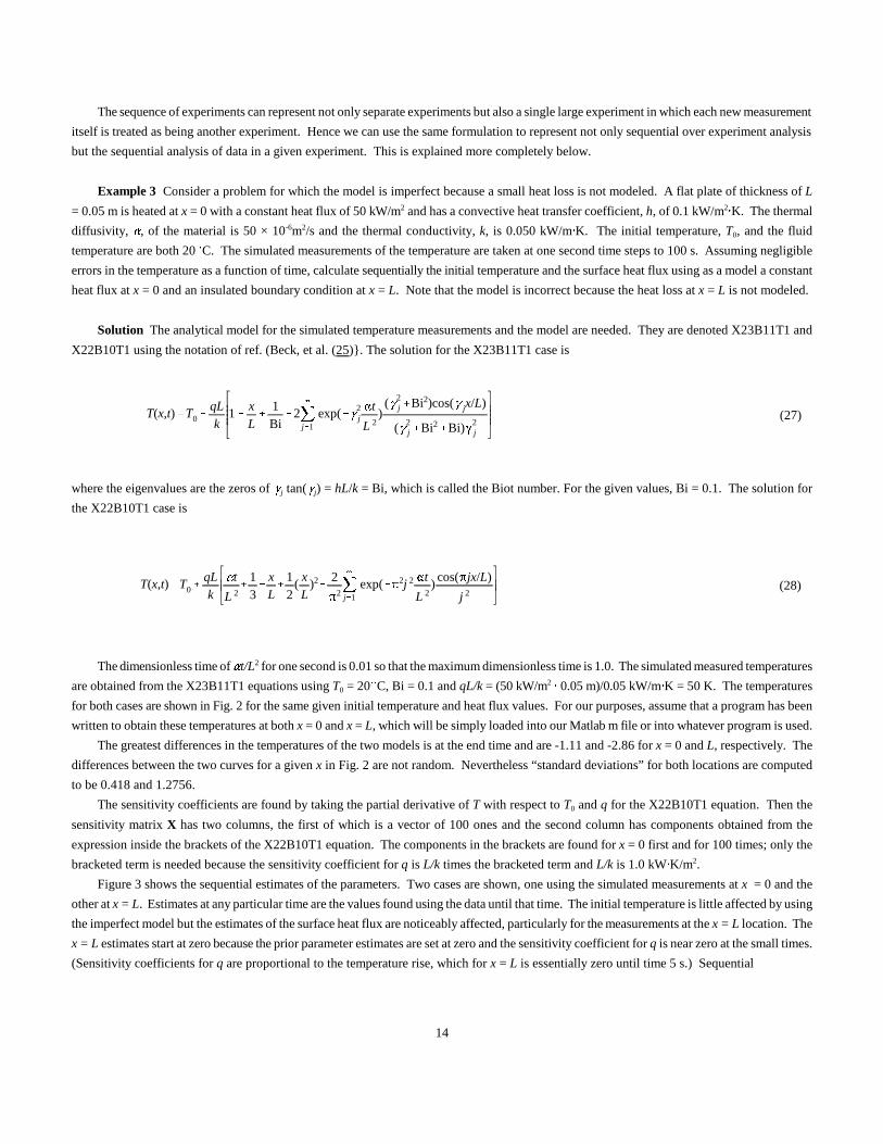
The sequence of experiments can represent not only separate experiments but also a single large experiment in which each new measurement
itself is treated as being another experiment. Hence we can use the same formulation to represent not only sequential over experiment analysis
but the sequential analysis of data in a given experiment. This is explained more completely below.
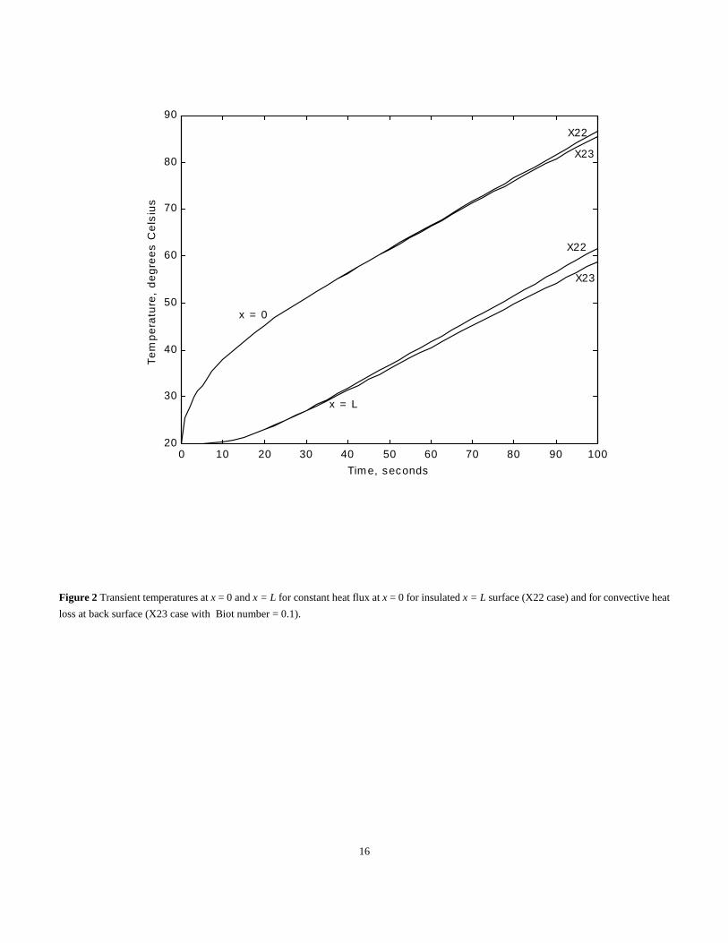
Example 3 Consider a problem for which the model is imperfect because a small heat loss is not modeled. A flat plate of thickness of L
= 0.05 m is heated at x = 0 with a constant heat flux of 50 kW/m2 and has a convective heat transfer coefficient, h, of 0.1 kW/m2#K. The thermal
diffusivity, �, of the material is 50 × 10-6m2/s and the thermal conductivity, k, is 0.050 kW/m#K. The initial temperature, T0, and the fluid
temperature are both 20(C. The simulated measurements of the temperature are taken at one second time steps to 100 s. Assuming negligible
errors in the temperature as a function of time, calculate sequentially the initial temperature and the surface heat flux using as a model a constant
heat flux at x = 0 and an insulated boundary condition at x = L. Note that the model is incorrect because the heat loss at x = L is not modeled.
Solution The analytical model for the simulated temperature measurements and the model are needed. They are denoted X23B11T1 and
X22B10T1 using the notation of ref. (Beck, et al. (25)}. The solution for the X23B11T1 case is
where the eigenvalues are the zeros of �j tan(�j) = hL/k = Bi, which is called the Biot number. For the given values, Bi = 0.1. The solution for
the X22B10T1 case is
The dimensionless time of �t/L2 for one second is 0.01 so that the maximum dimensionless time is 1.0. The simulated measured temperatures
are obtained from the X23B11T1 equations using T0 = 20(C, Bi = 0.1 and qL/k = (50 kW/m2 # 0.05 m)/0.05 kW/m#K = 50 K. The temperatures
for both cases are shown in Fig. 2 for the same given initial temperature and heat flux values. For our purposes, assume that a program has been
written to obtain these temperatures at both x = 0 and x = L, which will be simply loaded into our Matlab m file or into whatever program is used.
The greatest differences in the temperatures of the two models is at the end time and are -1.11 and -2.86 for x = 0 and L, respectively. The
differences between the two curves for a given x in Fig. 2 are not random. Nevertheless “standard deviations” for both locations are computed
to be 0.418 and 1.2756.
The sensitivity coefficients are found by taking the partial derivative of T with respect to T0 and q for the X22B10T1 equation. Then the
sensitivity matrix X has two columns, the first of which is a vector of 100 ones and the second column has components obtained from the
expression inside the brackets of the X22B10T1 equation. The components in the brackets are found for x = 0 first and for 100 times; only the
bracketed term is needed because the sensitivity coefficient for q is L/k times the bracketed term and L/k is 1.0 kW#K/m2.
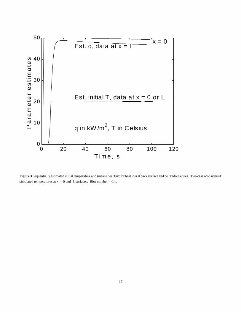
Figure 3 shows the sequential estimates of the parameters. Two cases are shown, one using the simulated measurements at x = 0 and the
other at x = L. Estimates at any particular time are the values found using the data until that time. The initial temperature is little affected by using
the imperfect model but the estimates of the surface heat flux are noticeably affected, particularly for the measurements at the x = L location. The
x = L estimates start at zero because the prior parameter estimates are set at zero and the sensitivity coefficient for q is near zero at the small times.
(Sensitivity coefficients for q are proportional to the temperature rise, which for x = L is essentially zero until time 5 s.) Sequential

15
estimates at x = L for larger times decrease with time. The largest error in the estimated q (neglecting the initial times) is at the end time when
the error is about -6.6% for the x = L case. The important point is that the q sequential estimates do not come to a constant in time but instead
continually change. Provided a sufficient number of measurements have been taken, a drifting downward or upward of parameter estimates after
the last half of the experimental time indicates an imperfect model. If caused by an imperfect model, this drifting behavior is frequently confirmed
by characteristic signatures in the residuals. Characteristic signatures are repeated in successive experiments and are apparent with different sets
of random errors.
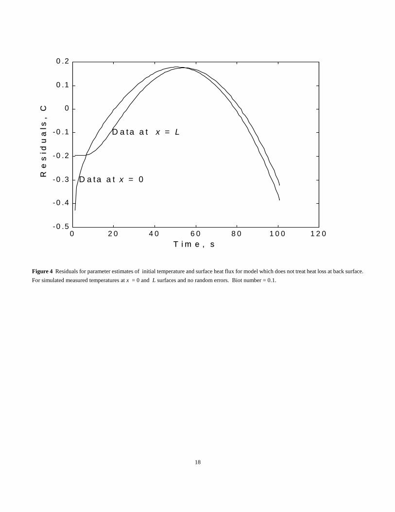
Figure 4 shows the residuals for both the x = 0 and x = L cases. The residuals happen to be nearly the same shape and magnitude. If small
random errors are present, the same characteristic shape of the residuals is observed. However, if the standard deviation of the simulated errors
is 0.3(C (about the maximum residual in Fig. 4 ) or larger, the characteristic signature may be difficult to discern.
The variation of the heat flux in Fig. 3 suggests that the true heat flux is not a constant but is time variable. Although it is actually constant,
investigate a possible time variation. For simplicity, consider the case of four constant segments. For zero random error measurements at x =
L, the estimated heat fluxes for the intervals of 0 to 25, 25 to 50, 50 to 75 and 75 to 100 s are 48.398, 46.502, 45.596 and 44.4, respectively. The
values for the correct model (X23) are all 50 kW/m2 so that the error becomes as large as -11%, which magnitude is almost twice as large as for
the constant q analysis. An important observation is that the use of an imperfect model can lead to the estimation of time-variable functions that
are less accurate than if the function is treated as a constant. It is possible that "more is not better than less". In parameter estimation,
parsimonious models are sought, that is, ones with the minimum number of parameters.
The presence of drifting parameters estimates near the end of the estimation time interval coupled with residual signatures indicates an
imperfect model. This imperfection can be in the physics of the model, such as not modeling heat loss. It could be that the process needs more
or different parameters, including treatment of a time-variable process. Engineering judgement is clearly needed in making these distinctions.
16
0 10 20 30 40 50 60 70 80 90 10020
30
40
50
60
70
80
90
Tim e, seconds
Te
mp
era
ture
, d
eg
ree
s C
els
ius
X22
X23
X22
X23
x = 0
x = L
Figure 2 Transient temperatures at x = 0 and x = L for constant heat flux at x = 0 for insulated x = L surface (X22 case) and for convective heat
loss at back surface (X23 case with Biot number = 0.1).
17
0 20 40 60 80 100 1200
10
20
30
40
50
T im e , s
Pa
ram
ete
r e
sti
ma
tes
x = 0Est. q, data at x = L
Est. initial T, data at x = 0 or L
q in kW /m2, T in Celsius
Figure 3 Sequentially estimated initial temperature and surface heat flux for heat loss at back surface and no random errors. Two cases considered:
simulated temperatures at x = 0 and L surfaces. Biot number = 0.1.
18
0 2 0 4 0 6 0 8 0 1 0 0 1 2 0-0 .5
-0 .4
-0 .3
-0 .2
-0 .1
0
0 .1
0 .2
T i m e , s
Re
sid
ua
ls,
C
D a ta a t x = L
D a ta a t x = 0
Figure 4 Residuals for parameter estimates of initial temperature and surface heat flux for model which does not treat heat loss at back surface.
For simulated measured temperatures at x = 0 and L surfaces and no random errors. Biot number = 0.1.
19
STik��(y��)TW(y��)�����THTH�� (29)
(y��)T(y��) (30)
H
1 1 0 á 0 0
0 1 1 á 0 0
� �
0 0 0 á 1 1
0 0 0 á 0 0
(31)
5. ILL-POSED PROBLEMS: TIKHONOV REGULARIZATION
Some physically important problems are ill-posed. Such problems are extremely sensitive to measurement errors. The use of prior
information, as in sequential over experiments, can stabilize these problems. In 1943 A.N. Tikhonov wrote a paper in Russian about the stability
of inverse problems (26) and in 1963 he published a paper on the regularization of ill-posed problems (27). His methods are related to using prior
information. However, his methods were not implemented in a sequential manner, which is possible and has important implications. The
Tikhonov approach is emphasized below but it is related to the methods described above.
The sum of squares function that is minimized in the Tikhonov method is
where �� is the model vector, � is the Tikhonov regularization parameter, and H depends upon the order of regularization (which is discussed more
below) . Notice that eq. (29) is the same as eq. (12) if b1 is 0 and V-1 is set equal to �HTH. In general, if little prior information is available, V
is chosen to be diagonal with large diagonal components and then the inverse would have small components on the diagonal. In Tikhonov
regularization, � is chosen to be small. More specifically, it is chosen such that the sum of squares given by
is reduced to the anticipated level, which is called in the Russian literature the discrepancy principle (8, 9). See also Osizik, (12), p. 607 and (22),
page 140. For the case of constant variance, uncorrelated errors, the expected the sum of squares is n)2. The Tikhonov parameter � is then chosen
to be about equal to this value.
One function estimation problem is the inverse heat conduction problem, which is the estimation of surface heat flux from interior
temperatures. This problem can be ill-posed when the time steps are small and there are about as many unknowns as measurements, or n is about
equal to p. In these cases the sum of squares function can be reduced to almost zero. As that condition is approached, however, the solution
becomes extremely sensitive to measurement errors, even becoming unstable. By not forcing the sum of squares to a minimum it is possible to
reduce oscillations and even stabilize the solution. In effect, one is introducing some bias to reduce the variance of the solution.
The matrix H can be different expressions corresponding to what is called zeroth order, first order and higher order regularization. Each of
these corresponds to difference approximations of derivatives of various orders. The zeroth order regularization is the most common and its H
is simply the identity matrix I; the effect of zeroth regularization is to bias the parameter estimates toward zero. The first order regularization
corresponds to the first derivative with time, if the desired function is a function of time. For first order regularization, H can be given by
This H biases the estimates toward a constant. For further discussion of H, see Beck, Blackwell and St. Clair, (22).
Minimizing eq. (29) gives in matrix notation,
20
bTik (XTWX��HTH)1XTWy (32)
As mentioned above, the matrix inverse in eq. (32) is shown for our understanding and not for computational purposes. This equation can also
be implemented in a sequential manner to yield important insights.
Example 4 A flat plate of thickness one unit thick is subjected at x = 0 to a constant heat flux of 0.2. The initial temperature is zero. The thermal
conductivity and thermal diffusivity are both unity. In each case the units are consistent. Except for the heat flux, the problem could be considered
in dimensionless terms. The surface at x = 1 is insulated. The temperature is measured at that surface at time steps of 0.06 and has uncorrelated
normal errors with a constant standard deviation of 0.0017. The standard statistical assumptions are valid. (The standard statistical assumptions
are listed in (1) and include additive, zero mean, constant variance, uncorrelated and normal errors.) The heat flux starts at time zero and continues
constant till the end of the period. Measurements are made at times -0.12, -0.06, 0.0, 0.06, . . ., 2.22 for a total of 40 measurements. From these
measurements the surface heat flux is to be estimated for each of the time steps using W = I with zeroth order regularization. The true heat flux
is zero until time zero and the constant value of 0.2 thereafter.
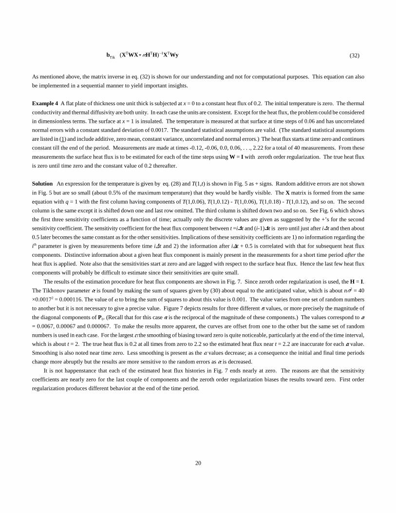
Solution An expression for the temperature is given by eq. (28) and T(1,t) is shown in Fig. 5 as + signs. Random additive errors are not shown
in Fig. 5 but are so small (about 0.5% of the maximum temperature) that they would be hardly visible. The X matrix is formed from the same
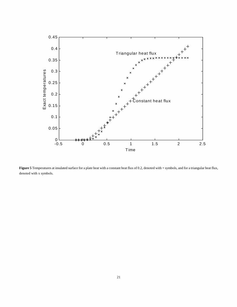
equation with q = 1 with the first column having components of T(1,0.06), T(1,0.12) - T(1,0.06), T(1,0.18) - T(1,0.12), and so on. The second
column is the same except it is shifted down one and last row omitted. The third column is shifted down two and so on. See Fig. 6 which shows
the first three sensitivity coefficients as a function of time; actually only the discrete values are given as suggested by the +’s for the second
sensitivity coefficient. The sensitivity coefficient for the heat flux component between t =i�t and (i-1)�t is zero until just after i�t and then about
0.5 later becomes the same constant as for the other sensitivities. Implications of these sensitivity coefficients are 1) no information regarding the
ith parameter is given by measurements before time i�t and 2) the information after i�t + 0.5 is correlated with that for subsequent heat flux
components. Distinctive information about a given heat flux component is mainly present in the measurements for a short time period after the
heat flux is applied. Note also that the sensitivities start at zero and are lagged with respect to the surface heat flux. Hence the last few heat flux
components will probably be difficult to estimate since their sensitivities are quite small.
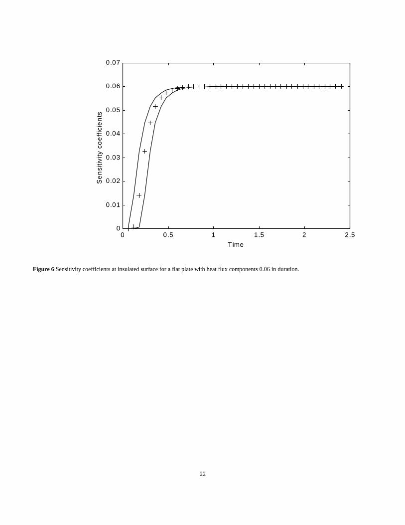
The results of the estimation procedure for heat flux components are shown in Fig. 7. Since zeroth order regularization is used, the H = I.
The Tikhonov parameter � is found by making the sum of squares given by (30) about equal to the anticipated value, which is about n)2 = 40
×0.00172 = 0.000116. The value of � to bring the sum of squares to about this value is 0.001. The value varies from one set of random numbers
to another but it is not necessary to give a precise value. Figure 7 depicts results for three different � values, or more precisely the magnitude of
the diagonal components of P0. (Recall that for this case � is the reciprocal of the magnitude of these components.) The values correspond to �
= 0.0067, 0.00067 and 0.000067. To make the results more apparent, the curves are offset from one to the other but the same set of random
numbers is used in each case. For the largest � the smoothing of biasing toward zero is quite noticeable, particularly at the end of the time interval,
which is about t = 2. The true heat flux is 0.2 at all times from zero to 2.2 so the estimated heat flux near t = 2.2 are inaccurate for each � value.
Smoothing is also noted near time zero. Less smoothing is present as the � values decrease; as a consequence the initial and final time periods
change more abruptly but the results are more sensitive to the random errors as � is decreased.
It is not happenstance that each of the estimated heat flux histories in Fig. 7 ends nearly at zero. The reasons are that the sensitivity
coefficients are nearly zero for the last couple of components and the zeroth order regularization biases the results toward zero. First order
regularization produces different behavior at the end of the time period.
21
-0.5 0 0.5 1 1.5 2 2.50
0.05
0.1
0.15
0.2
0.25
0.3
0.35
0.4
0.45
Time
Exa
ct t
em
pe
ratu
res
Constant heat flux
Triangular heat flux
Figure 5 Temperatures at insulated surface for a plate heat with a constant heat flux of 0.2, denoted with + symbols, and for a triangular heat flux,
denoted with x symbols.
22
0 0.5 1 1.5 2 2.50
0.01
0.02
0.03
0.04
0.05
0.06
0.07
Time
Se
nsi
tivity
co
eff
icie
nts
Figure 6 Sensitivity coefficients at insulated surface for a flat plate with heat flux components 0.06 in duration.
23
-0 .5 0 0.5 1 1.5 2 2.50
0.1
0.2
0.3
0.4
0.5
0.6
0.7
0.8
T ime, t
He
at
flu
x
P0 = 150I or α = 0 .0067, Est. q
P0 = 1500I or α = 0 .00067, Est. q + 0 .2
P0 = 15000I or α = 0 .000067, Est. q + 0 .4
Figure 7 Estimated heat flux as a function of time for the same set of random errors but three different values of P0 = 1/�I . The curves are offset
to enhance clarity.
24
�1(x�)�
13x �
�
(x �)2
2, �2(x
�)�1
45�
(x �)2
6
(x �)3
6�
(x �)4
24 (33b)
T(x �,t �)T0�qNL
k(t �)2
2��1(x
�)t ���2(x�)� 2
%4M�
j1
e j 2%
2t � cos(j%x �)
j 4 (33a)
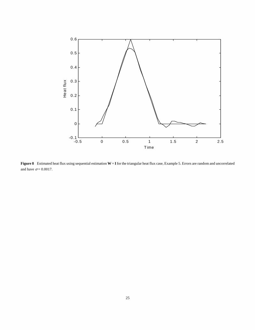
Example 5 Repeat Example 4 for the simulated temperatures at x = 1 resulting from a triangular heat flux which is zero before time zero when
it increases linearly to 0.6 at time 0.6. At time 0.6 it decreases linearly to 0 at time 1.2, after which it remains at zero. See the straight lines in
Fig. 8. As in the previous problem add random errors with a standard deviation of 0.0017 and estimate the heat flux components. Use sequential
estimation with W = I and display both the sequential results and final values.
Solution The simulated temperatures can be calculated using
where x+ � x/L and qN is the heat flux value at the Fourier number, �t/L2, of unity. In this problem, the initial temperature is equal to zero and t
has steps of 0.06 but x, L, �, qN and k are all unity. Superposition is used to obtain the triangular heat flux (22). The temperature history is shown
in Fig. 5.
Shown also in Fig. 8 is the estimated heat flux using the sequential method with W = I. The values shown are the final estimates for each
parameter when the data are all used. This curve is obtained using P0 = 765I, which corresponds to � equal to 1/765 = 0.00131. The triangular
heat flux is reproduced quite well in Fig. 8, with the most noticeable deviations from the true curve at the regions of abrupt change; namely, at
t = 0.0, 0.6 and 1.2. This example is an easier one than the previous example for zeroth order regularization because the estimated heat flux at
both the early and late times approaches zero. Incidentally the sequential method and the use of Matlab simultaneous solution for all the
parameters give final parameter estimates that agree within six or more significant figures, except possibly for the last few components.
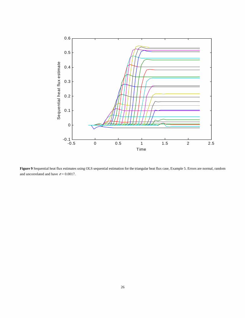
Figure 9 shows the sequential solutions of the heat flux components. The final values, that is, those at about t = 2.2, are the ones plotted in
Fig. 8. For each component in Fig. 9 the sequential estimates are zero until just after the time associated the component, then increase quite
rapidly, possibly overshoot slightly and finally remain constant until the final time. The time period over which each component changes seems
to be about 0.5, which is the same time period that the sensitivity coefficients are different as shown by Fig. 6. Insight into the solution can be
obtained from the sequential results shown in Fig. 9. For example, another sequential algorithm could be devised for this problem which would
not calculate any heat flux components until their time and then only calculate values for a time window of about 0.5 because the estimates are
constant thereafter. This insight cannot be obtained from an examination of Fig. 8 and gives a further advantage of the sequential method. For
further discussion of the inverse heat conduction problem, see (22).
Further Comments on Ill-posed Problems
Ill-posed problems may have very large numbers of parameters, 100's or even 10,000's. In such cases it may be appropriate to use some
iterative method of solution (such as given in (8)) and avoid the computation of individual sensitivity coefficients. However, the emphasis in this
paper is upon the estimation of parameters rather than estimation of functions, which often gives rise to ill-posed problems. In many of these
parameter estimation cases, ten or fewer parameters are simultaneous estimated, in which case the sensitivity coefficients are then needed and
efficiently used. The boundary between parameter and function estimation is not always clear, however.
25
-0.5 0 0.5 1 1.5 2 2.5-0.1
0
0.1
0.2
0.3
0.4
0.5
0.6
T ime
He
at
flu
x
Figure 8 Estimated heat flux using sequential estimation W = I for the triangular heat flux case, Example 5. Errors are random and uncorrelated
and have ) = 0.0017.
26
-0.5 0 0.5 1 1.5 2 2.5-0.1
0
0.1
0.2
0.3
0.4
0.5
0.6
Time
Se
qu
en
tial h
ea
t flu
x e
stim
ate
Figure 9 Sequential heat flux estimates using OLS sequential estimation for the triangular heat flux case, Example 5. Errors are normal, random
and uncorrelated and have ) = 0.0017.
27
��(��)��(b)� [//����
T (b)]T (��b)�à (34)
//���
0
0�1
�
0
0� p
(35)
S [y��(��)]T W[y��(��)]� (µ��)T V1(µ��) (36)
y
y(1)
y(2)
�
y(n)
where y(i)
y1(i)
y2(i)
�
ym(i)
(37)
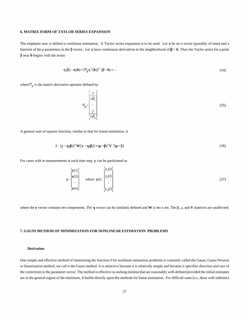
6. MATRIX FORM OF TAYLOR SERIES EXPANSION
The emphasis now is shifted to nonlinear estimation. A Taylor series expansion is to be used. Let �� be an n vector (possibly of time) and a
function of the p parameters in the �� vector. Let �� have continuous derivatives in the neighborhood of �� = b. Then the Taylor series for a point
�� near b begins with the terms
where is the matrix derivative operator defined by //��
A general sum of squares function, similar to that for linear estimation, is
For cases with m measurements at each time step, y can be partitioned as
where the y vector contains mn components. The �� vector can be similarly defined and W is mn x mn. The ��, )), and V matrices are unaffected.
7. GAUSS METHOD OF MINIMIZATION FOR NONLINEAR ESTIMATION PROBLEMS
Derivation
One simple and effective method of minimizing the function S for nonlinear estimation problems is variously called the Gauss, Gauss-Newton
or linearization method; we call it the Gauss method. It is attractive because it is relatively simple and because it specifies direction and size of
the corrections to the parameter vector. The method is effective in seeking minima that are reasonably well-defined provided the initial estimates
are in the general region of the minimum. It builds directly upon the methods for linear estimation. For difficult cases (i.e., those with indistinct
28
//��S2[//
���
T (��) ]W[y��(��) ]�2[I ]V1 (µ��) (38)
X(��)�[//���
T (��) ]T (39)
XT(�̂�)W[y��(�̂�) ]�V1 (µ �̂�)0 (40)
XT(b)W[y��(b)X(b) (�̂�b)]�V1 (µb)V1 (�̂�b)�0 (41)
b(k)b, b(k�1)
�̂�, ��(k)��(b), X(k)
X(b) (42)
b(k�1)b(k)
�P(k) [XT(k) W(y��(k))�V1 (µb(k))] (43a)
P1(k)�XT(k) WX(k)�V1 (43b)
minima) modifications to the Gauss method may be needed. Some of these modifications can be accommodated using eq. (36) which can include
prior information and Tikhonov regularization.
A necessary condition at the minimum of S is that the matrix derivative of S with respect to �� be equal to zero. For this reason operate
upon S to get
Let us use the notation X(��) for the sensitivity matrix,
so that eq. (38) set equal to zero at becomes�� �̂�
For nonlinear parameter estimation problems, we cannot directly solve for the estimator since appears implicitly in �� and X as well as�̂� �̂�
appearing explicitly. (An important observation is that if X is a function of the parameters, the problem is a nonlinear estimation problem.)
Suppose that we have an estimate of denoted b and that �� has continuous first derivatives in �� and bounded higher derivatives near b. Two�̂�
approximations are now used in eq. (40). First, replace X( ) by X(b) and second, use the first two terms of a Taylor series for about b.�̂ ��(�̂�)
Then eq. (40) becomes
Note that this equation is linear in . If a) �� is not too far from being linear in �� in a region about the solution to eq. (40) and if b) this region�̂�
includes b, the value of satisfying eq. (41) will be a better approximation to the solution eq. (40) than that provided by b. Assuming these two�̂�
conditions to be true, eq. (41) is set equal to the zero vector. Indicate an iterative procedure by
Using this notation in eq. (41) yields p equations in matrix form for b(k+1`) ,
w
29
b (k�1)i b (k)
i
b (k)i
< for i1,2,...,p (44)
X
X11 à X1p
� �
Xn1 à Xnp
0
0�1
�
0
0� p
�1 à � n
T
0�1
0�1
à0�1
0� p
� �
0� n
0�1
à0� n
0�P
(45)
�����X (k)
ij
0� i
0� j b(k)
(46)
� i�1 exp(�2ti)��3
hich is the Gauss linearization equation. Iteration on k is required for nonlinear models. For linear-in-the-parameters model no iterations are
required.
With this vector and can be calculated, which, in turn, are used in eq. (43a) to obtain the improved estimate vector This��(0) X(0) b(1).
completes the first iteration. Then and are evaluated so that can be found. The iterative procedure continues until there is negligible��(1) X(1) b(2)
change in any component of b; one criterion to indicate this is
where is a small number such as . When good initial estimates of the parameters are available and the experiment is well-designed, eq. (44)104
is frequently satisfied by the fifth iteration. (The fact that eq. (44) is satisfied does not guarantee that the last minimizes S, particularly whenb(k�1)
the minimum is ill-defined.)
As indicated above, the use of the matrix inverse is intended for our insight and not for computation. For well-designed experiments in
parameter estimation, the number of unknowns is not large and the solution at each step is not difficult. However, a sequential method of solution
is recommended in which the iterations are first performed until convergence. Then a final iteration is performed in the sequential manner
discussed above; it involves linearizing about the converged parameter values and shows parameter estimates as one measurement after another
is added. If desired, iterations before the final one can also be performed in a sequential manner but the detailed results are usually not displayed.
Sensitivity Matrix
Consider the sensitivity matrix as defined by eq. (39); without showing the dependence on b(k) , it can be written as
Hence the ij element of X(k) is
This definition of X is consistent with the linear model. A simple example is where has the same meaning as in eq. (5). A�i�1Xi1��2Xi2 Xij
model, nonlinear in its parameters, is
Its sensitivity coefficients are
30
Xi10� i
0�1
exp(�2ti), Xi20� i
0�2
�1 ti exp(�2ti), Xi3�1 (47)
kXi1k0Ti
0k, CXi1C
0Ti
0C,
(48)
k 0T0kT�Ts�
qLk�t
L 2, Ts�
qLk
2 �t
L 2M�
n1exp(n 2
%2�t/L 2)cos(n%x/L) (49)
C0T0C
TsqLL
�t
L 2 (50)
When one or more sensitivity coefficients are functions of the parameters, the estimation problem is nonlinear. This provides a powerful means
of determining if the problem is nonlinear. Note that only one sensitivity coefficient need be a function of the parameters to make the problem
nonlinear; even though Xi3 in the above example is not a function of any parameter (and hence the model is linear in terms of �3), the estimation
problem is still nonlinear.
Example 6 For a flat plate of thickness L = 1 and for a constant heat flux q of one at x = 0 and insulated at x = 1, the temperature is measured
at x = 1 with time steps of 0.05. (Consistent units or dimensionless quantities are used.) The thermal conductivity k and volumetric heat capacity
C are to be estimated using the simulated temperature measurements which are constructed for the exact temperatures for k = 1 and C = 1 with
additive errors with errors that have a standard deviation of ) = 0.0001. Another case is considered with ) = 0.01. First show the temperature
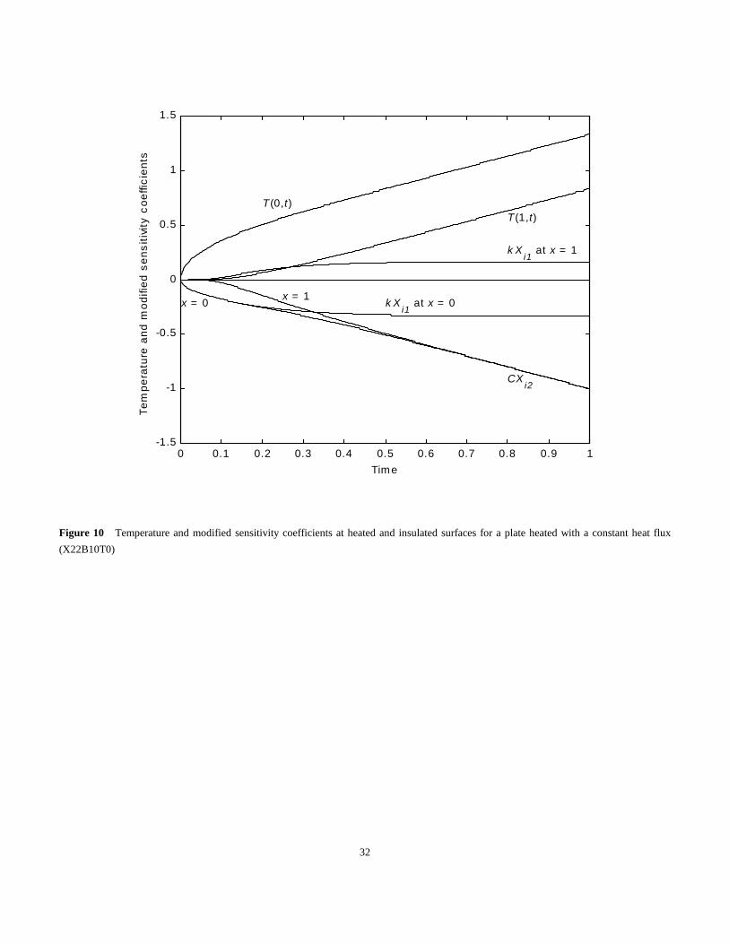
history and the modified sensitivity coefficients
which both have the units of temperature.
Solution The temperature solution is given by eq. (28) with the observation that � =k/C. Taking the derivative first with respect to k and then
with respect to C then give the modified sensitivity coefficients,
Notice that the sum of these two equations is the negative of the temperature rise. These modified sensitivity coefficients and the temperature
for both x = 0 and 1 (for an initial temperature of zero) are shown in Fig. 10.
The sensitivity coefficients for x = 0 are nearly equal for time t less than 0.25; this leads to the conclusion that it is impossible to estimate
simultaneously both k and C if only the surface temperature is measured until t = 0.25 or less. It is possible to estimate the product of k and C
for such measurements. Both modified sensitivity coefficients for x = 1 are negligible below the time of 0.1 and again the time must not be too
short to estimate both properties. For large times, the C sensitivities decrease linearly with time but those for k reach constant values. As a
consequence for very large times, the thermal conductivity will be inaccurately estimated compared to C. This suggests the need of optimal
experiments which would indicate an appropriate final time. See Beck and Arnold, (1), Chap. 8. From a comparison of the sensitivity coefficients
for x = 0 and 1, it is noted that the former would be a better experiment because the magnitude of the sensitivity coefficients are greater at x =0,
resulting in fewer iterations and smaller confidence regions on the average.

31
Using measurements at the insulated surface and with the standard deviations of 0.0001 and 0.01 (about 1% of the maximum temperature)
gives final conductivity and heat capacity estimates of 1.0003 and 1.0000 for ) = 0.0001 and for ) = 0.01 the estimates of 1.0323 and 1.0037.
For initial estimates for the iteration process, the wide range from one-half to double the true values is possible. For initial values of 2 for both
properties, nine iterations are needed.
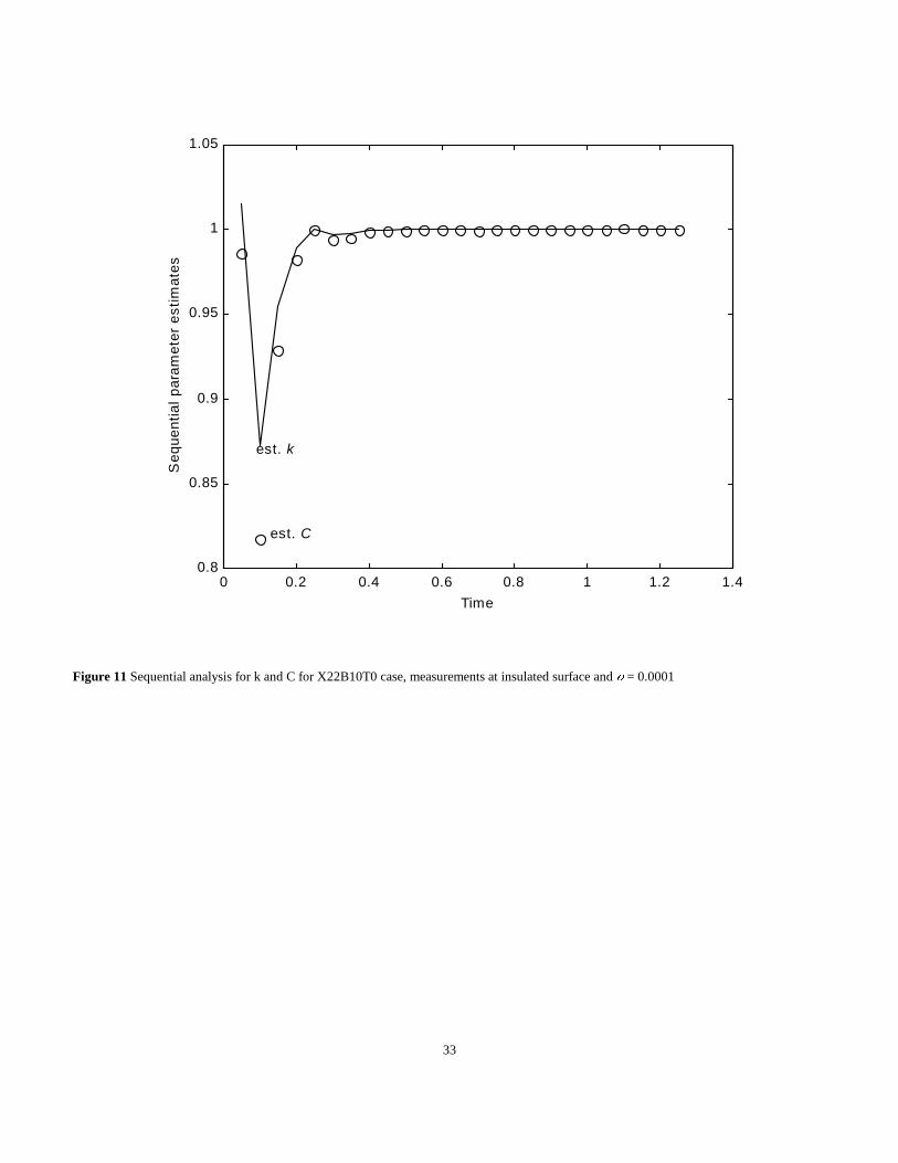
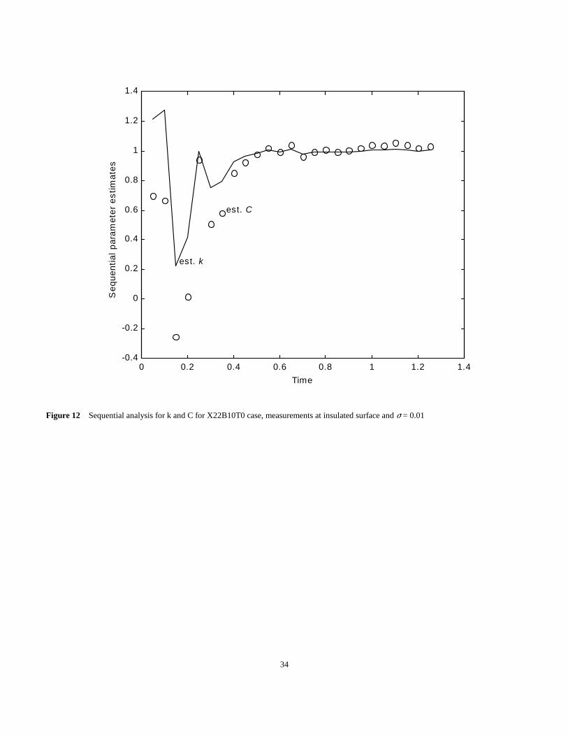
After the results are converged, a final iteration is performed to illustrate the effects of adding one measurement after another. See Figures
11 and 12. Some observations are now given.
1. Initial parameter estimates are needed and the path of the parameter values during the iterations depends upon the initial estimates.
2. This problem is not ill-posed.
3. The same final parameter estimates are found and are thus independent of the initial values in the range of at least .5 to 2.
4. The sequential estimates tend to constant values for the last half of the times shown. This is very important because it gives some
information about the adequacy of the model and an indication of the confidence region.
5. Considerable variations in the estimates are found at the earliest times, which is a result of the small sensitivity coefficients at those times.
6. As the standard deviations increase by a factor of 100, the error in the final estimates also increase by about the same factor.
32
0 0.1 0.2 0.3 0.4 0.5 0.6 0.7 0.8 0.9 1-1.5
-1
-0.5
0
0.5
1
1.5
T(0,t)
x = 1x = 0
k Xi1
at x = 1
k Xi1
at x = 0
CXi2
T(1,t)
Tim e
Te
mp
era
ture
an
d m
od
ifie
d s
en
sit
ivit
y c
oe
ffic
ien
ts
Figure 10 Temperature and modified sensitivity coefficients at heated and insulated surfaces for a plate heated with a constant heat flux
(X22B10T0)
33
0 0.2 0.4 0.6 0.8 1 1.2 1.40.8
0.85
0.9
0.95
1
1.05
Time
Se
que
ntia
l p
ara
me
ter
est
ima
tes
est. k
est. C
Figure 11 Sequential analysis for k and C for X22B10T0 case, measurements at insulated surface and ) = 0.0001
34
0 0.2 0.4 0.6 0.8 1 1.2 1.4-0.4
-0.2
0
0.2
0.4
0.6
0.8
1
1.2
1.4
Time
Se
qu
en
tia
l p
ara
me
ter
es
tim
ate
s
est. k
est. C
Figure 12 Sequential analysis for k and C for X22B10T0 case, measurements at insulated surface and ) = 0.01
35
cov(b)� (X TX)1s 2 (51)
bi bi <�i <bi� bi, bi t1�/2(np)(Cii)1/2s
bi bi <�i <bi� bi, bi t1�/2p(np)(Cii)1/2s
8. CONFIDENCE REGIONS
Confidence regions can be found using the sensitivity coefficients. The expression depends upon the statistical assumptions that are
applicable. One set of assumptions is that the measurement errors in temperature, for example, are additive, zero mean, constant variance,
uncorrelated and normal. For these assumptions, confidence regions can be given using the diagonals on the main diagonal of covariance matrix
of the measurement errors,
where s is the estimated standard deviation of the errors. For the ith parameter its confidence region can be given by
where the group Ciis2 is the estimated ith diagonal component of eq. (51) and t1-�/2(n-p) is the student’s t distribution for probability of 1-� and
n-p degrees of freedom. A common value of � is 0.05 which is for a 95% probability. If the joint probability confidence region is found, an
ellipse for two parameters is obtained and an ellipsoid for more parameters. However, ellipses or ellipsoids are difficult to use even though they
are more accurate than rectangular regions. Conservative joint confidence regions for rectangular regions given by the Bonferroni approximation
(3). The Bonferroni joint confidence regions are calculated using
with � = 0.05 for 95% probability and p is the number of parameters and n is the number of measurements (25 in the example). Notice the p in
the denominator of �/2p. For n-p and for 95% probability, t1-0.05/2p(�) is 2.0687 and 2.3979, for p = 1 and 2, respectively.
Example 7 For the same heat conduction example as in Example 6, investigate the confidence regions for additive, zero mean, uncorrelated,
normal errors with a standard deviation of ) = 0.01, which happens to be about 1% of the maximum temperature rise. Plot the estimates for a
Monte Carlo study for 1000 trials, that is, analyze for 1000 different sets of random errors. Also compare results for different numbers of trials
from 100 to 50,000, showing a comparison of the confidence intervals and regions for k and C with both the student’s t distribution and the
Bonferroni method.
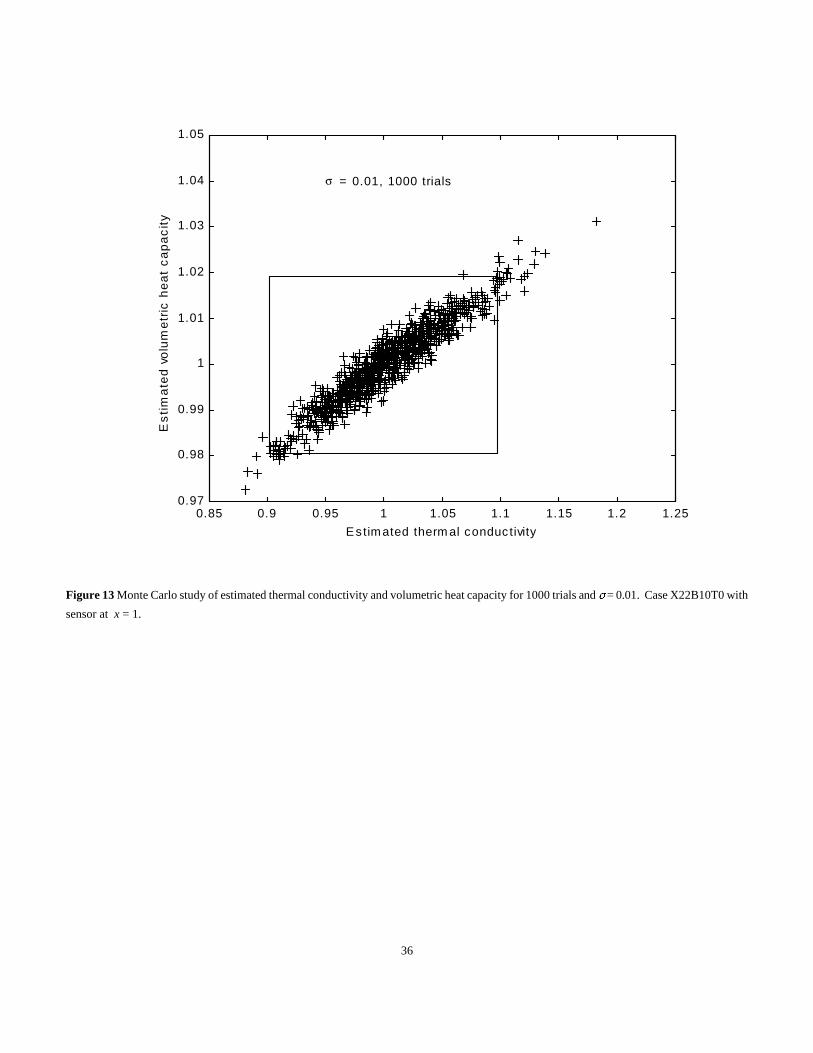
Solution Results of the estimates of 1000 simulations are shown in Fig. 13. Some observations are given next. The confidence region appears
to be elliptical in shape. It is not aligned along the major axes of k and C; consequently, when the estimated k or C is high or low, the other
parameter tends to be high or low. Also note that the plot does not have the same increments on both axes, so that the ellipse is distorted. The
average Bonferroni confidence region is also plotted; it looks square but to scale it would be more elongated in the horizontal axis. This region
indicates the region that should contain the true parameter estimates, (k = 1 and C = 1 in this example), for at least 95% of similar cases.
A summary of results of the Monte Carlo study is given in Table 3. Note that the student’s t distribution results for the confidence intervals
(for a single parameter) tend to be more accurate, but less conservative, than the Bonferroni results. However, the confidence region predicted
by the Bonferroni method is definitely more accurate than using the student’s t distribution. The Bonferroni confidence region is also conservative
since it is always less in Table 3 than the ideal values. The Bonferroni confidence region is rectangular in shape, not elliptical, so it is easier to
use but it includes large regions which are not very probable. See the northwest and southeast regions inside the rectangle of Fig. 13. Based on
this study, the Bonferroni confidence region is conservative and is easier to apply than the more rigorous elliptical confidence region implied by
Fig. 13. See (1) for a treatment of the ellipsoidal confidence region.
36
0.85 0.9 0.95 1 1.05 1.1 1.15 1.2 1.250.97
0.98
0.99
1
1.01
1.02
1.03
1.04
1.05
Estim ated therm al conductivity
Es
tim
ate
d v
olu
me
tric
he
at
ca
pa
cit
y
σ = 0.01, 1000 trials
Figure 13 Monte Carlo study of estimated thermal conductivity and volumetric heat capacity for 1000 trials and ) = 0.01. Case X22B10T0 with
sensor at x = 1.

37
Table 3 Results of Monte Carlo study for the student’s t and Bonferroni confidence intervals and regions for Example 7.
Values given are the number outside the estimated confidence intervals/regions. The left column is the number of trials and the next column
contains ideal number for an infinite number of trials.
No. Ideal k stud. C stud. Tot. Stud. k Bonf. C Bonf. Tot. Bonf.
100 5 6 5 7 3 2 3
500 25 36 37 44 18 18 23
1000 50 60 60 73 31 35 43
5000 250 287 299 379 150 157 209
50000 2500 3145 3062 3993 1659 1617 2165
Example 8 Investigate the parameter estimates of k and C for the above examples assuming heat losses are actually present (heat loss from x =
1 surface with Bi = 0.1) but are not modeled. (Using the conduction notation , the true model is X23B10T0 while it is modeled as X22B10T0.)
Solution The sequential estimated parameter estimates are shown by Fig. 14, where the final estimates are noted to be quite inaccurate. An
indication that the model is imperfect is that the sequential estimates tend to increase after the time of 0.5. The random errors for ) = 0.01 are
used but the final estimates are mainly affected by the imperfect model in this case. It is important to note the sequential results in Fig. 14 indicate
that the model is imperfect while, we shall see, the residuals may not reveal a modeling error unless the ) is made much smaller.
To examine the effects of the modeling error, see Table 4, third row. Notice that the parameter estimates for the Bonferroni confidence
region,
1.2371 < k < 1.3093 and 1.0947 < C < 1.1063
are well away from the true values of 1.0 and 1.0. This inaccurate confidence region is caused by the unmodeled heat losses. In this particular
example the parameter estimates are greatly affected by the modeling error but little affected by the simulated measurements errors, since ) =
0.01 and 0.0001 gave nearly the same parameter estimates. Table 4 also shows that the number of iterations is about 7 while it is 9 for no
modeling errors, for the initial estimates having the large values of 2 for all these calculations. It is also noteworthy that the estimated standard
deviation, s, for the ) = 0.0001, Bi = 0.1 case in Table 4 is much larger (by a factor of 27) than the true value of 0.0001. Hence, for this case the
use of the discrepancy principle to improve the parameter estimates would not be appropriate since it would suggest that the properties would
be a function of time or temperature, neither of which is actually true in this example.
Consider now the residuals for these two ) values. See Fig. 15. For ) = 0.0001, the residuals (indicated by the circles) are mainly affected
by the modeling error. We have a characteristic signature that would be repeated again and again for other sets of random errors with the same
). Note that the maximum amplitude occurs at the final time and is negative. That would be expected from the heat loss. See Fig. 4 which is
for a related case and has the same characteristic. Examining Fig. 15 reveals that the simulated errors for ) = 0.01 are so large that the underlying
characteristic signature is virtually invisible. However, it would become more apparent if many more cases (with ) =0.01) were run and the
residuals averaged. Careful examination of the residuals is a very powerful tool to investigate the model and character of the measurement errors.
It is highly recommended.
It should be noted that in addition to heat loss modeling errors, it is probable that inaccuracies will be present in the measurement of the
initial temperature distribution, surface heat flux, plate thickness and location of the temperature sensor. These will also make the correct
confidence region larger than given above.

38
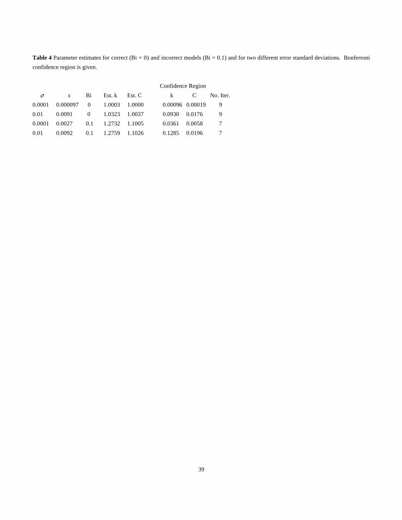
39
Table 4 Parameter estimates for correct (Bi = 0) and incorrect models (Bi = 0.1) and for two different error standard deviations. Bonferroni
confidence region is given.
Confidence Region
) s Bi Est. k Est. C k C No. Iter.
0.0001 0.000097 0 1.0003 1.0000 0.00096 0.00019 9
0.01 0.0091 0 1.0323 1.0037 0.0930 0.0176 9
0.0001 0.0027 0.1 1.2732 1.1005 0.0361 0.0058 7
0.01 0.0092 0.1 1.2759 1.1026 0.1285 0.0196 7
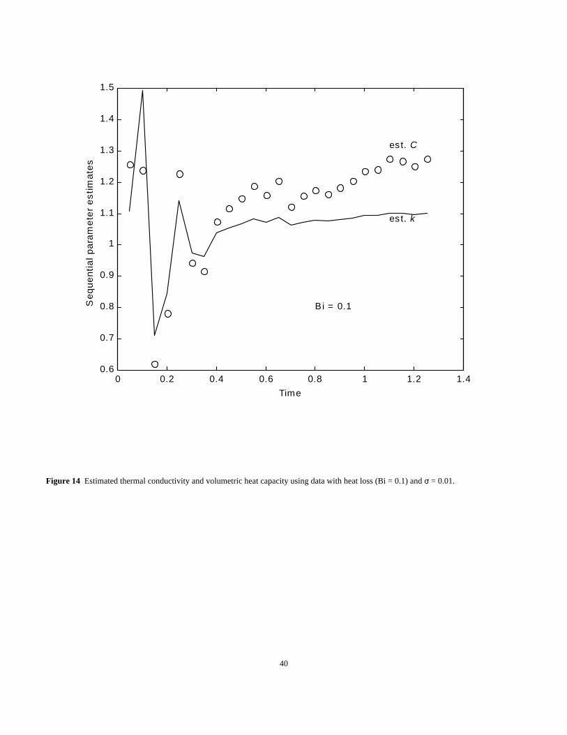
40
0 0.2 0.4 0.6 0.8 1 1.2 1.40.6
0.7
0.8
0.9
1
1.1
1.2
1.3
1.4
1.5
Time
Se
qu
en
tia
l p
ara
me
ter
es
tim
ate
s
es t. k
est. C
Bi = 0.1
Figure 14 Estimated thermal conductivity and volumetric heat capacity using data with heat loss (Bi = 0.1) and ) = 0.01.
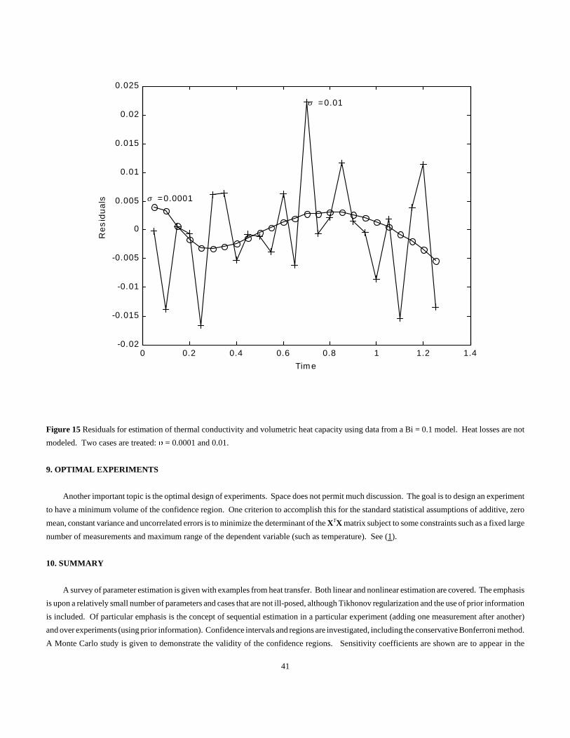
41
0 0.2 0.4 0.6 0.8 1 1.2 1.4-0.02
-0.015
-0.01
-0.005
0
0.005
0.01
0.015
0.02
0.025
Tim e
Re
sid
ua
ls σ =0.0001
σ =0.01
Figure 15 Residuals for estimation of thermal conductivity and volumetric heat capacity using data from a Bi = 0.1 model. Heat losses are not
modeled. Two cases are treated: ) = 0.0001 and 0.01.
9. OPTIMAL EXPERIMENTS
Another important topic is the optimal design of experiments. Space does not permit much discussion. The goal is to design an experiment
to have a minimum volume of the confidence region. One criterion to accomplish this for the standard statistical assumptions of additive, zero
mean, constant variance and uncorrelated errors is to minimize the determinant of the XTX matrix subject to some constraints such as a fixed large
number of measurements and maximum range of the dependent variable (such as temperature). See (1).
10. SUMMARY
A survey of parameter estimation is given with examples from heat transfer. Both linear and nonlinear estimation are covered. The emphasis
is upon a relatively small number of parameters and cases that are not ill-posed, although Tikhonov regularization and the use of prior information
is included. Of particular emphasis is the concept of sequential estimation in a particular experiment (adding one measurement after another)
and over experiments (using prior information). Confidence intervals and regions are investigated, including the conservative Bonferroni method.
A Monte Carlo study is given to demonstrate the validity of the confidence regions. Sensitivity coefficients are shown are to appear in the

42
estimation of parameters, determination of confidence regions and design of optimal experiments.
43
REFERENCES
1. Beck, J. V. and K. J. Arnold, Parameter Estimation in Engineering and Science, Wiley, New York, NY, 1977. (This book is out of print but
a paperback copy can be purchased from the first author.)
2. Bard, Y., Nonlinear Parameter Estimation, Academic Press, New York, NY, 1974.
3. Seber, G.A.F. and C.J. Wild, Nonlinear Regression, Wiley-lnterscience, 1989
4. Ross, G.J.S., Nonlinear Estimation, Springer-Verlag, NY, NY, 1990.
5. Goodwin, G.C. and R.L. Payne, Dynamic System Identification: Experiment Design and Data Analysis, Academic Press, NY, NY 1977.
6. Eykhoff, System Identification: Parameter and State Estimation, Wiley, NY, NY, 1974.
7. Ljung, L., System Identification, PrenticeHall PTR, Upper Saddle River, NJ, 1999.
8. Alifanov, O.M., Inverse Heat Transfer Problems, Springer-Verlag, New York, 1994.
9. Alifanov, O.M., E.A. Artyukhin and S.V. Rumyantsev, Extreme Methods for Solving III-Posed Problems with Application of Heat Transfer
Problems, Begell House, Inc., NY, 1 995.
10. Trujillo, D.M. and H.R. Busby, Practical Inverse Analysis in Engineering, CRC Press, NY, 1997 .
11. Hensel, E., Inverse Theory and Applications for Engineers, Prentice Hall, Englewood Cliffs, NJ, 1991.
12. Ozisik, M.N. Heat Conduction, Second Edition, Wiley-Interscience, NY, 1993.
13. Isakov, V., Inverse Problems for Partial Differential Equations, Springer-Verlag, New York, 1998.
14. Tarantola, A. Inverse Problem Theory: Methods for Data Fitting and Model Parameter Estimation, Elsevier NY, 1987.
15. Kurpisz, K. and A.J. Nowak, Inverse Thermal Problems, Computational Mechanics Publications, Boston, MA, 1995.
16. Bevington, P.R., Data Reduction and Error Analysis for the Physical Sciences, McGraw-Hill, NY, 1969.
17. Menke, W., Geophysical Data Analysis: Discrete Inverse Theory, Academic Press, NY, 1984.
18. Bjorck, A., Numerical Methods for Least Squares Problems, SIAM, Philadelphia, 1996.
19. Lawson, C.L. and R.J. Hanson, Solving Least Squares Problems, Prentice-Hall, Englewood Cliffs, NJ, 1974.
20. Box, G.E.P. and N.R. Draper, Empirical Model-Building and Response Surfaces, Wiley, NY, 1987.
21. Murio, D.A., The Mollification Method and the Numerical Solution of III-Posed Problems, Wiley-lnterscience, NY, 1993.
22. Beck, J. V., B. Blackwell, and C. R. St. Clair, Jr., Inverse Heat Conduction: III-Posed Problems, Wiley-lnterscience, NY, 1985. (This book
is out of print but a corrected paperback copy can be purchased from the first author.)
23. Tikhonov, A.N. and V.Y. Arsenin, Solutions of Ill-Posed Problems, V.H. Winston & Sons, NY, 1977.
24. Lamm, P.K., Personal communication, March 1999.
25. Beck, J.V., K. Cole, A. Haji-Sheikh, and B. Litkouhi, Heat Conduction Using Green's Functions, Hemisphere, Washington, D.C., 1992.
26. Tikhonov, A.N., The Stability of Inverse Problems, Doklady Akad. Nauk SSSR, Vol. 39, 1943.
27. Tikhonov, A.N., Regularization of Ill-posed Problems, Doklady Akad. Nauk SSSR, Vol. 153, 1963.