Sequential and joint hydrogeophysical inversion using a ...orbit.dtu.dk/files/81283751/hess_17_4043_2013.pdf · Herckenrath, Daan; Fiandaca, G.; Auken, Esben; Bauer-Gottwein, Peter

General rights Copyright and moral rights for the publications made accessible in the public portal are retained by the authors and/or other copyright owners and it is a condition of accessing publications that users recognise and abide by the legal requirements associated with these rights.

Users may download and print one copy of any publication from the public portal for the purpose of private study or research.

You may not further distribute the material or use it for any profit-making activity or commercial gain

You may freely distribute the URL identifying the publication in the public portal If you believe that this document breaches copyright please contact us providing details, and we will remove access to the work immediately and investigate your claim.

Downloaded from orbit.dtu.dk on: Feb 18, 2019

Sequential and joint hydrogeophysical inversion using a field-scale groundwatermodel with ERT and TDEM data

Herckenrath, Daan; Fiandaca, G.; Auken, Esben; Bauer-Gottwein, Peter

Published in:Hydrology and Earth System Sciences

Link to article, DOI:10.5194/hess-17-4043-2013

Publication date:2013

Document VersionPublisher's PDF, also known as Version of record

Link back to DTU Orbit

Citation (APA):Herckenrath, D., Fiandaca, G., Auken, E., & Bauer-Gottwein, P. (2013). Sequential and joint hydrogeophysicalinversion using a field-scale groundwater model with ERT and TDEM data. Hydrology and Earth SystemSciences, 17(10), 4043-4060. DOI: 10.5194/hess-17-4043-2013

https://doi.org/10.5194/hess-17-4043-2013

http://orbit.dtu.dk/en/publications/sequential-and-joint-hydrogeophysical-inversion-using-a-fieldscale-groundwater-model-with-ert-and-tdem-data(a0930918-2063-4c2f-89c8-4c5fa24c3150).html

Hydrol. Earth Syst. Sci., 17, 4043–4060, 2013www.hydrol-earth-syst-sci.net/17/4043/2013/doi:10.5194/hess-17-4043-2013© Author(s) 2013. CC Attribution 3.0 License.

Hydrology and Earth System

SciencesO

pen Access

Sequential and joint hydrogeophysical inversion using a field-scalegroundwater model with ERT and TDEM data

D. Herckenrath1,2, G. Fiandaca3,4, E. Auken3, and P. Bauer-Gottwein1

1Technical University of Denmark, Dept. of Environmental Engineering, Miljøvej, Building 113, 2800,Kgs. Lyngby, Denmark2Flinders University, National Centre for Groundwater Research and Training, G.P.O. Box 2100, Adelaide,SA 5001, Australia3Aarhus University, Dept. of Earth Sciences, Høegh-Guldbergs Gade 2, 8000, Aarhus C, Denmark4University of Palermo, Dept. of Mathematics and Computer Science, Palermo, Italy

Correspondence to:D. Herckenrath ([email protected])

Received: 1 February 2013 – Published in Hydrol. Earth Syst. Sci. Discuss.: 11 April 2013Revised: 28 August 2013 – Accepted: 11 September 2013 – Published: 18 October 2013

Abstract. Increasingly, ground-based and airborne geophys-ical data sets are used to inform groundwater models. Re-cent research focuses on establishing coupling relationshipsbetween geophysical and groundwater parameters. To fullyexploit such information, this paper presents and comparesdifferent hydrogeophysical inversion approaches to inform afield-scale groundwater model with time domain electromag-netic (TDEM) and electrical resistivity tomography (ERT)data. In a sequential hydrogeophysical inversion (SHI) agroundwater model is calibrated with geophysical data bycoupling groundwater model parameters with the invertedgeophysical models. We subsequently compare the SHI witha joint hydrogeophysical inversion (JHI). In the JHI, a geo-physical model is simultaneously inverted with a groundwa-ter model by coupling the groundwater and geophysical pa-rameters to explicitly account for an established petrophysi-cal relationship and its accuracy. Simulations for a syntheticgroundwater model and TDEM data showed improved esti-mates for groundwater model parameters that were coupledto relatively well-resolved geophysical parameters when em-ploying a high-quality petrophysical relationship. Comparedto a SHI these improvements were insignificant and geophys-ical parameter estimates became slightly worse. When em-ploying a low-quality petrophysical relationship, groundwa-ter model parameters improved less for both the SHI and JHI,where the SHI performed relatively better. When comparinga SHI and JHI for a real-world groundwater model and ERTdata, differences in parameter estimates were small. For both

cases investigated in this paper, the SHI seems favorable, tak-ing into account parameter error, data fit and the complexityof implementing a JHI in combination with its larger compu-tational burden.

1 Introduction

Over the last decade, interest in geophysical methods forhydrogeological site characterization has been increasing(Vereecken et al., 2004; Hubbard and Rubin, 2000). This isdue to the ability of geophysical methods to provide mod-els of subsurface properties with a high spatial resolution,which are difficult to obtain from sparse borehole informa-tion. Worldwide, significant resources are spent on the col-lection of regional geophysical data sets. Examples includeairborne electromagnetic (AEM) surveys in Denmark, cov-ering nearly 60 % of the country for mapping the spatial ex-tent and assessing the vulnerability of aquifers (Thomsen etal., 2004), and AEM surveys to map saltwater intrusion inthe USA, Australia, Germany and the Netherlands (Langevinet al., 2003; Fitzpatrick et al., 2009; Faneca Sànchez et al.,2012; Burschil et al., 2012). In addition, smaller-scale sur-veys have been conducted using a variety of geophysicaltechniques such as ERT (electrical resistivity tomography,Kemna et al., 2002), induced polarization (Slater, 2007) andmagnetic resonance sounding (Legchenko and Valla, 2002).

Published by Copernicus Publications on behalf of the European Geosciences Union.

4044 D. Herckenrath et al.: Sequential and joint hydrogeophysical inversion

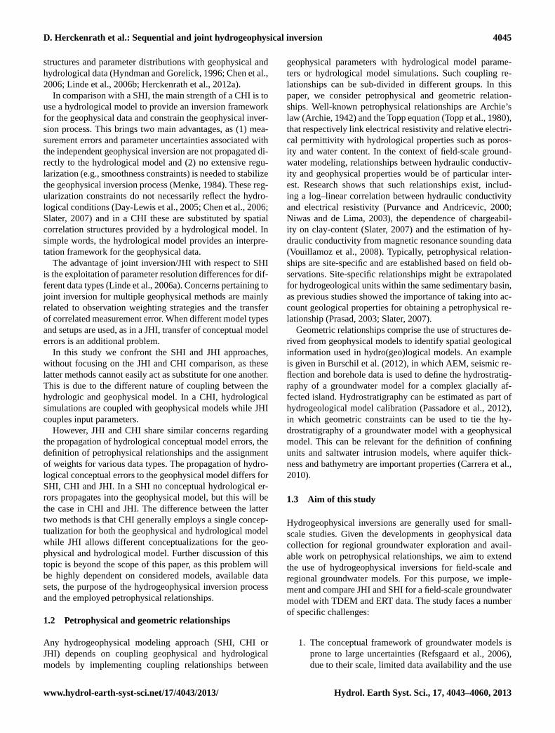
1 2 Fig. 1 SHI (left), CHI (middle) and JHI approach (right). π and γ respectively indicate the geophysical and groundwater model parameters, where the 3 arrows represent parameter updating until a minimum data and/or constraint misfit is achieved. π: geophysical model parameters; γ: groundwater model 4 parameters. 5

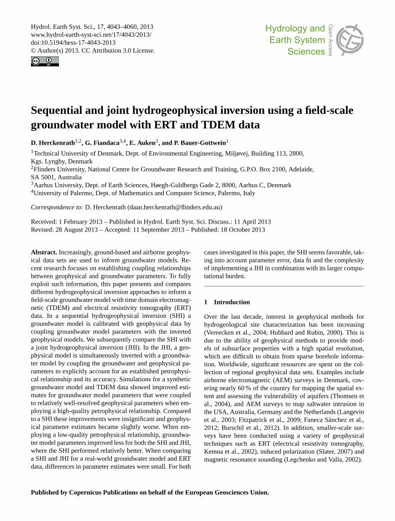
Fig. 1.SHI (left), CHI (middle) and JHI approach (right).π andγ respectively indicate the geophysical and groundwater model parameters,where the arrows represent parameter updating until a minimum data and/or constraint misfit is achieved.π : geophysical model parameters;γ : groundwater model parameters.

A major challenge is to fully exploit the information con-tent of geophysical data sets, as geophysical techniques donot measure hydrological subsurface properties directly. Ageophysical inversion and petrophysical relationships areneeded to estimate hydrogeological parameters and statevariables from the geophysical data sets. For this reason,the inclusion of geophysical data into a groundwater modelis not straightforward. Previous studies have used differentapproaches to inform groundwater models with geophysicaldata.

1.1 Hydrogeophysical inversion approaches

Hydrogeophysical inversion approaches can be subdividedinto sequential hydrogeophysical inversion (SHI), coupledhydrogeophysical inversion (CHI) and joint hydrogeophys-ical inversion (JHI) (Hinnell et al., 2010). The workflow as-sociated with these 3 methods is shown in Fig. 1.

1. In a SHI, geophysical data is separately inverted to es-timate the distribution of a geophysical property (e.g.,maps of electrical resistivity). Estimated geophysicalproperty maps are subsequently used to derive thestructure of the subsurface or to estimate dynamicstate variables such as solute concentrations and wa-ter content. For the latter, petrophysical relationships(Archie, 1942; Topp et al., 1980) are needed to converta geophysical property to a hydrological state variable.Note Fig. 1 only shows an SHI in which inverted geo-physical parameters are coupled with the static inputstructure of a hydrological model; SHI by couplingdynamic state variables would typically require cou-pling inverted geophysical parameters with hydrologicmodel output.

2. In a CHI, simulated state variables of a hydrologi-cal model are transformed to a geophysical parameterdistribution using a petrophysical relationship. Subse-quently, geophysical forward responses are simulatedthat can be compared with collected geophysical ob-servations. In this approach, the geophysical inversion

process is coupled with the hydrological model and asingle objective function is minimized that comprisesboth a geophysical and a hydrological component.

3. In a JHI, a simultaneous inversion for multiple geo-physical and/or hydrological models is undertaken toexploit differences in parameter resolution for differ-ent data sets. In the JHI discussed in this paper, inputparameters of a hydrological and geophysical modelare simultaneously estimated using parameter cou-pling constraints to account for observed correlationsbetween geophysical and groundwater model parame-ters (e.g., petrophysical relationships).

Examples of SHI applications include the use of geoelec-trical methods, electromagnetic methods and ground pene-trating radar (GPR) to monitor changes in soil water con-tent or solute concentrations with time (Binley et al., 2001;Cassiani et al., 2006; Day-Lewis et al., 2003; Huisman etal., 2003; Kemna et al., 2002; Knight, 2001; Looms et al.,2008). Of particular interest is the SHI framework presentedby Dam and Christensen (2003) in which inverted electri-cal resistivities are used to estimate hydraulic conductivityfields of a groundwater model. As will be explained later,our JHI approach shows many similarities with this frame-work. Examples of CHI applications include the estimationof vadose zone parameters with electrical resistivity and GPRmeasurements (Hinnell et al., 2010; Kowalsky et al., 2005;Lambot et al., 2006, 2009), the estimation of hydraulic con-ductivity fields with electrical resistivity data (Pollock andCirpka, 2012) and the estimation of soil properties withrelative gravimetry and magnetic resonance sounding data(Christiansen et al., 2011; Herckenrath et al., 2012a). Thesestudies cover a relatively small spatial scale compared tofield-scale groundwater models. Applications of a CHI on amore regional scale can be found in (Bauer-Gottwein et al.,2010; Herckenrath et al., 2012b). JHI methods have been de-veloped to use multiple geophysical methods for estimatingsoil properties (Vozoff and Jupp, 1975; Linde et al., 2006a;Behroozmand et al., 2012) or to jointly estimate hydrological

Hydrol. Earth Syst. Sci., 17, 4043–4060, 2013 www.hydrol-earth-syst-sci.net/17/4043/2013/

D. Herckenrath et al.: Sequential and joint hydrogeophysical inversion 4045

structures and parameter distributions with geophysical andhydrological data (Hyndman and Gorelick, 1996; Chen et al.,2006; Linde et al., 2006b; Herckenrath et al., 2012a).

In comparison with a SHI, the main strength of a CHI is touse a hydrological model to provide an inversion frameworkfor the geophysical data and constrain the geophysical inver-sion process. This brings two main advantages, as (1) mea-surement errors and parameter uncertainties associated withthe independent geophysical inversion are not propagated di-rectly to the hydrological model and (2) no extensive regu-larization (e.g., smoothness constraints) is needed to stabilizethe geophysical inversion process (Menke, 1984). These reg-ularization constraints do not necessarily reflect the hydro-logical conditions (Day-Lewis et al., 2005; Chen et al., 2006;Slater, 2007) and in a CHI these are substituted by spatialcorrelation structures provided by a hydrological model. Insimple words, the hydrological model provides an interpre-tation framework for the geophysical data.

The advantage of joint inversion/JHI with respect to SHIis the exploitation of parameter resolution differences for dif-ferent data types (Linde et al., 2006a). Concerns pertaining tojoint inversion for multiple geophysical methods are mainlyrelated to observation weighting strategies and the transferof correlated measurement error. When different model typesand setups are used, as in a JHI, transfer of conceptual modelerrors is an additional problem.

In this study we confront the SHI and JHI approaches,without focusing on the JHI and CHI comparison, as theselatter methods cannot easily act as substitute for one another.This is due to the different nature of coupling between thehydrologic and geophysical model. In a CHI, hydrologicalsimulations are coupled with geophysical models while JHIcouples input parameters.

However, JHI and CHI share similar concerns regardingthe propagation of hydrological conceptual model errors, thedefinition of petrophysical relationships and the assignmentof weights for various data types. The propagation of hydro-logical conceptual errors to the geophysical model differs forSHI, CHI and JHI. In a SHI no conceptual hydrological er-rors propagates into the geophysical model, but this will bethe case in CHI and JHI. The difference between the lattertwo methods is that CHI generally employs a single concep-tualization for both the geophysical and hydrological modelwhile JHI allows different conceptualizations for the geo-physical and hydrological model. Further discussion of thistopic is beyond the scope of this paper, as this problem willbe highly dependent on considered models, available datasets, the purpose of the hydrogeophysical inversion processand the employed petrophysical relationships.

1.2 Petrophysical and geometric relationships

Any hydrogeophysical modeling approach (SHI, CHI orJHI) depends on coupling geophysical and hydrologicalmodels by implementing coupling relationships between

geophysical parameters with hydrological model parame-ters or hydrological model simulations. Such coupling re-lationships can be sub-divided in different groups. In thispaper, we consider petrophysical and geometric relation-ships. Well-known petrophysical relationships are Archie’slaw (Archie, 1942) and the Topp equation (Topp et al., 1980),that respectively link electrical resistivity and relative electri-cal permittivity with hydrological properties such as poros-ity and water content. In the context of field-scale ground-water modeling, relationships between hydraulic conductiv-ity and geophysical properties would be of particular inter-est. Research shows that such relationships exist, includ-ing a log–linear correlation between hydraulic conductivityand electrical resistivity (Purvance and Andricevic, 2000;Niwas and de Lima, 2003), the dependence of chargeabil-ity on clay-content (Slater, 2007) and the estimation of hy-draulic conductivity from magnetic resonance sounding data(Vouillamoz et al., 2008). Typically, petrophysical relation-ships are site-specific and are established based on field ob-servations. Site-specific relationships might be extrapolatedfor hydrogeological units within the same sedimentary basin,as previous studies showed the importance of taking into ac-count geological properties for obtaining a petrophysical re-lationship (Prasad, 2003; Slater, 2007).

Geometric relationships comprise the use of structures de-rived from geophysical models to identify spatial geologicalinformation used in hydro(geo)logical models. An exampleis given in Burschil et al. (2012), in which AEM, seismic re-flection and borehole data is used to define the hydrostratig-raphy of a groundwater model for a complex glacially af-fected island. Hydrostratigraphy can be estimated as part ofhydrogeological model calibration (Passadore et al., 2012),in which geometric constraints can be used to tie the hy-drostratigraphy of a groundwater model with a geophysicalmodel. This can be relevant for the definition of confiningunits and saltwater intrusion models, where aquifer thick-ness and bathymetry are important properties (Carrera et al.,2010).

1.3 Aim of this study

Hydrogeophysical inversions are generally used for small-scale studies. Given the developments in geophysical datacollection for regional groundwater exploration and avail-able work on petrophysical relationships, we aim to extendthe use of hydrogeophysical inversions for field-scale andregional groundwater models. For this purpose, we imple-ment and compare JHI and SHI for a field-scale groundwatermodel with TDEM and ERT data. The study faces a numberof specific challenges:

1. The conceptual framework of groundwater models isprone to large uncertainties (Refsgaard et al., 2006),due to their scale, limited data availability and the use

www.hydrol-earth-syst-sci.net/17/4043/2013/ Hydrol. Earth Syst. Sci., 17, 4043–4060, 2013


of many simplifying assumptions associated with thegeological model and boundary conditions.

2. The sub-surface volumes represented by groundwaterand geophysical models can be very different, whichlimits using a single conceptualization for both mod-els.

3. Some subsurface processes and/or compartments areincluded in the geophysical or hydrogeological modelonly and are not represented in the other model.

4. The accuracy of the relationship between geophysicaland groundwater model parameters is difficult to de-termine.

5. Computational burden and large number of estimatedparameters.

6. Correlated geophysical measurement error.

Based on the first three issues, geophysical and hydrogeo-logical models usually require different conceptualizationsto achieve an acceptable data fit. This flexibility cannot beincorporated when the geophysical model is completely con-structed from hydrological model in- or output as in manyCHI studies.

The strength of coupling between the geophysical andgroundwater models is difficult to determine and can bebased on the assumed accuracy of the (petro)physical rela-tionships between geophysical and groundwater properties.This accuracy can be estimated from correlating geophysi-cal models with available groundwater data (e.g., pumpingtests, borehole data, and lab tests). In a SHI the strength ofcoupling constraints can be either based on geophysical pa-rameter resolution or the accuracy of the petrophysical rela-tionship.

The fifth challenge is related to the large computationalburden associated with groundwater models and inversionof geophysical models. Due to the computational burden,parameter estimation is typically performed using local,gradient-search algorithms (Doherty, 2010) instead of globalsearch algorithms like Markov–Chain Monte Carlo basedmethods (Vrugt et al., 2009). Gradient-search algorithms,such as the Levenberg–Marquardt method, do not alwaysfind the true global minimum of the objective function sur-face due to multiple local minima in parameter space, discon-tinuous first derivatives, curved multidimensional ridges andparameter surrogacy (Vrugt et al., 2008). Initial parametervalues are therefore extremely important when using local,gradient-search techniques.

The final challenge refers to correlated geophysical mea-surement errors that can be caused by existing infrastructure(e.g., power lines, buried pipes), neglecting 3-D effects in thegeophysical model (Bauer-Gottwein et al., 2010) and the ap-plication of inaccurate/limited instrument filters when pro-cessing geophysical data (Efferso et al., 1999). Character-istics of correlated noise are location-specific and different

for the various types of geophysical methods and thereforedifficult to quantify. We do not consider correlated measure-ment error in this paper. An example of how correlated mea-surement error propagates in a CHI is provided in Hinnell etal. (2010) and Herckenrath et al. (2012a).

To meet the previous mentioned challenges, we implementa SHI and JHI in which geophysical model parameters aretied to groundwater model parameters by adding parametercoupling constraints. These parameter coupling constraintscan be imposed to subsets of parameters to ensure enoughflexibility to fit the different types of observation data, whilethe imposed strength of the parameter coupling constraintsreflects the quality of the relationship between model pa-rameters that can be derived from field data or geophysi-cal parameter resolution. Finally, these parameter couplingconstraints are compatible with standard inversion methodsused for groundwater and geophysical models. The presentedSHI-approach is similar to Dam and Christensen (2003),whereas the JHI is similar to an inversion methodology usedby Doherty and Johnston (2003), which differs from standardjoint inversion approaches, as input parameters are not sharedby multiple models but coupled through additional regular-ization constraints.

Section 2 provides a theoretical background for the appliedSHI and JHI. Section 3 shows the application of both the SHIand JHI for a synthetic groundwater model with time domainelectromagnetic (TDEM) data. The implementation of a JHIand SHI for a real-world groundwater model and geoelec-tric data (ERT) is described in Sect. 4. Results are given interms of parameter estimates, parameter error, model misfitand computational burden. The paper concludes with a sum-mary of the benefits, disadvantages and limitations associ-ated with the presented coupling procedures.

2 Methodology

This section provides a mathematical summary of a SHI andJHI.

2.1 Sequential hydrogeophysical inversion (SHI)

The SHI starts with a geophysical inversion. Consider a dataset of geophysical observations assembled in vectordg:

dg =(ρ1,ρ2, .,ρNg

)T+ eg. (1)

The symbolρ denotes the geophysical observations, e.g.,apparent resistivities. SubscriptNg is the number of avail-able geophysical observations andeg denotes the geophys-ical measurement error. The geophysical model parametersthat are estimated are assembled in vectorπ :

π = (r1, ., rMr , t1., tMt)T . (2)

In this paperπ contains a number of layer thicknesses(t) and layer resistivities (r) for a 1-D electrical resistivity



model.Mr andMt represent the number of parameters foreach parameter type and their sum (Mr + Mt) is representedby Mg.

The SHI starts with a geophysical inversion in which geo-physical parameters inπ are estimated by fitting the geo-physical observations indg. For this purpose we follow awell-established iterative least-squares inversion approach(Tarantola and Valette, 1982; Menke, 1984).

According to Auken and Christiansen (2004), the inver-sion problem can be written as

GgIPhRpRh

· δπ =

δdgδπpriorδπh-priorδrpδrh

+

egeprioreh-priorepeh

. (3)

In the geophysical inversion, a geophysical forward modelis used to calculate apparent resistivities for the electricalresistivity model defined inπ . Gg is the Jacobian compris-ing the partial derivatives ofdg with respect to the geo-physical parameters inπ . Furthermore, four types of regu-larization constraints are used in the inversion: prior param-eter constraints, prior depth constraints, vertical constraintsand lateral constraints. These result in four additional oper-atorsI , Ph, Rp andRh and contribute to the total geophys-ical observation errore′

g. The implementation and deriva-tion of these constraints is explained in detail in Auken andChristiansen (2004).δπprior, δπh-prior, δrp and δrh expressthe deviation with respect to the expected value for the priorparameter constraints, prior depth constraints, vertical con-straints and lateral constraints.eprior, eh-prior, ep, andeh arethe errors associated with these constraints. More compactEq. (3) is

G′g · δπ = δd ′

g + e′g. (4)

In the geophysical inversion the following objective func-tion is minimized by updatingπ ,

ϕg =

Ng∑i=1

δdTg · C−1

g · δdTg

+ ϕprior + ϕh−prior + ϕRp+ ϕRh (5)

whereϕprior, ϕh-prior, ϕRp, andϕRh represent the objectivefunction component for the additional parameter constraintsas defined in Auken and Christiansen (2004).

The posterior standard deviation of the estimated geophys-ical parameters is calculated based on a post-calibrated pa-rameter covariance matrix, defined as

Cgest=

[G′T

g C′−1g G′

g

]−1, (6)

whereC′g defines the parameter covariance matrix. Posterior

parameter standard deviations are subsequently calculated asthe square root of the diagonal elements ofCgestusing

STD(πest) =

√Cgest(s,s), (7)

whereπest represents the final geophysical parameter esti-mate ands = 1,2, . . . ,Mg.

Next, we consider a set of groundwater observations thatare listed in vectordh,

dh =(h1,h2, .,hNh

)T+ eh, (8)

subscriptNh indicates the number of groundwater observa-tions represented byh, which can include head data and ob-served water fluxes.eh defines the measurement errors on thegroundwater data.

The groundwater model parameters are listed in vector

γ = (γ1,γ2, .,γMh)T , (9)

whereMh represents the number of groundwater parameters;in this paper these parameters represent hydraulic conductiv-ities and thicknesses of geological layers. An iterative leastsquares approach is used to estimate the parameters listed inγ . For the groundwater data we write

δdh = Ghδγ + eh, (10)

whereGh is the Jacobian containing all partial derivativesassociated with the groundwater forward mapping.

The second step of the SHI is to calibrate the groundwatermodel using the traditional data in vectordh and a number ofestimated geophysical model parametersπest together withtheir posterior standard deviations. When a petrophysical re-lationship is used,πest is first transformed to another property(e.g., hydraulic conductivity). This yields an additional set ofhydrogeological observations comprised by vectorsh,

sh =(pest1,pest2, .,pestNs

)T, (11)

whereNs is the number of transformed geophysical parame-ters,p, that are used as additional observations to constrainthe groundwater model parameters. These observations areconnected to the groundwater model parameters as given inEq. (12):

δsh = Psδγ + es, (12)

wherePs is a matrix with the dimensions ofγ andNs, con-taining ones for the groundwater model parameters that areconstrained by the estimated geophysical parameters inshand zeros for the groundwater model parameters that are notconstrained.es represents the posterior standard deviationsassociated with the geophysical parameters. This approach isanalogous to the use of the prior parameter constraints in thegeophysical inversion. The hydrogeological inverse problemcan therefore be described as[

GhPs

]· δγ =

[δdhδsh

]+

[ehes

], (13)

or more compact as

G′

h · δγ = δd ′

h + e′

h (14)



with parameter update

δγ est=

[G′T

h C′−1h G′

h

]−1G′T

h C′−1h δd ′

h, (15)

whereCh’ is the joint observation error comprising the errorcovariance matrixCh for the hydrogeological observationsandCs for the geophysical observations. Equation (15) min-imizes the objective functionϕSHI defined as

ϕSHI =ϕh + ϕs =

(Nh∑i=1

δdTh · C−1

h · δd ′Th

)

+

(Ns∑i=1

δsTh · C−1

s · δsTh

). (16)

Parameter uncertainty is calculated using a posterior pa-rameter covariance matrix as described by Eq. (7). Note theSHI is equivalent to the method described in Dam and Chris-tensen (2003), except for the definition ofes.

2.2 Joint hydrogeophysical inversion (JHI)

In a SHI the strength of coupling between the geophysicaland groundwater model is based ones, which in our imple-mentation depends on geophysical parameter resolution only.Another coupling strategy would be to define the strength ofcoupling based on the accuracy of established petrophysicalrelationships.

In contrast to the SHI, JHI performs one single inversionfor both the geophysical and the hydrogeological model. Forthis purpose, the parameters of both models are assembled invectorm,

m = (π1,π2, .,πMg,γ 1,γ 2, .,γ Mh)T . (17)

We introduce a number of coupling constraints betweenthe geophysical and hydrogeological parameters that are con-nected to the true model as

Pcδm = δrc + ec, (18)

whereec denotes the error associated with the coupling con-straint. Because the coupling constraints link different esti-mated parameters,ec is unknown and has to be defined bythe user. Its definition depends upon the assumed error of thecoupling constraint.ec plays a key role in the JHI frameworkand its value can be estimated from available field data thatwas used to establish a relationship between a groundwaterand geophysical parameter. In Slater (2007) correlation plotsare provided between geophysical properties and hydraulicproperties. The correlation measure of such analyses can beused to estimateec.

OperatorPc can have many forms. For example, if we in-troduce two coupling constraints that set the groundwatermodel parametersγ1 andγ2 (geological layer thicknesses),

equal to respectivelyπ1 and π2 (e.g., geophysical modellayer thicknesses), Eq. (18) takes the following form:

[1 0 · · · 0 −1 0 · · · · · · 00 1 0 · · · 0 −1 0 · · · 0

]

π1π2...

πMg

γ1γ2...

γMh

= 0+ ec. (19)

Note that for petrophysical relationships betweenπ andγ ,δrc in Eq. (18) often has a nonzero value. An example willbe provided in the case study section. Coupling constraintsbetweenπ andγ need to be linear for the current implemen-tation of the JHI.

Combining Eqs. (4) and (10) with the coupling constraintsin Eq. (18), we obtain the formulation for the JHI:G′

gGhPc

· δm =

δd ′g

δdhδrc

+

e′g

ehec

, (20)

which can be written more compactly as

G′· δm = δd + e′. (21)

Many of the entries in JacobianG′ are equal to 0 assome of the hydrogeological parameter estimates are not af-fected by the geophysical observation and constraints andvice versa. The joint observation errore′ is denoted by co-variance matrixC′:

C′=

C′g 0 0

0 Ch 00 0 Cc

. (22)

The model estimate becomes

δmest=

[G′T C′−1G′

]−1G′T C′−1δd ′, (23)

which minimizes the objective function

φJHI = φg + φh + φc, (24)

whereφh is the hydrogeological data misfit,ϕgthe geophysi-cal data misfit andφc the objective function term associatedwith the coupling constraints.φc acts as an additional reg-ularization term mutually constraining the geophysical andgroundwater parameters. A similar approach can be foundin Doherty and Johnston (2003), who estimate parameters ofmultiple watershed models.



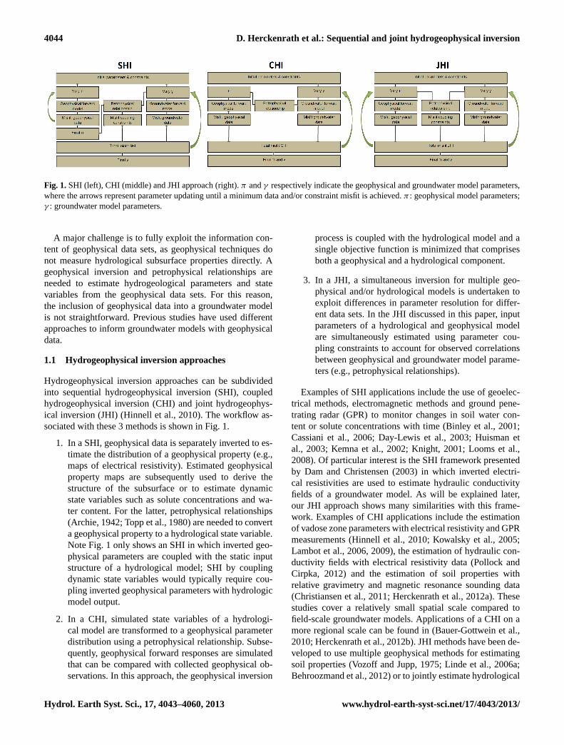
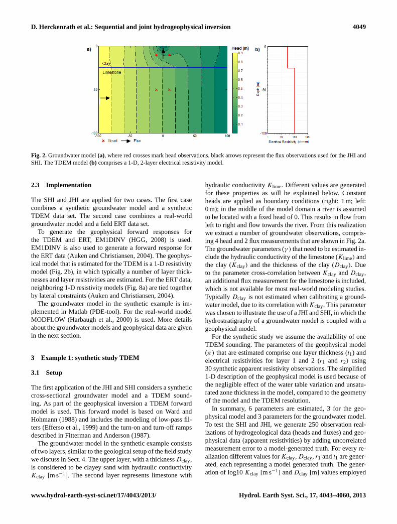
1 Fig. 2 Groundwater model (a), where red crosses mark head observations, black arrows represent the flux observations used for the 2 JHI and SHI. The TDEM model (b) comprises a 1D, 2-layer electrical resistivity model. 3 Fig. 2.Groundwater model(a), where red crosses mark head observations, black arrows represent the flux observations used for the JHI and

SHI. The TDEM model(b) comprises a 1-D, 2-layer electrical resistivity model.

2.3 Implementation

The SHI and JHI are applied for two cases. The first casecombines a synthetic groundwater model and a syntheticTDEM data set. The second case combines a real-worldgroundwater model and a field ERT data set.

To generate the geophysical forward responses forthe TDEM and ERT, EM1DINV (HGG, 2008) is used.EM1DINV is also used to generate a forward response forthe ERT data (Auken and Christiansen, 2004). The geophys-ical model that is estimated for the TDEM is a 1-D resistivitymodel (Fig. 2b), in which typically a number of layer thick-nesses and layer resistivities are estimated. For the ERT data,neighboring 1-D resistivity models (Fig. 8a) are tied togetherby lateral constraints (Auken and Christiansen, 2004).

The groundwater model in the synthetic example is im-plemented in Matlab (PDE-tool). For the real-world modelMODFLOW (Harbaugh et al., 2000) is used. More detailsabout the groundwater models and geophysical data are givenin the next section.

3 Example 1: synthetic study TDEM

3.1 Setup

The first application of the JHI and SHI considers a syntheticcross-sectional groundwater model and a TDEM sound-ing. As part of the geophysical inversion a TDEM forwardmodel is used. This forward model is based on Ward andHohmann (1988) and includes the modeling of low-pass fil-ters (Efferso et al., 1999) and the turn-on and turn-off rampsdescribed in Fitterman and Anderson (1987).

The groundwater model in the synthetic example consistsof two layers, similar to the geological setup of the field studywe discuss in Sect. 4. The upper layer, with a thicknessDclay,is considered to be clayey sand with hydraulic conductivityKclay [m s−1]. The second layer represents limestone with

hydraulic conductivityKlime. Different values are generatedfor these properties as will be explained below. Constantheads are applied as boundary conditions (right: 1 m; left:0 m); in the middle of the model domain a river is assumedto be located with a fixed head of 0. This results in flow fromleft to right and flow towards the river. From this realizationwe extract a number of groundwater observations, compris-ing 4 head and 2 flux measurements that are shown in Fig. 2a.The groundwater parameters (γ ) that need to be estimated in-clude the hydraulic conductivity of the limestone (Klime) andthe clay (Kclay) and the thickness of the clay (Dclay). Dueto the parameter cross-correlation betweenKclay andDclay,an additional flux measurement for the limestone is included,which is not available for most real-world modeling studies.Typically Dclay is not estimated when calibrating a ground-water model, due to its correlation withKclay. This parameterwas chosen to illustrate the use of a JHI and SHI, in which thehydrostratigraphy of a groundwater model is coupled with ageophysical model.

For the synthetic study we assume the availability of oneTDEM sounding. The parameters of the geophysical model(π) that are estimated comprise one layer thickness (t1) andelectrical resistivities for layer 1 and 2 (r1 and r2) using30 synthetic apparent resistivity observations. The simplified1-D description of the geophysical model is used because ofthe negligible effect of the water table variation and unsatu-rated zone thickness in the model, compared to the geometryof the model and the TDEM resolution.

In summary, 6 parameters are estimated, 3 for the geo-physical model and 3 parameters for the groundwater model.To test the SHI and JHI, we generate 250 observation real-izations of hydrogeological data (heads and fluxes) and geo-physical data (apparent resistivities) by adding uncorrelatedmeasurement error to a model-generated truth. For every re-alization different values forKclay, Dclay, r1 andt1 are gener-ated, each representing a model generated truth. The gener-ation of log10Kclay [m s−1] andDclay [m] values employed



Table 1.Model properties used in the synthetic example.

Model Property Value

Constant Head (west) [m] 1Constant Head (east) [m] 0Constant Head (river) [m] 0Error Head Measurements [m] 0.02Error Flux Measurements [ %] 30Error TDEM Measurements [ %] ca. 3 %; based on a real sounding

Table 2.Coupling constraints standard deviations,ec, used for JHI Runs 1–7.

Constraint Equation Run 1 Run 2 Run 3 Run 4 Run 5 Run 6 Run 7

Petrophysical Log10(Kclay) − Log10(r1) +6 3 2 1 0.5 0.3 0.1 0.05Geometric Dclay− t1 7 5 2 1 0.5 0.1 0.05

mean values of respectively−5 and 25 m with a standard de-viation of respectively 0.1 and 0.1 m. Subsequently values ofr1 andt1 are generated based on the equations in the secondcolumn of Table 2, including a random component with astandard deviation,ecorr, that defines the level of correlationbetween the geophysical and groundwater model parameters.

Measurement error is then added to the simulation resultsof each parameter realization, employing a standard devia-tion (eh) of ±2 cm for the head observations and±30 % forthe flux measurements. The measurement errors added to theTDEM data have a standard deviation (eg) of ca.± 3 % ofthe measurement value and are based on a real-world TDEMsounding.

The TDEM measurement error does not only reflect thestandard deviation of the data stack and includes an addi-tional error component to take into account 3-D effects andimperfect instrument specifications (e.g., filters, wave formof the applied pulses). This additional error component willtypically yield correlated measurement errors. For example,Efferso et al. (1999) provide the effect of different low passfilters on the TDEM forward response. In this research, how-ever, we do not investigate correlated errors and thus add un-correlated measurement error to the TDEM data to be con-sistent with the Gaussian assumptions of least-squares inver-sion theory (Tarantola, 2005). Different starting parametersare used for the calibration of the geophysical and ground-water model with each observation realization.

3.2 Geometric and petrophysical relationship

To perform the JHI and SHI two types of constraints are em-ployed between the groundwater and TDEM model, a geo-metric and a petrophysical constraint. Both relationships aredefined in Table 2. The geometric constraint applies to thedepth of the clay layer (Dclay) and the thickness of the firstlayer in the TDEM model (t1).

The petrophysical coupling constraint applies to the hy-draulic conductivity of the upper layer of the groundwatermodel (Kclay) and the electrical resistivity of the first layer inthe TDEM model (r1). This constraint applies a relationshipbetween the logarithmic values of hydraulic conductivity andelectrical resistivity (Niwas and de Lima, 2003; Slater, 2007).The petrophysical relationship in Table 2 was arbitrarily cho-sen, but implies a decreasing hydraulic conductivity for a de-creasing electrical resistivity, as hydraulic conductivity andelectrical resistivity decrease for increasing clay content. Atypical hydraulic conductivity for clay is 10−5 m s−1 (Fetter,1994) and 101 �m is a representative electrical resistivity(Kirsch, 2006), which results in an expected value of−6 forthe petrophysical coupling constraint. Note that this is an ex-tremely simplified relationship between hydraulic conductiv-ity and electrical resistivity.

In a first configuration of the synthetic study, we generaterealizations of “true” parameters, using a standard deviation(ecorr) of 0.01 for the petrophysical relationship and a stan-dard deviation 0.05 (ecorr) for the geometric relationship. In asecond configuration, we apply largerecorr values of respec-tively 0.1 and 0.1. As the parameter coupling in the SHI canbe very strong for well-resolved geophysical parameters, thissecond configuration is used to test whether or not the SHIresults in worse groundwater parameter estimates when cor-relation between groundwater and geophysical parameters isrelatively weak.

3.3 SHI

The SHI starts with a geophysical inversion for the TDEMdata after which the estimated electrical resistivity model,πest, is used as an observation in the calibration process ofthe groundwater model. In this caseπest comprises the es-timated values fort1 andr1, which we employ to constrainthe groundwater model parametersDclay andKclay. For theweights of these constraints (Dam and Christensen, 2003)



1 2 3 4 5 6 70

20

40

60

80

100

120

strength coupling (1: weak - 7: strong)

erro

r K

clay

[%

]

1 2 3 4 5 6 70

20

40

60

80

100


erro

r K

lime [

%]

1 2 3 4 5 6 70

10

20

30

40


erro

r D

clay

[%

]

1 2 3 4 5 6 70

5

10

15

20

25

30


erro

r r 1 [

%]

1 2 3 4 5 6 70

50

100

150

200

250


erro

r r 2 [

%]

1 2 3 4 5 6 70

10

20

30

40


erro

r t 1 [

%]

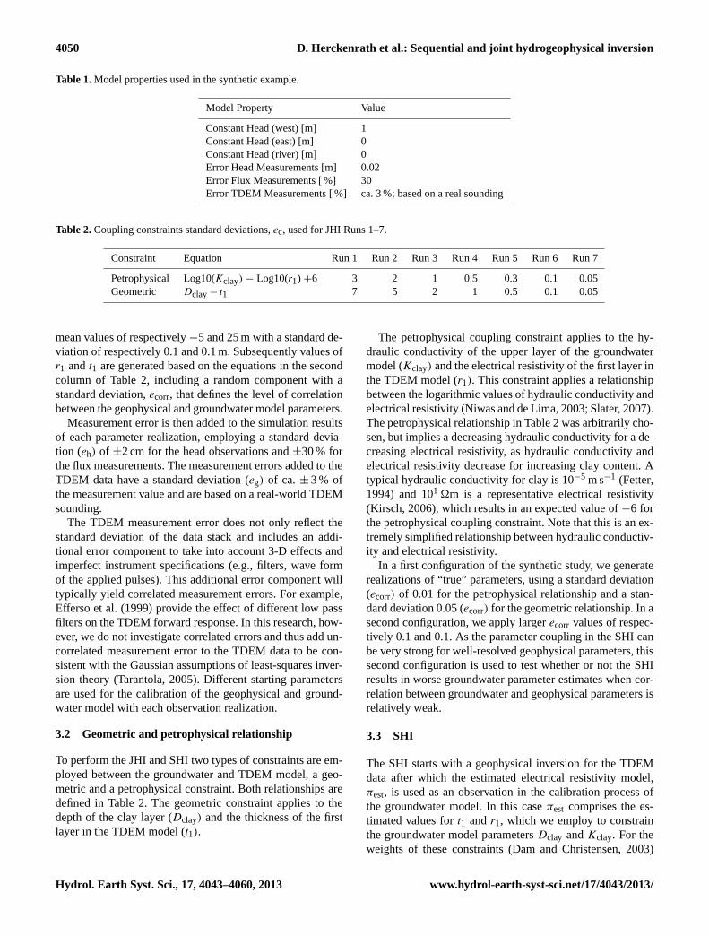
1 Fig. 3 Parameter errors for JHI Run 1-7 for 250 realizations and increasing weight for the coupling constraints (blue dashed lines). The 2 cyan lines indicate the parameter errors for the 250 SHI runs. Groundwater model parameters are shown in the upper row of figures, 3 geophysical parameters on the bottom row. Standard deviations of the JHI coupling constraints, ec, are listed in Table 2. 4 5

Fig. 3.Parameter errors for JHI Runs 1–7 for 250 realizations and increasing weight for the coupling constraints (blue dashed lines). The cyanlines indicate the parameter errors for the 250 SHI runs. Groundwater model parameters are shown in the upper row of figures, geophysicalparameters on the bottom row. Standard deviations of the JHI coupling constraints,ec, are listed in Table 2.

recommendes values of 10−2–10−1 for coupling hydraulicconductivities and well-resolved electrical resistivities andvalues of 101–102 for poorly resolved electrical resistivities.We employ values based on the posterior standard deviationof the geophysical parameters, obtained with the geophysicalinversion, to honor the resolution level of parameters inferredfrom geophysical data and constraints.

For the SHI, the second line in Eq. (13) becomes

[1 0 00 0 1

] log10(Kclay)

KlimeDclay

=

(log10(r1) − 6t1

)+ es. (25)

As Klime is not constrained with the geophysical inversionresults, its associated entries (matrixPs, Eq.13) are 0.

3.4 JHI

For the JHI we use the same type of coupling constraints forthe same geophysical and hydrological parameters. However,now the geophysical parameters are also part of the inversionand Eq. (18) is used for the coupling constraints. For thisapplication Eq. (18) becomes

[1 0 0−1 0 00 1 0 0 −1 0

]

log10(r1)

t1t2log10(Kclay)

KlimeDclay

=

(60

)+ ec, (26)

where the expected value for the geometric constraint be-tweenDclay and t1 is 0, whereas the petrophysical relation-ship between log10(Kclay) and log10(r1) is 6. The JHI is un-dertaken for varying values ofec, as defined by the valuesin Table 2. This range is comparable with the recommendedrange fores in Dam and Christensen (2003).

The value ofec reflects the strength of the coupling rela-tionship. Anec of 0.01 means the assumed error of the cou-pling relationship has a standard deviation of 0.01, markinga strong coupling relationship compared to an implementa-tion employing andec of e.g., 10. For the synthetic study theweight associated with the coupling constraints is varied, bychanging this standard deviation. Table 2 lists 7 different con-figurations of JHI (referred to as “Runs”) employing differentec values to increase the weight for the coupling relationshipbetweenDclay [m] and t1 [m] and the coupling constraintbetween log10(Kclay) [m d−1] and log10(r1) [�m]. For thepetrophysical constraintec is varied from 3 to 0.05; for thegeometric constraintec is varied from 7 to 0.05. These ranges



0 1 20

50

Cou

nt

RMSE Heads0 1 2

0

50

Cou

nt

RMSE Heads0 1 2

0

50

Cou

nt

RMSE Heads0 1 2

0

50

Cou

nt

RMSE Heads

0 1 20

50

Cou

nt

RMSE Flux0 1 2

0

50

Cou

nt

RMSE Flux0 1 2

0

50

Cou

nt

RMSE Flux0 1 2

0

50

Cou

nt

RMSE Flux

0 1 20

50

Cou

nt

RMSE Geophysics0 1 2

0

50C

ount


0

50

Cou

nt


0

50

Cou

nt

RMSE Geophysics

0 0.1 0.20

100

200

Cou

nt

RMSE Geom. con.0 0.1 0.2

0

100

200

Cou

nt


0

100

200

Cou

nt


0

100

200

Cou

nt

RMSE Geom. con.

0 0.1 0.20

100

200

Cou

nt

RMSE Petro. con.0 0.1 0.2

0

100

200

Cou

nt


0

100

200C

ount


0

100

200

Cou

nt

RMSE Petro. con.

JHI Run 1 JHI Run 4 JHI Run 7 SHI 1

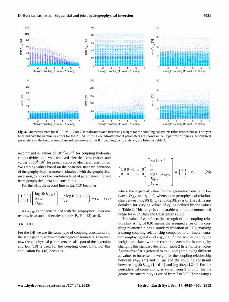
Fig. 4 Histograms of data fit for the different components of the objective function in JHI Run 1, 4 and 7. Results are for 250 2 realizations. The last column shows data fit for the SHI. 3 4

Fig. 4. Histograms of data fit for the different components of the objective function in JHI Runs 1, 4 and 7. Results are for 250 realizations.The last column shows data fit for the SHI.

were chosen to cover a JHI with weak coupling constraintsand a JHI assumingec values of similar magnitude comparedto the standard deviations,ecorr, that were used for generatingthe correlated “true” parameters.

3.5 Results

First a JHI is conducted for the groundwater and the geophys-ical model. This was done using 250 observation realizationsand different parameter starting values. 7 JHI simulations areperformed using an increasing strength of coupling betweenthe TDEM and groundwater model (Runs 1–7). To generatecorrelated “true” geophysical and groundwater model param-eters, standard deviationsecorr of 0.01 and 0.05 are respec-tively used for the petrophysical and geometric constraint.

Run 1 represents a JHI with a very small weight (i.e., largeec) for the coupling constraints representing an independentinversion in which the groundwater model is not informedwith the TDEM model and vice versa. Figure 3 shows all theparameter estimates pertaining to the JHI Run 1–7 for 250 re-alizations, expressing how well parameter estimates comparewith the “true” parameter values that were generated. Param-eter errors in Fig. 3 are given as a percentage with respect tothe “true” parameter value. For JHI Run 1 parameter errorsare up to 100 % forKclay andKlime and up to 40 % forDclay.

Geophysical parameterr1 is well-resolved and shows errorsof less than 7 %.t1 andr2 show errors of respectively 40 and200 %.

The strength of the coupling constraints is subsequentlyincreased using smaller values forec (Table 2) in JHI Runs2–7. The blue dashed lines in Fig. 3 shows how parameter es-timates react as a result of the stronger coupling constraints.A large and rapid reduction of error can be observed forKclayshowing an error decrease from 100 % to about 10 %. Esti-mates forDclay do not improve and errors remain at a valueof up to about 40 %. Geophysical parameter errors are fairlyconstant for Runs 1–7, except for a slightly increasing num-ber of realizations showing larger errors for parameterr1 andt1 in JHI Runs 6 and 7 in which the coupling constraints havethe largest weight.

Figure 4 provides the data fit for the different data typesand constraints used in the JHI in terms of root-mean squarederror (RMSE). For JHI Run 1, head, flux and TDEM dataare fitted with an RMSE of around 1 for most realizations.In JHI Run 4 coupling constraints become stronger and theRMSE for the flux and TDEM data start to increase. The headdata do not clearly show this behavior. The RMSE for thepetrophysical coupling constraint shows a decrease for JHIRuns 4 and 7, whereas the RMSE of the geometric couplingconstraint increases. The latter demonstrates the dominance



1 2 3 4 5 6 70

20

40

60

80

100

120


erro

r K

clay

[%

]

1 2 3 4 5 6 70

20

40

60

80

100


erro

r K

lime [

%]

1 2 3 4 5 6 70

10

20

30

40


erro

r D

clay

[%

]

1 2 3 4 5 6 70

5

10

15

20

25

30


erro

r r 1 [

%]

1 2 3 4 5 6 70

50

100

150

200

250


erro

r r 2 [

%]

1 2 3 4 5 6 70

10

20

30

40


erro

r t 1 [

%]

1

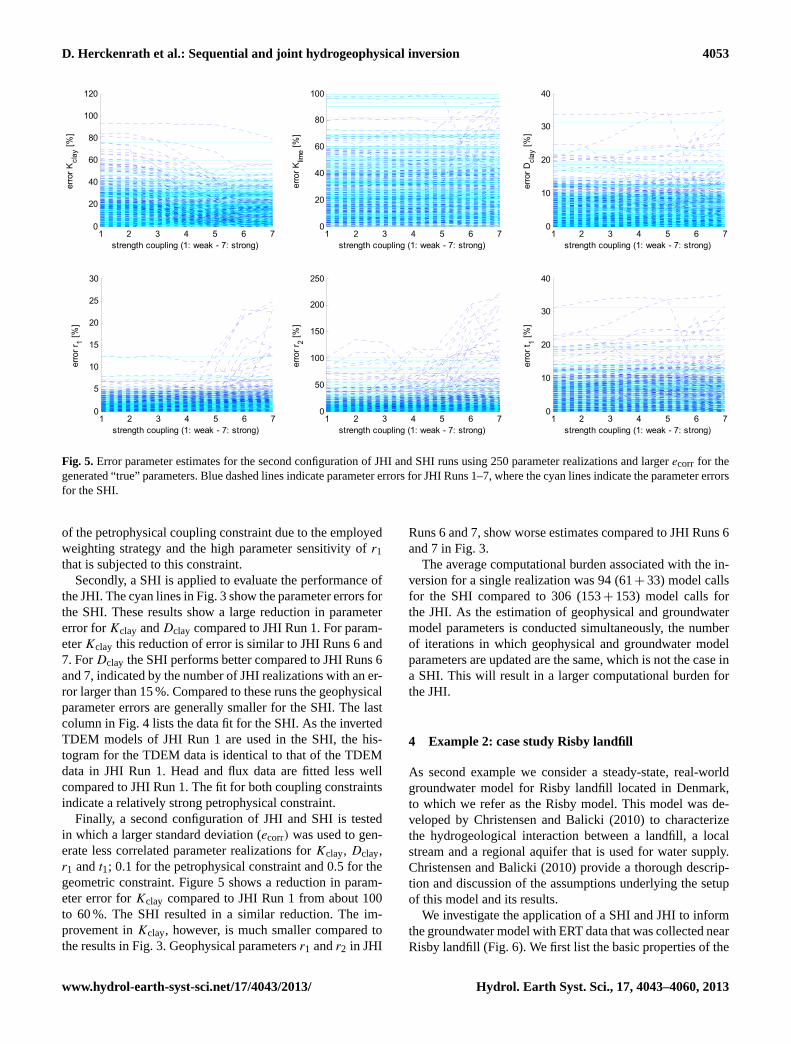
Fig. 5 Error parameter estimates for the second configuration of JHI and SHI runs using 250 parameter realizations and larger ecorr for 2 the generated “true” parameters. Blue dashed lines indicate parameter errors for JHI Run 1-7, where the cyan lines indicate the 3 parameter errors for the SHI. 4 5

Fig. 5. Error parameter estimates for the second configuration of JHI and SHI runs using 250 parameter realizations and largerecorr for thegenerated “true” parameters. Blue dashed lines indicate parameter errors for JHI Runs 1–7, where the cyan lines indicate the parameter errorsfor the SHI.

of the petrophysical coupling constraint due to the employedweighting strategy and the high parameter sensitivity ofr1that is subjected to this constraint.

Secondly, a SHI is applied to evaluate the performance ofthe JHI. The cyan lines in Fig. 3 show the parameter errors forthe SHI. These results show a large reduction in parametererror forKclay andDclay compared to JHI Run 1. For param-eterKclay this reduction of error is similar to JHI Runs 6 and7. ForDclay the SHI performs better compared to JHI Runs 6and 7, indicated by the number of JHI realizations with an er-ror larger than 15 %. Compared to these runs the geophysicalparameter errors are generally smaller for the SHI. The lastcolumn in Fig. 4 lists the data fit for the SHI. As the invertedTDEM models of JHI Run 1 are used in the SHI, the his-togram for the TDEM data is identical to that of the TDEMdata in JHI Run 1. Head and flux data are fitted less wellcompared to JHI Run 1. The fit for both coupling constraintsindicate a relatively strong petrophysical constraint.

Finally, a second configuration of JHI and SHI is testedin which a larger standard deviation (ecorr) was used to gen-erate less correlated parameter realizations forKclay, Dclay,r1 andt1; 0.1 for the petrophysical constraint and 0.5 for thegeometric constraint. Figure 5 shows a reduction in param-eter error forKclay compared to JHI Run 1 from about 100to 60 %. The SHI resulted in a similar reduction. The im-provement inKclay, however, is much smaller compared tothe results in Fig. 3. Geophysical parametersr1 andr2 in JHI

Runs 6 and 7, show worse estimates compared to JHI Runs 6and 7 in Fig. 3.

The average computational burden associated with the in-version for a single realization was 94 (61+ 33) model callsfor the SHI compared to 306 (153+ 153) model calls forthe JHI. As the estimation of geophysical and groundwatermodel parameters is conducted simultaneously, the numberof iterations in which geophysical and groundwater modelparameters are updated are the same, which is not the case ina SHI. This will result in a larger computational burden forthe JHI.

4 Example 2: case study Risby landfill

As second example we consider a steady-state, real-worldgroundwater model for Risby landfill located in Denmark,to which we refer as the Risby model. This model was de-veloped by Christensen and Balicki (2010) to characterizethe hydrogeological interaction between a landfill, a localstream and a regional aquifer that is used for water supply.Christensen and Balicki (2010) provide a thorough descrip-tion and discussion of the assumptions underlying the setupof this model and its results.

We investigate the application of a SHI and JHI to informthe groundwater model with ERT data that was collected nearRisby landfill (Fig. 6). We first list the basic properties of the



1

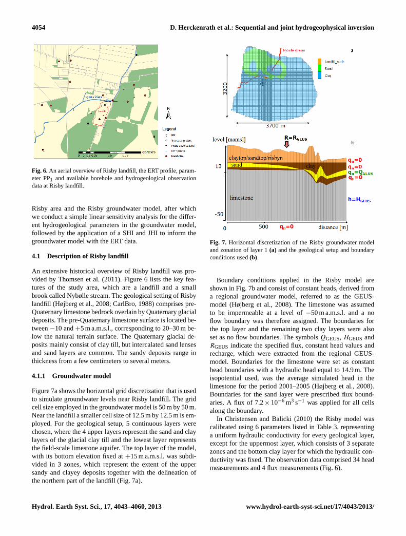
Fig. 6 An aerial overview of Risby landfill, the ERT profile, parameter PP1 and available boreholes and hydrogeological observation 2 data at Risby landfill. 3 Fig. 6.An aerial overview of Risby landfill, the ERT profile, param-eter PP1 and available borehole and hydrogeological observationdata at Risby landfill.

Risby area and the Risby groundwater model, after whichwe conduct a simple linear sensitivity analysis for the differ-ent hydrogeological parameters in the groundwater model,followed by the application of a SHI and JHI to inform thegroundwater model with the ERT data.

4.1 Description of Risby landfill

An extensive historical overview of Risby landfill was pro-vided by Thomsen et al. (2011). Figure 6 lists the key fea-tures of the study area, which are a landfill and a smallbrook called Nybølle stream. The geological setting of Risbylandfill (Højberg et al., 2008; CarlBro, 1988) comprises pre-Quaternary limestone bedrock overlain by Quaternary glacialdeposits. The pre-Quaternary limestone surface is located be-tween−10 and+5 m a.m.s.l., corresponding to 20–30 m be-low the natural terrain surface. The Quaternary glacial de-posits mainly consist of clay till, but intercalated sand lensesand sand layers are common. The sandy deposits range inthickness from a few centimeters to several meters.

4.1.1 Groundwater model

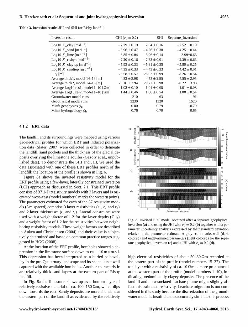
Figure 7a shows the horizontal grid discretization that is usedto simulate groundwater levels near Risby landfill. The gridcell size employed in the groundwater model is 50 m by 50 m.Near the landfill a smaller cell size of 12.5 m by 12.5 m is em-ployed. For the geological setup, 5 continuous layers werechosen, where the 4 upper layers represent the sand and claylayers of the glacial clay till and the lowest layer representsthe field-scale limestone aquifer. The top layer of the model,with its bottom elevation fixed at+15 m a.m.s.l. was subdi-vided in 3 zones, which represent the extent of the uppersandy and clayey deposits together with the delineation ofthe northern part of the landfill (Fig. 7a).

1 2 Fig. 7 Horizontal discretization of the Risby groundwater model and zonation of layer 1 (a) and the geological setup and boundary 3 conditions used (b). 4

Fig. 7. Horizontal discretization of the Risby groundwater modeland zonation of layer 1(a) and the geological setup and boundaryconditions used(b).

Boundary conditions applied in the Risby model areshown in Fig. 7b and consist of constant heads, derived froma regional groundwater model, referred to as the GEUS-model (Højberg et al., 2008). The limestone was assumedto be impermeable at a level of−50 m a.m.s.l. and a noflow boundary was therefore assigned. The boundaries forthe top layer and the remaining two clay layers were alsoset as no flow boundaries. The symbolsQGEUS, HGEUS andRGEUS indicate the specified flux, constant head values andrecharge, which were extracted from the regional GEUS-model. Boundaries for the limestone were set as constanthead boundaries with a hydraulic head equal to 14.9 m. Theisopotential used, was the average simulated head in thelimestone for the period 2001–2005 (Højberg et al., 2008).Boundaries for the sand layer were prescribed flux bound-aries. A flux of 7.2× 10−6 m3 s−1 was applied for all cellsalong the boundary.

In Christensen and Balicki (2010) the Risby model wascalibrated using 6 parameters listed in Table 3, representinga uniform hydraulic conductivity for every geological layer,except for the uppermost layer, which consists of 3 separatezones and the bottom clay layer for which the hydraulic con-ductivity was fixed. The observation data comprised 34 headmeasurements and 4 flux measurements (Fig. 6).



Table 3. Inversion results JHI and SHI for Risby landfill.

Inversion result CHI (ec = 0.2) SHI Separate_Inversion

Log10K_clay [m d−1] −7.79± 0.19 7.54± 0.16 −7.52± 0.19Log10K_sand [m d−1] −3.96± 0.47 −4.26± 0.38 −4.25± 0.44Log10K_lime [m d−1] −3.85± 0.04 −3.96± 0.14 −3.99±0.66Log10K_risbyn [m d−1] −2.20± 0.16 −2.33± 0.01 −2.39± 0.63Log10K_claytop [m d−1] −5.93± 0.33 −5.81± 0.35 −5.80± 0.25Log10K_sandtop [m d−1] −4.35± 0.33 −4.43± 0.33 −4.42± 0.01PP1 [m] 26.58± 0.57 28.03± 0.99 28.26± 0.54Average thick1, model 14–16 [m] 4.53± 3.08 4.55± 2.95 4.55± 2.95Average thick2, model 14–16 [m] 20.16± 3.94 20.22± 3.98 20.22± 3.98Average Log10 res1, model 1–10 [�m] 1.02± 0.10 1.01± 0.08 1.01± 0.08Average Log10 res2, model 1–10 [�m] 1.44± 0.46 1.88± 0.54 1.88± 0.54Groundwater model runs 210 63 91Geophysical model runs 3230 1520 1520Misfit geophysicsφg 0.80 0.79 0.79Misfit hydrogeologyφh 0.76 0.70 0.65

4.1.2 ERT data

The landfill and its surroundings were mapped using variousgeoelectrical profiles for which ERT and induced polariza-tion data (Slater, 2007) were collected in order to delineatethe landfill, sand pockets and the thickness of the glacial de-posits overlying the limestone aquifer (Gazoty et al., unpub-lished data). To demonstrate the SHI and JHI, we used thedata associated with one of these ERT profiles north of thelandfill; the location of the profile is shown in Fig. 6.

Figure 8a shows the inverted resistivity model for theERT profile using a few-layer, laterally constrained inversion(LCI) approach as discussed in Sect. 2.1. This ERT profileconsists of 37 1-D resistivity models with 3 layers and is ori-entated west–east (model number 0 marks the western point).The parameters estimated for each of the 37 resistivity mod-els (5 m spaced) comprise 3 layer resistivities (r1, r2 andr3)

and 2 layer thicknesses (t1 andt2). Lateral constraints wereused with a weight factor of 1.2 for the layer depths (CRh)

and a weight factor of 1.2 for the resistivities between neigh-boring resistivity models. These weight factors are describedin Auken and Christiansen (2004) and their value is subjec-tively determined and based on common practice ranges sug-gested in HGG (2008).

At the location of the ERT profile, boreholes showed a de-pression in the limestone surface down to ca.−10 m a.m.s.l.This depression has been interpreted as a buried paleoval-ley in the pre-Quaternary landscape and its shape is not wellcaptured with the available boreholes. Another characteristicare relatively thick sand layers at the eastern part of Risbylandfill.

In Fig. 8a the limestone shows up as a bottom layer ofrelatively resistive material of ca. 100–150�m, which dipsdown towards the east. Sandy deposits are more abundant atthe eastern part of the landfill as evidenced by the relatively

-40

-20

0

20

Ele

vatio

n [m

am

sl]

r1

r2

r3

t1

t2

-40

-20

0

20

Ele

vatio

n [m

am

sl]

0

5

10

15

20

25

30

35

40

45

50

5 10 15 20 25 30 35

r1

r2

r3

t1

t2

Resistivity model number

20

40

60

80

100

120

140a)

Ana

lysi

s [%

]E

lect

rica

l res

istiv

ity [o

hm

m]

b)

c)

d)

1

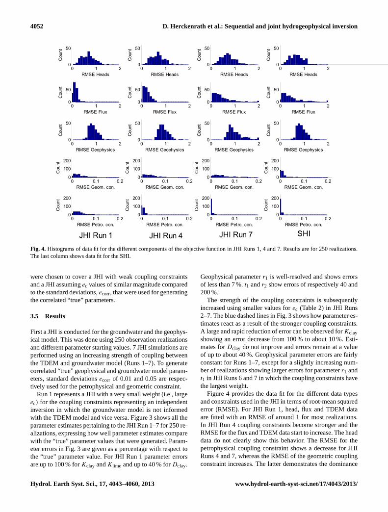
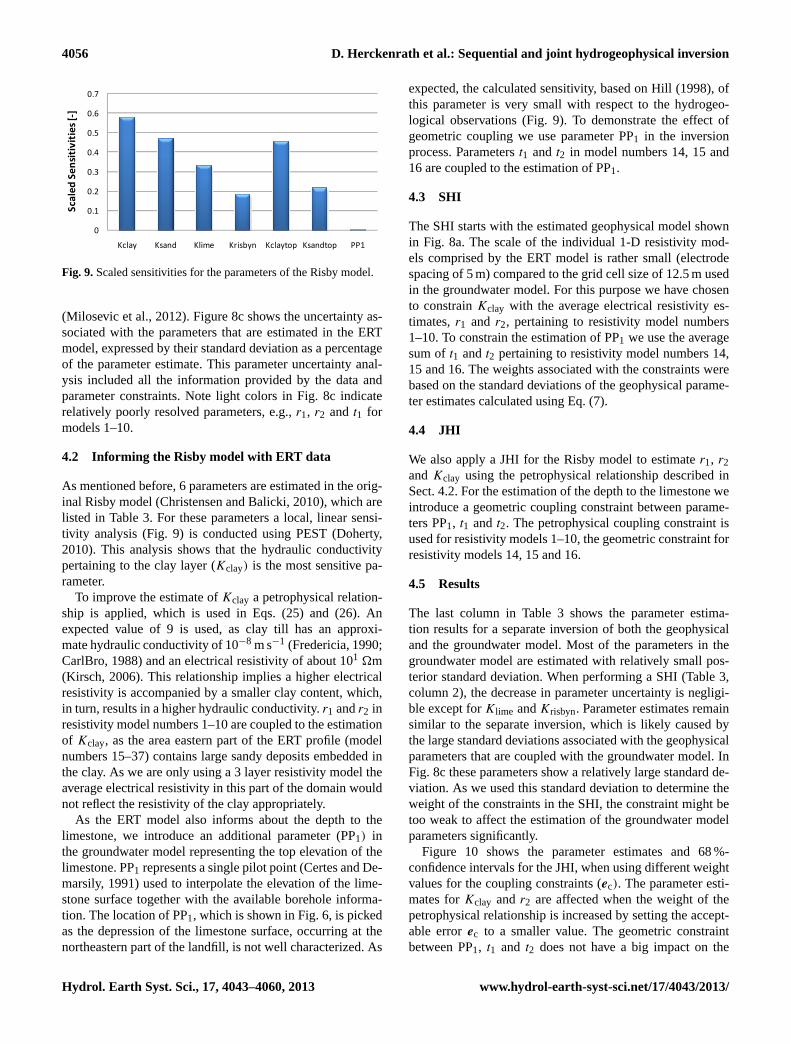
Fig. 8 Inverted ERT model obtained after a separate geophysical inversion (a) and using the JHI with ec=0.2 (b) together with a 2 parameter uncertainty analysis expressed by their standard deviation relative to the parameter estimate. A gray scale marks well (dark 3 colored) and undetermined parameters (light colored) for the separate geophysical inversion (c) and a JHI with ec=0.2 (d). 4 5

Fig. 8. Inverted ERT model obtained after a separate geophysicalinversion(a) and using the JHI withec = 0.2(b) together with a pa-rameter uncertainty analysis expressed by their standard deviationrelative to the parameter estimate. A gray scale marks well (darkcolored) and undetermined parameters (light colored) for the sepa-rate geophysical inversion(c) and a JHI withec = 0.2 (d).

high electrical resistivities of about 50–80�m recorded atthe eastern part of the profile (model numbers 15–37). Thetop layer with a resistivity of ca. 10�m is more pronouncedat the western part of the profile (model numbers 1–10), in-dicating predominantly clayey deposits. The presence of thelandfill and an associated leachate plume might slightly af-fect this estimated resistivity. Leachate migration is not con-sidered in this study because the discretization of the ground-water model is insufficient to accurately simulate this process



0

0.1

0.2

0.3

0.4

0.5

0.6

0.7

Kclay Ksand Klime Krisbyn Kclaytop Ksandtop PP1

Scaled

Sen

sitivities [‐]

1

Fig. 9 Scaled Sensitivities for the parameters of the Risby model. 2 Fig. 9.Scaled sensitivities for the parameters of the Risby model.

(Milosevic et al., 2012). Figure 8c shows the uncertainty as-sociated with the parameters that are estimated in the ERTmodel, expressed by their standard deviation as a percentageof the parameter estimate. This parameter uncertainty anal-ysis included all the information provided by the data andparameter constraints. Note light colors in Fig. 8c indicaterelatively poorly resolved parameters, e.g.,r1, r2 and t1 formodels 1–10.

4.2 Informing the Risby model with ERT data

As mentioned before, 6 parameters are estimated in the orig-inal Risby model (Christensen and Balicki, 2010), which arelisted in Table 3. For these parameters a local, linear sensi-tivity analysis (Fig. 9) is conducted using PEST (Doherty,2010). This analysis shows that the hydraulic conductivitypertaining to the clay layer (Kclay) is the most sensitive pa-rameter.

To improve the estimate ofKclay a petrophysical relation-ship is applied, which is used in Eqs. (25) and (26). Anexpected value of 9 is used, as clay till has an approxi-mate hydraulic conductivity of 10−8 m s−1 (Fredericia, 1990;CarlBro, 1988) and an electrical resistivity of about 101 �m(Kirsch, 2006). This relationship implies a higher electricalresistivity is accompanied by a smaller clay content, which,in turn, results in a higher hydraulic conductivity.r1 andr2 inresistivity model numbers 1–10 are coupled to the estimationof Kclay, as the area eastern part of the ERT profile (modelnumbers 15–37) contains large sandy deposits embedded inthe clay. As we are only using a 3 layer resistivity model theaverage electrical resistivity in this part of the domain wouldnot reflect the resistivity of the clay appropriately.

As the ERT model also informs about the depth to thelimestone, we introduce an additional parameter (PP1) inthe groundwater model representing the top elevation of thelimestone. PP1 represents a single pilot point (Certes and De-marsily, 1991) used to interpolate the elevation of the lime-stone surface together with the available borehole informa-tion. The location of PP1, which is shown in Fig. 6, is pickedas the depression of the limestone surface, occurring at thenortheastern part of the landfill, is not well characterized. As

expected, the calculated sensitivity, based on Hill (1998), ofthis parameter is very small with respect to the hydrogeo-logical observations (Fig. 9). To demonstrate the effect ofgeometric coupling we use parameter PP1 in the inversionprocess. Parameterst1 and t2 in model numbers 14, 15 and16 are coupled to the estimation of PP1.

4.3 SHI

The SHI starts with the estimated geophysical model shownin Fig. 8a. The scale of the individual 1-D resistivity mod-els comprised by the ERT model is rather small (electrodespacing of 5 m) compared to the grid cell size of 12.5 m usedin the groundwater model. For this purpose we have chosento constrainKclay with the average electrical resistivity es-timates,r1 and r2, pertaining to resistivity model numbers1–10. To constrain the estimation of PP1 we use the averagesum oft1 andt2 pertaining to resistivity model numbers 14,15 and 16. The weights associated with the constraints werebased on the standard deviations of the geophysical parame-ter estimates calculated using Eq. (7).

4.4 JHI

We also apply a JHI for the Risby model to estimater1, r2andKclay using the petrophysical relationship described inSect. 4.2. For the estimation of the depth to the limestone weintroduce a geometric coupling constraint between parame-ters PP1, t1 and t2. The petrophysical coupling constraint isused for resistivity models 1–10, the geometric constraint forresistivity models 14, 15 and 16.

4.5 Results

The last column in Table 3 shows the parameter estima-tion results for a separate inversion of both the geophysicaland the groundwater model. Most of the parameters in thegroundwater model are estimated with relatively small pos-terior standard deviation. When performing a SHI (Table 3,column 2), the decrease in parameter uncertainty is negligi-ble except forKlime andKrisbyn. Parameter estimates remainsimilar to the separate inversion, which is likely caused bythe large standard deviations associated with the geophysicalparameters that are coupled with the groundwater model. InFig. 8c these parameters show a relatively large standard de-viation. As we used this standard deviation to determine theweight of the constraints in the SHI, the constraint might betoo weak to affect the estimation of the groundwater modelparameters significantly.

Figure 10 shows the parameter estimates and 68 %-confidence intervals for the JHI, when using different weightvalues for the coupling constraints (ec). The parameter esti-mates forKclay andr2 are affected when the weight of thepetrophysical relationship is increased by setting the accept-able errorec to a smaller value. The geometric constraintbetween PP1, t1 and t2 does not have a big impact on the



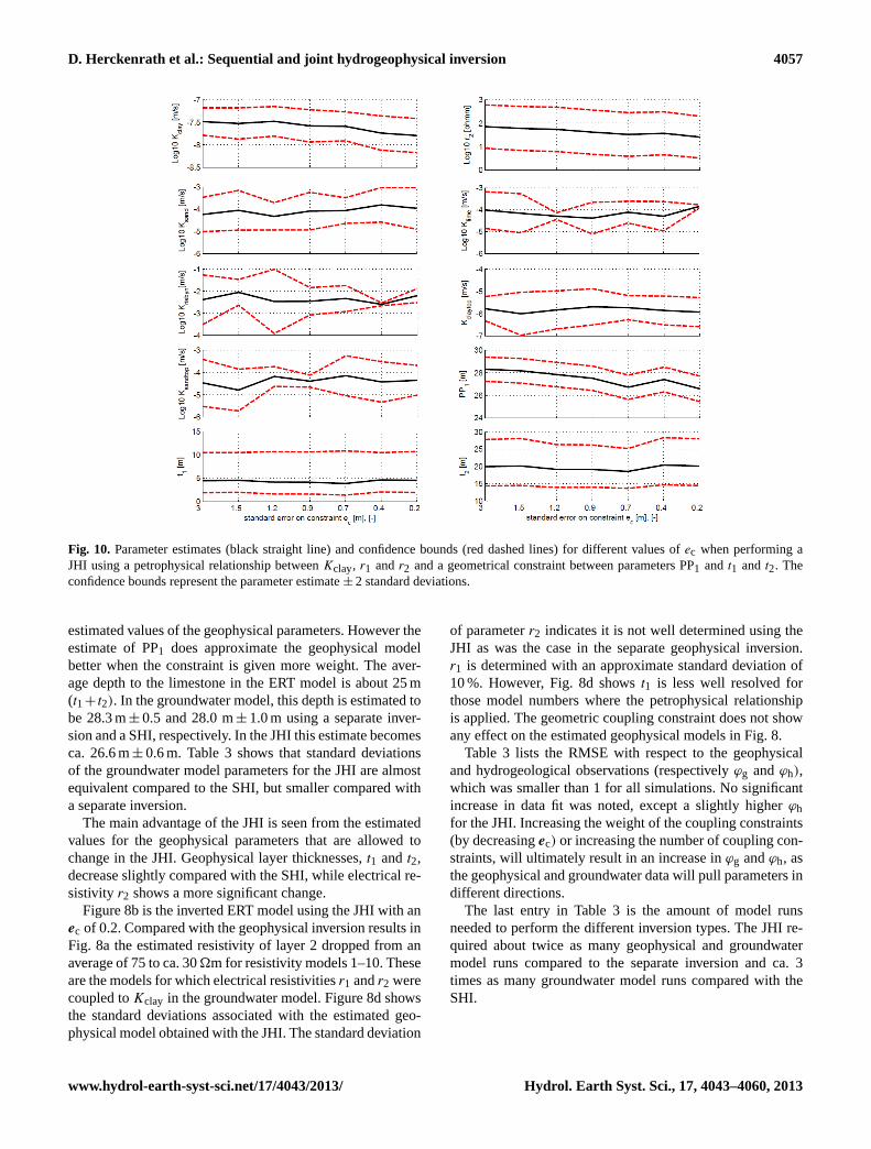
1 Fig. 10 Parameter estimates (black straight line) and confidence bounds (red dashed lines) for different values of ec when performing a 2 JHI using a petrophysical relationship between Kclay, r1 and r2 and a geometrical constraint between parameters PP1 and t1 and t2. The 3 confidence bounds represent the parameter estimate ± 2 standard deviations. 4 5

6

Fig. 10. Parameter estimates (black straight line) and confidence bounds (red dashed lines) for different values ofec when performing aJHI using a petrophysical relationship betweenKclay, r1 andr2 and a geometrical constraint between parameters PP1 and t1 and t2. Theconfidence bounds represent the parameter estimate± 2 standard deviations.

estimated values of the geophysical parameters. However theestimate of PP1 does approximate the geophysical modelbetter when the constraint is given more weight. The aver-age depth to the limestone in the ERT model is about 25 m(t1+ t2). In the groundwater model, this depth is estimated tobe 28.3 m± 0.5 and 28.0 m± 1.0 m using a separate inver-sion and a SHI, respectively. In the JHI this estimate becomesca. 26.6 m± 0.6 m. Table 3 shows that standard deviationsof the groundwater model parameters for the JHI are almostequivalent compared to the SHI, but smaller compared witha separate inversion.

The main advantage of the JHI is seen from the estimatedvalues for the geophysical parameters that are allowed tochange in the JHI. Geophysical layer thicknesses,t1 andt2,decrease slightly compared with the SHI, while electrical re-sistivity r2 shows a more significant change.

Figure 8b is the inverted ERT model using the JHI with anec of 0.2. Compared with the geophysical inversion results inFig. 8a the estimated resistivity of layer 2 dropped from anaverage of 75 to ca. 30�m for resistivity models 1–10. Theseare the models for which electrical resistivitiesr1 andr2 werecoupled toKclay in the groundwater model. Figure 8d showsthe standard deviations associated with the estimated geo-physical model obtained with the JHI. The standard deviation

of parameterr2 indicates it is not well determined using theJHI as was the case in the separate geophysical inversion.r1 is determined with an approximate standard deviation of10 %. However, Fig. 8d showst1 is less well resolved forthose model numbers where the petrophysical relationshipis applied. The geometric coupling constraint does not showany effect on the estimated geophysical models in Fig. 8.

Table 3 lists the RMSE with respect to the geophysicaland hydrogeological observations (respectivelyϕg andϕh),which was smaller than 1 for all simulations. No significantincrease in data fit was noted, except a slightly higherϕhfor the JHI. Increasing the weight of the coupling constraints(by decreasingec) or increasing the number of coupling con-straints, will ultimately result in an increase inϕg andϕh, asthe geophysical and groundwater data will pull parameters indifferent directions.

The last entry in Table 3 is the amount of model runsneeded to perform the different inversion types. The JHI re-quired about twice as many geophysical and groundwatermodel runs compared to the separate inversion and ca. 3times as many groundwater model runs compared with theSHI.



5 Discussion and conclusions

This study tested a SHI and a new type of JHI for a ground-water model and different types of geophysical data. TheJHI estimated geophysical and groundwater parameters si-multaneously, employing coupling constraints acting as ad-ditional regularization terms to exploit potential correlationbetween geophysical and hydrogeological properties that canbe based on established petrophysical relationships. The SHIemployed similar coupling constraints, but included an inde-pendent geophysical inversion. The weight of the SHI cou-pling constraints was based on geophysical parameter reso-lution.

Both the SHI and JHI approaches can provide consistentinversion frameworks and offer a high level of flexibilitywhen coupling groundwater and geophysical models because

1. only selected geophysical model parameters can becoupled to groundwater model parameters,

2. confidence associated with the hydrological interpre-tation of a geophysical model can be tuned using dif-ferent weights for the employed coupling constraints,

3. scale issues can be overcome by coupling several geo-physical parameters to hydrological parameters or viceversa,

4. SHI and JHI can be applied for various combinationsof geophysical methods and groundwater models, and

5. SHI and JHI can be used with other types of optimiza-tion methods (e.g., Markov–Chain Monte Carlo meth-ods) by adding an additional coupling constraint com-ponent to the objective function that is minimized.

Furthermore, the JHI and SHI are consistent with state-of-the-art inversion techniques used for groundwater models,resistivity and airborne electromagnetic data.

For a synthetic study, comprising a cross-sectional ground-water model and TDEM data, a JHI and SHI resulted in im-proved parameter estimates and a reduction in parameter un-certainty in comparison with a groundwater model that isnot informed with TDEM data. Groundwater parameter esti-mates using a JHI did not improve compared with a SHI andresulted in slightly worse parameter estimates for the geo-physical model when using large weights for the couplingconstraints. A second configuration of the synthetic study,incorporating lower quality (petro)physical relationships be-tween geophysical and groundwater parameters resulted indecreasing performances for both the SHI and JHI. The SHIperformed slightly better compared to the JHI based on thegeophysical parameter estimates and geophysical data mis-fit. In contrast to the JHI, the SHI overestimated the levelof correlation between geophysical and groundwater param-eters. To avoid overestimating model coupling strength ina SHI (which can result in an underestimation of parame-ter uncertainty), weighting strategies for parameter coupling

constraints should be based on that element (parameter res-olution or petrophysical relationship) that incorporates thelargest error.

For the case of a real-world, field-scale groundwater modeland an ERT section, parameter uncertainty was significantlydecreased for two parameters in the groundwater model us-ing both a JHI and SHI. The JHI resulted in different param-eter estimates for both the groundwater and the geophysicalmodel, honoring the imposed coupling constraints. Parame-ter uncertainty was not reduced in comparison with a SHI.

For the cases investigated in this paper the SHI proves tobe more useful based on analyses of parameter estimates anddata fit. In addition, the JHI requires a 2–3 times larger com-putational burden and is relatively difficult to implement. TheJHI might still be useful when groundwater and geophysicalmodels can mutually benefit from differences in parameterresolution. For coupling geophysical models with field-scaleor regional groundwater models, such situation is not likelyto occur as the groundwater models are relatively more proneto conceptual errors and limited observation data. Finally,when planning hydrogeophysical surveys and modeling, pa-rameter sensitivity studies are of crucial importance to ex-plore parameters that need to be determined, given targetedgroundwater model predictions, and to determine whetherparameter resolution in geophysical models provides oppor-tunities to constrain these parameters.

Acknowledgements.This work was conducted at the TechnicalUniversity of Denmark and supported by the Danish Agency forScience Technology and Innovation funded project RiskPoint– Assessing the risks posed by point source contamination togroundwater and surface water resources under grant number09-063216. We also like to thank Monika Balicki and MetteChristensen for the main development of the Risby groundwatermodel and Aurélie Gazoty for the ERT data collection. Finally, wewant to thank three anonymous reviewers for sharpening a previousversion of this paper.

Edited by: G. Fogg

References

Archie, G. E.: The electrical resistivity log as an aid in determin-ing some reservoir characteristics, Transactions of the AmericanInstitute of Mining and Metallurgical Engineers, 146 154–161,1942.

Auken, E. and Christiansen, A. V.: Layered and laterally con-strained 2d inversion of resistivity data, Geophysics, 69, 752–761, doi:10.1190/1.1759461, 2004.

Bauer-Gottwein, P., Gondwe, B. N., Christiansen, L., Herckenrath,D., Kgotlhang, L., and Zimmermann, S.: Hydrogeophysical ex-ploration of three-dimensional salinity anomalies with the time-domain electromagnetic method (tdem), J. Hydrol., 380, 318–329, doi:10.1016/j.jhydrol.2009.11.007, 2010.

Behroozmand, A. A., Auken, E., Fiandaca, G., and Christiansen,A. V.: Improvement in mrs parameter estimation by joint and


http://dx.doi.org/10.1190/1.1759461

http://dx.doi.org/10.1016/j.jhydrol.2009.11.007


laterally constrained inversion of mrs and tem data, Geophysics,77, WB191-WB200, doi:10.1190/geo2011-0404.1, 2012.

Binley, A., Winship, P., Middleton, R., Pokar, M., and West, J.:High-resolution characterization of vadose zone dynamics usingcross-borehole radar, Water Resour. Res., 37, 2639–2652, 2001.

Burschil, T., Scheer, W., Kirsch, R., and Wiederhold, H.: Compil-ing geophysical and geological information into a 3-D model ofthe glacially-affected island of Föhr, Hydrol. Earth Syst. Sci., 16,3485–3498, doi:10.5194/hess-16-3485-2012, 2012.

CarlBro, A. S.: Afsluttende fase 2 – undersøgelse på risby losse-plads, københavns amtskommune, copenhagen, denmark, 1988.

Carrera, J., Hidalgo, J. J., Slooten, L. J., and Vazquez-Sune,E.: Computational and conceptual issues in the calibrationof seawater intrusion models, Hydrogeol. J., 18, 131–145,doi:10.1007/s10040-009-0524-1, 2010.

Cassiani, G., Bruno, V., Villa, A., Fusi, N., and Binley, A. M.:A saline trace test monitored via time-lapse surface electri-cal resistivity tomography, J. Appl. Geophys., 59, 244–259,doi:10.1016/j.jappgeo2005.10.007, 2006.

Certes, C. and Demarsily, G.: Application of the pilot point methodto the identification of aquifer transmissivities, Adv. Water Re-sour., 14, 284–300, 1991.

Chen, J., Hubbard, S., Peterson, J., Williams, K., Fienen, M.,Jardine, P., and Watson, D.: Development of a joint hydro-geophysical inversion approach and application to a contam-inated fractured aquifer, Water Resour. Res., 42, W06425,doi:10.1029/2005wr004694, 2006.

Christensen, M. and Balicki, M.: Hydrogeological characterizationand numerical modeling of groundwater-surface water interac-tion at risby landfill, Master’s Thesis, Environmental Engineer-ing, Technical University of Denmark, Kgs. Lyngby, 2010.

Christiansen, L., Binning, P. J., Rosbjerg, D., Andersen, O. B.,and Bauer-Gottwein, P.: Using time-lapse gravity for groundwa-ter model calibration: An application to alluvial aquifer storage,Water Resour. Res., 47, W06503, doi:10.1029/2010wr009859,2011.

Dam, D. and Christensen, S.: Including geophysical data in groundwater model inverse calibration, Ground Water, 41, 178–189,doi:10.1111/j.1745-6584.2003.tb02581.x, 2003.

Day-Lewis, F. D., Lane, J. W., Harris, J. M., and Gorelick, S. M.:Time-lapse imaging of saline-tracer transport in fractured rockusing difference-attenuation radar tomography, Water Resour.Res., 39, 1290, doi:10.1029/2002wr001722, 2003.

Day-Lewis, F. D., Singha, K., and Binley, A. M.: Applying petro-physical models to radar travel time and electrical resistivity to-mograms: Resolution-dependent limitations, J. Geophys. Res.-Solid Earth, 110, B08206, doi:10.1029/2004jb003569, 2005.

Doherty, J.: Pest: Model-independent parameter estimation, in: Wa-termark Numerical Computing, Brisbane, Queensland, Australia,2010.

Doherty, J. and Johnston, J. M.: Methodologies for calibra-tion and predictive analysis of a watershed model, J. Amer-ican Water Resour. Assoc., 39, 251–265, doi:10.1111/j.1752-1688.2003.tb04381.x, 2003.

Efferso, F., Auken, E., and Sorensen, K. I.: Inversion of band-limited tem responses, Geophys. Prospect., 47, 551–564,doi:10.1046/j.1365-2478.1999.00135.x, 1999.

Faneca Sànchez, M., Gunnink, J. L., van Baaren, E. S., OudeEssink, G. H. P., Siemon, B., Auken, E., Elderhorst, W., and

de Louw, P. G. B.: Modelling climate change effects on aDutch coastal groundwater system using airborne electromag-netic measurements, Hydrol. Earth Syst. Sci., 16, 4499–4516,doi:10.5194/hess-16-4499-2012, 2012.

Fetter, C. W.: Applied hydrogeology, 3rd Edn., Prentice-Hall, NewJersey, USA, 1994.

Fitterman, D. V. and Anderson, W. L.: Effect of transmitter turn-off time on transient soundings, Geoexploration, 24, 131–146,doi:10.1016/0016-7142(87)90087-1, 1987.

Fitzpatrick, A., Cahill, K., Munday, T., and Berens, V.: Inform-ing the hydrogeology of coffin bay, south australia, through theconstrained inversion of tempest aem data, CSIRO Water for aHealthy Country National Research Flagship, 2009.

Fredericia, J.: Saturated hydraulic conductivity of clayey tills andthe role of fractures, Nordic Hydrology, 21, 119–132, 1990.

Harbaugh, A. W., Banta, E. R., Hill, M. C., and McDonald, M.G.: Modflow 2000, the U.S. Geological survey modular ground-water model – user guide to modularisation concepts and thegroundwater flow process, US Geological Survey, Reston, 130pp., 2000.

Herckenrath, D., Auken, E., Christiansen, L., Behroozmand, A.A., and Bauer-Gottwein, P.: Coupled hydrogeophysical in-version using time-lapse magnetic resonance sounding andtime-lapse gravity data for hydraulic aquifer testing: Willit work in practice?, Water Resour. Res., 48, W01539,doi:10.1029/2011wr010411, 2012a.

Herckenrath, D., Odlum, N., Nenna, V., Knight, R., Auken,E., and Bauer-Gottwein, P.: Calibrating a salt water intrusionmodel with time-domain electromagnetic data, Ground Water,doi:10.1111/j.1745-6584.2012.00974.x, 2012b.

HGG: Manual for the inversion program em1dinv, version 5.2, De-partment of Earth Sciences, University of Aarhus, Denmark,2008.

Hill, M. C.: Methods and guidelines for effective model calibrationUS Geological Survey, 1998.

Hinnell, A. C., Ferre, T. P. A., Vrugt, J. A., Huisman, J. A., Moy-sey, S., Rings, J., and Kowalsky, M. B.: Improved extraction ofhydrologic information from geophysical data through coupledhydrogeophysical inversion, Water Resour. Res., 46, W00d40,doi:10.1029/2008wr007060, 2010.

Højberg, A. L., Troldborg, L., Nyegaard, P., Ondracek, M., Stisen,S., Christensen, B. S. B., and Nørgaard, A.: National vandres-source model – sjælland, lolland, falster og møn, GEUS, Copen-hagen, Denmark, 2008.

Hubbard, S. S. and Rubin, Y.: Hydrogeological parameter es-timation using geophysical data: A review of selected tech-niques, J. Contaminant Hydrol., 45, 3–34, doi:10.1016/s0169-7722(00)00117-0, 2000.

Huisman, J. A., Hubbard, S. S., Redman, J. D., and Annan, A. P.:Measuring soil water content with ground penetrating radar: Areview, Vadose Zone J., 2, 476–491, 2003.

Hyndman, D. W. and Gorelick, S. M.: Estimating lithologic andtransport properties in three dimensions using seismic and tracerdata: The kesterson aquifer, Water Resour. Res., 32, 2659–2670,doi:10.1029/96wr01269, 1996.

Kemna, A., Vanderborght, J., Kulessa, B., and Vereecken, H.:Imaging and characterisation of subsurface solute transport us-ing electrical resistivity tomography (ert) and equivalent trans-


http://dx.doi.org/10.1190/geo2011-0404.1

http://dx.doi.org/10.5194/hess-16-3485-2012

http://dx.doi.org/10.1007/s10040-009-0524-1

http://dx.doi.org/10.1016/j.jappgeo2005.10.007

http://dx.doi.org/10.1029/2005wr004694

http://dx.doi.org/10.1029/2010wr009859

http://dx.doi.org/10.1111/j.1745-6584.2003.tb02581.x

http://dx.doi.org/10.1029/2002wr001722

http://dx.doi.org/10.1029/2004jb003569



http://dx.doi.org/10.1046/j.1365-2478.1999.00135.x

http://dx.doi.org/10.5194/hess-16-4499-2012

http://dx.doi.org/10.1016/0016-7142(87)90087-1

http://dx.doi.org/10.1029/2011wr010411

http://dx.doi.org/10.1111/j.1745-6584.2012.00974.x

http://dx.doi.org/10.1029/2008wr007060

http://dx.doi.org/10.1016/s0169-7722(00)00117-0

http://dx.doi.org/10.1016/s0169-7722(00)00117-0

http://dx.doi.org/10.1029/96wr01269


port models, J. Hydrol., 267, 125–146, doi:10.1016/s0022-1694(02)00145-2, 2002.

Kirsch, R.: Petrophysical properties of permeable and low-permeable rocks, groundwater geophysics, Springer Berlin Hei-delberg, 2006.

Knight, R.: Ground penetrating radar for environmental ap-plications, Ann. Rev. Earth Planet. Sci., 29, 229–255,doi:10.1146/annurev.earth.29.1.229, 2001.

Kowalsky, M. B., Finsterle, S., Peterson, J., Hubbard, S., Rubin,Y., Majer, E., Ward, A., and Gee, G.: Estimation of field-scalesoil hydraulic and dielectric parameters through joint inversionof gpr and hydrological data, Water Resour. Res., 41, W11425,doi:10.1029/2005wr004237, 2005.

Lambot, S., Slob, E. C., Vanclooster, M., and Vereecken, H.:Closed loop gpr data inversion for soil hydraulic and elec-tric property determination, Geophys. Res. Lett., 33, L21405,doi:10.1029/2006gl027906, 2006.

Lambot, S., Slob, E., Rhebergen, J., Lopera, O., Jadoon, K. Z., andVereecken, H.: Remote estimation of the hydraulic properties of asand using full-waveform integrated hydrogeophysical inversionof time-lapse, off-ground gpr data, Vadose Zone J., 8, 743–754,doi:10.2136/vzj2008.0058, 2009.

Langevin, C. D., Fitterman, D., and Deszcz-Pan, M.: Calibrationof a variable-density groundwater flow model using detailedairborne geophysical data, Second International Conference onSaltwater Intrusion and Coastal Aquifers—Monitoring, Model-ing and Management, Merida, Mexico, 2003.

Legchenko, A., and Valla, P.: A review of the basic principlesfor proton magnetic resonance sounding measurements, J. Appl.Geophys., 50, 3–19, doi:10.1016/s0926-9851(02)00127-1, 2002.

Linde, N., Binley, A., Tryggvason, A., Pedersen, L. B., andRevil, A.: Improved hydrogeophysical characterization usingjoint inversion of cross-hole electrical resistance and ground-penetrating radar traveltime data, Water Resour. Res., 42,W12404, doi:10.1029/2006wr005131, 2006a.

Linde, N., Finsterle, S., and Hubbard, S.: Inversion of tracer test datausing tomographic constraints, Water Resour. Res., 42, W04410,doi:10.1029/2004wr003806, 2006b.

Looms, M. C., Binley, A., Jensen, K. H., Nielsen, L., and Hansen, T.M.: Identifying unsaturated hydraulic parameters using an inte-grated data fusion approach on cross-borehole geophysical data,Vadose Zone J., 7, 238–248, doi:10.2136/vzj2007.0087, 2008.

Menke, W.: Geophysical data analysis: Discrete inverse theory, El-sevier, New York, 1984.

Milosevic, N., Thomsen, N. I., Juhler, R. K., Albrechtsen, H. J., andBjerg, P. L.: Identification of discharge zones and quantificationof contaminant mass discharges into a local stream from a land-fill in a heterogeneous geologic setting, J. Hydrol., 446, 13–23,doi:10.1016/j.jhydrol.2012.04.012, 2012.

Niwas, S. and de Lima, O. A. L.: Aquifer parameter estima-tion from surface resistivity data, Ground Water, 41, 94–99,doi:10.1111/j.1745-6584.2003.tb02572.x, 2003.

Passadore, G., Monego, M., Altissimo, L., Sottani, A., Putti, M., andRinaldo, A.: Alternative conceptual models and the robustness ofgroundwater management scenarios in the multi-aquifer systemof the central veneto basin, italy, Hydrogeol. J., 20, 419–433,doi:10.1007/s10040-011-0818-y, 2012.

Pollock, D. and Cirpka, O. A.: Fully coupled hydrogeophysical in-version of a laboratory salt tracer experiment monitored by elec-trical resistivity tomography, Water Resour. Res., 48, W01505,doi:10.1029/2011wr010779, 2012.

Prasad, M.: Velocity-permeability relations within hydraulic units,Geophysics, 68, 108–117, doi:10.1190/1.1543198, 2003.

Purvance, D. T. and Andricevic, R.: On the electrical-hydraulic con-ductivity correlation in aquifers, Water Resour. Res., 36, 2905–2913, doi:10.1029/2000wr900165, 2000.

Refsgaard, J. C., van der Sluijs, J. P., Brown, J., and van der Keur, P.:A framework for dealing with uncertainty due to model structureerror, Adv. Water Resour., 29, 1586–1597, 2006.

Slater, L.: Near surface electrical characterization of hydraulic con-ductivity: From petrophysical properties to aquifer geometries –a review, Surv. Geophys., 28, 169–197, doi:10.1007/s10712-007-9022-y, 2007.

Tarantola, A.: Inverse problem theory and model parameter estima-tion SIAM, 2005.

Tarantola, A. and Valette, B.: Generalized non-linear inverse prob-lems solved using the least-squares criterion, Rev. Geophys., 20,219–232, 1982.

Thomsen, N., Milosevic, N., and Bjerg, P. L.: Application of a massbalance method at an old landfill to assess the impact on sur-rounding water resources, Waste Management, 2011.

Thomsen, R., Sondergaard, V. H., and Sorensen, K. I.: Hydrogeo-logical mapping as a basis for establishing site-specific ground-water protection zones in denmark, Hydrogeol. J., 12, 550–562,10.1007/s10040-004-0345-1, 2004.

Topp, G. C., Davis, J. L., and Annan, A. P.: Electromag-netic determination of soil-water content – measurements incoaxial transimission-lines, Water Resour. Res., 16, 574–582,doi:10.1029/WR016i003p00574, 1980.

Vereecken, H., Hubbard, S., Binley, A., and Ferre, T.: Hydrogeo-physics: An introduction from the guest editors, Vadose Zone J.,3, 1060–1062, 2004.

Vouillamoz, J. M., Favreau, G., Massuel, S., Boucher, M., Na-zoumou, Y., and Legchenko, A.: Contribution of magneticresonance sounding to aquifer characterization and rechargeestimate in semiarid niger, J. Appl. Geophys., 64, 99–108,doi:10.1016/j.jappgeo.2007.12.006, 2008.

Vozoff, K. and Jupp, D. L. B.: Joint inversion of geophysical data,Geophys. J. Roy. Astronom. Soc., 42, 977–991, 1975.

Vrugt, J. A., Stauffer, P. H., Wohling, T., Robinson, B. A., and Ves-selinov, V. V.: Inverse modeling of subsurface flow and transportproperties: A review with new developments, Vadose Zone J., 7,843–864, doi:10.2136/vzj2007.0078, 2008.

Vrugt, J. A., ter Braak, C. J. F., Diks, C. G. H., Robinson, B. A., Hy-man, J. M., and Higdon, D.: Accelerating markov chain montecarlo simulation by differential evolution with self-adaptive ran-domized subspace sampling, Int. J. Nonlin. Sci. Num. Simula-tion, 10, 273–290, 2009.

Ward, S. H. and Hohmann, G. W.: Electromagnetic theory for geo-physical applications, electromagnetic methods in applied geo-physics, edited by: Nabighian, M. N., Society of ExplorationGeophysicists, 1988.


http://dx.doi.org/10.1016/s0022-1694(02)00145-2

http://dx.doi.org/10.1016/s0022-1694(02)00145-2

http://dx.doi.org/10.1146/annurev.earth.29.1.229

http://dx.doi.org/10.1029/2005wr004237

http://dx.doi.org/10.1029/2006gl027906

http://dx.doi.org/10.2136/vzj2008.0058

http://dx.doi.org/10.1016/s0926-9851(02)00127-1

http://dx.doi.org/10.1029/2006wr005131

http://dx.doi.org/10.1029/2004wr003806


http://dx.doi.org/10.1016/j.jhydrol.2012.04.012


http://dx.doi.org/10.1007/s10040-011-0818-y

http://dx.doi.org/10.1029/2011wr010779

http://dx.doi.org/10.1190/1.1543198

http://dx.doi.org/10.1029/2000wr900165

http://dx.doi.org/10.1007/s10712-007-9022-y

http://dx.doi.org/10.1007/s10712-007-9022-y

http://dx.doi.org/10.1029/WR016i003p00574

http://dx.doi.org/10.1016/j.jappgeo.2007.12.006


Documents

Sequential and joint hydrogeophysical inversion using a ...orbit.dtu.dk/files/81283751/hess_17_4043_2013.pdf · Herckenrath, Daan; Fiandaca, G.; Auken, Esben; Bauer-Gottwein, Peter