Sequential Analysis: Optimization of Substructure Technique - Minimization of Differential Column Shortening and Result Approximation by ANN

Njomo Wandji Wilfried

Submitted to the

Institute of Graduate Studies and Research in partial fulfillment of the requirements for the Degree of

Master of Science in

Civil Engineering

Eastern Mediterranean University January 2013

Gazimağusa, North Cyprus

Approval of the Institute of Graduate Studies and Research

Prof. Dr. Elvan Yılmaz Director I certify that this thesis satisfies the requirements as a thesis for the degree of Master of Science in Civil Engineering. Asst. Prof. Dr. Mürüde Çelikağ Chair, Department of Civil Engineering We certify that we have read this thesis and that in our opinion it is fully adequate in scope and quality as a thesis for the degree of Master of Science in Civil Engineering.

Asst. Prof. Dr. Giray Özay Supervisor

Examining Committee

1. Asst. Prof. Dr. Giray Özay 2. Asst. Prof. Dr. Erdinç Soyer

3. Asst. Prof. Dr. Serhan Şensoy

iii

ABSTRACT

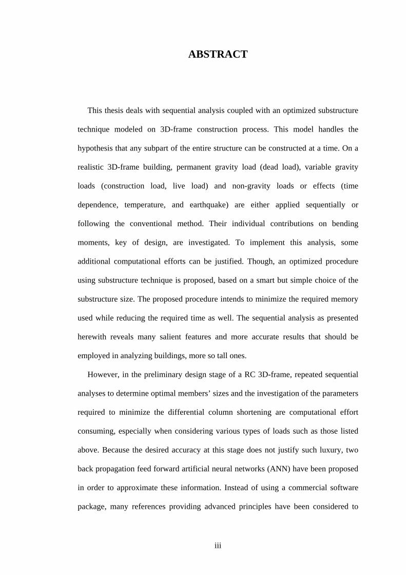
This thesis deals with sequential analysis coupled with an optimized substructure

technique modeled on 3D-frame construction process. This model handles the

hypothesis that any subpart of the entire structure can be constructed at a time. On a

realistic 3D-frame building, permanent gravity load (dead load), variable gravity

loads (construction load, live load) and non-gravity loads or effects (time

dependence, temperature, and earthquake) are either applied sequentially or

following the conventional method. Their individual contributions on bending

moments, key of design, are investigated. To implement this analysis, some

additional computational efforts can be justified. Though, an optimized procedure

using substructure technique is proposed, based on a smart but simple choice of the

substructure size. The proposed procedure intends to minimize the required memory

used while reducing the required time as well. The sequential analysis as presented

herewith reveals many salient features and more accurate results that should be

employed in analyzing buildings, more so tall ones.

However, in the preliminary design stage of a RC 3D-frame, repeated sequential

analyses to determine optimal members’ sizes and the investigation of the parameters

required to minimize the differential column shortening are computational effort

consuming, especially when considering various types of loads such as those listed

above. Because the desired accuracy at this stage does not justify such luxury, two

back propagation feed forward artificial neural networks (ANN) have been proposed

in order to approximate these information. Instead of using a commercial software

package, many references providing advanced principles have been considered to

iv

code a program. The first designed ANN predicts the typical amount of time between

two phases while performing sequential analysis, needed to achieve the minimum

maximorum differential column shortening. The other aims to simulate sequential

analysis results from those of simultaneous analysis. After the training phases, testing

phases have been conducted in order to ensure the generalization ability of these

respective systems. Numerical cases are studied to examine how good these ANN

results match to the finite element method sequential analysis results. Comparison

reveals an acceptable fit; enabling these systems to be safely used in the preliminary

design stage.

Keywords: sequential analysis, substructure technique, computational resources,

artificial neural network, differential column shortening, optimization.

v

ÖZ

Bu tez çalışması 3-boyutlu çerçevelerin yapım aşaması çözümlemesinin, yapısal

bölümleme ile optimize edildiği bir analiz tekniğini içerir. Bu analiz modeli tüm

yapının bir anda yüklenmesi yerine inşa edilme aşamalarına göre analizine dayanır.

Gerçekci 3-boyutlu çerçevelere, kalıcı yerçekim yükü (ölü yük), değişken yerçekim

yükleri (inşaat yükü, haraketli yük) ve diğer yükler ve etkiler (zamana bağlı, sıcaklık

ve deprem) yapım aşamasına ve klasik yönteme göre uygulanmıştır. Bu analizlerin

eğilme momenti ve tasarımdaki rolleri incelenerek karşılaştırılmıştır. Yapım aşaması

analizinin uygulamasında optimizasyonu sağlamak için en uygun yapısal bölünme

boyutu seçilmiştir. Böylece bigisayar çözümü için gerekli hafıza ve zaman minimize

edilmiştir. Bu çalışmada sunulan örneklerle yapım aşaması analizinin önemi, daha

doğru analiz sonuçları için gerekliliği, özellikle yüksek yapılarda öneminin daha da

arttığı ispatlanmıştır.

Ancak 3-boyutlu çerçevelerin ön tasarımı safhasında optimum eleman boyutlarını

ve göreceli kolon kısalmalarını minimize etmek, tekrarlanan yapım aşaması

analizlerinde, yukarıdaki yükler de düşünüldüğünde oldukça güçtür. Bu sebeple bu

aşamada kesin sonuçlara gereksinim duyulmaması sebebi ile yapay sinir ağları

(YSA) ile çok yakın sonuçları verecek iki ağ geliştirilmiştir. Hazır bir paket program

kullanmak yerine, birçok güncel yayın taranarak gelişmiş yöntemleri içerecek şekilde

bir program hazırlanmıştır. Birinci yapay sinir ağı iki yapım aşaması arasında

minimum maksimorum göreceli kolon kısalmasını verecek süreyi hesaplamaktadır.

Diğer yapay sinir ağı ise klasik analiz sonuçlarından, yapım aşaması analiz

sonuçlarını türetmektedir. İlk önce bu iki yapay zeka sisteminin parametreleri

vi

saptanmıştır. Daha sonra bu parametre gurubunun doğru sonuçlar verip vermediği

kontrol edilmiştir. Seçilen örneklerle yapay sinir ağları çözümlerinin sonlu elemanlar

yapım aşaması çözümleriyle örtüştüğü ve ön tasarımda güvenlice kullanılabileceği

ispatlanmıştır.

Anahtar Kelimeler: yapım aşaması analizi, yapısal bölümleme tekniği, işlem

kaynakları, yapay sinir ağları, göreceli kolon kısalması, optimizasyon

vii

DEDICATION

To Paul, Florette, Yvan, Michelle, Clarisse, and Benoit Sepkap

viii

ACKNOWLEDGMENT

I would like to thank Asst. Prof. Dr Giray Özay for his continuous support and

guidance in the preparation of this study. Without his invaluable supervision, all my

efforts could have been short-sighted.

A singular thank goes to Prof. Dr Alagar Rangan for his permanent contributions,

encouragements and support along all my studies. I am also obliged to Asst. Prof. Dr

Alireza Rezaei, Asst. Prof. Dr. Serhan Şensoy, Asst. Prof. Dr Erdinç Soyer, Prof. Dr

Özgür Eren, and Prof. Dr Marifi Güler for their assistance in different ways and at

different stages during my thesis. In addition, numerous friends have always been

assisting me in various ways. I would like to show them gratitude as well.

I owe quite a lot to my family who supported me in many manners all throughout

my studies. I would like to express a deep gratitude to Cedric KOUAMOU W., my

junior brother, for his helpful collaboration.

ix

TABLE OF CONTENTS

ABSTRACT ................................................................................................................ iii

ÖZ ................................................................................................................................. v

DEDICATION ........................................................................................................... vii

ACKNOWLEDGMENT ........................................................................................... viii

LIST OF TABLES ..................................................................................................... xii

LIST OF FIGURES .................................................................................................. xiii

LIST OF SYMBOLS OR ABBREVIATIONS .......................................................... xv

1 INTRODUCTION ..................................................................................................... 1

1.1 General Overview.......................................................................................... 1

1.2 Literature Review .......................................................................................... 2

1.3 Objectives of the Study ................................................................................. 5

1.4 Reasons for Objectives .................................................................................. 6

1.5 Work Done to Achieve Objectives ................................................................ 7

1.6 Achievements ................................................................................................ 8

1.7 Thesis’s Outline ............................................................................................. 9

2 REVIEW OF COMMON LOADS APPLIED ON BUILDINGS ........................... 11

2.1 Dead Load ................................................................................................... 12

2.2 Live Load .................................................................................................... 13

2.3 Construction Loads ..................................................................................... 14

2.4 Temperature Action ..................................................................................... 15

2.5 Time dependent Effect ................................................................................ 15

2.5.1 Compressive Strength ........................................................................... 15

2.5.2 Tensile Strength .................................................................................... 16

x

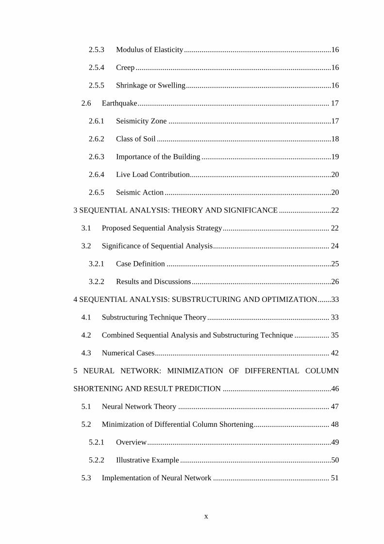
2.5.3 Modulus of Elasticity ............................................................................ 16

2.5.4 Creep ..................................................................................................... 16

2.5.5 Shrinkage or Swelling ........................................................................... 16

2.6 Earthquake ................................................................................................... 17

2.6.1 Seismicity Zone .................................................................................... 17

2.6.2 Class of Soil .......................................................................................... 18

2.6.3 Importance of the Building ................................................................... 19

2.6.4 Live Load Contribution ......................................................................... 20

2.6.5 Seismic Action ...................................................................................... 20

3 SEQUENTIAL ANALYSIS: THEORY AND SIGNIFICANCE ........................... 22

3.1 Proposed Sequential Analysis Strategy ....................................................... 22

3.2 Significance of Sequential Analysis ............................................................ 24

3.2.1 Case Definition ..................................................................................... 25

3.2.2 Results and Discussions ........................................................................ 26

4 SEQUENTIAL ANALYSIS: SUBSTRUCTURING AND OPTIMIZATION ....... 33

4.1 Substructuring Technique Theory ............................................................... 33

4.2 Combined Sequential Analysis and Substructuring Technique .................. 35

4.3 Numerical Cases .......................................................................................... 42

5 NEURAL NETWORK: MINIMIZATION OF DIFFERENTIAL COLUMN

SHORTENING AND RESULT PREDICTION ........................................................ 46

5.1 Neural Network Theory .............................................................................. 47

5.2 Minimization of Differential Column Shortening ....................................... 48

5.2.1 Overview ............................................................................................... 49

5.2.2 Illustrative Example .............................................................................. 50

5.3 Implementation of Neural Network ............................................................ 51

xi

5.3.1 Input Data .............................................................................................. 51

5.3.2 Output Data ........................................................................................... 53

5.3.3 The Training Process ............................................................................ 54

5.3.4 Minimization of Differential Shortening .............................................. 56

5.3.5 Structural Response Prediction ............................................................. 58

6 CONCLUSION AND RECOMMENDATIONS .................................................... 61

6.1 Summary ..................................................................................................... 61

6.2 Conclusion ................................................................................................... 62

6.3 Recommendation for Further Works ........................................................... 63

REFERENCES ........................................................................................................... 65

xii

LIST OF TABLES

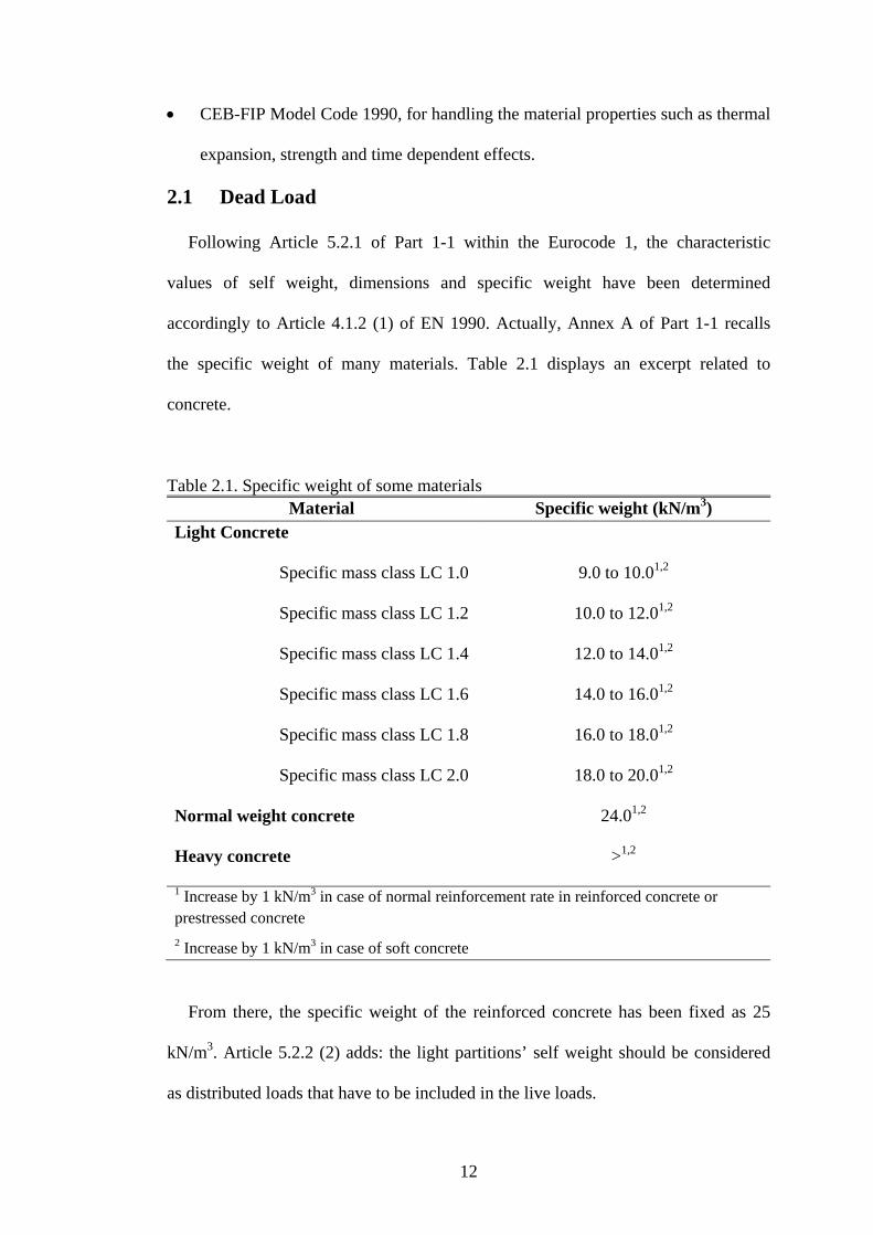
Table 2.1. Specific weight of some materials ............................................................ 12

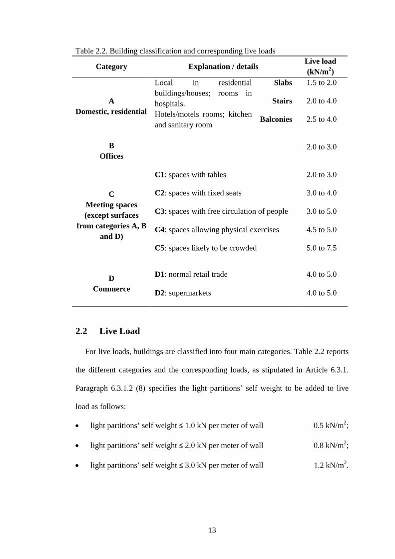
Table 2.2. Building classification and corresponding live loads ............................... 13

Table 2.3. Time dependent cement parameters .......................................................... 15

Table 2.4. Site classification ...................................................................................... 19

Table 2.5. Importance classes of Buildings ............................................................... 19

Table 2.6. Live load participation factor .................................................................... 20

Table 2.7. Values of elastic response spectrum’s parameters .................................... 21

Table 3.1. Dimensions of 3D-frame members in reinforced concrete ........................ 26

Table 3.2. Construction sequence .............................................................................. 26

Table 4.1. Partitioning and regression equation line ................................................... 40

Table 4.2. Optimal substructure size .......................................................................... 40

Table 4.3. Geometric characteristics of study cases .................................................. 43

Table 5.1. Input data for modeling .............................................................................. 52

Table 5.2. Output data for modeling .......................................................................... 54

Table 5.3. Differential shortening Minimization ANN’s training results .................. 57

Table 5.4. Structural response ANN’s training results .............................................. 58

Table 5.5. Illustration and description of the numerical case #2 ............................... 59

Table 5.6. Result report for numerical case #2 .......................................................... 60

Table 5.7. Percentage errors in results for numerical case S2 ................................... 60

xiii

LIST OF FIGURES

Figure 2.1. Seismic zonation map of Cyprus. ............................................................ 18

Figure 2.2. Representation of the elastic response spectrum. .................................... 20

Figure 3.1. Sequential analysis process. ..................................................................... 24

Figure 3.2. Plan configuration of the 15-story building. ............................................ 25

Figure 3.3. Bending moments along the beams of 1st, 5th, 10th and 15th floor. .......... 28

Figure 3.4. Bending moments along the column 3D. (a) Top node. (b) Bottom node.

................................................................................................................ 31

Figure 3.5. Bending moments obtained from earthquake analysis. ........................... 32

Figure 4.1. Representation of 3D-model building. ..................................................... 36

Figure 4.2. Comparison of computation resources. (a) Time. (b) Memory. .............. 38

Figure 4.3. Experiment results in a stepped scatter shape. ........................................ 39

Figure 4.4. Optimization procedure results for the study case. (a) Uncorrected model.

(b) Corrected model. ............................................................................... 41

Figure 4.5. Comparison of computation resources - uncorrected optimization

procedure. (a) Time. (b) Memory. .......................................................... 41

Figure 4.6. Comparison of computation resources - corrected optimization procedure.

(a) Time. (b) Memory. ............................................................................ 42

Figure 4. 7. Comparison of normalized computation resources - three numerical

cases. (a) Time. (b) Memory. ................................................................. 44

Figure 4.8. Main operation steps of the proposed model. .......................................... 45

Figure 5.1. Evolution of maximum differential shortening versus interphase. .......... 51

xiv

Figure 5.2. Typical configuration of ANN for minimization of differential

shortening. .................................................................................................................. 57

Figure 5.3. ANN 1: mapping expected values versus ANN results. .......................... 58

Figure 5.4. Typical configuration of structural response ANN. ................................ 58

Figure 5.5. ANN 2: mapping expected values versus ANN results. .......................... 60

xv

LIST OF SYMBOLS OR ABBREVIATIONS

2D two dimensional

Latin Characters

3D three dimensional

ag design ground acceleration for the return period

A loaded area on a floor

A0 = 10.0 m2

ANN artificial neural network method

CFM correction factor method

CL construction load

CPU central processing unit

DL dead load

𝑒 accuracy of classification expected

𝐸𝑐(28) modulus of elasticity of concrete at 28 days

𝐸𝑝 energy of a neural network system after the presentation of an

arbitrary pattern

𝑒𝑟𝑟𝑜𝑟 error at each output node after the presentation of the last epoch

that corresponds to the end of the training phase

𝑓𝑐𝑘(28) characteristic compressive strength of concrete at 28 days

𝑓𝑐𝑚0 = 10 MPa

𝑓𝑐𝑚(28) mean of compressive strength at 28 days

𝑓𝑒 yielding strength of steel

ℎ number of hidden units

xvi

𝐊 stiffness matrix

LL live load

𝑙𝑥 width of bays in X direction

𝑙𝑦 width of bays in Y direction

𝑙𝑧 height of stories

𝑚 size of stiffness matrix; number of output units

𝑚′ size of stiffness matrix

n story number (n > 2) above the loaded structural elements of

same category; number of input units

N-R normal and rapid hardening

𝑛𝑥 number of bays in X direction

𝑛𝑦 number of bays in Y direction

𝑛𝑧 number of stories in the whole building

𝑝 number of stories constituting the substructure

𝑃 number of training patterns

𝐏 load matrix

𝑝0 critical constant characterizing the number of stories constituting

the substructure

R number of columns at one floor level

𝐑 range of building footprint size

R/C reinforced concrete

RS rapid hardening high strength

S soil factor

𝐒𝑏 resultant boundary force matrix

Se(T) elastic response spectrum

xvii

SL slowly hardening

SM-FEA simultaneous analysis driven along finite element method

SQ-ANN sequential analysis driven along artificial neural network method

SQ-FEA sequential analysis driven along finite element method

SQ-STRU sequential analysis driven along finite element method applied on

the structure as a whole

SQ-SUBS sequential analysis driven along finite element method applied on

the structure regarded as a compilation of many substructures

𝑡 age of concrete; target output value at a given output node;

dummy variable

T vibration period of a linear single-degree-of-freedom system

TB lower limit of the constant spectral acceleration branch

TC upper limit of the constant spectral acceleration branch

TD value defining the beginning of the constant displacement

response range of the spectrum

TD time dependent effect

TL temperature load

𝑡𝑠 age of concrete at the beginning of shrinkage

𝐔 displacement matrix

𝑣∗ positive constant

𝑣𝑚 parameter of a neural network (weight or threshold)

𝑊 energy of a neural network system after the presentation of an

arbitrary pattern with the weight elimination technique

𝑤𝑖𝑗 weight from input unit 𝑖 to hidden unit 𝑗

𝑤𝑗 column of hidden unit 𝑗 into the input-hidden weight matrix

xviii

𝑥 natural input value at a given node

𝑥′ preconditioned input value at a given node

𝑥𝑚𝑎𝑥 maximum natural input value at a given node

𝑥𝑚𝑖𝑛 minimum natural input value at a given node

𝑦 actual output at a given output node; natural output value at a

given node

𝑦′ preconditioned output value at a given node

𝑦𝑚𝑎𝑥 maximum natural output value at a given node

𝑦𝑚𝑖𝑛 minimum natural output value at a given node

𝛼 momentum term

Greek Characters

𝛼𝐴 live load horizontal reduction factor

𝛼𝑛 live load vertical reduction factor

𝛼𝑇 coefficient of thermal expansion

𝛽 scale factor

𝛽0 amplification factor of spectral acceleration for 5% viscous

damping

𝜂 damping correction; gain fraction or step size

𝜆 constant of small positive size

𝜏 counter of the learning process

ѱ0 coefficient as chosen from Annex A.1 of EN 1990

𝑏 boundary

Subscripts

xix

𝑑 down boundary

𝑖 interior

𝑘 dummy variable

𝑢 up boundary

𝑠 dummy variable

𝑡 dummy variable

𝑟 number of substructure

Superscript

1

Chapter 1

INTRODUCTION

1.1 General Overview

Structural engineering calculations aim to choose, for a given structure, the

suitable materials and to define its shapes and dimensions so that it could withstand

safely all the loads applied on. To achieve this purpose, a correct investigation of all

the actual loads and the way they are applied are very critical. Indeed, for any

infrastructure, its erection is a gradual process: one part is constructed after another.

So, loads are progressively generated, and their effects are thereby influenced.

However, as a general observation, structural engineers do not care about this

concern. In fact, they used to consider the structure as a whole, account the possible

loads applied on, and perform any of the available analyses. This happens because

they are not generally aware of this method, and, moreover, very few computer

program packages efficiently incorporate this feature. Therefore, they are

accustomed to practice what is known as simultaneous analysis or straightforward

analysis or conventional analysis (SM-FEA).

As it is presented above, the chronological setting up of different parts

constituting a structure successively generates loads, which consecutively contribute

to the stress development across the structure members. This sequential nature is

accounted by a technique called sequential analysis or segmental analysis or stage

construction analysis (SQ-FEA).

2

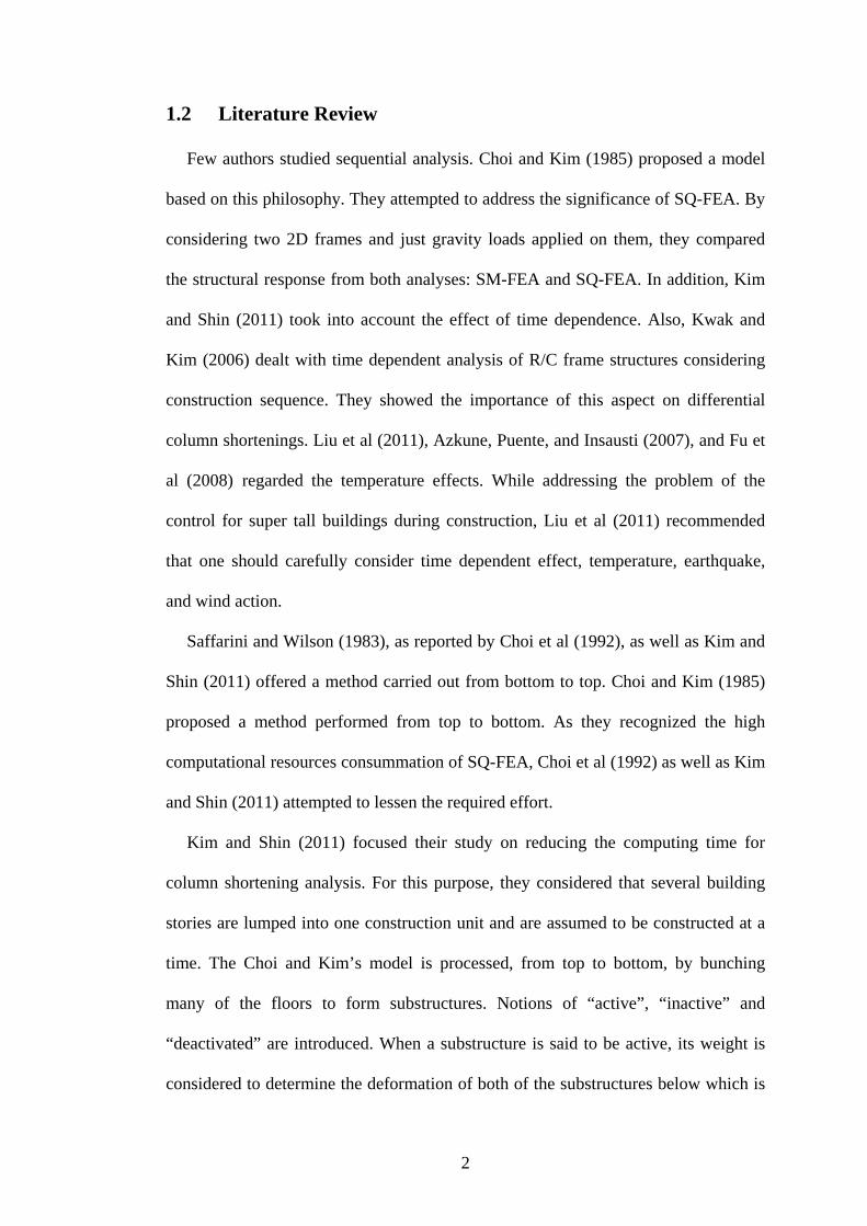
1.2 Literature Review

Few authors studied sequential analysis. Choi and Kim (1985) proposed a model

based on this philosophy. They attempted to address the significance of SQ-FEA. By

considering two 2D frames and just gravity loads applied on them, they compared

the structural response from both analyses: SM-FEA and SQ-FEA. In addition, Kim

and Shin (2011) took into account the effect of time dependence. Also, Kwak and

Kim (2006) dealt with time dependent analysis of R/C frame structures considering

construction sequence. They showed the importance of this aspect on differential

column shortenings. Liu et al (2011), Azkune, Puente, and Insausti (2007), and Fu et

al (2008) regarded the temperature effects. While addressing the problem of the

control for super tall buildings during construction, Liu et al (2011) recommended

that one should carefully consider time dependent effect, temperature, earthquake,

and wind action.

Saffarini and Wilson (1983), as reported by Choi et al (1992), as well as Kim and

Shin (2011) offered a method carried out from bottom to top. Choi and Kim (1985)

proposed a method performed from top to bottom. As they recognized the high

computational resources consummation of SQ-FEA, Choi et al (1992) as well as Kim

and Shin (2011) attempted to lessen the required effort.

Kim and Shin (2011) focused their study on reducing the computing time for

column shortening analysis. For this purpose, they considered that several building

stories are lumped into one construction unit and are assumed to be constructed at a

time. The Choi and Kim’s model is processed, from top to bottom, by bunching

many of the floors to form substructures. Notions of “active”, “inactive” and

“deactivated” are introduced. When a substructure is said to be active, its weight is

considered to determine the deformation of both of the substructures below which is

3

said to be inactive, and the active substructure itself. So, the part of the structure

above called deactivated, has been deformed in the previous stage of the analysis.

Although the aforementioned studies provided sound results, they did not give

enough attention to some important aspects. Choi and Kim’s model neglected the

effects of the deformation that occurred in the inactive substructure due to its weight,

in evaluating the behavior of the active substructure. The reverse way of this process,

for example makes it difficult for any adaptation in case of change in the number of

stories. Also, the substructuring model that Choi and Kim (1985) as well as Kim and

Shin (2011) proposed assumes the entire substructure to be constructed at a time, a

fact that reduces the accuracy of the analysis.

Surprisingly, along their models, none of these studies states, clearly, how to size

the substructure or the lumps. They aimed to trim down separately either the size of

equations or the needed time, but never both in the same process. Among those who

address the contribution of elementary loads, none considered many of them together

in order to show the influence of one load to another’s effect; and none accounted the

respective effect of construction load, live load and earthquake.

Anyway, all of them and other authors agreed that the differences between the two

analyses are due to the: (1) differential column shortening (Choi and Kim, 1985); (2)

sequential application of dead load (Choi and Kim, 1985; Fu et al, 2008; Ozay and

Njomo, 2012a), and temperature actions (Fu et al, 2008; Ozay and Njomo, 2012a;

Azkune, Puente, and Insausti, 2007); (3) aging, creep, and shrinkage of the concrete

(Kwak and Kim, 2006; Fu et al, 2008; Ozay and Njomo, 2012a); and (4)

consideration of the coming and going of construction loads (Fu et al, 2008; Ozay

and Njomo, 2012a).

4

Differential column shortening may affect non structural elements (Fintel, Ghosh,

and Iyengar, 1986), aesthetic appearance, and the normal use of edifices. To decrease

its effects, Fintel, Ghosh and Iyengar (1986) developed a compensation method.

Herein, for the same goal, a minimization model has been proposed. Given a

structure destined to some use, made in a definite-characteristic material and located

in a particular environment, the structural response depends on the timing of the

construction sequence. Thus, the amount of the differential shortening is function of

the interphase, i.e. the typical duration between two consecutive stages.

On the other hand, considering all actions and trying to reduce the effect of

differential column shortening while performing SQ-FEA calls for much more

computational effort than SM-FEA since it requires many intermediate computations

in addition to the final stage analysis that “corresponds” to the simultaneous analysis.

But regarding the accuracy and the features carried by this strategy, this excess

demand is justified, though it needs to be lowered. Some research works tried to

accomplish this purpose by getting SQ-FEA’s results from those of SM-FEA.

Choi et al (1992) proposed the so called correction factor method (CFM) based on

regression analysis. They claimed to well approximate SQ-FEA’s results considering

only dead loads on 2D frames. Gupta and Sharma (2001) reported that Khan (1997)

developed a neural network which simulates results of SQ-FEA from those of one

stage analysis. They accounted that the neural net did not take into account the time

dependent effect. These models are not realistic since they do not depict the actual

situation of edifices: buildings are neither bi-dimensional nor protected against time

dependent effects which contribute among others to the differential movement, but

they are, in addition to dead loads, submitted under many other actions.

5

Even though, the seriousness of these studies has been recognized among the

scientific community, the gap as presented above is still present. Moreover, the

regression analysis used by Choi et al may suffer from constraints such as the linear

or curvilinear relationship of the data with heteroscedatic error (Walczak and Cerpa,

1999). Khan (1997) tried to overcome this limitation with a multilayer feedforward

neural network. He took profit to the fact that this system is a universal function

approximator that can interpolate between vectors (Gupta and Sharma, 2011;

Walczak and Cerpa, 1999; Belic I, 2012, pp. 3-22; Leondes, 1998; Iliadis and Jayne

C, 2011; Fausett L, 1994; Haykin, 2005).

Nevertheless, it is capital to provide a tool to reduce the computational effort

needed to obtain near accurate results as well as to determine the sequence’s

interphase with the intention to be able to make good decision in the earlier stage of

preliminary study (Gupta and Sharma, 2011); since it is the project phase that is the

most influential in the total cost (Haroglu et al, 2009; Ballal and Sher, 2003). In the

present thesis, the soft computing tool artificial neural network is held to take down

the computational effort and the differential column shortening on R/C 3D frame.

Various types of loads are considered. These include dead loads, time dependent

effects, temperature actions, construction forces and live load. Seismic loads are not

considered here since they induce similar structural response whether considering

sequential analysis or simultaneous analysis (Ozay and Njomo, 2012a).

1.3 Objectives of the Study

Different goals drove this study. In general, all tried to promote the sequential

analysis while reducing the computational effort it requires.

6

a. The first goal accounted various loads sequentially applied and investigated

their actual respective contribution. By this way, it expected to exhibit the

significance of the SQ-FEA.

b. The second goal was to reduce the computational resources required to

perform sequential analysis.

c. The third goal determined the optimal duration between two phases, yielding

to a minimum differential column shortening.

d. The fourth goal predicted the sequential analysis results from those of

simultaneous ones.

1.4 Reasons for Objectives

The convergence of these goals contributes to bridge from the SM-FEA to the

SQ-FEA with less effort.

a. Isolating the individual contribution of a particular load points out the

difference of sequential analysis versus simultaneous analysis. It may also be

helpful to decide whether it is enough to consider simultaneous analysis for

some loading cases or not. Anyway, the significance of SQ-FEA is

underscored.

b. Sequential analysis consists in performing analyses at various stages and

requires storing information for the next stage. As a result, it is needed a lot of

CPU memory and a large amount of computational time. Nowadays, the

demand of efficient algorithm is competitively growing. Although many

computers are much performing than ever, the increasing complexity of

buildings may make them unable to solve some problems if the algorithm is

not carefully studied.

7

c. Differential column shortening has a negative effect at various points of a

project: it affect the aesthetical aspect, the normal functionality of the

infrastructure, and even the non structural elements. So, it is a great advantage

to economically and environment-friendly reduce this facet by just fine-tuning

the construction timing.

d. At earlier stage of a project study, namely preliminary design phase where the

optimal structural systems are looked for, it is a profligacy to complete the

repeated SQ-FEAs with results of 100% accuracy. Instead, a workaround may

consist in carrying out the SM-FEA, and approximate from their results those

for SQ-FEA.

1.5 Work Done to Achieve Objectives

The different goals targeted herein have been overcome by finite element analysis

followed by either statistical model or artificial neural network tool.

a. A realistic R/C 3D frame representing a middle-rise building, an everyday’s

situation, has been submitted under various loading cases. The structural

responses from both simultaneous and sequential analysis have been peeled

off and the isolated effect of each loading case from one analysis has been

compared with its corresponding version from the other analysis.

b. To reduce the computational resources needed, the sequential analysis has

been coupled with the substructure technique. Finite element analysis has been

applied on several numerical cases, and a statistical model has been drawn to

optimize the obtained merger (SQ-SUBS).

c. Many buildings ranging throughout the practical interval have been analyzed

with the finite element method through the sequential scheme. For each one,

the result was the optimal duration yielding to minimal differential column

8

shortening. A neural network has been trained to simulate the relationship

between the building characteristics and the optimal duration.

d. As in the previous point, the same buildings, analyzed with SQ-FEA, provided

vectors to develop an ANN. It aims to approximate the SQ-FEA results from

those of SM-FEA in order to get SQ-ANN.

1.6 Achievements

In general, all the objectives contribute to emphasize on the importance of the

sequential analysis while proposing efficient algorithms or practical tools to reduce

the computational effort it requires, with the intention to contribute to the

implementation of proficient software packages.

a. By investigating the contributions of different loading cases, it appeared that

some of them are kept almost the same whether SQ-FEA or SM-FEA. On the

other side, some happened to be very sensitive to SQ-FEA. This information

has been revealed to be important when these latter loads are predominant in a

project or may be useful to decide whether to conduct SQ-FEA or not. Overall,

the significance of SQ-FEA over the SM-FEA has been highlighted since the

final combined structural response has been too divergent.

b. The statistical model designed from the results of many building analyses

ended to an optimized merger: a substructure sizing method has been

developed with the intention to minimize the CPU memory and the time

needed to SQ-SUBS computations. The implication of the substructure

technique will not influence the analysis accuracy.

c. Given any R/C 3D frame determined by obvious properties like the number of

stories or the ambient temperature change, an ANN has be trained to predict

9

which construction duration between two stories would minimize the maximal

differential column shortening.

d. A simple method based on ANN tool, intending to approximately deduct SQ-

FEA results from those of SM-FEA has been trained; this happens to be very

helpful for example during the phase of preliminary design when the accuracy

provided by the repeated and resource consuming SQ-FEA is a luxury. The

SQ-ANN’s results showed that ANNs are good tools to settle this fastidious

problem.

1.7 Thesis’s Outline

This thesis is made of five other chapters. All of them convey to achieve the

points mentioned above. In the following chapter, all the different loads involved in

this study have been assessed: dead load, live load, time dependent effects,

temperature action, and earthquake. Their values have been adopted along the

respective code prescriptions.

Then, in the third chapter, the sequential analysis theory is stated. The issue of

column differential shortening is clearly studied here. Furthermore, the respective

contribution of each loading type has been evaluated in the SQ-FEA versus SM-

FEA. The result has been to emphasize the significance of the sequential method.

Chapter 4 recalled the substructure technique, and coupled this technique with the

SQ-FEA. The aim of this part (SQ-SUBS) has been to shorten the computational

resources required for SQ-STRU. Numerical cases have been considered to illustrate

the results.

After that, the theory about the soft computing neural network has been reported

in the fifth chapter. Many references have been considered in order to facilitate its

implementation. Plus, this chapter dealt with the acute problematic of approaching

10

the sequential results in the design stage. Two artificial neural networks have been

developed to estimate the step duration yielding to minimum maximorum differential

shortening on the one hand, and, on the other, to approximate SQ-FEA’s results from

those of simultaneous one.

Finally, Chapter 6 ends the present thesis. It has been devoted to the general

summary of the current work. Recommendations and further works have been also

proposed.

11

Chapter 2

REVIEW OF COMMON LOADS APPLIED ON

BUILDINGS

Many criteria can be used to classify loads applied on buildings. One can choose

to distinguish mechanical loads (dead load, live load, construction load, wind action

and earthquake) from non- mechanical ones (time dependent effect and temperature).

Some may opt to differentiate gravity loads (dead load, live load, and construction

load) versus non-gravity ones (time dependent effect, temperature, wind action and

earthquake); or others, to separate lateral loads (wind action and earthquake) from

non-lateral ones (dead load, live load, construction load, time dependent effect, and

temperature). This last classification system has been the concern of the present

work. Herein, all the non-lateral loads have been considered, but the wind action has

been neglected compared to the earthquake effect.

Because of the location of the numerical cases and their availability in software

packages, the current study has been based on:

• Eurocode 1 : « Bases de Calculs et Actions sur les Structures et Documents

d’Application Nationale, » for estimations of dead load, live load, construction

load, and temperature action;

• Eurocode 8 : « Conception et dimensionnement des structures pour leur

résistance aux séismes et documents d’application nationale », plus “A review of

the seismic hazard zonation in national building codes in the context of

Eurocode 8” for all computations related to earthquake, and;

12

• CEB-FIP Model Code 1990, for handling the material properties such as thermal

expansion, strength and time dependent effects.

2.1 Dead Load

Following Article 5.2.1 of Part 1-1 within the Eurocode 1, the characteristic

values of self weight, dimensions and specific weight have been determined

accordingly to Article 4.1.2 (1) of EN 1990. Actually, Annex A of Part 1-1 recalls

the specific weight of many materials. Table 2.1 displays an excerpt related to

concrete.

Table 2.1. Specific weight of some materials Material Specific weight (kN/m3)

Light Concrete

Specific mass class LC 1.0 9.0 to 10.01,2

Specific mass class LC 1.2 10.0 to 12.01,2

Specific mass class LC 1.4 12.0 to 14.01,2

Specific mass class LC 1.6 14.0 to 16.01,2

Specific mass class LC 1.8 16.0 to 18.01,2

Specific mass class LC 2.0 18.0 to 20.01,2

Normal weight concrete 24.01,2

Heavy concrete >1,2

1 Increase by 1 kN/m3 in case of normal reinforcement rate in reinforced concrete or prestressed concrete 2 Increase by 1 kN/m3 in case of soft concrete

From there, the specific weight of the reinforced concrete has been fixed as 25

kN/m3. Article 5.2.2 (2) adds: the light partitions’ self weight should be considered

as distributed loads that have to be included in the live loads.

13

Table 2.2. Building classification and corresponding live loads

Category Explanation / details Live load (kN/m2)

Local in residential buildings/houses; rooms in hospitals. Hotels/motels rooms; kitchen and sanitary room

Slabs 1.5 to 2.0

A Domestic, residential

Stairs 2.0 to 4.0

Balconies 2.5 to 4.0

B Offices

2.0 to 3.0

C Meeting spaces (except surfaces

from categories A, B and D)

C1: spaces with tables 2.0 to 3.0

C2: spaces with fixed seats 3.0 to 4.0

C3: spaces with free circulation of people 3.0 to 5.0

C4: spaces allowing physical exercises 4.5 to 5.0

C5: spaces likely to be crowded 5.0 to 7.5

D Commerce

D1: normal retail trade 4.0 to 5.0

D2: supermarkets 4.0 to 5.0

2.2 Live Load

For live loads, buildings are classified into four main categories. Table 2.2 reports

the different categories and the corresponding loads, as stipulated in Article 6.3.1.

Paragraph 6.3.1.2 (8) specifies the light partitions’ self weight to be added to live

load as follows:

• light partitions’ self weight ≤ 1.0 kN per meter of wall 0.5 kN/m2;

• light partitions’ self weight ≤ 2.0 kN per meter of wall 0.8 kN/m2;

• light partitions’ self weight ≤ 3.0 kN per meter of wall 1.2 kN/m2.

14

Paragraph 6.3.1.2 (9) concerns the heavy partitions. Paragraph 6.3.1.2 (10) and

Paragraph 6.3.1.2 (11) deals with the horizontal and vertical reduction factor. The

horizontal reduction factor 𝛼𝐴 is determined as follows:

𝛼𝐴 = min( 57

ѱ0 + 𝐴0𝐴

; 1.0) (2.1)

with 𝛼𝐴 ≥ 0.6 for categories C and D, and where

ѱ0 is the coefficient as chosen from Annex A.1 of EN 1990. ѱ0 = 0.7 for the

categories discussed above;

𝐴0 = 10.0 m2;

𝐴 is the loaded area.

For the vertical reduction factor 𝛼𝑛, it is obtained by:

𝛼𝑛 = 2+(𝑛−2)ѱ0𝑛

(2.2)

where 𝑛 is the story number (𝑛 > 2) above the loaded structural elements of same

category.

Herein, these recommendations have been simplified and an overall value for live

load has been adopted. Also, the roof has been considered with the same use as the

other floor. Anyway, these simplifications do not reduce the seriousness of the

targeted goal, but just alleviate the calculation process for a better comprehension.

2.3 Construction Loads

Part 2-6 gives an interest on action during work execution. It includes amongst

other loads, the construction loads which are defined as loads other than

environmental and climatic in nature, and which have to be considered in the design

during the construction process. Article 4.8.1 (2) stipulates that it is suitable to these

actions to be evaluated accordingly to the project’s specifications.

15

2.4 Temperature Action

The temperature action matter is provided by Part 2-5. Article 5.1.3 (3) authorizes

to suppose a uniform temperature distribution for common buildings where the

computations are required. It adds that national maps showing isotherms of

temperature from Stevenson screen can be used.

Article 2.1.8.3 of CEB-FIP Model Code 1990 proposes to take the coefficient of

thermal expansion as 𝛼𝑇 = 10 × 10−6 𝐾−1 for structural analysis. It must be noted

that the temperature dependence of materials has not been accounted in the scope of

this study.

2.5 Time dependent Effect

The main source discussing about time dependent effects is CEB-FIP Model Code

1990. This code provides formulas to predict the characteristics of R/C along the

time. Compressive strength, tensile strength, modulus of elasticity, creep, and

shrinkage have been all concerned herein.

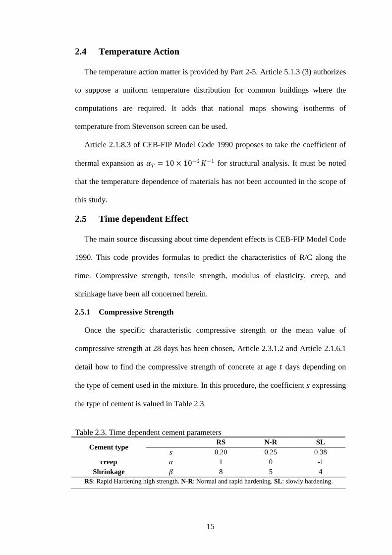
2.5.1 Compressive Strength

Once the specific characteristic compressive strength or the mean value of

compressive strength at 28 days has been chosen, Article 2.3.1.2 and Article 2.1.6.1

detail how to find the compressive strength of concrete at age 𝑡 days depending on

the type of cement used in the mixture. In this procedure, the coefficient 𝑠 expressing

the type of cement is valued in Table 2.3.

Table 2.3. Time dependent cement parameters

Cement type RS N-R SL 𝑠 0.20 0.25 0.38

creep 𝛼 1 0 -1 Shrinkage 𝛽 8 5 4

RS: Rapid Hardening high strength. N-R: Normal and rapid hardening. SL: slowly hardening.

16

2.5.2 Tensile Strength

The tensile strength is firmly dependent on the specific characteristic compressive

strength according to Article 2.1.3.3.1.

2.5.3 Modulus of Elasticity

Article 2.1.4.2 gives the value of the modulus of elasticity at 28 days from the

mean of compressive strength at 𝑡 = 28 𝑑𝑎𝑦𝑠. It states that

𝐸𝑐(28) = 21500 [𝑓𝑐𝑚(28)𝑓𝑐𝑚0

]13 with 𝑓𝑐𝑚0 = 10 𝑀𝑃𝑎. The modulus of elasticity of

concrete at any date may be predicted from that at 28 days and the type of cement, as

described in Article 2.1.6.3; thus it is also dependent on the mean of compressive

strength at 28 days.

2.5.4 Creep

Expressed in terms of creep compliance or creep function, the creep is treated in

Article 2.1.6.4.3. It is related to the creep coefficient, the modulus of elasticity at 28

days, and the modulus of elasticity at the loading age which is also dependent of that

at 28 days as seen in section 2.5.3 of the present thesis. The creep coefficient is a

product of two quantities: the notional creep coefficient and a time dependent

coefficient describing the creep development after loading. These two quantities vary

in respect of the relative humidity of the ambient environment, the member’s cross

section dimensions, and the age of the concrete at the loading. In addition, the former

changes with the variation of the mean value of compressive strength at 28 days, as

well.

2.5.5 Shrinkage or Swelling

The total shrinkage/swelling strains at 𝑡 days are concerned in Article 2.1.6.4.4. It

may be obtained from two parameters. The first is the notional shrinkage coefficient

which may be calculated from the relative humidity of the ambient environment, the

17

mean of compressive strength at 28 days, and a cement dependent shrinkage

coefficient from Table 2.3. On the other hand, the second parameter is a time

dependent coefficient describing the shrinkage/swelling development. It is a function

of the age of concrete at the beginning of shrinkage/swelling and the cross sectional

geometry of the structural member.

In conclusion, the non-lateral forces as described above are mainly dependent on:

• the specific weight of the constituting material (which is constant for R/C);

• the member’s cross section dimensions;

• the member’s lengths;

• the whole structure’s geometry;

• the use of the edifice;

• the external temperature;

• the type of cement used in concrete mixture;

• the mean value of compressive strength at 28 days;

• the relative humidity of the ambient environment;

• the age of the concrete at the loading;

• the age of the concrete at the beginning of the shrinkage/swelling.

These few parameters can be said to be determinant in the assessment of the non-

lateral loads applied on an R/C 3D frame structure, and, thus, in the prediction of its

structural response with respect to these loads.

2.6 Earthquake

2.6.1 Seismicity Zone

Analyses to withstand against earthquake are fundamentally dependent on seismic

hazard. Locations are divided into different seismic hazard levels within each

country. In particular, Prof C. Chrysostomou prepared a personal communication

18

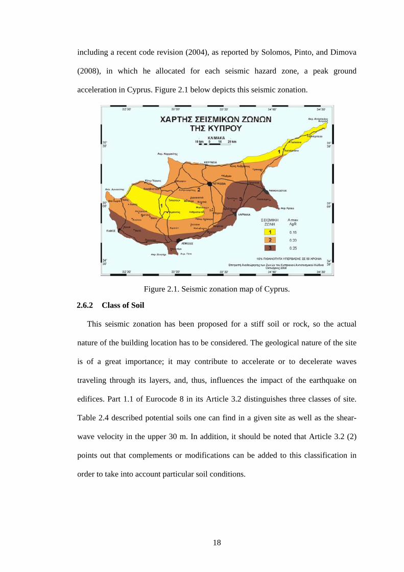
including a recent code revision (2004), as reported by Solomos, Pinto, and Dimova

(2008), in which he allocated for each seismic hazard zone, a peak ground

acceleration in Cyprus. Figure 2.1 below depicts this seismic zonation.

Figure 2.1. Seismic zonation map of Cyprus.

2.6.2 Class of Soil

This seismic zonation has been proposed for a stiff soil or rock, so the actual

nature of the building location has to be considered. The geological nature of the site

is of a great importance; it may contribute to accelerate or to decelerate waves

traveling through its layers, and, thus, influences the impact of the earthquake on

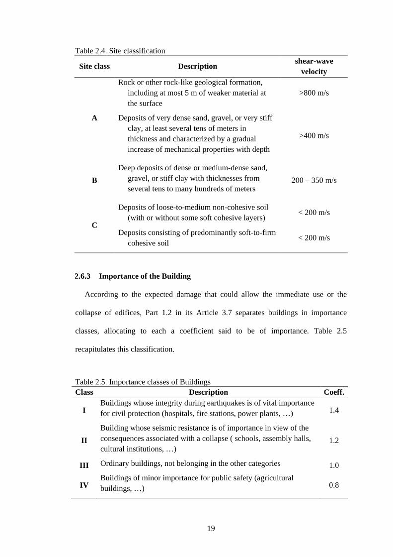
edifices. Part 1.1 of Eurocode 8 in its Article 3.2 distinguishes three classes of site.

Table 2.4 described potential soils one can find in a given site as well as the shear-

wave velocity in the upper 30 m. In addition, it should be noted that Article 3.2 (2)

points out that complements or modifications can be added to this classification in

order to take into account particular soil conditions.

19

Table 2.4. Site classification

Site class Description shear-wave velocity

A

Rock or other rock-like geological formation, including at most 5 m of weaker material at the surface

>800 m/s

Deposits of very dense sand, gravel, or very stiff clay, at least several tens of meters in thickness and characterized by a gradual increase of mechanical properties with depth

>400 m/s

B Deep deposits of dense or medium-dense sand,

gravel, or stiff clay with thicknesses from several tens to many hundreds of meters

200 – 350 m/s

C

Deposits of loose-to-medium non-cohesive soil (with or without some soft cohesive layers)

< 200 m/s

Deposits consisting of predominantly soft-to-firm cohesive soil

< 200 m/s

2.6.3 Importance of the Building

According to the expected damage that could allow the immediate use or the

collapse of edifices, Part 1.2 in its Article 3.7 separates buildings in importance

classes, allocating to each a coefficient said to be of importance. Table 2.5

recapitulates this classification.

Table 2.5. Importance classes of Buildings Class Description Coeff.

I Buildings whose integrity during earthquakes is of vital importance for civil protection (hospitals, fire stations, power plants, …) 1.4

II Building whose seismic resistance is of importance in view of the consequences associated with a collapse ( schools, assembly halls, cultural institutions, …)

1.2

III Ordinary buildings, not belonging in the other categories 1.0

IV Buildings of minor importance for public safety (agricultural buildings, …) 0.8

20

2.6.4 Live Load Contribution

To consider the probability that the live load may not fully be present at the

instant an earthquake occurs, coefficients fixing the contribution of the live load are

available. Also, they account the partial participation to the structure’s motion of

non-firmly fixed masses. It is given below in Table 2.6 for the common buildings as

studied in Section 2.1 of the present thesis, as specified in Article 3.6 of Part 1.2.

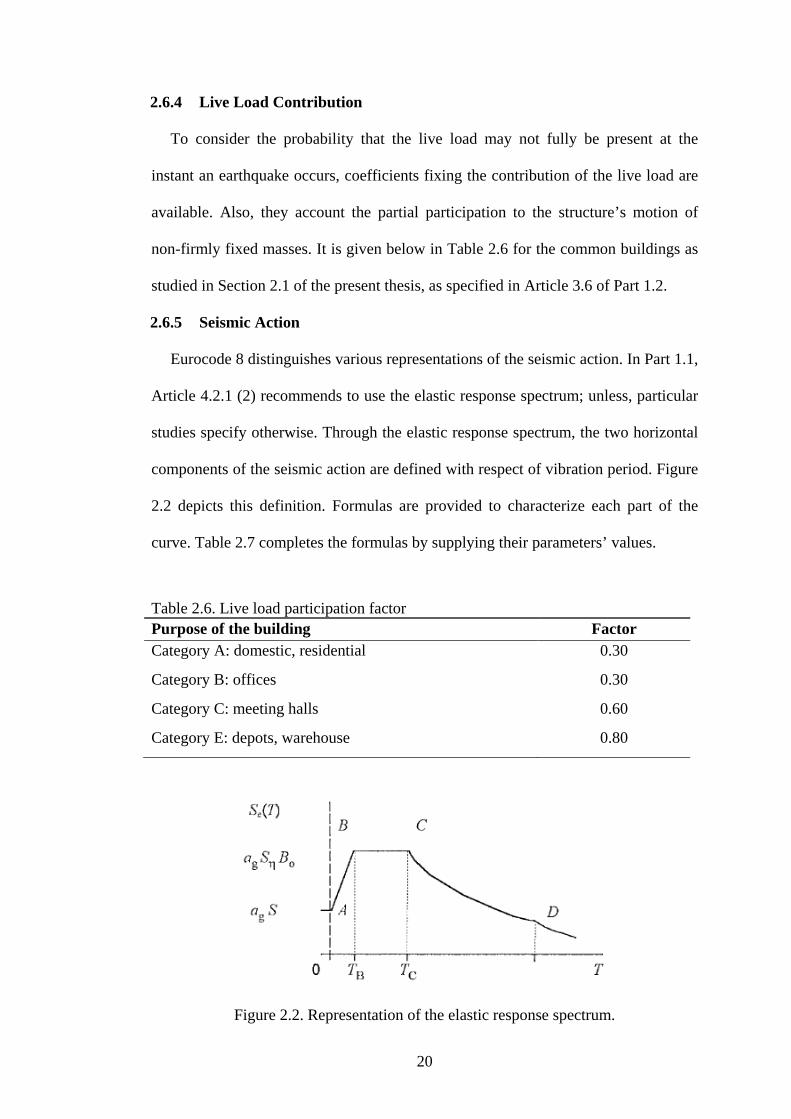
2.6.5 Seismic Action

Eurocode 8 distinguishes various representations of the seismic action. In Part 1.1,

Article 4.2.1 (2) recommends to use the elastic response spectrum; unless, particular

studies specify otherwise. Through the elastic response spectrum, the two horizontal

components of the seismic action are defined with respect of vibration period. Figure

2.2 depicts this definition. Formulas are provided to characterize each part of the

curve. Table 2.7 completes the formulas by supplying their parameters’ values.

Table 2.6. Live load participation factor Purpose of the building Factor Category A: domestic, residential 0.30

Category B: offices 0.30

Category C: meeting halls 0.60

Category E: depots, warehouse 0.80

Figure 2.2. Representation of the elastic response spectrum.

21

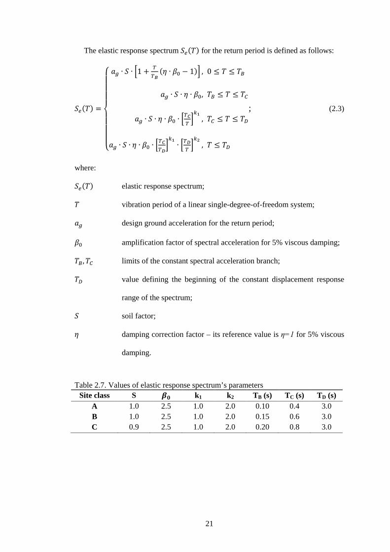
The elastic response spectrum 𝑆𝑒(𝑇) for the return period is defined as follows:

𝑆𝑒(𝑇) =

⎩⎪⎪⎪⎨

⎪⎪⎪⎧ 𝑎𝑔 ∙ 𝑆 ∙ �1 + 𝑇

𝑇𝐵(𝜂 ∙ 𝛽0 − 1)� , 0 ≤ 𝑇 ≤ 𝑇𝐵

𝑎𝑔 ∙ 𝑆 ∙ 𝜂 ∙ 𝛽0, 𝑇𝐵 ≤ 𝑇 ≤ 𝑇𝐶

𝑎𝑔 ∙ 𝑆 ∙ 𝜂 ∙ 𝛽0 ∙ �𝑇𝐶𝑇�𝑘1

, 𝑇𝐶 ≤ 𝑇 ≤ 𝑇𝐷

𝑎𝑔 ∙ 𝑆 ∙ 𝜂 ∙ 𝛽0 ∙ �𝑇𝐶𝑇𝐷�𝑘1∙ �𝑇𝐷

𝑇�𝑘2

, 𝑇 ≤ 𝑇𝐷

�; (2.3)

where:

𝑆𝑒(𝑇) elastic response spectrum;

𝑇 vibration period of a linear single-degree-of-freedom system;

𝑎𝑔 design ground acceleration for the return period;

𝛽0 amplification factor of spectral acceleration for 5% viscous damping;

𝑇𝐵,𝑇𝐶 limits of the constant spectral acceleration branch;

𝑇𝐷 value defining the beginning of the constant displacement response

range of the spectrum;

𝑆 soil factor;

𝜂 damping correction factor – its reference value is η=1 for 5% viscous

damping.

Table 2.7. Values of elastic response spectrum’s parameters Site class S 𝜷𝟎 k1 k2 TB (s) TC (s) TD (s)

A 1.0 2.5 1.0 2.0 0.10 0.4 3.0 B 1.0 2.5 1.0 2.0 0.15 0.6 3.0 C 0.9 2.5 1.0 2.0 0.20 0.8 3.0

22

Chapter 3

SEQUENTIAL ANALYSIS: THEORY AND

SIGNIFICANCE

Choi and Kim (1985) described a strategy to perform SQ-FEA. However, it is

maculated of some limitations affecting the result accuracy. Plus, since the authors

regarded only dead load, the strategy does not point how to include the other loading

types. The following paragraphs propose a sequential analysis strategy modeled on

the construction process; it accounts various loads: dead load, live load, construction

load, time dependent effect, temperature, and earthquake. The proposed model leads

to more realistic results.

3.1 Proposed Sequential Analysis Strategy

Sequential analysis of a given building consists of successive analyses at different

dates along the construction process. The typical schedule considered herein is to set

each story erection as a phase. At the beginning, the first story is erected and put over

formwork. The new cast structure is left for a definite period, termed as interphase,

while getting hard. During this elapsing period, it undergoes temperature stresses and

time dependent effects. An analysis is conducted in order to determine the structural

response at the end of this stage. It shows that this part of the structure has performed

deformations and presents internal forces across its members.

After that, the story is stricken and the second floor is constructed over shores

supported by the existing slab. Instead of keeping the idealized length of column in

this new floor, the top is leveled at the designed position. From this moment and

23

during the interphase, the first floor supports its own dead load, the construction

loads from the second floor, temperature action and time dependent effects; and the

second floor is submitted under temperature stresses and time dependent effects.

Once more, a second analysis is completed considering the deformed shape of the

existing structure as reference. This new analysis regards the first story as weightless

since its weight has been already considered in the first analysis, but it takes into

account the temperature action and the time dependent effect occurred during the last

interphase. The analysis reveals a new structural response which is cumulated to the

previous one.

At the end of the second period, the third floor comes; and the part of the

structure, constituted by the first and the second stories serves altogether as the first

one, while the third as the second of the preceding phase. Here, the construction

loads formerly applied on the first slab is removed. Operations are repeated till the

last floor which is not subjected to any construction load, but to the all remaining

load types. After an appropriate analysis, like finite element method for example, has

been performed and structural response summed up, the live load is applied along

with temperature action and time dependent effect considering the deformed

geometry as reference.

In this thesis, for non-lateral loads, even if the deformed shape has been accounted

for the elastic stiffness, displacements and deformations have been assumed to be

relatively small so that the equilibrium equations could be stated using the idealized

shape and the geometric stiffness matrix could be neglected. However, this aspect

has been considered when the displacements became large, for example in the case

of earthquake, as prescribed by Przemieniecki (1968).

24

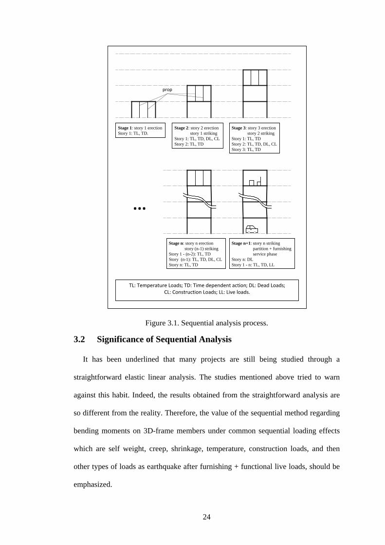
Figure 3.1. Sequential analysis process.

3.2 Significance of Sequential Analysis

It has been underlined that many projects are still being studied through a

straightforward elastic linear analysis. The studies mentioned above tried to warn

against this habit. Indeed, the results obtained from the straightforward analysis are

so different from the reality. Therefore, the value of the sequential method regarding

bending moments on 3D-frame members under common sequential loading effects

which are self weight, creep, shrinkage, temperature, construction loads, and then

other types of loads as earthquake after furnishing + functional live loads, should be

emphasized.

Stage 1: story 1 erectionStory 1: TL, TD.

Stage 2: story 2 erection story 1 strikingStory 1: TL, TD, DL, CLStory 2: TL, TD

Stage 3: story 3 erection story 2 strikingStory 1: TL, TDStory 2: TL, TD, DL, CLStory 3: TL, TD

Stage n: story n erection story (n-1) strikingStory 1 - (n-2): TL, TDStory (n-1): TL, TD, DL, CLStory n: TL, TD

Stage n+1: story n striking partition + furnishing service phaseStory n: DLStory 1 - n: TL, TD, LL

...

TL: Temperature Loads; TD: Time dependent action; DL: Dead Loads;CL: Construction Loads; LL: Live loads.

prop

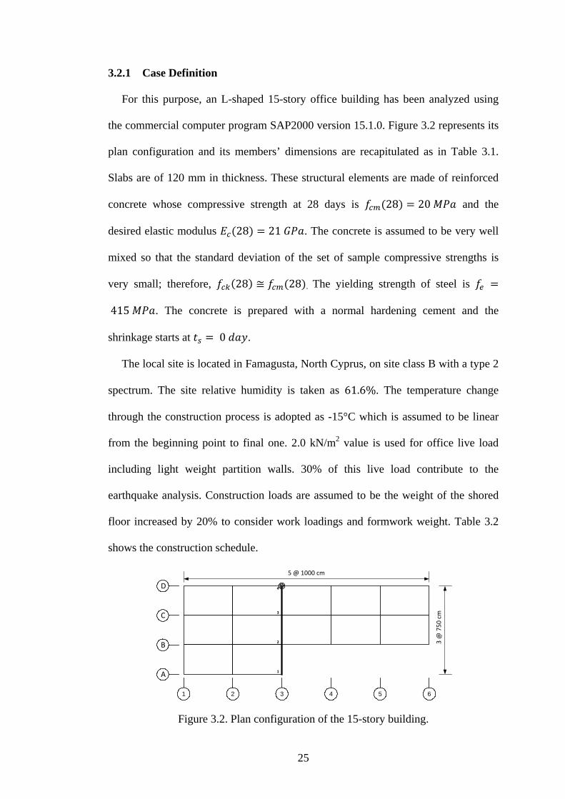
25

3.2.1 Case Definition

For this purpose, an L-shaped 15-story office building has been analyzed using

the commercial computer program SAP2000 version 15.1.0. Figure 3.2 represents its

plan configuration and its members’ dimensions are recapitulated as in Table 3.1.

Slabs are of 120 mm in thickness. These structural elements are made of reinforced

concrete whose compressive strength at 28 days is 𝑓𝑐𝑚(28) = 20 𝑀𝑃𝑎 and the

desired elastic modulus 𝐸𝑐(28) = 21 𝐺𝑃𝑎. The concrete is assumed to be very well

mixed so that the standard deviation of the set of sample compressive strengths is

very small; therefore, 𝑓𝑐𝑘(28) ≅ 𝑓𝑐𝑚(28). The yielding strength of steel is 𝑓𝑒 =

415 𝑀𝑃𝑎. The concrete is prepared with a normal hardening cement and the

shrinkage starts at 𝑡𝑠 = 0 𝑑𝑎𝑦.

The local site is located in Famagusta, North Cyprus, on site class B with a type 2

spectrum. The site relative humidity is taken as 61.6%. The temperature change

through the construction process is adopted as -15°C which is assumed to be linear

from the beginning point to final one. 2.0 kN/m2 value is used for office live load

including light weight partition walls. 30% of this live load contribute to the

earthquake analysis. Construction loads are assumed to be the weight of the shored

floor increased by 20% to consider work loadings and formwork weight. Table 3.2

shows the construction schedule.

Figure 3.2. Plan configuration of the 15-story building.

5 @ 1000 cm

3 @

750

cm

2

3

4

1

1 2 3 4 5 6

A

C

B

D

26

Table 3.1. Dimensions of 3D-frame members in reinforced concrete Floor Member Width × Depth (cm) Cross area of concrete (cm2) 1-15 Beam 25 × 60 1500

10-15 Column 30 × 60 1800 7-10 40 × 60 2400 1-6 60 × 60 3600

Table 3.2. Construction sequence Stage Duration (in days) Added Structure Operations

1 10 Story 1 2 10 Story 2 Striking story 1 3 10 Story 3 Striking story 2 4 10 Story 4 Striking story 3 5 10 Story 5 Striking story 4 6 10 Story 6 Striking story 5 7 10 Story 7 Striking story 6 8 10 Story 8 Striking story 7 9 10 Story 9 Striking story 8 10 10 Story 10 Striking story 9 11 10 Story 11 Striking story 10 12 10 Story 12 Striking story 11 13 10 Story 13 Striking story 12 14 10 Story 14 Striking story 13 15 10 Story 15 Striking story 14

16 10 Striking story 15;

partition and furnishing; service phase

3.2.2 Results and Discussions

Once SQ-FEA and SM-FEA have been performed, attention has been given on

the frame 3 in Figure 3.2. Moments have been regarded along the beams of the 1st,

the 5th, the 10th and the 15th story, as well as both but separately, at the top and

bottom of each column of the chain 3D encircled in the figure. These quantities are

compared in terms of differences given as percentage of the corresponding bending

moments obtained from straightforward analysis, taken as reference.

27

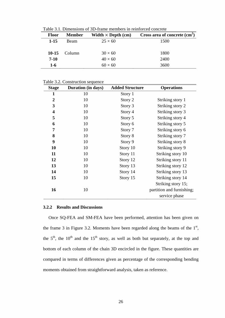
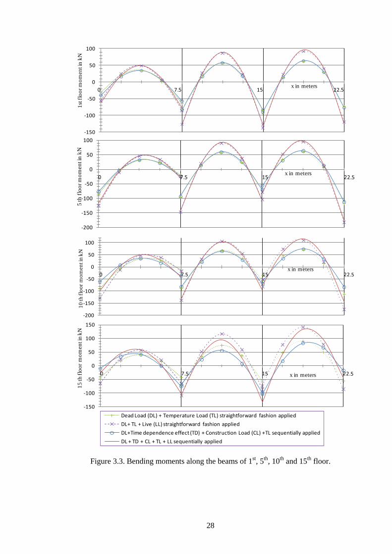
Figure 3.3 presents the bending moments along the selected beams. The following

inferences can be made from the figure:

• The two analyses yield to much bunchy moments in the lower floors than in the

upper ones where a difference of 62% has been observed. This confirms the fact,

reported by Choi and Kim (1985) and Kwak and Kim (2006), that the sequential

analysis is more important for tall buildings.

• Sequential analysis tends to reduce the difference of moments from one side to

another of the intermediate columns. At the second support of the 15th story

beam, SQ-FEA shows a moment difference of 7% from one side to another and

SM-FEA a difference of 41%. By reducing this difference, the column behaves

safer and does not require so much reinforcement. Also, the reinforcement

applied for superior layer in one side of the beam can be extended to the other

side without major losses for practical convenience.

• The span with irregularity (the first one) exhibits more difference than the spans

with regularities. This result may also be extended for the global case of a whole

building: irregular edifices are more sensitive to the difference SQ-FEA versus

SM-FEA than regular ones.

• The live loads, applied at a time for both analyses, reduce the divergence between

them. For example, the difference changes from 80% to 62% at the first support

of the upper beam.

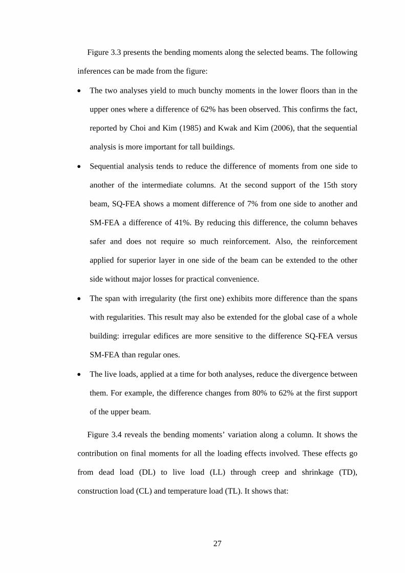
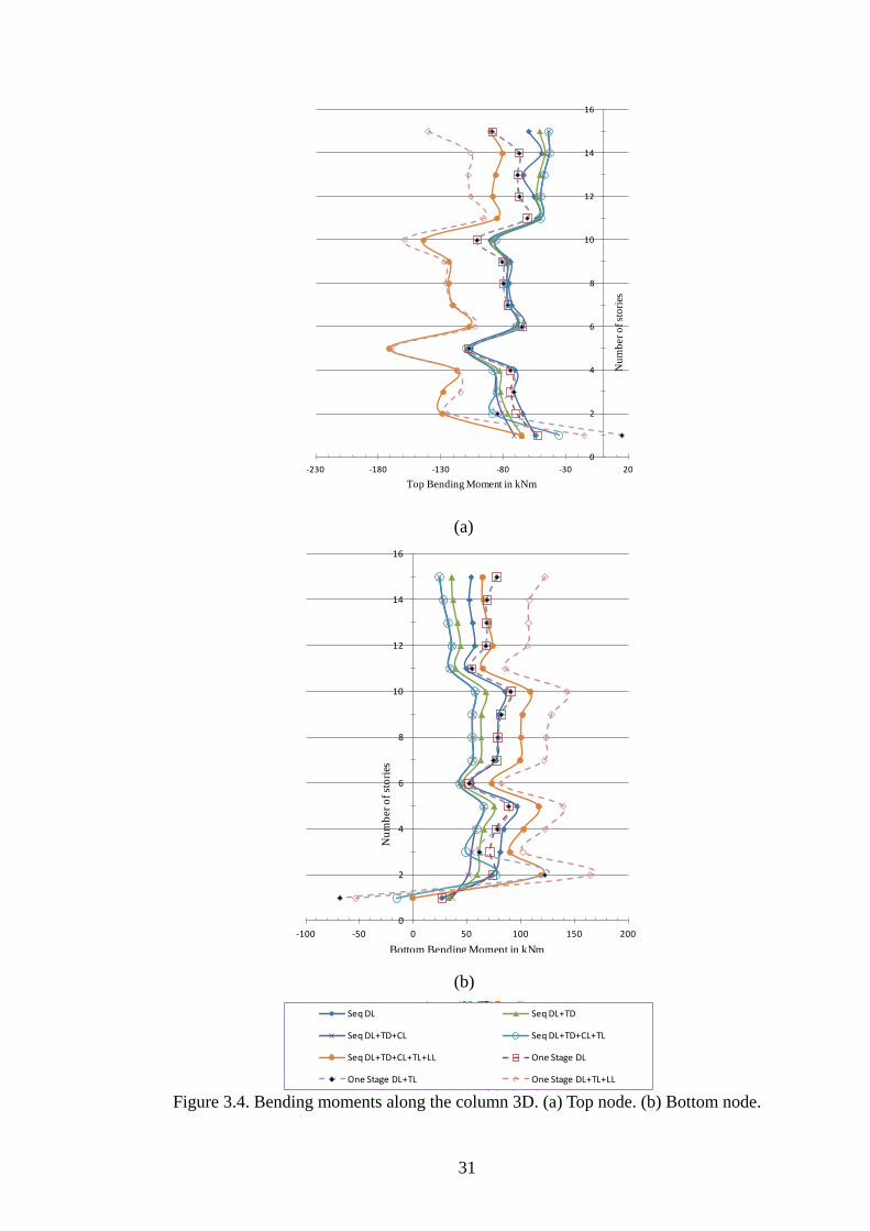
Figure 3.4 reveals the bending moments’ variation along a column. It shows the

contribution on final moments for all the loading effects involved. These effects go

from dead load (DL) to live load (LL) through creep and shrinkage (TD),

construction load (CL) and temperature load (TL). It shows that:

28

Figure 3.3. Bending moments along the beams of 1st, 5th, 10th and 15th floor.

-150

-100

-50

0

50

100

1st f

loor

mom

ent i

n kN

x in meters

-200

-150

-100

-50

0

50

100

5 th

floo

r mom

ent i

n kN

x in meters

-200

-150

-100

-50

0

50

100

10 th

floo

r mom

ent i

n kN

x in meters

-150

-100

-50

0

50

100

150

15 th

floo

r mom

ent i

n kN

x in meters

Dead Load (DL) + Temperature Load (TL) straightforward fashion appliedDL+ TL + Live (LL) straightforward fashion appliedDL+Time dependence effect (TD) + Construction Load (CL) +TL sequentially appliedDL + TD + CL + TL + LL sequentially applied

29

i) Top Moment

• The time dependent effect causes a change varying from -20% to +20%.

• The consideration of construction loads is significant since it generates a moment

variation from -14% to 10%.

• These two previous effects act more significantly at the extremities of the whole

structure.

• The temperature does not have a major effect except in the lower floors where it

may reduce the response of the structure by 50% for sequential analysis and

completely inverse the sign of the moment for straightforward analysis from -

65.36 kNm to +14.49 kNm. Temperature applied at a time causes more structural

response than considering it applied sequentially;

• The shape of the final moment curve is dictated by the curve when temperature is

considered.

• The live load tends to reduce the difference between the two analyses. A change

from 50.7% to 35.6% can be noticed.

• Above floor 5, the straightforward analysis yields to redundant internal forces, up

to 35.6%.

• But, below floor 5, it yields to unsafe results varying from -1.2% to -76.3%

difference.

ii) Bottom Moment

• The time dependent moment’s curve seems to keep a progressive variation with

+23.5% change at floor 1, -18.7% at floor 2 to - 33.6% at floor 15.

30

• Similarly, the construction load moment curve keeps the same progressive

variation along the structure height with +9.5% at floor 1, -13.8% at floor 2 to -

32.6% at floor 15.

• The temperature load is insignificant in the upper stories but causes +49.3%

change in the 2nd story and inverse the sign of the moment in the 1st floor, from

+35.62 kNm to -15.43 kNm for sequential analysis. Also here, sequential

temperature stresses the structure less than temperature applied at the time.

• The shape of the final curve is once more dictated by the curve when considering

temperature.

• The sequential analysis yields to more economical results for up to 98.7 %.

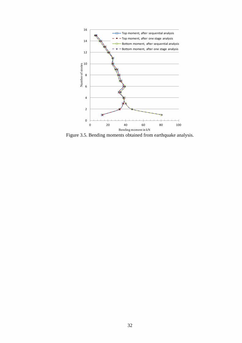
The same structure is also analyzed under the earthquake with two initial shapes:

first, considering the un-deformed shape of the total structure; and second, after the

deformation happened due to previous loads. The mass centers of these two initial

shapes form the vector (0.7 mm, 0.1 mm, -7.6 mm) whose length is 7.7 mm. The

moments obtained from these analyses are not significantly divergent. This mass

center translation and the overall deformation of the structure after sequential

analysis are insignificant regarding the effect of the earthquake. Figure 3.5 explains

the resulting moments.

31

(a)

(b)

Figure 3.4. Bending moments along the column 3D. (a) Top node. (b) Bottom node.

0

2

4

6

8

10

12

14

16

-230 -180 -130 -80 -30 20

Num

ber o

f sto

ries

Top Bending Moment in kNm

0

2

4

6

8

10

12

14

16

-100 -50 0 50 100 150 200

Num

ber o

f sto

ries

Bottom Bending Moment in kNm

8

10

Seq DL Seq DL+TD

Seq DL+TD+CL Seq DL+TD+CL+TL

Seq DL+TD+CL+TL+LL One Stage DL

One Stage DL+TL One Stage DL+TL+LL

32

Figure 3.5. Bending moments obtained from earthquake analysis.

0

2

4

6

8

10

12

14

16

0 20 40 60 80 100

Num

ber o

f sto

ries

Bending moment in kN

Top moment, after sequential analysis

Top moment, after one stage analysis

Bottom moment, after sequential analysis

Bottom moment, after one stage analysis

33

Chapter 4

SEQUENTIAL ANALYSIS: SUBSTRUCTURING AND

OPTIMIZATION

Although Choi and Kim (1985) as well as Kim and Shin (2011) ingeniously

attempted to merged SQ-FEA with substructuring technique with the intention to

lessen the effort required to conduct the lengthy SQ-FEA driven along finite element

method applied on the structure as a whole (SQ-STRU), they failed by losing the full

accuracy. In addition, as already stated in Chapter 1, they treated separately the

memory and the time. Hereinafter, it is proposed an SQ-FEA coupled with optimized

substructuring technique (SQ-SUBS) that encompasses time and memory and

provides a sizing method of the optimal substructure.

4.1 Substructuring Technique Theory

It is well known that dealing with large matrices requires much of the computer

memory and operational time. Substructuring aspires to reduce the size of the

involved matrices by dividing the entire structure into smaller substructures.

Przemieniecki (1963) presented a matrix structural analysis of substructures and

extensively described it in his book (Przemieniecki, 1968, pp 231-263). Later, He,

Zhou and Hou (2008), and Leung (1979) used and recommended this technique to

simplify the analysis of mega-structures.

Any given structure can be divided into 𝑛 substructures separated by the

boundaries constituting the set of nodes named boundary nodes. The remaining

34

nodes of each substructure are called interior nodes. So, for the rth substructure, the

well known equation

𝐊(𝑟)𝐔(𝑟) = 𝐏(𝑟) (4.1)

can be written as

�𝐊𝑏𝑏

(𝑟) 𝐊𝑏𝑖(𝑟)

𝐊𝑖𝑏(𝑟) 𝐊𝑖𝑖

(𝑟)� �𝐔𝑏

(𝑟)

𝐔𝑖(𝑟)� = �

𝐏𝑏(𝑟)

𝐏𝑖(𝑟)�. (4.2)

Here, 𝐊, 𝐔 and 𝐏 stand for stiffness, displacement and load while the subscripts 𝑏

and 𝑖 stand for boundary and interior, respectively. The boundary matrix of one

substructure is obtained from

𝐊𝑏(𝑟) = 𝐊𝑏𝑏

(𝑟) − 𝐊𝑏𝑖(𝑟)(𝐊𝑖𝑖

(𝑟))−1𝐊𝑖𝑏(𝑟). (4.3)

All these matrices are combined into a large one forming the stiffness boundary

matrix 𝐊𝑏 for the entire subdivided structure. After relaxation, the resultant boundary

force matrix is

𝐒𝑏 = 𝐏𝑏 − ∑ 𝐊𝑏𝑖(𝑟)(𝐊𝑖𝑖

(𝑟))−1𝐏𝑖(𝑟)𝑛

𝑟=1 (4.4)

where 𝐏𝑏 is the boundary force matrix corresponding to 𝐊𝑏. The boundary

displacements are determined from

𝐔𝑏 = (𝐊𝑏)−1𝐒𝑏. (4.5)

Now, to calculate the interior displacements the boundary displacement matrix is

divided into n substructure-boundary-displacement matrices, as

𝐔𝑖(𝑟) = (𝐊𝑖𝑖

(𝑟))−1𝐏𝑖(𝑟) − (𝐊𝑖𝑖

(𝑟))−1𝐊𝑖𝑏(𝑟)𝐔𝑏

(𝑟). (4.6)

Having obtained all node displacements, the rest of the analysis can follow within

each substructure as the conventional displacement method. It can readily be

observed that the sizes of matrices involved in this calculation are less than the sizes

of the corresponding matrices involved in the entire-structure analysis (SQ-STRU).

35

Especially, the entire structure stiffness matrix is reduced provided that the interior

nodes exist.

However, in the majority of cases there is no interior node in a floor. Since the

efficiency of the substructuring technique is dependent on these interior nodes, it is

necessary to take many floors as one substructure at a given stage of analysis. One

should note that the lumped stories are not considered as constructed at the same

time but regrouped only for the displacement determination. At this instant, only the

penultimate floor weight is accounted as dead load self supported since the last floor

is still shored up by formworks. Also, if the typical substructure consists of very few

stories, the boundary matrix 𝐊𝑏’s size will not so much differ from the whole

stiffness matrix. On the other hand, if the substructure is too large, interior-to-interior

submatrices 𝐊𝑖𝑖, which are mainly subjected to inversion, will also be too large.

These two extreme cases will make the substructuring less efficient. The next section

proposes a method which optimizes the substructuring. In other words, it will answer

the question ‘how to size the substructure to minimize the computation resources,

say, time and memory’.

4.2 Combined Sequential Analysis and Substructuring Technique

Consider a 3D-frame building under its dead load and construction load as

represented in Figure 4.1 given below. At any arbitrary construction stage, only the

penultimate floor’s weight is accounted for the analysis of the already-constructed

part of the building which is analyzed by using substructuring technique. Therefore,

Eq. (4.2) can be rewritten as

�𝐊𝑑𝑑

(𝑟) 𝐊𝑑𝑖(𝑟) 𝐊𝑑𝑢

(𝑟)

𝐊𝑖𝑑(𝑟) 𝐊𝑖𝑖

(𝑟) 𝐊𝑖𝑢(𝑟)

𝐊𝑢𝑑(𝑟) 𝐊𝑢𝑖

(𝑟) 𝐊𝑢𝑢(𝑟)

� �𝐔𝑑

(𝑟)

𝐔𝑖(𝑟)

𝐔𝑢(𝑟)

� = �𝟎𝐏𝑖

(𝑟)

𝟎�; (4.7)

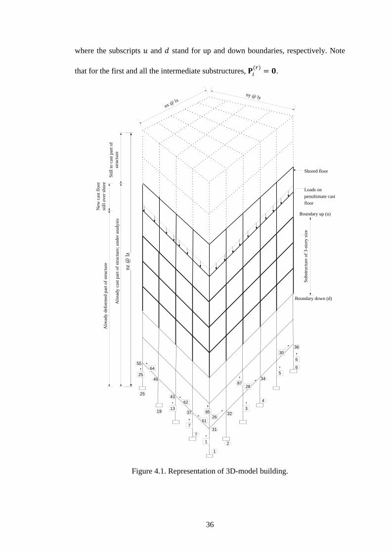
36

where the subscripts 𝑢 and 𝑑 stand for up and down boundaries, respectively. Note

that for the first and all the intermediate substructures, 𝐏𝑖(𝑟) = 𝟎.

Figure 4.1. Representation of 3D-model building.

1

Alre

ady

defo

rmed

par

t of s

truct

ure

Subs

truct

ure

of 3

-sto

ry si

ze

4

6

7

19

25

31

32

34

36

37

43

49

55

1

3

5

6

7

13

25

26

28

30

61

62

64

85

87

Boundary down (d)

Boundary up (u)

Still

to c

ast p

art o

f st

ruct

ure

Loads on penultimate cast floor

Alre

ady

cast

par

t of s

truct

ure;

und

er a

naly

sis

nz @

lz

2

Shored floor

New

cas

t flo

or

still

ove

r sho

renx @ lx

ny @ ly

37

In this model, 𝐊𝑠𝑡(𝑟) (𝑠, 𝑡 = 𝑑,𝑢) is an 𝑚 × 𝑚 square matrix; the size 𝑚 = 6𝑅

where R is the number of columns at one floor level. For the actual case of a regular

rectangular building footprint, 𝑅 = (𝑛𝑥 + 1)(𝑛𝑦 + 1), where 𝑛𝑥 and 𝑛𝑦 are the

number of bays in X and Y directions, respectively. The rest of 𝐊𝑠𝑡(𝑟), where at least

one of 𝑠 or 𝑡 is 𝑖, are either a 𝑚′ × 𝑚 / 𝑚 × 𝑚′ rectangular or a 𝑚′ × 𝑚′ square

matrix. The maximum size is 𝑚′ = 𝑚(𝑝 − 1) = 6(𝑝 − 1)𝑅 with 𝑝 denoting the

number of stories constituting the substructure. Thus the size of each submatrix

depends on 𝑅, the number of columns at any given floor level.

Remembering that in such a computation process the operation complexity

depends on the size of the matrix, it is noticeable that the optimal size of

substructure, 𝑝, will also depend on R. Considering only gravity loads during the

construction, and a schedule in which each floor is stricken before the construction of

the next one, two procedures have been developed in the computer algebra system

Wolfram Mathematica version 7.0 running with a laptop working under Windows 7

Home basic, with a CPU Intel Core i5-480M, 2.66 GHz and a 4 GB RAM.

Procedure A considers SQ-FEA of buildings without substructuring (SQ-STRU)

while procedure B considers substructuring (SQ-SUBS). Each of these procedures

takes the stiffness matrix of each element in its current shape, as input. Then, after

having constituted the convenient load matrix, it assembles all these stiffness

matrices in the relevant form and yields the displacements.

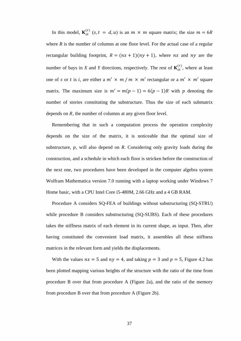
With the values 𝑛𝑥 = 5 and 𝑛𝑦 = 4, and taking 𝑝 = 3 and 𝑝 = 5, Figure 4.2 has

been plotted mapping various heights of the structure with the ratio of the time from

procedure B over that from procedure A (Figure 2a), and the ratio of the memory

from procedure B over that from procedure A (Figure 2b).

38

(a)

(b)

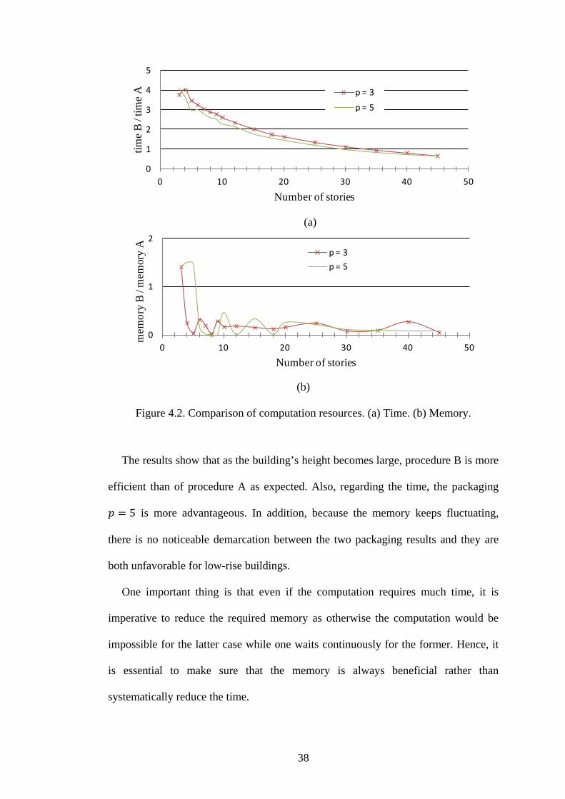
Figure 4.2. Comparison of computation resources. (a) Time. (b) Memory.

The results show that as the building’s height becomes large, procedure B is more

efficient than of procedure A as expected. Also, regarding the time, the packaging

𝑝 = 5 is more advantageous. In addition, because the memory keeps fluctuating,

there is no noticeable demarcation between the two packaging results and they are

both unfavorable for low-rise buildings.

One important thing is that even if the computation requires much time, it is

imperative to reduce the required memory as otherwise the computation would be

impossible for the latter case while one waits continuously for the former. Hence, it

is essential to make sure that the memory is always beneficial rather than

systematically reduce the time.

0

1

2

3

4

5

0 10 20 30 40 50

time

B /

time

A

Number of stories

p = 3

p = 5

0

1

2

0 10 20 30 40 50

mem

ory

B /

mem

ory

A

Number of stories

p = 3p = 5

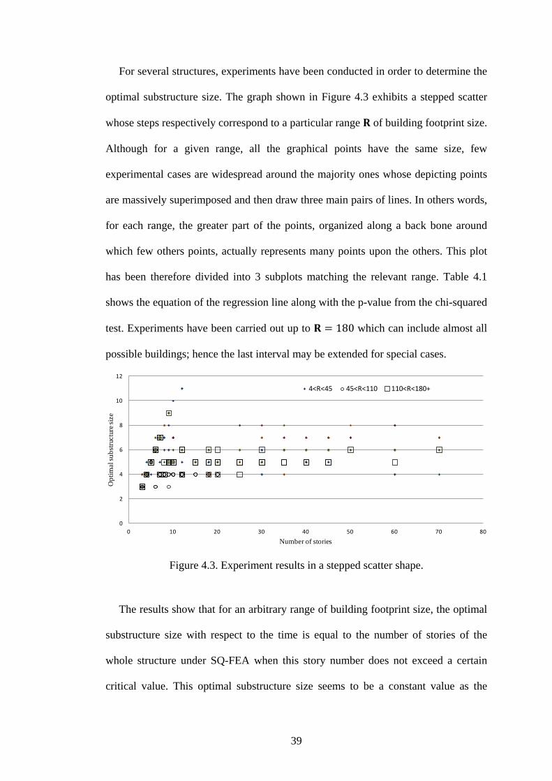
39

For several structures, experiments have been conducted in order to determine the

optimal substructure size. The graph shown in Figure 4.3 exhibits a stepped scatter

whose steps respectively correspond to a particular range 𝐑 of building footprint size.

Although for a given range, all the graphical points have the same size, few

experimental cases are widespread around the majority ones whose depicting points

are massively superimposed and then draw three main pairs of lines. In others words,

for each range, the greater part of the points, organized along a back bone around

which few others points, actually represents many points upon the others. This plot

has been therefore divided into 3 subplots matching the relevant range. Table 4.1

shows the equation of the regression line along with the p-value from the chi-squared

test. Experiments have been carried out up to 𝐑 = 180 which can include almost all

possible buildings; hence the last interval may be extended for special cases.

Figure 4.3. Experiment results in a stepped scatter shape.

The results show that for an arbitrary range of building footprint size, the optimal

substructure size with respect to the time is equal to the number of stories of the

whole structure under SQ-FEA when this story number does not exceed a certain

critical value. This optimal substructure size seems to be a constant value as the

0

2

4

6

8

10

12

0 10 20 30 40 50 60 70 80

Opt

imal

subs

truct

ure s

ize

Number of stories

4<R<45 45<R<110 110<R<180+

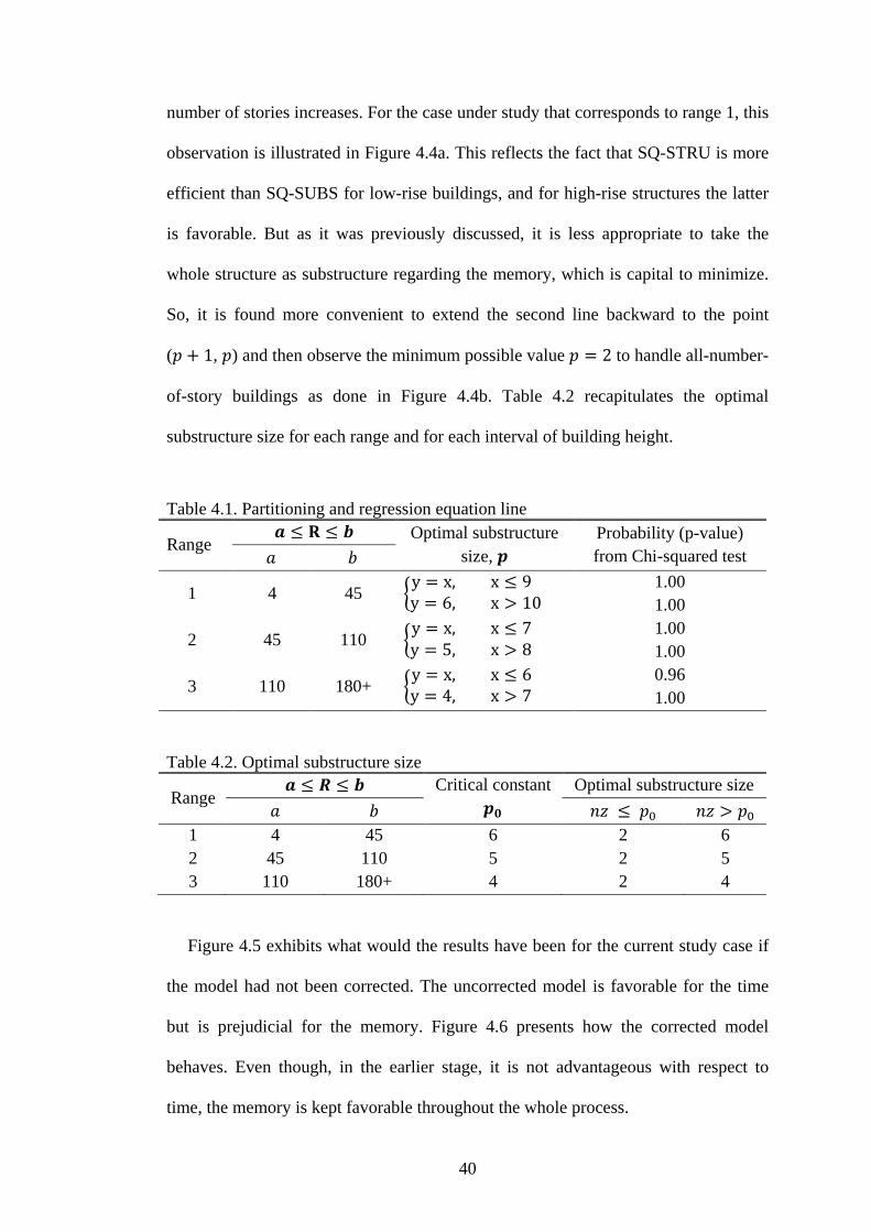
40

number of stories increases. For the case under study that corresponds to range 1, this

observation is illustrated in Figure 4.4a. This reflects the fact that SQ-STRU is more

efficient than SQ-SUBS for low-rise buildings, and for high-rise structures the latter

is favorable. But as it was previously discussed, it is less appropriate to take the

whole structure as substructure regarding the memory, which is capital to minimize.

So, it is found more convenient to extend the second line backward to the point

(𝑝 + 1, 𝑝) and then observe the minimum possible value 𝑝 = 2 to handle all-number-

of-story buildings as done in Figure 4.4b. Table 4.2 recapitulates the optimal

substructure size for each range and for each interval of building height.

Table 4.1. Partitioning and regression equation line

Range 𝒂 ≤ 𝐑 ≤ 𝒃 Optimal substructure

size, 𝒑 Probability (p-value) from Chi-squared test 𝑎 𝑏

1 4 45 �y = x, x ≤ 9y = 6, x > 10

� 1.00 1.00

2 45 110 �y = x, x ≤ 7y = 5, x > 8

� 1.00 1.00

3 110 180+ �y = x, x ≤ 6y = 4, x > 7

� 0.96 1.00

Table 4.2. Optimal substructure size

Range 𝒂 ≤ 𝑹 ≤ 𝒃 Critical constant

𝒑𝟎 Optimal substructure size

𝑎 𝑏 𝑛𝑧 ≤ 𝑝0 𝑛𝑧 > 𝑝0 1 4 45 6 2 6 2 45 110 5 2 5 3 110 180+ 4 2 4

Figure 4.5 exhibits what would the results have been for the current study case if

the model had not been corrected. The uncorrected model is favorable for the time

but is prejudicial for the memory. Figure 4.6 presents how the corrected model

behaves. Even though, in the earlier stage, it is not advantageous with respect to

time, the memory is kept favorable throughout the whole process.

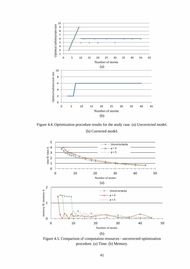
41

(a)

(b)

Figure 4.4. Optimization procedure results for the study case. (a) Uncorrected model.

(b) Corrected model.

(a)

(b)

Figure 4.5. Comparison of computation resources - uncorrected optimization procedure. (a) Time. (b) Memory.

23456789

10

0 5 10 15 20 25 30 35 40 45 50Opt

imal

subs

truct

ure s

ize

Number of stories

0

2

4

6

8

10

0 5 10 15 20 25 30 35 40 45

Opt

imal

subs

truct

ure

size

Number of stories

012345

0 10 20 30 40 50

time B

/ tim

e A

Number of stories

Uncorrected pp = 3p = 5

0

1

2

0 10 20 30 40 50

mem

ory

B / m

emor

y A

Number of stories

Uncorrected pp = 3p = 5

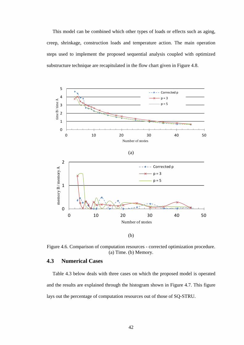
42

This model can be combined which other types of loads or effects such as aging,

creep, shrinkage, construction loads and temperature action. The main operation

steps used to implement the proposed sequential analysis coupled with optimized

substructure technique are recapitulated in the flow chart given in Figure 4.8.

(a)

(b)

Figure 4.6. Comparison of computation resources - corrected optimization procedure. (a) Time. (b) Memory.

4.3 Numerical Cases

Table 4.3 below deals with three cases on which the proposed model is operated

and the results are explained through the histogram shown in Figure 4.7. This figure

lays out the percentage of computation resources out of those of SQ-STRU.

0

1

2

3

4

5

0 10 20 30 40 50

time B

/ tim

e A

Number of stories

Corrected p

p = 3

p = 5

0

1

2

0 10 20 30 40 50

mem

ory

B / m

emor

y A

Number of stories

Corrected p

p = 3

p = 5

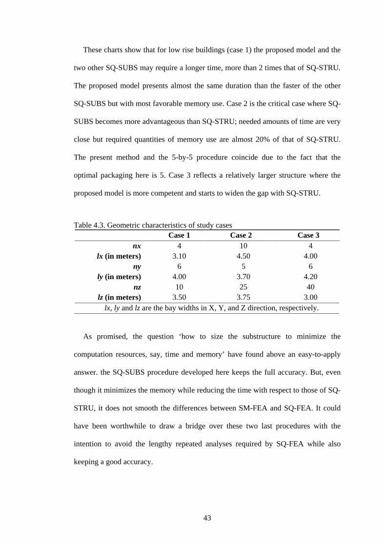
43

These charts show that for low rise buildings (case 1) the proposed model and the

two other SQ-SUBS may require a longer time, more than 2 times that of SQ-STRU.

The proposed model presents almost the same duration than the faster of the other

SQ-SUBS but with most favorable memory use. Case 2 is the critical case where SQ-

SUBS becomes more advantageous than SQ-STRU; needed amounts of time are very

close but required quantities of memory use are almost 20% of that of SQ-STRU.

The present method and the 5-by-5 procedure coincide due to the fact that the

optimal packaging here is 5. Case 3 reflects a relatively larger structure where the

proposed model is more competent and starts to widen the gap with SQ-STRU.

Table 4.3. Geometric characteristics of study cases Case 1 Case 2 Case 3

nx 4 10 4 lx (in meters) 3.10 4.50 4.00

ny 6 5 6 ly (in meters) 4.00 3.70 4.20

nz 10 25 40 lz (in meters) 3.50 3.75 3.00

lx, ly and lz are the bay widths in X, Y, and Z direction, respectively.

As promised, the question ‘how to size the substructure to minimize the

computation resources, say, time and memory’ have found above an easy-to-apply

answer. the SQ-SUBS procedure developed here keeps the full accuracy. But, even

though it minimizes the memory while reducing the time with respect to those of SQ-

STRU, it does not smooth the differences between SM-FEA and SQ-FEA. It could

have been worthwhile to draw a bridge over these two last procedures with the

intention to avoid the lengthy repeated analyses required by SQ-FEA while also

keeping a good accuracy.

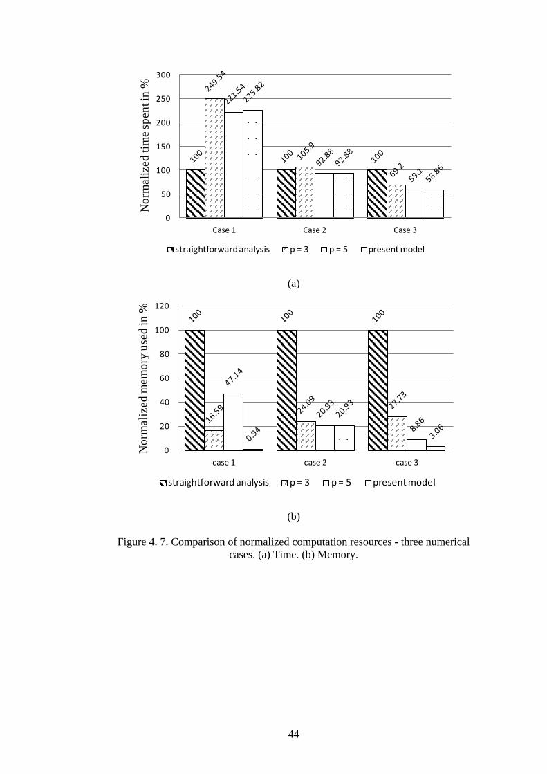
44

(a)

(b)

Figure 4. 7. Comparison of normalized computation resources - three numerical cases. (a) Time. (b) Memory.

0

50

100

150

200

250

300

Case 1 Case 2 Case 3

Nor

mal

ized

tim

e spe

nt in

%

straightforward analysis p = 3 p = 5 present model

0

20

40

60

80

100

120

case 1 case 2 case 3

Nor

mal

ized

mem

ory

used

in %

straightforward analysis p = 3 p = 5 present model

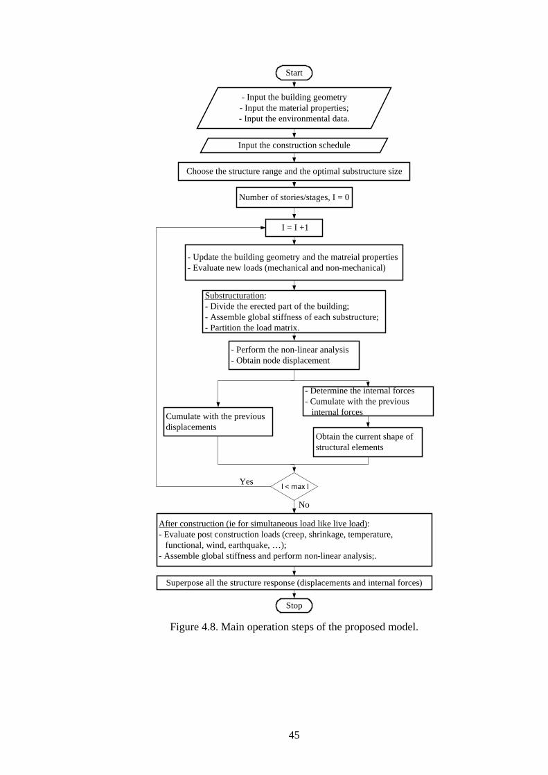
45

Figure 4.8. Main operation steps of the proposed model.

Start

- Input the building geometry- Input the material properties;- Input the environmental data.

Input the construction schedule

Choose the structure range and the optimal substructure size

Number of stories/stages, I = 0

I = I +1

- Update the building geometry and the matreial properties- Evaluate new loads (mechanical and non-mechanical)

Substructuration:- Divide the erected part of the building;- Assemble global stiffness of each substructure;- Partition the load matrix.

- Perform the non-linear analysis- Obtain node displacement

Cumulate with the previous displacements

- Determine the internal forces- Cumulate with the previous internal forces

Obtain the current shape of structural elements

I < max I

After construction (ie for simultaneous load like live load):- Evaluate post construction loads (creep, shrinkage, temperature, functional, wind, earthquake, …);- Assemble global stiffness and perform non-linear analysis;.

Superpose all the structure response (displacements and internal forces)

No

Yes

Stop

46

Chapter 5

NEURAL NETWORK: MINIMIZATION OF

DIFFERENTIAL COLUMN SHORTENING AND

RESULT PREDICTION

Obviously, the SQ-FEA process as presented in the previous chapters, introduced

itself as being much complicated that the conventional analysis which is performed

at one go. But it appears to be more accurate and the computational effort is justified

for detailed phase analysis of a project management. However, for the initial design

phase during which the accuracy is a luxury, structural engineers need to get

structural response easily and quickly with a reasonable approximation. The main

principle is to capture the relationship between simultaneous analysis results and

those of sequential.

Within the framework of this chapter, it has been considered an ANN that aims to

guess directly the erroneous forces between SM-FEA and SQ-FEA. So, just

performing the simultaneous analysis allows the prediction with an acceptable

tolerance of sequential analysis results, differential settlement and forces at the end a

particular beam. Equilibrium equations at different nodes are sufficient to determine

those for columns. In this study, axial forces along beam as well as shear forces for

columns are not investigated since lateral forces applied on building are not

considered.

47

5.1 Neural Network Theory

Human brains are able to complete so sophisticated tasks. To achieve all these, it

is made of about one hundred of billions of neurons

(http://en.wikipedia.org/wiki/Human_brain), nerve cells connected together through

a large network. With the intention to mimic such a system, scientists developed an

artificial neural network composed of processing units. The final result can mainly

perform two specific tasks: pattern recognition and function approximation (Belic,

2012, pp 3-22). This last task is evidently for our concern.

ANN presents several units to the external world arranged in two layers: one for

data input, the other for data output. The input nodes do not process. Sandwiched

between the two external world related layers, there are hidden layers whose

connections to other hidden layers or input/output units are strengthened or

weakened by weights. The actual output out of a given processing unit is the image

of the sum of weighted inputs minus the unit threshold through the activation

function. Herein, output units received zero-value thresholds. Several functions may

act as activation function but they need to be continuous, differentiable,

monotonically non-decreasing and easy to derivate (Fausett, 1994). A typical

function, complying with these requirements, is the bipolar sigmoid function 𝑡𝑎𝑛ℎ(∙)

which will be used for the current problems.

The weights as well as thresholds have to be set along an operation called training

or learning. There are many types of ANN learning algorithm. Walcsak and Cerpa

(1999) claimed that feedforward back propagation algorithm is superior to the others

because of its robustness and its easy accessibility. This algorithm consists of adjust

progressively the weights and thresholds in order to minimize the system energy

based on gradient descent method.

48

After having presented an arbitrary pattern, the energy may be estimated from:

𝐸𝑝 = 12∑ (𝑡𝑘 − 𝑦𝑘)2𝑚𝑘=1 , (5.1)

where 𝑚 is the number of output units, 𝑡 is the target output value and 𝑦 is the actual

output. The minimization of this energy with respect to the network parameters, say

the connection weights and unit thresholds, leads to the updating factors as described

by Rumelhart et al (1986). Plus, it is involved a momentum term used to smooth out

the learning parameter changes. At this step, a given parameter is obtained from

𝑣𝑚 (𝜏 + 1) = 𝑣𝑚(𝜏) − 𝜂 𝜕𝐸𝑝𝜕𝑣𝑚

+ 𝛼 𝛥𝑣𝑚(𝜏), (5 2)

in which 𝑣𝑚 is the parameter under optimization, 𝜏 is the counter of the learning

process, 𝜂 is the gain fraction, 𝛼 is the momentum term, and 𝛥𝑣𝑚(𝜏) = 𝑣𝑚(𝜏) −

𝑣𝑚(𝜏 − 1).

As a supervised paradigm, all the input/output patterns of the training set should

be presented to the network during the learning phase. One epoch designates a

complete passage throughout the whole training set. The number of epochs may be

used to characterize the learning process. It is necessary to precondition the patterns

to have good performance. The input variables are scaled between [-1, 1] so that their

respective mean values should be close to zero or else small compared to their

respective standard deviation (Haykin, 2005) and the output are preprocessed to be

within the range of the activation function avoiding saturation (Haykin, 2005; Belic,

2012).

5.2 Minimization of Differential Column Shortening

Choi and Kim (1985) and Choi et al (1992) remarked that the different tributary

areas which exterior and interior column support, generate different loads upon these

columns, approximately the double for internal columns. Since external columns are

also robustly designed to withstand lateral forces, their shortening is moderate

49

compared to those of internal ones. This causes differential column shortenings in

buildings. According to Fintel, Ghosh, and Iyengar (1986), the immediate

consequence results in damages on non structural elements such as partitions

especially light ones, architecture finishes and built-in furnishings, mechanical

equipments and cladding. Also, the functionality and the visual aspect may be

concerned. Wherefore, it is important to reduce this differential settlement.

5.2.1 Overview

Many factors characterize a particular project. These factors determine the

structural response amongst which, displacements. Impacting on these displacements

necessarily passes through the judicious adjustment of the relevant factors:

environment, structure geometry and materials, and construction process.

Environmental factors concern mainly temperature and relative humidity which are

difficult to influence on. The general geometry of the edifice and members’ sizes are

dictated by the architectural and structural design. Generally, the material

specifications to be used, say cement type and concrete grade, are specified in the

tender documents or guided by the availability in the project location. The

construction process, especially the interphase period between two typical stages, has

a great impact on the total duration of the project, and, thus, on the total cost.

Haroglu et al (2009) claimed that it is the structural engineer who is the most

influential in selecting the correct structural frame for a project’s feasibility and

success. Therefore, he should propose a typical duration characterizing the

construction timing. In short, it is convenient to minimize the differential shortening

by choosing a suitable elementary duration since the other factors are awkward to be

imposed or modified.

50

By considering a very short period of time between two stages, the concrete is still

weak when receiving loads, and, thus, is much subjected to instantaneous

deformations. On the other hand, if one waits too much between two stages, he

allows temperature to change a lot and induces more stresses across the members.

Here, the daily variations on temperature are considered negligible since they are

generally small and they do not have enough time to penetrate across member’s

sections. Also, a high amount of temperature change may cause more shrinkage

effects. By increasing internal forces and keeping for a long period of time

construction loads applied on story below, one will result in more instantaneous

deformations and more creep effects over the lengthy phase. Obviously, there is an

optimal interphase between these two extreme cases that yields to a minimum

maximorum differential shortening; since it is suitable to minimize the differential

shortening at the member location it is more critical.

5.2.2 Illustrative Example

The same L-shaped 15-story office building of Section 3.3.1 is held here. But

now, the elasticity modulus at 28 days has been obtained from Section 2.5.3 of the

present thesis and became 𝐸𝐶(28) = 27 050 𝑀𝑃𝑎.

Different analyses have been made with the commercial structural analysis

software package SAP2000 version 15.1.0. The interphase has been varied from 1 to

28 days. That is, for a given interphase, the analysis has been conducted and the

maximum differential column shortening has been noted as result. The graph in

Figure 5.1 represents the evolution of the maximum differential shortening versus the

interphase. It readily appears that the minimum occurs for the critical interphase of

10 days.

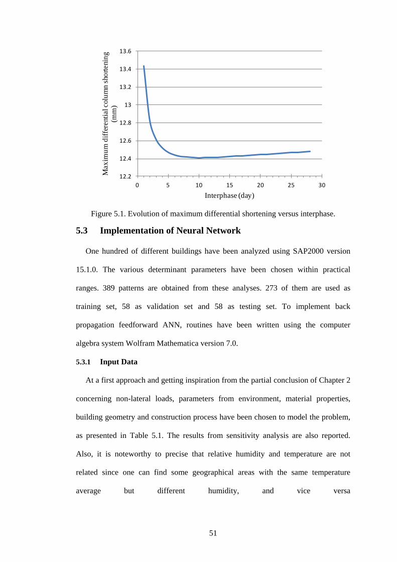
51

Figure 5.1. Evolution of maximum differential shortening versus interphase.

5.3 Implementation of Neural Network

One hundred of different buildings have been analyzed using SAP2000 version

15.1.0. The various determinant parameters have been chosen within practical

ranges. 389 patterns are obtained from these analyses. 273 of them are used as

training set, 58 as validation set and 58 as testing set. To implement back

propagation feedforward ANN, routines have been written using the computer

algebra system Wolfram Mathematica version 7.0.

5.3.1 Input Data

At a first approach and getting inspiration from the partial conclusion of Chapter 2

concerning non-lateral loads, parameters from environment, material properties,

building geometry and construction process have been chosen to model the problem,

as presented in Table 5.1. The results from sensitivity analysis are also reported.

Also, it is noteworthy to precise that relative humidity and temperature are not

related since one can find some geographical areas with the same temperature

average but different humidity, and vice versa

12.2

12.4

12.6

12.8

13

13.2

13.4

13.6

0 5 10 15 20 25 30

Max

imum

diff

eren

tial c

olum

n sh

orte

ning

(m

m)

Interphase (day)

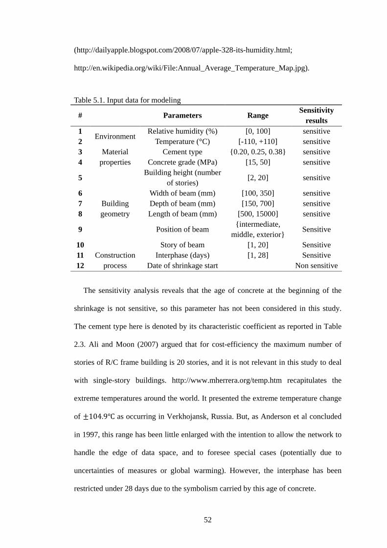
52

(http://dailyapple.blogspot.com/2008/07/apple-328-its-humidity.html;

http://en.wikipedia.org/wiki/File:Annual_Average_Temperature_Map.jpg).

Table 5.1. Input data for modeling

# Parameters Range Sensitivity results

1 Environment Relative humidity (%) [0, 100] sensitive

2 Temperature (°C) [-110, +110] sensitive 3 Material

properties Cement type {0.20, 0.25, 0.38} sensitive

4 Concrete grade (MPa) [15, 50] sensitive

5

Building geometry

Building height (number of stories)

[2, 20] sensitive

6 Width of beam (mm) [100, 350] sensitive 7 Depth of beam (mm) [150, 700] sensitive 8 Length of beam (mm) [500, 15000] sensitive

9 Position of beam {intermediate,

middle, exterior} Sensitive

10 Story of beam [1, 20] Sensitive 11 Construction

process Interphase (days) [1, 28] Sensitive

12 Date of shrinkage start Non sensitive

The sensitivity analysis reveals that the age of concrete at the beginning of the

shrinkage is not sensitive, so this parameter has not been considered in this study.

The cement type here is denoted by its characteristic coefficient as reported in Table

2.3. Ali and Moon (2007) argued that for cost-efficiency the maximum number of

stories of R/C frame building is 20 stories, and it is not relevant in this study to deal

with single-story buildings. http://www.mherrera.org/temp.htm recapitulates the

extreme temperatures around the world. It presented the extreme temperature change

of ±104.9℃ as occurring in Verkhojansk, Russia. But, as Anderson et al concluded

in 1997, this range has been little enlarged with the intention to allow the network to

handle the edge of data space, and to foresee special cases (potentially due to

uncertainties of measures or global warming). However, the interphase has been

restricted under 28 days due to the symbolism carried by this age of concrete.

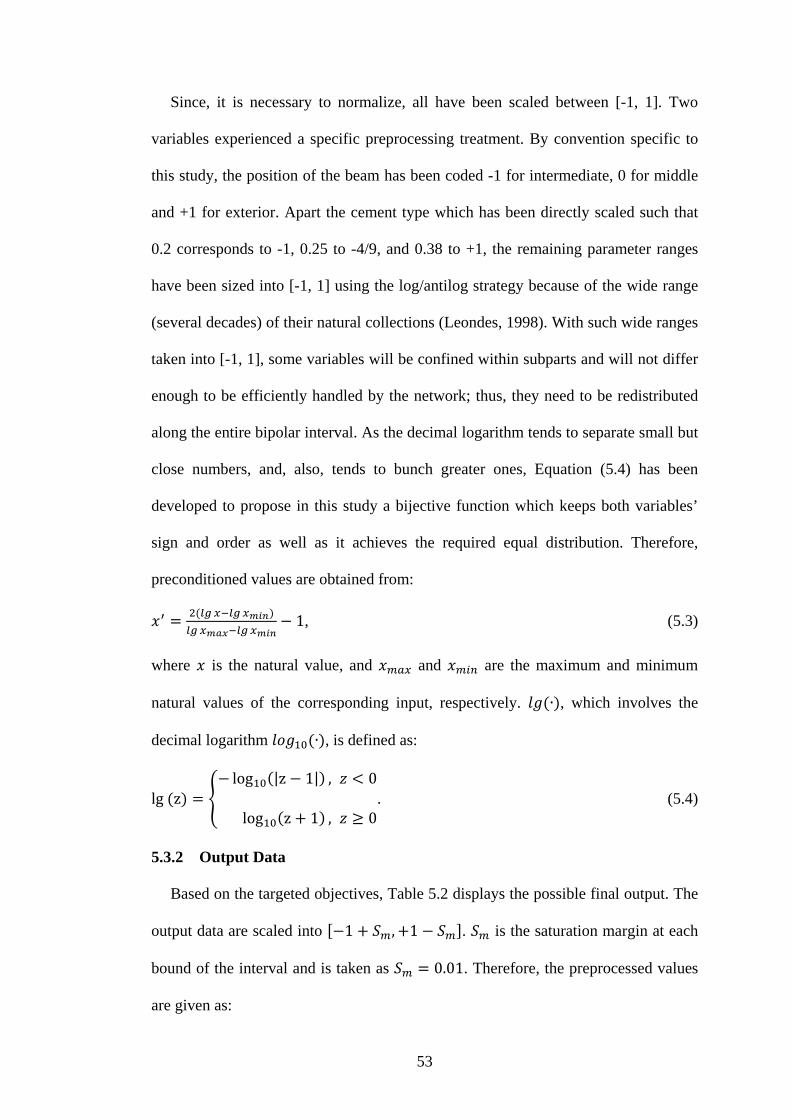
53

Since, it is necessary to normalize, all have been scaled between [-1, 1]. Two

variables experienced a specific preprocessing treatment. By convention specific to

this study, the position of the beam has been coded -1 for intermediate, 0 for middle

and +1 for exterior. Apart the cement type which has been directly scaled such that

0.2 corresponds to -1, 0.25 to -4/9, and 0.38 to +1, the remaining parameter ranges

have been sized into [-1, 1] using the log/antilog strategy because of the wide range

(several decades) of their natural collections (Leondes, 1998). With such wide ranges

taken into [-1, 1], some variables will be confined within subparts and will not differ

enough to be efficiently handled by the network; thus, they need to be redistributed

along the entire bipolar interval. As the decimal logarithm tends to separate small but

close numbers, and, also, tends to bunch greater ones, Equation (5.4) has been

developed to propose in this study a bijective function which keeps both variables’

sign and order as well as it achieves the required equal distribution. Therefore,

preconditioned values are obtained from:

𝑥′ = 2(𝑙𝑔 𝑥−𝑙𝑔 𝑥𝑚𝑖𝑛)𝑙𝑔 𝑥𝑚𝑎𝑥−𝑙𝑔 𝑥𝑚𝑖𝑛

− 1, (5.3)

where 𝑥 is the natural value, and 𝑥𝑚𝑎𝑥 and 𝑥𝑚𝑖𝑛 are the maximum and minimum

natural values of the corresponding input, respectively. 𝑙𝑔(∙), which involves the

decimal logarithm 𝑙𝑜𝑔10(∙), is defined as:

lg (z) = �− log10(|z − 1|) , 𝑧 < 0

log10(z + 1) , 𝑧 ≥ 0�. (5.4)

5.3.2 Output Data

Based on the targeted objectives, Table 5.2 displays the possible final output. The

output data are scaled into [−1 + 𝑆𝑚, +1 − 𝑆𝑚]. 𝑆𝑚 is the saturation margin at each

bound of the interval and is taken as 𝑆𝑚 = 0.01. Therefore, the preprocessed values

are given as:

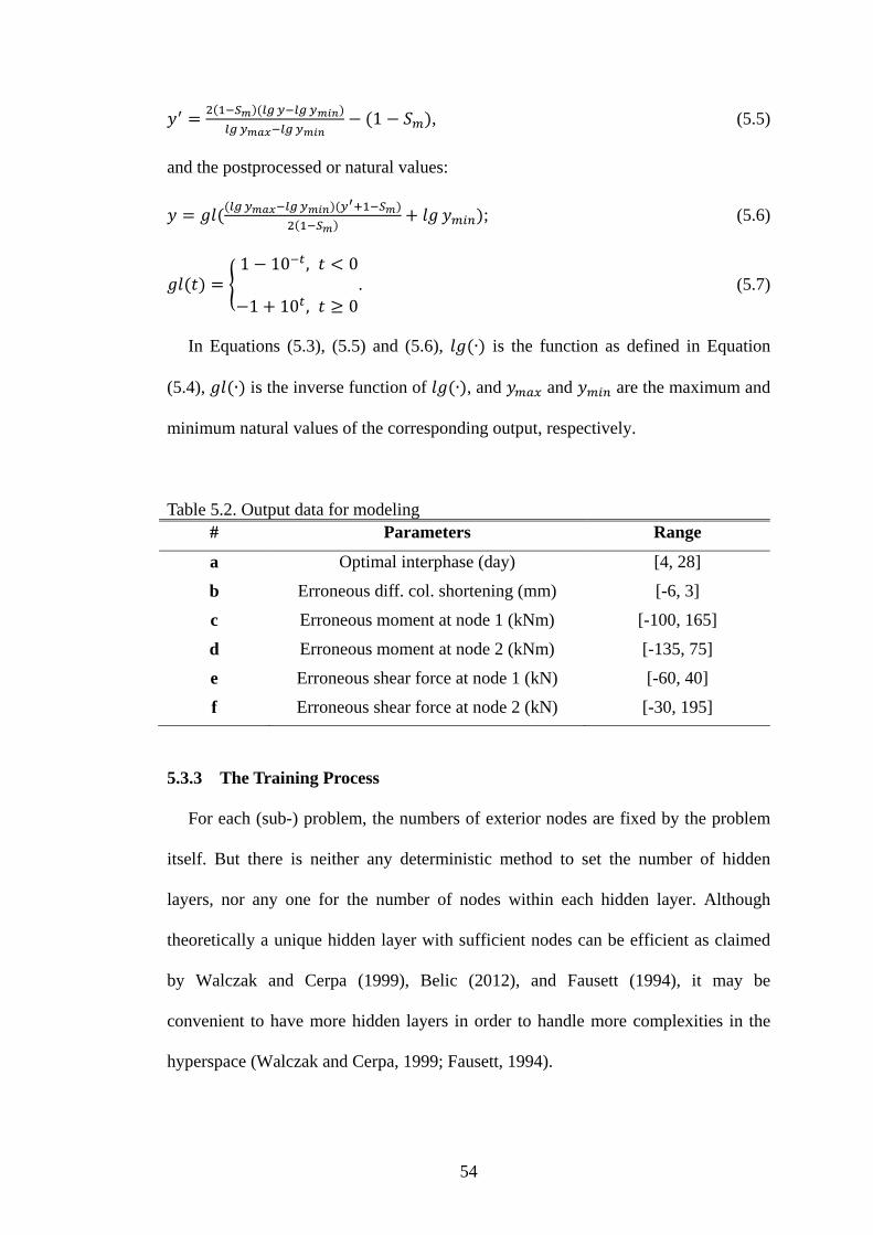
54

𝑦′ = 2(1−𝑆𝑚)(𝑙𝑔 𝑦−𝑙𝑔𝑦𝑚𝑖𝑛)𝑙𝑔 𝑦𝑚𝑎𝑥−𝑙𝑔𝑦𝑚𝑖𝑛

− (1 − 𝑆𝑚), (5.5)

and the postprocessed or natural values:

𝑦 = 𝑔𝑙((𝑙𝑔 𝑦𝑚𝑎𝑥−𝑙𝑔𝑦𝑚𝑖𝑛)(𝑦′+1−𝑆𝑚)2(1−𝑆𝑚)

+ 𝑙𝑔 𝑦𝑚𝑖𝑛); (5.6)

𝑔𝑙(𝑡) = �1 − 10−𝑡 , 𝑡 < 0

−1 + 10𝑡 , 𝑡 ≥ 0�. (5.7)

In Equations (5.3), (5.5) and (5.6), 𝑙𝑔(∙) is the function as defined in Equation

(5.4), 𝑔𝑙(∙) is the inverse function of 𝑙𝑔(∙), and 𝑦𝑚𝑎𝑥 and 𝑦𝑚𝑖𝑛 are the maximum and

minimum natural values of the corresponding output, respectively.

Table 5.2. Output data for modeling # Parameters Range

a Optimal interphase (day) [4, 28]

b Erroneous diff. col. shortening (mm) [-6, 3]

c Erroneous moment at node 1 (kNm) [-100, 165]

d Erroneous moment at node 2 (kNm) [-135, 75]

e Erroneous shear force at node 1 (kN) [-60, 40]

f Erroneous shear force at node 2 (kN) [-30, 195]

5.3.3 The Training Process

For each (sub-) problem, the numbers of exterior nodes are fixed by the problem

itself. But there is neither any deterministic method to set the number of hidden

layers, nor any one for the number of nodes within each hidden layer. Although

theoretically a unique hidden layer with sufficient nodes can be efficient as claimed

by Walczak and Cerpa (1999), Belic (2012), and Fausett (1994), it may be

convenient to have more hidden layers in order to handle more complexities in the

hyperspace (Walczak and Cerpa, 1999; Fausett, 1994).

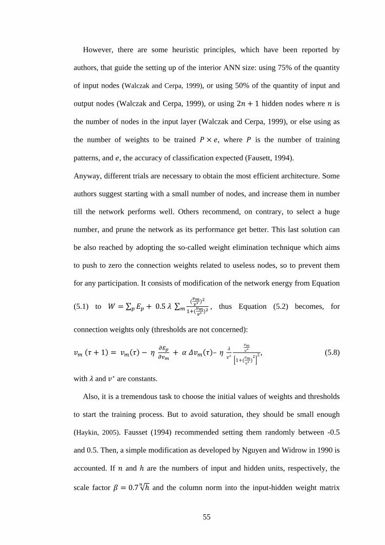
55

However, there are some heuristic principles, which have been reported by

authors, that guide the setting up of the interior ANN size: using 75% of the quantity

of input nodes (Walczak and Cerpa, 1999), or using 50% of the quantity of input and

output nodes (Walczak and Cerpa, 1999), or using 2𝑛 + 1 hidden nodes where 𝑛 is

the number of nodes in the input layer (Walczak and Cerpa, 1999), or else using as

the number of weights to be trained 𝑃 × 𝑒, where 𝑃 is the number of training

patterns, and 𝑒, the accuracy of classification expected (Fausett, 1994).

Anyway, different trials are necessary to obtain the most efficient architecture. Some

authors suggest starting with a small number of nodes, and increase them in number

till the network performs well. Others recommend, on contrary, to select a huge

number, and prune the network as its performance get better. This last solution can

be also reached by adopting the so-called weight elimination technique which aims

to push to zero the connection weights related to useless nodes, so to prevent them

for any participation. It consists of modification of the network energy from Equation

(5.1) to 𝑊 = ∑ 𝐸𝑝 + 0.5 𝜆 ∑(𝑣𝑚𝑣∗ )2

1+(𝑣𝑚𝑣∗ )2𝑚 𝑝 , thus Equation (5.2) becomes, for

connection weights only (thresholds are not concerned):

𝑣𝑚 (𝜏 + 1) = 𝑣𝑚(𝜏) − 𝜂 𝜕𝐸𝑝𝜕𝑣𝑚

+ 𝛼 𝛥𝑣𝑚(𝜏)– 𝜂 𝜆𝑣∗

𝑣𝑚𝑣∗

�1+(𝑣𝑚𝑣∗ )2�

2 , (5.8)

with 𝜆 and 𝑣∗ are constants.

Also, it is a tremendous task to choose the initial values of weights and thresholds

to start the training process. But to avoid saturation, they should be small enough

(Haykin, 2005). Fausset (1994) recommended setting them randomly between -0.5

and 0.5. Then, a simple modification as developed by Nguyen and Widrow in 1990 is

accounted. If 𝑛 and ℎ are the numbers of input and hidden units, respectively, the

scale factor 𝛽 = 0.7√ℎ𝑛 and the column norm into the input-hidden weight matrix

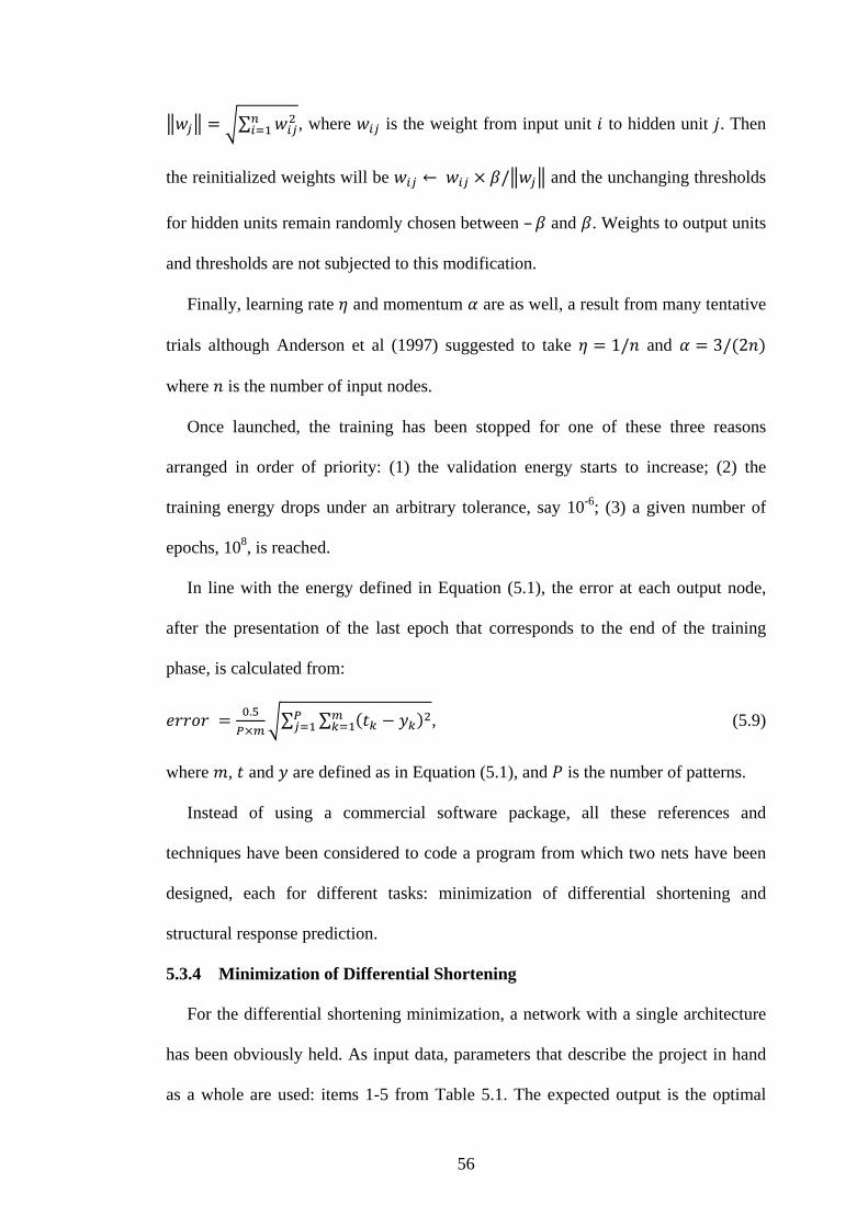
56

�𝑤𝑗� = �∑ 𝑤𝑖𝑗2𝑛𝑖=1 , where 𝑤𝑖𝑗 is the weight from input unit 𝑖 to hidden unit 𝑗. Then

the reinitialized weights will be 𝑤𝑖𝑗 ← 𝑤𝑖𝑗 × 𝛽/�𝑤𝑗� and the unchanging thresholds

for hidden units remain randomly chosen between –𝛽 and 𝛽. Weights to output units

and thresholds are not subjected to this modification.

Finally, learning rate 𝜂 and momentum 𝛼 are as well, a result from many tentative

trials although Anderson et al (1997) suggested to take 𝜂 = 1/𝑛 and 𝛼 = 3/(2𝑛)

where 𝑛 is the number of input nodes.

Once launched, the training has been stopped for one of these three reasons

arranged in order of priority: (1) the validation energy starts to increase; (2) the

training energy drops under an arbitrary tolerance, say 10-6; (3) a given number of

epochs, 108, is reached.

In line with the energy defined in Equation (5.1), the error at each output node,

after the presentation of the last epoch that corresponds to the end of the training

phase, is calculated from:

𝑒𝑟𝑟𝑜𝑟 = 0.5𝑃×𝑚�∑ ∑ (𝑡𝑘 − 𝑦𝑘)2𝑚

𝑘=1𝑃𝑗=1 , (5.9)

where 𝑚, 𝑡 and 𝑦 are defined as in Equation (5.1), and 𝑃 is the number of patterns.

Instead of using a commercial software package, all these references and

techniques have been considered to code a program from which two nets have been

designed, each for different tasks: minimization of differential shortening and

structural response prediction.

5.3.4 Minimization of Differential Shortening

For the differential shortening minimization, a network with a single architecture

has been obviously held. As input data, parameters that describe the project in hand

as a whole are used: items 1-5 from Table 5.1. The expected output is the optimal

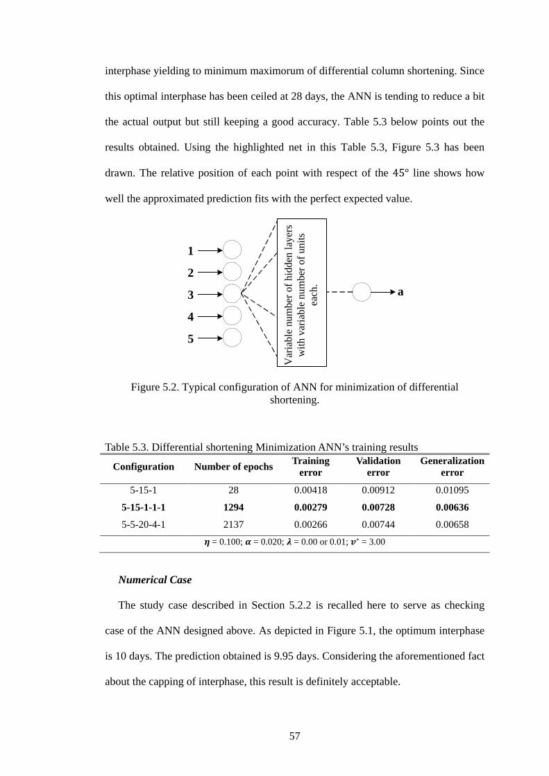
57

interphase yielding to minimum maximorum of differential column shortening. Since

this optimal interphase has been ceiled at 28 days, the ANN is tending to reduce a bit

the actual output but still keeping a good accuracy. Table 5.3 below points out the

results obtained. Using the highlighted net in this Table 5.3, Figure 5.3 has been

drawn. The relative position of each point with respect of the 45° line shows how

well the approximated prediction fits with the perfect expected value.

Figure 5.2. Typical configuration of ANN for minimization of differential shortening.

Table 5.3. Differential shortening Minimization ANN’s training results

Configuration Number of epochs Training error

Validation error

Generalization error

5-15-1 28 0.00418 0.00912 0.01095

5-15-1-1-1 1294 0.00279 0.00728 0.00636

5-5-20-4-1 2137 0.00266 0.00744 0.00658

𝜼 = 0.100; 𝜶 = 0.020; 𝝀 = 0.00 or 0.01; 𝒗∗ = 3.00

Numerical Case

The study case described in Section 5.2.2 is recalled here to serve as checking

case of the ANN designed above. As depicted in Figure 5.1, the optimum interphase

is 10 days. The prediction obtained is 9.95 days. Considering the aforementioned fact

about the capping of interphase, this result is definitely acceptable.

Var

iabl

e nu

mbe

r of h

idde

n la

yers

w

ith v

aria

ble

num

ber o

f uni

ts

each

.

1

2

3

4

5

a

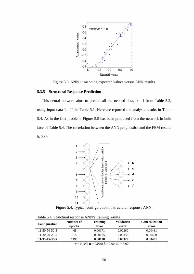
58

Figure 5.3. ANN 1: mapping expected values versus ANN results.

5.3.5 Structural Response Prediction

This neural network aims to predict all the needed data, b – f from Table 5.2,

using input data 1 - 11 in Table 5.1. Here are reported the analysis results in Table

5.4. As in the first problem, Figure 5.5 has been produced from the network in bold

face of Table 5.4. The correlation between the ANN prognostics and the FEM results

is 0.89.

Figure 5.4. Typical configuration of structural response ANN.

Table 5.4. Structural response ANN’s training results

Configuration Number of

epochs Training

error Validation

error Generalization

error 11-50-50-50-5 468 0.00171 0.00360 0.00431 11-20-20-20-5 915 0.00175 0.00338 0.00460 11-35-45-35-5 1198 0.00138 0.00329 0.00431

𝜼 = 0.100; 𝜶 = 0.020; 𝝀 = 0.00; 𝒗∗ = 3.00

correlation = 0.98

1.0 0.5 0.0 0.5 1.00.6

0.4

0.2

0.0

0.2

0.4

0.6

0.8

Expected valuesAp

prox

imate

dva

lues

1

2

3

4

5

6

7

8

9

10

11

Var

iabl

e nu

mbe

r of h

idde

n la

yers

with

var

iabl

e nu

mbe

r of u

nits

eac

h. b

c

d

e

f

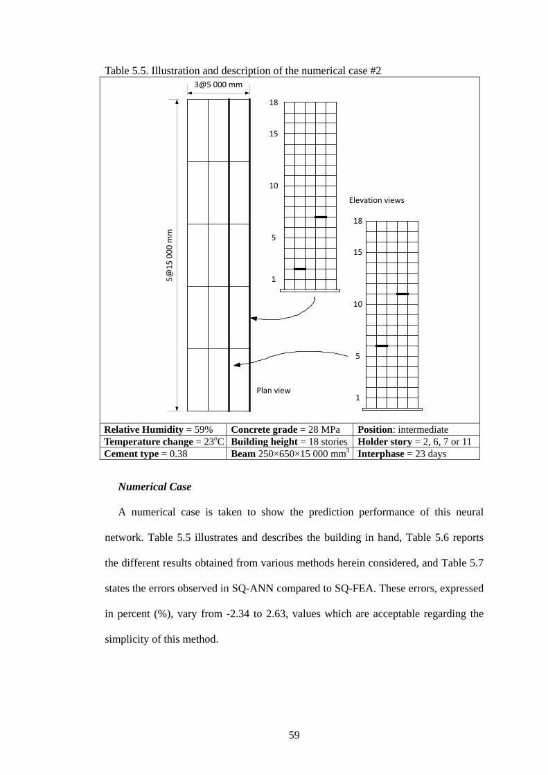
59

Table 5.5. Illustration and description of the numerical case #2

Relative Humidity = 59% Concrete grade = 28 MPa Position: intermediate Temperature change = 23oC Building height = 18 stories Holder story = 2, 6, 7 or 11 Cement type = 0.38 Beam 250×650×15 000 mm3 Interphase = 23 days

Numerical Case

A numerical case is taken to show the prediction performance of this neural

network. Table 5.5 illustrates and describes the building in hand, Table 5.6 reports

the different results obtained from various methods herein considered, and Table 5.7

states the errors observed in SQ-ANN compared to SQ-FEA. These errors, expressed

in percent (%), vary from -2.34 to 2.63, values which are acceptable regarding the

simplicity of this method.

1

18

15

10

5

1

18

15

10

5

5@15

000

mm

3@5 000 mm

Plan view

Elevation views

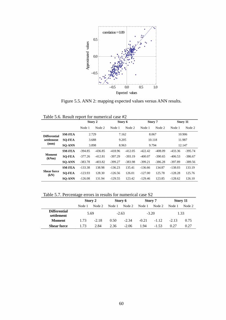
60

Figure 5.5. ANN 2: mapping expected values versus ANN results.

Table 5.6. Result report for numerical case #2 Story 2 Story 6 Story 7 Story 11

Node 1 Node 2 Node 1 Node 2 Node 1 Node 2 Node 1 Node 2

Differential settlement

(mm)

SM-FEA 2.729 7.162 8.067 10.906

SQ-FEA 3.688 9.205 10.118 11.987

SQ-ANN 3.898 8.963 9.794 12.147

Moment (kNm)

SM-FEA -394.85 -436.85 -418.96 -412.05 -422.42 -408.09 -433.36 -395.74

SQ-FEA -377.26 -412.81 -397.29 -393.19 -400.07 -390.65 -406.53 -386.67

SQ-ANN -383.78 -403.82 -399.27 -383.98 -399.21 -386.28 -397.89 -389.56

Shear force (kN)

SM-FEA -133.38 138.98 -136.23 135.41 -136.66 134.87 -138.03 133.19

SQ-FEA -123.93 128.30 -126.56 126.01 -127.00 125.78 -128.28 125.76

SQ-ANN -126.08 131.94 -129.55 123.42 -129.46 123.85 -128.62 126.10

Table 5.7. Percentage errors in results for numerical case S2

Story 2 Story 6 Story 7 Story 11

Node 1 Node 2 Node 1 Node 2 Node 1 Node 2 Node 1 Node 2 Differential settlement 5.69 -2.63 -3.20 1.33

Moment 1.73 -2.18 0.50 -2.34 -0.21 -1.12 -2.13 0.75 Shear force 1.73 2.84 2.36 -2.06 1.94 -1.53 0.27 0.27

correlation = 0.89

0.5 0.0 0.5 1.0

0.5

0.0

0.5

Expected valuesAp

prox

imate

dva

lues

61

Chapter 6

CONCLUSION AND RECOMMENDATIONS

6.1 Summary

Throughout this thesis, many problematics have been considered around

sequential analysis. The first one was the presentation of this theory and the

highlighting of its significance. Here, a strategy on how to conduct this analysis has

been proposed, considering the realistic situation under which actual R/C 3D frames

building are subjected including various common loads. The individual contributions

of these loads have been investigated on a study case, not each separately, but

sequentially as they are applied in situ.

The second problem dealt with an accurate process aiming to reduce the

computational resources required to perform sequential analysis, say memory and

time. The substructuring technique as proposed as Przemieniecki (1968) has been

reformulated and coupled to sequential analysis without any loss of accuracy.

Since sequential analysis is firmly related to differential column shortening

phenomenon, the third goal aimed to reduce it by a carefully selection the interphase

that leads to minimum maximorum differential column shortening. For this purpose,

an artificial neural network has been designed; it takes as inputs general and easy-to-

get project’s parameters and brings out the said optimal interphase. Another artificial

neural network has been put up with the intention to predict sequential analysis

results from those of simultaneous one. It has been found out that these tools are

useful at the preliminary design stage.

62

6.2 Conclusion

After peeling out various loads, findings are alarming. These following major

lines can be stated.

• For beams located at lower floor, SQ-FEA’s and SM-FEA’s moments are not

divergent, but they are for upper floor where a 62% difference can be observed.

• SQ-FEA results show that moments are actually more distributed along

continuous beams than SM-FEA seems to demonstrate.

• The difference between the two analyses is more sensitive with irregularities in

buildings.

• This difference is moderated when applying live load.

• Temperature actions happened to be of great importance for the lower stories

where a change of 50% can be noticed in the second floor, and a different

behavior may arise in the first one since the moment’s sign may be inversed,

from -65.36 kNm to +14.49 kNm for example. Although their effect can be

neglected for the upper stories, the final moment curve is more influenced, even

dictated, by the temperature curve when it is considered.

• From top to bottom, time dependent effect and construction loads induce greater

change on moments computed when they are ignored. Altogether, they may

equally share a change in moments of 65%.

• Earthquake action does not significantly vary from one analysis to another.

These points prove that, when statically analyzing a building, the nonlinearity

caused by the sequential application of loads has to be accounted. Furthermore, all

the various loads investigated here happened to play great role such that there will be

a serious default if not.

63

Nevertheless, SQ-FEA required computational consuming process. To overcome

this problem, an algorithm has been proposed to help engineers to easily implement

this process in an optimal manner. From the statistical analysis of the experiments

which coupled sequential analysis and substructuring technique, the result has been

the conception of a simple process based on the choice of the optimal substructure

size. With the study cases that have been considered, up to 42.14% of time amount

and 99.06% of memory amount have been saved.

But this is still tedious when the full accuracy is not required. A soft computing

tool, well known as artificial neural network, has been used here to cope this case.

Instead of using a commercial software package, many references providing

advanced principles have been considered to code a program. Without any analysis,

but just by considering five general parameters to characterize a given project, the

optimal interphase can be predicted with a very short time computation.

In addition, in order to avoid repeated analyses required by sequential analysis,

whose procedure demands intricate modeling and long waiting time of analysis, its

results can be deducted from those of simultaneous one by the means of another

ANN. For one or the other, errors have been kept under 0.01 and correlation above

0.89. ANNs exempt engineers from full structure modeling for each change and/or

analysis, but offer an acceptable accuracy in results by a second-duration

computation.

6.3 Recommendation for Further Works

The sizing procedure developed here for substructuring considers only gravity

loads occurring during the construction phase. It may be important to extend it to all

the various loads. Also, it has been proposed based on regular rectangular 3D frames,

further studies can investigate the case of vertically irregular ones.

64

The database which has been used for neural network training and validation,

concerned only residential / office buildings with neither vertical irregularity nor

circular part. Other networks can be set up considering these features.

In addition, training and validation sets have been chosen only amongst R/C

buildings. Other constituting materials such as steel, prestressed concrete, or timber

could be accounted to extend the range of these networks.

65

REFERENCES

Ali MM, & Moon KS. (2007). Structural developments in tall buildings: current

trends and future prospects. Architecture Science Review. 50 (3), 205-23.

Anderson D, Hines EL, Arthur SJ, & Eiap EL. (1997). Application of artificial neural

network to prediction of minor steel connections. Structures & Computers. 63(4),

685-92.

Association Française de la NORmalisation. Eurocode 1 : “Bases de Calculs et

Actions sur les Structures” et Documents d’Application Nationale. AFNOR

2000. Tour Europe 92049 Paris La Défense Cedex.

Association Française de la NORmalisation. Eurocode 8 : Conception et

dimensionnement des structures pour leur résistance aux séismes et documents

d’application nationale. Partie 1. AFNOR 2000. Tour Europe 92049 Paris La

Défense Cedex.

Azkune M, Puente I, & Insausti A. (2007). Effect of ambient temperature on the

redistribution of loads during construction of multi-storey concrete structures.

Engineering Structures. 29, 933-41.

Ballal TMA, & Sher WD. (2003). Artificial neural network for the selection of

buildable structural systems. Engineering, Construction and architectural

management. 10 (4): 263-71.

66

Belic I. (2012). Neural networks and static modeling. In: ElHefnawi M, Mysara M,

editors. Recurrent neural networks and soft computing. Croatia: InTech. p. 3-22.

Choi CK, Chung HK, Lee DG, & Wilson EL. (1992). Simplified building analysis

with sequential dead loads-CFM. Journal of Structural Engineering ASCE.

118(4), 944-54.

Choi CK, & Kim ED. (1985). Multistory frames under sequential gravity loads.

Journal of Structural Engineering ASCE. 111(11), 2373-84.

Comite Euro-International du Beton. (1993). CEB-FIP Model Code 1990, Design

Code. London: Thomas Telford Services Ltd.

Fausett L. (1994). Fundamentals of neural networks: architectures, algorithms and

applications. New Jersey: Prentice-Hall.

Fintel M, Ghosh SK, & Iyengar H. (1986). Column shortening in tall structures –

prediction and compensation. Portland cement association.

Fu XY, Wu B, Chen XC, Meng ML, Sun C, Jiang HB, Gao Y, & Li JW. (2008).

Research on structural design of a super high-rise building in Qatar. The IES

Journal Part A: Civil & Structural Engineering. 1(3), 186-97.

Gupta T, & Sharma RK. (2011). Structural analysis and design of building using

neural network: a review. International Journal of Engineering and Management

Sciences. 2(4), 216-20.

67

Haroglu H, Glass J, Thorpe T, & Goodchild C. (2009). Who is the key decision

maker in the structural frame selection process? In: Limbachiya, Kew, editors.

Excellence in concrete construction through innovation. England: Taylor &

Francis Group. p. 119-26.

Haykin S. (2005). Neural network – A comprehensive foundation. 2nd ed. India:

Pearson Education Inc.

He Y, Zhou X, & Hou P. (2010). Combined method of super element and

substructure for analysis of ILTDBS reticulated mega-structure with single-layer

latticed shell substructures. Finite Elements in Analysis and Design. 46, 563-70.

http://dailyapple.blogspot.com/2008/07/apple-328-its-humidity.html. Last accessed

on August 10th, 2012.

http://en.wikipedia.org/wiki/File:Annual_Average_Temperature_Map.jpg. Last

accessed on August 10th, 2012.

http://en.wikipedia.org/wiki/Human_brain. Last accessed on August 10th, 2012.

http://www.climatetemp.info/cyprus/famagusta.html. Last accessed on March 09th,

2012.

http://www.mherrera.org/temp.htm. Last accessed on August 10th, 2012.

68

Iliadis L, & Jayne C, editors. (2011). Engineering applications of neural networks.

Part 1. London: Springer.

Kim HS, & Shin SH. (2011). Column shortening analysis with lumped construction

sequences. Procedia Engineering. 14, 1791-98.

Kwak HG, & Kim JK. (2006). Time-dependent analysis of RC frame structures

considering construction sequences. Building and Environment. 41, 1423-34.

Leondes CT. (1998). Optimization techniques. California: Academic Press.

Leung YT. (1979). An accurate method of dynamic substructuring with simplified

computation. International Journal for Numerical Methods in Engineering.

14:1241-56.

Liu NX, Zhao X, Sun HH, Zheng YM, & Ding JM. (2011). Structural performance

assessment and control of super tall buildings during construction. Procedia

Engineering. 14, 2503-10.

Rumelhart DE, Hinton GE, & Williams RJ. (1986). Learning internal representations by

error propagation. In: Parallel Distributed Processing Vol. 1: Foundations. The MIT

Press, MA.

Solomos G, Pinto A, & Dimova S. (2008). A Review of the Seismic Hazard

Zonation in National Building Codes in the Context of Euro code 8.

Luxembourg: Office for Official Publications of the European Communities.

69

Ozay G, & Njomo W. (2012a). Minimization of differential column shortening and

sequential analysis of RC 3D-frame using ANN. Structural Engineering and

Mechanics (submitted for review).

Ozay G, & Njomo W. (2012b). Sequential analysis coupled with optimized

substructure technique on 3D-frame construction process. Engineering

Structures. (submitted for review).

Przemieniecki JS. (1963). Matrix structural analysis of substructures. J. Am. Inst.

Aeron. Astron. 1,138-47.

Przemieniecki JS. (1968). Theory of matrix structural analysis. New York: McGraw-

Hill Book Company.

Walczak S, & Cerpa N. (1999). Heuristic principles for the design of artificial neural

networks. Information and software technology. 41, 107-17.