Sequencing dual-spreader crane operations: Mathematicalformulation and heuristic algorithm

Author

Lashkari, Shabnam, Wu, Yong, Petering, Matthew EH

Published

2017

Journal Title

European Journal of Operational Research

Version

Accepted Manuscript (AM)

DOI

https://doi.org/10.1016/j.ejor.2017.03.046

Copyright Statement

© 2017 Elsevier. Licensed under the Creative Commons Attribution-NonCommercial-NoDerivatives 4.0 International (http://creativecommons.org/licenses/by-nc-nd/4.0/) whichpermits unrestricted, non-commercial use, distribution and reproduction in any medium,providing that the work is properly cited.

Downloaded from

http://hdl.handle.net/10072/347178

Griffith Research Online

https://research-repository.griffith.edu.au

Sequencing dual-spreader crane operations:

Mathematical formulation and heuristic algorithm

Shabnam Lashkaria, Yong Wub, Matthew E. H. Peteringa,∗

aDepartment of Industrial and Manufacturing Engineering, University ofWisconsin–Milwaukee, P.O. Box 784, Milwaukee, WI 53201, USA

bDepartment of International Business and Asian Studies, Griffith University, GoldCoast Campus, QLD 4222 Australia

Abstract

This paper investigates the problem of scheduling a dual-spreader crane whenlifts are subject to a weight limit. A mathematical model is formulatedand a fast method for computing a lower bound on the optimal value isproposed. An efficient heuristic approach is designed and subsequently builtinto a simulated annealing framework to solve the problem. The optimizationand heuristic approaches are tested on problem instances of various sizes.The results indicate that the optimization approach produces proven optimalsolutions to small-sized instances but fails to solve instances of practicalmeaning. The heuristic approach can easily match the performance of theoptimization approach for small instances and outperforms the optimizationapproach when tackling larger instances. On average, the heuristic approachproduces solutions whose objective values are within 6% of the lower bound.

Keywords: dual-spreader crane, tandem-lift crane, integer programming,heuristics, planning and scheduling, container terminal, quay crane

1. Introduction

Today most overseas shipping of finished consumer goods is done via 20-,40-, or 45-foot long steel containers aboard deep-sea container vessels. Inaddition, the amount of meat, fish, fruit, vegetables, and general foodstuffs

∗Corresponding author. Tel: +1-414-229-3448, fax: +1-414-229-6958.Email addresses: lashkari@uwm.edu (Shabnam Lashkari),

yong.wu@griffith.edu.au (Yong Wu), mattpete@uwm.edu (Matthew E. H. Petering)

Preprint submitted to European Journal of Operational Research September 16, 2016

Figure 1: Double-spreader crane in operation (Source: http://www.portstrategy.com/news101/port-operations/cargo-handling/multilift_for_and_against, accessedon 27 November 2015.)

shipped in refrigerated containers continues to increase. As the volume offreight shipped via steel shipping containers grows, it is becoming increasinglyimportant to improve the operational efficiency of the port facilities wherecontainerships are unloaded and loaded.

In this paper, we introduce a new mathematical problem that is inspiredby the unloading of a containership. This problem is inspired by the recentdevelopment of a new kind of quay crane—a multi-spreader (i.e. tandem-lift)quay crane—that can lift more than one 40-foot container from a container-ship at the same time (Goussiatiner, 2007a,b). This new crane has an extrastrong steel structure that allows heavier lifts to be performed. In contrastto traditional cranes, this new crane may deploy two or three spreaders (i.e.grappling devices) simultaneously, each of which can lift one 40-foot or t-wo 20-foot containers (Goussiatiner, 2007a,b). Figure 1 shows a zoomed-inphoto of a double-spreader quay crane in operation at a seaport containerterminal.

With their superior specifications, tandem-lift quay cranes have the po-tential to significantly increase the productivity of seaport container termi-nals. However, due to a paucity of scheduling approaches for such cranes,

2

this potential has not yet been fully realized. This motivates the currentstudy. In this study we define a new mathematical problem that is inspiredby the scheduling of a double-spreader (i.e. dual-spreader) quay crane. Wecall this new problem the dual-spreader crane scheduling problem (DSCSP).

We define the DSCSP as follows. Consider a set of containers (blocks,items) that are temporarily stored as inventory (e.g. on the deck of a ship).Due to space limitations, these containers are stacked directly on top of eachother in a storage bay consisting of S stacks and T tiers. At time 0, thereare Es containers in stack s. The weight of the container in stack s, tier tis given by Wst. Consider the problem of sequencing the lifts made by onecrane that will remove all containers from the bay. This crane can operate intwo modes: single-spreader or dual-spreader mode. When in single-spreadermode, the crane may remove any single container from the top of any stack.This type of lift takes H1 minutes. When in dual-spreader mode, the cranemay simultaneously remove any two containers in the same tier from the topof any two adjacent stacks as long as the sum of their weights does not exceedwLimit. This type of lift takes H2 minutes. Furthermore, the changeover (i.e.setup) time between modes is C minutes. The crane can begin in either modeat time 0 with no initial setup cost. The goal is to sequence the individuallifts and changeovers of the crane so as to minimize the total time neededto remove all containers from the bay. To make the problem meaningful, weassume that H1 < H2 < 2H1 and maxWst < wLimit < 2 ∗maxWst.

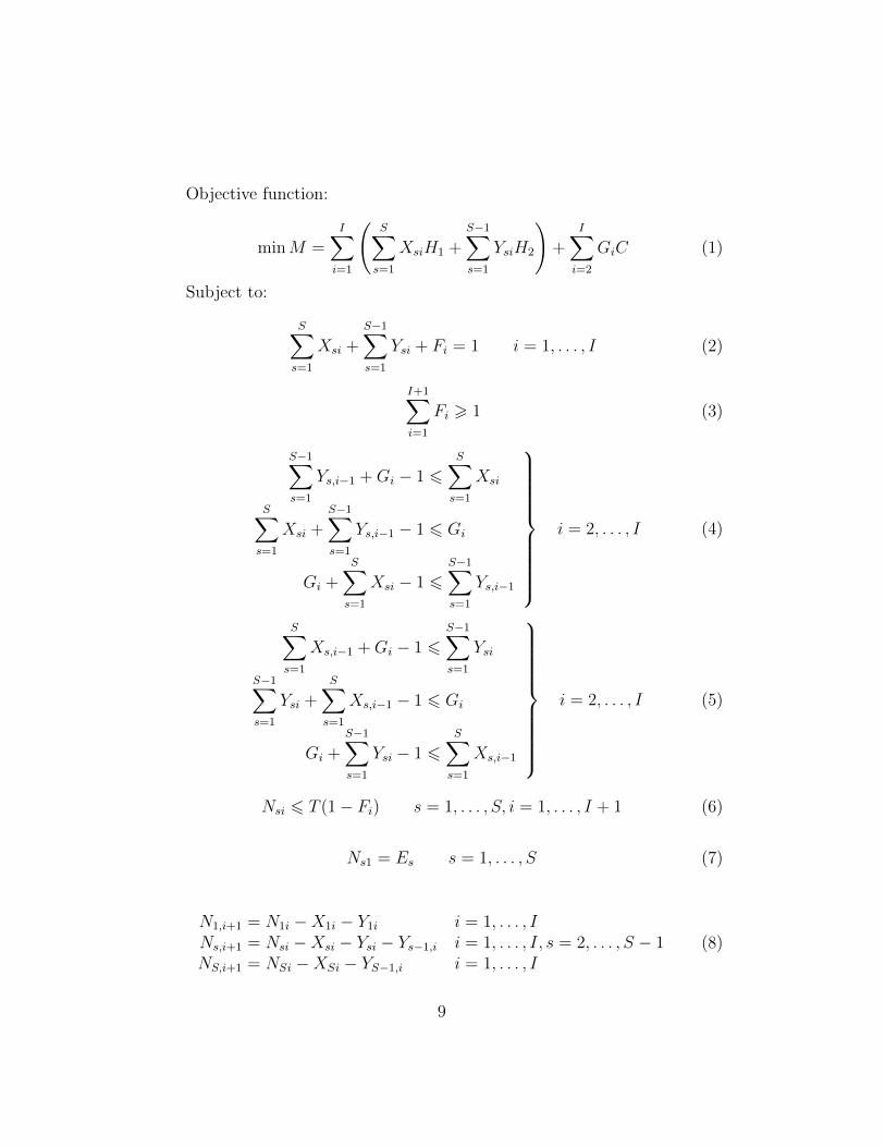
Figure 2 shows an instance of the DSCSP. In this instance, S = 8, T = 3,Es = 3 for all s, and the weights Wst of all containers in the bay are shown inthe upper-left corner of the figure. In addition, we assume that wLimit = 10,H1 = 1.5, H2 = 1.8, and C = 2.1. Note that, even for this small instance,it is not easy to decide which containers should be lifted in single-spreadermode and which containers should be lifted in dual-spreader mode. Figure 2shows a feasible crane lift sequence for this instance. This sequence consistsof five dual-spreader lifts followed by four single-spreader lifts followed by fivedual-spreader lifts. Two changeovers between spreader modes are required,so the total time needed to empty the bay—the makespan—is 10× 1.8 + 4×1.5 + 2 × 2.1 = 28.2 minutes. We later show that this is not the optimalmakespan for this instance.

This paper is organized as follows. Section 2 reviews the relevant litera-ture. In Section 3, we present a mathematical formulation of the DSCSP anda fast method for computing a lower bound on the optimal objective value.In Section 4, we introduce a heuristic method that tries to find good solutions

3

Figure 1. Feasible unloading sequence with makespan 28.2 minutes for a problem instance of size 3x8.

7 5 3 2 6 9 5 4

1 2 4 3 1 2 9 2

6 2 3 6 8 2 7 3

7 5 9

1 2 4 3 1 2 9 2

6 2 3 6 8 2 7 3

7 9

1 2 1 2 9 2

6 2 3 6 8 2 7 3

7 9

1 2 1 2 9 2

6 2 8 2 7 3

9

1 2 1 2 9 2

6 2 8 2 7 3

7 6 9 5 4

1 2 4 3 1 2 9 2

6 2 3 6 8 2 7 3

9

1 2 1 2 9 2

6 2 8 2 7 3

1 2 1 2 2

6 2 8 2 7 3

1 2 1 2 9 2

6 2 8 2 7 3

1 2 1 2

6 2 8 2 7 3

1 2

6 2 8 2 7 3 6 2 8 2 7 3

8 2 7 3 7 3

Double lift = 1.8 min Double lift = 1.8 min

Double lift = 1.8 min

Double lift = 1.8 min

Double lift =

1.8 min

Double lift =

1.8 min

Double lift =

1.8 min

Changeover = 2.1 min Single lift =

1.5 min

Single lift = 1.5 min Single lift = 1.5 min Single lift =

1.5 min

Changeover = 2.1 min Double lift = 1.8 min

FINISHED

2 4

4 3

3 6

7

Double lift = 1.8 min

Double lift = 1.8 min

Figure 2: Feasible crane lift sequence with makespan 28.2 minutes for a problem instanceof size 3× 8 with wLimit = 10.

to instances of the DSCSP within a short time. In Section 5, we describethe experimental setup and discuss the experimental results for two solutionmethods—standard integer programming and the heuristic method—on a setof 120 problem instances. We conclude this paper in Section 6.

2. Literature Review

The authors performed a rigorous search of the academic literature inorder to find published works that previously addressed this topic. In par-

4

ticular, the authors located all works published by one of the “big six”publishers—Elsevier, Springer, INFORMS, Taylor & Francis, Wiley, and Pal-grave Macmillan—that have a title containing any of the phrases “crane,”“spreader,” or “block relocation” in it. For works published by Elsevier andTaylor & Francis, only items falling under the subject categories “decisionsciences” and “economics, finance, business & industry” respectively wereconsidered. Industry journals were also searched. The results of the aboveliterature search yielded several hundred articles, more than half of whichconcern the management of operations at seaport container transhipmentterminals.

Ten articles surveying the literature on seaport container terminal oper-ations were identified, including the works by Vis and De Koster (2003), S-teenken et al. (2004), Stahlbock and Voß (2008), Bierwirth and Meisel (2010),Angeloudis and Bell (2011), Carlo et al. (2014a,b), Carlo et al. (2015), Ghare-hgozli et al. (2015b), and Bierwirth and Meisel (2015). Several of these ar-ticles mention that multi-spreader quay cranes (QCs) are an important newtechnology for container terminal operations. However, no article discusses apublished paper that proposes a method for scheduling multi-spreader QCs.

Scores of papers consider the scheduling of cranes in industries unrelatedto maritime shipping. For example, Dohn and Clausen (2010) solve a cranescheduling problem to optimize slab yard planning in a steel mill. Also, Kunget al. (2014) consider order scheduling of multiple stacker cranes on commonrails in an automated storage and retrieval system. Peterson et al. (2014)propose a method for scheduling multiple factory cranes that operate on acommon track.

Dozens of papers consider yard crane (YC) scheduling problems at sea-port container terminals. For example, Cheung et al. (2002) propose methodsfor deploying YCs among storage blocks in a container terminal. At a moredetailed level, Kim and Kim (1999) develop a math model and exact solu-tion method for routing a single YC. Vis and Carlo (2010) develop a modelfor sequencing the operations of two automated stacking cranes (ASCs) ina container terminal. Li et al. (2012) propose a continuous time model forscheduling multiple YCs that can handle last minute job arrivals. Gharehgo-zli et al. (2015a) develop a math model and heuristic method for schedulingtwo ASCs in a single container storage block. Finally, Wu et al. (2015)present methods for scheduling multiple YCs that prevent YC interferenceand consider safety distance requirements.

Various methods have been developed for scheduling single-spreader QCs

5

at seaport container terminals. For example, Imai et al. (2008) introducea math model of the simultaneous berth and QC allocation problem anddevelop a genetic algorithm to find near-optimal solutions to the problem.Vacca et al. (2013), Turkogulları et al. (2014), Iris et al. (2015), and Li et al.(2015) also consider variations of the simultaneous berth and QC alloca-tion problem. Meisel and Bierwirth (2013) develop methods for solving theintegrated berth allocation, QC allocation, and QC scheduling problem atseaport container terminals. Lee et al. (2011) and Chen et al. (2011) devel-op methods for scheduling QCs at indented berths. Kim and Park (2004)introduce a math model for scheduling QCs at a regular berth and developexact and heuristic methods for solving problem instances. Moccia et al.(2006), Ng and Mak (2006), and Unsal and Oguz (2013) also propose variousQC scheduling methods. Tang et al. (2014) consider a joint QC and truckscheduling problem. Also, Lee et al. (2015) develop an optimal algorithm forthe general QC double-cycling problem.

Discussions of multi-spreader (i.e. tandem-lift) QCs are quite scarce inthe literature. Chao and Lin (2011) present a methodology that trades offthe various features of advanced QCs (including multi-spreader QCs) in or-der to choose a suitable advanced QC for any given container terminal. Xinget al. (2012) and Chen et al. (2014) develop methods for scheduling auto-mated guided vehicles (AGVs) and yard trucks (YTs), respectively, whentandem-lift QCs are used at a container terminal. Choi et al. (2014) use asimulation methodology to develop an operating system that can increase theproductivity of a container terminal where tandem-lift QCs are used. Sev-eral articles in industry journals—including those by McCarthy et al. (2007)and World Cargo News (2007)—contain general discussions of tandem-liftQCs but do not present results related to the scheduling or productivity ofsuch cranes. On the other hand, Song (2011) discusses the productivity oftandem-lift QCs during real-life experiments conducted at Pusan Newportand proposes methods for conducting double cycling operations using suchcranes. Finally, Goussiatiner (2007a,b) generates plausible ship stowage con-figurations in order to compare the productivity of unloading such ships usingsingle-spreader, dual-spreader, and triple-spreader QCs.

Overall, despite the existence of hundreds of published articles on indus-trial cranes, our literature search yielded no published model or method forscheduling multi-spreader cranes. In particular, we did not find any publishedmethod for deciding when a crane should switch between single-spreader anddual-spreader modes. Also, we did not find any method for deciding which

6

containers in a storage bay should be lifted during single-spreader mode anddual-spreader mode. Thus, the problem considered in this article, and themethods for solving it, appear to be unique.

3. Mathematical Model

We now present a math model of the DSCSP. This is the better performingof two models that we developed for this problem. The other model can befound in the supplementary material accompanying this paper.

To facilitate the model development, we first convert the problem instanceinto a “binary array showing legal dual-spreader lifts” (BASLDSL). Figure 3depicts the conversion of the instance in Figure 2 to BASLDSL, where binaryvariables are used to indicate whether a dual-spreader lift could be performedon a pair of adjacent containers in the same tier. Without loss of generality,we use the left side of the pair to denote whether a “legal” dual-spreaderlift can be performed within the given weight limit wLimit. For example, thetop-left ‘0’ in BASLDSL indicates that the first and the second containers(from the left side) in the top tier cannot be dual-spreader lifted because theircombined weight—12—exceeds wLimit = 10. Also, the ‘1’ adjacent to the top-left ‘0’ indicates that the second and the third containers (from the left) inthe top tier can be dual-spreader lifted because their combined weight—8—does not exceed wLimit. In the original problem instance, we number the tiers1, . . . , T from bottom to top and the stacks 1, . . . , S from left to right. InBASLDSL, we use the terms tier (1, . . . , T from bottom to top) and column(1, . . . , S − 1 from left to right) to refer to various locations.

Figure 3. Conversion of problem instance (left) into binary array showing legal dual spreader lifts (right).

Tier 3

Tier 2

Tier 1

Stack: 1 2 3 4 5 6 7 8 Column: 1 2 3 4 5 6 7

7 5 3 2 6 9 5 4

1 2 4 3 1 2 9 2

6 2 3 6 8 2 7 3

0 1 1 1 0 0 1

1 1 1 1 1 0 0

1 1 1 0 1 1 1

Figure 3: Conversion of problem instance (left) into binary array showing legal dual spread-er lifts (right), assuming wLimit = 10.

3.1. Mathematical formulation of the DSCSP

Our mathematical model, model DSCSP, discretizes time into intervals.During each time interval, at most one (single-spreader or dual-spreader) liftmay occur. The duration of an interval is therefore either H1 or H2 minutes

7

depending on the type of operation performed. Between two consecutive in-tervals, at most one spreader changeover may occur (Figure 2).

The indices in model DSCSP are as follows:s Stack, s = 1, 2, . . . , S.t Tier, t = 1, 2, . . . , T .i Time interval, i = 1, 2, . . . , I, I + 1

The input parameters in model DSCSP are as follows:S Number of stacks in the storage bay. S > 2 to avoid triviality.T Number of tiers in the storage bay.I Number of time intervals available (= S × T to be conservative).Es Initial number of containers in stack s, s = 1, . . . , S.C Changeover time between single- and dual-spreader deployment.H1 Handling time per lift using single spreader.H2 Handling time per lift using dual spreader.Lst = 1 if the left side of the dual spreader can be used at stack s,

tier t in the original configuration (s = 1, . . . , S − 1, t = 1, . . . T )(binary). This parameter equals the value of the item in columns, tier t of BASLDSL.

The decision variables in model DSCSP are as follows:Xsi = 1 if a single-spreader lift is performed at the top of stack s

during time interval i (s = 1, . . . , S, i = 1, . . . , I) (binary).Ysi = 1 if a dual-spreader lift is performed in which the left (right)

half of the spreader lifts the container that is on the top of stacks (s + 1) during time interval i (s = 1, . . . , S − 1, i = 1, . . . , I)(binary).

Gi = 1 if a spreader changeover is made between time intervals i− 1and i (i = 2, . . . , I) (binary).

Fi = 1 if we have finished removing all containers from the bay bythe beginning of time interval i (i = 1, . . . , I + 1) (binary).

Nsi Number of containers in stack s at beginning of time interval i(s = 1, . . . , S, i = 1, . . . , I + 1) (integer, > 0).

Rti = 1 if any containers are removed from tier t during time intervali (t = 1, . . . , T , i = 1, . . . , I) (binary).

8

Objective function:

minM =I∑

i=1

(S∑

s=1

XsiH1 +S−1∑s=1

YsiH2

)+

I∑i=2

GiC (1)

Subject to:

S∑s=1

Xsi +S−1∑s=1

Ysi + Fi = 1 i = 1, . . . , I (2)

I+1∑i=1

Fi > 1 (3)

S−1∑s=1

Ys,i−1 + Gi − 1 6S∑

s=1

Xsi

S∑s=1

Xsi +S−1∑s=1

Ys,i−1 − 1 6 Gi

Gi +S∑

s=1

Xsi − 1 6S−1∑s=1

Ys,i−1

i = 2, . . . , I (4)

S∑s=1

Xs,i−1 + Gi − 1 6S−1∑s=1

Ysi

S−1∑s=1

Ysi +S∑

s=1

Xs,i−1 − 1 6 Gi

Gi +S−1∑s=1

Ysi − 1 6S∑

s=1

Xs,i−1

i = 2, . . . , I (5)

Nsi 6 T (1− Fi) s = 1, . . . , S, i = 1, . . . , I + 1 (6)

Ns1 = Es s = 1, . . . , S (7)

N1,i+1 = N1i −X1i − Y1i i = 1, . . . , INs,i+1 = Nsi −Xsi − Ysi − Ys−1,i i = 1, . . . , I, s = 2, . . . , S − 1NS,i+1 = NSi −XSi − YS−1,i i = 1, . . . , I

(8)

9

X1i + Y1i 6 N1i i = 1, . . . , IXsi + Ysi + Ys−1,i 6 Nsi i = 1, . . . , I, s = 2, . . . , S − 1

XSi + YS−1,i 6 NSi i = 1, . . . , I(9)

T∑t=1

Rti = 1 i = 1, . . . , I (10)

−T (1−Xsi) 6T∑t=1

tRti−Nsi 6 T (1−Xsi) i = 1, . . . , I, s = 1, . . . , S (11)

−T (1− Ysi) 6T∑t=1

tRti −Nsi 6 T (1− Ysi)

−T (1− Ysi) 6T∑t=1

tRti −Ns+1,i 6 T (1− Ysi)

i = 1, . . . , I, s = 1, . . . , S−1

(12)

Ysi + Rti − 1 6 Lst s = 1, . . . , S − 1, t = 1, . . . , T, i = 1, . . . , I (13)

The objective function (1) minimizes the makespan, M , which is the sumof the container handling and spreader changeover times. Constraint (2)ensures that at most one lift, either by the single spreader or dual spreader,can be performed during any time interval i; if no lift is made, then the“finished” binary variable Fi should be set to 1. Constraint (3) ensures thatthe process of removing containers from the bay is finished by the end ofthe last time interval. Constraint (4) forces a changeover to happen whenswitching from dual-spreader to single-spreader mode. This constraint hasthree expressions with the following structure: A+B−1 6 C; C+A−1 6 B;and B + C − 1 6 A. These expressions ensure that if any two of the binaryterms A, B, and C equal 1, then the third term equals 1. Term A indicates ifa dual-spreader lift is made during time interval i−1; B indicates if a spreaderchangeover is made between time intervals i − 1 and i; and C indicates ifa single-spreader lift is made during time interval i. Constraint (5) is thesame as (4) except that it considers the switch from single-spreader to dual-spreader mode.

10

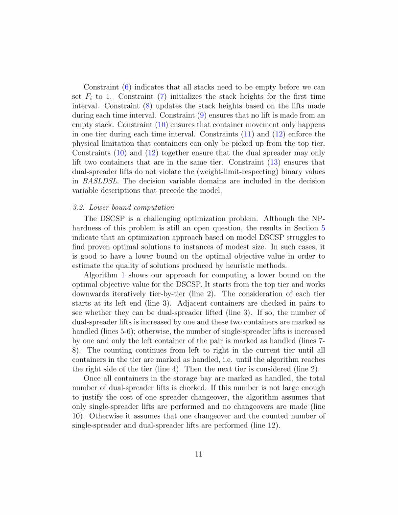
Constraint (6) indicates that all stacks need to be empty before we canset Fi to 1. Constraint (7) initializes the stack heights for the first timeinterval. Constraint (8) updates the stack heights based on the lifts madeduring each time interval. Constraint (9) ensures that no lift is made from anempty stack. Constraint (10) ensures that container movement only happensin one tier during each time interval. Constraints (11) and (12) enforce thephysical limitation that containers can only be picked up from the top tier.Constraints (10) and (12) together ensure that the dual spreader may onlylift two containers that are in the same tier. Constraint (13) ensures thatdual-spreader lifts do not violate the (weight-limit-respecting) binary valuesin BASLDSL. The decision variable domains are included in the decisionvariable descriptions that precede the model.

3.2. Lower bound computation

The DSCSP is a challenging optimization problem. Although the NP-hardness of this problem is still an open question, the results in Section 5indicate that an optimization approach based on model DSCSP struggles tofind proven optimal solutions to instances of modest size. In such cases, itis good to have a lower bound on the optimal objective value in order toestimate the quality of solutions produced by heuristic methods.

Algorithm 1 shows our approach for computing a lower bound on theoptimal objective value for the DSCSP. It starts from the top tier and worksdownwards iteratively tier-by-tier (line 2). The consideration of each tierstarts at its left end (line 3). Adjacent containers are checked in pairs tosee whether they can be dual-spreader lifted (line 3). If so, the number ofdual-spreader lifts is increased by one and these two containers are marked ashandled (lines 5-6); otherwise, the number of single-spreader lifts is increasedby one and only the left container of the pair is marked as handled (lines 7-8). The counting continues from left to right in the current tier until allcontainers in the tier are marked as handled, i.e. until the algorithm reachesthe right side of the tier (line 4). Then the next tier is considered (line 2).

Once all containers in the storage bay are marked as handled, the totalnumber of dual-spreader lifts is checked. If this number is not large enoughto justify the cost of one spreader changeover, the algorithm assumes thatonly single-spreader lifts are performed and no changeovers are made (line10). Otherwise it assumes that one changeover and the counted number ofsingle-spreader and dual-spreader lifts are performed (line 12).

11

Algorithm 1: Lower bound computation

1 Set single-spreader and dual-spreader lift counters Ns = 0, Nd = 0;2 for each tier do3 Starting from the left side of the tier, check whether the next two

containers can be lifted together without violating wLimit;4 while not reaching the right side of the tier do5 if the next two un-handled containers can be dual-spreader

lifted then6 Nd = Nd + 1; mark the next two containers as handled;

7 else8 Ns = Ns + 1; mark the next one container as handled;

9 if NdH2 + C > 2NdH1 then10 LB = H1(Ns + 2Nd);

11 else12 LB = NsH1 + NdH2 + C;

13 Report the lower bound LB;

Theorem 1. Algorithm 1 computes a true lower bound on the optimal ob-jective value for the DSCSP.

Proof 1. Note that a single changeover is only included in the lower boundcomputation if it is profitable; otherwise no changeover is included (lines 9-12). Thus, Algorithm 1 assumes the bare minimum number of changeovers.Consider the value of Nd after the completion of the large “for” loop in Al-gorithm 1 (lines 2-8). We show that this value equals the maximum totalnumber of dual-spreader lifts (i.e. dual lifts) that can be made. This fact,combined with the stipulation H2 < 2H1, will prove the theorem.

Each dual lift is confined to a single tier. Thus, it suffices to show that thegreedy method in Algorithm 1—which accepts all candidate dual lifts as soonas they appear during a left-to-right scan of a given tier—correctly computesthe maximum number of dual lifts that can be made in any given tier.

We prove the correctness of the greedy method by induction. Let D(n)be the maximum number of dual lifts that can be made solely on the right-most n containers in the tier at hand. Clearly, the greedy method correctlycomputes the maximum number of dual lifts that can be made on a set of 1

12

or 2 containers in isolation; thus it correctly computes D(1) and D(2) whenapplied to those sets of containers in isolation.

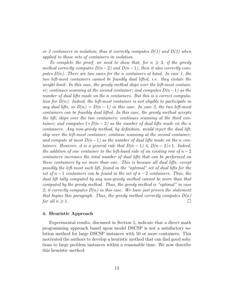
To complete the proof, we need to show that, for n > 3, if the greedymethod correctly computes D(n−2) and D(n−1), then it also correctly com-putes D(n). There are two cases for the n containers at hand. In case 1, thetwo left-most containers cannot be feasibly dual lifted, i.e. they violate theweight limit. In this case, the greedy method skips over the left-most contain-er; continues scanning at the second container; and computes D(n−1) as thenumber of dual lifts made on the n containers. But this is a correct computa-tion for D(n). Indeed, the left-most container is not eligible to participate inany dual lifts, so D(n) = D(n− 1) in this case. In case 2, the two left-mostcontainers can be feasibly dual lifted. In this case, the greedy method acceptsthe lift; skips over the two containers; continues scanning at the third con-tainer; and computes 1+D(n− 2) as the number of dual lifts made on the ncontainers. Any non-greedy method, by definition, would reject the dual lift;skip over the left-most container; continue scanning at the second container;and compute at most D(n−1) as the number of dual lifts made on the n con-tainers. However, it is a general rule that D(n− 1) 6 D(n− 2)+1. Indeed,the addition of one container to the left-hand side of an existing row of n− 2containers increases the total number of dual lifts that can be performed onthese containers by no more than one. This is because all dual lifts, exceptpossibly the left-most such lift, found in the “optimal” set of dual lifts for theset of n− 1 containers can be found in the set of n− 2 containers. Thus, thedual lift tally computed by any non-greedy method cannot be more than thatcomputed by the greedy method. Thus, the greedy method is “optimal” in case2; it correctly computes D(n) in this case. We have just proven the statementthat begins this paragraph. Thus, the greedy method correctly computes D(n)for all n > 1.

4. Heuristic Approach

Experimental results, discussed in Section 5, indicate that a direct mathprogramming approach based upon model DSCSP is not a satisfactory so-lution method for large DSCSP instances with 50 or more containers. Thismotivated the authors to develop a heuristic method that can find good solu-tions to large problem instances within a reasonable time. We now describethis heuristic method.

13

Our overall method consists of a constructive heuristic embedded withina simulated annealing (SA) metaheuristic. The constructive heuristic deter-ministically builds a feasible crane lift sequence based on the values of sixparameters. During each iteration of the SA algorithm, the values of one ormore parameters are changed to new, neighboring values, and a new feasiblecrane lift sequence is generated and evaluated.

We now provide a general description of the constructive heuristic, fol-lowed by a detailed description. Then we discuss the SA algorithm. Theconstructive heuristic is divided into two stages. In stage 1, the type of lift(single-spreader or dual-spreader) for each container is decided. In stage 2, acrane lift sequence—consisting of individual lifts and spreader changeovers—is generated based on the output from stage 1.

Our general approach to stage 1 is to iteratively accept or reject thedual-spreader lift opportunities that are shown in BASLDSL (right side ofFigure 3). Note that the rejection of some dual-lift opportunities is oftennecessary to guarantee feasibility. For example, at least one of the dual-liftopportunities represented by two adjacent ‘ones’ in the same tier in BASLD-SL must be rejected; otherwise, the same container would be involved intwo dual-spreader lifts—one with the container on its left, and one with thecontainer on its right. Importantly, the dual-lift opportunities are not con-sidered individually, but rather in batches of contiguous dual-lifts that arealigned vertically (i.e. in batches of consecutive ‘ones’ in the same column inBASLDSL). The consideration of such a batch often, but not always, resultsin all dual-lifts in the batch being accepted. To maintain feasibility, everyacceptance is followed by the immediate rejection of all dual lift opportuni-ties in the columns immediately to the right and left of the accepted batch’scolumn in BASLDSL. The output from stage 1 is a modified, or fixed, versionof BASLDSL in which (1) the respective values are less than or equal to thosein the initial BASLDSL and (2) there are no adjacent ‘ones’ in the same tier.

In stage 2, we use the fixed BASLDSL to label each container in the baywith a “S” (“D”) if it will be single-spreader (dual-spreader) lifted. Thenwe construct a feasible crane lift sequence by iteratively removing containersfrom the tops of the stacks in the bay if they match the current spreaderbeing deployed. When no more lifts can be made using the current spreader,the spreader is changed. Lifting then continues using the new spreader. Thisprocess continues until no more containers remain in the bay. The makespanof the crane lift sequence is then computed.

We now describe the constructive heuristic in greater detail. Table 1 lists

14

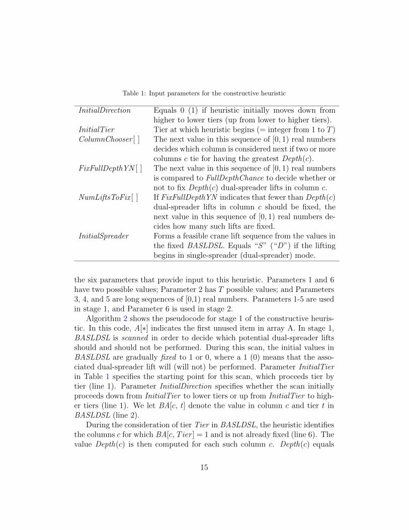
Table 1: Input parameters for the constructive heuristic

InitialDirection Equals 0 (1) if heuristic initially moves down fromhigher to lower tiers (up from lower to higher tiers).

InitialTier Tier at which heuristic begins (= integer from 1 to T )ColumnChooser [ ] The next value in this sequence of [0, 1) real numbers

decides which column is considered next if two or morecolumns c tie for having the greatest Depth(c).

FixFullDepthYN [ ] The next value in this sequence of [0, 1) real numbersis compared to FullDepthChance to decide whether ornot to fix Depth(c) dual-spreader lifts in column c.

NumLiftsToFix [ ] If FixFullDepthYN indicates that fewer than Depth(c)dual-spreader lifts in column c should be fixed, thenext value in this sequence of [0, 1) real numbers de-cides how many such lifts are fixed.

InitialSpreader Forms a feasible crane lift sequence from the values inthe fixed BASLDSL. Equals “S” (“D”) if the liftingbegins in single-spreader (dual-spreader) mode.

the six parameters that provide input to this heuristic. Parameters 1 and 6have two possible values; Parameter 2 has T possible values; and Parameters3, 4, and 5 are long sequences of [0,1) real numbers. Parameters 1-5 are usedin stage 1, and Parameter 6 is used in stage 2.

Algorithm 2 shows the pseudocode for stage 1 of the constructive heuris-tic. In this code, A[∗] indicates the first unused item in array A. In stage 1,BASLDSL is scanned in order to decide which potential dual-spreader liftsshould and should not be performed. During this scan, the initial values inBASLDSL are gradually fixed to 1 or 0, where a 1 (0) means that the asso-ciated dual-spreader lift will (will not) be performed. Parameter InitialTierin Table 1 specifies the starting point for this scan, which proceeds tier bytier (line 1). Parameter InitialDirection specifies whether the scan initiallyproceeds down from InitialTier to lower tiers or up from InitialTier to high-er tiers (line 1). We let BA[c, t] denote the value in column c and tier t inBASLDSL (line 2).

During the consideration of tier Tier in BASLDSL, the heuristic identifiesthe columns c for which BA[c, Tier] = 1 and is not already fixed (line 6). Thevalue Depth(c) is then computed for each such column c. Depth(c) equals

15

Algorithm 2: Stage 1 of the constructive heuristic

1 Set Phase = 1, Dir = InitialDirection, and Tier = InitialTier ;2 Let BA[c, t] denote the value in column c and tier t in BASLDSL;3 Set Fixed [c, t] = no for all (c, t) in BASLDSL;4 while Tier > 1 (6 T ) when Dir = 0 (1) do5 Set Fixed [c, Tier ] = yes for all c such that BA[c, Tier ] = 0;6 while Fixed [c, Tier ] = no for any c from 1 to S − 1 do7 For all c ∈ 1, . . . , S − 1 for which Fixed [c, Tier ] = no, let

Depth(c) be the number of consecutive ‘ones’ that appear incolumn c in BASLDSL beginning with tier Tier and movingdown (up) if Dir = 0 (1). Let CGD be the column c with thegreatest Depth(c). Break ties using ColumnChooser [* ];

8 if FixFullDepthYN [* ] 6 FullDepthChance then9 DualLiftsFixed = Depth(CGD);

10 else11 DualLiftsFixed = floor(Depth(CGD)×NumLiftsToFix [* ]);

12 if DualLiftsFixed = 0 then13 Set BA[CGD, Tier ] = 0 and Fixed [CGD, Tier ] = yes;

14 else15 Fix DualLiftsFixed ‘ones’ in column CGD in direction Dir

in BASLDSL. In other words, set BA[CGD, t ] = 1 andFixed [CGD, t ] = yes for all t from Tier toTier -DualLiftsFixed+1 if Dir = 0 or from Tier toTier+DualLiftsFixed -1 if Dir = 1;

16 Fix DualLiftsFixed ‘zeros’ in the columns adjacent tocolumn CGD in direction Dir in BASLDSL;

17 Decrease (increase) Tier by 1 if Dir = 0 (1);18 if Phase = 1 and Dir = 0 (1) and Tier = 0 (T + 1) and InitialTier

< T (> 1) then19 Set Phase = 2, Dir = 1 (0), and Tier = InitialTier ;20 Set Fixed [c, InitialTier ] = no for all c from 1 to S − 1;

21 Report the BASLDSL with fixed values;

16

Algorithm 3: The constructive heuristic

1 Convert the problem instance into BASLDSL (see Figure 3);2 Call Algorithm 2 to fix the values in BASLDSL;3 Convert BASLDSL into ContainerArray, an S × T array that shows

the type of container occupying each cell in the storage bay. “S”(“D”) indicates a container that will be single-spreader(dual-spreader) lifted. “n” indicates that no container is present. LetCA[s, t] denote the value in stack s and tier t in ContainerArray ;

4 Set CurrSpreader = InitialSpreader ;5 while there is at least one “S” or “D” in ContainerArray do6 for t = T to 1 (decrease t by 1 each time) do7 for s = 1 to S (increase s by 1 each time) do8 if CA[s, t] = CurrSpreader = “S” and (CA[s, t+1] = “n”

or does not exist) then9 Add a single-spreader lift to the end of the crane lift

sequence and let CA[s, t] = “n”;

10 if CA[s, t] = CurrSpreader = “D” then11 if CA[s, t+1] = CA[s+1, t+1] = “n” or neither value

exists then12 Add a dual-spreader lift to the end of the crane lift

sequence and let CA[s, t] = CA[s+1, t] = “n”;

13 Increase s by 1

14 Change CurrSpreader from “S” to “D” or vice versa;

15 if the crane lift sequence has short, unprofitable subsequences ofdual-spreader lifts that are not worth the changeover cost then

16 Convert the unprofitable dual-spreader lifts into single-spreaderlifts in the crane lift sequence;

17 Report the final crane lift sequence and its makespan M ;

the number of consecutive ‘ones’ in column c that begin at tier Tier and pro-ceed upwards or downwards depending on the current scanning direction Dir(line 7). The dual-spreader opportunities in the column c with the greatestDepth(c) are the first candidates for acceptance. When two or more columnsc tie for having the greatest Depth(c), the next [0,1) real number in array

17

ColumnChooser [ ] breaks the tie and selects the “column with the greatestdepth” (i.e. CGD) (line 7). In particular, if L columns are tied, then the nthsuch column is selected if and only if (n− 1)/L 6 ColumnChooser [*] < n/L.The next [0,1) real number in array FixFullDepthYN [ ] is then comparedto global parameter FullDepthChance (line 8) to decide if all Depth(CGD)dual-spreader lift opportunities in column CGD are accepted (line 9) or not(lines 10-11). If not, the next [0,1) real number in array NumLiftsToFix [ ] in-dicates what fraction of the dual-spreader lift opportunities are accepted, i.e.to what depth the ‘ones’ in the column are fixed. In particular, the numberof ‘ones’ that are fixed equals floor(Depth(CGD)×NumLiftsToFix [* ]) (line11). If this equals 0 (line 12), the single dual-lift opportunity in columnCGD, tier Tier is rejected and the corresponding cell in BASLDSL is fixedto 0 (line 13). Otherwise, one or more dual-lift opportunities in column CGDare accepted (i.e. a sub-column of ‘ones’ in BASLDSL is fixed) (line 15), andthe values in all cells on either side of this sub-column are fixed to 0 (line 16).The latter step ensures that two adjacent ‘ones’ in the same tier in BASLD-SL are never both fixed. This concludes the handling of column CGD in thecurrent tier. Other columns c are then considered one-at-a-time according tothe ranking of their Depth(c) values, and the above process repeats until allvalues in the current tier in BASLDSL have been fixed to 1 or 0 (lines 6-16).

The procedure then continues to the next tier in the current scanningdirection Dir (line 17). Eventually all tiers in direction Dir will be scanned.At that point, the second phase of the scanning commences: the procedurejumps back to tier InitialTier, un-fixes all values in that tier, and beginsscanning in the direction opposite from InitialDirection (lines 19-20). Thissecond phase is undertaken if and only if InitialTier is a middle tier (line18). After completion of the second phase, all tiers in BASLDSL have beenscanned and all cells in BASLDSL have been fixed (line 21).

The overall constructive heuristic is shown in Algorithm 3. This heuristicfirst calls Algorithm 2 to fix the values in BASLDSL (line 2). It then convertsthe fixed BASLDSL into a ContainerArray, an S×T array that shows whichcontainers in the storage bay will be single-spreader (“S”) and dual-spreader(“D”) lifted. A detailed crane lift sequence that starts using spreader Initial-Spreader is then constructed in a straightforward manner using the valuesin ContainerArray (lines 4-14). If the end (middle) of the sequence containsshort, unprofitable subsequences of dual-spreader lifts that are not worth thecost of one (two) spreader changeover(s), the unprofitable dual-spreader liftsare converted into single-spreader lifts (lines 15-16). Then the makespan of

18

Figure 4. Illustration #1 of the constructive heuristic. The most recent activity in BASLDSL is highlighted.

Fixed values in BASLDSL are displayed in bold.

0 1 1 1 0 1 0

1 1 1 1 1 0 0

1 1 1 0 1 1 1

0 13 13 12 0 11 0

1 1 1 1 1 0 0

1 1 1 0 1 1 1

7 3 5 2 6 5 9 4

1 4 2 3 1 9 2 2

6 3 2 6 8 7 2 3

S D D D D D S D

S D D D D S S S

S D D S D D D D

S S

S S S S

S S D D D D

D D D D

Six dual lifts = 6*1.8 min

Changeover = 2.1 min

Eight single lifts = 8*1.5 min Changeover = 2.1 min

FINISHED

Two dual lifts = 2*1.8 min

Heuristic Input Parameters:

InitialDirection = 0 InitialTier = 3 ColumnChooser = [0, 0, 0, 0, … FixFullDepthYN = [0, 0, 0, 0, … NumLiftsToFix = [0, 0, 0, 0, … InitialSpreader = D

Global Parameters:

FullDepthChance = 0.5

ContainerArray:

Makespan = 30.6 min

All subsequences of dual-spreader lifts (the six lifts at the start, the two lifts at the end) are worth the

setup cost of the dual spreader

Original problem instance Initial BASLDSL Note: Superscripts show Depth(c) for each column c. Phase = 1 Dir = 0 Tier = 3 ColumnChooser[1] = 0 CGD = 2 FixFullDepthYN[1] = 0 DualLiftsFixed = 3 CGD = 4 FixFullDepthYN[2] = 0 DualLiftsFixed = 2

CGD = 7 FixFullDepthYN[3] = 0 DualLiftsFixed = 1 Tier = 2

Tier = 1 ColumnChooser[2] = 0 CGD = 5 FixFullDepthYN[4] = 0 DualLiftsFixed = 1 CGD = 7 FixFullDepthYN[5] = 0 DualLiftsFixed = 1 BASLDSL with

fixed values

0 0 1 12

0 11

0

0 0 1 1 1 0 0

0 0 1 0 1 1 1

0 0 1 1

0 11

0

0 0 1 1 0 0 0

0 0 1 0 1 1 1

0 0 1 1

0 1

0 0 0 1 1 0 0 0

0 0 1 0 1 1 1

0 0 1 1

0 1

0

0 0 1 1 0 0 0 0 0 1 0 1 1 1

0 0 1 1

0 1

0

0 0 1 1 0 0 0 0 0 1 0 11 11 11

0 0 1 1

0 1

0

0 0 1 1 0 0 0 0 0 1 0 1 11

0

0 0 1 1

0 1

0

0 0 1 1 0 0 0 0 0 1 0 1 1

0

0 0 1 1

0 1

0

0 0 1 1 0 0 0 0 0 1 0 1 1

0

InitialSpreader = D

Figure 4: Illustration #1 of the constructive heuristic. The most recent activity in BASLD-SL is highlighted. Fixed values in BASLDSL are displayed in bold.

19

Figure 5. Illustration #2 of the constructive heuristic. The most recent activity in BASLDSL is highlighted.

Fixed values in BASLDSL are displayed in bold.

0 1 1 1 0 1 0

1 1 1 1 1 0 0

1 1 1 0 1 1 1

0 1 1 1 0 1 0

11 12 12 12 11 0 0 1 1 1 0 1 1 1

7 3 5 2 6 5 9 4

1 4 2 3 1 9 2 2

6 3 2 6 8 7 2 3

S D D D D S S S

D D D D D S D S

D D D D D D D D

Six single lifts = 6*1.5 min Changeover = 2.1 min Nine dual lifts = 9*1.8 min

FINISHED

Heuristic Input Parameters:

InitialDirection = 1 InitialTier = 2 ColumnChooser = [.4, .8, .9, .7, .5, .2, … FixFullDepthYN = [.7, 0, 0, .9, 0, 0, 0, 0, 0, 0 NumLiftsToFix = [.6, .9, … InitialSpreader = S

Global Parameters:

FullDepthChance = 0.5

ContainerArray:

Makespan = 27.3 min

All subsequences of dual-spreader lifts are worth the setup cost of the

dual spreader

Original problem instance Initial BASLDSL Note: Superscripts show Depth(c) for each column c. Phase = 1 Dir = 1 Tier = 2 ColumnChooser[1] = .4 CGD = 3 FixFullDepthYN[1] = .7 NumLiftsToFix[1] = .6 DualLiftsFixed = floor(2*.6) = 1 ColumnChooser[2] = .8 CGD = 5 FixFullDepthYN[2] = 0 DualLiftsFixed = 1 CGD = 1 FixFullDepthYN[3] = 0 DualLiftsFixed = 1 Tier = 3

ColumnChooser[3] = .9 CGD = 7 FixFullDepthYN[4] = .9 NumLiftsToFix [2] = .9 DualLiftsFixed = floor(1*.9) = 0 ColumnChooser[4] = .7 CGD = 4 FixFullDepthYN[5] = 0 DualLiftsFixed = 1 CGD = 2 FixFullDepthYN[6] = 0 DualLiftsFixed = 1 Tier = 4 Phase = 2 Dir = 0 Tier = 2

0 1 1 1 0 1 0

11

1

0

0

11

0 0

1 1 1 0 1 1 1

0 1 1 1 0 1 0

11

1

0

0

1

0 0 1 1 1 0 1 1 1

0 1 1 1 0 1 0

1

1

0

0

1

0 0 1 1 1 0 1 1 1

0 11 11 11 0 11 0 1

1

0

0

1

0 0 1 1 1 0 1 1 1

0 11

11

11

0 0 0

1

1

0

0

1

0 0 1 1 1 0 1 1 1

0 0

11

1

0 0 0 1

1

0

0

1

0 0 1 1 1 0 1 1 1

0 0

1

1

0 0 0 1

1

0

0

1

0 0 1 1 1 0 1 1 1

0 0

1

1

0 0 0 12

12

0

0

12

0 0

1 1 1 0 1 1 1

0 0

1

1

0 0 0 12

1

0

0

12

0 0

1 1 0 0 1 1 1

0 0

1

1

0 0 0

1

1

0

0

12

0 0

1 1 0 0 1 1 1

0 0

1

1

0 0 0

1

1

0

0

1

0 0 1 1 0 0 1 1 0

0 0

1

1

0 0 0

1

1

0

0

1

0 0 1 1 0 0 1 1 0

ClmChose[5] = .5 CGD = 3 FFDpthYN[7] = 0 DualLftFixed = 2 ClmChose[6] = .2 CGD = 1 FFDpthYN[8] = 0 DualLftFixed = 2

CGD = 5 FFDpthYN[9] = 0 DualLftFixed = 2 Tier = 1 CGD = 7 FFDpthYN[10] = 0 DualLftFixed = 1

InitialSpreader = S

Figure 5: Illustration #2 of the constructive heuristic. The most recent activity in BASLD-SL is highlighted. Fixed values in BASLDSL are displayed in bold.

20

Figure 6. Overall logic of the simulated annealing metaheuristic.

Set the temperature CurrTemp = InitialTemp

Set BestOV = 999,999,999.

Let CurrParam be the following set of parameters: 1. InitialDirection = 0 2. InitialTier = T 3. ColumnChooser[ ] = [0, 0, 0, … , 0] 4. FixFullDepthYN[ ] = [0, 0, 0, … , 0] 5. NumLiftsToFix[ ] = [0, 0, 0, … , 0] 6. InitialSpreader = S

Convert CurrParam into a crane lift sequence, CurrSeq, and compute its objective value, CurrOV, using the constructive heuristic (i.e. Alg. 3).

No

Yes

Convert NghborParam into a crane lift sequence, NghborSeq, and compute its objective value, NghborOV, using the constructive heuristic (i.e. Alg. 3).

Yes

Is CurrOV < BestOV ?

No

Set BestOV = CurrOV Set BestParam = CurrParam Set BestSeq = CurrSeq

Has the time limit been reached ?

Have all four possibilities for parameters (1, 6)—namely (0, S), (0, D), (1, S), (1, D)—been explored for the current set of values of parameters (2, 3, 4, 5) ? In other words, have all four possibilities for CurrParam in the current sub-neighborhood been explored ?

No Yes

Large Nbhd Move: Set NghborParam = CurrParam except that (i) one parameter (2, 3, 4, 5) is set to a new, random value/array with probability (p2, p3, p4, p5) and (ii) parameters (1, 6) are set to new, random values.

Small Nbhd Move: Set NghborParam = CurrParam except that parameters (1, 6) are set to a new, random ordered pair that has not been explored during the stay in this sub-neighborhood.

Is NghborOV - CurrOV = Δ ≤ 0 ?

Yes No

Is rand[0,1) ≤ e-Δ/CurrTemp ? Set CurrOV = NghborOV Set CurrParam = NghborParam Set CurrSeq = NghborSeq

Yes

No

Set CurrTemp = CurrTemp * TempFactor

Display BestOV, BestParam, BestSeq.

Figure 6: Overall logic of the simulated annealing metaheuristic.

21

the resulting crane lift sequence is computed (line 17).Figures 4 and 5 show how the constructive heuristic generates two dif-

ferent crane lift sequences for the problem instance shown in Figure 3 basedon two sets of input parameters. In each figure, the original problem in-stance and its conversion into the initial, tentative BASLDSL are shown inthe upper-left. The values of the six input parameters are shown in theupper-right. The left side of each figure shows how Algorithm 2 graduallyfixes the values in BASLDSL using the first five parameters. Note that onlythe first several values in arrays ColumnChooser [ ], FixFullDepthYN [ ], andNumLiftsToFix [ ] are utilized; the other values are not used. The conver-sion of the fixed BASLDSL into ContainerArray ; the generation of a detailedcrane lift sequence; and the makespan computation are shown in the bottom-right. Notice that the fixed BASLDSL, ContainerArray, and makespan arequite different in the two figures. Indeed, the constructive heuristic is ableto generate vastly different crane lift sequences when the input parametersare changed. It turns out that the makespan shown in Figure 5 is optimal.

Figure 6 shows how the constructive heuristic is embedded within a sim-ulated annealing (SA) framework. The SA procedure begins by initializingthe six input parameters, collectively referred to as CurrParam, and convert-ing them into a feasible crane lift sequence CurrSeq and makespan CurrOVusing the constructive heuristic. In each SA iteration, CurrParam is usedto generate a new set of parameter values NghborParam; the constructiveheuristic converts NghborParam into a feasible crane lift sequence; and thelaws of simulated annealing decide if NghborParam replaces CurrParam.

Two kinds of neighborhood moves–small moves and large moves—are uti-lized. In a small move, a new, random combination of values for parameters1 and 6—InitialDirection and InitialSpreader—is considered and the otherparameters remain unchanged. In a large move, a new, random value forparameter (2, 3, 4, 5) is considered with probability (p2, p3, p4, p5) anda new, random combination of values for parameters 1 and 6 is considered(p2+p3+p4+p5 = 1). A small move is made whenever it can produce a newset of parameter values that has not yet been explored. Otherwise, a largemove is initiated. When a predefined time limit is reached, the SA procedureterminates and the best crane lift sequence that was found is displayed.

22

5. Experimental Setup, Results and Discussion

The heuristic method from Section 4 and model DSCSP from Section 3were coded into MS Visual C++ 2010 Professional. IBM ILOG ConcertTechnology was used to define model DSCSP within C++ and call the MILPsolver IBM ILOG CPLEX 12.5 to solve instances defined in text files. Toavoid running out of memory, the CPLEX “node file storage parameter” isset to 3. That is, the information for every unexplored node in the branch-and-cut tree is stored on the hard disk and compressed. Otherwise, defaultCPLEX settings are used. All results are obtained using a desktop computerwith the Windows 7 Enterprise 64-bit operating system, an Intel Core i7-4770processor with eight 3.4 GHz cores, and 16 GB of RAM.

We consider a total of 120 problem instances—30 instances for each of theproblem sizes 3×8, 5×10, 10×23, and 50×50. A problem of size T×S has Sstacks, T tiers, and T containers in stack s for all s at time 0. In all instances,we assume that the container weights Wst take integer values from 1 to 9.We also assume that wLimit = 10, H1 = 1.5, H2 = 1.8, and C = 2.1. Amongthe 30 instances for each problem size, (10, 10, 10) instances have (light,medium, heavy) container weights. In the medium instances, the weight ofeach container follows a discrete uniform distribution over the values 1, 2,3, 4, 5, 6, 7, 8, 9. In the light instances, the weight of each container hasa 15%, 15%, 15%, 15%, 20%, 5%, 5%, 5%, 5% chance of taking the value1, 2, 3, 4, 5, 6, 7, 8, 9. In the heavy instances, the weight of each containerhas a 5%, 5%, 5%, 5%, 20%, 15%, 15%, 15%, 15% chance of taking thevalue 1, 2, 3, 4, 5, 6, 7, 8, 9. Text files defining all problem instances canbe found in the supplementary material accompanying this paper.

Table 2 shows the settings used in the heuristic algorithm for each of thefour problem sizes. Preliminary experiments were performed to determinethese settings. The results of these preliminary experiments, not shown here,indicated that performance was most consistent when the neighbor probabil-ities (p2, p3, p4, p5) equal (.25, .25, .25, .25) (Figure 6). We also found thatperformance improves with a higher FullDepthChance (line 8 of Algorithm 2,middle of Table 1) as the problem size increases. We hypothesize that this isbecause instances with more tiers can have larger batches of dual lift oppor-tunities that are aligned vertically (i.e. longer strings of consecutive ‘ones’in the same column in the initial BASLDSL). As the size of such a batch in-creases, it may be increasingly important to accept all dual lift opportunitiesin the batch to prevent “disrupting” the batch with a single rejected dual

23

Table 2: Parameter settings for the heuristic method

Problem Size 3× 8 5× 10 10× 23 50× 50

Computational time limit (seconds) 10 60 600 600FullDepthChance 0.5 0.7 0.8 0.99Neighbor probabilities (p2, p3, p4, p5) all set to (.25, .25, .25, .25)InitialTemp 10,000 100,000 10,000,000 100,000TempFactor 0.9999 0.99999 0.999999 0.99999

lift opportunity in its middle. Such a disruption may add two unnecessarychangeovers—to and from the single spreader—to the crane lift sequence.

Note that more computation time is allocated for attacking larger prob-lems. Given this time limit, parameters InitialTemp and TempFactor are setso the SA procedure consists of three phases of roughly equal duration—(i) aninitial exploration phase when almost any neighboring solution is accepted;(ii) a middle phase when the algorithm gradually transitions from being veryaccepting of neighbors to being very picky; and (iii) a final phase when virtu-ally no inferior neighboring solutions are accepted. The increase (decrease)in parameters InitialTemp and TempFactor when going from problem size3× 8 to 10× 23 (10× 23 to 50× 50) follows from the fact that the allottedcomputation time grows at a faster (slower) rate than the problem size forthese instances.

Table 3 shows the results for the first set of experiments that consider the30 small problem instances of size 3×8. Each individual instance is specifiedby a code “TxSZnn” where T is the number of tiers; S is the number of stack-s; “Z” takes the values (L, M, H) according to the container weight scenarios(light, medium, heavy); and “nn” denotes the instance number from 1 to 10.Each instance is considered in three ways—(A) using standard integer pro-gramming (IP) with no time limit (“CPLEX Alone”); (B) using the heuristicmethod with a 10 sec time limit; and (C) using IP with no time limit whereboth the lower bound and the best solution found by the heuristic are passedto the solver at the outset (“CPLEX+LB+UB”). The heuristic method gen-erates an average of eleven million neighboring solutions within the 10 sectime limit. The best objective value (i.e. makespan) found by methods A,B, and C are shown in columns MCP, MH , and MCP+B respectively. ColumnMH0 shows the makespan of the initial feasible solution used in the heuristicmethod, and column LB shows the lower bound.

The results show that all three methods solve all instances to optimali-

24

ty. Indeed, method A solves all instances to optimality within ten minutes;method B finds these optimal solutions within ten seconds; and method Csolves all instances to optimality within three minutes. Importantly, thebest solutions found by the heuristic (all of which happen to be optimal)are usually within 5% of the lower bound. Also, the objective value of thebest heuristic solution (30.3) is about 7% better on average than that of theinitial heuristic solution (32.6). Not surprisingly, the optimal values for thelight instances are typically less than those for the medium instances. Thesame holds for the medium instances compared to the heavy instances.

Table 4 shows the results for the second set of experiments that considerthe 30 medium-sized instances of size 5×10. Here, each instance is consideredin three ways—(A) using IP with a one hour time limit (“CPLEX Alone”);(B) using the heuristic method with a 60 sec time limit; and (C) using IP witha one hour time limit where the lower bound and best solution found by theheuristic are passed to the solver at the outset (“CPLEX+LB+UB”). Theheuristic method generates an average of 31 million neighboring solutionswithin the 60 sec time limit. Column “Opt?” indicates if the associatedsolution is proven to be optimal or not.

The results for methods A and B show that the heuristic method performsbetter than IP. Indeed, in every instance, the best solution found by theheuristic in one minute is at least as good as the best solution found byCPLEX in an hour. Also, the average objective value of the best heuristicsolution (62.6) is about 1.4% better than that for CPLEX (63.5). Note thatthe best solutions found by the heuristic (only two of which are known to beoptimal) are about 6% higher on average than the lower bound. Also, theresults for method C show that CPLEX is unable, in an hour, to improveupon the best heuristic solution provided to it at the outset for any instance.These observations give us confidence that the heuristic method is findingnear-optimal or optimal solutions to these instances. Finally, we observe thatthe objective value of the best heuristic solution (62.6) is about 5% lower onaverage than that of the initial heuristic solution (65.7). Overall, the aboveresults indicate that our IP framework is not a suitable solution method forinstances with 50 or more containers. Thus, IP is not considered in thefollowing experiments that consider larger problem instances.

Table 5 shows the results for the 60 largest problem instances—30 largeinstances of size 10×23 and 30 very large instances of size 50×50. The resultsfor the large (very large) instances are on the left (right). For each instance,we show the lower bound; the objective value of the best solution found by

25

Table 3: Experimental results for instances of size 3× 8. Optimal solutions are found byall three approaches.

CPLEX Alone Heuristic (10 seconds) CPLEX+LB+UB

Instance MCP Time (s) MH MH0

MH0−MH

MHMCP+B Time (s) LB MH−LB

MH

3x8L01 27.3 17 27.3 29.4 7.69% 27.3 15 26.1 4.40%3x8L02 26.1 12 26.1 31.8 21.84% 26.1 0 26.1 0.00%3x8L03 26.1 6 26.1 27.3 4.60% 26.1 1 26.1 0.00%3x8L04 29.4 211 29.4 31.8 8.16% 29.4 112 27.3 7.14%3x8L05 21.6 1 21.6 28.2 30.56% 21.6 1 21.6 0.00%3x8L06 27.3 80 27.3 33.9 24.18% 27.3 71 26.1 4.40%3x8L07 24.9 4 24.9 28.2 13.25% 24.9 0 24.9 0.00%3x8L08 30.6 573 30.6 31.8 3.92% 30.6 157 28.5 6.86%3x8L09 26.1 7 26.1 30.6 17.24% 26.1 0 26.1 0.00%3x8L10 28.2 424 28.2 31.5 11.70% 28.2 75 26.1 7.45%Average 26.8 133.5 26.8 30.5 14.31% 26.8 43.2 25.9 3.02%3x8M01 30.6 8 30.6 31.8 3.92% 30.6 42 28.5 6.86%3x8M02 30.9 37 30.9 30.9 0.00% 30.9 25 29.7 3.88%3x8M03 27.3 29 27.3 31.8 16.48% 27.3 53 26.1 4.40%3x8M04 34.2 76 34.2 35.7 4.39% 34.2 55 32.1 6.14%3x8M05 30.9 109 30.9 33.0 6.80% 30.9 108 28.5 7.77%3x8M06 27.3 7 27.3 33.0 20.88% 27.3 0 27.3 0.00%3x8M07 30.9 56 30.9 33.0 6.80% 30.9 63 29.7 3.88%3x8M08 32.1 17 32.1 33.0 2.80% 32.1 24 30.9 3.74%3x8M09 34.2 14 34.2 34.2 0.00% 34.2 31 32.1 6.14%3x8M10 28.5 6 28.5 30.6 7.37% 28.5 33 27.3 4.21%Average 30.7 35.9 30.7 32.7 6.94% 30.7 43.4 29.2 4.70%3x8H01 35.7 6 35.7 36.0 0.84% 35.7 19 34.5 3.36%3x8H02 32.1 27 32.1 34.2 6.54% 32.1 40 30.9 3.74%3x8H03 35.7 9 35.7 36.0 0.84% 35.7 12 34.5 3.36%3x8H04 29.7 10 29.7 31.8 7.07% 29.7 0 29.7 0.00%3x8H05 33.3 8 33.3 35.4 6.31% 33.3 1 33.3 0.00%3x8H06 34.5 7 34.5 35.4 2.61% 34.5 19 33.3 3.48%3x8H07 32.1 24 32.1 32.1 0.00% 32.1 38 30.9 3.74%3x8H08 32.1 8 32.1 35.4 10.28% 32.1 16 30.9 3.74%3x8H09 34.2 22 34.2 34.2 0.00% 34.2 25 32.1 6.14%3x8H10 36.0 1 36.0 36.0 0.00% 36.0 1 36.0 0.00%Average 33.5 12.2 33.5 34.7 3.45% 33.5 17.1 32.6 2.76%Ovrl Avg. 30.3 60.5 30.3 32.6 8.24% 30.3 34.6 29.2 3.49%

26

Table 4: Experimental results for instances of size 5× 10.

CPLEX Alone Heuristic (60 seconds) CPLEX+LB+UB

Instance MCP Time (s) Opt? MH MH0

MH0−MH

MHMCP+B Time (s) Opt? LB MH−LB

MH

5x10L01 62.1 3861 ? 61.2 63.0 2.94% 61.2 3605 ? 56.7 7.35%5x10L02 55.2 3915 ? 55.2 63.6 15.22% 55.2 3610 ? 53.1 3.80%5x10L03 57.3 4001 ? 56.4 61.2 8.51% 56.4 3608 ? 53.1 5.85%5x10L04 56.1 3726 ? 55.2 58.8 6.52% 55.2 3607 ? 51.9 5.98%5x10L05 50.7 3673 ? 50.7 60.0 18.34% 50.7 3603 ? 49.5 2.37%5x10L06 66.0 3665 ? 63.3 67.8 7.11% 63.3 3605 ? 57.9 8.53%5x10L07 56.1 3850 ? 56.1 61.2 9.09% 56.1 3604 ? 51.9 7.49%5x10L08 56.4 4114 ? 56.4 57.6 2.13% 56.4 3605 ? 53.1 5.85%5x10L09 51.6 3604 ? 51.6 58.8 13.95% 51.6 3779 ? 49.5 4.07%5x10L10 51.6 3600 ? 51.6 59.4 15.12% 51.6 3663 ? 49.5 4.07%Avg. 56.3 3800.9 55.8 61.1 9.89% 55.8 3628.9 52.6 5.54%5x10M01 67.8 3602 ? 64.8 66.6 2.78% 64.8 3605 ? 60.3 6.94%5x10M02 63.9 3766 ? 62.4 66.0 5.77% 62.4 3604 ? 57.9 7.21%5x10M03 63.9 3611 ? 63.6 66.0 3.77% 63.6 3606 ? 60.3 5.19%5x10M04 64.8 3769 ? 64.8 67.2 3.70% 64.8 3606 ? 61.5 5.09%5x10M05 66.0 3658 ? 64.8 64.8 0.00% 64.8 3607 ? 61.5 5.09%5x10M06 62.1 3669 ? 57.6 59.7 3.65% 57.6 3603 ? 54.3 5.73%5x10M07 60.6 3625 ? 59.7 63.0 5.53% 59.7 3604 ? 54.3 9.05%5x10M08 68.1 3726 ? 66.9 69.9 4.48% 66.9 3607 ? 61.5 8.07%5x10M09 64.2 3652 ? 62.1 63.3 1.93% 62.1 3606 ? 57.9 6.76%5x10M10 57.3 3602 ? 55.5 61.8 11.35% 55.5 3604 ? 51.9 6.49%Avg. 63.9 3668 62.2 64.8 4.30% 62.2 3605.2 58.1 6.56%5x10H01 74.4 223 yes 74.4 74.4 0.00% 74.4 114 yes 72.3 2.82%5x10H02 69.9 3641 ? 69.3 70.5 1.73% 69.3 3608 ? 65.1 6.06%5x10H03 70.2 3606 ? 66.9 68.1 1.79% 66.9 3603 ? 62.7 6.28%5x10H04 69.3 3608 ? 66.9 67.8 1.35% 66.9 3604 ? 61.5 8.07%5x10H05 75.0 41 yes 75.0 75.0 0.00% 75.0 104 yes 73.5 2.00%5x10H06 72.9 3690 ? 72.9 73.2 0.41% 72.9 3607 ? 66.3 9.05%5x10H07 69.6 3602 ? 69.6 72.0 3.45% 69.6 3608 ? 66.3 4.74%5x10H08 62.4 3669 ? 62.4 65.7 5.29% 62.4 3623 ? 59.1 5.29%5x10H09 69.6 3609 ? 69.6 72.0 3.45% 69.6 3606 ? 66.3 4.74%5x10H10 70.8 3616 ? 70.8 71.7 1.27% 70.8 3606 ? 67.5 4.66%Avg. 70.4 2930.5 69.8 71.0 1.87% 69.8 2908.3 66.1 5.37%Ovrl Avg. 63.5 3466.5 62.6 65.7 5.35% 62.6 3380.8 58.9 5.82%

27

the heuristic method within a 600 sec time limit; and the objective value ofthe initial heuristic solution. The heuristic method generates an average of39 (1.9) million neighboring solutions within the 600 sec time limit for theinstances of size 10× 23 (50× 50).

The results show that the heuristic is finding near-optimal solutions tothese instances. Indeed, the average objective value of the best heuristicsolution for the instances of size 10 × 23 and 50 × 50—275.2 and 2936.8respectively—is about 4% higher than the average lower bound—263.8 and2828.9 respectively—for these instances. Also, note that the quality of theheuristic solution improves as containers get heavier; on average, the makespanof the best heuristic solution is roughly 5%, 4%, and 3% above the lowerbound for the light, medium, and heavy instances respectively. This maybe due to the fact that there are fewer opportunities for using the dualspreader—and therefore fewer choices—when containers are heavier.

28

Table 5: Experimental results for instances of size 10× 23 (left) and 50× 50 (right) withthe heuristic running for 600 seconds.

Instance LB MH MH0

MH0−MH

MH

MH−LBMH

Instance LB MH MH0

MH0−MH

MH

MH−LBMH

10x23L01 228.3 237.9 249.6 4.92% 4.04% 50x50L01 2496.9 2628.6 2676.6 1.83% 5.01%10x23L02 225.9 234.6 242.4 3.32% 3.71% 50x50L02 2471.7 2605.5 2659.8 2.08% 5.14%10x23L03 231.9 241.8 254.7 5.33% 4.09% 50x50L03 2500.5 2625.9 2661.9 1.37% 4.78%10x23L04 228.3 239.4 253.5 5.89% 4.64% 50x50L04 2490.9 2621.1 2667.3 1.76% 4.97%10x23L05 231.9 243.9 258.9 6.15% 4.92% 50x50L05 2492.1 2645.7 2689.2 1.64% 5.81%10x23L06 230.7 240.6 246.3 2.37% 4.11% 50x50L06 2514.9 2644.8 2692.5 1.80% 4.91%10x23L07 235.5 247.5 260.4 5.21% 4.85% 50x50L07 2505.3 2621.4 2658.0 1.40% 4.43%10x23L08 229.5 243.0 249.6 2.72% 5.56% 50x50L08 2472.9 2593.2 2632.8 1.53% 4.64%10x23L09 237.9 248.7 266.7 7.24% 4.34% 50x50L09 2494.5 2616.0 2668.5 2.01% 4.64%10x23L10 237.9 247.5 259.5 4.85% 3.88% 50x50L10 2489.7 2632.8 2684.4 1.96% 5.44%Average 231.8 242.5 254.2 4.80% 4.41% Average 2492.9 2623.5 2669.1 1.74% 4.98%10x23M01 264.3 278.1 281.4 1.19% 4.96% 50x50M01 2792.1 2902.5 2925.0 0.78% 3.80%10x23M02 259.5 273.6 280.8 2.63% 5.15% 50x50M02 2789.7 2899.2 2919.6 0.70% 3.78%10x23M03 263.1 274.8 283.2 3.06% 4.26% 50x50M03 2801.7 2902.5 2929.8 0.94% 3.47%10x23M04 260.7 272.4 279.6 2.64% 4.30% 50x50M04 2834.1 2944.8 2970.0 0.86% 3.76%10x23M05 269.1 279.9 284.4 1.61% 3.86% 50x50M05 2818.5 2915.7 2940.6 0.85% 3.33%10x23M06 265.5 279.3 285.6 2.26% 4.94% 50x50M06 2810.1 2918.4 2942.1 0.81% 3.71%10x23M07 264.3 274.8 277.2 0.87% 3.82% 50x50M07 2793.3 2915.7 2931.0 0.52% 4.20%10x23M08 255.9 264.3 272.4 3.06% 3.18% 50x50M08 2780.1 2912.4 2931.9 0.67% 4.54%10x23M09 261.9 273.6 279.6 2.19% 4.28% 50x50M09 2819.7 2940.9 2958.0 0.58% 4.12%10x23M10 261.9 273.6 274.8 0.44% 4.28% 50x50M10 2772.9 2889.6 2902.2 0.44% 4.04%Average 262.6 274.4 279.9 2.00% 4.30% Average 2801.2 2914.2 2935.0 0.72% 3.88%10x23H01 293.1 304.8 309.6 1.57% 3.84% 50x50H01 3208.5 3294.0 3300.3 0.19% 2.60%10x23H02 294.3 306.9 308.1 0.39% 4.11% 50x50H02 3188.1 3268.2 3287.4 0.59% 2.45%10x23H03 299.1 309.6 315.3 1.84% 3.39% 50x50H03 3196.5 3272.7 3279.6 0.21% 2.33%10x23H04 296.7 309.3 311.4 0.68% 4.07% 50x50H04 3167.7 3258.6 3273.0 0.44% 2.79%10x23H05 300.3 310.8 314.4 1.16% 3.38% 50x50H05 3186.9 3264.6 3277.8 0.40% 2.38%10x23H06 295.5 308.1 308.1 0.00% 4.09% 50x50H06 3216.9 3290.4 3302.4 0.36% 2.23%10x23H07 294.3 306.9 307.2 0.10% 4.11% 50x50H07 3204.9 3281.1 3289.2 0.25% 2.32%10x23H08 299.1 310.8 315.6 1.54% 3.76% 50x50H08 3201.3 3286.5 3297.6 0.34% 2.59%10x23H09 297.9 308.4 308.4 0.00% 3.40% 50x50H09 3189.3 3265.5 3277.8 0.38% 2.33%10x23H10 299.1 309.6 315.3 1.84% 3.39% 50x50H10 3165.3 3246.3 3256.2 0.30% 2.50%Average 296.9 308.5 311.3 0.91% 3.75% Average 3192.5 3272.8 3284.1 0.35% 2.45%Ovrl Avg. 263.8 275.2 281.8 2.57% 4.16% Ovrl Avg. 2828.9 2936.8 2962.8 0.93% 3.77%

29

6. Conclusion

In this paper, we proposed a new crane scheduling problem inspired by thedual-spreader quay crane, an emerging technology that has been deployed atsome container ports around the world. The efficient operation of such cranesmay allow containerships to be unloaded more quickly. We formulated theproblem as a mixed-integer linear program, developed a tight lower boundon the optimal value, and devised a heuristic approach for handling largeproblem instances. The heuristic approach begins with an excellent initialfeasible solution that effectively utilizes the problem structure. A simulatedannealing framework was used to improve upon the initial feasible solution.

Numerical experiments indicate that the heuristic approach finds thesame optimal solutions as CPLEX for small-sized instances. For medium-sized instances, the heuristic always outperforms CPLEX. The comparisonbetween the optimal value and lower bound for small-sized instances suggeststhat the lower bound is tight, providing a good guide for solution quality.Overall, the heuristic approach produces crane schedules whose makespans,on average, are within 6% of the lower bound for each of the four problemsizes considered.

Although we solely consider the unloading of a storage bay, our approachcan apply to the loading of a storage bay. Indeed, reversing the sequenceof operations—single-spreader lifts, dual-spreader lifts, and changeovers—creates a schedule for loading a storage bay in the same amount of time inwhich it is unloaded.

Future work might proceed in several directions. First, the NP-hardnessof this problem could be established. Second, other types of problem in-stances could be considered. In the instances we considered, parametersH1, H2, and C were multiples of 0.3, so the objective value was restrictedto being a multiple of 0.3. This might have hindered the search for bettersolutions within our optimization and heuristic approaches. Instances withmore realistic positions of heavy and light containers—e.g. heavy contain-ers at the bottom—could also be considered. Third, better optimization orheuristic approaches that use completely different search strategies could bedeveloped. Finally, different variations of this problem—that include ad-ditional real-world constraints and/or consider the distance moved by thespreader—might be considered.

30

Acknowledgements

No ghost writers or ghost computer programmers were involved in theproduction of this manuscript. The authors thank three anonymous reviewersfor several helpful comments that strengthened this paper.

References

Angeloudis, P., Bell, M. G., 2011. A review of container terminal simulationmodels. Maritime Policy & Management 38 (5), 523–540.

Bierwirth, C., Meisel, F., 2010. A survey of berth allocation and quay cranescheduling problems in container terminals. European Journal of Opera-tional Research 202 (3), 615–627.

Bierwirth, C., Meisel, F., 2015. A follow-up survey of berth allocation andquay crane scheduling problems in container terminals. European Journalof Operational Research 244 (3), 675–689.

Carlo, H. J., Vis, I. F., Roodbergen, K. J., 2014a. Storage yard operations incontainer terminals: Literature overview, trends, and research directions.European Journal of Operational Research 235 (2), 412–430.

Carlo, H. J., Vis, I. F., Roodbergen, K. J., 2014b. Transport operations incontainer terminals: Literature overview, trends, research directions andclassification scheme. European Journal of Operational Research 236 (1),1–13.

Carlo, H. J., Vis, I. F., Roodbergen, K. J., 2015. Seaside operations incontainer terminals: Literature overview, trends, and research directions.Flexible Services and Manufacturing Journal 27 (2-3), 224–262.

Chao, S.-L., Lin, Y.-J., 2011. Evaluating advanced quay cranes in containerterminals. Transportation Research Part E: Logistics and TransportationReview 47 (4), 432–445.

Chen, J. H., Lee, D.-H., Cao, J. X., 2011. Heuristics for quay crane schedulingat indented berth. Transportation Research Part E: Logistics and Trans-portation Review 47 (6), 1005–1020.

31

Chen, L. H., Cao, J. X., Zhao, Q. Y., 2014. Tandem lift quay cranes and yardtrucks scheduling problem at container terminals. In: Applied Mechanicsand Materials. Vol. 505. Trans Tech Publ, pp. 927–930.

Cheung, R. K., Li, C.-L., Lin, W., 2002. Interblock crane deployment incontainer terminals. Transportation Science 36 (1), 79–93.

Choi, S.-H., Im, H., Lee, C., 2014. Development of an operating systemfor optimization of the container terminal by using the tandem-lift quaycrane. In: Park, J. J., Stojmenovic, I., Choi, M., Xhafa, F. (Eds.), FutureInformation Technology. Springer, Berlin, pp. 399–404.

Dohn, A., Clausen, J., 2010. Optimising the slab yard planning and cranescheduling problem using a two-stage heuristic. International Journal ofProduction Research 48 (15), 4585–4608.

Gharehgozli, A. H., Laporte, G., Yu, Y., de Koster, R., 2015a. Schedulingtwin yard cranes in a container block. Transportation Science 49 (3), 686–705.

Gharehgozli, A. H., Roy, D., de Koster, R., 2015b. Sea container terminals:New technologies and or models. Maritime Economics & Logistics.

Goussiatiner, A., 2007a. In pursuit of productivity. Container ManagementAugust.

Goussiatiner, A., 2007b. In pursuit of productivity 2. Container ManagementSeptember.

Imai, A., Chen, H. C., Nishimura, E., Papadimitriou, S., 2008. The simulta-neous berth and quay crane allocation problem. Transportation ResearchPart E: Logistics and Transportation Review 44 (5), 900–920.

Iris, C., Pacino, D., Ropke, S., Larsen, A., 2015. Integrated berth allocationand quay crane assignment problem: Set partitioning models and com-putational results. Transportation Research Part E: Logistics and Trans-portation Review 81, 75–97.

Kim, K. H., Kim, K. Y., 1999. An optimal routing algorithm for a transfercrane in port container terminals. Transportation Science 33 (1), 17–33.

32

Kim, K. H., Park, Y.-M., 2004. A crane scheduling method for port containerterminals. European Journal of Operational Research 156 (3), 752–768.

Kung, Y., Kobayashi, Y., Higashi, T., Sugi, M., Ota, J., 2014. Order schedul-ing of multiple stacker cranes on common rails in an automated stor-age/retrieval system. International Journal of Production Research 52 (4),1171–1187.

Lee, C.-Y., Liu, M., Chu, C., 2015. Optimal algorithm for the general quaycrane double-cycling problem. Transportation Science 49 (4), 957–967.

Lee, D.-H., Chen, J. H., Cao, J. X., 2011. Quay crane scheduling for anindented berth. Engineering Optimization 43 (9), 985–998.

Li, F., Sheu, J.-B., Gao, Z.-Y., 2015. Solving the continuous berth allocationand specific quay crane assignment problems with quay crane coveragerange. Transportation Science 49 (4), 968–989.

Li, W., Goh, M., Wu, Y., Petering, M. E. H., de Souza, R., Wu, Y. C.,2012. A continuous time model for multiple yard crane scheduling withlast minute job arrivals. International Journal of Production Economics136 (2), 332–343.

McCarthy, P. W., Jordan, M. A., Wright, L., 2007. Dual-hoist, tandem 40crane considerations. Port Technology International 34, 111–113.

Meisel, F., Bierwirth, C., 2013. A framework for integrated berth allocationand crane operations planning in seaport container terminals. Transporta-tion Science 47 (2), 131–147.

Moccia, L., Cordeau, J.-F., Gaudioso, M., Laporte, G., 2006. A branch-and-cut algorithm for the quay crane scheduling problem in a containerterminal. Naval Research Logistics (NRL) 53 (1), 45–59.

Ng, W., Mak, K., 2006. Quay crane scheduling in container terminals. Engi-neering Optimization 38 (6), 723–737.

Peterson, B., Harjunkoski, I., Hoda, S., Hooker, J. N., 2014. Scheduling mul-tiple factory cranes on a common track. Computers & Operations Research48, 102–112.

33

Song, J.-H., 2011. Tandem operation and double cycling in container termi-nals. Port Technology International 51, 73–79.

Stahlbock, R., Voß, S., 2008. Operations research at container terminals: aliterature update. OR Spectrum 30 (1), 1–52.

Steenken, D., Voß, S., Stahlbock, R., 2004. Container terminal operationand operations research-a classification and literature review. OR spectrum26 (1), 3–49.

Tang, L., Zhao, J., Liu, J., 2014. Modeling and solution of the joint quaycrane and truck scheduling problem. European Journal of Operational Re-search 236 (3), 978–990.

Turkogulları, Y. B., Taskın, Z. C., Aras, N., Altınel, I. K., 2014. Optimalberth allocation and time-invariant quay crane assignment in containerterminals. European Journal of Operational Research 235 (1), 88–101.

Unsal, O., Oguz, C., 2013. Constraint programming approach to quay cranescheduling problem. Transportation Research Part E: Logistics and Trans-portation Review 59, 108–122.

Vacca, I., Salani, M., Bierlaire, M., 2013. An exact algorithm for the integrat-ed planning of berth allocation and quay crane assignment. TransportationScience 47 (2), 148–161.

Vis, I. F., Carlo, H. J., 2010. Sequencing two cooperating automated stackingcranes in a container terminal. Transportation Science 44 (2), 169–182.

Vis, I. F., De Koster, R., 2003. Transshipment of containers at a containerterminal: An overview. European journal of operational research 147 (1),1–16.

World Cargo News, 2007. Make mine a double – or even a triple.

Wu, Y., Li, W.-K., Petering, M., Goh, M., de Souza, R., 2015. Schedulingmultiple yard cranes with crane interference and safety distance require-ment. Transportation Science 49 (4), 990–1005.

Xing, Y., Yin, K., Quadrifoglio, L., Wang, B., 2012. Dispatch problem of au-tomated guided vehicles for serving tandem lift quay crane. TransportationResearch Record (2273), 79–86.

34