Sequence Evolution and the Mechanism of Protein Folding

Sequence Evolution and the Mechanism of Protein Folding

Angel R. Ortiz and Jeffrey SkolnickDepartment of Molecular Biology, TPC-5, The Scripps Research Institute, La Jolla, California 92037 USA

ABSTRACT The impact on protein evolution of the physical laws that govern folding remains obscure. Here, by analyzingin silico-evolved sequences subjected to evolutionary pressure for fast folding, it is shown that: First, a subset of residues inthe thermodynamic folding nucleus is mainly responsible for modulating the protein folding rate. Second and most important,the protein topology itself is of paramount importance in determining the location of these residues in the structure. Furtherstabilization of the interactions in this nucleus leads to fast folding sequences. Third, these nucleation points restrict thesequence space available to the protein during evolution. Correlated mutations between positions around these hot spotsarise in a statistically significant manner, and most involve contacting residues. When a similar analysis is carried out on realproteins, qualitatively similar results are obtained.

INTRODUCTION

Prediction of protein structure from sequence is widelyrecognized as one of the most important unsolved problemsin molecular biology, and it has become more pressing withthe current blossoming of genome sequencing projects(Koonin, 1997, Koonin, et al., 1998). Many of the currentapproaches to protein structure prediction rely on relatingsequence patterns to structural ones, particularly with theavailability of multiple sequence alignments (MSAs) formany sequences of interest. But finding sequence–structurerelationships requires discrimination from functional oreven adventitious patterns in current databases that may nothave unique correspondence with structure. Signatures re-lated to protein topology are the needles to be found in thehaystack of alignments. Also, because topology is the out-come of the folding mechanism, relationships among se-quence space, the folding process, and final topology needto be established. In summary, a better understanding of theconstraints imposed during protein evolution by the physi-cal laws that govern folding is required.

The acquisition of such understanding is a formidabletask. To make the problem tractable, simplified lattice mod-els of protein-like chains have been developed by a numberof authors (Shakhnovich, 1996). In particular, Shakhnovichand coworkers (Mirny, et al., 1998) recently generated adatabase of fast and slow folding models of homologousproteins (48-mers on a cubic lattice, see Methods and Fig. 2)by using evolution-like pressure for fast folding. Here, afteranalyzing these fast and slow folding model proteins andafter doing similar calculations on real proteins, we reportthat structurally significant patterns can appear in MSAs ofevolutionary related sequences. We observe that correlatedmutations tend to occur between contacting residues, andthat they seem to arise as a consequence of the evolutionary

constraint to fold sufficiently fast to the global energyminimum. They tend to be located closer than expected bychance to the residues forming the protein folding nucleus.These correlations could also be topology dependent, be-cause we show that the topology itself determines whichresidues form part of the folding nucleus.

METHODS

Database of model proteins

A database formed by in silico evolutionary related sequences of slow andfast folding model proteins was generously provided to us by Dr. E.Shakhnovich (personal communication). This database consists of;1000sequences of model proteins created by folding randomly mutated se-quences of 48-mers on a cubic lattice subjected to evolutionary pressure forfast folding (Mirny, et al., 1998). The conformation to which all thesesequences fold is shown in Fig. 2.

Multivariate analysis of the sequences ofmodel proteins

Factor Analysis (Reyment and Joreskog, 1996) (FA) has been used toderive statistical models that explain the differences between fast and slowfolding sequences. FA tries to describe the covariance relationships in adata matrix in terms of underlying, but unobservable, random quantitiesknown as factors. The factors are new variables, or directions in space,built from linear combinations of the original variables in such a way thatthey account approximately for the same amount of information of theoriginal variables in the data matrix. This is achieved by grouping variablesby their correlations. Mathematically speaking, FA seeks finding an un-derlying orthogonal factor model of an originalX matrix of the form

X 5 LF 1 E. (1)

In Eq. 1, X is a matrix derived from the MSA and havingn rows,corresponding ton positions in the alignment; andm columns, correspond-ing to m sequences being aligned. On the right-hand side,L is the loadingsmatrix andF the scores matrix, whereasE is the residual (noise) matrix.Each elementl ip of the matrixL can be considered as the square root of theweight (or importance) of the variablei on factor p. That is, it is thecontribution of variable (i.e., the position)i on building the new directionp. In contrast each component scorefpj from the matrixF can be consideredthe projection of the object (i.e., the sequence)j on factorp, or, in otherwords, the coordinate of objectj in the new direction given by factorp.

Received for publication 18 June 1999 and in final form 24 February 2000.

Address reprint requests to Dr. Angel Ramirez Ortiz, Assistant Professor,Department of Physiology and Biophysics, Mount Sinai School of Medi-cine, One Gustave Levy Pl., Box 1218, New York, NY 10029.

© 2000 by the Biophysical Society

0006-3495/00/10/1787/13 $2.00

1787Biophysical Journal Volume 79 October 2000 1787–1799

The existence of this model implies a special covariance structure forX.It can be shown that, under the assumption thatF andE are orthogonal andindependent, this covariance structureXX * can be expressed as

XX * 5 ~LF 1 E!~LF 1 E!9, (2)

XX * 5 S5 LL * 1 U. (3)

HereX* is the transpose ofX, andU 5 EE* is the covariance of the noisematrix, which, under the factor model conditions, contains the specific (notinterrelated and therefore not explained by the model) variances of theobjects, assumed to be small:U > 0. The solution to the factor model canthen be obtained by diagonalization of the covariance structureXX *. Thisis known as theprincipal component solutionto the factor model (Johnsonand Wichern, 1992). By using the Eckart–Young theorem (Reyment andJoreskog, 1996),S can be expressed as

S5 PLP* 5 PL1/2L1/2*P* 5 ~PL1/2!~PL1/2!9. (4)

Thus, by comparing Eqs. 3 and 4, we can obtain the loadings as

L 5 PL1/2. (5)

Equation 5 indicates that the loadings are no more than the scaledeigenvectors of the symmetric matrixS. If principal components analysisis used as a solution of the factor model using Eq. 5 to obtain the loadings,then it is customary to generate the scores by an ordinary (unweighted)least squares procedure (Johnson and Wichern, 1992). Starting from Eq. 1,and assumingE > 0, then

L *X 5 L *LF , (6)

F 5 ~L *L !21L *X. (7)

Using Eqs. 3, 4, and 5, Eq. 7 can be expressed as

F 5 ~L1/2*P*PL1/2!21~PL1/2!9X, (8)

F 5 L21/2P*X. (9)

Thus, the factor model can be solved using Eqs. 5 and 9 after diago-nalizing the covariance structureXX *. After a lower dimensionality spaceof p factors explaining most of the variance of the originalX-matrix isfound, in FA, one proceeds to rotate the factors until a simpler structure isachieved (Reyment and Joreskog, 1996). This is done to obtain a betterinterpretation of the factors, and it is possible because Eq. 3 is insensitiveto any orthogonal transformation of the loadings,

XX * 5 S5 LL * 1 U 5 LTT *L * 1 U

where TT * 5 I . (10)

The ideal rotation matrixT to apply toL would generate a new loadingsmatrix so that each variable has the simplest interpretation in the newspace. This would be achieved by having in the rotated loadings matrixL*as many zero elements as possible. In this way, a variable would notdepend on all common factors but only on a small part of them. This isequivalent to maximizing the total variance of the loading elements in thep selected factors. A popular way to obtain such a multidimensionalrotation is by means of thevarimax rotation, where an iterative pairwisebidimensional rotation method due to Kaiser (1958) is used to find anorthogonal optimal rotation matrixG that maximizes a measure of thevariances of the loadings known as the Harman function,f:

f 5 Oj51

n Oi51

p

~dij2 2 d# j!

2 5 Oj51

n Oi51

p

dij4 2 pO

j51

n

d# j2, (11)

where

dij 5l ijhi

(12)

and

d# j 5 p21 Oi51

p

dij2 . (13)

Here,l ij is the ij element of the loadings matrixL, hi is the square root ofthe communality of the variablei (that is, the variance explained by thefactor model),n equals the total number of variables, andp is the dimen-sionality of the loadings matrix. The rotation matrixG that maximizes Eq.11 is used to obtain the rotated loadings by using the transformation,

L* 5 LG . (14)

The FA of the MSA was carried out using the correlation matrix, insteadof the covariance matrix, as follows: The correlation matrixR was derivedby first defining an exchange matrix at each sequence position in thealignment where each pair of elements in the position is scored by amodified version of the McLachlan matrix [optimized to maximize thecontact prediction ability, (Ortiz and Skolnick, in preparation)], and thencomputing a Pearson-type correlation coefficient between exchange matri-ces at any two positions. Thus, the elementr ij of R is obtained,

r ij 51

N2 Okl

~sikl 2 ^si&!~sjkl 2 ^sj&!

sisj. (15)

Wherei andj are two different positions in the MSA, and the indicesk andl run from 1 to theN of sequences in the family. The parametersikl (sjkl )is the comparison score of the amino acids of sequencesk andl at positioni (j) of the alignment. Average values over all aligned sequences atpositionsi andj are given by si& and ^sj&, whereassi andsj correspond totheir standard deviation. Afterwards, the PCA solution to the R-mode FAmodel was obtained by diagonalizatingR. The firstp 5 3 dimensions werescaled and subjected to a varimax rotation to obtain the loadings matrix.We have seen by trial and error that three factors contain enough varianceto explore the main differences in the alignments without being anchoredin the rotation by the less significant factors so that they provide optimalseparation of residues and sequences, and, therefore, the clearest interpre-tation of the FA model. From the rotated loadings, the scores werecomputed by ordinary least squares.

Prediction of contacts and correlatedmutation analysis

The procedure is based on computing theR matrix from the MSA, asdefined above, followed by the sequential application of FA (Reyment andJoreskog, 1996) to eliminate phylogenetic relationships and partial corre-lation (Johnson and Wichern, 1992) to eliminate indirect effects of inter-vening or indirect variables. Typically, and for proteins up to about 100residues, between 5 and 10 contacts are selected. A more detailed accountof this methodology for contact prediction can be found in Ortiz, et al.(1999), and an extensive evaluation for real proteins will be given in asubsequent publication. For the proteins studied in this paper, the MSAswere obtained from the HSSP database (Sander and Schneider, 1991) forthose proteins present in the protein databank (Bernstein, et al., 1977). Asfor the CASP3 proteins, a detailed account of the creation of the corre-sponding MSAs is presented in a separate publication (Ortiz, et al., 1999).

1788 Ortiz and Skolnick

Biophysical Journal 79(4) 1787–1799

Identification of kinetically hot residuesby the GNM

The basic idea behind the Gaussian Network Model (GNM) (Bahar, etal., 1997) is to consider the folded protein as a three-dimensional (3D)elastic network where residues undergo Gaussian fluctuations around theirmean positions resulting from harmonic potentials between residues incontact. The Kirchhoff matrix of contactsG describes the dynamic char-acteristics of this network. This matrix is the counterpart of the stiffnessmatrix used in the analysis of elastic bodies, and itsij element is definedas

Gij 5 5H~rc 2 r ij! if i Þ j

2 Oi(Þj)

N

Gij if i 5 j . (16)

WhereN is the total number of residues;rc is the contacting distance of tworesidues measured in the Ca positions (a value ofrc 5 7 was used in thiswork); r ij is the distance between the Ca positions of the residuesi and j;andH(x) is the Heaviside step function, given asH(x) 5 21 if x . 0 andH(x) 5 0 if x # 0. The inverse matrixG21 yields correlations between thethermal fluctuations per residue. Thus, the cross-correlation in the motionof pairs of residues is associated with thekth vibrational mode by theequation,

^DRiDRj&k 5 ~3kBT/g!lk21uku9kij . (17)

From the above equation, the mean square fluctuation of residuei vibratingin a given subset of modes can be obtained from

^~DRi!2&k12k2 5 ~kBT/g! O

k5k1

k5k2

lk21@uk#i

2Y Ok5k1

k5k2

lk21 . (18)

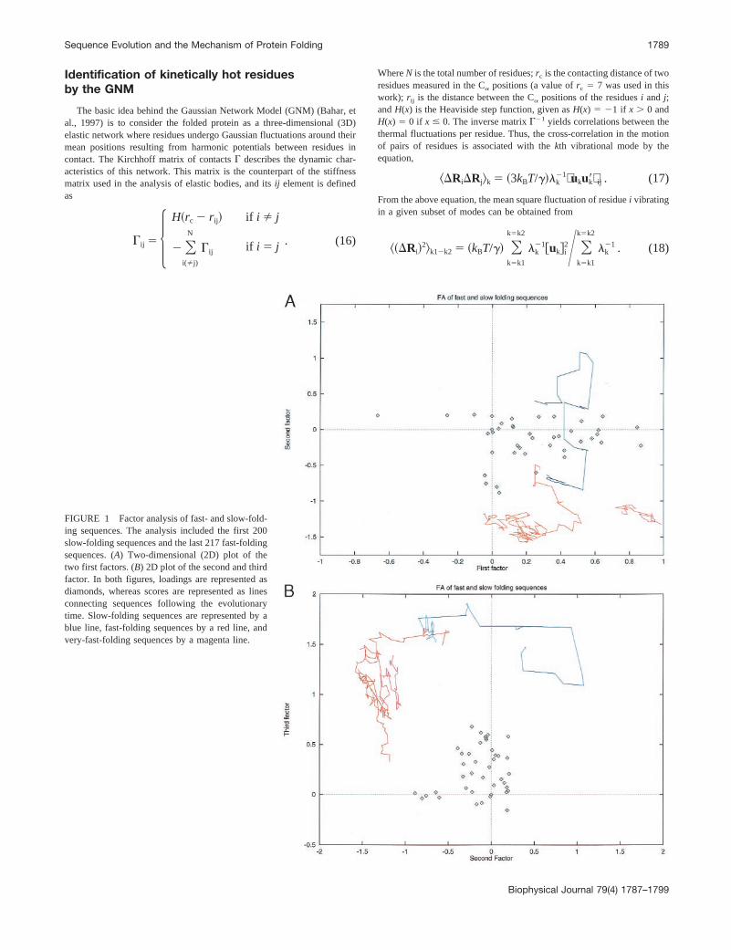
FIGURE 1 Factor analysis of fast- and slow-fold-ing sequences. The analysis included the first 200slow-folding sequences and the last 217 fast-foldingsequences. (A) Two-dimensional (2D) plot of thetwo first factors. (B) 2D plot of the second and thirdfactor. In both figures, loadings are represented asdiamonds, whereas scores are represented as linesconnecting sequences following the evolutionarytime. Slow-folding sequences are represented by ablue line, fast-folding sequences by a red line, andvery-fast-folding sequences by a magenta line.

Sequence Evolution and the Mechanism of Protein Folding 1789


Following Demirel et al. (1998), we study the mean square fluctuationsinduced by the modesN 2 4 # k , N. As in their study, we consider“kinetically hot residues” to be those residues in these modes having anaverage mean square fluctuation above 6N21.

Interaction energy analysis

Let us denote each one of theN positions of the lattice model byi. Inthe global minimum conformation, each position has a given contactcoordination numbernci, with each contactk contributing an energyES(ncik) for a given sequence. The homology averaged energy of eachposition in the global minimum is given by

Ei 51

N seqz nciOS

Ok

EiS~ncik!. (19)

This value can be averaged over a window 2w 1 1 to consider the meanhomology-averaged energy of the different fragments in the structure,

E# i 51

2w 1 1 Oj5i2w

j5i1w

Ej . (20)

The excess energy (normalized in its structural context) of each residueis then a measure related to thelocal frustration of that residue in itsstructural context,

Fi 5 ~Ei 2 E# i! 2 ^Ei 2 E# i& (21)

whereas the average stability of the fragment in which the residue isimmersed is given by

Si 5 E# i 2 ^E# i&. (22)

Nonparametric regression

The nonparametric regression functionm(X) of a response variableY inmeasuring a set of variablesX is defined as the conditional mean ofY onX, i.e., m(X) 5 E(YuX). Thus, for a given sample of design variables{ X i} i51

n , the associated response variables {Y i} i51n are of the form:

Yi 5 m~X i! 1 «i with i 5 1, . . . ,n, (23)

where {«i} i51n are independent errors. Within a given sample, thenonpara-

metric estimatem of the functionm has the general form

m~X! 5 Oi

wi~X!yi with Oi

wi~X!1. (24)

Several nonparametric estimates have been proposed in the statisticalliterature. In this work, we considered the shifted Nadaraya–Watson(SNW) estimate (Mammen and Marron, 1997), which appears stable whendata are sparse (Hardle and Marron, 1995). The SNW estimate is definedas

mSNW~x! 5Oi51

n Kh~xi 2 j21~x!!yiOi51n Kh~xi 2 j21~x!!

, (25)

with

j~x! 5Oi51

n Kh~xi 2 x!)xiOi51n Kh~xi 2 x!

. (26)

In the previous formulae, Kh(z) is a renormalized kernel function, takenas a Gaussian density throughout this work, beingh21 K (z/h). Theparameterh is the bandwidth orsmoothing parameter.The role ofh isessential in kernel regression. On the one hand a too low value leads tohighly rugged surfaces and variant or sample dependence. On the otherhand, high values introduce bias in the curve estimation and eliminate thefine structure of data. A simple quantification of this trade-off is given bythe integrated mean square error (Hardle and Marron, 1995). It can beshown (Hardle and Marron, 1995) that the asymptotically optimal globalbandwidth (i.e., the one that minimizes the integrated mean square error)for the SNW estimate is given by

hopt 5 F * V~X!

4n * B2~X!G1/5

, (27)

whereV(X) is the variance andB2(X) is the square bias. These terms canbe estimated from the sample itself and plugged into Eqs. 24 and 25. Fast

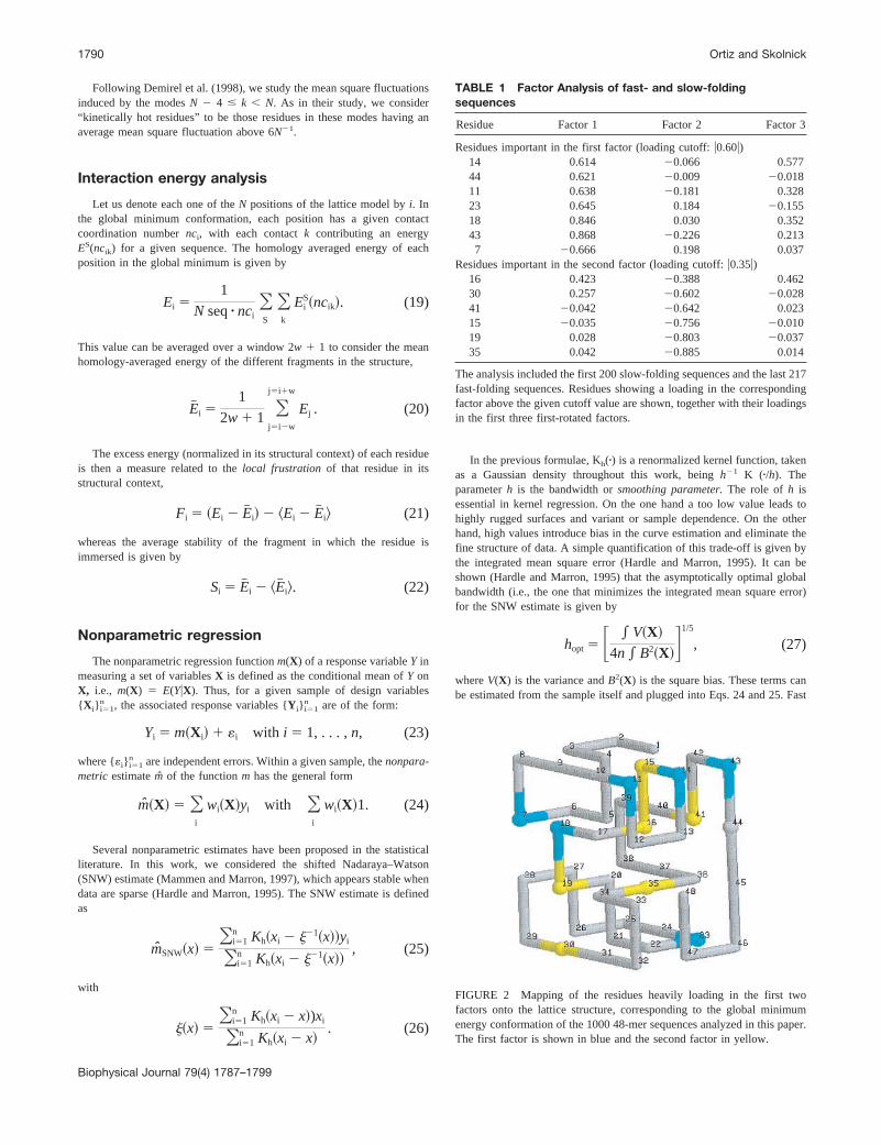
FIGURE 2 Mapping of the residues heavily loading in the first twofactors onto the lattice structure, corresponding to the global minimumenergy conformation of the 1000 48-mer sequences analyzed in this paper.The first factor is shown in blue and the second factor in yellow.

TABLE 1 Factor Analysis of fast- and slow-foldingsequences

Residue Factor 1 Factor 2 Factor 3

Residues important in the first factor (loading cutoff:u0.60u)14 0.614 20.066 0.57744 0.621 20.009 20.01811 0.638 20.181 0.32823 0.645 0.184 20.15518 0.846 0.030 0.35243 0.868 20.226 0.2137 20.666 0.198 0.037

Residues important in the second factor (loading cutoff:u0.35u)16 0.423 20.388 0.46230 0.257 20.602 20.02841 20.042 20.642 0.02315 20.035 20.756 20.01019 0.028 20.803 20.03735 0.042 20.885 0.014

The analysis included the first 200 slow-folding sequences and the last 217fast-folding sequences. Residues showing a loading in the correspondingfactor above the given cutoff value are shown, together with their loadingsin the first three first-rotated factors.



and simple estimates of these functions can be obtained based on polyno-mials and histograms, respectively. In the present work, theblock methodof Hardle and Marron (1995) for the estimates of the bias and varianceappearing in Eq. 27 proved to be robust. This method is based on dividingthe sample in histograms or blocks and fitting a low degree polynomial ineach block.

RESULTS

Analysis of the lattice protein models

Sequence factor analysis

We start by trying to identify from the sequences, byusing multivariate analysis, clusters of positions that canaccount for the kinetic differences between slow and fastfolding lattice proteins. Fig. 1 and Table 1 summarize theresults of an FA (Reyment and Joreskog, 1996) (see Meth-

ods for description of this multivariate technique) applied tothe fast and slow folding protein sequences. The first 200slow-folding and the last 217 fast-folding sequences weresubjected to the analysis. In Fig. 1,A and B, the originalsequence space spanned by the 2001 217 5 417 alignedsequences is projected onto the first two dimensions orfactors (Fig. 1B), or onto the first and third dimension (Fig.2). In Fig. 1, loadings are represented as diamonds, whereasscores are represented as lines (see Methods for definitionsof loadings and scores). These lines connect the 417 se-quences following the in silico evolutionary time of theevolutionary experiment. Sequences in the alignment areclassified into three groups: slow-folding sequences (repre-sented by a blue line), fast-folding sequences (red line), andvery-fast-folding sequences (magenta line). Note that thecoordinates of the line points in the second factor are verydifferent for slow- and fast-folding sequences, i.e., thepoints of these two groups of sequences are well separatedalong this axis. Also, there is some separation along the firstfactor of the very-fast-folding sequences from the rest.Finally, note that there is no significant discrimination alongthe third factor (Fig. 1B). Thus, this analysis suggests that,at the sequence level, the main differences in the kineticbehavior of the lattice proteins can be explained by twounderlying factors.

The first factor, explaining a higher proportion of thevariance, is what we call theloop factor,because residuesheavily loading in the first component are loop residues(Fig. 2). Within the loop residues, two types of positions canbe distinguished, evolving in an anticorrelated fashion: po-sition #7 becomes more hydrophilic, whereas the rest ofresidues become more hydrophobic. The later are in contactand apparently are required to fix or stabilize the loop

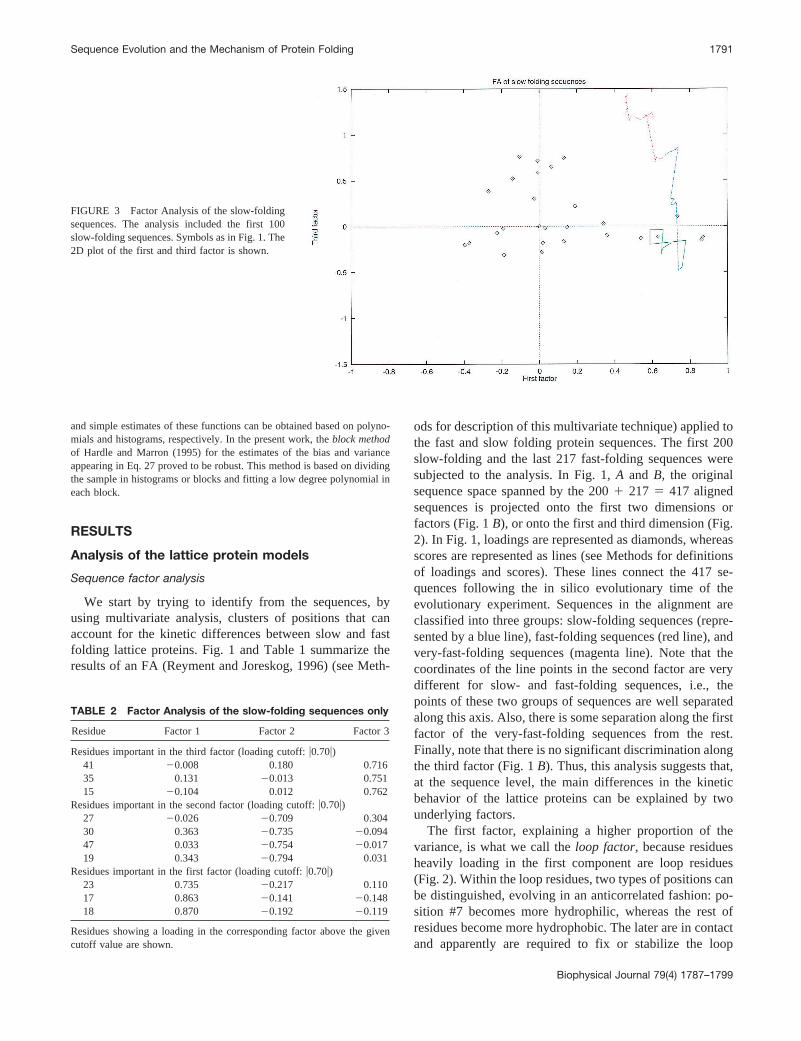
FIGURE 3 Factor Analysis of the slow-foldingsequences. The analysis included the first 100slow-folding sequences. Symbols as in Fig. 1. The2D plot of the first and third factor is shown.

TABLE 2 Factor Analysis of the slow-folding sequences only

Residue Factor 1 Factor 2 Factor 3

Residues important in the third factor (loading cutoff:u0.70u)41 20.008 0.180 0.71635 0.131 20.013 0.75115 20.104 0.012 0.762

Residues important in the second factor (loading cutoff:u0.70u)27 20.026 20.709 0.30430 0.363 20.735 20.09447 0.033 20.754 20.01719 0.343 20.794 0.031

Residues important in the first factor (loading cutoff:u0.70u)23 0.735 20.217 0.11017 0.863 20.141 20.14818 0.870 20.192 20.119

Residues showing a loading in the corresponding factor above the givencutoff value are shown.



conformation, whereas the former possibly avoids compet-ing interactions with the core, making the energy landscapeless rugged. Karplus and coworkers (Dinner et al., 1998)have recently obtained similar conclusions for a differentsystem using a different potential energy function. How-ever, they observed that only the weakening of interactionsbetween noncore residues increases the folding rate.

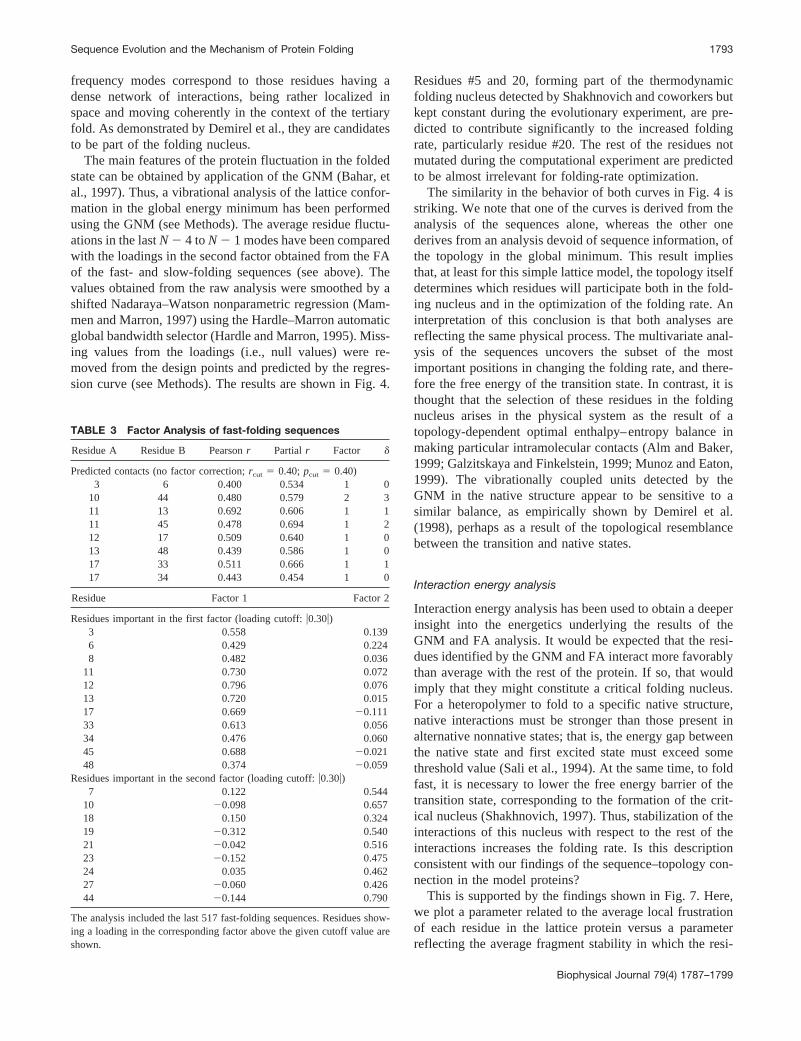
The second factor accounting for a high proportion of thevariance is thenucleus factor.A subset of the residuesbelonging to the previously detected thermodynamic fold-ing nucleus (Mirny et al., 1998) is found here (Fig. 2).However, not all the residues previously described as beingpart of the folding nucleus are discriminating (compare theyellow residues in Fig. 2 with the red residues in Fig. 5).This is, in part, the result of complete conservation of someof these residues between fast- and slow-folding sequences(e.g., for residues #5 and 20). There are also some excep-tions, for example, with residue #16. In contrast, residues#19 and 30 contribute to the differences in rate, but are notpart of the thermodynamic folding nucleus.

It is important to note that the ranking of factors obtainedfrom the FA model only reflects the fact that there are morerepresentatives of the medium- and fast-folding sequencesthan of the slow-folding ones, resulting from the fast opti-mization of the folding rate during the first mutations. Thus,from the viewpoint of explaining the covariance structure,the loop factor is more important (i.e., accounts for a higherproportion of the variance) than the nucleus factor. How-ever, the nucleus factor is far more important in its ability todiscriminate fast- from slow-folding sequences, whereas theloop factor only makes a modest contribution. This is evi-denced by the separation of the fast- and slow-foldingproteins along both axes.

To confirm the results of this analysis, it is also of interestto carry out an FA using the slow-folding sequences alone.Figure 3 and Table 2 show the results. The analysis indi-cates that the third factor can explain the fast increment inthe folding rate of the sequences (Fig. 3), whereas the firsttwo factors have much less explanatory power. Residuesloading in Factor 3 (Table 2) are mainly a subset of thoseresidues (#15, 41, and 35) also identified as being part of thethermodynamic folding nucleus by Shakhnovich and co-workers (Mirny, et al., 1998) (Fig. 5).

Thus, differences in kinetic behavior of the model pro-teins originate from sequence differences detectable by mul-tivariate analysis of the alignments. Folding rate is opti-mized rapidly, with the bulk of the optimization dependingonly on mutations in a small number of residues, a subset ofthe thermodynamic folding nucleus. Once this nucleus isstabilized, a slight increment in folding rate can be achievedby loop mutations.

Structural vibrational analysis

Following the ideas of Demirel et al. (1998), we identifythose residues from the protein structure which can bedescribed as beingkinetically hot.By this, we mean thatthese residues present a high vibrational frequency in thefolded state, implying that their motion is of small ampli-tude. This is a signature of a steep potential energy surfacearound their mean position, which arises from the contactcoordination number of the residue and the topologicalrestrictions imposed by the structure. The vibrations of thewhole structure can be decomposed into modes, with allresidues vibrating in a particular mode presenting concertedmotions. Thus, residues forming part of the same high-

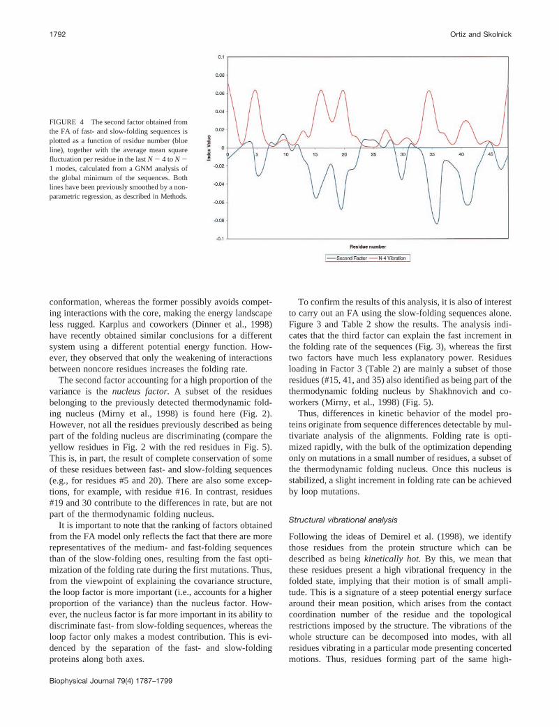
FIGURE 4 The second factor obtained fromthe FA of fast- and slow-folding sequences isplotted as a function of residue number (blueline), together with the average mean squarefluctuation per residue in the lastN 2 4 toN 21 modes, calculated from a GNM analysis ofthe global minimum of the sequences. Bothlines have been previously smoothed by a non-parametric regression, as described in Methods.



frequency modes correspond to those residues having adense network of interactions, being rather localized inspace and moving coherently in the context of the tertiaryfold. As demonstrated by Demirel et al., they are candidatesto be part of the folding nucleus.

The main features of the protein fluctuation in the foldedstate can be obtained by application of the GNM (Bahar, etal., 1997). Thus, a vibrational analysis of the lattice confor-mation in the global energy minimum has been performedusing the GNM (see Methods). The average residue fluctu-ations in the lastN 2 4 toN 2 1 modes have been comparedwith the loadings in the second factor obtained from the FAof the fast- and slow-folding sequences (see above). Thevalues obtained from the raw analysis were smoothed by ashifted Nadaraya–Watson nonparametric regression (Mam-men and Marron, 1997) using the Hardle–Marron automaticglobal bandwidth selector (Hardle and Marron, 1995). Miss-ing values from the loadings (i.e., null values) were re-moved from the design points and predicted by the regres-sion curve (see Methods). The results are shown in Fig. 4.

Residues #5 and 20, forming part of the thermodynamicfolding nucleus detected by Shakhnovich and coworkers butkept constant during the evolutionary experiment, are pre-dicted to contribute significantly to the increased foldingrate, particularly residue #20. The rest of the residues notmutated during the computational experiment are predictedto be almost irrelevant for folding-rate optimization.

The similarity in the behavior of both curves in Fig. 4 isstriking. We note that one of the curves is derived from theanalysis of the sequences alone, whereas the other onederives from an analysis devoid of sequence information, ofthe topology in the global minimum. This result impliesthat, at least for this simple lattice model, the topology itselfdetermines which residues will participate both in the fold-ing nucleus and in the optimization of the folding rate. Aninterpretation of this conclusion is that both analyses arereflecting the same physical process. The multivariate anal-ysis of the sequences uncovers the subset of the mostimportant positions in changing the folding rate, and there-fore the free energy of the transition state. In contrast, it isthought that the selection of these residues in the foldingnucleus arises in the physical system as the result of atopology-dependent optimal enthalpy–entropy balance inmaking particular intramolecular contacts (Alm and Baker,1999; Galzitskaya and Finkelstein, 1999; Munoz and Eaton,1999). The vibrationally coupled units detected by theGNM in the native structure appear to be sensitive to asimilar balance, as empirically shown by Demirel et al.(1998), perhaps as a result of the topological resemblancebetween the transition and native states.

Interaction energy analysis

Interaction energy analysis has been used to obtain a deeperinsight into the energetics underlying the results of theGNM and FA analysis. It would be expected that the resi-dues identified by the GNM and FA interact more favorablythan average with the rest of the protein. If so, that wouldimply that they might constitute a critical folding nucleus.For a heteropolymer to fold to a specific native structure,native interactions must be stronger than those present inalternative nonnative states; that is, the energy gap betweenthe native state and first excited state must exceed somethreshold value (Sali et al., 1994). At the same time, to foldfast, it is necessary to lower the free energy barrier of thetransition state, corresponding to the formation of the crit-ical nucleus (Shakhnovich, 1997). Thus, stabilization of theinteractions of this nucleus with respect to the rest of theinteractions increases the folding rate. Is this descriptionconsistent with our findings of the sequence–topology con-nection in the model proteins?

This is supported by the findings shown in Fig. 7. Here,we plot a parameter related to the average local frustrationof each residue in the lattice protein versus a parameterreflecting the average fragment stability in which the resi-

TABLE 3 Factor Analysis of fast-folding sequences

Residue A Residue B Pearsonr Partial r Factor d

Predicted contacts (no factor correction;rcut 5 0.40;pcut 5 0.40)3 6 0.400 0.534 1 0

10 44 0.480 0.579 2 311 13 0.692 0.606 1 111 45 0.478 0.694 1 212 17 0.509 0.640 1 013 48 0.439 0.586 1 017 33 0.511 0.666 1 117 34 0.443 0.454 1 0

Residue Factor 1 Factor 2

Residues important in the first factor (loading cutoff:u0.30u)3 0.558 0.1396 0.429 0.2248 0.482 0.036

11 0.730 0.07212 0.796 0.07613 0.720 0.01517 0.669 20.11133 0.613 0.05634 0.476 0.06045 0.688 20.02148 0.374 20.059

Residues important in the second factor (loading cutoff:u0.30u)7 0.122 0.544

10 20.098 0.65718 0.150 0.32419 20.312 0.54021 20.042 0.51623 20.152 0.47524 0.035 0.46227 20.060 0.42644 20.144 0.790

The analysis included the last 517 fast-folding sequences. Residues show-ing a loading in the corresponding factor above the given cutoff value areshown.



due is immersed (see Methods). A strong segregation ofresidues can be observed for the fast-folding sequenceswhen compared with the slow-folding ones: in the fast-folding sequences, most of residues are close to inert, withslightly repulsive environments and with a small value offrustration. Among the group of residues with low values oflocal frustration are residues #16, 41, and 20, all of themimportant in increasing the folding rate (Fig. 4), with resi-

dues #41 and 16 forming a contact and loading together inthe FA. Thus, during the optimization of the folding rate,strong favorable interactions are placed between these res-idues of the folding nucleus, and mild repulsive or inertinteractions (with respect to the average) are placed else-where. These results support the picture of the sequence–topology connection and suggest that a way to engineer fastfolding in real proteins is to select the kinetically hot resi-dues determined by the vibrational analysis of the topologyand then to optimize only the interactions of these residues.

Presence of correlated mutations

After the folding rate is optimized, accepted mutations willtend to minimally perturb the stability of the critical nu-cleus. This foldability requirement should tend to createrestrictions in sequence space. It is becoming well estab-lished that residues forming part of the folding nucleus tendto be conserved (Ptitsyn, 1998; Shakhnovich, et al., 1996),but it is also possible to imagine some other, more subtlerestrictions imposed by the folding nucleus. Thus, the mu-tational behavior of other residues outside the nucleus couldalso be restricted in varying degrees, creating patterns ofvariability, for example, in the form of correlations. Indeed,Table 3 and Fig. 6 show that correlated mutations emergefrom the set of evolutionary related sequences under fastfolding pressure. Most important, the residues involved incorrelation are either forming contacts or shifted in se-quence by, at most, two residues in contact map space(Table 4).

FIGURE 5 Display of the predicted contacts for the model sequencesusing an alignment based on the last 517 fast-folding sequences. Predictedcontacts are shown as dotted lines connecting the corresponding residues.Positions in red correspond to the residues participating in the thermody-namic folding nucleus as described by Shakhnovich and coworkers (Mirnyet al., 1998).

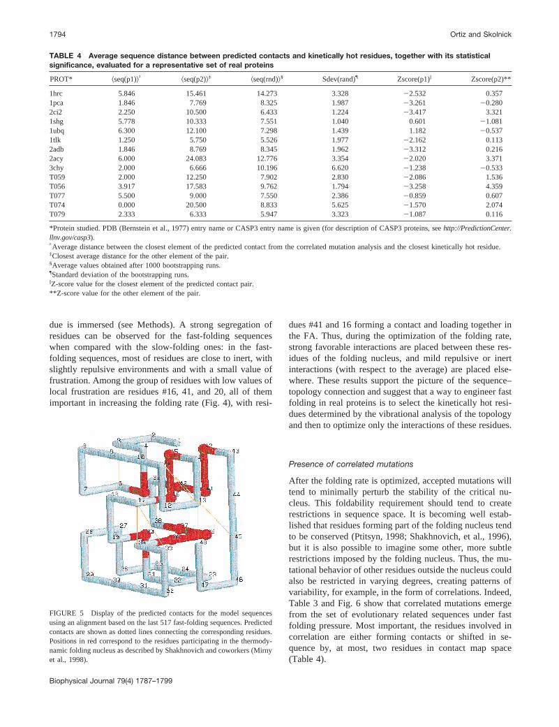
TABLE 4 Average sequence distance between predicted contacts and kinetically hot residues, together with its statisticalsignificance, evaluated for a representative set of real proteins

PROT* ^seq(p1)&† ^seq(p2)&‡ ^seq(rnd)&§ Sdev(rand)¶ Zscore(p1)\ Zscore(p2)**

1hrc 5.846 15.461 14.273 3.328 22.532 0.3571pca 1.846 7.769 8.325 1.987 23.261 20.2802ci2 2.250 10.500 6.433 1.224 23.417 3.3211shg 5.778 10.333 7.551 1.040 0.601 21.0811ubq 6.300 12.100 7.298 1.439 1.182 20.5371tlk 1.250 5.750 5.526 1.977 22.162 0.1132adb 1.846 8.769 8.345 1.962 23.312 0.2162acy 6.000 24.083 12.776 3.354 22.020 3.3713chy 2.000 6.666 10.196 6.620 21.238 20.533T059 2.000 12.250 7.902 2.830 22.086 1.536T056 3.917 17.583 9.762 1.794 23.258 4.359T077 5.500 9.000 7.550 2.386 20.859 0.607T074 0.000 20.500 8.833 5.625 21.570 2.074T079 2.333 6.333 5.947 3.323 21.087 0.116

*Protein studied. PDB (Bernstein et al., 1977) entry name or CASP3 entry name is given (for description of CASP3 proteins, seehttp://PredictionCenter.llnv.gov/casp3).†Average distance between the closest element of the predicted contact from the correlated mutation analysis and the closest kinetically hot residue.‡Closest average distance for the other element of the pair.§Average values obtained after 1000 bootstrapping runs.¶Standard deviation of the bootstrapping runs.\Z-score value for the closest element of the predicted contact pair.**Z-score value for the other element of the pair.



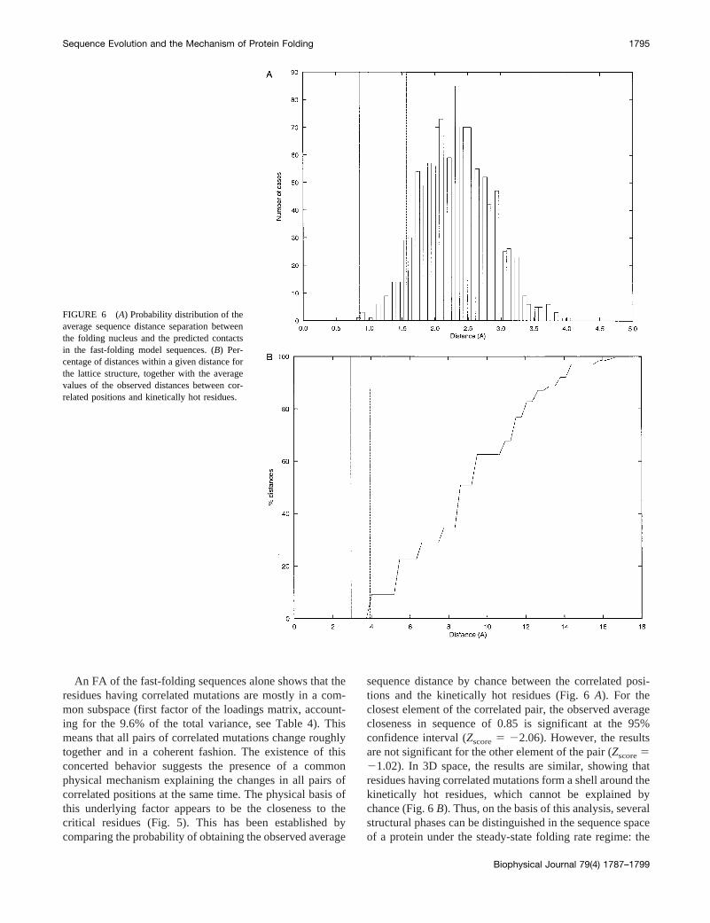
An FA of the fast-folding sequences alone shows that theresidues having correlated mutations are mostly in a com-mon subspace (first factor of the loadings matrix, account-ing for the 9.6% of the total variance, see Table 4). Thismeans that all pairs of correlated mutations change roughlytogether and in a coherent fashion. The existence of thisconcerted behavior suggests the presence of a commonphysical mechanism explaining the changes in all pairs ofcorrelated positions at the same time. The physical basis ofthis underlying factor appears to be the closeness to thecritical residues (Fig. 5). This has been established bycomparing the probability of obtaining the observed average

sequence distance by chance between the correlated posi-tions and the kinetically hot residues (Fig. 6A). For theclosest element of the correlated pair, the observed averagecloseness in sequence of 0.85 is significant at the 95%confidence interval (Zscore5 22.06). However, the resultsare not significant for the other element of the pair (Zscore521.02). In 3D space, the results are similar, showing thatresidues having correlated mutations form a shell around thekinetically hot residues, which cannot be explained bychance (Fig. 6B). Thus, on the basis of this analysis, severalstructural phases can be distinguished in the sequence spaceof a protein under the steady-state folding rate regime: the

FIGURE 6 (A) Probability distribution of theaverage sequence distance separation betweenthe folding nucleus and the predicted contactsin the fast-folding model sequences. (B) Per-centage of distances within a given distance forthe lattice structure, together with the averagevalues of the observed distances between cor-related positions and kinetically hot residues.



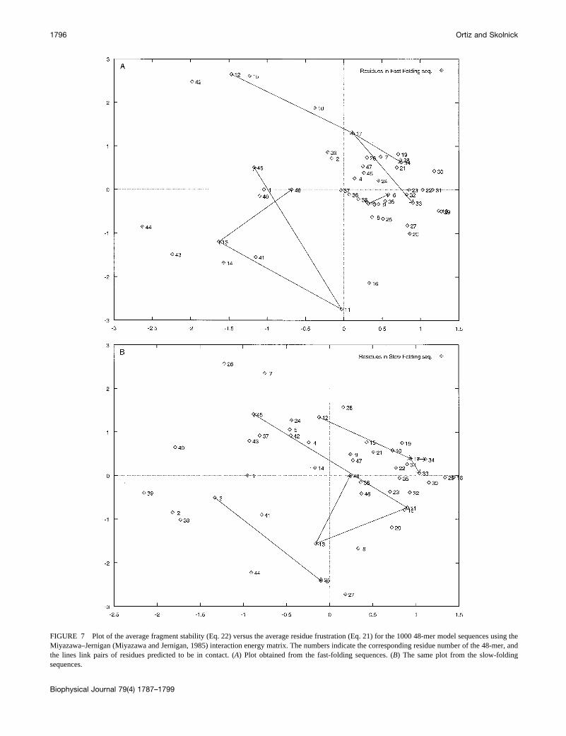
FIGURE 7 Plot of the average fragment stability (Eq. 22) versus the average residue frustration (Eq. 21) for the 1000 48-mer model sequences using theMiyazawa–Jernigan (Miyazawa and Jernigan, 1985) interaction energy matrix. The numbers indicate the corresponding residue number of the 48-mer, andthe lines link pairs of residues predicted to be in contact. (A) Plot obtained from the fast-folding sequences. (B) The same plot from the slow-foldingsequences.



(almost) conserved folding nucleus, the shell of residuesaround it involved in correlated mutations, and the rest ofresidues mutating (almost) independently.

Analysis of real proteins

We were interested to see whether there is a qualitativecorrespondence between the results obtained with the latticeproteins and what can be observed in real proteins. Al-

though the situation with real proteins is more complex, atleast a qualitative agreement should be obtained. For suchcomparison to be meaningful, the same computational pro-cedures should be applied in both cases, with the samecoarse graining. Thus, core residues were automaticallyselected from the 3D structure in the same way it was donefor the lattice proteins, based on the GNM calculations,while correlations in the alignments were also computedfollowing the same procedure used with the lattice proteins.

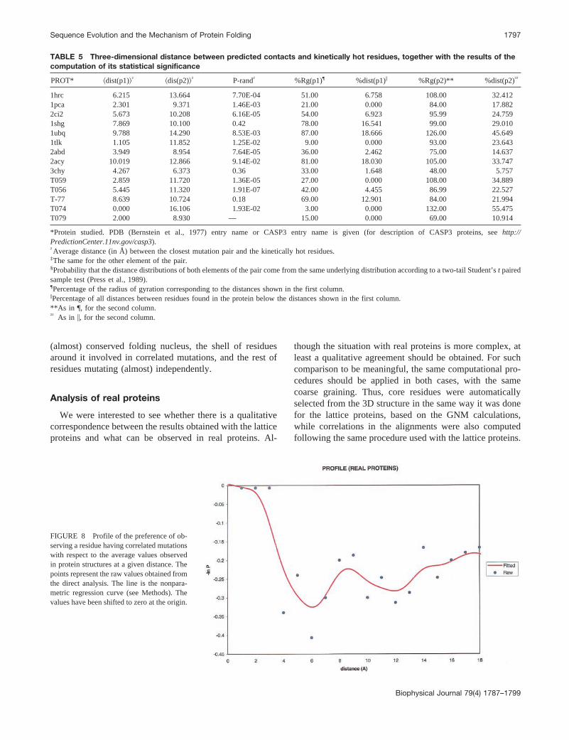
FIGURE 8 Profile of the preference of ob-serving a residue having correlated mutationswith respect to the average values observedin protein structures at a given distance. Thepoints represent the raw values obtained fromthe direct analysis. The line is the nonpara-metric regression curve (see Methods). Thevalues have been shifted to zero at the origin.

TABLE 5 Three-dimensional distance between predicted contacts and kinetically hot residues, together with the results of thecomputation of its statistical significance

PROT* ^dist(p1)&† ^dis(p2)&† P-rand† %Rg(p1)¶ %dist(p1)\ %Rg(p2)** %dist(p2)††

1hrc 6.215 13.664 7.70E-04 51.00 6.758 108.00 32.4121pca 2.301 9.371 1.46E-03 21.00 0.000 84.00 17.8822ci2 5.673 10.208 6.16E-05 54.00 6.923 95.99 24.7591shg 7.869 10.100 0.42 78.00 16.541 99.00 29.0101ubq 9.788 14.290 8.53E-03 87.00 18.666 126.00 45.6491tlk 1.105 11.852 1.25E-02 9.00 0.000 93.00 23.6432abd 3.949 8.954 7.64E-05 36.00 2.462 75.00 14.6372acy 10.019 12.866 9.14E-02 81.00 18.030 105.00 33.7473chy 4.267 6.373 0.36 33.00 1.648 48.00 5.757T059 2.859 11.720 1.36E-05 27.00 0.000 108.00 34.889T056 5.445 11.320 1.91E-07 42.00 4.455 86.99 22.527T-77 8.639 10.724 0.18 69.00 12.901 84.00 21.994T074 0.000 16.106 1.93E-02 3.00 0.000 132.00 55.475T079 2.000 8.930 — 15.00 0.000 69.00 10.914

*Protein studied. PDB (Bernstein et al., 1977) entry name or CASP3 entry name is given (for description of CASP3 proteins, seehttp://PredictionCenter.11nv.gov/casp3).†Average distance (in Å) between the closest mutation pair and the kinetically hot residues.‡The same for the other element of the pair.§Probability that the distance distributions of both elements of the pair come from the same underlying distribution according to a two-tail Student’s t pairedsample test (Press et al., 1989).¶Percentage of the radius of gyration corresponding to the distances shown in the first column.\Percentage of all distances between residues found in the protein below the distances shown in the first column.**As in ¶, for the second column.†† As in \, for the second column.



We created a test set including proteins for which experi-mental data about their folding nucleus were available, aswell as proteins for which contacts were predicted blindly,in advance of the knowledge of the structure, during therecent CASP3 contest (http://PredictionCenter.llnv.gov/casp3) (see Ortiz et al., 1999).

Contacts are predicted from the MSAs as described (Ortizet al., 1999) (see Methods). Overall, the prediction accuracyin this small sample is similar to that obtained when a largernumber of proteins was used when developing the predic-tion method. Thus, most of the predicted contacts havecorrespondence with a real contact within a local sequencewindow of d 5 3 (data not shown). In contrast, from thetopology of the protein, a vibrational analysis with the GNMwas conducted as described (Bahar, et al., 1997). In agree-ment with Demirel et al. (1998), we observe a statisticallysignificant overlap between the experimentally describedfolding nucleus and the kinetically hot residues (data notshown). Similar to the results obtained with the latticeprotein, we also observe a statistically significant shortsequence distance between the closest element of the pre-dicted contact from the correlated mutation analysis and theclosest kinetically hot residue (Table 4), although this is notthe case for the second element of the pair (Table 4). Similarresults were obtained when analyzing the relationship in 3Dspace. Thus, it is found that residues from the closestmember of a correlated mutation pair tend to appear in thefirst coordination shell of a kinetically hot residue moreoften than expected by chance (see Table 5 and Fig. 8). Asomewhat weaker tendency is observed for the second ele-ment, which tends to be located in the second solvation shellof the kinetically hot residues (Fig. 8) and in contact withthe first element of the pair. Both elements have signifi-

cantly different radial distribution functions with respect tothe kinetically hot residues (Table 5). A qualitative pictureof the relationships can be seen in Fig. 9.

CONCLUDING REMARKS

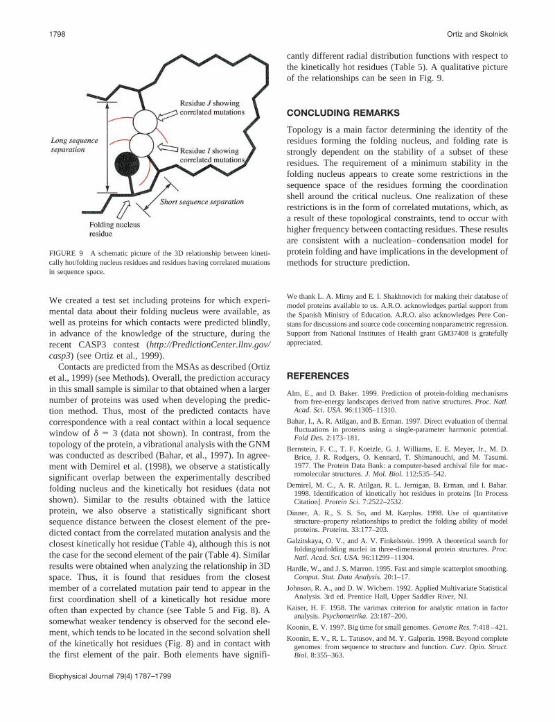
Topology is a main factor determining the identity of theresidues forming the folding nucleus, and folding rate isstrongly dependent on the stability of a subset of theseresidues. The requirement of a minimum stability in thefolding nucleus appears to create some restrictions in thesequence space of the residues forming the coordinationshell around the critical nucleus. One realization of theserestrictions is in the form of correlated mutations, which, asa result of these topological constraints, tend to occur withhigher frequency between contacting residues. These resultsare consistent with a nucleation–condensation model forprotein folding and have implications in the development ofmethods for structure prediction.

We thank L. A. Mirny and E. I. Shakhnovich for making their database ofmodel proteins available to us. A.R.O. acknowledges partial support fromthe Spanish Ministry of Education. A.R.O. also acknowledges Pere Con-stans for discussions and source code concerning nonparametric regression.Support from National Institutes of Health grant GM37408 is gratefullyappreciated.

REFERENCES

Alm, E., and D. Baker. 1999. Prediction of protein-folding mechanismsfrom free-energy landscapes derived from native structures.Proc. Natl.Acad. Sci. USA.96:11305–11310.

Bahar, I., A. R. Atilgan, and B. Erman. 1997. Direct evaluation of thermalfluctuations in proteins using a single-parameter harmonic potential.Fold Des.2:173–181.

Bernstein, F. C., T. F. Koetzle, G. J. Williams, E. E. Meyer, Jr., M. D.Brice, J. R. Rodgers, O. Kennard, T. Shimanouchi, and M. Tasumi.1977. The Protein Data Bank: a computer-based archival file for mac-romolecular structures.J. Mol. Biol. 112:535–542.

Demirel, M. C., A. R. Atilgan, R. L. Jernigan, B. Erman, and I. Bahar.1998. Identification of kinetically hot residues in proteins [In ProcessCitation]. Protein Sci.7:2522–2532.

Dinner, A. R., S. S. So, and M. Karplus. 1998. Use of quantitativestructure–property relationships to predict the folding ability of modelproteins.Proteins.33:177–203.

Galzitskaya, O. V., and A. V. Finkelstein. 1999. A theoretical search forfolding/unfolding nuclei in three-dimensional protein structures.Proc.Natl. Acad. Sci. USA.96:11299–11304.

Hardle, W., and J. S. Marron. 1995. Fast and simple scatterplot smoothing.Comput. Stat. Data Analysis.20:1–17.

Johnson, R. A., and D. W. Wichern. 1992. Applied Multivariate StatisticalAnalysis. 3rd ed. Prentice Hall, Upper Saddler River, NJ.

Kaiser, H. F. 1958. The varimax criterion for analytic rotation in factoranalysis.Psychometrika.23:187–200.

Koonin, E. V. 1997. Big time for small genomes.Genome Res.7:418–421.

Koonin, E. V., R. L. Tatusov, and M. Y. Galperin. 1998. Beyond completegenomes: from sequence to structure and function.Curr. Opin. Struct.Biol. 8:355–363.

FIGURE 9 A schematic picture of the 3D relationship between kineti-cally hot/folding nucleus residues and residues having correlated mutationsin sequence space.



Mammen, E., and J. S. Marron. 1997. Mass recentered kernel smoothers.Biometrika.84:765–777.

Mirny, L. A., V. I. Abkevich, and E. I. Shakhnovich. 1998. How evolutionmakes proteins fold quickly.Proc. Natl. Acad. Sci. USA.95:4976–4981.

Miyazawa, S., and R. L. Jernigan. 1985. Estimation of effective interresi-due contact energies from protein crystal structures: quasi-chemicalapproximation.Macromolecules.18:534–552.

Munoz, V., and W. A. Eaton. 1999. A simple model for calculating thekinetics of protein folding from three-dimensional structures.Proc. Natl.Acad. Sci. USA.96:11311–11316.

Ortiz, A. R., A. Kolinski, P. Rotkiewicz, B. Ilkowski, and J. Skolnick.1999. Ab initio folding of proteins using restraints derived from evolu-tionary information.Proteins.(Suppl.) 3:177–185.

Press, W. H., B. P. Flannery, S. A. Teukolsky, and W. T. Vetterling. 1989.Numerical Recipes. The Art of Scientific Computing. Cambridge Uni-versity Press.

Ptitsyn, O. B. 1998. Protein folding and protein evolution: common foldingnucleus in different subfamilies of c-type cytochromes?J. Mol. Biol.278:655–666.

Reyment, R., and K. G. Joreskog. 1996. Applied Factor Analysis in theNatural Sciences. Cambridge University Press.

Sali, A., E. Shakhnovich, and M. Karplus. 1994. How does a protein fold?Nature.369:248–251.

Sander, C., and R. Schneider. 1991. Database of homology derived proteinstructures and the structural meaning of sequence alignment.Proteins.9:56–68.

Shakhnovich, E. I. 1996. Modeling protein folding: the beauty and powerof simplicity. Fold. Design.1:R50–R54.

Shakhnovich, E. 1997. Theoretical studies of protein folding thermody-namics and kinetics.Curr. Opin. Struct. Biol.7:29–40.

Shakhnovich, E., V. Abkevich, and O. Ptitsyn. 1996. Conserved residuesand the mechanism of protein folding.Nature.379:96–98.



Documents

Sequence Evolution and the Mechanism of Protein Folding