Separating the Wheat from the Chaff: Finding a Concensus

Prediction For the Strength of Solar Cycle 24

D.A. BieseckerNOAA/SEC

It’s not the predictions

• Wheat– E. Kihn– M. Dikpati– D. Hathaway– D. Pesnell– T. Hoeksema– L. Svalgaard– R. van der Linden– H. Lundstedt– R. Thompson– DOD Representative– O.C. St. Cyr ex officio– J. Kunches ex officio

• Chaff– Biesecker

The panel will convene for the first time in OctoberPreliminary Prediction due in April, 2007

Overview

• What the heck do I know?• Who wants to know about the next solar cycle

– Pretty much everyone– Why?

• What are some of the prediction techniques– Statistical– Precursor

• What else is out there?– Sudden Turn-on– The skeptics

• Coming up with a consensus prediction– How did the last panel do?

Who wants a prediction?

• Almost everyone, it seems– Satellite operators

• Mission planning– 18 year predictions (1 yr study, 2-yr build, 15-yr

mission)• Parts selection

– Want to use previously qualified components» Don’t want to qualify components for a more

severe environment unnecessarily• Insurance costs

– Mission lifetime and premature failures

– NASA– DOD

Who wants a prediction?

– HF Communications• Small cycle – fewer available frequencies• Lots of activity – more interruptions

– Ham operators – the last line of defense in communications

– Want to know how many storms to expect• Electric Utilities• Media• And pretty much everyone else

Effect of Solar X-rays on D-Region and HF Propagation.

• D-Region Absorption Product based on GOES X-Ray Flux (SEC Product)– The map shows regions affected by the increased D-region ionization resulting

from enhanced x-ray flux during magnitude X-1 Flare

What is an average solar cycle?

• Avg is 11.0±1.5 yrs [8.2, 15]• Peak is 113.7±39.5 [48.7, 164.5]• Rise to Max is 4.7±1.4 yrs [2.8, 7.5]• Fall to Min is 6.3±1.3 yrs [3.5, 10.2]

– Isn’t this good enough for predicting?

What predictions are out there?

• Precursor, Spectral Analysis, Climatology, Recent Climatology, Neural Network…

• As of May 5, 2006

• 11 published so far– 8 below average– 3 above average

Author Year of Publication

Peak SSN

Hathaway et al.

1999 Strong

Dikpati et al. 2006 >155

Gholipour et al.

2005 145

Kane 1999 105

Wang et al. 2002 101

Duhau 2003 88

Schatten 2005 80

Svalgaard 2005 75

Badalyan et al. 2001 <50

Maris et al. 2004 Low

Clilverd et al. 2004 Weak

The Solar Cycle

Accurate Predictions by 30 MonthsAccurate Predictions by 30 Months

The amplitude and starting time, can be accurately determined by about The amplitude and starting time, can be accurately determined by about 30 months from the start of the cycle.30 months from the start of the cycle.

Doesn’t meet most ‘forecast’ requirementsDoesn’t meet most ‘forecast’ requirements

YEARS AFTER START OF CYCLE

Cycle 23 PredictionCycle 23 Prediction

Prediction at month 30Prediction at month 30

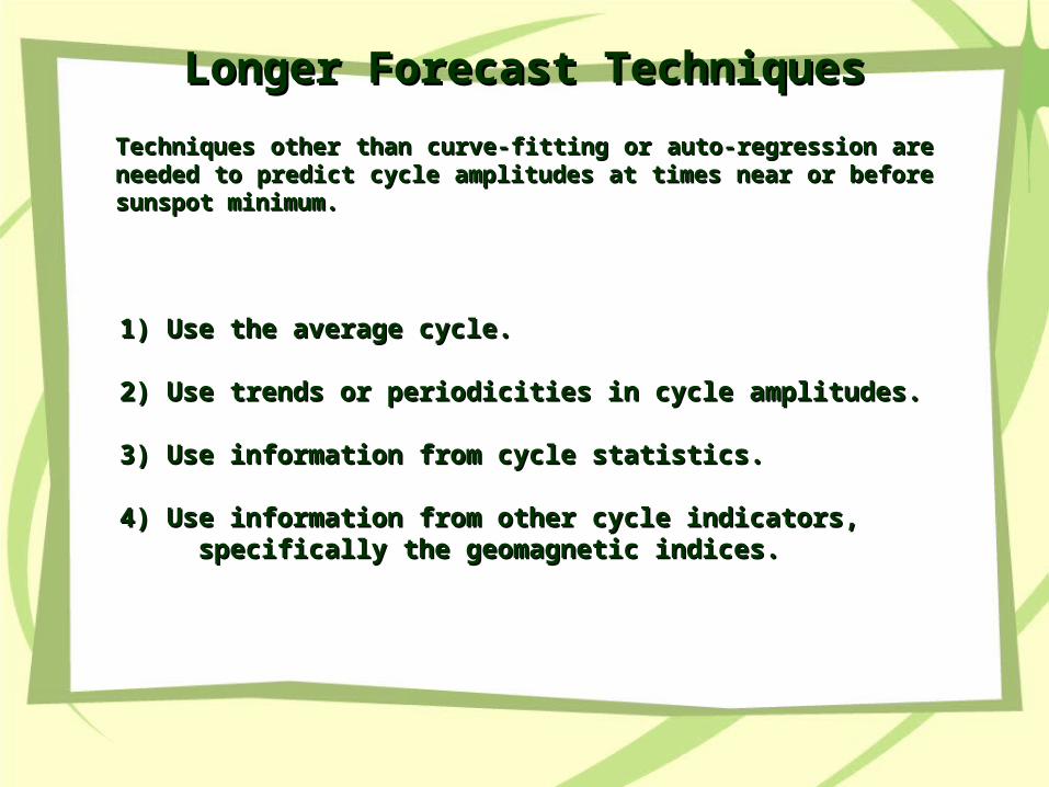
Longer Forecast TechniquesLonger Forecast Techniques

Techniques other than curve-fitting or auto-regression are needed to Techniques other than curve-fitting or auto-regression are needed to predict cycle amplitudes at times near or before sunspot minimum.predict cycle amplitudes at times near or before sunspot minimum.

1) Use the average cycle.1) Use the average cycle.

2) Use trends or periodicities in cycle amplitudes.2) Use trends or periodicities in cycle amplitudes.

3) Use information from cycle statistics. 3) Use information from cycle statistics.

4) Use information from other cycle indicators,4) Use information from other cycle indicators, specifically the geomagnetic indices.specifically the geomagnetic indices.

Secular Trend Since Maunder MinimumSecular Trend Since Maunder Minimum

The Group Sunspot Number shows a significant secular increase The Group Sunspot Number shows a significant secular increase in cycle amplitude since the Maunder Minimum.in cycle amplitude since the Maunder Minimum.

Multi-Cycle Periodicities?Multi-Cycle Periodicities?After removing the secular trend, there is little evidence for any After removing the secular trend, there is little evidence for any significant periodic behavior with periods of 2-cycles (Gnevyshev-Ohl) or significant periodic behavior with periods of 2-cycles (Gnevyshev-Ohl) or 3-cycles (Ahluwalia) There is some evidence for periodic behavior with a 3-cycles (Ahluwalia) There is some evidence for periodic behavior with a period of about 9-cycles (Gleissberg). period of about 9-cycles (Gleissberg).

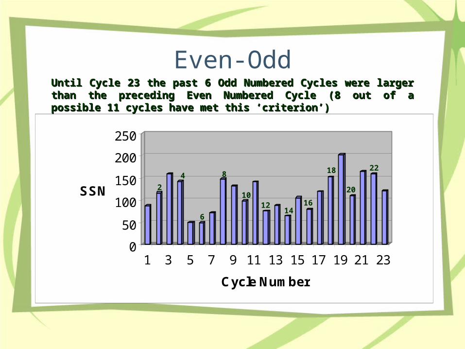
Even-Odd

0

50

100

150

200

250

SSN

1 3 5 7 9 11 13 15 17 19 21 23

Cycle Number

Until Cycle 23 the past 6 Odd Numbered Cycles were larger than the Until Cycle 23 the past 6 Odd Numbered Cycles were larger than the preceding Even Numbered Cycle (8 out of a possible 11 cycles have met preceding Even Numbered Cycle (8 out of a possible 11 cycles have met this ‘criterion’)this ‘criterion’)

22

20

18

1614

1210

8

6

4

2

Geomagnetic PrecursorsGeomagnetic PrecursorsGeomagnetic activity around the time of minimum seems to give an Geomagnetic activity around the time of minimum seems to give an indication of the size of the next maximum. indication of the size of the next maximum. •Ohl used Ohl used aaaa index index•Feynmann split the Feynmann split the aaaa index into two components index into two components•Thompson used only Thompson used only aa aa resulting from recurrent stormsresulting from recurrent storms

Prediction Method Cycle 19 Cycle 20 Cycle 21 Cycle 22 Cycle 23 RMSMean Cycle -94.8 -9.1 -53.5 -48.6 -10.1 53.7Secular Trend -91.6 8.7 -36.2 -25.3 17.8 46.3Gleissberg Cycle -80.4 18.5 -51.6 -51.1 -9.6 49.4Even-Odd -59.3 -22.3 61.1 50.8Amplitude-Period -74.1 0.3 -61.2 -25.3 9.7 44.7Maximum-Minimum -83.9 21.6 -22.9 -15.0 1.8 40.6Ohl's Method -55.4 19.1 21.8 4.4 22.2 29.7Feynmann's Method -42.8 9.6 26.9 3.6 41.1 29.5Thompson's Method -17.8 8.7 -26.5 -13.6 40.1 24.1

Prediction Method Errors (Prediction-Observed)Prediction Method Errors (Prediction-Observed)

Testing Precursor TechniquesTesting Precursor Techniques

1) Back up in time to the beginning of each of the last five cycles.1) Back up in time to the beginning of each of the last five cycles.

2) Using only information from earlier times, recalibrate each technique 2) Using only information from earlier times, recalibrate each technique and apply the results to that cycle.and apply the results to that cycle.

3) Compare the predictions with the actual numbers.3) Compare the predictions with the actual numbers.

Predicting the Solar Cycle With A Statistical Model

• Why not use a statistical model?– Climatology is a pretty standard

forecasting technique. If it’s happened before, it’s likely to happen again. • Wang et al. “The Prediction of Maximum

Amplitudes of Solar Cycles and the Maximum Amplitude of Solar Cycle 24” Chin. J. Astron. Astrophys. 2, 557-562, 2002.

A statistical method• An: ‘rise to max’

• Dn: ‘fall to min’

• Mn: sunspot number

• Kn: cycle length

Rise Time

SS

N

• SSN ~ Rise Time– HRV

• 1, 5, 7, 9, 19, 21

• M=312-37*An

– LRV• All even cycles and 3, 11, 13, 15, 17, 23

• M=263 – 38*An

Predicting Cycle 24

• K(n, n+1) = 1.95Dn-3.14– For cycles “Similar”

to 23• Based on M and A

• Cycle 24 is ‘Even’ so use LRV curve

• SSN = 101.3±18.1

Rise Time

SS

N

So lets look at dynamo based methods

• The basics– Large-scale polar fields on the decline of the solar

cycle are converted to poloidal field in the next cycle

• Strength of polar fields → peak of next cycle

Schematic summary of predictive flux-transport dynamo model

Shearing of poloidal fields by differential rotation to produce new toroidal fields, followed by

eruption of sunspots.

Spot-decay and spreading to produce new surface global

poloidal fields.

Transport of poloidal fields by meridional circulation (conveyor belt)

toward the pole and down to the bottom, followed by regeneration of new toroidal fields of opposite sign.

Courtesy of M. Dikpati

Precursor Method – Small CycleL. Svalgaard et al. (2005)

• Predicting a small Cycle 24– Even after the polar field reversal the old

polarity flux still holds on in the poles– Poleward moving fields don’t fully fill pole until

~3 years before solar minimum

Svalgaard et al. continued

• Dipole Moment = ABS(North – South)– Assume SSN=0 if

DM=0

• Fit Cycles 22 & 23– SSN = 0.6286*DM

• Cycle 24 DM (so far)– 119.3

• SSN = 75

Cycle DM(μTesla

)

Observed SSN

Predicted SSN

22 245.1 158.5 154.1

23 200.8 120.8 126.2

0

25

50

75

100

125

150

175

200

0 100 200 300 400

Dipole Moment (microTesla)

SS

N

Cycle 22

Cycle 23

Cycle 24

Precursor Method – Large CycleDikpati et al (2006)

• Flux Transport Dynamo– Fully account for meridional circulation– Circulation takes 17-21 years to

transport polar fields down to the shear layer

– So, cycle N is influenced by cycles N-1, N-2, and N-3

Large-scale dynamo processes

(i) Generation of toroidal (azimuthal) field by

shearing a pre-existing poloidal field

(component in meridional plane) by

differential rotation (Ω-effect )

(ii) Re-generation of poloidal field by lifting and twisting a toroidal flux tube

by helical turbulence (α-effect)

(iii) Flux transport by meridional circulation

= FLUX-TRANSPORT DYNAMO

<

Sun’s “memory” of past cycles controlled by

meridional circulation.

Dynamos with Meridional FlowDynamos with Meridional Flow

Recent Dynamo theories incorporate a deep meridional flow to transport Recent Dynamo theories incorporate a deep meridional flow to transport magnetic flux toward the equator at the base of the convection zone. They magnetic flux toward the equator at the base of the convection zone. They explain the equatorward drift of activity, the poleward drift of weak explain the equatorward drift of activity, the poleward drift of weak magnetic elements on the surface, length of the cycle from the speed of magnetic elements on the surface, length of the cycle from the speed of the flow, and give a relationship between polar fields at minimum and the the flow, and give a relationship between polar fields at minimum and the amplitude of future cycles.amplitude of future cycles.

Dikpati and Charbonneau, Dikpati and Charbonneau, ApJApJ 518, 508-520, 1999 518, 508-520, 1999

Hathaway finds the sunspot cycle period is anti-correlated with the drift Hathaway finds the sunspot cycle period is anti-correlated with the drift velocity at cycle maximum. The faster the drift rate the shorter the period. velocity at cycle maximum. The faster the drift rate the shorter the period.

R=-0.595% Significant

Drift Rate – Period Anti-correlationDrift Rate – Period Anti-correlation

Hathaway also finds that the drift velocity at cycle maximum is correlated Hathaway also finds that the drift velocity at cycle maximum is correlated to the amplitude of the second following (N+2) cycle maximum. The to the amplitude of the second following (N+2) cycle maximum. The correlation is much weaker for the immediately following maximum.correlation is much weaker for the immediately following maximum.

R=0.7R=0.799% Significant99% Significant

Drift Rate – Amplitude CorrelationsDrift Rate – Amplitude Correlations

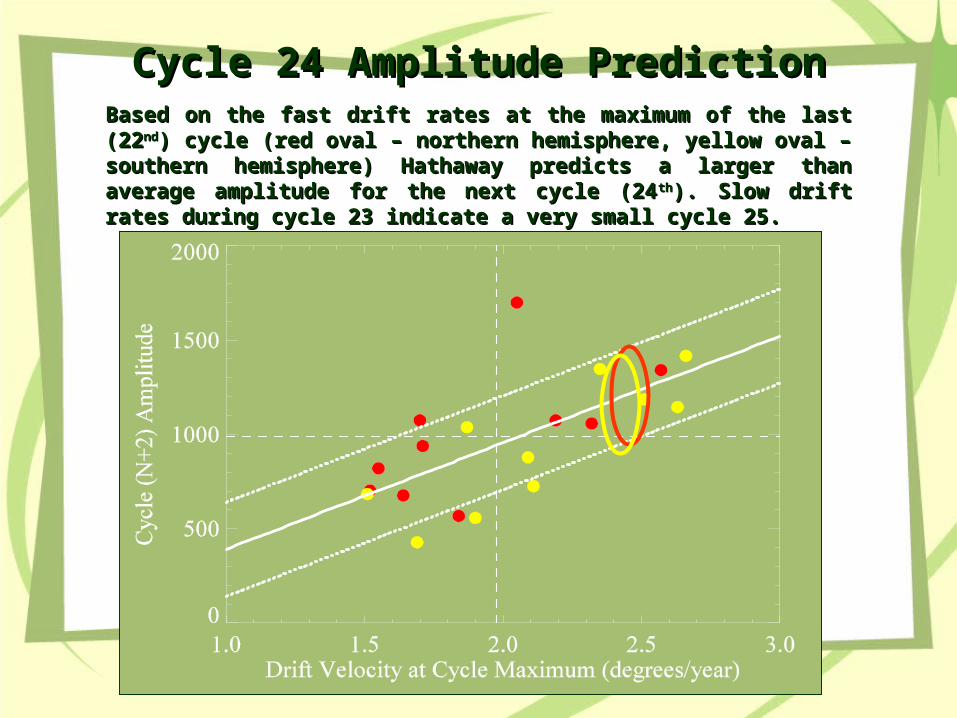
Cycle 24 Amplitude PredictionCycle 24 Amplitude PredictionBased on the fast drift rates at the maximum of the last (22Based on the fast drift rates at the maximum of the last (22ndnd) cycle (red ) cycle (red oval – northern hemisphere, yellow oval – southern hemisphere) oval – northern hemisphere, yellow oval – southern hemisphere) Hathaway predicts a larger than average amplitude for the next cycle Hathaway predicts a larger than average amplitude for the next cycle (24(24thth). Slow drift rates during cycle 23 indicate a very small cycle 25.). Slow drift rates during cycle 23 indicate a very small cycle 25.

Simulating relative peaks of cycles 12 through 24

(Dikpati, de Toma & Gilman, 2006)

• Dikpati et al. reproduce the peaks from cycle 16 through 23

• They predict cycle 24 will be 30-50% larger than cycle 23

• SSN = 157-181

Skeptic(s)

• Letter to Nature 442, 26 “Unpredictable Sun leaves researchers in the dark.” Tobias, S., Hughes, D., Weiss, N.– “The model proposed by Mausumi Dikpati and her team…

relies on parametrization of many poorly understood effects. Although such parametrized models have been widely (and legitimately) used to explore specific features of dynamo processes, they have no detailed predictive power. Indeed, there is vociferous debate in the field, not just about the size of many of the effects included in…many…people's models but even their signs. Moreover, the dynamo equations are extremely nonlinear; the solar dynamo is believed to exist in a state of deterministic chaos, making prediction intrinsically yet more difficult. Any predictions made with such models should be treated with extreme caution (or perhaps disregarded), as they lack solid physical underpinnings.”

The Yohkoh SXT DataDoes the activity turn on ‘instantly’?

Saba, Strong, and Slater• 72,000 full-disk thin Al filter

images– Passband: 3 to 50 Å – Temperature: 1 to 50 MK

• Selection towards the quieter times (<C-level flares)

• Complete, calibrated, aligned, despiked, and background subtracted

• Sum all pixels to get total X-ray flux

• Yields: one datum per image

Yohkoh Full-disk Image Taken in the Thin Aluminium Yohkoh Full-disk Image Taken in the Thin Aluminium Filter Filter

How Much Does the X-ray Sun Vary?

27-Day Running Average

Minimum

GOES XRS Confirms the SXT Result

• 5-min Averaged 1 – 8 A Data

• Found Minimum Flux for Each Day

– Selects against flares

• Found Similar Step as Seen by Yohkoh SXT

– Steps are simultaneous– XRS significantly

“harder” than SXT

Most of the New Activity Originates in the Active Region

Belt

Weak Fields Show Gradual Increase

Flare Rate Increases Sharply at Step

1

10

100

1000

Jan-97 Apr-97 Jul-97 Oct-97 Jan-98

Total Number of Flares (C + M + X)Total Number of Flares (C + M + X)

Weighted Number of Flares (C + 10*M + 100*X)Weighted Number of Flares (C + 10*M + 100*X)

In the 7 months before the step: 30 flaresIn the 7 months before the step: 30 flaresIn the 7 months after the step: 430 flaresIn the 7 months after the step: 430 flares

1911

1913

1915

1917

1919

1921

1923

1925

1927

1929

1931

1933

1935

OLD

0

1

2

3

4

5

6

7

8

9

10

OLD

NEW

No Old Cycle Regions Emerge After Step

Northern HemisphereDominant (55%)

Is it evident in Sunspot Statistics?•Monthly averaged sunspot area shows the stepSunspot Number Less Prominently

A Prediction

• Look at previous cycles – Available data types more

limited– Less coverage – Calibration less well

established

• The initial indications: Onsets of Cycles 21 and 22 also show similar steps, about 140 CRs apart

– Predict Next Step:

Jan 2008 (± 2 months)

Cycle 22 Cycle 23

GOES 1-8GOES 1-8 Å Minimum Daily Flux Å Minimum Daily Flux with 1-Month Boxcar Smoothwith 1-Month Boxcar Smooth

140 CRs(10.45 Years)

The Cycle 23 Prediction Panel• Joselyn et al., EOS 78, No. 20, 1997

Technique Low End High End

Even/Odd 165 235

Precursor 140 180

Spectral 135 185

Recent Climatology

125 185

Neural Networks

110 170

Climatology 75 155

The Cycle 23 Prediction

• “…the panel of 12 scientists…agreed that a large amplitude solar cycle with a smoothed sunspot maximum of approximately 160 is probable…”– Observed SSN = 120.8

• “The smoothed cycle maximum (before the date for the Cycle 23 minimum is confirmed) is predicted to occur in March 2000, within the range of January 1999 to June 2001”– Observed Maximum Date: March 2000

Summary

• The predictions for Cycle 24 are just as disparate as those for The predictions for Cycle 24 are just as disparate as those for Cycle 23, but the Cycle 23 consensus was for a LARGE cycleCycle 23, but the Cycle 23 consensus was for a LARGE cycle– Cycle 24 predictions from 50-160Cycle 24 predictions from 50-160

• Solar cycle predicting is growing ever more sophisticatedSolar cycle predicting is growing ever more sophisticated– This dynamo model must undergo independent tests to confirm This dynamo model must undergo independent tests to confirm

its abilities and to determine the effects of actual variations in its abilities and to determine the effects of actual variations in the meridional flow speed on predicted amplitudesthe meridional flow speed on predicted amplitudes

• It’s not apparent that any of the existing models will predict a It’s not apparent that any of the existing models will predict a Maunder Minimum and/or restart the system to recover from Maunder Minimum and/or restart the system to recover from Maunder MinimumMaunder Minimum

• The solar cycle panel will hope to achieve a consensus by The solar cycle panel will hope to achieve a consensus by April, 2007April, 2007

Oh, and one more thing

• Request for solar cycle 24 predictions, both serious and ‘fun’

• Please submit by September 9, 2006 to guarantee consideration.– For those without a specific prediction model, we’d still like your

prediction.  The chair of the panel promises to do something fun with the predictions.  Fun for a physicist, that is.  There might be a prize in it, or at least some notoriety.  The chair will just need a long memory.

– E-mail predictions, no later than September 9, 2006 to Douglas Biesecker (doug.biesecker@noaa.gov)

• For those submitting a ‘fun’ prediction (one prediction per person)            Prediction for the peak, smoothed SSN for solar cycle 24            Prediction for the month and year of the peak, smoothed SSN