Sentiment in foreign exchange markets:

Hidden fundamentals by the back door or just noise?

Rafael R. Rebitzky, University of Hannover a

April 21, 2006

Abstract:

Foreign exchange markets have to deal next to hard facts with lots of expectations and emo-

tions. One of the major puzzles in international finance remains the “exchange rate discon-

nect puzzle”. Analyzing sentiment in foreign exchange markets, it appears in fact that senti-

ment contains some forward looking information. Particularly due to the unknown economic

relevance of sentiment in foreign exchange markets so far, we first analyze the relationship

between fundamentals and sentiment in order to reveal underlying forces of the latter; sec-

ond we accomplish our analysis by concentrating on popular expectation concepts and con-

sidering threshold effects. Third, we evaluate sentiment by testing on accuracy and on for-

ward looking elements of subsequent exchange rate returns.

JEL classification: G14, F31

Keywords: Foreign exchange market, sentiment, bootstrap, threshold.

* We thank the Centre for European Economic Research (ZEW) for kindly providing data. Financial support by the Deutsche Forschungsgemeinschaft is gratefully acknowledged.

a Rafael R. Rebitzky, Department of Economics, Universität Hannover, Königsworther Platz 1, D-30167 Hannover, Germany; email address: rebitzky@gif.uni-hannover.de

- 1 -

Sentiment in foreign exchange markets:

Hidden fundamentals by the back door or just noise?

1 Introduction

It is well known that exchange rates are judged by facts on the ground, like

economical news, central bank interventions and political interferences, but are also

driven by expectations and emotions. Looking back on the “disconnect puzzle” as

one of the main puzzles in international finance, the link between exchange rates and

explanatory variables are – most positively spoken – still unclear (see Sarno, 2005).

Hence, alternative theories (in respect to traditional fundamental theories) are devel-

oped to analyze the influence of market moods or sentiment on financial prices such

as exchange rates.

We examine sentiment on foreign exchange markets for two reasons. On the

one hand we analyze the relations of sentiment with exchange rate fundamentals, in

order to reveal the underlying (fundamental) forces to which sentiment is exposed.

On the other hand, we examine, whether sentiment contains some valuable informa-

tion in respect of subsequent exchange rate returns. Our results are the following:

First, applying a threshold vector error-model we pinpoint, that sentiment is rather

long-term anchored and related to mean-reversion depending on the fundamental

discrepancy between exchange rates and PPP-rates. We interpret this as a form of

“wishful thinking” (see Ito, 1990), such that forecasters belief too much in mean re-

version. Second, sentiment is influenced by bond rates, but in different directions de-

pending on the time-horizon. Third, running long-run regressions in connection with

bootstraps technique, sentiment contains valuable information in respect of very

long-term returns of exchange rates. We see this finding in line with Kilian and Taylor

(2003), who show the predictability of exchange rates not sooner than two to three

years upon the PPP-concept in an ESTAR model.

Turning towards related theories of market moods and sentiment, most nota-

bly the noise trader approach sets ground by starting with DeLong et al. (1990)

where prices are driven away from fundamentals as a result to interactions between

noise traders and sophisticated investors. At the same time an alternative approach

- 2 -

arose from Shiller (1990), where the reasons for exuberance in financial prices are

caused by switching investor attention on popular models, as a consequence of un-

certainty of the true models, describing the markets. To attend explicitly to market

moods, Barberis, Shleifer and Vishny (1998) created a model of investor sentiment.

Here the empirical phenomenon of short-run underreaction and long-run overreaction

in financial markets are given a theoretical fundament, justifying via psychological

means of conservatism and representativeness.

Eyeing on exchange rate markets, Frydman and Goldberg (2003) apply one-

self in contrast to certain irrationalities of agents in respect to the issue of a world of

imperfect knowledge. Hence, non-fundamental factors like technical trading rules in-

fluence individual decision processes and can cause long swings in market prices.

Furthermore, they show upon the concept of conservatism, that agents change their

models only slowly during uncertain situations. Bacchetta and van Wincoop (2004)

follow a similar intuition. They show that uncertainty of true parameter to known fun-

damentals could result in disconnections between fundamentals and exchange rates,

as heterogeneous agents (fundamentalists vs. non-fundamentalists) try to discover

the true parameters out of the interactions with each other and would cause major

imbalances. In contrast to the former, DeGrauwe and Grimaldi (2006) do not imply

investor’s rationality with never ending expectations loops. Here fundamentalists and

chartists use simple trading rules, which are regularly checked in respect of profitabil-

ity. The authors are able to replicate major empirical puzzles related to exchange

rates via simulations.

The empirical research of exchange rate expectation leads back to 20 years

(see Dominguez, 1986, Frankel and Froot, 1987a, 1990 and Ito, 1990). Whereas in

the beginning mainly consensus data was available, questions such as the degree of

market rationality and the specific way how expectations were formed, found priority.

Later on, with the broader availability of individual data, the focus shifted to different

forms of expectations heterogeneity. Amongst others, analysis of individual forecast-

ing performance arose and tracks of individual expectations were formed. With the

increasing popularity of market microstructure issues, the focus changed again, this

- 3 -

time towards the influence of variables like market volume or market volatility on ex-

pectations and the other way round.1

Whilst empirical analysis of sentiment on equity markets show indeed some in-

fluence from sentiment on financial prices (see Qiu and Welch, 2004, Brown and

Cliff, 2005, Baker and Wurgler, 2005), analogous evidence for exchange rate mar-

kets is missing so far. Hence, analyzing as to whether sentiment of foreign exchange

markets contain some valuable information, we analyze the Euro/US-Dollar (and

Deutsche Mark/US-Dollar respectively) from December 1991 until August 2005.

The paper is structured as follows: In section two we introduce the data, upon

which we base our analysis. Section three contains analysis of the determinants of

exchange rate sentiment within a linear and nonlinear setting. In section four we per-

form accuracy tests and examine the predictive value of sentiment regarding subse-

quent exchange rate returns. Section five summarizes our main findings.

2 Dataset

Our analysis is based upon a sample of monthly data. The period which we

cover ranges from December 1991 to August 2005 and adds up to a total of 165 ob-

servations. We use US-Dollar/Euro and US-Dollar/Deutsche Mark rates from the

Deutsche Bundesbank. Moreover, six months Libor and ten years bond rates and

equity index data are taken up by EcoWin, whereas monthly price index, trade bal-

ance and production data are picked up by the International Financial Statistics (IFS).

The sentiment data is generated upon aggregated individual six months ex-

change rate forecasts of the US-Dollar/Euro (respectively the US-Dollar/Deutsche

Mark) by the ZEW Financial Market Survey. The majority of participants on this sur-

vey is working in the financial sector (approximately 75%); while analysts again rep-

resent the main fraction. In comparison to other surveys the average participation of

approx. 300 participants is relative large and its composition is similar to other sur-

veys, inter alia Consensus London.2 By means of a unique questionnaire, ZEW par-

ticipants were asked to choose of three categories fundamental, technical and flow

1 For a broad overview of exchange rate expectations research, see MacDonald (2000).

2 This survey is driven since Dec. 1991 (for a detailed description, see Menkhoff et al., 2006).

- 4 -

analysis according to their primarily information set being used in doing exchange

rate analysis.1 The outcome of this questionnaire show in reference to the “Fi-

nanzmarkt” participants, that approx. 60 percent of exchange rate analysis is based

upon fundamentals, followed by 30 percent technical instruments and ten percent

order flow. We will pick up this point at a later stage.

Focusing on the question how to generate sentiment data, we follow the method

used in Brown and Cliff (2005). They have chosen a bull-bear spread, which is a

common sentiment measure in financial media.

Sentiment = Up - Down (1)

“Up” contains the relative amount of participants, who forecast a stronger US-

Dollar vis-à-vis the Euro and contrarily “Down”. Both numbers are relatively meas-

ured to the amount of participants, who quoted this particular forecast. Since the

ZEW follows the same principle when publishing their monthly survey results, we

judge this method as being appropriate for our purpose.

3 Fitting sentiment

In this chapter we will examine the determinants of the sentiment, particularly

considering popular fundamentals of exchange rates. By this means, we will first ana-

lyze the relations between sentiment and core fundamentals and afterwards combin-

ing these findings with common terms of expectations formation. The reason why we

think that this analysis is of interest, prove to be twofold. First, we would generally like

to know the underlying forces of the sentiment. Second, before examining potential

forecast ability of the sentiment, we have to uncover its determinants in order to con-

trol for indirect effects from the sentiment to subsequent exchange rates.

The first approach is based upon the analysis of the sentiment in the broader

setup; hence we include popular exchange rate fundamentals here. However, in our

second approach we will consider nonlinear relations, where we concentrate on

common means in the expectations literature that are justified in our former analysis.

1 See ZEW Financial Market Report (2004) for a more information of this questionnaire.

- 5 -

3.1 A cointegrated vector error-correction model

We run our first analysis using a vector autoregressive model in error correc-

tion form, which is formulated in terms of differences:

tktkttt xxxx ε+⋅++⋅+⋅= +−−−− 11111 ... ∆∆∆∆ΓΓΓΓ∆∆∆∆ΓΓΓΓΠΠΠΠ∆∆∆∆ (2)

with ),0(~ ΣΣΣΣpt Nε and Tt ,...,1=

Vector X t contains the endogenous variables sentiment (sen), Euro/US-Dollar

rate (fex), differences of inflation (inf) and of bond rates (bon) between the Euro-area

and the US. Since the variables in X t seem to be at least highly persistent or maxi-

mum integrated of order one – their corresponding differences show all stationary

properties without linear trends – we restrict the constants of the model, µ, to the

cointegration space.1 Selecting the lag-length of the VAR, we rely on likelihood ratio

tests, which show a lag one being sufficient. However we neither allow dummy nor

seasonality effects.

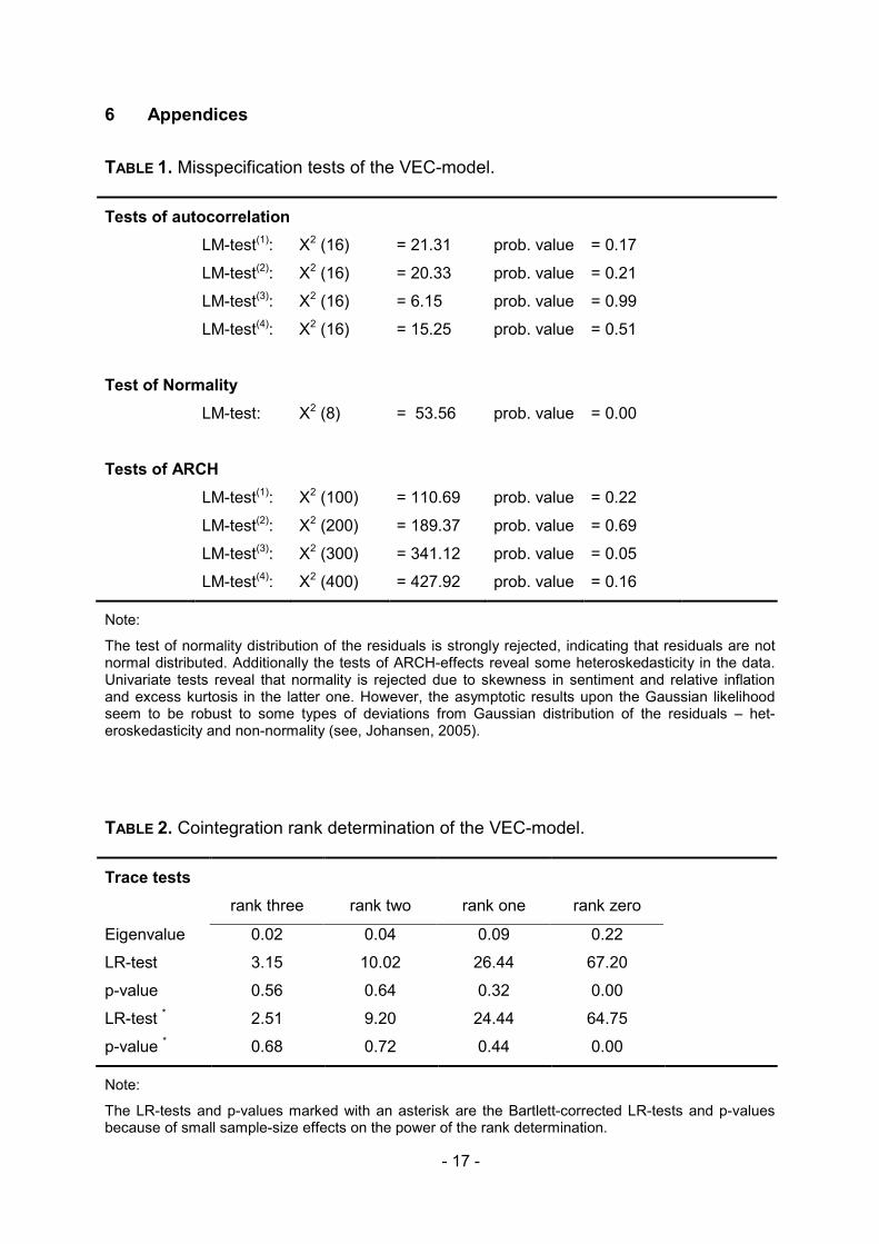
In Table 1 we picture the results of residual tests in order to check the quality

of the model specification. Multivariate LM-tests neither show autocorrelation up to

the fourth order, nor first or second order autoregressive heteroskedasticity. On the

other hand the residuals do not seem to follow a normal distribution very much, but

since the asymptotic results are robust to heteroskedasticity and non-normality, this

should not contradict subsequent inference results seriously as long as the residuals

are i.i.d. (see Johansen, 2005). Identifying the rank of the cointegrated VAR model

we run trace tests, see therefore the results in Table 2. It figures out, that our model

underlies one long-term relation, since a higher-order LR-test could not reject the null

hypothesis of one less existing unit root in the data.

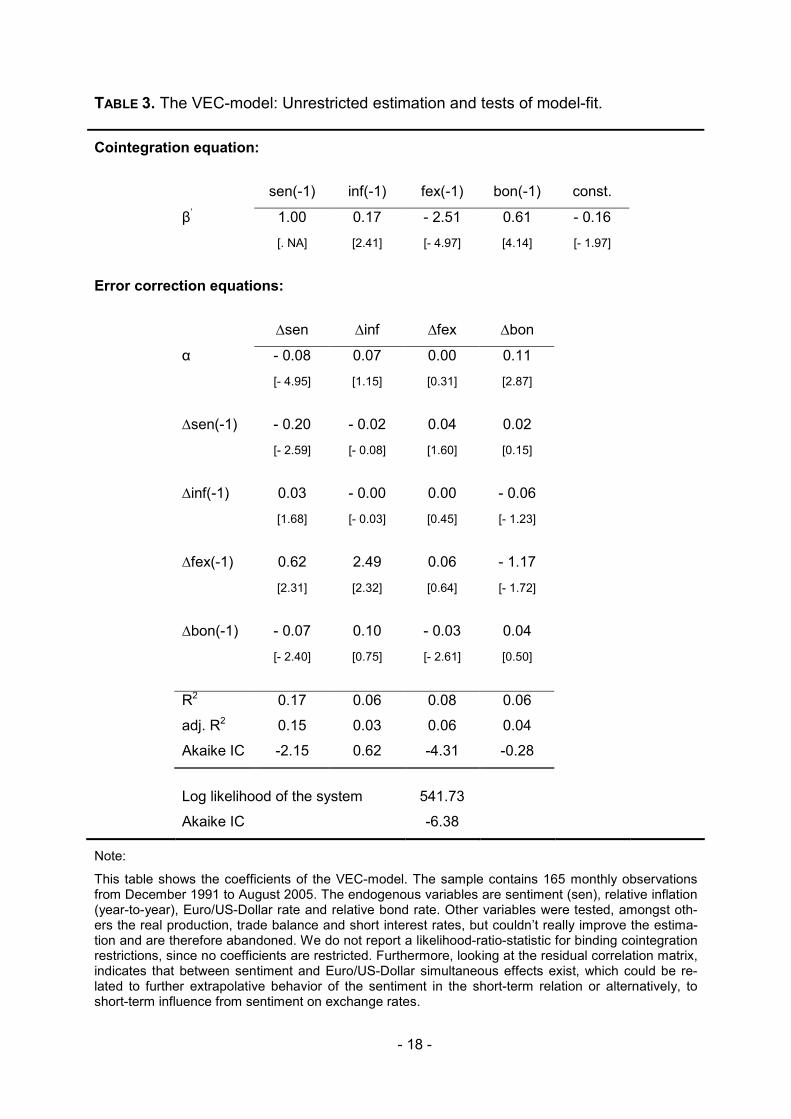
Table 3 presents the results of the vector error-correction model. Regarding

the long-term relation and setting the sentiment’s beta-coefficient to one, it turns out,

that all variables have influence on the sentiment. The relative inflation and bond rate

affect the sentiment positively, which we associate with underlying inflation expecta-

1 We did not find clear evidence of stationarity using the Augmented Dickey Fuller test as well

as the Phillips-Perron test.

- 6 -

tions. The exchange rate stands in a negatively relation to the sentiment and points

to mean-reversion behavior, which corresponds well with former research on expec-

tations data and the idea of the validity of purchasing power parity (in the following

PPP) in the long run. Turning to the short-term dynamics now, we see that next to the

sentiment only bond rates show statistically significant error correction. Then again,

the magnitudes of corresponding alpha-coefficients seem rather small; consequently

the economical significance should be put into question. Furthermore, pulling up the

short-term coefficients from lagged sentiment dynamics, we have to confess, that

sentiment has no impact in the short-run on any of the other variables. Sentiment is

in the short-run positively affected by itself and by the relative bond rate. Further, we

find a negative influence on sentiment from the Euro/US-Dollar, contrary to the

steady-state relation. Putting the contrarian relations between sentiment and bond

rates together, it seems that another type of uncovered interest parity upon bond

rates retains for the sentiment in the long-run. In lieu of the short-run dynamics,

higher interests are followed by expected currency appreciations. However, while the

sentiment shows some kind of extrapolative behavior in the short-run, mean-

reversion dominates the long-run relation with the exchange rate.

So far, our results seem to match prior findings from the analysis of long-term

expectations in such that our sentiment is subject to mean-reversion as well. Addi-

tionally, interest rates influence the sentiment in two different ways, depending on the

time-relation. Hence, because the economical significance of our findings seems to

be questioned, we will tighten these results in the next chapter, where we analyze the

relation between the sentiment, a term of exchange rate mean-reversion and the

bond difference. Considering the latest findings in research of PPP, it shows that this

theory holds - if of any - the long-term, especially if deviations from PPP are big (see

inter alia Kilian and Taylor, 2003). Moreover and as already mentioned in chapter

two, the majority of the survey participants underlying our sentiment use fundamental

information in doing exchange rate analysis. Additionally the positive influence of

bond rates and inflation in long-run point to the importance of inflation expectations,

hence the introduction of a regressive expectation term seems to be reasonable.1

1 For details of our proceeding according to the regressive term, follow the notes of Table 4.

- 7 -

3.2 A threshold cointegrated VAR model

Following up our last findings, we now focus our analysis on the possibility of

threshold effects. So far our results indicate the existence of one long-term relation

upon sentiment. However, the error-corrections don’t appeal to be economically

strong. A reason for this weak evidence could be connected to non-linearity in the

data due to apparent regimes. Specifically to our analysis, we would expect error-

correction depending on the magnitude of fundamental disequilibrium. We have to be

aware, that if more than one long-term relation exists, the results would not be reli-

able. Nevertheless the linear analysis did not show any sign of another valid cointe-

gration relation. In the detected relation, sentiment error-corrects statistically stronger

than any other variable. Since the detected cointegration relation show inter alia

strong mean reversion, we presume that the power of the long-term forces underlying

the sentiment depends on misbalances in respect to either PPP positively. In this

spirit we can draw subsequent analysis on an observable threshold variable and

choose a threshold model accordingly. We see our following analysis very close in

line to Taylor and Peel (2003), Kilian and Taylor (2003) and Sarno and Valente

(2006), who use threshold models to analyze mean reversion in exchange rates.

Whereas Taylor and Peel define exchange rate equilibriums upon a monetary model,

Kilian and Taylor use the PPP concept and so do Sarno and Valente. What all these

elaborations have in common is that exchange rates show mean reversion towards

fundamentals in an extreme regime, where deviations from equilibrium are rather big.

However, in the other regime exchange rates prove to be close to corresponding

fundamentals; hence they show random walk behaviour. However, to model the re-

gimes depending on the magnitudes of exchange rate exuberance, the former two

set an (exponential) smooth threshold autoregressive model (ESTAR), whereas

Sarno and Valente built their analysis upon a Markov switching vector error-

correction model (MS-VECM).

The specific model, on which we built up our analysis, stems from Hansen and

Seo (2002) and features the integration of cointegration analysis. In contrast to simi-

lar methods (for instance Balke and Fomby, 1997), the model’s estimates and tests

are multivariate. The short-term and cointegration coefficients as well as the thresh-

old are jointly estimated via maximum likelihood based upon a specific grid search

- 8 -

algorithm.1 In contrast to Hansen and Seo we handle a three-regime model. To hold

the model tractable, we assume symmetric thresholds, which enable us to concen-

trate on a system with two regimes. Consequently, the threshold variable, z, has to

be measured in absolute terms and determines together with the threshold, γ, the

current regime. We allow also constants in the cointegration space but not in the

short-term dynamics, as we did in the previous analysis. Our model arises as follows:

ε+⋅++⋅+⋅

ε+⋅++⋅+⋅=

−−−

−−−

tktktt

tktktt

txxx

xxxx

∆∆∆∆ΓΓΓΓ∆∆∆∆ΓΓΓΓΠΠΠΠ

∆∆∆∆ΓΓΓΓ∆∆∆∆ΓΓΓΓΠΠΠΠ∆∆∆∆

)2(1

)2(11

)2(

)1(1

)1(11

)1(

L

L

if

if

γ>

γ≤

z

z (3)

with ),0(~ ΣΣΣΣpt Nε and Tt ,...,1= (4)

Since the parameterization of the threshold model is yet unknown, we have to

rely on the linear model in our null hypothesis. Nevertheless the asymptotic distribu-

tion of the appropriate LM test, in order to check the validity of the threshold model,

figures out to be intractable again. To run inference analysis anyhow, Hansen and

Seo suggest two alternative LM-tests via bootstrap techniques, which in contrast pro-

vide asymptotical distributions. The fixed regressor bootstrap, upon which we will

base our threshold test, fixes in contrast to conventional bootstrap technique next to

estimated coefficients and corresponding residuals under the null hypothesis, the

model variable series as well as estimated error-corrections. Modifying the residuals

by adding i.i.d.-innovations of a standard normal distribution, one regress them on

the model variables – once for the whole sample and another time for the split sam-

ples upon the threshold. Using the latter coefficient matrixes and modified residuals

from the former unseparated regression make possible to calculate Eicker-White co-

variance matrix estimators. This in turn enables to calculate a LM-like statistic. Re-

peating these steps numerous times, delivers a simulated distribution of the test sta-

tistic and hence appropriate critical values finally. The alternative procedure is closer

to standard bootstrapping. Here residuals are presumed being i.i.d., but without tak-

1 Confidence intervals for the cointegration parameters (β) are evenly spaced around their linear

estimates and the grid search examines all combinations of β and threshold (γ), which meet the mini-

mum fraction for a regime (trimming parameter).

- 9 -

ing control of potential violations like heteroskedasticity, which has been revealed in

our previous analysis.1

According to our linear estimation in the previous subchapter, we assume one

lag in the VAR-setting. Depending upon the threshold value all coefficients are al-

lowed to differ. We set the trimming parameter rather conservative at 0.20 due to our

small sample size. Setting the grid sizes for the cointegration coefficients to 100 and

to 300 for the threshold variable, we run 1000 bootstraps. Furthermore we choose

the Eicker-White covariance matrix to correct potential heteroskedasticity in the re-

siduals. Special attention arises from the choice of the threshold variable. In contrast

to Hansen and Seo we do not focus to choose the error-correction variable as the

threshold variable, but rather the regressive term in absolute values.

However, the estimations differ depending on the implemented threshold vari-

able. Choosing the error-corrections as the threshold, resulting estimations become

odd. Particularly, the error-corrections in the sentiment do not differ between the re-

gimes and the existence of a nonlinear threshold model is strongly rejected.2 In con-

trast the results with the regressive term as the threshold variable turn out being very

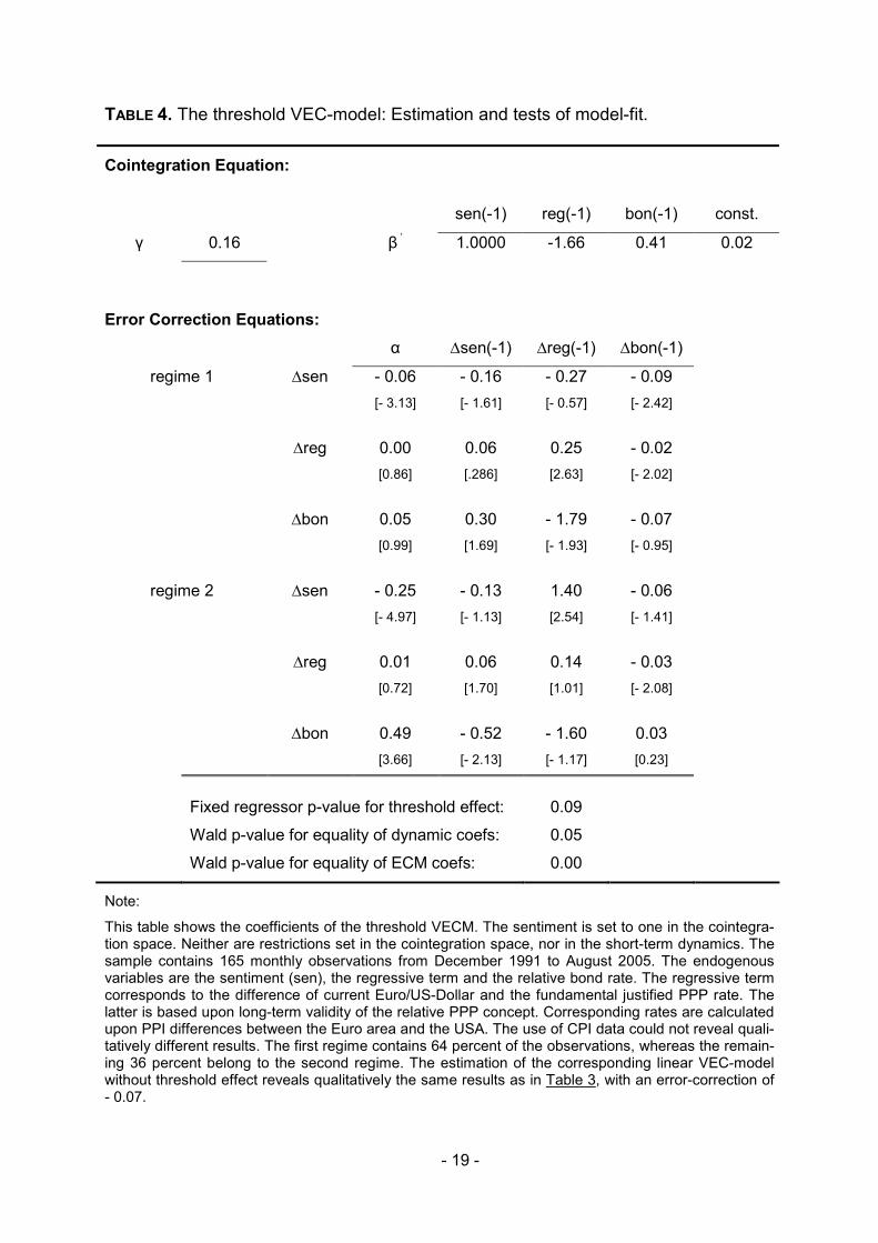
much in line with our prior belief. The results are shown in Table 4. We denote a

threshold of approx. 0.16. This constitutes the first regime, if the exchange rate is

close to the PPP-rate in a band of 20 percent. Hence, the second regime holds, if the

exchange rate is above the band, being far away from PPP. Therefore we define the

first regime as the “tranquil” regime, whereas the second represent the “extreme” re-

gime. As assumed, error-correction in the sentiment increases, when leaving the

tranquil regime and turning into the extreme regime (from 0.06 to 0.24). Additionally,

being in the tranquil regime, sentiment is influenced positively by interest rates in the

short-term but vice versa in the extreme regime. Furthermore, short-term influence by

the regressive term on the sentiment takes place in the extreme regime, which we

assume being connected with existing trends in this regime.

All in all, it figures out, that expectations anticipate stronger mean reversion in

situations, where fundamental discrepancy between exchange rates and PPP-rates

1 The fixed regressor bootstrap is robust to heteroskedasticity (see Hansen and Seo, 2002).

2 To conserve space, we skip corresponding results.

- 10 -

are the biggest. Only in this regime we evaluate the long-term forces towards PPP

underlying the sentiment being both statistically and economically significant.1

4 Forward-looking attributes of sentiment

Finally we examine the sentiment in respect to its ability to forecasting ex-

change rates. Since we figured out, that sentiment is better described by fundamen-

tals in extreme circumstances and in case sentiment contains valuable forecasting

information, it would be of high interest knowing in which time horizon.

For this purpose we will pursue two approaches. First, we will look at some

standard calculations, such as the mean error (ME) or the root mean square error

(RMSE). Second, we will investigate the contribution of sentiment in explaining fol-

lowing average returns in Euro/US-Dollar. Doing so, we will use subsequent time pe-

riods from one month up to 60 months.

4.1 Accuracy of sentiment forecasts

To throw light on the forecasting property of the sentiment and respectively to

provide some standard information for comparisons with other forecasts, we investi-

gate common calculations in respect to the quality of the sentiment forecasts. As

most of the standard analysis is based upon point forecasts, we have to transform

the sentiment data. One appropriate possibility to accomplish is to quantify aggre-

gated expectations via the Carlson and Parkin approach (1975). Applying this

method we get point forecasts which enable us to run adequate accuracy tests.

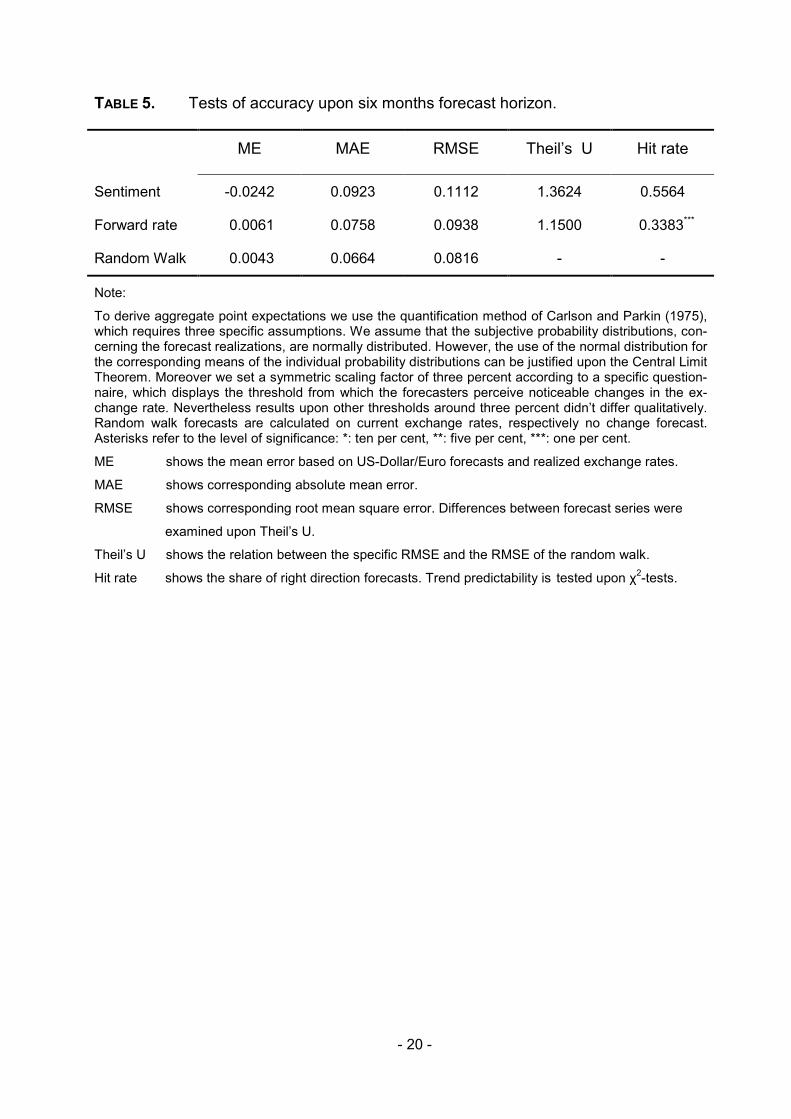
Table 5 represents the corresponding results in congruency with the surveyed

six months forecast horizon. Furthermore and for comparative purposes, calculations

are run for forecasts upon the forward rate as well as the random walk. Obviously

aggregated expectations perform worse than competing forecast series in all tests

except for the hit rate. The mean error, mean absolute error and the root mean

square error of the expectations are in all cases bigger than accordant numbers from

the forward rate and the random walk. Direct comparisons between expectations as

1 Note that we do not deduce upon our analysis exchange rate behaviour towards PPP by itself.

- 11 -

well as forward rates with the random walk reveals, that the latter performs the best.

However, consulting the hit rate, which displays the share of correct trend forecasts,

shows undoubtedly advantages towards expectations. Trend forecasts upon expec-

tations reveal a 55 percent hit rate, whereas forward rates prove correctness in only

30 percent of the cases.1

Even though we assume six months expectations, due to the design of the sur-

vey, the short-term orientation of financial markets indicates by itself that our senti-

ment underlies rather long-term considerations. Alternatively, if expectations are bi-

ased upon strong fundamental beliefs, which would be associated with a form of

wishful thinking similar to Ito’s findings (1990), forecasters anticipate too much mean

reversion according to what fundamentals actually speak (1990).2

4.2 Sentiment in a long-horizon setting

In this chapter we build up long-term regressions to follow the idea of fairly long-

term sentiment. We target the simulation-analysis of Brown and Cliff (2005) who in-

vestigate sentiment on US equity index using bootstrap technique.

ktt

kt

kkkt Sr ε+⋅β+⋅+α= z'ΘΘΘΘ (5)

We regress k-period average returns of the Euro/US-Dollar, rtk, on a vector of

control variables, zt, in which we put change of differences in domestic vs. foreign

short term interest rate, term structure, inflation rate, equity index, production index,

trade balance and the sentiment, St. We consider a large set of additional regressors,

since we are in need of control for potential explanatory variables of exchange rate

returns as well as the sentiment. Given that we built up a rather long-term analysis,

we concentrate on variables, which are known of having some explanatory power in

the long run on exchange rates.

The difficulty we are confronted with is twofold. On the one hand, we have to

overcome an overlapping problem (see Hansen and Hodrick, 1980). Since we calcu-

1 Remember the random walk forecasts no change; hence, the benchmark is set at 50 percent.

2 See Menkhoff et al. (2006), who alternatively consider rational forecasters, since the market

environment is too short-term orientated, given fundamental circumstances.

- 12 -

late average returns of sequential periods, we obtain a moving average process of

the dimension of the specific period in the error term, εtk. Basically one overcomes

this issue using Newey-West standard errors, but due to our relatively small sample

size, this correction has small power (see inter alia Hodrick, 1992). Another issue

which must be taken into account arises from persistent behavior of some of the re-

gressors, which constitute a potential source of bias in consecutive estimates even

though corresponding regressors are preparatory (see Stambaugh, 1999). Following

Brown and Cliff (2005), we run a bootstrap with 10,000 simulations in order to derive

more accurate estimate results from simulated distributions, upon which our following

inference analysis is based.

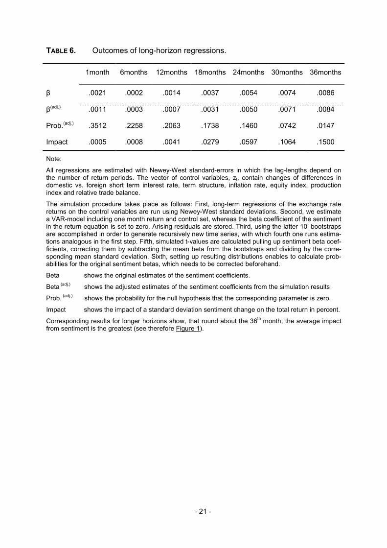
The outcomes, presented in Table 6, reveal an interesting pattern. In the short-

run, we cannot detect any prediction ability of the sentiment. Not until approx. two

and a half years, sentiment shows contribution in order to predict subsequent returns

in the Euro/US-Dollar. Strikingly, from month 32 upwards, the corrected beta coeffi-

cient from the sentiment variable turns out being significant. Getting an idea about

the magnitude of the influence on returns, we apply to a one standard deviation of

the sentiment and calculate potential impacts on subsequent total Euro/US-Dollar

returns. Glancing at two examples, the total impact of sentiment on following six

month returns yields on average 0.08 percent, whereas corresponding impact on 36

months returns ads up to 15 percent.

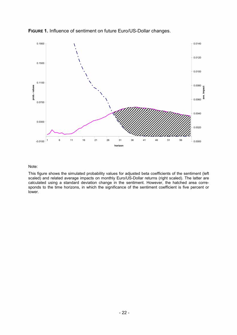
It seems that sentiment reveal valuable information in order to predict longer-

term returns. This finding is in line with Kilian and Taylor (2003), whose exchange

rate predictions from an ESTAR model based upon PPP did not start to value before

two to three years. On the other hand our sentiment obviously does not serve well as

a contrarian indicator in the short-run. Figure 1 merges these findings, where the

hatched area is associated to the periods, in which the sentiment contains additional

information in order to predict subsequent exchange rate returns on a minimum al-

pha-error of five percent.

5 Conclusions

Our results match prior research on exchange rate expectations, whereas a

form of mean-reversion characterizes long-term expectations and therefore our sen-

- 13 -

timent. Additionally, interest rates influence the sentiment, but in two different ways

depending on the time-relation. Nevertheless the sentiment contains stronger mean

reversion in situations, where fundamental discrepancy between exchange rates and

PPP-rates are the biggest. Only in this regime we evaluate the long-term forces to-

wards PPP underlying the sentiment being both statistically and economically signifi-

cant. Return to mind; the majority of the survey participants underlying our sentiment

use fundamental information in doing exchange rate analysis. Note, that we do not

deduce from our analysis exchange rate behaviour towards PPP by itself.

Considering the short-run focus of exchange rate markets, six months expec-

tations horizon appears being rather long-term. Hence, the sentiment shows long-

term anchorage. Alternatively, the sentiment is strongly biased towards (longer-term)

fundamental concepts. This would be associated with a form of “wishful thinking”

similar to Ito’s finding (1990) but in the way, that forecasters anticipate too much be-

lief in mean reversion according to what the fundamentals speak.

Putting all this together, sentiment reveals some valuable information in respect

of very long-term exchange rate returns. On the other hand it does not contain any

valuable information concerning shorter-term exchange rate returns. This finding is in

line with Kilian and Taylor (2003), where the exchange rate predictions of an ESTAR

model based upon the PPP-concept do not start to value earlier than two to three

years.

- 14 -

References

Bacchetta, Philippe and Eric van Wincoop (2004), A scapegoat model of exchange-

rate fluctuations, American Economic Review, 94(2): 114-18.

Baker, Malcolm and Jeffrey Wurgler (2005), Investor sentiment and the cross-section

of stock returns, Journal of Finance, forthcoming.

Balke, N.S. and T.B. Fomby (1997), Threshold cointegration, International Economic

Review, 48: 627-45.

Barberis, Nicholas, Andrei Shleifer and Robert Vishny (1998), A model of investor

sentiment, Journal of Financial Economics, 49: 307-43.

Brown, Gregory W. and Michael T. Cliff (2005), Investor sentiment and asset valua-

tion, Journal of Business, 78(2): 405-40.

Carlson, John A. and Michael Parkin (1975), Inflation Expectations, Economica, 42:

123-38.

DeGrauwe, Paul and Marianne Grimaldi (2006), Exchange rate puzzles: A tale of

switching attractors, European Review, 50: 1-33.

DeLong, J. Bradford, Andrei Shleifer, Lawrence H. Summer and Robert J. Waldmann

(1990), Noise trader risk in financial markets, Journal of Political Economy,

98(4): 703-38.

Dominguez, Kathryn M. (1986), Are foreign exchange forecasts rational? New evi-

dence from survey data, Economics Letters, 21: 277-281.

Frankel, Jeffrey A. and Kenneth A. Froot (1987a), Using survey data to test standard

propositions regarding exchange rate expectations, American Economic Re-

view, 77(1): 133-53.

Frankel, Jeffrey A. and Kenneth A. Froot (1990), Chartists, fundamentalists, and trad-

ing in the foreign exchange market, American Economic Review, 80(2): 181-

85.

- 15 -

Frydman, Roman and Michael D. Goldberg (2003), Imperfect knowledge expecta-

tions, uncertainty adjusted UIP and exchange rate dynamics, in: Aghion, P.,

Frydman, R. Stiglitz, J. and M. Woodford (eds.), Knowledge, information and

expectations in modern macroeconomics: In honor of Edmund S. Phelps,

Princeton, NJ: Princeton University Press.

Hansen, Lars P. and Robert J. Hodrick (1980), Foreign Exchange Rates as Optimal

Predictors of Future Spot Rates: An Econometric Analysis, Journal of Politi-

cal Economy, 88: 829-53.

Hansen, Bruce E. and Byeongseon Seo (2002), Testing for two-regime threshold

cointegration in vector error-correction models, Journal of Econometrics,

110: 293-318.

Hodrick, Robert J. (1992), Dividend yields and expected stock returns: Alternative

procedures for inference and measurement, Review of Financial Studies,

5:357-86.

Ito, Takatoshi (1990), Foreign Exchange Rate Expectations: Micro Survey Data,

American Economic Review, 80:3, 434-49.

Johansen, Sören (2005), Cointegration: A survey, in: T.C. Mills and K. Patterson

(eds.), Palgrave Handbook of Econometrics: Vol. 1, Econometric Theory,

Basingstoke, Palgrave Macmillan.

Kilian, Lutz and Mark P. Taylor (2003), Why is it so difficult to beat the random walk

forecast of exchange rates?, Journal of International Economics, 60: 85-107.

MacDonald, Ronald (2000), Expectations formation and risk in three financial mar-

kets: Surveying what the surveys say, Journal of Economic Surveys, 14(1): 69-

100.

Menkhoff, Lukas, Rafael R. Rebitzky and Michael Schröder (2006), Do Dollar fore-

casters believe too much in PPP, Applied Economics, forthcoming.

Qiu, Lily and Ivo Welch (2004), Investment sentiment measures, NBER Working Pa-

per, September, Nr. 10794.

Sarno, Lucio (2005), Viewpoint: Towards a solution to the puzzles in exchange rate

economics: Where do we stand?, Canadian Journal of Economics 38(3): 673-

708.

- 16 -

Sarno, Lucio and Giorgio Valente (2006), Deviations from Purchasing Power Parity

under different exchange rate regimes: Do they revert and, if so, how?, Journal

of Banking and Finance, forthcoming.

Shiller, Robert J. (1990), Speculative prices and popular models, Journal of Eco-

nomic Perspectives, 4(2): 55-65.

Stambaugh, Robert F. (1999), Predictive regressions, Journal of Financial Econom-

ics, 54: 375-421.

Taylor, Mark P. and David A. Peel (2003), Nonlinear adjustment, long-run equilibrium

and exchange rate fundamentals, Journal of International Economics, 60: 85-

107.

ZEW Centre for European Economic Research (2004), Financial Market Report,

13:2.

- 17 -

6 Appendices

TABLE 1. Misspecification tests of the VEC-model.

Tests of autocorrelation

LM-test(1): Χ2 (16) = 21.31 prob. value = 0.17

LM-test(2): Χ2 (16) = 20.33 prob. value = 0.21

LM-test(3): Χ2 (16) = 6.15 prob. value = 0.99

LM-test(4): Χ2 (16) = 15.25 prob. value = 0.51

Test of Normality

LM-test: Χ2 (8) = 53.56 prob. value = 0.00

Tests of ARCH

LM-test(1): Χ2 (100) = 110.69 prob. value = 0.22

LM-test(2): Χ2 (200) = 189.37 prob. value = 0.69

LM-test(3): Χ2 (300) = 341.12 prob. value = 0.05

LM-test(4): Χ2 (400) = 427.92 prob. value = 0.16

Note:

The test of normality distribution of the residuals is strongly rejected, indicating that residuals are not normal distributed. Additionally the tests of ARCH-effects reveal some heteroskedasticity in the data. Univariate tests reveal that normality is rejected due to skewness in sentiment and relative inflation and excess kurtosis in the latter one. However, the asymptotic results upon the Gaussian likelihood seem to be robust to some types of deviations from Gaussian distribution of the residuals – het-eroskedasticity and non-normality (see, Johansen, 2005).

TABLE 2. Cointegration rank determination of the VEC-model.

Trace tests

rank three rank two rank one rank zero

Eigenvalue 0.02 0.04 0.09 0.22

LR-test 3.15 10.02 26.44 67.20

p-value 0.56 0.64 0.32 0.00

LR-test * 2.51 9.20 24.44 64.75

p-value * 0.68 0.72 0.44 0.00

Note:

The LR-tests and p-values marked with an asterisk are the Bartlett-corrected LR-tests and p-values because of small sample-size effects on the power of the rank determination.

- 18 -

TABLE 3. The VEC-model: Unrestricted estimation and tests of model-fit.

Cointegration equation:

sen(-1) inf(-1) fex(-1) bon(-1) const.

β’ 1.00 0.17 - 2.51 0.61 - 0.16

[. NA] [2.41] [- 4.97] [4.14] [- 1.97]

Error correction equations:

∆sen ∆inf ∆fex ∆bon

α - 0.08 0.07 0.00 0.11

[- 4.95] [1.15] [0.31] [2.87]

∆sen(-1) - 0.20 - 0.02 0.04 0.02

[- 2.59] [- 0.08] [1.60] [0.15]

∆inf(-1) 0.03 - 0.00 0.00 - 0.06

[1.68] [- 0.03] [0.45] [- 1.23]

∆fex(-1) 0.62 2.49 0.06 - 1.17

[2.31] [2.32] [0.64] [- 1.72]

∆bon(-1) - 0.07 0.10 - 0.03 0.04

[- 2.40] [0.75] [- 2.61] [0.50]

R2 0.17 0.06 0.08 0.06

adj. R2 0.15 0.03 0.06 0.04

Akaike IC -2.15 0.62 -4.31 -0.28

Log likelihood of the system 541.73

Akaike IC -6.38

Note:

This table shows the coefficients of the VEC-model. The sample contains 165 monthly observations from December 1991 to August 2005. The endogenous variables are sentiment (sen), relative inflation (year-to-year), Euro/US-Dollar rate and relative bond rate. Other variables were tested, amongst oth-ers the real production, trade balance and short interest rates, but couldn’t really improve the estima-tion and are therefore abandoned. We do not report a likelihood-ratio-statistic for binding cointegration restrictions, since no coefficients are restricted. Furthermore, looking at the residual correlation matrix, indicates that between sentiment and Euro/US-Dollar simultaneous effects exist, which could be re-lated to further extrapolative behavior of the sentiment in the short-term relation or alternatively, to short-term influence from sentiment on exchange rates.

- 19 -

TABLE 4. The threshold VEC-model: Estimation and tests of model-fit.

Cointegration Equation:

sen(-1) reg(-1) bon(-1) const.

γ 0.16 β ’ 1.0000 -1.66 0.41 0.02

Error Correction Equations:

α ∆sen(-1) ∆reg(-1) ∆bon(-1)

regime 1 ∆sen - 0.06 - 0.16 - 0.27 - 0.09

[- 3.13] [- 1.61] [- 0.57] [- 2.42]

∆reg 0.00 0.06 0.25 - 0.02

[0.86] [.286] [2.63] [- 2.02]

∆bon 0.05 0.30 - 1.79 - 0.07

[0.99] [1.69] [- 1.93] [- 0.95]

regime 2 ∆sen - 0.25 - 0.13 1.40 - 0.06

[- 4.97] [- 1.13] [2.54] [- 1.41]

∆reg 0.01 0.06 0.14 - 0.03

[0.72] [1.70] [1.01] [- 2.08]

∆bon 0.49 - 0.52 - 1.60 0.03

[3.66] [- 2.13] [- 1.17] [0.23]

Fixed regressor p-value for threshold effect: 0.09

Wald p-value for equality of dynamic coefs: 0.05

Wald p-value for equality of ECM coefs: 0.00

Note:

This table shows the coefficients of the threshold VECM. The sentiment is set to one in the cointegra-tion space. Neither are restrictions set in the cointegration space, nor in the short-term dynamics. The sample contains 165 monthly observations from December 1991 to August 2005. The endogenous variables are the sentiment (sen), the regressive term and the relative bond rate. The regressive term corresponds to the difference of current Euro/US-Dollar and the fundamental justified PPP rate. The latter is based upon long-term validity of the relative PPP concept. Corresponding rates are calculated upon PPI differences between the Euro area and the USA. The use of CPI data could not reveal quali-tatively different results. The first regime contains 64 percent of the observations, whereas the remain-ing 36 percent belong to the second regime. The estimation of the corresponding linear VEC-model without threshold effect reveals qualitatively the same results as in Table 3, with an error-correction of - 0.07.

- 20 -

TABLE 5. Tests of accuracy upon six months forecast horizon.

ME MAE RMSE Theil’s U Hit rate

Sentiment -0.0242 0.0923 0.1112 1.3624 0.5564

Forward rate 0.0061 0.0758 0.0938 1.1500 0.3383***

Random Walk 0.0043 0.0664 0.0816 - -

Note:

To derive aggregate point expectations we use the quantification method of Carlson and Parkin (1975), which requires three specific assumptions. We assume that the subjective probability distributions, con-cerning the forecast realizations, are normally distributed. However, the use of the normal distribution for the corresponding means of the individual probability distributions can be justified upon the Central Limit Theorem. Moreover we set a symmetric scaling factor of three percent according to a specific question-naire, which displays the threshold from which the forecasters perceive noticeable changes in the ex-change rate. Nevertheless results upon other thresholds around three percent didn’t differ qualitatively. Random walk forecasts are calculated on current exchange rates, respectively no change forecast. Asterisks refer to the level of significance: *: ten per cent, **: five per cent, ***: one per cent.

ME shows the mean error based on US-Dollar/Euro forecasts and realized exchange rates.

MAE shows corresponding absolute mean error.

RMSE shows corresponding root mean square error. Differences between forecast series were

examined upon Theil’s U.

Theil’s U shows the relation between the specific RMSE and the RMSE of the random walk.

Hit rate shows the share of right direction forecasts. Trend predictability is tested upon χ2-tests.

- 21 -

TABLE 6. Outcomes of long-horizon regressions.

1month 6months 12months 18months 24months 30months 36months

β .0021 .0002 .0014 .0037 .0054 .0074 .0086

β(adj.) .0011 .0003 .0007 .0031 .0050 .0071 .0084

Prob.(adj.) .3512 .2258 .2063 .1738 .1460 .0742 .0147

Impact .0005 .0008 .0041 .0279 .0597 .1064 .1500

Note:

All regressions are estimated with Newey-West standard-errors in which the lag-lengths depend on the number of return periods. The vector of control variables, zt, contain changes of differences in domestic vs. foreign short term interest rate, term structure, inflation rate, equity index, production index and relative trade balance.

The simulation procedure takes place as follows: First, long-term regressions of the exchange rate returns on the control variables are run using Newey-West standard deviations. Second, we estimate a VAR-model including one month return and control set, whereas the beta coefficient of the sentiment in the return equation is set to zero. Arising residuals are stored. Third, using the latter 10’ bootstraps are accomplished in order to generate recursively new time series, with which fourth one runs estima-tions analogous in the first step. Fifth, simulated t-values are calculated pulling up sentiment beta coef-ficients, correcting them by subtracting the mean beta from the bootstraps and dividing by the corre-sponding mean standard deviation. Sixth, setting up resulting distributions enables to calculate prob-abilities for the original sentiment betas, which needs to be corrected beforehand.

Beta shows the original estimates of the sentiment coefficients.

Beta (adj.)

shows the adjusted estimates of the sentiment coefficients from the simulation results

Prob. (adj.)

shows the probability for the null hypothesis that the corresponding parameter is zero.

Impact shows the impact of a standard deviation sentiment change on the total return in percent.

Corresponding results for longer horizons show, that round about the 36th month, the average impact

from sentiment is the greatest (see therefore Figure 1).

- 22 -

FIGURE 1. Influence of sentiment on future Euro/US-Dollar changes.

-0.0100

0.0300

0.0700

0.1100

0.1500

0.1900

1 6 11 16 21 26 31 36 41 46 51 56

horizon

prob.- valuee

0.0000

0.0020

0.0040

0.0060

0.0080

0.0100

0.0120

0.0140

ave. impact

Note:

This figure shows the simulated probability values for adjusted beta coefficients of the sentiment (left scaled) and related average impacts on monthly Euro/US-Dollar returns (right scaled). The latter are calculated using a standard deviation change in the sentiment. However, the hatched area corre-sponds to the time horizons, in which the significance of the sentiment coefficient is five percent or lower.