Sentiment Analysis on Twitter with Stock Price and Significant

Keyword Correlation

Linhao Zhang

Department of Computer Science, The University of Texas at Austin

(Dated: April 16, 2013)

Abstract

Though uninteresting individually, Twitter messages, or tweets, can provide an accurate reflec-

tion of public sentiment on when taken in aggregation. In this paper, we primarily examine the

effectiveness of various machine learning techniques on providing a positive or negative sentiment

on a tweet corpus. Additionally, we apply extracted twitter sentiment to accomplish two tasks.

We first look for a correlation between twitter sentiment and stock prices. Secondly, we determine

which words in tweets correlate to changes in stock prices by doing a post analysis of price change

and tweets. We accomplish this by mining tweets using Twitter’s search API and subsequently

processing them for analysis. For the task of determining sentiment, we test the effectiveness

of three machine learning techniques: Naive Bayes classification, Maximum Entropy classification,

and Support Vector Machines. We discover that SVMs give the highest consistent accuracy through

cross validation, but not by much. Additionally, we discuss various approaches in training these

classifiers. We then apply our findings to on an intra-day market scale to find that there is very

little direct correlation between stock prices and tweet sentiment on specifically an intra-day scale.

Next, we improve on the keyword search approach by reverse correlating stock prices to individual

words in tweets, finding, reasonably, that certain keywords are more correlated with changes in

stock prices. Lastly, we discuss various challenges posed by looking at twitter for performing stock

predictions.

1

I. INTRODUCTION

Throughout a day, large amounts of text are transmitted online through a variety of social

media channels. Within these texts, valuable information about virtually every topic exists.

Through Twitter alone, over 400 million tweets are sent per day. If each has a maximum of

140 characters, that’s over 56 billion characters generated per day, just on Twitter. Though

each tweet may not seem extremely valuable, it has been argued that aggregations of large

amounts of tweets can provide valuable insight about public mood and sentiment on certain

topics [10].

Recently, an interesting problem in Computer Science has been to effectively make sense

of information presented on the web. This involves separate tasks of mining data from web-

sites, storing it, and running data analysis on gigantic amounts of text to extract relevant

information. With the growth of social network and microblogging sites, this problem be-

comes even more relevant. In the case of Twitter, it involves collecting a large number of

tweets and analyzing them on a large scale to gauge the Twittersphere’s opinion on a topic.

The applications of this information from a financial standpoint are numerous. Gauging

the public’s sentiment by retrieving online information on the market can be valuable in

creating trading strategies. This is not technical analysis of stocks, but rather fundamental

analysis through data mining. There are many factors that are involved in prediction or

analyzing the movement of stock prices, and public sentiment is arguably included.

In this paper, we take a look at three machine learning techniques that are commonly used

for classification, and examine their effectiveness on a Twitter corpus. Also, we investigate

the extent to which Twitter sentiment is correlated to stock prices on an intra-day scale, and

at the same time research which individual words from tweets are correlated with changes

in stock prices. Of course, true stock price correlations involve many more factors, but we

will just look at the correlation between Twitter sentiment and stock price, merely as an

interesting application of sentiment analysis.

II. RELATED WORK

The proliferation of online documents and user generated texts has led to a recent growth

in research in the area of sentiment analysis and its relationship to financial markets. A

2

broad overview of some of the machine learning techniques used in sentiment classification

is provided in [15]. There, they investigate methods in determining whether movie reviews

are positive or negative and examine some challenges in sentiment mining. They provide

an overview of Naive Bayes, Maximum Entropy, and Support Vector Machine classification

techniques in the movie review domain.

[14] discusses the use of Twitter specifically as a corpus for sentiment analysis. They

discuss the methods of tweet gathering and processing. The authors use specific emoticons

to form a training set for sentiment classification, a technique that greatly reduces manual

tweet tagging. Their training set was split into positive and negative samples based on

happy and sad emoticons. Additionally, they analyze a few accuracy improvement methods.

Similarly, [3] presents a discussion of streaming Tweet mining and sentiment extraction,

while furthering the discussion to include opinion mining.

[4] presented one of the first indications that there may be a correlation between Twitter

sentiment and the stock market. In their work, a sentiment score is correlated with the DJIA

and then fed into a neural network to predict market movements. The authors use a mood

tracking tool named OpinionFinder to measure mood in 6 dimensions (Calm, Alert, Sure,

Vital, Kind, and Happy). Then, they correlate the mood time series with DJIA closing values

by using a Self Organizing Fuzzy Neural Network. Using their techniques, they measured

an improvement on DJIA prediction accuracy. After publication, this paper launched much

of the current research in the relationship between twitter and market sentiments.

A few other techniques in the area have been proposed. [6] provides a method in which

tweets are screened for stock symbols, then sentiment is gathered using Nave Bayes over

an existing dataset. Their research continues and is still in the data collection phase. [9]

combines sentiment gathered from news with technical features of stock data. Sentiment

is analyzed using SentiWordNet 3.0 [1], a lexical resource for opinion mining. Instead of

Twitter, they scrape data from Engadget. Multiple kernel learning is run to find the best

coefficients for the different factors in their system for stock prediction. The authors found

that training a model based on more than technical stock indicators improved stock predic-

tion performance.

[11] discusses three methods of sentiment analysis on tweets: document-level, sentence-

level, and aspect-based. They conclude that aspect-based analysis, which tries to recognize

all sentiment within a document and the aspects which they refer to, is the most fine grained

3

approach for the problem. Additionally, they outline various challenges of sentiment analysis

on tweets, some of which we run into as well.

[13] achieves a 75% accurate prediction mechanism using Self Organizing Fuzzy Neural

Networks on Twitter and DJIA feeds. In their research, they created a custom questionnaire

with words to analyze tweets for their sentiment. Their work is similar to [4], with a few

minor modifications.

On a side note, [12] discusses some common problems involved in many of the techniques

presented above. These include, but are not limited to: insufficient data, inaccurate measures

of performance, and inappropriate scaling.

The techniques proposed by these papers provide an interesting overview of sentiment

analysis and how it can relate to the stock market. However, the results seem varied and may

depend on the accuracy of a twitter sentiment classifier, as well as pre-processing and filtering

of tweets, including which tweets to use for analysis. The market and keywords used are

not detailed in most of these papers, which play a heavy role in determining whether or not

the system is effective in stock prediction. In this work, we emulate some of these previous

works to build a sentiment analyzer, but specifically for the Twitter domain. However, in

addition to correlating stock price, we look for correlations in particular words in tweets

that indicate positive and negative market movements after-the-fact.

4

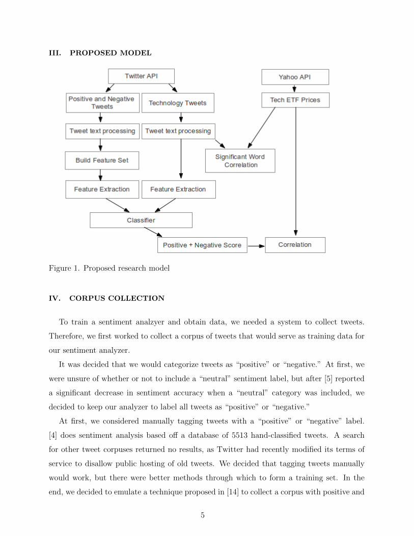
III. PROPOSED MODEL

Figure 1. Proposed research model

IV. CORPUS COLLECTION

To train a sentiment analzyer and obtain data, we needed a system to collect tweets.

Therefore, we first worked to collect a corpus of tweets that would serve as training data for

our sentiment analyzer.

It was decided that we would categorize tweets as “positive” or “negative.” At first, we

were unsure of whether or not to include a “neutral” sentiment label, but after [5] reported

a significant decrease in sentiment accuracy when a “neutral” category was included, we

decided to keep our analyzer to label all tweets as “positive” or “negative.”

At first, we considered manually tagging tweets with a “positive” or “negative” label.

[4] does sentiment analysis based off a database of 5513 hand-classified tweets. A search

for other tweet corpuses returned no results, as Twitter had recently modified its terms of

service to disallow public hosting of old tweets. We decided that tagging tweets manually

would work, but there were better methods through which to form a training set. In the

end, we decided to emulate a technique proposed in [14] to collect a corpus with positive and

5

negative sentiments without any manual effort for classification. To do this, we employed

use of Twitter’s Search API.

A. Twitter Search/Streaming API

For tweet collection, Twitter provides a rather robust API. There are two possible ways

to gather Tweets: the Streaming API or the Search API. The Streaming API allows users to

obtain real-time access to tweets from an input query. The user first requests a connection

to a stream of tweets from the server. Then, the server opens a streaming connection and

tweets are streamed in as they occur, to the user.

However, there are a few limitations of the Streaming API. First, language is not specifi-

able, resulting in a stream that contains Tweets of all languages, including a few non-Latin

based alphabets. Additionally, at the free level, the streamed Tweets are only a small frac-

tion of the actual Tweet body (gardenhose vs. firehose). Initial testing with the streaming

API resulted in a polluted training set as it proved difficult to obtain a pure dataset of

Tweets.

Because of these issues, we decided to go with the Twitter Search API instead. The Search

API is a REST API which allows users to request specific queries of recent tweets. REST, or

Representational State Transfer, simply uses HTTP methods (GET, POST, PUT, DELETE)

to execute different operations. The Search API allows more fine tuning of queries, including

filtering based on language, region, and time. There is a rate limit associated with the query,

but we handle it in the code. For our purposes, the rate limit has not been an issue. To

actually fetch tweets, we continuously send queries to the Search API, with a small delay

to account for the rate limit. The query (shown below) is constructed by stringing separate

keywords together with an “OR” in between. Though this is also not a fully complete result,

it returns a well filtered set of tweets that is useful for our sentiment analyzer.

The request returns a list of JSON objects that contain the tweets and their metadata.

This includes a variety of information, including username, time, location, retweets, and

more. For our purposes, we mainly focus on the time and tweet text.

Both of these APIs require the user have an API key for authentication. Once authen-

ticated, we were able to easily access the API through a python library called Twython- a

simple wrapper for the Twitter API.

6

B. Training Set Collection

Using Twitter’s search API, we formed two separate datasets (collections of Tweets) for

training: “positive” and “negative.” Each dataset was formed programmatically and based

on positive and negative queries on emoticons and keywords:

• Positive sentiment query: “:) OR :-) OR =) OR :D OR <3 OR like OR love”

• Negative sentiment query: “:( OR =( OR hate OR dislike”

The reasoning behind these keywords is straightforward. The tweets that contained these

keywords or emoticons were most likely to be of that corresponding sentiment. This results

in a training set of “positive” and “negative” tweets that was nearly as good as manual

tagging. Another advantage of programmatically mining tweets with prior sentiment is that

we were able to mine many, many more. In all, we gathered over 500,000 tweets of each

sentiment. Unfortunately, I did not have the computational power to train over all the

tweets, but the sample size was definitely increased over merely manually annotating tweets

with a sentiment label.

C. MongoDB Storage

To save our training tweet data, we used MongoDB. MongoDB is a document based

database in which data is stored as JSON-like objects. Naturally, this works well with the

tweet objects returned from the API. Each tweet is simply stored as a record in a collection

in the database. Not all the data is stored, though- only relevant information, including

tweet text and date. Querying the MongoDB database is simple as well- one iterator simply

crawls through an entire collection of tweets during training and classification tasks.

V. TWEET TEXT PROCESSING

The text of each tweet contains many extraneous words that do not contribute

to its sentiment. Many tweets include URLS, tags to other users, or symbols that

have no meaning. To accurately obtain a tweet’s sentiment, we first need to filter the

noise from its original state. To do this, we incorporate a variety of techniques. An

7

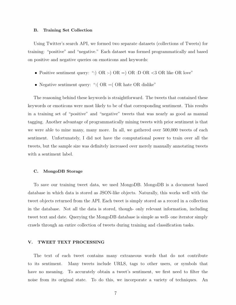
example of common tweet characters and formats can be seen in Table 1. Before pro-

cessing, many of the tweets characters and words merely add noise to our sentiment analysis.

Table 1. Tweet examples

A. Tokenization

The first step involves splitting the text by spaces, forming a list of individual words per

text. This is also called a bag of words. We will later use each word in the tweet as features

to train our classifier.

B. Removing Stopwords

Next, we remove stopwords from the bag of words. Python’s Natural Language Toolkit

library contains a stopword dictionary. To remove the stopwords from each text, we simply

check each word in the bag of words against the dictionary. If a word is a stopword, we filter

it out. The list of stopwords contains articles, some prepositions, and other words that add

no sentiment value (able, also, or, etc.)

C. Twitter Symbols

Many tweets contain extra symbols such as “@” or ‘#,” as well as URLs. The word

immediately following an “@” symbol is always a username, which we filter out entirely,

as they add no value to the text. Words following ‘#” are kept, for they may contain

information about the tweet, especially for categorization. URLs are filtered out entirely,

as they add no sentiment meaning to the text. To accomplish all of this, we use a regex

8

that matches for these symbols. Additionally, any non-word symbols in the bag of words

are filtered out as well.

VI. TRAINING THE CLASSIFIERS

Once we gather a large tweet corpus with “positive” and “negative” sentiment, we can

build and train a classifier. We examine three types of classifiers: Naive Bayes, Maximum

Entropy, and Support Vector Machine. For each, we extract the same features from the

Tweets to classify on.

A. Feature Extraction

Features were chosen based on simplicity and results from previous works in the area. The

process of choosing which features to use was not straightforward. Eventually, we settled

upon building our feature set purely on whether or not certain N-grams exist within the

tweet.

1. Unigrams

A unigram is simply an N-gram of size one, or a single word. For each unique word in a

tweet, a unigram feature is created for the classifier. For example, if a positive tweet contains

the word “market,” a feature for classification would be whether or not a tweet contains the

word “market.” Since the feature came from a positive tweet, the classifier would be more

likely to classify other tweets containing the word “market” as positive.

2. N-grams

We extract bigrams and trigrams from our tweets as features to train our classifier.

Bigrams are pairs of consecutive words, which add to the accuracy of the classifier by dis-

tinguishing words such as “don’t like” or “not happy.” Similarly, Trigrams are triplets of

consecutive words. These too add to the information coverage of the classifier. In our N-

grams, gap skipping is not allowed, and the words must follow each other. When we add

bigrams and trigrams, we increase the features in our feature set by n− 1 for bigrams and

9

n − 2 for trigrams, where n is the number of individual words amongst all of the tweets in

our corpora. Though this greatly increases training and classification time, our own experi-

mental classifiers show us that bigrams and trigrams increase the accuracy of the classifier.

3. External Lexicon

We feed in features from an external lexicon called SentiStrength, which is a list of words

that are predefined with a sentiment, either positive or negative. Their data is applied to

“short texts,” which is perfect for short things. The inclusion of the SentiStrength Lexicon

allows for a broader coverage of words that may be missed by merely collecting from Tweets.

We spent time looking into more freely available lexicons, and discovered that there are far

too many to be able to feasibly measure each one’s effectiveness. Therefore, we decided that

lexicon analysis was out of scope for this paper and are only including SentiStrength in our

classifier feature set.

4. Part of Speech Tagging

Other works attempt to use Part of Speech Tagging to varying degrees of success. Part of

Speech Tagging involves marking up words in a tweet with a corresponding part of speech, as

well as its context. With that information, certain features can theoretically be eliminated

or more heavily weighted. Previous work has shown that they did not find any significant

classification improvement using this technique. Therefore, while we did tinker with a system

that allowed part of speech tagging on tweets, we decided that it was ultimately not worth

the additional effort, and left it out of our design.

5. Neutral Labels

We considered applying a third label, “neutral,” as a possible classification for our tweets.

However, we ran into a few challenges and found evidence against using this label. First,

it proved difficult to gather “neutral” tweets. We considered scraping objective news tweet

streams, such as the Wall Street Journal or New York Times, but guessed that the words

gathered would largely be domain specific and add much to the classifier. Additionally, [3]’s

10

work showed that adding a third “neutral” label to a classifier in fact decreased its accuracy

and was not beneficial for their system. In the spirit of simplicity, we decided to follow suit

and not use a “neutral” label in our classifier.

Of course, there are downsides to simply categorizing every tweet as “positive” or “neg-

ative.” In future work, we definitely will consider adding other dimensions of sentiment

beyond positive and negative.

B. Feature Filtering

With the method described above, the feature set grows larger and larger as the dataset

increases. After a certain point, however, it becomes difficult and unnecessary to use every

single unigram, bigram, and trigram as a feature to train our classifier. To remedy this

situation, we decided to use only the n most significant features for training.

1. Chi-Squared Information Gain

One method we used to determine the best features was by using a chi-squared test to

score each word, bigram, and trigram in our training set. In our case, Python’s Natural

Language Toolkit allows us to calculate chi squared scores with the conditional frequency

and frequency of each feature. This is used as a measure of information gain for each feature.

We then rank the features in order of score, and select the top n to use for training and

classification. This greatly speeds up our classifiers and reduces the amount of memory used.

In our case, we selected n = 10,000, which was an optimal approximation based on the work

done by [5]. More specifically, we used Pearson’s Chi-squared test.

2. TF-IDF

We also tried using TF-IDF scoring to determine the best features. TF-IDF stands for

term frequency-inverse document frequency. TF-IDF is simply the frequency of a term in

a document multiplied by the inverse document frequency, or the inverse of the frequency

in which the word exists in a document in a document list. We calculated the TF-IDF

score for each word, using each tweet as a separate document. We summed up the total

11

TF-IDF scores for each word, and then, like the chi-squared test, ranked the top n to use

for training and classification. Again, this sped up training, but there was a large overhead

pre-processing time to calculate the TF-IDF scores of each word. Again, in our case, we

selected n = 10,000, to match the Chi-Squared test.

C. Classifiers

Accurate classification is still an interesting problem in machine learning and data mining.

Many times, we want to build a classifier with a set of training data and labels. In our case,

we want to construct a classifier that is trained on our “positive” and “negative” labeled

tweet corpus. From this, the classifier will be able to label future tweets as either “positive”

or “negative,” based on the tweet’s attributes or features. Here, we examine three common

classifiers used for text classification: Naive Bayes, Maximum Entropy, and Support Vector

Machines. In each of these classifiers, previous work has demonstrated a certain level of

effectiveness in text classification.

In the following examples, c will represent the class label, which in our case is either

“positive” or “negative,” an fi represents a feature in the feature set F .

1. Naive Bayes

A Naive Bayes classifier is probabilistic classifier based on Bayes Rule, and the simplest

form of a Bayesian network. The classifier is simple to implement and widely used in many

applications. The classifier operates on an underlying “naive” assumption of conditional

independence about each feature in its feature set.

The classifier is an application of Bayes Rule:

P (c|F ) =P (F |c)P (c)

P (F )

In our context, the we are looking for a class, c, so we find the most probable class given

features, F . We can treat the denominator, P (F ) as a constant, for it does not depend on

c and the values are provided. Therefore, we must focus on solving the numerator. To do

this, we need to determine the value of P (F |c). Here is where the independence assumption

comes in. We assume that, given a class, cj, the features are conditionally independent of

each other, therefore:

12

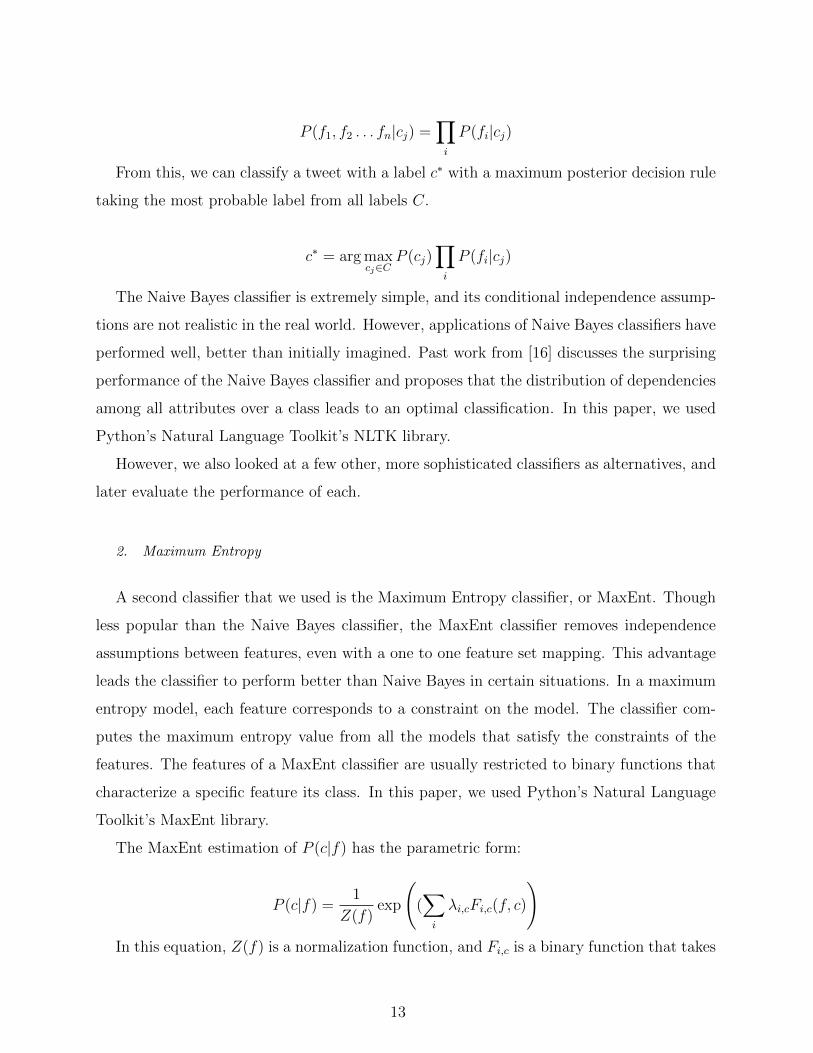
P (f1, f2 . . . fn|cj) =∏i

P (fi|cj)

From this, we can classify a tweet with a label c∗ with a maximum posterior decision rule

taking the most probable label from all labels C.

c∗ = arg maxcj∈C

P (cj)∏i

P (fi|cj)

The Naive Bayes classifier is extremely simple, and its conditional independence assump-

tions are not realistic in the real world. However, applications of Naive Bayes classifiers have

performed well, better than initially imagined. Past work from [16] discusses the surprising

performance of the Naive Bayes classifier and proposes that the distribution of dependencies

among all attributes over a class leads to an optimal classification. In this paper, we used

Python’s Natural Language Toolkit’s NLTK library.

However, we also looked at a few other, more sophisticated classifiers as alternatives, and

later evaluate the performance of each.

2. Maximum Entropy

A second classifier that we used is the Maximum Entropy classifier, or MaxEnt. Though

less popular than the Naive Bayes classifier, the MaxEnt classifier removes independence

assumptions between features, even with a one to one feature set mapping. This advantage

leads the classifier to perform better than Naive Bayes in certain situations. In a maximum

entropy model, each feature corresponds to a constraint on the model. The classifier com-

putes the maximum entropy value from all the models that satisfy the constraints of the

features. The features of a MaxEnt classifier are usually restricted to binary functions that

characterize a specific feature its class. In this paper, we used Python’s Natural Language

Toolkit’s MaxEnt library.

The MaxEnt estimation of P (c|f) has the parametric form:

P (c|f) =1

Z(f)exp

((∑i

λi,cFi,c(f, c)

)In this equation, Z(f) is a normalization function, and Fi,c is a binary function that takes

13

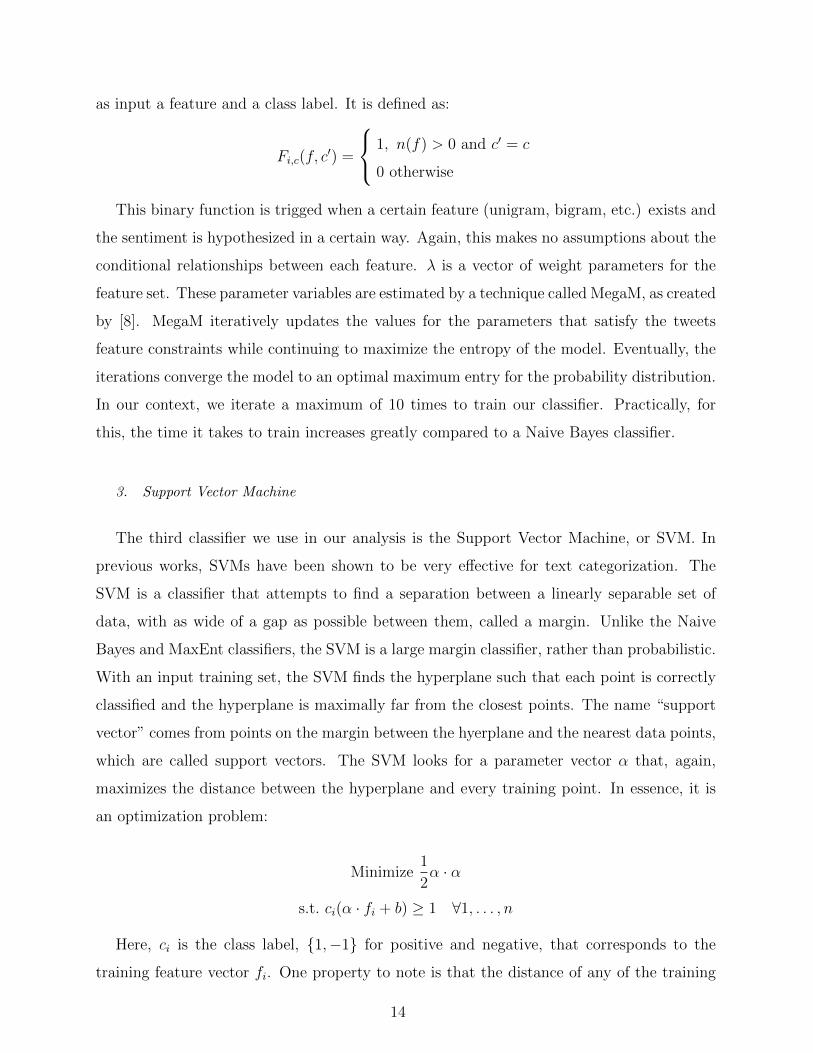
as input a feature and a class label. It is defined as:

Fi,c(f, c′) =

1, n(f) > 0 and c′ = c

0 otherwise

This binary function is trigged when a certain feature (unigram, bigram, etc.) exists and

the sentiment is hypothesized in a certain way. Again, this makes no assumptions about the

conditional relationships between each feature. λ is a vector of weight parameters for the

feature set. These parameter variables are estimated by a technique called MegaM, as created

by [8]. MegaM iteratively updates the values for the parameters that satisfy the tweets

feature constraints while continuing to maximize the entropy of the model. Eventually, the

iterations converge the model to an optimal maximum entry for the probability distribution.

In our context, we iterate a maximum of 10 times to train our classifier. Practically, for

this, the time it takes to train increases greatly compared to a Naive Bayes classifier.

3. Support Vector Machine

The third classifier we use in our analysis is the Support Vector Machine, or SVM. In

previous works, SVMs have been shown to be very effective for text categorization. The

SVM is a classifier that attempts to find a separation between a linearly separable set of

data, with as wide of a gap as possible between them, called a margin. Unlike the Naive

Bayes and MaxEnt classifiers, the SVM is a large margin classifier, rather than probabilistic.

With an input training set, the SVM finds the hyperplane such that each point is correctly

classified and the hyperplane is maximally far from the closest points. The name “support

vector” comes from points on the margin between the hyerplane and the nearest data points,

which are called support vectors. The SVM looks for a parameter vector α that, again,

maximizes the distance between the hyperplane and every training point. In essence, it is

an optimization problem:

Minimize1

2α · α

s.t. ci(α · fi + b) ≥ 1 ∀1, . . . , n

Here, ci is the class label, {1,−1} for positive and negative, that corresponds to the

training feature vector fi. One property to note is that the distance of any of the training

14

points from the hyperplane margin will be no less than 1||α|| . The solution of the problem

can be written as:

w =∑j

αjcjdj, αj ≥ 0

Once the SVM is built, classification of new tweets simply involves determining which

side of the hyperplane that they fall on. In our case, there are only two classes, so there is

no need to go to a non-linear classifier. However, the SVM is flexible in non-linear situations

using the kernel trick, which transforms their input into a higher dimensional space.

VII. CLASSIFIER EVALUATION

To continue to our ultimate goal of applying Twitter sentiment to the financial market,

we trained and tested each of our classifiers on a subset of our tweet corpus. Though we

gathered a few hundred thousand tweets, we were only able to train on a few thousand, due

to memory constraints. In the future, work on memory optimizations and more powerful or

distributed machines should allow us to train on more data.

For each of the classifiers, performed a 4-fold cross validation and found the average

accuracy. N-fold cross validation means splitting the training data into N sets. One of those

sets is left out as a test set to measure accuracy, and the N-1 other sets are used to train the

classifier. This is repeated N total times, one for each separate data partition. Afterwards,

the accuracies were averaged and reported.

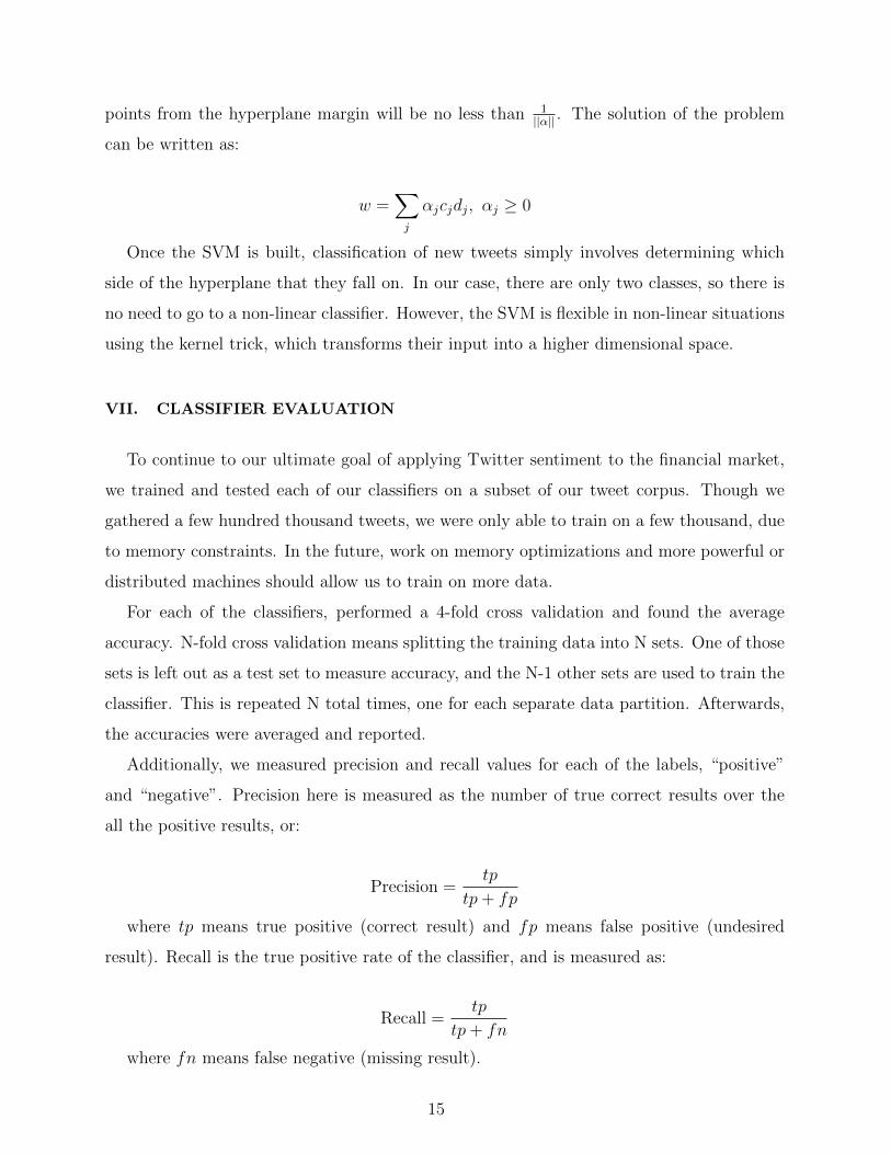
Additionally, we measured precision and recall values for each of the labels, “positive”

and “negative”. Precision here is measured as the number of true correct results over the

all the positive results, or:

Precision =tp

tp+ fp

where tp means true positive (correct result) and fp means false positive (undesired

result). Recall is the true positive rate of the classifier, and is measured as:

Recall =tp

tp+ fn

where fn means false negative (missing result).

15

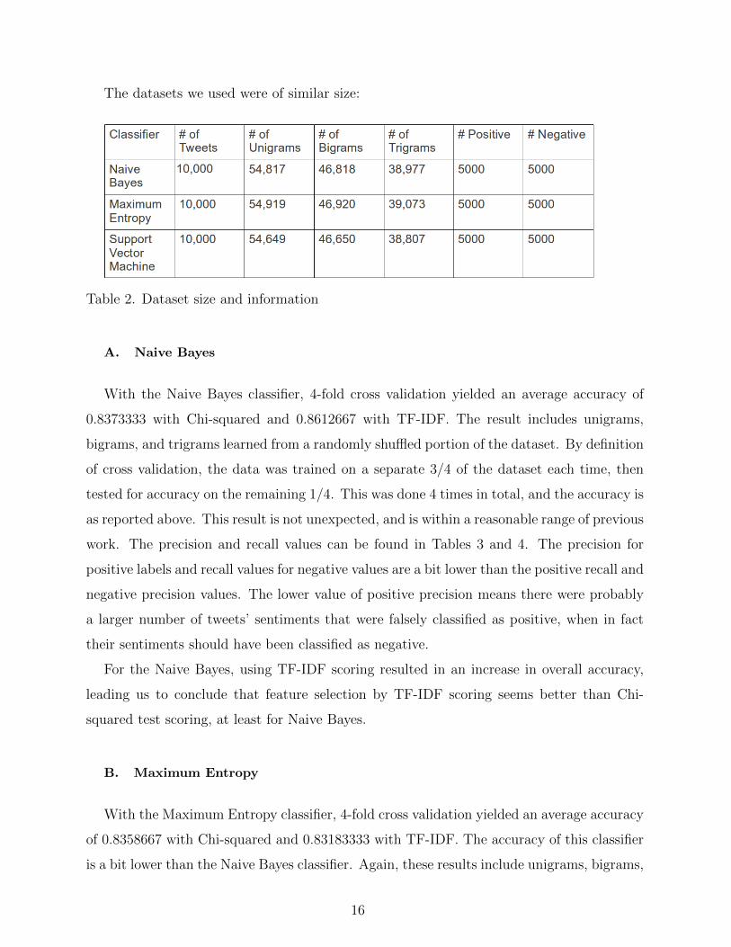
The datasets we used were of similar size:

Table 2. Dataset size and information

A. Naive Bayes

With the Naive Bayes classifier, 4-fold cross validation yielded an average accuracy of

0.8373333 with Chi-squared and 0.8612667 with TF-IDF. The result includes unigrams,

bigrams, and trigrams learned from a randomly shuffled portion of the dataset. By definition

of cross validation, the data was trained on a separate 3/4 of the dataset each time, then

tested for accuracy on the remaining 1/4. This was done 4 times in total, and the accuracy is

as reported above. This result is not unexpected, and is within a reasonable range of previous

work. The precision and recall values can be found in Tables 3 and 4. The precision for

positive labels and recall values for negative values are a bit lower than the positive recall and

negative precision values. The lower value of positive precision means there were probably

a larger number of tweets’ sentiments that were falsely classified as positive, when in fact

their sentiments should have been classified as negative.

For the Naive Bayes, using TF-IDF scoring resulted in an increase in overall accuracy,

leading us to conclude that feature selection by TF-IDF scoring seems better than Chi-

squared test scoring, at least for Naive Bayes.

B. Maximum Entropy

With the Maximum Entropy classifier, 4-fold cross validation yielded an average accuracy

of 0.8358667 with Chi-squared and 0.83183333 with TF-IDF. The accuracy of this classifier

is a bit lower than the Naive Bayes classifier. Again, these results include unigrams, bigrams,

16

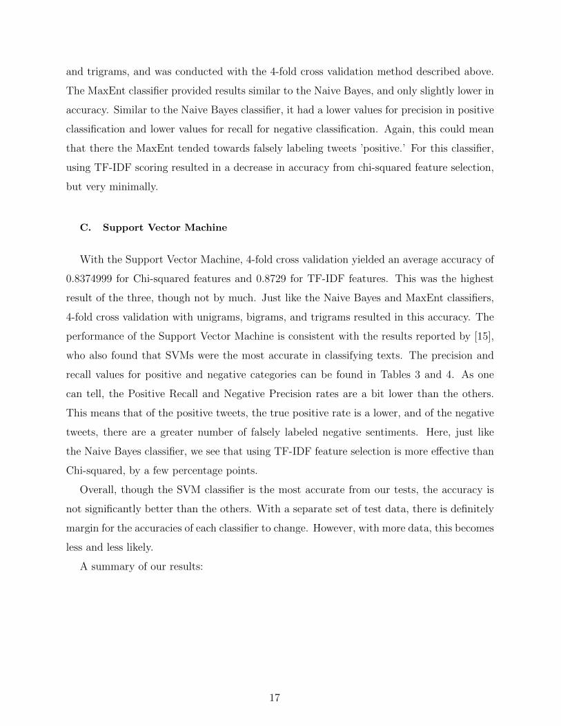
and trigrams, and was conducted with the 4-fold cross validation method described above.

The MaxEnt classifier provided results similar to the Naive Bayes, and only slightly lower in

accuracy. Similar to the Naive Bayes classifier, it had a lower values for precision in positive

classification and lower values for recall for negative classification. Again, this could mean

that there the MaxEnt tended towards falsely labeling tweets ’positive.’ For this classifier,

using TF-IDF scoring resulted in a decrease in accuracy from chi-squared feature selection,

but very minimally.

C. Support Vector Machine

With the Support Vector Machine, 4-fold cross validation yielded an average accuracy of

0.8374999 for Chi-squared features and 0.8729 for TF-IDF features. This was the highest

result of the three, though not by much. Just like the Naive Bayes and MaxEnt classifiers,

4-fold cross validation with unigrams, bigrams, and trigrams resulted in this accuracy. The

performance of the Support Vector Machine is consistent with the results reported by [15],

who also found that SVMs were the most accurate in classifying texts. The precision and

recall values for positive and negative categories can be found in Tables 3 and 4. As one

can tell, the Positive Recall and Negative Precision rates are a bit lower than the others.

This means that of the positive tweets, the true positive rate is a lower, and of the negative

tweets, there are a greater number of falsely labeled negative sentiments. Here, just like

the Naive Bayes classifier, we see that using TF-IDF feature selection is more effective than

Chi-squared, by a few percentage points.

Overall, though the SVM classifier is the most accurate from our tests, the accuracy is

not significantly better than the others. With a separate set of test data, there is definitely

margin for the accuracies of each classifier to change. However, with more data, this becomes

less and less likely.

A summary of our results:

17

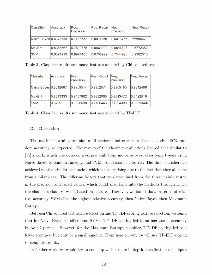
Table 3. Classifier results summary, features selected by Chi-squared test

Table 4. Classifier results summary, features selected by TF-IDF

D. Discussion

The machine learning techniques all achieved better results than a baseline 50% ran-

dom accuracy, as expected. The results of the classifier evaluations showed that similar to

[15]’s work, which was done on a corpus built from movie reviews, classifying tweets using

Naive Bayes, Maximum Entropy, and SVMs could also be effective. The three classifiers all

achieved relative similar accuracies, which is unsurprising due to the fact that they all come

from similar data. The differing factors that we determined from the three mainly rested

in the precision and recall values, which could shed light into the methods through which

the classifiers classify tweets based on features. However, we found that, in terms of rela-

tive accuracy, SVMs had the highest relative accuracy, then Naive Bayes, then Maximum

Entropy.

Between Chi-squared test feature selection and TF-IDF scoring feature selection, we found

that for Naive Bayes classifiers and SVMs, TF-IDF scoring led to an increase in accuracy

by over 2 percent. However, for the Maximum Entropy classifier, TF-IDF scoring led to a

lower accuracy, but only by a small amount. From here on out, we will use TF-IDF scoring

to compute results.

In further work, we would try to come up with a more in depth classification techniques

18

for determining a ’neutral’ label. One of the reasons that we decided against a neutral tweet

label was due to the difficulty of determining a method to train the neutral label, as we did

not know where or how to find neutral tweets. In other words, we encountered difficulty in

automatically finding and building a training set of data. Simply forming a bag of words

with ’objective’ words would not be sufficient, as this would probably add noise to proper

’positive’ and ’negative’ tweet classifications. Instead there would need to be more work

done in determining a more effective way of determining neutrality.

Additionally, one weakness of our system is that it does not take into account negations

very well. For example, if a tweet has the word ’like’ in it, it could be labeled as positive,

even if the whole phrase said ’don’t like.’ A human being could differentiate this within a

second, but our classifiers cannot. An improvement on this would to go deeper into looking

for such phrases and adding their presence as a feature.

Overall, the Naive Bayes classifier, Maximum Entropy classifier, and Support Vector

Machine all proved effective classifiers of tweets into ’positive’ and ’negative’ sentiments.

We did realize a few flaws with our classification after the fact, but we were still able to

show that each classification technique was able to be applied to tweet n-grams with a high

level of accuracy.

VIII. MARKET CORRELATION

After training and saving our classifier, we decided that an interesting application would

be to look at correlation between tweet sentiment and stock market prices on an intra-day

scale. To do so, we first had to build a system to collect stock data, as well as tweets during

market hours. For the scope of the project, we decided to look for intra-day correlation with

a lag period of k minutes. Additionally, we focused our scope only on technology stocks.

Therefore, we gathered minute by minute data on a few of the most popular technology

ETFs.

A. Stock Mining

ETFs, or exchange traded funds, generally track an index. This way, they are good

representations of the state of an entire market. We used Yahoo’s finance API to gather

19

data on 10 ETFs throughout the trading day, which was 8:30-3:00 PM Central time. Yahoo’s

data was lagged by 15 minutes, so we had to accommodate for that while computing our

correlation lag values. We store each gathered price and its timestamp in a MongoDB

collection, for later processing.

B. Tweet Mining

In a similar manner to gathering our tweet corpus from above, we used Twitter’s search

API to gather tweets about technology from 8:30-3:00 PM Central time, same as market

hours. The keywords we used were: technology and stocks. These keywords were chosen

arbitrarily, and in future work, would best be integrated with the post-correlated keywords

part of the project. However, they accurately reflected a variety of topics and generally

provided an on-topic set of tweets to analyze.

Again, we stored the gathered tweets in a MongoDB collection. After gathering the

tweets, we classified each of them using our saved classifier and stored the results in another

database collection.

C. Methods

After collecting our data from the sources mentioned above, we worked to look for corre-

lation between sentiment and stock prices. To do this, we follow a procedure:

1. Associate each tweet and each stock price with a timestamp, measured to the closest

minute.

2. For each twitter minute, compute a sentiment score.

3. Normalize both the twitter sentiment scores and the stock prices.

4. Choose a set of lag values, k, to iterate through. (With the +15 minute Yahoo lag

compensation)

5. For each lag value specified, compute the correlation between the twitter sentiment

score and stock market price.

6. Keep track of the strongest correlated lags, and return

20

Each correlation compares two time series, stock price and tweet sentiment, and is offset

by a certain lag value. This means that we delayed prices by a certain time, for each

correlation calculation to account for any time difference required for twitter sentiment to

be reflected in stock prices. The equation for correlation we used was:

rxy =

n∑i=0

(xi − x)(yi − y)√n∑i=0

(xi − x)2(yi − y)2

This is also called the Pearson correlation coefficient.

To calculate the sentiment score, we simply took the ratio between positive and total

sentiments. If there were no negative sentiments, the ratio would be 1. Conversely, if there

was less positive sentiment, the ratio would be closer to 0.

D. Correlation Results

We used lag values between 0 and 90, incremented by 10. For each of them, we calcu-

lated the Pearson correlation. The results of intra-day correlation were disappointing, but

unsurprising. We ultimately found that there was almost no correlation between intraday

tweets of any lag value.

21

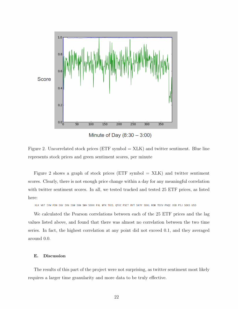
Figure 2. Uncorrelated stock prices (ETF symbol = XLK) and twitter sentiment. Blue line

represents stock prices and green sentiment scores, per minute

Figure 2 shows a graph of stock prices (ETF symbol = XLK) and twitter sentiment

scores. Clearly, there is not enough price change within a day for any meaningful correlation

with twitter sentiment scores. In all, we tested tracked and tested 25 ETF prices, as listed

here:

We calculated the Pearson correlations between each of the 25 ETF prices and the lag

values listed above, and found that there was almost no correlation between the two time

series. In fact, the highest correlation at any point did not exceed 0.1, and they averaged

around 0.0.

E. Discussion

The results of this part of the project were not surprising, as twitter sentiment most likely

requires a larger time granularity and more data to be truly effective.

22

Our time granularity was much too small for public opinion to be reflected in market

changes. For all of the ETFs we looked at, there was very little change throughout the

course of the day. On the other hand, the Twitter sentiment scores varied greatly, probably

due to the small sample size due to the separation of minute by minute data. As you can

see in Figure 2, the blue line represents stock prices and the green the sentiment score, by

minute. Clearly, the time scale is too small for any meaningful correlation. In previous

works, correlations were observed, but they were over a much longer period of time. For

example, in [4], where the most meaningful correlation was reported, the data was gathered

for 10 months, then analyzed on a day to day scale, rather than minute by minute.

In future work, using our same approach, we will be able to use our system over a longer

period of time to find deeper correlations. For example, tweets gathered over a year could

be analyzed on a week to week sentiment level to find more meaningful correlation. Twitter

sentiment works best on a larger scale, with more aggregate data. Because of this, with a

longer time period, there would be more tweets as well, leading to a more balanced and less

volatile sentiment level for tweets.

IX. SIGNIFICANT KEYWORD CORRELATION

After gathering a significant amount of tweets and price information, we decided to

additionally look for correlation between significant words and stock prices. Because of

our difficulty coming up with the best related keywords for twitter, we realized there was a

parallel problem we could solve with our data. This time, instead of looking for a correlation

between stock prices and tweet sentiments, we decided to work backwards and examine which

specific words from tweets were associated with changes in stock prices.

A. Methods

We need no additional data to perform this task. We have already gathered our technol-

ogy related tweets, and have our stock prices. Again, we are looking to see which specific

words seem to lead to a change in stock prices. To do this, we:

1. Associate each tweet and each stock price with a timestamp, measured to the closest

minute.

23

2. Choose a set of lag values, k, to iterate through. (With the +15 minute Yahoo lag

compensation)

3. Initialize a dictionary mapping individual words to a score (initially 0) for every minute

m.

4. For each minute m, compute the difference in current stock price, d, with the price

after a certain lag.

5. Every word per tweet at minute m adds d to their score.

6. Afterwards, return the words with highest and lowest total scores.

We are only interested in the extremes, as the highest score indicates words which are

associated with positive stock price change, while the lowest scores are associated with

negative stock price change. At the end of iterating through each minute in a market day

for a number of lag values, we are left with a list of words which are most strongly correlated

with stock price change, either positive or negative.

B. Significant Keyword Results

We discovered meaningful and interesting results with the post-facto keyword correlation.

Our data consisted of two weeks worth of tweets gathered in the same manner as above.

We used lag values from 0-90, incremented by 10, and looked for the strongest keyword

scores for each of them. Bigrams and Trigrams were included in this correlation. For

each day and each lag value, we ranked the top twenty n-grams that led to positive stock

price change and top twenty n-grams that led to negative price change. As you can see,

there is overlap between some of the n-grams, as some unigrams are subsets of bigrams, or

bigrams of trigrams, etc. There are too many days of results to discuss, so Tables 5 and 6

show a representative sample of our results, sorted by most impactful to least impactful for

negative deltas, and vice versa for positive deltas.

24

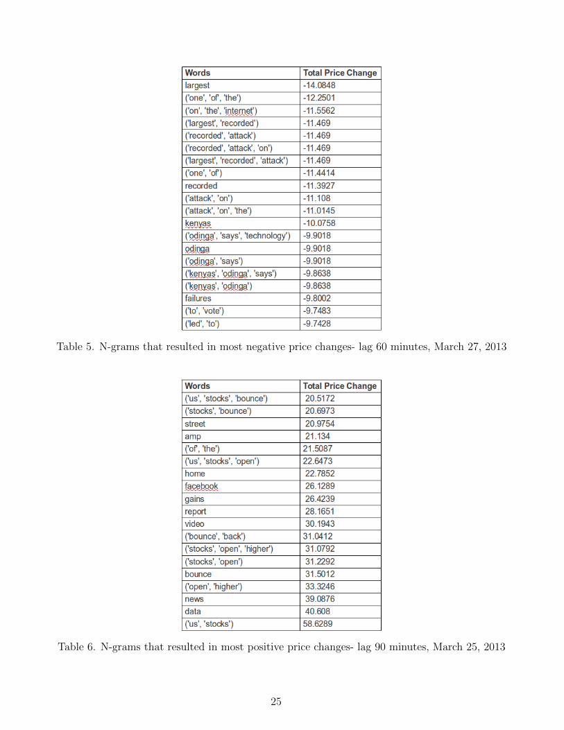
Table 5. N-grams that resulted in most negative price changes- lag 60 minutes, March 27, 2013

Table 6. N-grams that resulted in most positive price changes- lag 90 minutes, March 25, 2013

25

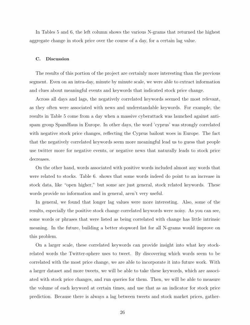
In Tables 5 and 6, the left column shows the various N-grams that returned the highest

aggregate change in stock price over the course of a day, for a certain lag value.

C. Discussion

The results of this portion of the project are certainly more interesting than the previous

segment. Even on an intra-day, minute by minute scale, we were able to extract information

and clues about meaningful events and keywords that indicated stock price change.

Across all days and lags, the negatively correlated keywords seemed the most relevant,

as they often were associated with news and understandable keywords. For example, the

results in Table 5 come from a day when a massive cyberattack was launched against anti-

spam group SpamHaus in Europe. In other days, the word ’cyprus’ was strongly correlated

with negative stock price changes, reflecting the Cyprus bailout woes in Europe. The fact

that the negatively correlated keywords seem more meaningful lead us to guess that people

use twitter more for negative events, or negative news that naturally leads to stock price

decreases.

On the other hand, words associated with positive words included almost any words that

were related to stocks. Table 6. shows that some words indeed do point to an increase in

stock data, like “open higher,” but some are just general, stock related keywords. These

words provide no information and in general, aren’t very useful.

In general, we found that longer lag values were more interesting. Also, some of the

results, especially the positive stock change correlated keywords were noisy. As you can see,

some words or phrases that were listed as being correlated with change has little intrinsic

meaning. In the future, building a better stopword list for all N-grams would improve on

this problem.

On a larger scale, these correlated keywords can provide insight into what key stock-

related words the Twitter-sphere uses to tweet. By discovering which words seem to be

correlated with the most price change, we are able to incorporate it into future work. With

a larger dataset and more tweets, we will be able to take these keywords, which are associ-

ated with stock price changes, and run queries for them. Then, we will be able to measure

the volume of each keyword at certain times, and use that as an indicator for stock price

prediction. Because there is always a lag between tweets and stock market prices, gather-

26

ing tweets and determining the volumes of keywords that are most interesting could have

implications for later stock market prices.

X. OVERALL CHALLENGES

Throughout the course of the project, we ran across a number of challenges. The scope

of the challenges varied greatly, and we were able to overcome some, but not all.

The first challenge we discovered was a matter of tweet searching. Though we had a

system set up to process tweets, it was difficult to choose the right keywords to search on.

In the end, our method was a bit arbitrary, for we had no stronger alternative. We tried

using different stock symbols to collect our tweets, but Though the keywords chosen matter

less and less with a larger amount of tweets, they still play a large role in determining how

much correlation there is between tweet sentiment and stock market prices.

Another inherent challenge with twitter sentiment is differentiating between slang or

jargon and real English. For example, many people substitute “your” with “ur,” or “hello”

with “yo.” Though we are able to understand slang when we read it, it is harder for a

computer to understand. Therefore, many important, sentiment-contributing words are

potentially lost. This is a challenging problem to solve, and perhaps more work will be done

on it in the future.

Additionally, we ran into the challenge of computation time and power. Because we

didn’t have immediate access to large amounts of storage, we trained many of our classifiers

on a limited number of tweets. Though the system is able to train on much more data, we

didn’t have the time or computation power at hand. This challenge can be addressed by

taking the project to a larger scale, over a few years. This way, there would be more data

to train on and more time to do the training.

XI. FUTURE WORK

There are many areas in which this work could be expanded on in the future. With a

longer period of time and more resources, there is much potential in the area.

One idea for future improvement is to gather data for a longer period of time, and with

different granularities. One of the shortcomings of this study was the lack of time needed

27

(years) for best data collection. If possible, we would want to collect data over the course

of a few years, both from Twitter and the stock market. This way, we could also alter

the granularity of the data. Instead of looking at intraday trends between Twitter and

the stock market, we would be able to look at larger scales of correlation, between days or

weeks. Intuitively, we feel that decreasing the granularity of the data would provide for a

stronger correlation, as the sentiment would be more accurate. Also, sentiment, a macro

measurement, may take a while to manifest itself in the stock market- more than just in a

few minutes or hours. We would be able to have more tweets for both training and analyzing,

also, from a longer period of time.

Another natural expansion of the project would be to actually make stock predictions

and trade money based on twitter sentiment. To do this, w would follow some existing

examples of using a Neural Network for prediction. However, we would not want to solely

rely on twitter sentiment- we would want to incorporate other technical indicators. This is

quite a bit more research and knowledge, and was out of scope of this project. Nevertheless,

it would be an interesting area of future study, as the options and opportunities in the area

of stock price prediction are endless.

Lastly, another area of future work would be to better incorporate the significant words

determined by this paper into the keywords used to look for technology related tweets.

Naturally, by first discovering which individual words seem to correlate to changes in stock

prices, and then building a dataset from those words, we might be able to see a stronger

correlation to certain stocks. Though this is more narrow of a project and would be less

generalizable, it would be more practical for real money trading. The words may only relate

to a specific stock or set of stocks, but that would be okay.

Acknowledgments

This project would not have been possible without the guidance of Dr. Inderjit Dhillon,

the advisor for this study. Additionally, thanks go out to Dr. Aziz Adnan for his mentorship,

and Dr. William Press for assisting on the Undergraduate Thesis Comittee. Lastly, thanks

to my team in 1 Semester Startup- Ashton Grimball, George Su, and Patrick Day, for

28

introducing me to this area of research.

[1] Sentiwordnet, an enhanced lexical resource for sentiment analysis and opinion mining.

[2] Stefano Baccianella, Andrea Esuli, and Fabrizio Sebastiani. Sentiwordnet 3.0: An enhanced

lexical resource for sentiment analysis and opinion mining. 2010.

[3] Albert Bifet and Eibe Frank. Sentiment knowledge discovery in twitter streaming data. 2011.

[4] J. Bollen and H. Mao. Twitter mood as a stock market predictor. IEEE Computer, 44(10):91–

94, 2010.

[5] A. Bromberg. Sentiment analysis in python. 2013.

[6] Eric D. Brown. Will twitter make you a better investor? a look at sentiment, user reputation

and their effect on the stock market. SAIS Proceedings, 2012.

[7] Ray Chen and Marius Lazer. Sentiment analysis of twitter feeds for the prediction of stock

market movement. 2012.

[8] Hal Daum. Notes on cg and lm-bfgs optimization of logistic regression. 2004.

[9] Shangkun Deng, Takashi Mitsubuchi, Kei Shioda, Tatsuro Shimada, and Akito Sakurai. Com-

bining technical analysis with sentiment analysis for stock price prediction. In Proceedings of

the 2011 IEEE Ninth International Conference on Dependable, Autonomic and Secure Com-

puting, pages 800–807, EEE Computer Society, Washington, DC, USA., 2011. DASC ’11 IEEE

Computer Society.

[10] S. Elson, D. Yeung, R. Parisa, S. . R. Bohandy, and A. Nader. Using social media to gauge

iranian public opinion and mood after the 2009 election. 2012.

[11] Ronen Feldman. Techniques and applications for sentiment analysis. Communications of the

ACM, 56(4):82–89, 2013.

[12] E. Hurwitz and T. Marwala. Common mistakes when applying computational intelligence and

machine learning to stock market modelling. 2012.

[13] Anshul Mittal and Arpit Goel. Stock prediction using twitter sentiment analysis. 2012.

[14] Alexander Pak and Patrick Paroubek. Twitter as a corpus for sentiment analysis and opinion

mining. Proceedings of LREC, 2010.

[15] B. Pang, L. Lee, and S. Vaithyanathan. Thumbs up? sentiment classification using machine

learning techniques. pages 79–86, 2002.

29

[16] DongSong Zhang and Lina Zhou. Discovering golden nuggets: Data mining in financial appli-

cation. Systems, Man, and Cybernetics, Part C: Applications and Reviews, IEEE Transactions

on, 34(4):513–22, 2004.

30