Sensors to Monitor Bond in Concrete Bridges Rehabilitated with FRP

Final Report to the Michigan Department of Transportation

by

Ronald S. Harichandran Professor and Chairperson

and

Sangdo Hong

Graduate Student

October 2003

Department of Civil and Environmental Engineering Michigan State University

East Lansing, MI 48824-1226

Tel: (517) 355-5107 Fax: (517) 432-1827

E-Mail: harichan@egr.msu.edu Web: www.egr.msu.edu/cee/~harichan

1. Report No.

Research Report RC- 1435 2. Government Accession No.

3. MDOT Project Manager: Roger Till

4. Title and Subtitle: Sensors to Monitor Bond in Concrete Bridges Rehabilitated with FRP

5. Report Date: 8/31/03

7. Author(s): Ronald Harichandran & Sangdo Hong

6. Performing Organization Code

9. Performing Organization Name and Address

Department of Civil and Environmental Engineering Michigan State University East Lansing, MI 4824-1226

8. Performing Org Report No.

10. Work Unit No. (TRAIS)

11. Contract Number: 01-0365

12. Sponsoring Agency Name and Address

Michigan Department of Transportation Construction and Technology Division P.O. Box 30049 Lansing, MI 48909

11(a). Authorization Number:

13. Type of Report & Period Covered Research Report, 2/15/01 to 8/31/03

15. Supplementary Notes

14. Sponsoring Agency Code

16. Abstract: Electrochemical impedance spectroscopy (EIS) based sensor technology is used for the NDE of the bond between external CFRP reinforcement and concrete in beams. Copper tape on the surface of the CFRP sheet, stainless steel wire embedded in the concrete, and reinforcing bars were used as the sensing elements. Laboratory experiments were designed to test the capability of the sensors to detect the debonding of the CFRP from the concrete and to study the effect of short-term (humidity and temperature fluctuations and chloride content) and long-term (freeze-thaw and wet-dry exposure and rebar corrosion) environmental conditions on the measurements. The CFRP sheet was debonded from the concrete and impedance measurements were taken between various pairs of electrodes at various interfacial crack lengths. The dependence of the impedance spectra, and of the parameters obtained from equivalent circuit analysis, on the interfacial crack length was studied. Capacitance parameters in the equivalent circuit were used to assess the global state of the bond between CFRP sheets and concrete. Impedance measure-ments taken between embedded wire sensors were used to detect the location of debonded regions. Although the measurements are sensitive to short- and long-term environmental effects, measurements at high frequencies and the capacitance parameters resulting from equivalent circuit analysis are insensitive to these factors.

17. Key Words: NDE, EIS, CFRP sheet, sensors, debonding,

18. Distribution Statement No restrictions. This document is available to the public through the Michigan Department of Transportation.

19. Security Classification (report) Unclassified

20. Security Classification (Page) Unclassified

21. No of Pages 22. Price

ABSTRACT

Electrochemical impedance spectroscopy (EIS) based sensor technology is used for

the NDE of the bond between external CFRP reinforcement and concrete in beams.

Copper tape on the surface of the CFRP sheet, stainless steel wire embedded in the

concrete, and reinforcing bars were used as the sensing elements. Laboratory experiments

were designed to test the capability of the sensors to detect the debonding of the CFRP

from the concrete and to study the effect of short-term (humidity and temperature

fluctuations and chloride content) and long-term (freeze-thaw and wet-dry exposure and

rebar corrosion) environmental conditions on the measurements. The CFRP sheet was

debonded from the concrete and impedance measurements were taken between various

pairs of electrodes at various interfacial crack lengths. The dependence of the impedance

spectra, and of the parameters obtained from equivalent circuit analysis, on the interfacial

crack length was studied. Capacitance parameters in the equivalent circuit were used to

assess the global state of the bond between CFRP sheets and concrete. Impedance

measurements taken between embedded wire sensors were used to detect the location of

debonded regions.

i

ACKNOWLEDGMENTS

This research was funded by Michigan State Department of Transportation. This

contribution is gratefully acknowledged. The project manager was Roger Till. His

feedback throughout the project is appreciated.

ii

TABLE OF CONTENTS

LIST OF TABLES...................................................................................................... vi

LIST OF FIGURES .................................................................................................. vii

Chapter 1 Introduction..................................................................................................... 1 1.1 BACKGROUND........................................................................................................... 2 1.2 ELECTROCHEMICAL IMPEDANCE SPECTROSCOPY – BACKGROUND........................... 4

1.2.1 Impedance ........................................................................................................ 4 1.2.2 Electrochemical impedance spectroscopy and equivalent circuit

analysis............................................................................................................... 6 1.3 USE OF EIS FOR DETECTION OF INTERFACIAL DEGRADATION—A

LITERATURE REVIEW ................................................................................................. 8 1.4 HYPOTHESIS AND OBJECTIVES ................................................................................ 16

Chapter 2 Experimental Design .................................................................................... 17 2.1 SPECIMEN PREPARATION AND SENSOR CONFIGURATION ........................................ 18

2.1.1 Specimen sizes and preparation ..................................................................... 18 2.1.2 Sensor configuration and installation............................................................. 21 2.1.3 Sensor combinations for impedance measurements....................................... 23

2.2 DETECTION OF FRP DEBONDING ............................................................................ 24 2.2.1 Two foot long specimens ............................................................................... 24 2.2.2 Large beam specimen..................................................................................... 25

2.3 ASSESSMENT OF THE SENSITIVITY OF SENSOR MEASUREMENTS TO ENVIRONMENTAL EFFECTS ...................................................................................... 26 2.3.1 Humidity......................................................................................................... 26 2.3.2 Temperature ................................................................................................... 26 2.3.3 Chloride content ............................................................................................. 27 2.3.4 Freeze – thaw ................................................................................................. 29 2.3.5 Wetting and drying......................................................................................... 29 2.3.6 Corrosion of reinforcing bar........................................................................... 30

2.4 ELECTRODE SIZE EFFECTS ....................................................................................... 33

Chapter 3 Experimental Results, Equivalent Circuit Analysis, and Discussion....... 35 3.1 EQUIVALENT CIRCUIT.............................................................................................. 35 3.2 CFRP DEBONDING ................................................................................................. 40

3.2.1 Results for 2-foot long specimens .................................................................. 40 3.2.1.1 Comparison of raw impedance spectra................................................... 44 3.2.1.2 Results from equivalent circuit analysis................................................. 44

3.2.2 Results for 8-foot long specimen ................................................................... 49 3.2.2.1 Comparison of raw impedance spectra................................................... 49 3.2.2.2 Results from equivalent circuit analysis................................................. 50

3.2.3 Detecting the location of debonded regions................................................... 55 3.2.3.1 Comparison of raw impedance spectra................................................... 55 3.2.3.2 Results from equivalent circuit analysis................................................. 59

iii

3.2.4 Empirical Relationships ................................................................................. 61 3.2.4.1 Raw impedance spectra .......................................................................... 61 3.2.4.2 Equivalent circuit analysis...................................................................... 64

3.2.5 Summary and Discussion ............................................................................... 66 3.3 SENSITIVITY OF SENSOR MEASUREMENTS TO ENVIRONMENTAL EFFECTS .............. 68

3.3.1 Humidity......................................................................................................... 68 3.3.1.1 Comparison of raw impedance spectra................................................... 68 3.3.1.2 Results from equivalent circuit analysis................................................. 69 3.3.1.3 Summary and Discussion ....................................................................... 69

3.3.2 Temperature ................................................................................................... 74 3.3.2.1 Comparison of raw impedance spectra................................................... 74 3.3.2.2 Results from equivalent circuit analysis................................................. 78 3.3.2.3 Summary and Discussion ....................................................................... 78

3.3.3 Chloride content ............................................................................................. 81 3.1.3.1 Comparison of raw impedance spectra................................................... 81 3.3.3.2 Results from equivalent circuit analysis................................................. 87 3.3.3.3 Summary and Discussion ....................................................................... 87

3.3.4 Freeze – thaw ................................................................................................. 88 3.3.4.1 Comparison of raw impedance spectra................................................... 88 3.3.4.2 Results from equivalent circuit analysis................................................. 88 3.3.4.3 Summary and Discussion ....................................................................... 88

3.3.5 Wetting and drying......................................................................................... 92 3.3.5.1 Comparison of raw impedance spectra................................................... 92 3.3.5.2 Results from equivalent circuit analysis................................................. 92 3.3.5.3 Summary and Discussion ....................................................................... 92

3.3.6 Corrosion of reinforcing bar........................................................................... 96 3.3.6.1 Comparison of raw impedance spectra................................................... 96 3.3.6.2 Results from equivalent circuit analysis................................................. 97 3.3.6.3 Summary and Discussion ....................................................................... 97

3.4 EFFECT OF ELECTRODE SIZE .................................................................................. 101

Chapter 4 Summary, Conclusions, and recommendations for Future Work......... 103 4.1 SUMMARY............................................................................................................. 103

4.1.1 Detection of CFRP Debonding .................................................................... 104 4.1.2 Environmental effects .................................................................................. 106

4.2 CONCLUSIONS ....................................................................................................... 107 4.3 RECOMMENDATIONS FOR FUTURE WORK ............................................................. 109

REFERENCES ......................................................................................................... 111

Appendix—A................................................................................................................. 113

Data Collection and Equivalent Circuit Analysis Procedure ................................... 113 A-1 SOFTWARE PROCEDURE FOR DATA COLLECTION................................................. 113 A-2 EQUIVALENT CIRCUIT ANALYSIS PROCEDURE ...................................................... 114

Appendix—B ................................................................................................................. 117

iv

Field Installation of EIS Based Sensor on Concrete Beams .......................... 117 B – 1 MATERIALS: ...................................................................................................... 117 B-2 CONSTRUCTION METHODS: ........................................................................ 119

Appendix—C ................................................................................................................. 123

EIS Measurements and Interpretation ....................................................................... 123 C-1: GENERAL PROTOCOL........................................................................................... 123 C-2: PROTOCOL FOR INITIAL IMPEDANCE MEASUREMENTS ......................................... 123 C-3: PROTOCOL FOR IMPEDANCE MEASUREMENTS TO DETECT DEBONDING ................ 124

v

LIST OF TABLES

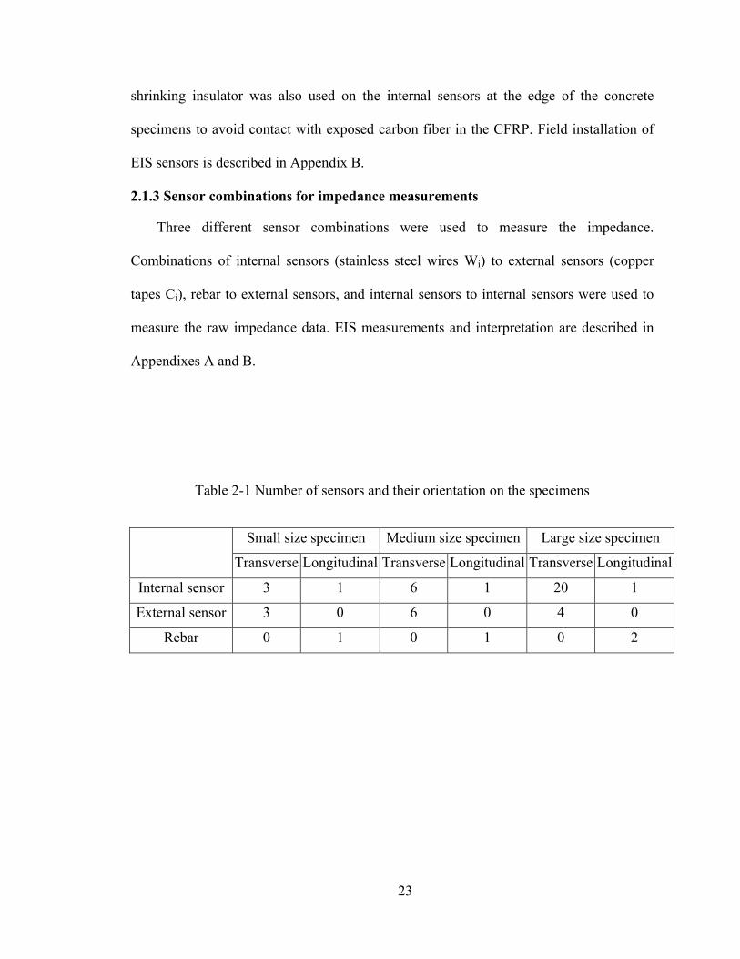
Table 2-1 Number of sensors and their orientation on the specimens.............................. 23

Table 3-1 Parameters of the curve fitted to measured impedance in the high-frequency range............................................................................................................ 62

Table 3-2 Parameters of the curve fitted to (C1+C2+C3) from equivalent circuit analysis......................................................................................................................... 64

Table 3-3 Specimen weights before and after freeze-thaw testing ................................... 89

Table 3-4 Specimen weights before and after wet-dry testing ......................................... 93

Table 3-5 Specimen weights before and after corrosion testing....................................... 98

vi

LIST OF FIGURES Figure 1-1 Typical electrochemical cell ........................................................................... 10

Figure 1-2 Model of the charge transfer process when the rebar and CFRP sheet (via external sensor) are used as electrodes......................................................................... 10

Figure 1-3 Equivalent circuit configurations — (a) simple circuit used for a corrosion reaction (Macdonald 1987) (b) circuit used to study an adhesive bond (Davis et al. 1999) ............................................................................................................................ 11

Figure 1-4 Typical impedance spectra taken from the wedge test (Source: Davis et al. 1999) ............................................................................................................................ 14

Figure 1-5 Resistance parameters from the equivalent circuit analysis as a function of time for the wedge tests under wet condition (Source: Davis et al. 1999)................... 14

Figure 1-6 Variation of capacitance parameter from the equivalent circuit analysis as a function of bonded area for wedge tests under —(a) dry condition (b) wet condition (Source: Davis et al. 1999)........................................................................... 15

Figure 2-1 Small concrete beam configuration and sensor locations ............................... 19

Figure 2-2 Medium concrete beam configuration and sensor locations ........................... 19

Figure 2-3 Large concrete beam configuration and sensor locations ............................... 20

Figure 2-4 Cross-section of large beam............................................................................ 21

Figure 2-5 Experimental design flow chart for humidity, temperature and chloride content effects .............................................................................................................. 28

Figure 2-6 Experimental setup for accelerated corrosion ................................................. 32

Figure 2-7 Concrete slab configuration and sensor locations........................................... 33

Figure 3-1 Equivalent circuit used to study CFRP debonding ......................................... 38

Figure 3-2 Fitted Bode magnitude and phase angle plots using the two equivalent circuits. Dots are the actual measured impedance from the rebar to an external sensor. Solid lines are the theoretical impedance using the equivalent circuit in Figure 3-1. The dotted lines are the theoretical impedance using the equivalent circuit in Figure 1-2 (b). ............................................................................................... 38

Figure 3-3 Fitting with the equivalent circuits. Dots are the actual measured impedances between two internal sensors. Solid lines are the theoretical impedances using the equivalent circuit in Figure 3-1. The dotted lines are the

vii

theoretical impedances using the equivalent circuit in Figure 1-2 (b). — (a) Bode magnitude and phase angle plot; (b) Nyquist plot. ...................................................... 39

Figure 3-4 Bode magnitude plot of typical impedance spectra measured from the rebar to copper tape for wedge test in controlled environment (legend gives the crack length in inches) ................................................................................................. 41

Figure 3-5 Bode magnitude plot of typical impedance spectra measured from the rebar to copper tape for wedge test in ambient environment (legend gives the crack length in inches) ................................................................................................. 41

Figure 3-6 Nyquist plot of typical impedance spectra measured from the rebar to copper tape for wedge test in controlled environment (legend gives the crack length in inches) ........................................................................................................... 42

Figure 3-7 Enlargement of Figure 3-6, showing variation of measure impedance in the low to mid- frequency range (legend gives the crack length in inches)................. 42

Figure 3-8 Nyquist plot of impedance spectra measured from the rebar to copper tape for wedge test in ambient environment (legend gives the crack length in inches) ...... 43

Figure 3-9 Variation of typical measured impedance from the rebar to copper tape for wedge test at 10,000 Hz.......................................................................................... 45

Figure 3-10 Variation of typical measured impedance from the rebar to copper tape for wedge test at 100 Hz............................................................................................... 45

Figure 3-11 Variation of typical measured impedance from the rebar to copper tape for wedge test at 1 Hz................................................................................................... 46

Figure 3-12 Variation of the CPE parameter for wedge test in the controlled environment for measurements from the rebar to external sensors ............................. 46

Figure 3-13 Variation of the CPE parameter for wedge test in ambient condition for measurements from the rebar to external sensors (Note: the CPE parameter for spec. 2 is measured in controlled environment)........................................................... 47

Figure 3-14 Variation of the C1 parameter from equivalent circuit analysis for wedge test from the rebar to external sensors ......................................................................... 47

Figure 3-15 Variation of the C2+C3 parameter from equivalent circuit analysis for wedge test from the rebar to external sensors .............................................................. 48

Figure 3-16 Variation of the C1+C2+C3 parameter from equivalent circuit analysis for wedge test from the rebar to external sensors ........................................................ 48

viii

Figure 3-17 Bode magnitude plot of typical impedance spectra measured from the rebar to copper tape for wedge test of the large beam (legend gives the crack length in inches) ........................................................................................................... 51

Figure 3-18 Enlargement of Figure 3-17, showing variation of measure impedance in the low-frequency range (legend gives the crack length in inches) ............................. 51

Figure 3-19 Nyquist plot of impedance spectra measured from the rebar to copper tape for wedge test of large beam in ambient environment (legend gives the crack length in inches) ........................................................................................................... 52

Figure 3-20 Enlargement of Figure 3-17 showing variation of measured impedance in the high-frequency range (legend gives the crack length in inches)........................ 52

Figure 3-21 Bode magnitude plot of typical impedance spectra measured from the rebar to copper tape and the stainless steel bar to copper tape for wedge test of the large beam (legend gives the crack length in inches) .................................................. 53

Figure 3-22 Variation of typical measured impedance from the rebar to copper tape for wedge test at 100,000 Hz........................................................................................ 53

Figure 3-23 Variation of the CPE parameter from equivalent circuit analysis for the large specimen from the rebar to external sensor......................................................... 54

Figure 3-24 Variation of the capacitance parameters from equivalent circuit analysis for the large specimen from the rebar to external sensor ............................................. 54

Figure 3-25 Bode magnitude plot of impedance spectra measured between pairs of internal sensors for eight-foot specimen in ambient condition when crack tip was between sensors W2 and W3 (legend shows the internal sensors used)...................... 57

Figure 3-26 Bode magnitude plot of impedance spectra measured between pairs of internal sensors for two-foot specimen in ambient condition when crack tip was between sensors W3 and W4 (legend shows the internal sensors used)...................... 57

Figure 3-27 Nyquist plot of impedance spectra measured between pairs of internal sensors for two-foot specimen in ambient condition when crack tip was between sensors W3 and W4 (legend shows the internal sensors used) .................................... 58

Figure 3-28 Bode magnitude plot of impedance spectra measured between pairs of internal sensors for eight-foot specimen in ambient condition when crack tip was between sensors W5 and W6 (legend shows the internal sensors used)...................... 58

Figure 3-29 Variation of the CPE parameter for pairs of internal sensors for the 8-foot beam when crack tip was between sensors W2 and W3 (name of the bar shows the internal sensors used) .................................................................................. 60

ix

Figure 3-30 Variation of the CPE parameter for pairs of internal sensors for the 2-foot long beam when crack tip was between sensors W3 and W4 (name of the bar shows the internal sensors used) .................................................................................. 60

Figure 3-31 Fit of the measured impedance for 8-foot long beam from rebar to external sensors at 100,000 Hz: Dots are the measured data and the solid line is the fitted curve. ............................................................................................................ 63

Figure 3-32 Typical fit of the measured impedance for two-foot long beam from rebar to external sensors at 100,000 Hz: Dots are the measured data and the solid line is the fitted curve................................................................................................... 63

Figure 3-33 Fit for (C1+C2+C3) parameters for 8-foot beam: Dots are the measured data and the solid line is the fitted curve...................................................................... 65

Figure 3-34 Typical fit for (C1+C2+C3) parameters for two-foot beam: Dots are the measured data and the solid line is the fitted curve. .................................................... 65

Figure 3-35 Bode magnitude plot of typical impedance spectra for specimens with chloride at different humidity levels ............................................................................ 71

Figure 3-36 Bode magnitude plot of typical impedance spectra for specimens without chloride at different humidity levels ............................................................................ 71

Figure 3-37 Variation of the CPE parameter from equivalent circuit analysis due to different humidity levels for measurements from the rebar to external sensors (legend gives the name of the specimen: C-chloride, N-non-chloride, T-temperature, H-humidity, Sn-specimen number)......................................................... 72

Figure 3-38 Variation of the C1 parameter from equivalent circuit analysis due to different humidity levels for measurements from the rebar to external sensors (legend gives the name of the specimen: C-chloride, N-non-chloride, T-temperature, H-humidity, Sn-specimen number)......................................................... 72

Figure 3-39 Variation of the C2+C3 parameter from equivalent circuit analysis due to different humidity levels for measurements from the rebar to external sensors (legend gives the name of the specimen: C-chloride, N-non-chloride, T-temperature, H-humidity, Sn-specimen number)......................................................... 73

Figure 3-40 Variation of the C1+C2+C3 parameter from equivalent circuit analysis due to different humidity levels for measurements from the rebar to external sensors (legend gives the name of the specimen: C-chloride, N-non-chloride, T-temperature, H-humidity, Sn-specimen number)......................................................... 73

Figure 3-41 Bode magnitude plot of typical impedance spectra for specimens with chloride at different temperature levels........................................................................ 75

x

Figure 3-42 Bode magnitude plot of typical impedance spectra for specimens without chloride at different temperature levels........................................................................ 75

Figure 3-43 Variation of typical measured impedance in the high-frequency range at different temperature levels at 10,000 Hz (legend gives the name of the specimen: C-chloride, N-non-chloride, Sn-specimen number)..................................................... 76

Figure 3-44 Variation of typical measured impedance in the mid-frequency range at different temperature levels at 100 Hz (legend gives the name of the specimen: C-chloride, N-non-chloride, Sn-specimen number)......................................................... 76

Figure 3-45 Variation of typical measured impedance in the low-frequency range at different temperature levels at 1 Hz (legend gives the name of the specimen: C-chloride, N-non-chloride, Sn-specimen number)......................................................... 77

Figure 3-46 Variation of the CPE parameter from equivalent circuit analysis at different temperature levels for measurements from the rebar to external sensors (legend gives the name of the specimen: C-chloride, N-non-chloride, Sn-specimen number) ........................................................................................................................ 79

Figure 3-47 Variation of the C1 parameter from equivalent circuit analysis at different temperature levels for measurements from the rebar to external sensors (legend gives the name of the specimen: C-chloride, N-non-chloride, Sn-specimen number) ........................................................................................................................ 79

Figure 3-48 Variation of the C2+C3 parameter from equivalent circuit analysis at different temperature levels for measurements from the rebar to external sensors (legend gives the name of the specimen: C-chloride, N-non-chloride, Sn-specimen number) ........................................................................................................................ 80

Figure 3-49 Variation of the C1+C2+C3 parameter from equivalent circuit analysis at different temperature levels for measurements from the rebar to external sensors (legend gives the name of the specimen: C-chloride, N-non-chloride, Sn-specimen number) ........................................................................................................ 80

Figure 3-50 Bode magnitude plot of typical impedance spectra for specimens with/without chloride at a relative humidity of 30% (legend gives the name of the specimen: C-chloride, N-non-chloride, Sn-specimen number).................................... 82

Figure 3-51 Bode magnitude plot of typical impedance spectra for specimens with/without chloride at a relative humidity of 60% (legend gives the name of the specimen: C-chloride, N-non-chloride, Sn-specimen number).................................... 82

Figure 3-52 Bode magnitude plot of typical impedance spectra for specimens with/without chloride at a relative humidity of 90% (legend gives the name of the specimen: C-chloride, N-non-chloride, Sn-specimen number).................................... 83

xi

Figure 3-53 Variation of typical measured impedance in the high-frequency range at different humidity levels at 10,000 Hz (legend gives the name of the specimen: C-chloride, N-non-chloride, Sn-specimen number)......................................................... 83

Figure 3-54 Variation of typical measured impedance in the mid-frequency range at different humidity levels at 100 Hz (legend gives the name of the specimen: C-chloride, N-non-chloride, Sn-specimen number)......................................................... 84

Figure 3-55 Variation of typical measured impedance in the low-frequency range at different humidity levels at 1 Hz (legend gives the name of the specimen: C-chloride, N-non-chloride, Sn-specimen number)......................................................... 84

Figure 3-56 Bode magnitude plot of typical impedance spectra for specimens with/without chloride at a temperature of 00F (legend gives the name of the specimen: C-chloride, N-non-chloride, Sn-specimen number).................................... 85

Figure 3-57 Bode magnitude plot of typical impedance spectra for specimens with/without chloride at a temperature of 700F (legend gives the name of the specimen: C-chloride, N-non-chloride, Sn-specimen number).................................... 85

Figure 3-58 Bode magnitude plot of typical impedance spectra for specimens with/without chloride at a temperature of 1000F (legend gives the name of the specimen: C-chloride, N-non-chloride, Sn-specimen number).................................... 86

Figure 3-59 Bode magnitude plot of typical impedance spectra from the specimens with chloride for 300 cycles of freeze-thaw (legend gives the name of the specimen: B-before, A-after, FT-freeze-thaw, Sn-specimen number)......................... 89

Figure 3-60 Variation of the CPE parameter from before and after 300 cycles of freeze-thaw for measurements from the rebar to external sensors (legend gives the name of the specimen: FT-freeze-thaw, Sn-specimen number)................................... 90

Figure 3-61 Variation of the C1 parameter before and after 300 cycles of freeze-thaw for measurements from the rebar to external sensors (legend gives the name of the specimen: FT-freeze -thaw, Sn-specimen number) ..................................................... 90

Figure 3-62 Variation of the C2+C3 parameter before and after 300 cycles of freeze-thaw for measurements from the rebar to external sensors (legend gives the name of the specimen: FT-freeze -thaw, Sn-specimen number) ........................................... 91

Figure 3-63 Variation of the C1+C2+C3 parameter before and after 300 cycles of freeze-thaw for measurements from the rebar to external sensors (legend gives the name of the specimen: FT-freeze -thaw, Sn-specimen number).................................. 91

Figure 3-64 Bode magnitude plot of typical impedance spectra for specimens with chloride before and after 300 wet-dry cycles (legend gives the name of the specimen: B-before, A-after, WD-wet -dry, Sn-specimen number) ............................ 93

xii

Figure 3-65 Variation of the CPE parameter from before and after 300 cycles of wet-dry for measurements from the rebar to external sensors (legend gives the name of the specimen: WD-wet -dry, Sn-specimen number) .................................................... 94

Figure 3-66 Variation of the C1 parameter before and after 300 cycles of wet-dry for measurements from the rebar to external sensors (legend gives the name of the specimen: WD-wet -dry, Sn-specimen number).......................................................... 94

Figure 3-67 Variation of the C2+C3 parameter before and after 300 cycles of wet-dry for measurements from the rebar to external sensors (legend gives the name of the specimen: WD-wet -dry, Sn-specimen number).......................................................... 95

Figure 3-68 Variation of the C1+C2+C3 parameter before and after 300 cycles of wet-dry for measurements from the rebar to external sensors (legend gives the name of the specimen: WD-wet -dry, Sn-specimen number) ...................................... 95

Figure 3-69 Bode magnitude plot of typical impedance spectra from the specimens with chloride for 21 days of corrosion on the rebar (legend gives the name of the specimen: B-before, A-after, C-corrosion, Sn-specimen number) .............................. 98

Figure 3-70 Variation of the CPE parameter from equivalent circuit analysis for specimens with chloride before and after 21 days of rebar corrosion for measurements from the rebar to external sensors (legend gives the name of the specimen: C-chloride, C-corrosion, Sn-specimen number) ......................................... 99

Figure 3-71 Variation of the C1 parameter from equivalent circuit analysis for specimens with chloride before and after 21 days of rebar corrosion for measurements from the rebar to external sensors (legend gives the name of the specimen: C-chloride, C-corrosion, Sn–specimen number) ........................................ 99

Figure 3-72 Variation of the C2+C3 parameter from equivalent circuit analysis for specimens with chloride before and after 21 days of rebar corrosion for measurements from the rebar to external sensors (legend gives the name of the specimen: C-chloride, C-corrosion, Sn-specimen number) ....................................... 100

Figure 3-73 Variation of the C1+C2+C3 parameter from equivalent circuit analysis for specimens with chloride before and after 21 days of rebar corrosion for measurements from the rebar to external sensors (legend gives the name of the specimen: C-chloride, C-corrosion, Sn-specimen number) ....................................... 100

Figure 3-74 Bode magnitude plot of impedance spectra from the slab with different sized sensors (legend gives the name of the sensor: E1-0.034” dia., E2-0.25” dia., E3-0.5” dia., E4-0.59” dia., E5-0.75” dia.) ................................................................ 102

Figure A- 1 Measured impedance from rebar to external sensors and impedance of

the equivalent circuit using poor initial values for parameters: Dots are the measured values, dotted line is the fitted impedance using initial values, and solid line is the fitted impedance with the final values....................................................... 116

xiii

Figure A- 2 Measured impedance from rebar to external sensors and impedance of the equivalent circuit using good initial values for parameters: Dots are the measured values, dotted line is the fitted impedance using initial values, and solid line is the fitted impedance with the final value ........................................................ 116

xiv

Chapter 1

Introduction

Many structures built in the past need strengthening and retrofitting to overcome

deficiencies caused by increased load demands, environmental deterioration and

structural aging. Thirty-five percent of all bridges in the U.S. are estimated to be

structurally deficient and require repair, strengthening, widening or replacement

(Karbhari 2000). To overcome structural deficiencies, composite materials such as fiber

reinforced polymers (FRP) are being increasingly used for strengthening and retrofitting.

Carbon-fiber reinforced polymer (CFRP) is a well-known high performance composite

material used to strengthen reinforced concrete structural components.

For flexural strengthening of beams, CFRP plate or sheets are bonded to the tension

face. This is a simple and convenient technique for strengthening and retrofitting

structures (Rahimi et al. 2001). Unlike steel plates, FRP plates do not suffer from

corrosion problems. However, the interfacial bond between FRP and concrete can

deteriorate due to environmental and load-related issues leading to debonding durability

and delamination.

Structural components strengthened or retrofitted with FRP behave as composite

components, and their strengths are calculated by taking this into account. Interfacial

bonding between the adherents plays a significant role in achieving composite behavior

and increasing strength.

Concrete structures with FRP plates can exhibit a brittle failure mode if the FRP

debonds from the concrete. Debonding of the plates and ripping of concrete are common

1

failure modes in concrete structures rehabilitated with FRP plates (Nguyen et al. 2001).

The ripping of concrete and debonding of the FRP are initiated due to high localized

stress concentration in the interface layer (Buyukozturk 1998).

It is therefore of interest to identify the integrity of interfacial bonding between the

concrete structure and the FRP. Detection of debonding is crucial in characterizing the

strength of the structural composite components, since composite action can only be

achieved with a strong interfacial bond. Nondestructive evaluation (NDE) techniques can

be very useful to detect the debonding between composite materials and concrete

structures.

1.1 Background

Carbon-fiber-reinforced polymer (CFRP) is a common high-performance composite

material used to retrofit and strengthen concrete structures by bonding the CFRP to

concrete. The bond between the CFRP and concrete plays a crucial role in achieving

composite action. Therefore, monitoring the integrity of the bond between two materials

is important. There are several ways to detect or monitor the debonding between FRP and

concrete. The tap test, the acoustic emission (AE) technique, and the ultrasonic pulse

velocity (UPV) inspection method are some of the methods being promoted for this

purpose.

The tap test is the simplest method that can be carried out in the field. It is conducted

with a coin or a special hammer. The inspectors listen to the acoustic sounds generated by

tapping and qualitatively evaluates them for detecting disbonds. The main advantage of

using this technique is that the tap test does not require sophisticated or expensive

equipment. The tap test works because different acoustic sounds are generated depending

2

on whether the FRP is bonded to the concrete or not. The major disadvantage of using

this technique is that the method depends on subjective interpretation by the inspectors.

Also the inspector must be able to get close to the FRP/concrete surface to conduct the

test. This is often problematic for bridge beams.

Acoustic emission (AE) inspection is based on the detection of sound waves

generated by the structures that are stressed (Dai et al. 1997). When concrete structures

rehabilitated with FRP are subjected to stress, the concrete and FRP materials generate an

AE signal. AE sources include the debonding between FRP and concrete, cracking in

concrete, and plastic deformation and debonding of aggregate in concrete structures

rehabilitated with FRP (Mirmiran et al. 1999). The major advantage of using the AE

technique is that the integrity of structures can be monitored in real time, and the source

of the AE source center can be determined as well. The main disadvantage is that the

structures have to be monitored constantly. One of the main obstacles to having real time

measurements is supplying power to instruments used on civil structures in remote areas.

In addition to supplying the power, the AE technique suffers from the Kaiser effect. The

Kaiser effect is the phenomena that an AE signal is not generated until the previous

maximum load is exceeded. This Kaiser effect leads to the problem that the AE technique

cannot detect pre-existing disbonds.

The ultrasonic pulse velocity (UPV) test is an NDE method similar to the AE

technique. AE tests are passive tests that analyze the signal generated by concrete

structures under applied loads. The UPV technique uses the characteristics of a pulse

signal that travels through the structure. The variation of UPV is used to detect the cracks

in the structures (Mirmiran et al. 2001). Although the UPV technique is a successful

3

nondestructive evaluation tool, it has one main disadvantage: the UPV measurements are

not easy to interpret. UPV is a function of the stiffness and density of components, and

concrete structures rehabilitated with FRP produce complicated ultrasonic signals

(Olajide et al. 2000). This complication makes it difficult to isolate disbonds using the

UPV test.

Electrochemical impedance spectroscopy (EIS) is a method that has been used to

study moisture penetration and debonding between two bonded composites (Davis et al.

1999). This work explores the potential of EIS to detect debonding of CFRP from

concrete.

1.2 Electrochemical Impedance Spectroscopy – Background

The basic concepts of electrochemical impedance spectroscopy (EIS) are reviewed in

this section. The term “impedance” is a generalization of the term “resistance”. Electrical

resistance is the ability of a material to resist the flow of electrical current. Electrical

resistance is defined in terms of the ratio between voltage (V) and current (I) by Ohm’s

law.

IVR = (1-1)

Current is a measure of the flow of electrical charge. Voltage is the change in energy that

would be experienced by a charge when it travels from location A to location B.

1.2.1 Impedance

Electrochemical impedance (EI) is the resistance to current in an electrochemical

cell. EI is generally obtained by measuring the current or voltage across a pair of

electrodes due to an applied electrical stimulus (voltage or current). Impedance is most

4

commonly obtained through the amplitude and phase shift of the sinusoidal response

relative to a sinusoidal input.

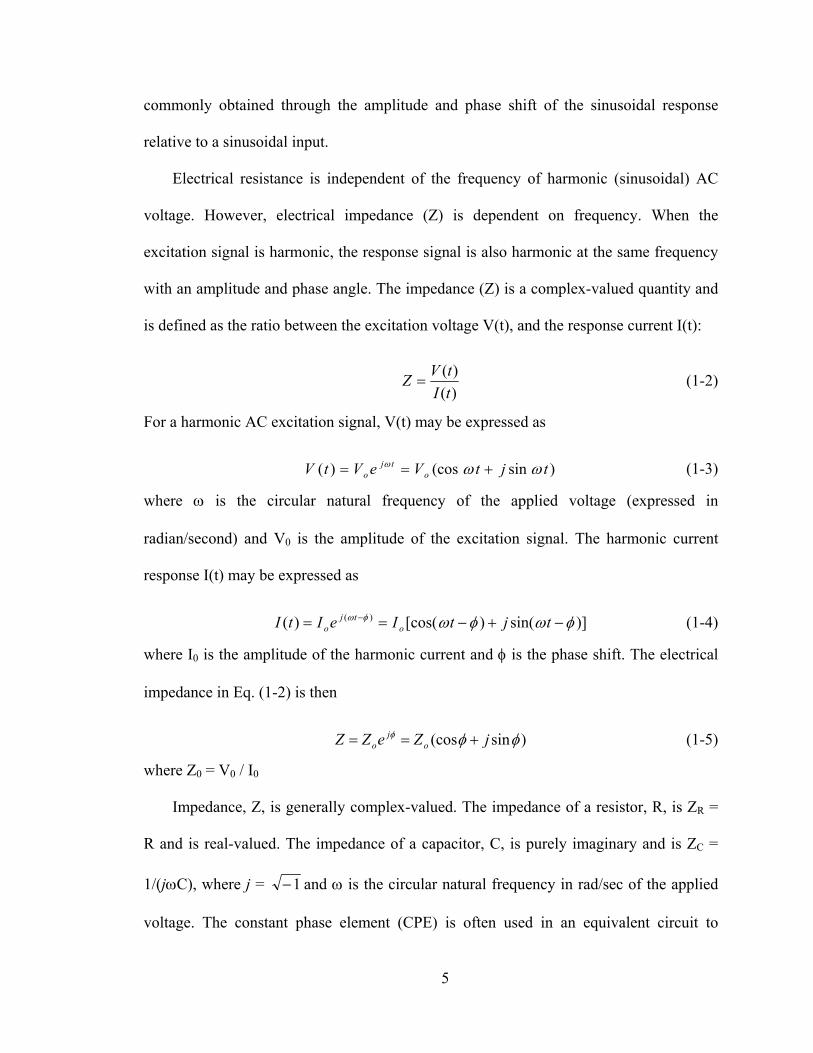
Electrical resistance is independent of the frequency of harmonic (sinusoidal) AC

voltage. However, electrical impedance (Z) is dependent on frequency. When the

excitation signal is harmonic, the response signal is also harmonic at the same frequency

with an amplitude and phase angle. The impedance (Z) is a complex-valued quantity and

is defined as the ratio between the excitation voltage V(t), and the response current I(t):

)()(

tItVZ = (1-2)

For a harmonic AC excitation signal, V(t) may be expressed as

(1-3) )sin(cos)( tjtVeVtV otj

o ωωω +==

where ω is the circular natural frequency of the applied voltage (expressed in

radian/second) and V0 is the amplitude of the excitation signal. The harmonic current

response I(t) may be expressed as

(1-4) )]sin()[cos()( )( φωφωφω −+−== − tjtIeItI otj

o

where I0 is the amplitude of the harmonic current and φ is the phase shift. The electrical

impedance in Eq. (1-2) is then

(1-5) )sin(cos φφφ jZeZZ oj

o +==

where Z0 = V0 / I0

Impedance, Z, is generally complex-valued. The impedance of a resistor, R, is ZR =

R and is real-valued. The impedance of a capacitor, C, is purely imaginary and is ZC =

1/(jωC), where j = 1− and ω is the circular natural frequency in rad/sec of the applied

voltage. The constant phase element (CPE) is often used in an equivalent circuit to

5

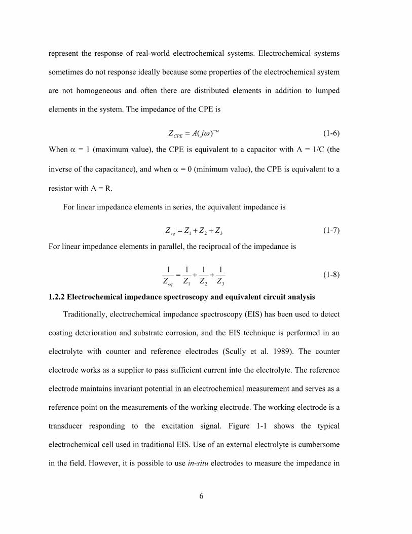
represent the response of real-world electrochemical systems. Electrochemical systems

sometimes do not response ideally because some properties of the electrochemical system

are not homogeneous and often there are distributed elements in addition to lumped

elements in the system. The impedance of the CPE is

(1-6) αω −= )( jAZCPE

When α = 1 (maximum value), the CPE is equivalent to a capacitor with A = 1/C (the

inverse of the capacitance), and when α = 0 (minimum value), the CPE is equivalent to a

resistor with A = R.

For linear impedance elements in series, the equivalent impedance is

321 ZZZZeq ++= (1-7)

For linear impedance elements in parallel, the reciprocal of the impedance is

321

1111ZZZZeq

++= (1-8)

1.2.2 Electrochemical impedance spectroscopy and equivalent circuit analysis

Traditionally, electrochemical impedance spectroscopy (EIS) has been used to detect

coating deterioration and substrate corrosion, and the EIS technique is performed in an

electrolyte with counter and reference electrodes (Scully et al. 1989). The counter

electrode works as a supplier to pass sufficient current into the electrolyte. The reference

electrode maintains invariant potential in an electrochemical measurement and serves as a

reference point on the measurements of the working electrode. The working electrode is a

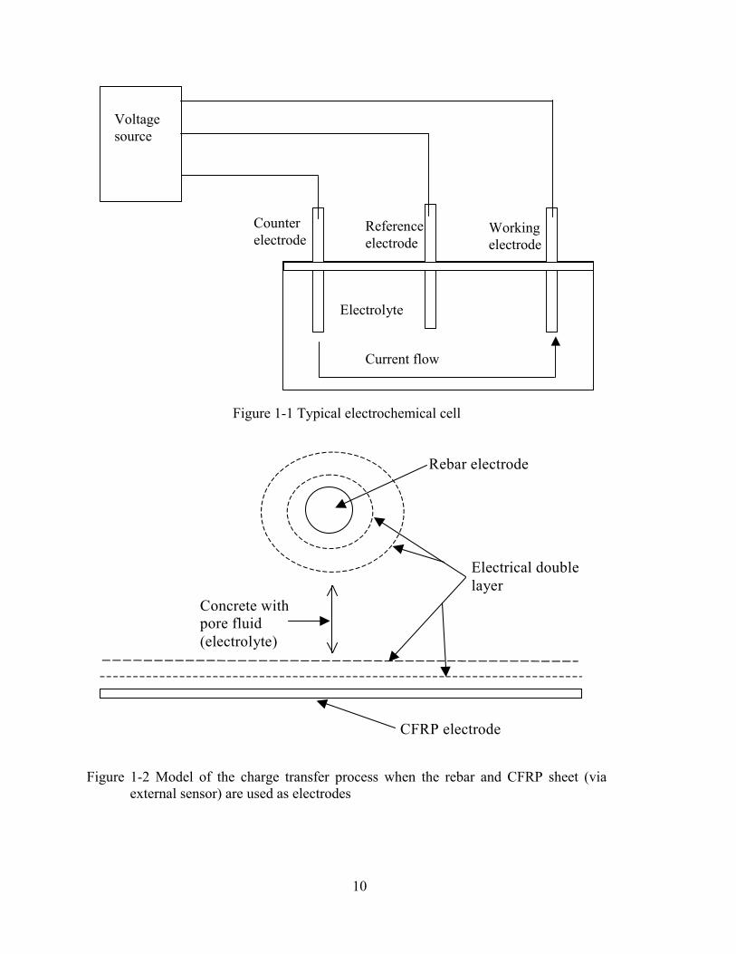
transducer responding to the excitation signal. Figure 1-1 shows the typical

electrochemical cell used in traditional EIS. Use of an external electrolyte is cumbersome

in the field. However, it is possible to use in-situ electrodes to measure the impedance in

6

the ambient condition without submerging the electrochemical cell using a modified EIS

technique (Davis et al. 2000).

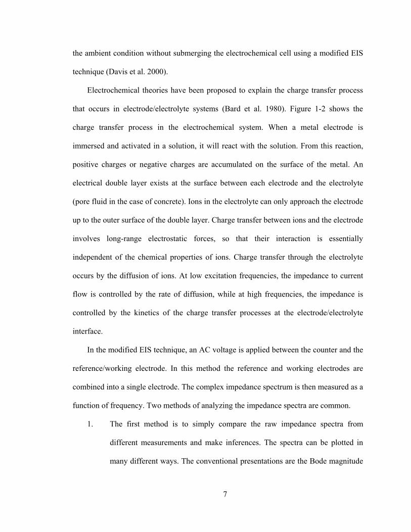
Electrochemical theories have been proposed to explain the charge transfer process

that occurs in electrode/electrolyte systems (Bard et al. 1980). Figure 1-2 shows the

charge transfer process in the electrochemical system. When a metal electrode is

immersed and activated in a solution, it will react with the solution. From this reaction,

positive charges or negative charges are accumulated on the surface of the metal. An

electrical double layer exists at the surface between each electrode and the electrolyte

(pore fluid in the case of concrete). Ions in the electrolyte can only approach the electrode

up to the outer surface of the double layer. Charge transfer between ions and the electrode

involves long-range electrostatic forces, so that their interaction is essentially

independent of the chemical properties of ions. Charge transfer through the electrolyte

occurs by the diffusion of ions. At low excitation frequencies, the impedance to current

flow is controlled by the rate of diffusion, while at high frequencies, the impedance is

controlled by the kinetics of the charge transfer processes at the electrode/electrolyte

interface.

In the modified EIS technique, an AC voltage is applied between the counter and the

reference/working electrode. In this method the reference and working electrodes are

combined into a single electrode. The complex impedance spectrum is then measured as a

function of frequency. Two methods of analyzing the impedance spectra are common.

1. The first method is to simply compare the raw impedance spectra from

different measurements and make inferences. The spectra can be plotted in

many different ways. The conventional presentations are the Bode magnitude

7

plot (log impedance magnitude vs log frequency), Bode phase angle plot

(phase angle vs log frequency), Nyquist plot (imaginary part of impedance vs

real part of impedance), real impedance plot (real parts of impedance vs log

frequency or log real parts of impedance vs log frequency), and imaginary

impedance plot (imaginary parts of impedance vs log frequency). The

magnitudes of impedance, phase angles, real impedances or imaginary

impedances are compared over the entire frequency range or over specific

frequency ranges.

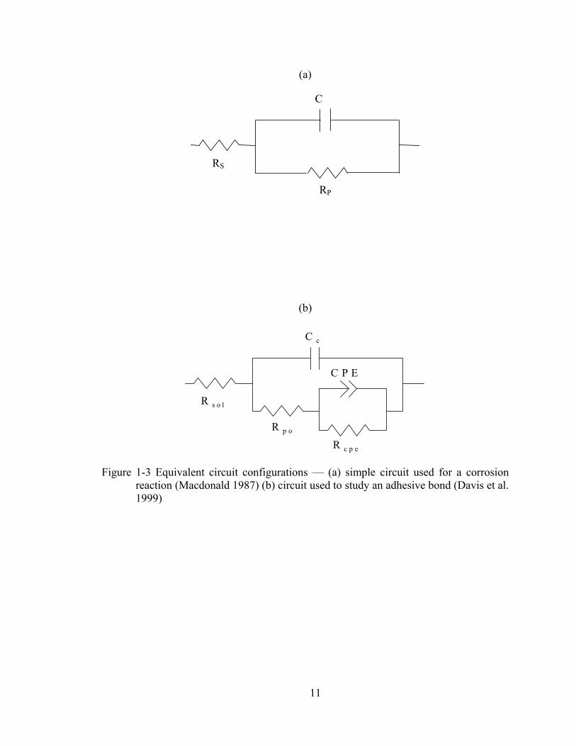
2. The second method is to analyze the impedance spectra by using an

equivalent circuit model. In this method, the parameters of an electrical circuit

which has a theoretical impedance similar to the measured impedance are

estimated, and spectra are compared based on the differences in the estimated

parameters. Typical equivalent circuits are shown in Figure 1-3. Figure 1-3

(a) shows a circuit used for corrosion studies (Macdonald 1987) and Figure

1-3 (b) shows the circuit used to study an adhesive bond (Davis et al. 1999).

Different equivalent circuits can be used to approximate a measured

impedance spectrum, and some experience is required to select an appropriate

circuit.

1.3 Use of EIS for Detection of Interfacial Degradation—A Literature Review

In-situ sensors have been adapted to detect moisture ingress and coating

deterioration. Davis et al. (1999) found a strong correlation between low frequency

impedance measurements and moisture ingress into coatings. They found that the initial

8

coating resistance was very high, but as the coating degrades due to moisture ingress, the

coating resistance decreases in the low frequency region.

An in-situ corrosion sensor previously used in monitoring coating degradation and

substrate corrosion of metals has been used to detect moisture ingress and crack

propagation in structural adhesive bonds. This sensor technology has also been used to

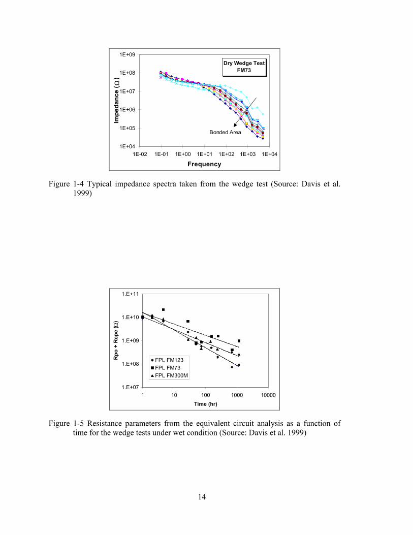
inspect the integrity of composite/composite bonds. Davis et al. (1999) conducted wedge

tests on bonded glass-reinforced and graphite-reinforced composites to assess the

integrity of the bond using EIS sensor technology. The wedge was driven into the

specimen until the two adherents separated and impedance measurements were taken.

The impedance typically increased in magnitude in the high-frequency region as the

crack propagated. Figure 1-4 shows the results of the wedge test.

9

Voltage source

Counter electrode

Reference electrode

Working electrode

Electrolyte

Current flow

Figure 1-1 Typical electrochemical cell

CFRP electrode

Concrete with pore fluid (electrolyte)

Rebar electrode

Electrical double layer

Figure 1-2 Model of the charge transfer process when the rebar and CFRP sheet (via external sensor) are used as electrodes

10

(a)

C

RS

RP

(b)

C c

R s o l

R p o

C P E

R c p e

Figure 1-3 Equivalent circuit configurations — (a) simple circuit used for a corrosion reaction (Macdonald 1987) (b) circuit used to study an adhesive bond (Davis et al. 1999)

11

In the simplest method for analyzing the debonding effects, the impedance spectra

can be compared directly (Figure 1-4). However, additional information can be obtained

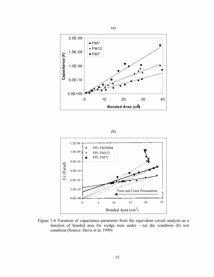
from the impedance spectra by using equivalent circuit analysis. Davis et al. (1999)

conducted the wedge tests under dry and wet conditions. They used the equivalent circuit

in Figure 1-3 (b), and found that the resistive components in the equivalent circuit they

used were functions of moisture content and the capacitance parameter was a function of

both moisture content and bonded area. The capacitance parameter from the equivalent

circuit analysis varied linearly with the bonded area in the dry wedge test. However, the

relationship was more complex when moisture was introduced during the wedge test. The

resistance parameters from the equivalent circuit analysis correlated with moisture level

in the electrochemical system. However, the resistance parameters did not show any

correlation with bonded area. Figures 1-5 and 1-6 show the correlations between the

parameters from the equivalent circuit analysis and the bonded area.

Davis et al. (1999) proposed the capacitance of an adhesive was influenced by the

dielectric constant of the adhesive, the thickness of the adhesive and the bonded area. The

capacitance may be expressed as

d

AC oεε= (1-9)

where C is the capacitance of the coating εo is the permitivity of free space, ε is the dielectric constant of the adhesive (which is dependant on the moisture content) A is the bonded area d is the thickness of the adhesive

The dielectric constant increases as moisture ingresses into the adhesive. The relationship

between the dielectric constant and moisture ingress is

12

)( AdWAd M εεεε −+= (1-10)

where εAd is the dielectric constant of the epoxy adhesive M is the moisture concentration in the adhesive εw is the dielectric constant of water

By combining Eq (1-9) and Eq. (1-10), the moisture increase in the adhesive from one

instart of measurement to another may be expressed as

−

∆=

AdW

Ad

ACM

εεε

α (1-11)

where ∆C is the difference between the measured capacitance at two

different times α is the slope of the dry capacitance vs bonded area relationship

13

Dry Wedge TestFM73

1E+04

1E+05

1E+06

1E+07

1E+08

1E+09

1E-02 1E-01 1E+00 1E+01 1E+02 1E+03 1E+04

Frequency

Impe

danc

e ( Ω

)

Bonded Area

Figure 1-4 Typical impedance spectra taken from the wedge test (Source: Davis et al. 1999)

1.E+07

1.E+08

1.E+09

1.E+10

1.E+11

1 10 100 1000 10000Time (hr)

Rpo

+ R

cpe

( Ω )

FPL FM123FPL FM73FPL FM300M

Figure 1-5 Resistance parameters from the equivalent circuit analysis as a function of time for the wedge tests under wet condition (Source: Davis et al. 1999)

14

(a)

0.0E+00

5.0E-10

1.0E-09

1.5E-09

2.0E-09

0 10 20 30 40 Bonded Area (cm2)

Cap

acita

nce

(F)

FM7FM12FM7

(b)

9 PL FM300M

FPL FM73 PL FM123

Cc

(Far

ad)

0

0

Tim rack Propagation

0

Figure 1-6 Vafunctioconditi

0.

Bonded Area (cm2)

rian on

to (

1.2E-0

i

1.0E-09

8.0E-10

6.0E-1

4.0E-1

2.0E-10

0E+0

on of f bondSource

0

capacitaned area : Davis e

5

ce paramfor wed

t al. 1999

10

eter fromge tests )

15

15

the equunder —

20

ivalent cir(a) dry c

25

FF

e and C

cuit analysis as a ondition (b) wet

1.4 Hypothesis and Objectives

The hypothesis investigated in this research is that EIS can be used to detect

debonding of CFRP reinforcement in concrete structures strengthened with CFRP. This

hypothesis is based on the successful use of this method for glass-reinforced

composite/composite bonds by Davis et al. (1999).

The objectives of the research are to:

• Develop effective sensor configurations, measurement schemes, and data

interpretation techniques.

• Ascertain the effects of short-term environmental conditions such as

temperature and humidity variations on the measurements and

interpretations.

• Ascertain the effect of long term environmental conditions such as freeze-

thaw cycles, wet-dry cycles and corrosion of reinforcement on the

measurements and interpretations

16

Chapter 2

Experimental Design

Debonding of external CFRP reinforcement was investigated by using wedge tests.

In these tests, the CFRP sheet is debonded by driving a thin wedge between it and the

concrete substrate. Impedance measurements are taken periodically and the variation of

impedance with the debonded length or area is studied.

Concrete structures rehabilitated with carbon fiber reinforced polymer (CFRP) are

subjected to various environmental conditions. The environmental conditions can be

divided into short-term and long-term conditions. Short-term environmental conditions

represent the conditions at the time impedance measurement are taken. These conditions

influence the impedance measurements, and include temperature variations, humidity

variations and variations in chloride concentration caused by deicing agents.. The long-

term environmental conditions include corrosion of reinforcing bars, freezing and

thawing cycles and wetting and drying cycles. The impact of short term and long term

environmental effects on impedance measurements must be well understood if the latter

are to be used to detect debonding of the CFRP. It also is important to have durable and

reliable sensors to obtain accurate impedance measurements during the service life time

of rehabilitated structures.

Three different humidity levels and three different temperatures were applied to six

reinforced-concrete specimens to study the sensitivity of sensor measurements on these

short term environmental conditions. Of the six specimens, three were manufactured with

chloride (18.6 lb NaCl per cubic yard of concrete) and three without chloride. Nine

17

reinforced concrete specimens with chloride were used to study the durability and

reliability of installed sensors. Three specimens were subjected to 300 freeze-thaw

cycles, three were subjected to 300 wet-dry cycles, and three were subjected to

accelerated corrosion conditions to study effects of rebar corrosion.

The size of the concrete specimens and the effective electrode area of installed

sensors can also affect impedance measurements. A large reinforced-concrete beam was

fabricated and used to study size effects.

2.1 Specimen Preparation and Sensor Configuration

2.1.1 Specimen sizes and preparation

Three different sizes of reinforced concrete beams were manufactured and used in

this research. Small reinforced-concrete prismatic beams (6 x 6 x 12 in.) with a #4

reinforcing bar were manufactured to study environmental effects on impedance

measurements. Medium reinforced concrete beams (6 x 6 x 24 in.) with a #4 reinforcing

bar were fabricated for conducting wedge tests to study the effect of CFRP debonding.

Each #4 reinforcing bar was installed near the bottom surface (1.5 in. up from the

bottom). A large reinforced concrete beam (1.5 x 2 x 8 ft) was fabricated to study the

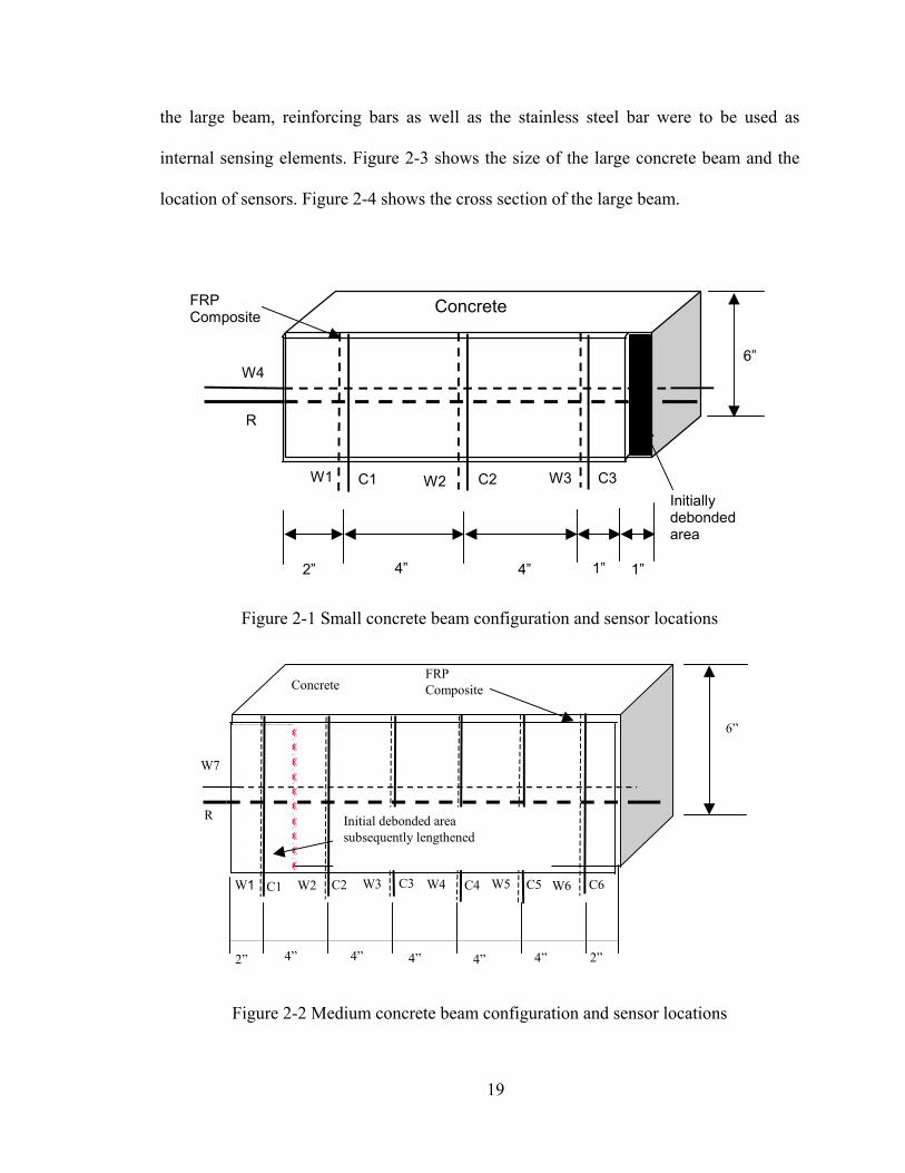
effect of CFRP debonding and specimen size. Figures 2-1 and 2-2 illustrate the size of the

concrete beams and the location of the reinforcing bar.

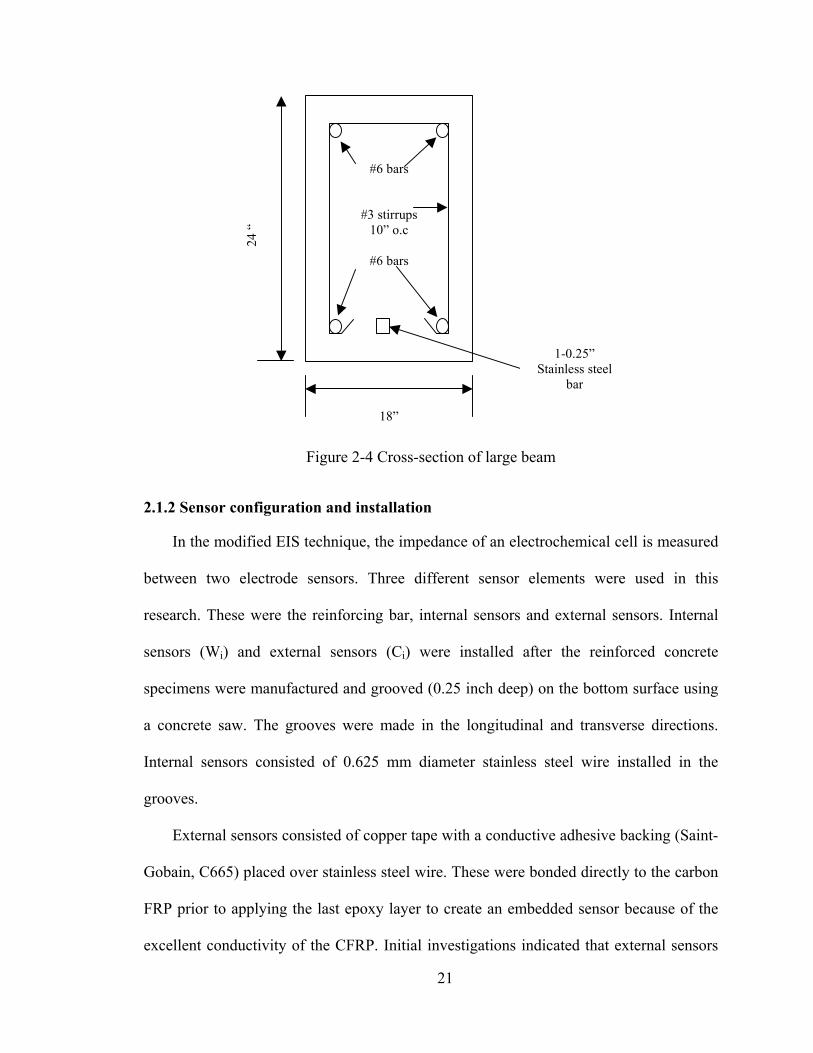
One large reinforced concrete beam of dimension 8’ x 1.5’ x 2’ was used to study

size effects. The concrete beam had four 8-foot long #6 bars, one 8-foot long quarter inch

by quarter inches square stainless steel bar, and number 3 stirrups at 10-inch spacing.

Reinforcing bars were planned to be used as internal sensing elements. The stainless steel

bar was included to eliminate the effect of corrosion which might affect measurements. In

18

the large beam, reinforcing bars as well as the stainless steel bar were to be used as

internal sensing elements. Figure 2-3 shows the size of the large concrete beam and the

location of sensors. Figure 2-4 shows the cross section of the large beam.

Concrete FRP Composite

W4

2”

R

4” 1”

W1 C1 W2 C3W3C2

6”

1”4”

Initially debonded area

Figure 2-1 Small concrete beam configuration and sensor locations

Concrete

FRP Composite

W1 W2 C2 C3 C1 W3 C4 W4 W5 C5 W6 C6

W7

R Initial debonded area subsequently lengthened

4” 4” 4” 4” 4” 2” 2”

6”

Figure 2-2 Medium concrete beam configuration and sensor locations

19

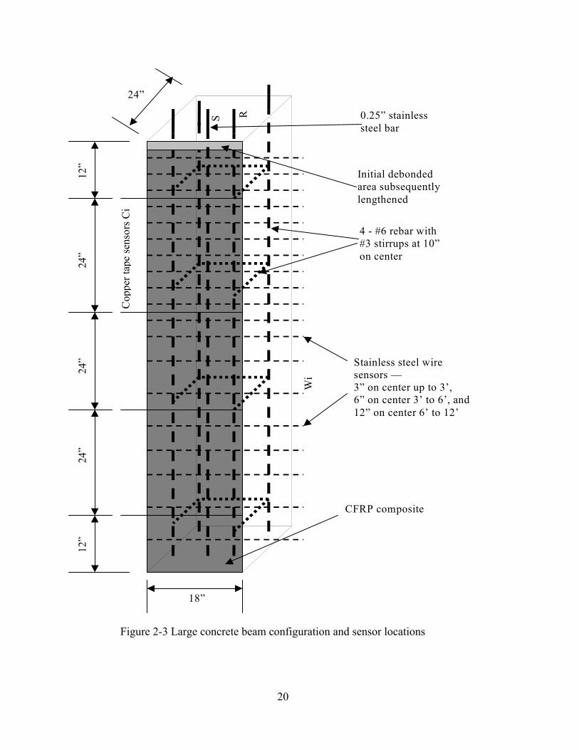
4 - #6 rebar with #3 stirrups at 10” on center

Initial debonded area subsequently lengthened

R

Stainless steel wire sensors — 3” on center up to 3’, 6” on center 3’ to 6’, and 12” on center 6’ to 12’

12”

24”

24”

24”

12”

18”

24”

CFRP composite

Wi

Cop

per t

ape

sens

ors C

i

S 0.25” stainless steel bar

Figure 2-3 Large concrete beam configuration and sensor locations

20

24 “

18”

1-0.25” Stainless steel

bar

#6 bars

#3 stirrups 10” o.c

#6 bars

Figure 2-4 Cross-section of large beam

2.1.2 Sensor configuration and installation

In the modified EIS technique, the impedance of an electrochemical cell is measured

between two electrode sensors. Three different sensor elements were used in this

research. These were the reinforcing bar, internal sensors and external sensors. Internal

sensors (Wi) and external sensors (Ci) were installed after the reinforced concrete

specimens were manufactured and grooved (0.25 inch deep) on the bottom surface using

a concrete saw. The grooves were made in the longitudinal and transverse directions.

Internal sensors consisted of 0.625 mm diameter stainless steel wire installed in the

grooves.

External sensors consisted of copper tape with a conductive adhesive backing (Saint-

Gobain, C665) placed over stainless steel wire. These were bonded directly to the carbon

FRP prior to applying the last epoxy layer to create an embedded sensor because of the

excellent conductivity of the CFRP. Initial investigations indicated that external sensors

21

applied to the outside of the CFRP after the final protective epoxy layer was applied were

ineffective. The thick protective epoxy layer yields impedances from the rebar to the

external sensors that are beyond the range of what can be measured with the Gamry

(PC4-300 Potentiostat board/11125) potentiostat. External sensors were installed only in

the transverse direction on the outmost surface of the CFRP reinforcement. The carbon

fibers are highly conductive in the longitudinal direction. However, because of gaps

between adjacent fibers, the conductivity in the lateral direction is generally poor. By

bonding the copper tape in the transverse direction across all the fibers in the carbon FRP,

good electrical contact can be made with the carbon fibers. The entire FRP then acts as

one of the electrodes in the cell. Since the copper tape is on the outside of the FRP, it

does not affect the bond between the FRP and the concrete or between different FRP

layers, and will therefore not compromise the strength of the CFRP reinforcement.

Figures 2-1, 2-2 and 2-3 show the configuration and direction of the sensors on the

concrete beam specimens. Table 2-1 shows the number of sensors and their directions.

For the large beam, the entire reinforcement cage (four longitudinal bars and stirrups)

acts as an internal sensors and the stainless steel bar was a second internal sensor.

Installation of internal sensors must be done carefully so that the stainless steel wires

do not touch the CFRP. A short circuit can be created between the copper tape on one

side of the CFRP and the wires on the other side. Even though there may be more than

one layer of CFRP used with a thin layer of epoxy between the layers, a short circuit can

be created. A heat-shrinking insulator was used around the internal sensors in the

transverse direction where they overlapped the internal sensors in the longitudinal

directions so that electrical contact between the wire electrodes was avoided. A heat-

22

shrinking insulator was also used on the internal sensors at the edge of the concrete

specimens to avoid contact with exposed carbon fiber in the CFRP. Field installation of

EIS sensors is described in Appendix B.

2.1.3 Sensor combinations for impedance measurements

Three different sensor combinations were used to measure the impedance.

Combinations of internal sensors (stainless steel wires Wi) to external sensors (copper

tapes Ci), rebar to external sensors, and internal sensors to internal sensors were used to

measure the raw impedance data. EIS measurements and interpretation are described in

Appendixes A and B.

Table 2-1 Number of sensors and their orientation on the specimens

Small size specimen Medium size specimen Large size specimen Transverse Longitudinal Transverse Longitudinal Transverse Longitudinal

Internal sensor 3 1 6 1 20 1

External sensor 3 0 6 0 4 0

Rebar 0 1 0 1 0 2

23

2.2 Detection of FRP Debonding

2.2.1 Two foot long specimens

Six 6”x 6” x 24” reinforced concrete specimens with chloride were prepared to

determine whether impedance measurements could be used to detect the debonding of

CFRP from concrete. Each specimen was prepared with an initial crack (4” in length)

between the CFRP and concrete using a teflon insert. To propagate the interfacial crack

between the CFRP sheet and the concrete substrate, a wedge (sharpened saw blade) was

driven with a hammer. The crack was propagated by two to four inches each time.

Impedance measurements were made at each extended crack states from the internal

sensors (stainless steel wire or reinforcing bar) to each of the copper tape sensors.

Investigation of the debonding of CFRP reinforcement from concrete was conducted

in two different environmental conditions. One was a controlled environment (in a

refrigerator) with a temperature of about 420F and a constant relative humidity level of

about 35% and the other was an ambient condition in the lab. It was noted during the

study on temperature effects that at high temperatures relatively small variations in

temperature caused significant variations in the impedance measurements. For this

reason, a cold temperature was chosen to reduce the sensitivity of the impedance

measurements to temperature fluctuations. Three concrete specimens were used in the

controlled environment. The ambient condition represented a temperature of about 700F

to 750F and a relative humidity that varied from 30% to 60%. Three concrete specimens

were subjected to the wedge test in the ambient condition.

24

2.2.2 Large beam specimen

The effective electrode area of installed sensors and the size of the concrete

specimen are expected to influence impedance measurements. Electrodes with larger

effective surface areas in the electrochemical cell typically decrease the magnitude of

impedance. A large reinforced-concrete beam was fabricated with external and internal

sensor to study the impact of specimen size. The large specimen was prepared with an

initial one-inch long crack by using a teflon insert. To create the interfacial crack between

the FRP layer and the concrete substrate, a sharpened metal sheet (wedge) was driven

with a hammer. The crack length was increased by two to four inches at each stage until

the crack length was about 25% of the length of the entire beam. Impedance

measurements were made at each extended crack state from internal sensors (stainless

steel wire, stainless steel bar or reinforcing bar) to each of the copper tape sensors and

between pairs of internal stainless steel wire sensors. The beam was constructed in the

laboratory and after 28 days of curing it was moved outdoors. The beam was exposed to

the winter climate from February 21 to April 2, 2003. The original intent was to conduct

the wedge test in an outdoor environment when temperatures were in the 35-450F range.

However, because of the unusually warm winter in 2003, temperature fluctuations were

large. After obtaining impedance measurements at one crack stage (three-inch long crack)

when the beam was outdoors, it was decided that the remainder of the test would be done

indoors. The wedge test was therefore conducted in a normal ambient condition at

temperatures between 650F and 750F and a relative humidity between 30% and 60%.

25

2.3 Assessment of the Sensitivity of Sensor Measurements to Environmental Effects

2.3.1 Humidity

Moisture in the concrete specimens is the medium for transporting charges between

sensors. Since charge is carried in the electrochemical cell (concrete specimen) by the

movement of ions, different levels of moisture should affect the capacity for transporting

charges. Three different humidity levels were considered in the study to assess the

sensitivity of sensor measurements to humidity.

Six small reinforced concrete specimens (6 x 6 x 12 in.) were subjected to relative

humidity levels of 30 percent, 60 percent and 90 percent in a controlled environmental

chamber, while the temperature was held constant at 720F (room temperature). The range

of relative humidities from 30 to 90 percent covers a wide range from extremely dry air

to highly saturated air.

Each of the six concrete specimens was subjected to the three different relative

humidity level, until the weight of the specimens stabilized. Of the six specimens, three

were manufactured with chloride (18.6 lb NaCl per cubic yard of concrete) and three

without chloride. Impedance measurements were taken after this exposure.

2.3.2 Temperature

Temperature affects the rate of ion transfer in electrolytes and is therefore expected

to influence the magnitude of impedance. In order to study temperature effects on the

impedance measurements, six small concrete specimens (6 x 6 x 12 in.) were subjected to

three different temperatures. The same six specimens used to study humidity effects were

reused. The specimens were subjected to extreme cold (temperature of about 00F), a

26

moderate temperature (about 700F) and a typical hot summer temperature (about 1000F).

The humidity level was not controlled. For the cold condition, the specimens were kept in

a freezer for a week at a temperature of 00F and the impedance measurements were taken

while specimens were inside the freezer. For the hot summer temperature, the specimens

were placed in an oven for a week at a temperature of 1000F and the impedance

measurements were taken while the specimens were inside the oven. For the moderate

temperature, specimens were exposed to a room temperature of 700F and a relative

humidity level of 60 percent.

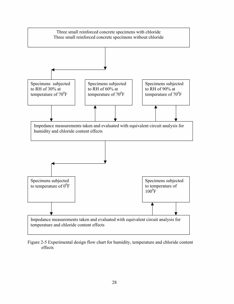
2.3.3 Chloride content

Chloride ions can exist in concrete structures from the time the concrete is cast due

to the use of chemical agents, and the concentration can change with time due to the

diffusion of deicing agents through the concrete. The existence of chloride ions in

concrete provides additional free ions for transport of charges in EIS and is expected to

have an effect on the measurements. An experiment was setup to study the sensitivity of

impedance measurements to the presence of chloride ions. The experiment to study

chloride effects was conducted simultaneously with the experiment to study humidity and

temperature effects. Six small reinforced concrete specimens (6 x 6 x12 in.) were used.

Of the six specimens, three were manufactured with chloride (18.6 lb NaCl per cubic

yard of concrete) and three without chloride. The specimens were subjected to relative

humidity levels of 30 percent, 60 percent and 90 percent at a temperature of 700 F in a

controlled environmental chamber and the same six reinforced concrete specimens were

also subjected to temperatures of 1000F and 00F without any humidity control. Figure 2-5

illustrates how the same specimens were re-used to study the effects of humidity,

temperature and chloride content.

27

Three small reinforced concrete specimens with chloride Three small reinforced concrete specimens without chloride

Impedance measurements taken and evaluated with equivalent circuit analysis for humidity and chloride content effects

Specimens subjected to RH of 60% at temperature of 700F

Specimens subjected to RH of 90% at temperature of 700F

Specimens subjected to RH of 30% at temperature of 700F

Specimens subjected to temperature of 1000F

Specimens subjected to temperature of 00F

Impedance measurements taken and evaluated with equivalent circuit analysis for temperature and chloride content effects

Figure 2-5 Experimental design flow chart for humidity, temperature and chloride content effects

28

2.3.4 Freeze – thaw

Concrete bridge structures in Michigan undergo freezing and thawing cycles in

winter which promotes the growth of microcracks in the concrete. This is likely to change

impedance measurements. A freeze-thaw test was setup to study the variability of sensor

measurements. This experiment was setup to determine the change in impedance

measurements before and after 300 freeze-thaw cycles. Three small concrete specimens

(6 x 6 x 12 in.) with chloride (18.6 lb NaCl per cubic yard of concrete) were used to study

freeze – thaw effects.

Initially, the concrete specimens were subjected to a temperature of about 700F and a

humidity level of 60 percent until their weight stabilized. The baseline impedance

measurements were then taken before the specimens were subjected to freeze-thaw

cycles. The specimens were then subjected to 300 cycles of freeze-thaw. The ASTM

C666 Procedure B was used in which each freeze –thaw cycle consisted of a two-hour

freezing period and a four-hour thawing period in a freeze-thaw machine. After 300

cycles of freeze-thaw, the specimens were removed from the freeze-thaw machine and

placed in an oven to dry out the excessive water absorbed during the freeze-thaw test.

Once the specimens reached approximately the same weight as before the freeze-thaw

test, they were conditioned at a temperature of about 700F and impedance measurements

were taken again.

2.3.5 Wetting and drying

Concrete bridge structures experience cycles of wetting and drying on a continuous

basis. The expansion and shrinkage resulting from wetting and drying cycles is likely to

promote the growth of microcracks and cause impedance measurements to change. A

wet-dry experiment was set up to study the changes in impedance measurements after

29

wet-dry cycles. Baseline impedance measurements were taken on three small concrete

specimens (6 x 6 x 12 in.) with chloride at a temperature of about 700F and a humidity

level of 60 percent. The specimens were then subjected to 300 wet-dry cycles. Each wet-

dry cycle consisted of a two hour wet period followed by a ten hour dry period. A 2%

NaCl solution was used to wet the specimens in order to increase the concentration of

chloride ions. After 300 cycles of wetting and drying, the specimens were placed in an

oven at a temperature of about 450C to dry out the excessive water absorbed during the

experiment. Once the concrete specimens reached approximately the same water content

at which the baseline measurement were taken, impedance measurements were retaken.

2.3.6 Corrosion of reinforcing bar

The reinforcing bar in the specimen was used as an internal sensor. The electrical

properties of the reinforcing bar and surrounding concrete may change due to corrosion

of the reinforcing bar and the presence of corrosion products in the concrete. Cracking of

the concrete surrounding the reinforcement due to the volume expansion associated with

corrosion also is likely to change impedance measurements. An accelerated corrosion

experiment was used to study the effect of corrosion of the reinforcing bar on the

impedance measurements.

For the corrosion study, small concrete specimens (6 x 6 x 12 in.) with two

reinforcing bars, one near the bottom face and the other near the top face, were used.

Baseline impedance measurements were taken at a temperature of 700F prior to the

accelerated corrosion test. A constant voltage of 12 V was then supplied across the two

reinforcing bars using an external power source. A 2 percent sodium chloride solution (by

weight) was used to wet the concrete specimens for one hour in each 24 hour period. The

moisture in the concrete specimens and the applied current induces corrosion in the

30

anodic reinforcing bar in an accelerated fashion. The anodic bar was located near the

bottom face of the specimens on which the CFRP was bonded. Figure 2-6 shows the

accelerated corrosion experimental setup. The three specimens were subjected to

accelerated corrosion for three weeks (21 days). The applied current was monitored at an

interval of two minutes with a voltage data-logging unit (Omega Engineering Inc.,

AD128-10T2), since this has a direct correlation with the total corrosion in the

reinforcing bar. After 21 days of accelerated corrosion, the specimens were placed in an

oven to dry out the excessive water absorbed during the wetting of the specimens.

Impedance measurements were taken once the concrete specimens reached

approximately the same water content at which the baseline measurement were taken.

31

R

R

External power source

+ –

Voltage data-logging unit

12Ω Resistor

Typical 6” x 6” x 12” specimen with two #4 reinforcing bar

CFRP sheet

12Ω Resistor

R

Figure 2-6 Experimental setup for accelerated corrosion

32

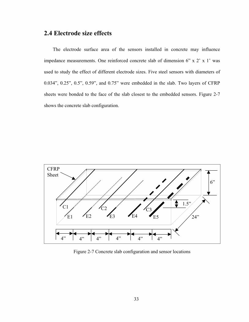
2.4 Electrode size effects

The electrode surface area of the sensors installed in concrete may influence

impedance measurements. One reinforced concrete slab of dimension 6” x 2’ x 1’ was

used to study the effect of different electrode sizes. Five steel sensors with diameters of

0.034”, 0.25”, 0.5”, 0.59”, and 0.75” were embedded in the slab. Two layers of CFRP

sheets were bonded to the face of the slab closest to the embedded sensors. Figure 2-7

shows the concrete slab configuration.

4” 4” 4” 4” 4” 4”

6”

24” E2 E1 E3C3C2C1

E5E4

1.5”

CFRP Sheet

Figure 2-7 Concrete slab configuration and sensor locations

33

34

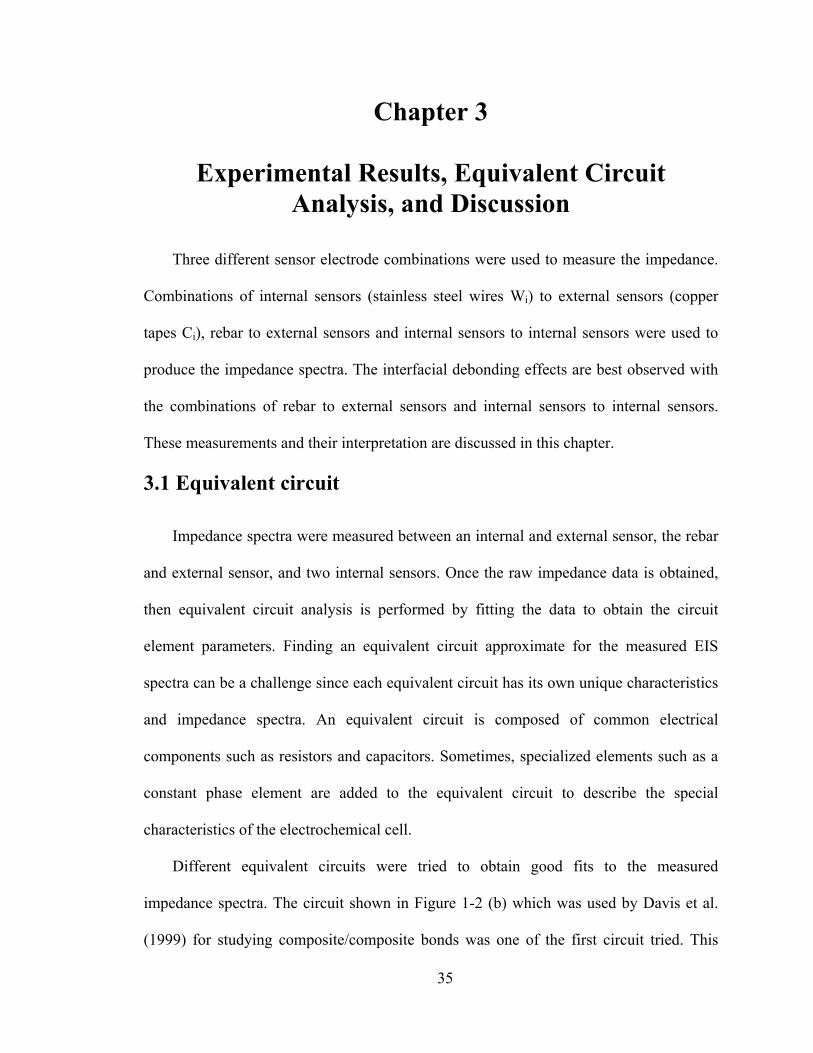
Chapter 3

Experimental Results, Equivalent Circuit Analysis, and Discussion

Three different sensor electrode combinations were used to measure the impedance.

Combinations of internal sensors (stainless steel wires Wi) to external sensors (copper

tapes Ci), rebar to external sensors and internal sensors to internal sensors were used to

produce the impedance spectra. The interfacial debonding effects are best observed with

the combinations of rebar to external sensors and internal sensors to internal sensors.

These measurements and their interpretation are discussed in this chapter.

3.1 Equivalent circuit

Impedance spectra were measured between an internal and external sensor, the rebar

and external sensor, and two internal sensors. Once the raw impedance data is obtained,

then equivalent circuit analysis is performed by fitting the data to obtain the circuit

element parameters. Finding an equivalent circuit approximate for the measured EIS

spectra can be a challenge since each equivalent circuit has its own unique characteristics

and impedance spectra. An equivalent circuit is composed of common electrical

components such as resistors and capacitors. Sometimes, specialized elements such as a

constant phase element are added to the equivalent circuit to describe the special

characteristics of the electrochemical cell.

Different equivalent circuits were tried to obtain good fits to the measured

impedance spectra. The circuit shown in Figure 1-2 (b) which was used by Davis et al.

(1999) for studying composite/composite bonds was one of the first circuit tried. This

35

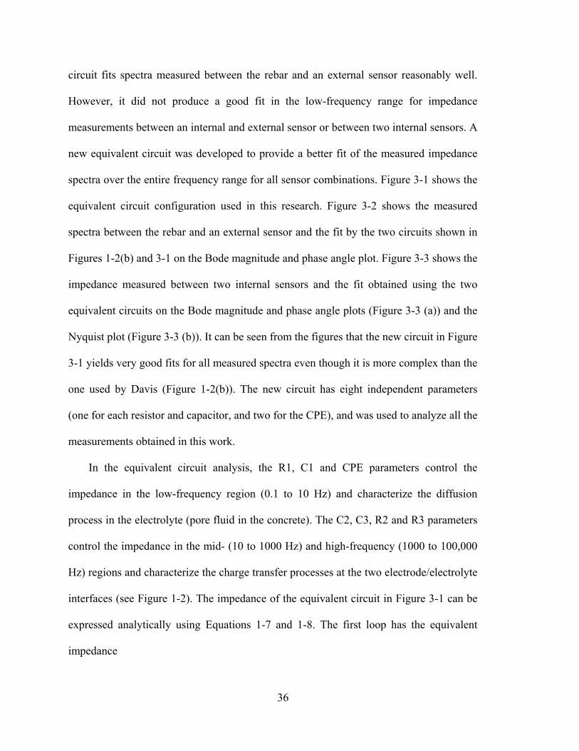
circuit fits spectra measured between the rebar and an external sensor reasonably well.

However, it did not produce a good fit in the low-frequency range for impedance

measurements between an internal and external sensor or between two internal sensors. A

new equivalent circuit was developed to provide a better fit of the measured impedance

spectra over the entire frequency range for all sensor combinations. Figure 3-1 shows the

equivalent circuit configuration used in this research. Figure 3-2 shows the measured

spectra between the rebar and an external sensor and the fit by the two circuits shown in

Figures 1-2(b) and 3-1 on the Bode magnitude and phase angle plot. Figure 3-3 shows the

impedance measured between two internal sensors and the fit obtained using the two

equivalent circuits on the Bode magnitude and phase angle plots (Figure 3-3 (a)) and the

Nyquist plot (Figure 3-3 (b)). It can be seen from the figures that the new circuit in Figure

3-1 yields very good fits for all measured spectra even though it is more complex than the

one used by Davis (Figure 1-2(b)). The new circuit has eight independent parameters

(one for each resistor and capacitor, and two for the CPE), and was used to analyze all the

measurements obtained in this work.

In the equivalent circuit analysis, the R1, C1 and CPE parameters control the

impedance in the low-frequency region (0.1 to 10 Hz) and characterize the diffusion

process in the electrolyte (pore fluid in the concrete). The C2, C3, R2 and R3 parameters

control the impedance in the mid- (10 to 1000 Hz) and high-frequency (1000 to 100,000

Hz) regions and characterize the charge transfer processes at the two electrode/electrolyte

interfaces (see Figure 1-2). The impedance of the equivalent circuit in Figure 3-1 can be

expressed analytically using Equations 1-7 and 1-8. The first loop has the equivalent

impedance

36

22221 QPYQSPj

QPSQPYZ

++

−++

= (3-1)

where

1)2

sin(**1* 1 += − απω αCAP

)2

cos(**1 απω α−+= ARY

)2

cos(**1**1*1 1 απωω α−+= CARCQ

)2

sin(** απω α−= AS

The second and third loops have the equivalent impedances

222

2

2222 2*2*12*2*

2*2*12

RCRCj

RCRZ

ωω

ω +−

+= (3-2)

222

2

2223 3*3*13*3*

3*3*13

RCRCj

RCRZ

ωω

ω +−

+= (3-3)

The impedance of the entire circuit is therefore

321 ZZZZeq ++= (3-4)

37

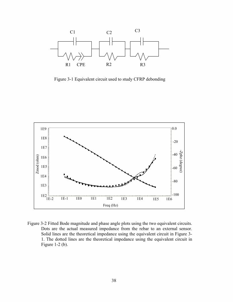
C1

R1 CPE R3

C3

R2

C2

Figure 3-1 Equivalent circuit used to study CFRP debonding

1E9

1E8

1E7

1E6

1E5

1E4

1E3

1E2 1E-2 1E3 1E4 1E5 1E6 1E-1 1E0 1E1

0.0

-20

-60

-40

1E2-100

-80

Zmod

(ohm

)

Freq (Hz)

-Zphz (degree)

Figure 3-2 Fitted Bode magnitude and phase angle plots using the two equivalent circuits. Dots are the actual measured impedance from the rebar to an external sensor. Solid lines are the theoretical impedance using the equivalent circuit in Figure 3-1. The dotted lines are the theoretical impedance using the equivalent circuit in Figure 1-2 (b).

38

(a)

(b)

1E7

1E6

1EZmod

(ohm

)

-80

4E6

2.5E6

1.5E6

1.0E6

0.0

2.0E6

0.5E6

0.0 3E6 5E6 1E6 2E6

-Zim

ag (o

hm)

Zreal (ohm)

5

1E4 1E01E-2 1E3 1E4 1E5 1E6 1E-1 1E1

0.0

-20

-60

-40

1E2-100

Freq (Hz)

-Zphz (degree)

Figure 3-3 Fitting with the equivalent circuits. Dots are the actual measured impedances between two internal sensors. Solid lines are the theoretical impedances using the equivalent circuit in Figure 3-1. The dotted lines are the theoretical impedances using the equivalent circuit in Figure 1-2 (b). — (a) Bode magnitude and phase angle plot; (b) Nyquist plot.

39

3.2 CFRP Debonding

3.2.1 Results for 2-foot long specimens

Based on measurements from numerous pairs of sensors, it was found that

measurements from the rebar to external sensors had the strongest promise for revealing a

relationship between impedance measurements and the debonded area of CFRP. Figures

3-4 and 3-5 show the effect of CFRP debonding on the magnitude of the measured

impedance in the controlled environment (in the refrigerator), and in the uncontrolled

environment (ambient condition), respectively. These figures show that the measured

impedance increases over all frequencies due to debonding of the CFRP. The effects of

CFRP debonding on the measured impedance in the controlled environment also can be

seen with the Nyquist plot in Figure 3-6. The radius of the arc in the Nyquist plot

increases as the crack length increases. Figure 3-7 is an enlargement of Figure 3-5 in the

low- to mid-frequency range and shows the interference of humidity and debonding

effects on the measured impedance. The ambient relative humidity fluctuated from 30%

to 60% when the crack lengths increased from 6 in. to 10 in. This increase in relative

humidity caused the impedance magnitude at low frequencies to decrease even though

the interfacial crack length increased. However, the increase in humidity did not cause a

reversal in the measured impedance at mid- and high- frequencies. The interference of

humidity and debonding effects on the measured impedance can be seen more clearly on

the Nyquist plot shown in Figure 3-8. The radii of the arc in the Nyquist plot decreased

significantly when the crack lengths were at 8 and 10 inches.

40

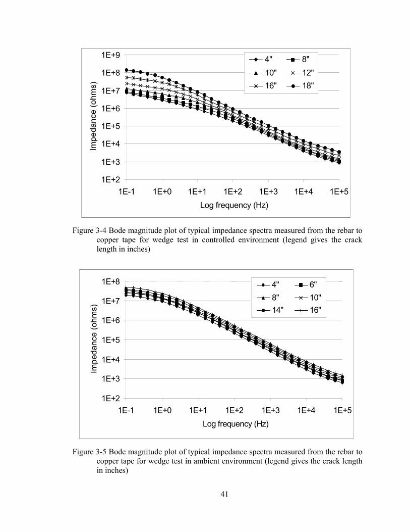
1E+2

1E+3

1E+4

1E+5

1E+6

1E+7

1E+8

1E+9

1E-1 1E+0 1E+1 1E+2 1E+3 1E+4 1E+5 Log frequency (Hz)

Impe

danc

e (o

hms)

4" 8" 10" 12" 16" 18"

Figure 3-4 Bode magnitude plot of typical impedance spectra measured from the rebar to copper tape for wedge test in controlled environment (legend gives the crack length in inches)

1E+2

1E+3

1E+4

1E+5

1E+6

1E+7

1E+8

1E-1 1E+0 1E+1 1E+2 1E+3 1E+4 1E+5Log frequency (Hz)

Impe

danc

e (o

hms)

4" 6" 8" 10" 14" 16"

Figure 3-5 Bode magnitude plot of typical impedance spectra measured from the rebar to copper tape for wedge test in ambient environment (legend gives the crack length in inches)

41

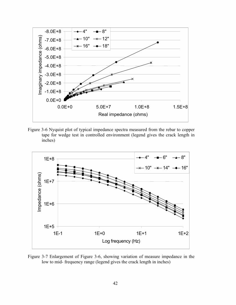
-8.0E+8

-7.0E+8

-6.0E+8

-5.0E+8

-4.0E+8

-3.0E+8

-2.0E+8

-1.0E+8

0.0E+0 0.0E+0 5.0E+7 1.0E+8 1.5E+8

Real impedance (ohms)

Imag

inar

y im

peda

nce

(ohm

s) 4" 8"

10" 12" 16" 18"

Figure 3-6 Nyquist plot of typical impedance spectra measured from the rebar to copper tape for wedge test in controlled environment (legend gives the crack length in inches)

1E+5

1E+6

1E+7

1E+8

1E-1 1E+0 1E+1 1E+2 Log frequency (Hz)

Impe

danc

e (o

hms)

4" 6" 8"

10" 14" 16"

Figure 3-7 Enlargement of Figure 3-6, showing variation of measure impedance in the low to mid- frequency range (legend gives the crack length in inches)

42

-2.5E+7

-2.0E+7

-1.5E+7

-1.0E+7

-5.0E+6

0.0E+0 0.0E+0 1.0E+7 2.0E+7 3.0E+7 4.0E+7 5.0E+7 6.0E+7

Real impedance (ohms)

Imag

inar

y im

peda

nce

(ohm

s) 4"

6"

8"

10"

14"

16"

Figure 3-8 Nyquist plot of impedance spectra measured from the rebar to copper tape for wedge test in ambient environment (legend gives the crack length in inches)

43

3.2.1.1 Comparison of raw impedance spectra

Figures 3-9 to 3-11 show the variation of the measured impedance at 10,000 Hz, 100

Hz and 1 Hz as a function of the interfacial crack length. These frequencies are arbitrary

representative of high, medium and low frequencies. The impedance magnitude vs. crack

length curves are close together at 10,000 Hz, and spread further and further apart at 100

Hz and 1 Hz. The specimen-to-specimen variation in the measurements is therefore the

least at high frequencies. In general, the measured impedance at a specific frequency

increases exponentially as the crack length increases.

3.2.1.2 Results from equivalent circuit analysis

The variation of the CPE parameter with crack length is shown in Figures 3-12 and

3-13. Although the CPE parameter exhibits good correlation with the interfacial crack

length it has high specimen-to-specimen variation and is also sensitive to temperature and

humidity. The variations of the capacitance parameters with interfacial crack length are

shown in Figures 3-14 to 3-16. The capacitance parameters exhibit a linear relation with

the crack length and except for specimen 3, the C2+C3 and C1+C2+C3 values for the

other four specimens are quite similar.

44

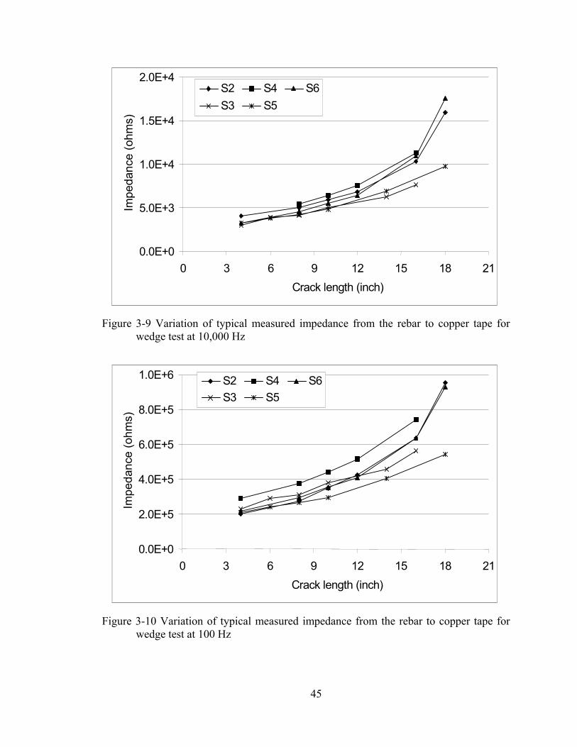
0.0E+0

5.0E+3

1.0E+4

1.5E+4

2.0E+4

0 3 6 9 12 15 18 21Crack length (inch)

Impe

danc

e (o

hms)

S2 S4 S6 S3 S5

Figure 3-9 Variation of typical measured impedance from the rebar to copper tape for wedge test at 10,000 Hz

0.0E+0

2.0E+5

4.0E+5

6.0E+5

8.0E+5

1.0E+6

0 3 6 9 12 15 18 21Crack length (inch)

Impe

danc

e (o

hms)

S2 S4 S6 S3 S5

Figure 3-10 Variation of typical measured impedance from the rebar to copper tape for wedge test at 100 Hz

45

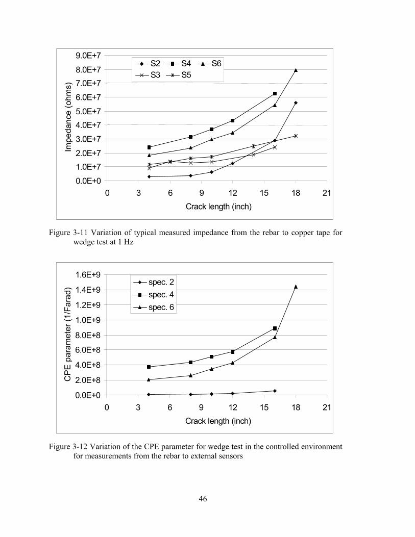
0.0E+0

1.0E+7 2.0E+7

3.0E+7

4.0E+7 5.0E+7

6.0E+7

7.0E+7 8.0E+7

9.0E+7

0 3 6 9 12 15 18 21 Crack length (inch)

Impe

danc

e (o

hms)

S2 S4 S6 S3 S5

Figure 3-11 Variation of typical measured impedance from the rebar to copper tape for wedge test at 1 Hz

0.0E+0

2.0E+8

4.0E+8

6.0E+8

8.0E+8

1.0E+9

1.2E+9

1.4E+9

1.6E+9

0 3 6 9 12 15 18 21 Crack length (inch)

CP

E p

aram

eter

(1/F

arad

) spec. 2spec. 4spec. 6

Figure 3-12 Variation of the CPE parameter for wedge test in the controlled environment for measurements from the rebar to external sensors

46

0.0E+0

2.0E+7

4.0E+7

6.0E+7

8.0E+7

1.0E+8

1.2E+8

0 3 6 9 12 15 18 21Crack length (inch)

CP

E p

aram

eter

(1/F

arad

) spec. 2spec. 3spec. 5

Figure 3-13 Variation of the CPE parameter for wedge test in ambient condition for measurements from the rebar to external sensors (Note: the CPE parameter for spec. 2 is measured in controlled environment)

0.0E+0

1.0E-9

2.0E-9

3.0E-9

4.0E-9

5.0E-9

6.0E-9

7.0E-9

8.0E-9

0 3 6 9 12 15 18 21Crack length (inch)

C1

para

met

er (F

arad

)

spec. 2 spec. 3spec. 4 spec. 5spec. 6

Figure 3-14 Variation of the C1 parameter from equivalent circuit analysis for wedge test from the rebar to external sensors

47

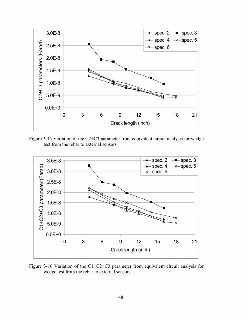
0.0E+0

5.0E-9

1.0E-8

1.5E-8

2.0E-8

2.5E-8

3.0E-8

0 3 6 9 12 15 18 21 Crack length (inch)

C2+

C3

para

met

ers

(Far

ad)

spec. 2 spec. 3 spec. 4 spec. 5 spec. 6

Figure 3-15 Variation of the C2+C3 parameter from equivalent circuit analysis for wedge test from the rebar to external sensors

0.0E+0

5.0E-9

1.0E-8

1.5E-8

2.0E-8

2.5E-8

3.0E-8

3.5E-8

0 3 6 9 12 15 18 21 Crack length (inch)

C1+

C2+

C3

para

met

er (F

arad

)

spec. 2 spec. 3 spec. 4 spec. 5 spec. 6

Figure 3-16 Variation of the C1+C2+C3 parameter from equivalent circuit analysis for wedge test from the rebar to external sensors

48

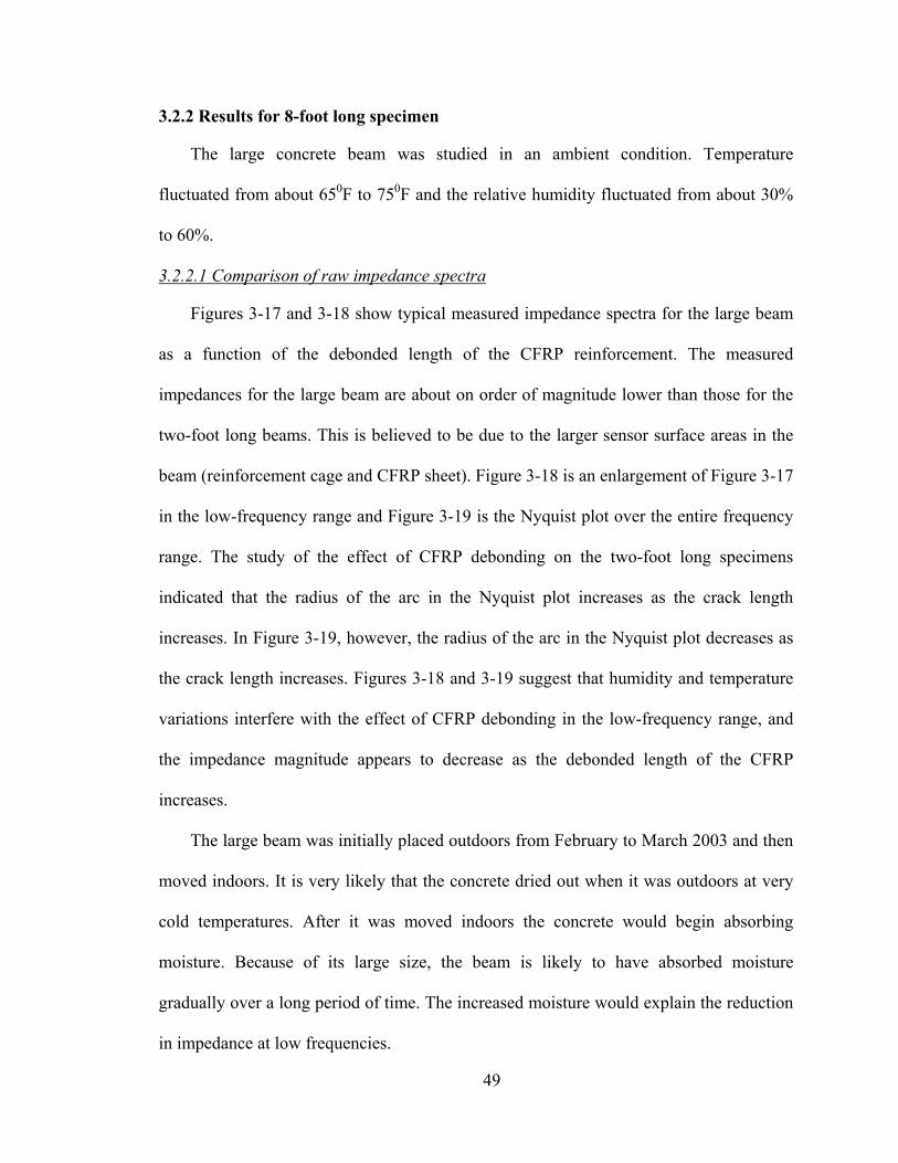
3.2.2 Results for 8-foot long specimen

The large concrete beam was studied in an ambient condition. Temperature

fluctuated from about 650F to 750F and the relative humidity fluctuated from about 30%

to 60%.

3.2.2.1 Comparison of raw impedance spectra

Figures 3-17 and 3-18 show typical measured impedance spectra for the large beam

as a function of the debonded length of the CFRP reinforcement. The measured

impedances for the large beam are about on order of magnitude lower than those for the

two-foot long beams. This is believed to be due to the larger sensor surface areas in the

beam (reinforcement cage and CFRP sheet). Figure 3-18 is an enlargement of Figure 3-17

in the low-frequency range and Figure 3-19 is the Nyquist plot over the entire frequency

range. The study of the effect of CFRP debonding on the two-foot long specimens

indicated that the radius of the arc in the Nyquist plot increases as the crack length

increases. In Figure 3-19, however, the radius of the arc in the Nyquist plot decreases as

the crack length increases. Figures 3-18 and 3-19 suggest that humidity and temperature

variations interfere with the effect of CFRP debonding in the low-frequency range, and

the impedance magnitude appears to decrease as the debonded length of the CFRP

increases.

The large beam was initially placed outdoors from February to March 2003 and then

moved indoors. It is very likely that the concrete dried out when it was outdoors at very

cold temperatures. After it was moved indoors the concrete would begin absorbing

moisture. Because of its large size, the beam is likely to have absorbed moisture

gradually over a long period of time. The increased moisture would explain the reduction

in impedance at low frequencies.

49

Figure 3-20 is an enlargement of Figure 3-17 in the high-frequency range. In the high

frequency range the magnitude of the impedance increases with the debonded length of

the CFRP although humidity and temperature fluctuated. Figure 3-21 shows typical

measured impedance spectra from the rebar and the stainless steel bar to copper tape

sensor. The measured impedance spectra from the stainless steel bar were very similar to

the measurements from the rebar. Figure 3-22 shows the measured impedance at 100,000

Hz. At this frequency the impedance magnitude shows a linear relation with the

debonded length of CFRP.

3.2.2.2 Results from equivalent circuit analysis

Figures 3-23 and 3-24 show the variation of the parameters from the equivalent

circuit analysis due to CFRP debonding. The CPE parameter decreased as the crack was

propagated. This is a direct result of the low–frequency behavior of the impedance

(Figure 3-19) and is opposite to what is expected. The C1 parameter was almost constant

during the CFRP debonding test. It is speculated that the effect of CFRP debonding on

the C1 parameter was compensated by variations in humidity and temperature. The

C2+C3 parameter and the C1+C2+C3 parameters decreased significantly during the

initial debonding of the CFRP.

50

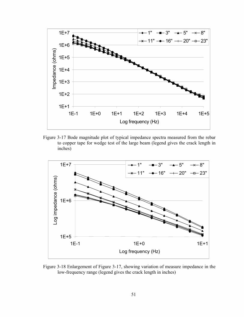
1E+1

1E+2

1E+3

1E+4

1E+5

1E+6

1E+7

1E-1 1E+0 1E+1 1E+2 1E+3 1E+4 1E+5Log frequency (Hz)

Impe

danc

e (o

hms)

1" 3" 5" 8" 11" 16" 20" 23"

Figure 3-17 Bode magnitude plot of typical impedance spectra measured from the rebar to copper tape for wedge test of the large beam (legend gives the crack length in inches)

1E+5

1E+6

1E+7

1E-1 1E+0 1E+1 Log frequency (Hz)

Log

impe

danc

e (o

hms)

1" 3" 5" 8"

11" 16" 20" 23"

Figure 3-18 Enlargement of Figure 3-17, showing variation of measure impedance in the low-frequency range (legend gives the crack length in inches)

51

-6.0E+6

-5.0E+6

-4.0E+6

-3.0E+6

-2.0E+6

-1.0E+6

0.0E+0 0.0E+0 5.0E+5 1.0E+6 1.5E+6 2.0E+6 2.5E+6 3.0E+6

Real impedance (ohms)

Imag

inar

y im

peda

nce

(ohm

s) 1" 3" 5" 8"

11" 16" 20" 23"

Figure 3-19 Nyquist plot of impedance spectra measured from the rebar to copper tape for wedge test of large beam in ambient environment (legend gives the crack length in inches)

1.0E+1

6.0E+1

1.1E+2

1.6E+2

2.1E+2

2.6E+2

3.1E+2

3.6E+2 4.1E+2

1E+4 1E+5 Log frequency (Hz)

Mag

nitu

de o

f im

peda

nce

(ohm

s) 1" 3" 5"

8" 11" 16" 20" 23"

Figure 3-20 Enlargement of Figure 3-17 showing variation of measured impedance in the high-frequency range (legend gives the crack length in inches)

52

1E+1

1E+2

1E+3

1E+4

1E+5

1E+6

1E+7

1E-1 1E+0 1E+1 1E+2 1E+3 1E+4 1E+5 Log frequency (Hz)

Log

impe

danc

e (o

hms)

Rebar

Stainless steel bar

Figure 3-21 Bode magnitude plot of typical impedance spectra measured from the rebar to copper tape and the stainless steel bar to copper tape for wedge test of the large beam (legend gives the crack length in inches)

0

10

20

30

40

50

60

70

80

0 3 6 9 12 15 18 21 24 Crack length (inch)

Mag

nitu

de o

f im

peda

nce

(ohm

s)

Figure 3-22 Variation of typical measured impedance from the rebar to copper tape for wedge test at 100,000 Hz

53

0.0E+0

1.0E+6

2.0E+6

3.0E+6

4.0E+6

5.0E+6

6.0E+6

0 3 6 9 12 15 18 21 24 Crack length (inch)

CP

E p

aram

eter

(1/F

arad

)

Figure 3-23 Variation of the CPE parameter from equivalent circuit analysis for the large specimen from the rebar to external sensor

0.0E+0 2.0E-8 4.0E-8 6.0E-8 8.0E-8 1.0E-7 1.2E-7 1.4E-7 1.6E-7 1.8E-7 2.0E-7

0 3 6 9 12 15 18 21 24 Crack length (inch)

Cap

acita

nce

para

met

er(F

arad

) C1 C2+C3 C1+C2+C3

Figure 3-24 Variation of the capacitance parameters from equivalent circuit analysis for the large specimen from the rebar to external sensor

54

3.2.3 Detecting the location of debonded regions

While impedance measurements between the rebar and an external sensor provide a

global assessment of the debonded area, they are incapable of revealing the location of

debonded regions. However, impedance measurements between pairs of internal wire

sensors (Wi) can be used to detect debonded regions. Measurements between internal

sensors were taken for the large eight-foot long beam as well as for a two-foot long

specimen as the internal crack between the CFRP and concrete was propagated.

3.2.3.1 Comparison of raw impedance spectra

Impedance measurements were made between adjacent sensors (such as W1 and W2,

W2 and W3, and so on). Figures 3-25 to 3-28 show the variation of measured impedance

at different crack states. Figure 3-25 shows the measured impedance from the eight-foot

long specimen when the crack between the CFRP and concrete was about 8 inches long

with the crack tip between sensors W2 and W3. At this crack length, W1 and W2 were in

the debonded region and the remaining sensors were in the bonded region. The measured

impedance between sensors in the debonded region (W1W2) had the highest magnitude

especially in the low-frequency region. The measured impedances between sensors in the

bonded region (W3W4, W4W5, and W5W6) had the lowest magnitudes. The same

distinguishable trends on the impedance measurements were observed with a two-foot

long specimen. Figure 3-26 shows the measured impedance from two-foot long specimen

when the crack was about 12 inches long with the crack tip between sensor W3 and W4.

At this crack length, W1, W2, and W3 were in the debonded region and W4, W5, and W6

were in the bonded region.

Measured impedances between a sensor in the debonded region and a sensor in the

bonded region (eg., W1W4 and W2W3 from Figure 3-25 and W3W4 from Figure 3-26)

55

have magnitudes that fall inbetween those corresponding to sensors in the debonded

region and those corresponding to sensors in the bonded region. Figure 3-27 shows the

Nyquist plot corresponding to Figure 3-26. On the Nyquist plot, the impedance

measurements from the sensors in the debonded region yield the largest arc radii while

the impedance measurements from the sensors in the bonded region produce the smallest

arc radii. When one sensor is in the bonded region and the other in the debonded region

(W3W4), the arc radii is in between those for the other two cases.

Figure 3-28 shows the measured impedances for the two-foot long specimen when

the CFRP was debonded to 16 inches with the crack tip between the W5 and W6 sensors.

Again, impedance magnitudes between sensors in the debonded region (W1W2, W2W3,

W3W4, and W4W5) are much higher than those in the bonded region (W6W7, W7W8,

and W8W9), especially at low frequencies.

56

1E+4

1E+5

1E+6

1E+7

1E+8

1E+9

1E-1 1E+0 1E+1 1E+2 1E+3 1E+4 1E+5 Log frequency (Hz)

Log

impe

danc

e (o

hms)

W1W2 W1W4

W2W3 W3W4

W4W5 W5W6

Figure 3-25 Bode magnitude plot of impedance spectra measured between pairs of internal sensors for eight-foot specimen in ambient condition when crack tip was between sensors W2 and W3 (legend shows the internal sensors used)

1E+5

1E+6

1E+7

1E+8

1E+9

1E+10

1E-1 1E+0 1E+1 1E+2 1E+3 1E+4 1E+5Log frequecy (Hz)

Log

impe

danc

e (o

hms)

w1w2 w2w3w3w4 w4w5w5w6

Figure 3-26 Bode magnitude plot of impedance spectra measured between pairs of internal sensors for two-foot specimen in ambient condition when crack tip was between sensors W3 and W4 (legend shows the internal sensors used)

57

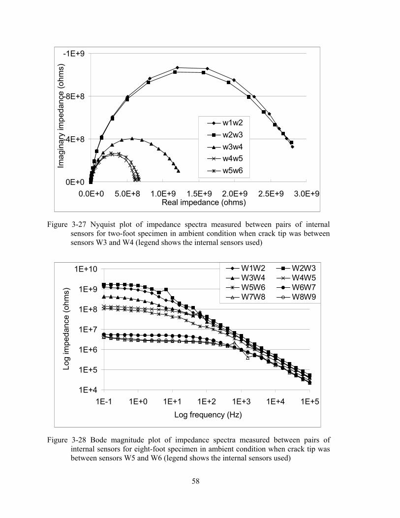
-1E+9

-8E+8

-4E+8

0E+0 0.0E+0 5.0E+8 1.0E+9 1.5E+9 2.0E+9 2.5E+9 3.0E+9

Real impedance (ohms)

Imag

inar

y im

peda

nce

(ohm

s)

w1w2w2w3w3w4w4w5w5w6

Figure 3-27 Nyquist plot of impedance spectra measured between pairs of internal sensors for two-foot specimen in ambient condition when crack tip was between sensors W3 and W4 (legend shows the internal sensors used)

1E+4

1E+5

1E+6

1E+7

1E+8

1E+9

1E+10

1E-1 1E+0 1E+1 1E+2 1E+3 1E+4 1E+5 Log frequency (Hz)

Log

impe

danc

e (o

hms)

W1W2 W2W3 W3W4 W4W5 W5W6 W6W7 W7W8 W8W9

Figure 3-28 Bode magnitude plot of impedance spectra measured between pairs of internal sensors for eight-foot specimen in ambient condition when crack tip was between sensors W5 and W6 (legend shows the internal sensors used)

58

3.2.3.2 Results from equivalent circuit analysis

While raw impedance measurements are sufficient to detect debonded regions,

equivalent circuit analysis also can be used. The effect of debonding on the impedances

measured between internal sensors is best observed with the CPE parameter which

characterizes the low-frequency behavior of the impedance spectrum. The variation of the

CPE values corresponding to the spectra in Figure 3-25 are shown in Figure 3-29 (crack

tip was between the W2 and W3 sensors). Figure 3-30 shows the variation of the CPE

values corresponding to the spectra in Figure 3-26 (crack tip between the W3 and W4

sensors). The magnitude of the CPE parameter corresponding to measurements between

pairs of sensors in the debonded region are about two orders of magnitude higher than

those corresponding to pairs of sensors in the bonded region.

59

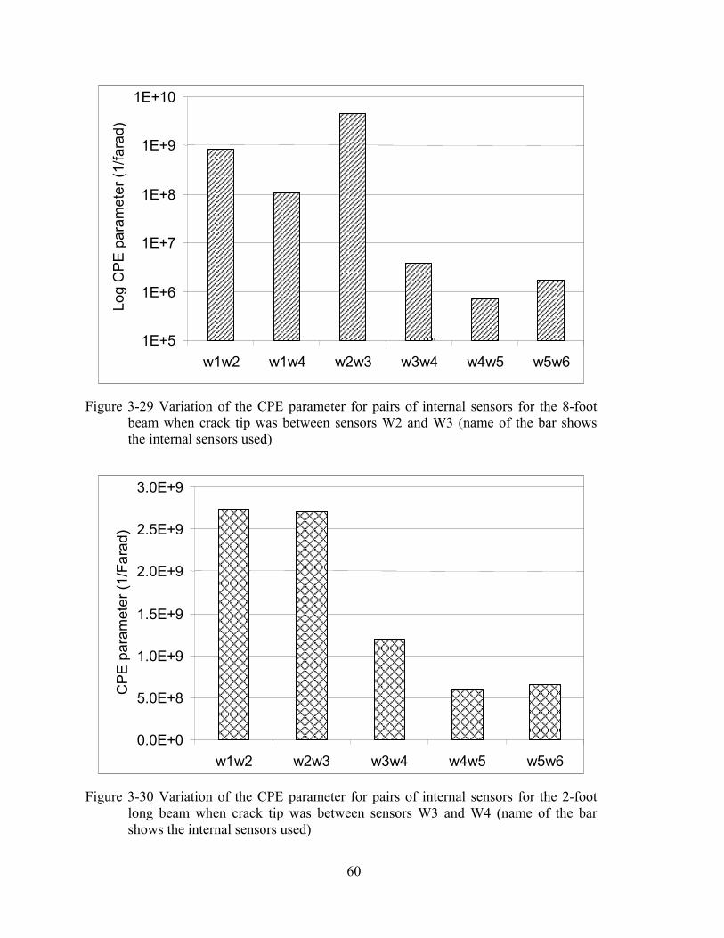
1E+5

1E+6

1E+7

1E+8

1E+9

1E+10

w1w2 w1w4 w2w3 w3w4 w4w5 w5w6

Log

CPE

par

amet

er (1

/fara

d)

Figure 3-29 Variation of the CPE parameter for pairs of internal sensors for the 8-foot beam when crack tip was between sensors W2 and W3 (name of the bar shows the internal sensors used)

0.0E+0

5.0E+8

1.0E+9

1.5E+9

2.0E+9

2.5E+9

3.0E+9

w1w2 w2w3 w3w4 w4w5 w5w6

CP

E p

aram

eter

(1/F

arad

)

Figure 3-30 Variation of the CPE parameter for pairs of internal sensors for the 2-foot long beam when crack tip was between sensors W3 and W4 (name of the bar shows the internal sensors used)

60

3.2.4 Empirical Relationships

3.2.4.1 Raw impedance spectra

Measured impedances between the rebar to an external sensor in the high-frequency

region (100,000 – 10,000 Hz) show a remarkable good fit with the empirical formula.

21 )exp( axaZ += β (3-5)

where a1, β, a2 are coefficients obtained by curve fitting x is the crack length divided by the total length of the beam

Figures 3-31 and 3-32 show curves fitted to the impedance measured at 100,000 Hz.

Table 3-1 shows the parameters for the fits for the eight-foot long beam and two-foot

long beams in the high-frequency range. Unfortunately, the parameters in Equation (3-5)

vary considerably from one fit to another and hence it is difficult to recommend values

that can be used for diagnosis purposes.

61

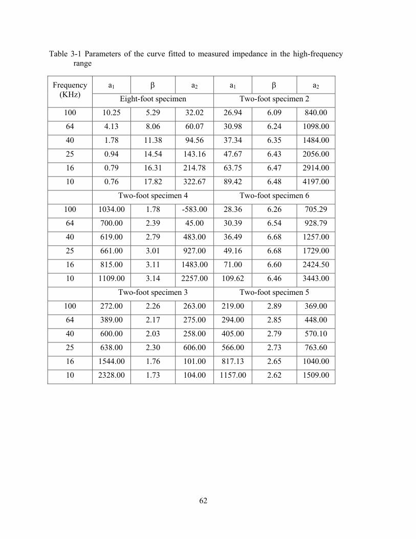
Table 3-1 Parameters of the curve fitted to measured impedance in the high-frequency range

a1 β a2 a1 β a2 Frequency (KHz) Eight-foot specimen Two-foot specimen 2

100 10.25 5.29 32.02 26.94 6.09 840.00

64 4.13 8.06 60.07 30.98 6.24 1098.00

40 1.78 11.38 94.56 37.34 6.35 1484.00

25 0.94 14.54 143.16 47.67 6.43 2056.00

16 0.79 16.31 214.78 63.75 6.47 2914.00

10 0.76 17.82 322.67 89.42 6.48 4197.00

Two-foot specimen 4 Two-foot specimen 6

100 1034.00 1.78 -583.00 28.36 6.26 705.29

64 700.00 2.39 45.00 30.39 6.54 928.79

40 619.00 2.79 483.00 36.49 6.68 1257.00

25 661.00 3.01 927.00 49.16 6.68 1729.00

16 815.00 3.11 1483.00 71.00 6.60 2424.50

10 1109.00 3.14 2257.00 109.62 6.46 3443.00

Two-foot specimen 3 Two-foot specimen 5

100 272.00 2.26 263.00 219.00 2.89 369.00

64 389.00 2.17 275.00 294.00 2.85 448.00

40 600.00 2.03 258.00 405.00 2.79 570.10

25 638.00 2.30 606.00 566.00 2.73 763.60

16 1544.00 1.76 101.00 817.13 2.65 1040.00

10 2328.00 1.73 104.00 1157.00 2.62 1509.00

62

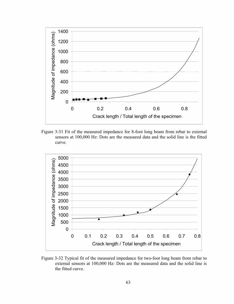
0

200

400

600

800

1000

1200

1400

0 0.2 0.4 0.6 0.8

Mag

nitu

de o

f im

peda

nce

(ohm

s)

Crack length / Total length of the specimen

Figure 3-31 Fit of the measured impedance for 8-foot long beam from rebar to external sensors at 100,000 Hz: Dots are the measured data and the solid line is the fitted curve.

0 500

1000 1500 2000 2500 3000 3500 4000 4500 5000

0 0.1 0.2 0.3 0.4 0.5 0.6 0.7 0.8

Crack length / Total length of the specimen

Mag

nitu

de o

f im

peda

nce

(ohm

s)

Figure 3-32 Typical fit of the measured impedance for two-foot long beam from rebar to external sensors at 100,000 Hz: Dots are the measured data and the solid line is the fitted curve.

63

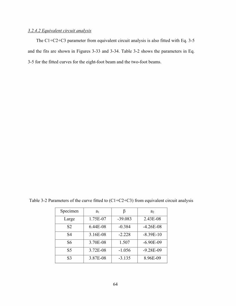
3.2.4.2 Equivalent circuit analysis

The C1+C2+C3 parameter from equivalent circuit analysis is also fitted with Eq. 3-5

and the fits are shown in Figures 3-33 and 3-34. Table 3-2 shows the parameters in Eq.

3-5 for the fitted curves for the eight-foot beam and the two-foot beams.

Table 3-2 Parameters of the curve fitted to (C1+C2+C3) from equivalent circuit analysis

Specimen a1 β a2

Large 1.75E-07 -39.083 2.43E-08

S2 6.44E-08 -0.384 -4.26E-08

S4 3.16E-08 -2.228 -8.39E-10

S6 3.70E-08 1.507 -6.90E-09

S5 3.72E-08 -1.056 -9.28E-09

S3 3.87E-08 -3.135 8.96E-09

64

0.0E+0

5.0E - 8

1.0E - 7

1.5E - 7

2.0E - 7

2.5E - 7

0.00 0.05 0.10 0.15 0.20 0.25 0.30

Crack length / Total length of the specimen

C1+

C2+

C3

para

met

er (F

arad

)

Figure 3-33 Fit for (C1+C2+C3) parameters for 8-foot beam: Dots are the measured data and the solid line is the fitted curve.

0.0E+0

5.0E-9

1.0E-8

1.5E-8

2.0E-8

2.5E-8

3.0E-8

0 0.2 0.4 0.6 0.8

C1+

C2+

C3

para

met

er (F

arad

)

Crack length / Total length of the specimen

Figure 3-34 Typical fit for (C1+C2+C3) parameters for two-foot beam: Dots are the measured data and the solid line is the fitted curve.

65

3.2.5 Summary and Discussion

The effect of CFRP debonding was studied using impedance measurements from the

rebar (R) to the copper tape sensors (Ci), and from the internal wire sensors (Wi) to the

copper tape sensors. Impedances from two-foot (medium) concrete specimens were

measured in a refrigerator and in an ambient condition at the initial crack state (4” crack

length) and at extended crack states. The large concrete beam was subjected to an

ambient condition and the crack was propagated in the ambient environment. The global

effect of interfacial cracking is best observed with the impedance measured from the

rebar to the external sensor (copper tape). The impedances measured between internal

sensors (stainless steel wires) are used to detect the location of debonded regions.

Impedance measurements at high frequencies (100,000 - 1000 Hz) yield data that have

the least sample to sample variation, and display an exponential variation with the

debonded area of CFRP.

Equivalent circuit analysis also is effective in studying CFRP debonding. The

capacitance parameters correlate best with the debonded area of CFRP. It is found that

the CPE, C1, C2+C3 and C1+C2+C3 values from equivalent circuit analysis all correlate

well with the crack length. The relationship between the C2+C3 and C1+C2+C3 values

and the debonded area of CFRP are approximately linear and show low sample-to-sample

variation. These measures have the most promise for detecting the extent of CFRP

debonding. The CPE parameter increases and the capacitance parameters decrease as the

crack is propagated.

Impedance measurements taken between pairs of internal sensors are capable of

revealing the location of regions where the CFRP is debonded from the concrete.

Measurements between pairs of sensors in debonded regions yield high impedances in the

66

low-frequency region, while those between pairs of sensors in bonded regions yield low

impedances. The CPE parameter from equivalent circuit analysis also is a strong

indicator. The CPE value corresponding to measurements between pairs of sensors in the

debonded region is about two orders of magnitude higher than that corresponding to pairs

of sensors in the bonded region. It is postulated that the reason for this distinctive

difference in the magnitude of impedance is the path of current flow in each case. When

the impedance measurement is made between sensors in the debonded area, current must

flow through the concrete, and the impedance is high. On the other hand, when

measurements are made between sensors in the bonded area, current probably flows

predominantly through the highly conductive CFRP sheet, with charge transfer between

the internal sensors and the CFRP sheet, resulting in lower impedances.

The impedance in the high-frequency range for measurements from the rebar to

external sensors and the C1+C2+C3 values are also fitted with the exponential empirical

equation in Equation (3-5). Although this equation provides an excellent fit to the data,

the parameters of the fitted equation vary widely from specimen-to-specimen and

between the two-foot and eight-foot specimens. therefore, it is difficult to recommend

parameter values that might used for diagnosis of the debonded length without first

having historical data as the debonded progresses.

67

3.3 Sensitivity of Sensor Measurements to Environmental Effects

In Section 3.2 it was demonstrated that the measured impedances in the high

frequency range and the C1+C2+C3 parameter from the equivalent circuit analysis

correlate well with debonding between the CFRP reinforcement and the concrete

substrate. In order to use these as indicators of the extent of debonding, environmental

effects on the measured impedance were studied.

3.3.1 Humidity

Experiments were performed to determine the effect of humidity on the measured

impedance over the frequency range from 0.1 Hz to 100 kHz.

3.3.1.1 Comparison of raw impedance spectra

Figures 3-35 and 3-36 show typical impedance spectra (log frequency vs log

impedance) at different humidity levels. Different humidity levels affect the magnitude of

the impedance in the low frequency region regardless of the chloride content. It should be

noted that the magnitude of impedance at a relative humidity of 60% is lower than the

magnitude of impedance at a relative humidity of 90% for the samples with chloride

(Figure 3-35). The reason for this was that the controlled environmental chamber was

malfunctioning at the time of these measurements.

Different humidity levels have a significant influence on the impedance

measurements in the low-frequency region (0.1-10 Hz). Moisture in the concrete

specimen serves as an electrolytic medium for transporting charges between sensors. At

low excitation frequencies, the current flow in the electrochemical cell (concrete

specimen) is dominated by the movement of ions (diffusion controlled), and different

68

moisture levels affects the rate of ion transport. However, it is found that different

humidity levels have less of an influence on the impedance measurements in the high-

frequency region (1000-100 kHz). The impedance is governed by the kinetics of the

charge transfer processes at the electrode-electrolyte interface at high frequencies. This

charge transfer process is influenced less by environmental conditions. The impedance

measurements from the mid-frequency range (10-1000 Hz) are somewhat sensitive to

moisture effects because at these frequencies charge transfer occurs both by diffusion and

kinetics at the interfaces.

3.3.1.2 Results from equivalent circuit analysis

The changes of moisture content in the concrete specimen influence the CPE, C1 and

C2+C3 parameters from the equivalent circuit analysis. The variation of the C1, CPE,

C2+C3 and C1+C2+C3 parameters are shown in Figures 3-37 to 3-40. Different humidity

levels have a significant influence on the CPE parameter and have less influence on the

C1 and C2+C3 parameters in the equivalent circuit analysis. Although both the C1 and

CPE parameters represent the changes of measured impedance in the low-frequency

range, it is found that the C1 parameter is less sensitive and the CPE parameter is more

sensitive to humidity variation. The value of the CPE parameter decreases with

increasing water content in the concrete specimens and the value of capacitance

parameters (C1, C2+C3, and C1+C2+C3) increase with increasing water content. The

C1+C2+C3 parameter also increases slightly as the humidity level increases.

3.3.1.3 Summary and Discussion

A change in humidity over a period of time results in a change in the water content in

the concrete specimens. Higher levels of water content lower the magnitude of

impedance, and lower levels of water content increase the magnitude of impedance in the

69

concrete specimen. Since the impedance measurements at low frequencies are governed

by the diffusion of ions which is affected by the water content, the water content in the

concrete specimen most strongly influences the measured impedance in the low-

frequency range.

70

1.0E+3

1.0E+4

1.0E+5

1.0E+6

1.0E+7

1.0E+8

1E-1 1E+0 1E+1 1E+2 1E+3 1E+4 1E+5 Log frequency (Hz)

Log

impe

danc

e (o

hms)

30% 60% 90%

Figure 3-35 Bode magnitude plot of typical impedance spectra for specimens with chloride at different humidity levels

1E+3

1E+4

1E+5

1E+6

1E+7

1E+8

1E-1 1E+0 1E+1 1E+2 1E+3 1E+4 1E+5 Log frequency (Hz)

Log

impe

danc

e (o

hms)

30% 60% 90%

Figure 3-36 Bode magnitude plot of typical impedance spectra for specimens without chloride at different humidity levels

71

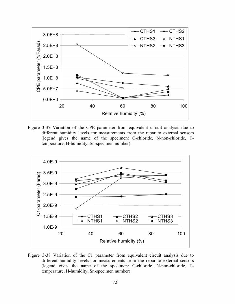
0.0E+0

5.0E+7

1.0E+8

1.5E+8

2.0E+8

2.5E+8

3.0E+8

20 40 60 80 100 Relative humidity (%)

CP

E p

aram

eter

(1/F

arad

) CTHS1 CTHS2 CTHS3 NTHS1 NTHS2 NTHS3

Figure 3-37 Variation of the CPE parameter from equivalent circuit analysis due to different humidity levels for measurements from the rebar to external sensors (legend gives the name of the specimen: C-chloride, N-non-chloride, T-temperature, H-humidity, Sn-specimen number)

1.0E-9

1.5E-9

2.0E-9

2.5E-9

3.0E-9

3.5E-9

4.0E-9

20 40 60 80 100 Relative humidity (%)

C1-

para

met

er (F

arad

)

CTHS1 CTHS2 CTHS3 NTHS1 NTHS2 NTHS3

Figure 3-38 Variation of the C1 parameter from equivalent circuit analysis due to different humidity levels for measurements from the rebar to external sensors (legend gives the name of the specimen: C-chloride, N-non-chloride, T-temperature, H-humidity, Sn-specimen number)

72

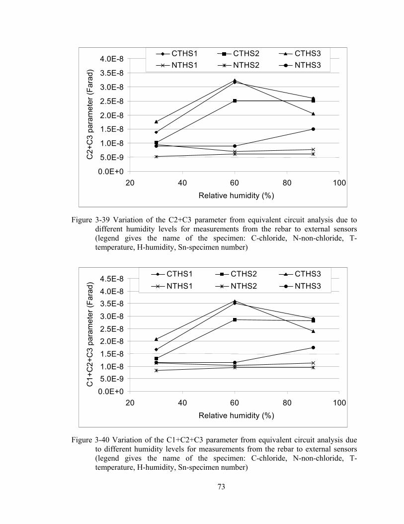
0.0E+0

5.0E-9

1.0E-8

1.5E-8

2.0E-8

2.5E-8

3.0E-8

3.5E-8

4.0E-8

20 40 60 80 100 Relative humidity (%)

C2+

C3

para

met

er (F

arad

)

CTHS1 CTHS2 CTHS3 NTHS1 NTHS2 NTHS3

Figure 3-39 Variation of the C2+C3 parameter from equivalent circuit analysis due to different humidity levels for measurements from the rebar to external sensors (legend gives the name of the specimen: C-chloride, N-non-chloride, T-temperature, H-humidity, Sn-specimen number)

0.0E+0 5.0E-9 1.0E-8 1.5E-8 2.0E-8 2.5E-8 3.0E-8 3.5E-8 4.0E-8 4.5E-8

20 40 60 80 100 Relative humidity (%)

C1+

C2+

C3

para

met

er (F

arad

)

CTHS1 CTHS2 CTHS3 NTHS1 NTHS2 NTHS3

Figure 3-40 Variation of the C1+C2+C3 parameter from equivalent circuit analysis due to different humidity levels for measurements from the rebar to external sensors (legend gives the name of the specimen: C-chloride, N-non-chloride, T-temperature, H-humidity, Sn-specimen number)

73

3.3.2 Temperature

Experiments were performed to determine the influence of temperature effects on the

measured impedance over the frequency range from 0.1 Hz to 100 kHz. Note, however,

that the humidity level was not kept constant so the moisture content in the specimens are

likely to have been different at the different temperatures.

3.3.2.1 Comparison of raw impedance spectra

Figures 3-41 and 4-42 show typical impedance spectra at different temperatures. The

slope of the impedance magnitude changes at frequencies below 1000 Hz and becomes

zero in the mid- and low-frequency region at the high temperature of 1000F. At 700F, the

slope of measured impedance becomes smaller at frequencies below 10 Hz compared to

the measured impedance at 1000F. The impedance measurements are affected in the low-

and mid-frequency regions as the temperature varies from 70 0F to 100 0F.

Measured impedances are also analyzed at specific frequencies. Figures 3-43 to 3-45

show the variation of measured impedance at different temperatures at frequencies of

10,000 Hz, 100Hz, and 1 Hz. 10,000 Hz, 100 Hz, and 1 Hz are arbitrary representative

frequencies for high-(100,000 – 1000Hz), mid- (1000 – 10 Hz), and low-frequency (10 –

0.1 Hz) ranges, respectively. The log of the magnitude at 10,000 Hz and 1 Hz show a

reasonably linear trend with increasing temperature, but the trend is more nonlinear at

100 Hz. At 100 Hz the change in temperature from 00F to 700F has a much smaller

influence of the impedance magnitude than the change in temperature from 700F to

1000F.

74

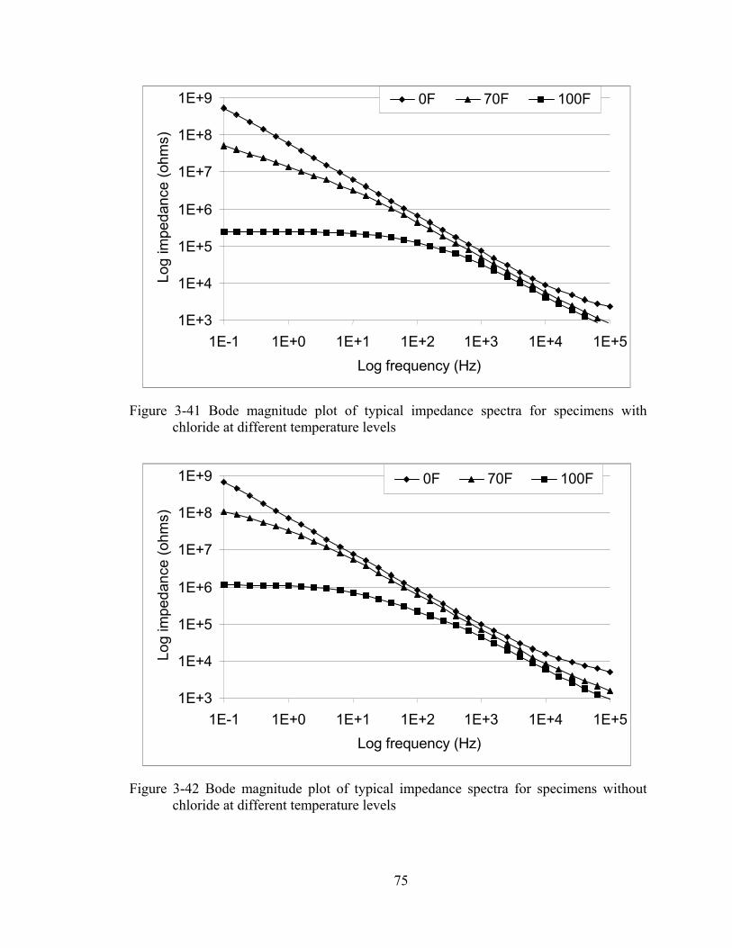
1E+3

1E+4

1E+5

1E+6

1E+7

1E+8

1E+9

1E-1 1E+0 1E+1 1E+2 1E+3 1E+4 1E+5 Log frequency (Hz)

Log

impe

danc

e (o

hms)

0F 70F 100F

Figure 3-41 Bode magnitude plot of typical impedance spectra for specimens with chloride at different temperature levels

1E+3

1E+4

1E+5

1E+6

1E+7

1E+8

1E+9

1E-1 1E+0 1E+1 1E+2 1E+3 1E+4 1E+5 Log frequency (Hz)

Log

impe

danc

e (o

hms)

0F 70F 100F

Figure 3-42 Bode magnitude plot of typical impedance spectra for specimens without chloride at different temperature levels

75

0.0E+0

2.0E+3

4.0E+3

6.0E+3

8.0E+3

1.0E+4

1.2E+4

1.4E+4

1.6E+4

1.8E+4

-10 10 30 50 70 90 110 Temperature (F)

Mag

nitu

de o

f im

peda

nce

(ohm

s) CS1 CS2 CS3

NS1 NS2 NS3

Figure 3-43 Variation of typical measured impedance in the high-frequency range at different temperature levels at 10,000 Hz (legend gives the name of the specimen: C-chloride, N-non-chloride, Sn-specimen number)

0E+0 1E+5 2E+5 3E+5 4E+5 5E+5 6E+5 7E+5 8E+5 9E+5

-10 10 30 50 70 90 110 Temperature (F)

Mag

nitu

de o

f im

peda

nce

(ohm

s) CS1 CS2 CS3

NS1 NS2 NS3

Figure 3-44 Variation of typical measured impedance in the mid-frequency range at different temperature levels at 100 Hz (legend gives the name of the specimen: C-chloride, N-non-chloride, Sn-specimen number)

76

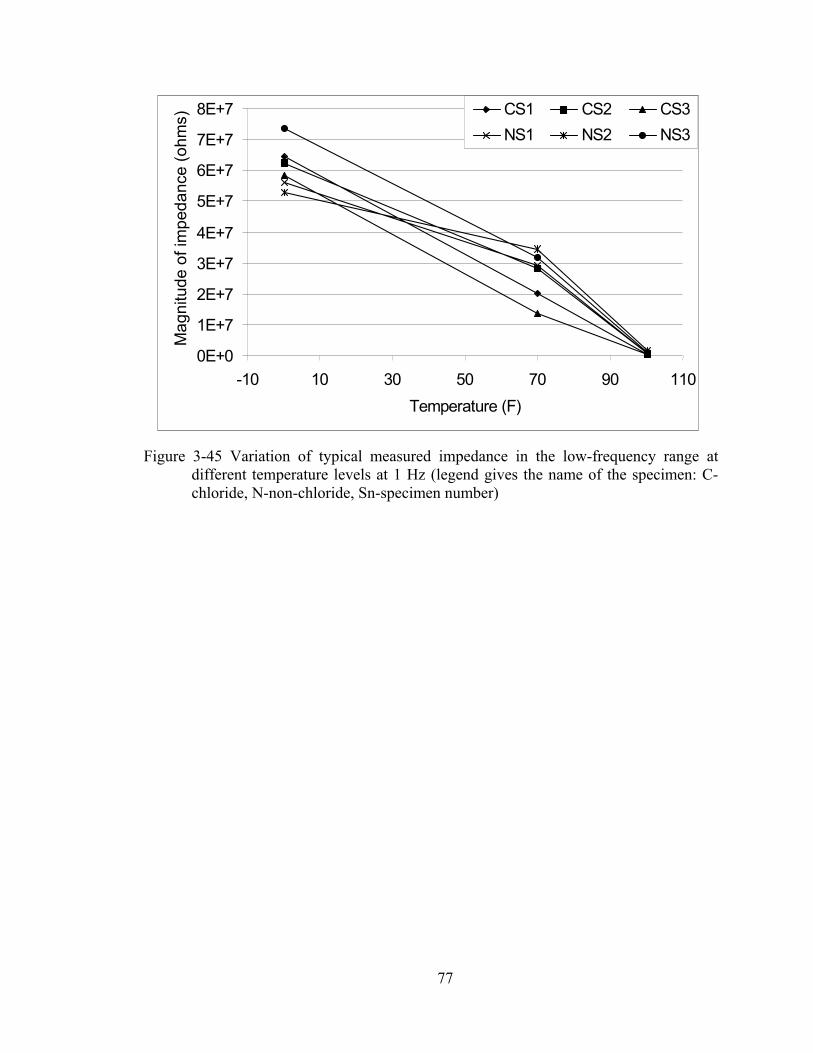
0E+0

1E+7

2E+7

3E+7

4E+7

5E+7

6E+7

7E+7

8E+7

-10 10 30 50 70 90 110 Temperature (F)

Mag

nitu

de o

f im

peda

nce

(ohm

s) CS1 CS2 CS3

NS1 NS2 NS3

Figure 3-45 Variation of typical measured impedance in the low-frequency range at different temperature levels at 1 Hz (legend gives the name of the specimen: C-chloride, N-non-chloride, Sn-specimen number)

77

3.3.2.2 Results from equivalent circuit analysis

The variation of the CPE, C1, the C2+C3 and the C1+C2+C3 parameters with

temperature are shown in Figures 3-46 to 3-49. It should be noted that the change in

temperature from 00F to 700F has a smaller influence than the change in temperature from

700F to 1000F on all the capacitance parameters. On the other hand, the change in

temperature from 00F to 700F has a larger influence on the CPE parameter than the

change in temperature from 700F to 1000F. In general, different temperatures have a

significant influence on the CPE parameter and have less influence on the C1, and the

C2+C3 and C1+C2+C3 parameters in the equivalent circuit analysis. The value of the

CPE parameter decreases with increasing temperature in the concrete specimens and the

value of capacitance parameters (C1, C2+C3) increase with increasing temperature. The

C1+C2+C3 parameter also increases slightly as the humidity level increases.

3.3.2.3 Summary and Discussion

Change in temperature in the concrete specimen has a significant influence on the

impedance measurements. At very low temperatures 00F, water in the concrete is usually

in a super-cooled state significantly slows down the diffusion of ions. This results in the

magnitude of impedance being very high. On the other hand, high temperatures increase

the mobility of ions and lower the magnitude of impedance.

78

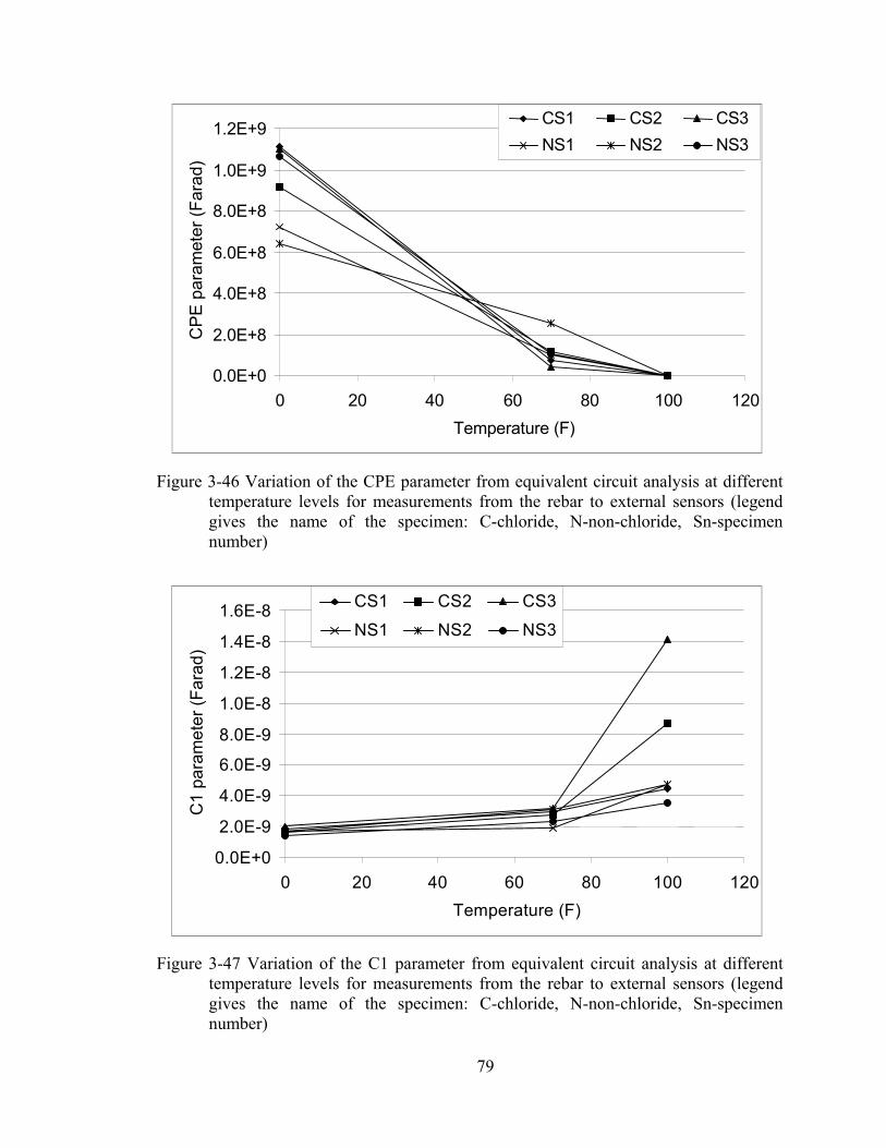
0.0E+0

2.0E+8

4.0E+8

6.0E+8

8.0E+8

1.0E+9

1.2E+9

0 20 40 60 80 100 120Temperature (F)

CP

E p

aram

eter

(Far

ad)

CS1 CS2 CS3 NS1 NS2 NS3

Figure 3-46 Variation of the CPE parameter from equivalent circuit analysis at different temperature levels for measurements from the rebar to external sensors (legend gives the name of the specimen: C-chloride, N-non-chloride, Sn-specimen number)

0.0E+0

2.0E-9

4.0E-9

6.0E-9

8.0E-9

1.0E-8

1.2E-8

1.4E-8

1.6E-8

0 20 40 60 80 100 120 Temperature (F)

C1

para

met

er (F

arad

)

CS1 CS2 CS3

NS1 NS2 NS3

Figure 3-47 Variation of the C1 parameter from equivalent circuit analysis at different temperature levels for measurements from the rebar to external sensors (legend gives the name of the specimen: C-chloride, N-non-chloride, Sn-specimen number)

79

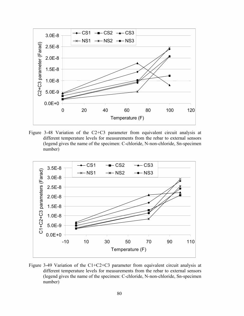
0.0E+0

5.0E-9

1.0E-8

1.5E-8

2.0E-8

2.5E-8

3.0E-8

0 20 40 60 80 100 120 Temperature (F)

C2+

C3

para

met

er (F

arad

) CS1 CS2 CS3

NS1 NS2 NS3

Figure 3-48 Variation of the C2+C3 parameter from equivalent circuit analysis at different temperature levels for measurements from the rebar to external sensors (legend gives the name of the specimen: C-chloride, N-non-chloride, Sn-specimen number)

0.0E+0

5.0E-9

1.0E-8

1.5E-8

2.0E-8

2.5E-8

3.0E-8

3.5E-8

-10 10 30 50 70 90 110 Temperature (F)

C1+

C2+

C3

para

met

ers

(Far

ad)

CS1 CS2 CS3 NS1 NS2 NS3

Figure 3-49 Variation of the C1+C2+C3 parameter from equivalent circuit analysis at different temperature levels for measurements from the rebar to external sensors (legend gives the name of the specimen: C-chloride, N-non-chloride, Sn-specimen number)

80

3.3.3 Chloride content

The experiment to study the impact of chloride content was conducted

simultaneously with the experiment to study humidity and temperature effects.

3.1.3.1 Comparison of raw impedance spectra

Figures 3-50 to 3-52 show the measured impedance spectra over the entire frequency

range at different humidity levels. Figures 3-53 to 3-55 show the impact of chloride

content at different humidity levels on the measured impedance at specific frequencies.

10,000 Hz, 100 Hz, and 1 Hz are arbitrary frequencies that represent high-(100,000 –

1000 Hz), mid- (1000 – 10 Hz), and low-frequency (10 – 0.1 Hz) ranges, respectively.

The lowering of the magnitude of impedance in the presence of chloride was observed in

the high- and low-frequency range at all three different humidity levels (30, 60 and 90%).

However, in the mid-frequency range, the presence of chloride ions has a smaller

influence on the measured impedance at the three humidity levels.

The combination of chloride content and different temperatures has less influence on

the measured impedance. Figures 3-56 to 3-58 show the measured impedance spectra

over the entire frequency range at different temperature levels. Figures 3-43 to 3-45 show

the impact of chloride content on the measured impedance at three temperatures at

specific frequencies. The presence of chloride shows a clear influence on impedance only

in the high frequency range at 00F and 700F. Nevertheless, the effect of chloride content

on the measured impedance at different temperatures is relatively minor

81

1E+3

1E+4

1E+5

1E+6

1E+7

1E+8

1E+9

1E-1 1E+0 1E+1 1E+2 1E+3 1E+4 1E+5 Log frequency (Hz)

Log

impe

danc

e (o

hms)

CS1-30% NS1-30%

Figure 3-50 Bode magnitude plot of typical impedance spectra for specimens with/without chloride at a relative humidity of 30% (legend gives the name of the specimen: C-chloride, N-non-chloride, Sn-specimen number)

1E+2

1E+3

1E+4

1E+5

1E+6

1E+7

1E+8

1E-1 1E+0 1E+1 1E+2 1E+3 1E+4 1E+5 Log frequency (Hz)

Log

impe

danc

e (o

hms)

CS1-60% NS1-60%

Figure 3-51 Bode magnitude plot of typical impedance spectra for specimens with/without chloride at a relative humidity of 60% (legend gives the name of the specimen: C-chloride, N-non-chloride, Sn-specimen number)

82

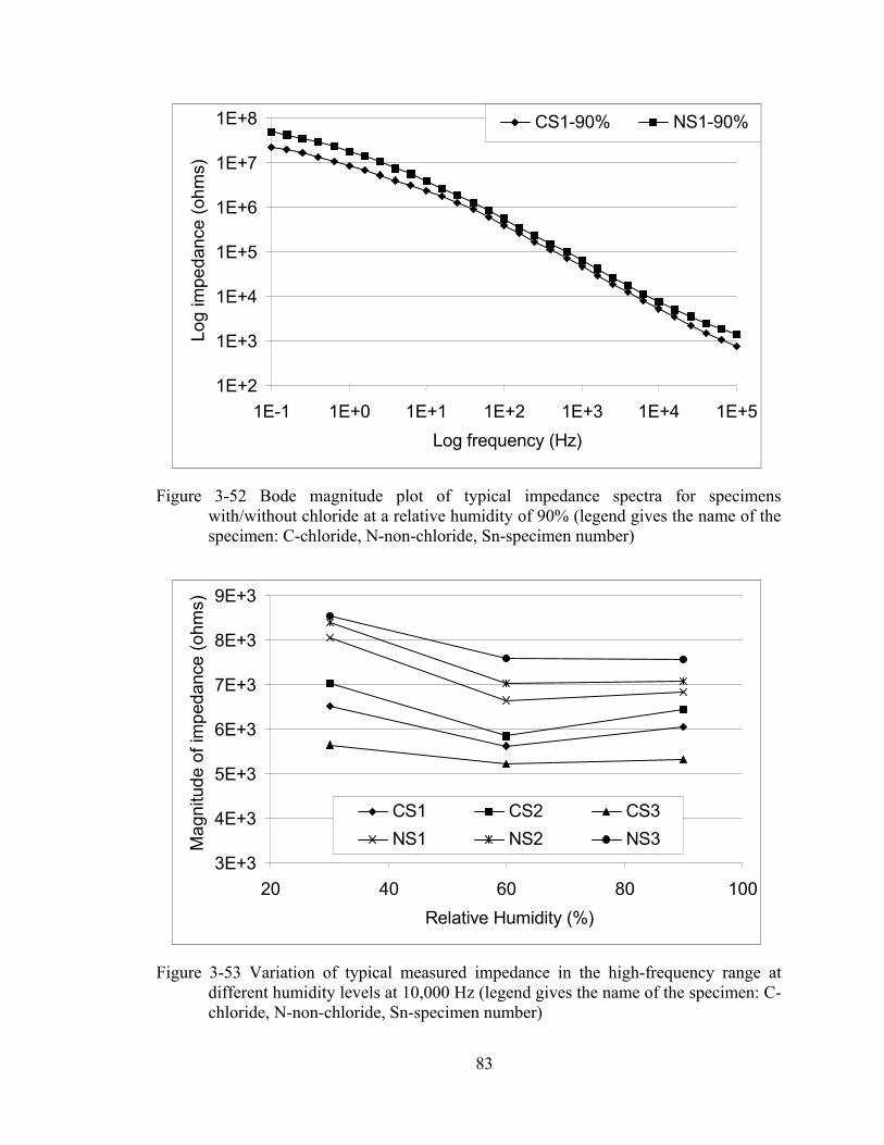
1E+2

1E+3

1E+4

1E+5

1E+6

1E+7

1E+8

1E-1 1E+0 1E+1 1E+2 1E+3 1E+4 1E+5 Log frequency (Hz)

Log

impe

danc

e (o

hms)

CS1-90% NS1-90%

Figure 3-52 Bode magnitude plot of typical impedance spectra for specimens with/without chloride at a relative humidity of 90% (legend gives the name of the specimen: C-chloride, N-non-chloride, Sn-specimen number)

3E+3

4E+3

5E+3

6E+3

7E+3

8E+3

9E+3

20 40 60 80 100 Relative Humidity (%)

Mag

nitu

de o

f im

peda

nce

(ohm

s)

CS1 CS2 CS3 NS1 NS2 NS3

Figure 3-53 Variation of typical measured impedance in the high-frequency range at different humidity levels at 10,000 Hz (legend gives the name of the specimen: C-chloride, N-non-chloride, Sn-specimen number)

83

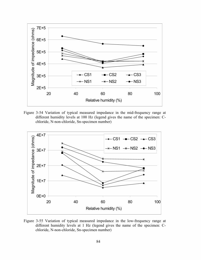
2E+5

3E+5

4E+5

5E+5

6E+5

7E+5

20 40 60 80 100 Relative humidity (%)

Mag

nitu

de o

f im

peda

nce

(ohm

s)

CS1 CS2 CS3

NS1 NS2 NS3

Figure 3-54 Variation of typical measured impedance in the mid-frequency range at different humidity levels at 100 Hz (legend gives the name of the specimen: C-chloride, N-non-chloride, Sn-specimen number)

0E+0

1E+7

2E+7

3E+7

4E+7

20 40 60 80 100 Relative humidity (%)

Mag

nitu

de o

f im

peda

nce

(ohm

s)

CS1 CS2 CS3

NS1 NS2 NS3

Figure 3-55 Variation of typical measured impedance in the low-frequency range at different humidity levels at 1 Hz (legend gives the name of the specimen: C-chloride, N-non-chloride, Sn-specimen number)

84

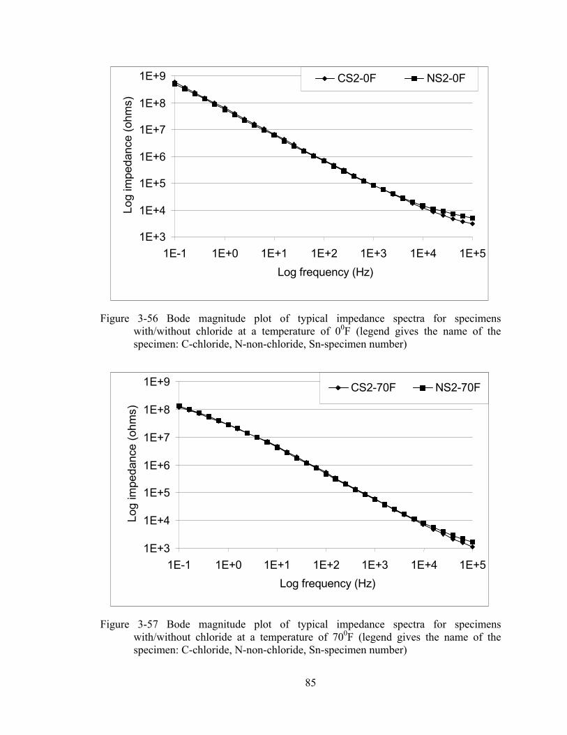
1E+3

1E+4

1E+5

1E+6

1E+7

1E+8

1E+9

1E-1 1E+0 1E+1 1E+2 1E+3 1E+4 1E+5 Log frequency (Hz)

Log

impe

danc

e (o

hms)

CS2-0F NS2-0F

Figure 3-56 Bode magnitude plot of typical impedance spectra for specimens with/without chloride at a temperature of 00F (legend gives the name of the specimen: C-chloride, N-non-chloride, Sn-specimen number)

1E+3

1E+4

1E+5

1E+6

1E+7

1E+8

1E+9

1E-1 1E+0 1E+1 1E+2 1E+3 1E+4 1E+5 Log frequency (Hz)

Log

impe

danc

e (o

hms)

CS2-70F NS2-70F

Figure 3-57 Bode magnitude plot of typical impedance spectra for specimens with/without chloride at a temperature of 700F (legend gives the name of the specimen: C-chloride, N-non-chloride, Sn-specimen number)

85

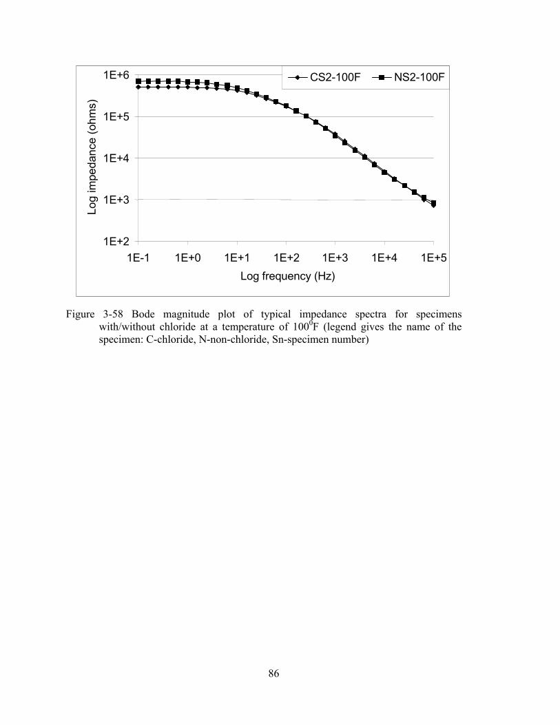
1E+2

1E+3

1E+4

1E+5

1E+6

1E-1 1E+0 1E+1 1E+2 1E+3 1E+4 1E+5 Log frequency (Hz)

Log

impe

danc

e (o

hms)

CS2-100F NS2-100F

Figure 3-58 Bode magnitude plot of typical impedance spectra for specimens with/without chloride at a temperature of 1000F (legend gives the name of the specimen: C-chloride, N-non-chloride, Sn-specimen number)

86

3.3.3.2 Results from equivalent circuit analysis

Figures 3-37 to 3-40 show the effect of chloride content on the equivalent circuit

parameters at different humidity levels. The value of the CPE parameter is decreased by

the presence of chloride ions in the concrete specimens and the value of the capacitance

parameters (C2+C3) is increased. However, there is no clear effect of the presence of

chloride ions on the C1 parameter at different humidity levels. In general, chloride

content decreases the CPE parameter and increases the C2+C3 parameter in the

equivalent circuit analysis.

Figures 3-46 to 3-49 show the variation of the equivalent circuit element parameters

due to chloride content at different temperatures. There is no discernible difference in the

equivalent circuit parameters due to the presence of chloride. The general scatter in the

parameters is within the specimen-to-specimen variation of the parameter values.

3.3.3.3 Summary and Discussion

The chloride ion content in the concrete specimen has a minor influence on the

impedance measurements. The existence of chloride ions in the concrete specimens

affects the mobility of ions. The combination of chloride ions and humidity variation has

a greater impact on the measured impedance than the combination of chloride ions and

temperature variations. In general, the presence chloride ions in the concrete specimens

lowers the magnitude of measured impedance at any humidity level and decreases the

magnitude of the impedance slightly.

87

3.3.4 Freeze – thaw

3.3.4.1 Comparison of raw impedance spectra

The magnitude of impedance before and after 300 freeze-thaw cycles is plotted in

Figure 3-59. The impedance is reduced over the entire frequency range regardless of the

water content in the concrete specimens. However, the differences are most significant in

the low- and mid-frequency ranges. The differences in the weight of the freeze-thaw

specimens before and after freeze-thaw exposure are shown in Table 3-3. The concrete

specimens were put in an oven to dry out the excessive water from the freeze-thaw

experiment. Specimens 1 and 2 contained slightly less water and Specimen 3 contained

slightly more water compared to the time when baseline measurements were taken.

3.3.4.2 Results from equivalent circuit analysis

Figures 3-60 to 3-63 show the variation of the equivalent circuit parameters

following freeze-thaw exposure. After 300 cycles of freeze-thaw the CPE parameter

dropped significantly. The C1 parameter increased, the C2+C3 parameter decreased, and

the C1+C2+C3 parameter showed little change. The variation on the capacitance

parameters from the freeze-thaw exposure is bigger than that from the short term

environmental conditions (temperature and humidity). In general, 300 cycles of freeze-

thaw have a significant influence on the CPE parameter and much smaller influences on

the C1, the C2+C3 and the C1+C2+C3 parameter obtained from the equivalent circuit

analysis.

3.3.4.3 Summary and Discussion

Freeze-thaw cycles generally tend to deteriorate the concrete and increase the width

and density of microcracks. This increases the mobility of ions within the concrete and

hence reduces the magnitude of impedance. The results indicate that the reduction in

88

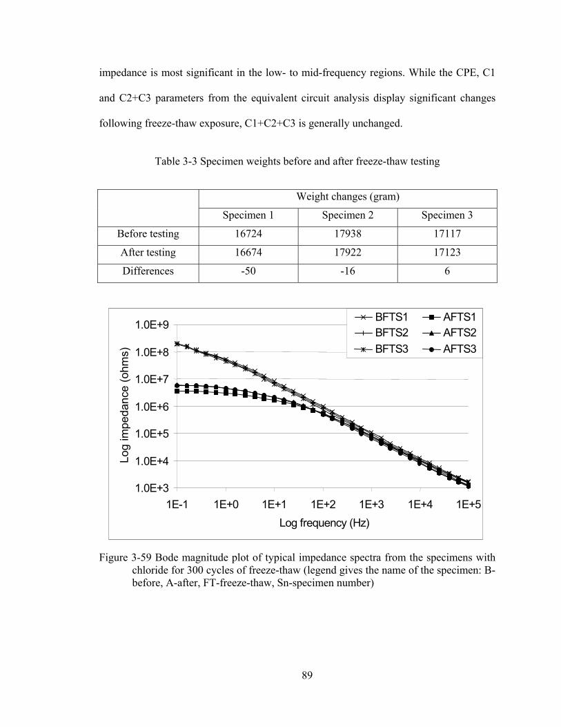
impedance is most significant in the low- to mid-frequency regions. While the CPE, C1

and C2+C3 parameters from the equivalent circuit analysis display significant changes

following freeze-thaw exposure, C1+C2+C3 is generally unchanged.

Table 3-3 Specimen weights before and after freeze-thaw testing

Weight changes (gram)

Specimen 1 Specimen 2 Specimen 3

Before testing 16724 17938 17117

After testing 16674 17922 17123

Differences -50 -16 6

1.0E+3

1.0E+4

1.0E+5

1.0E+6

1.0E+7

1.0E+8

1.0E+9

1E-1 1E+0 1E+1 1E+2 1E+3 1E+4 1E+5Log frequency (Hz)

Log

impe

danc

e (o

hms)

BFTS1 AFTS1 BFTS2 AFTS2 BFTS3 AFTS3

Figure 3-59 Bode magnitude plot of typical impedance spectra from the specimens with chloride for 300 cycles of freeze-thaw (legend gives the name of the specimen: B-before, A-after, FT-freeze-thaw, Sn-specimen number)

89

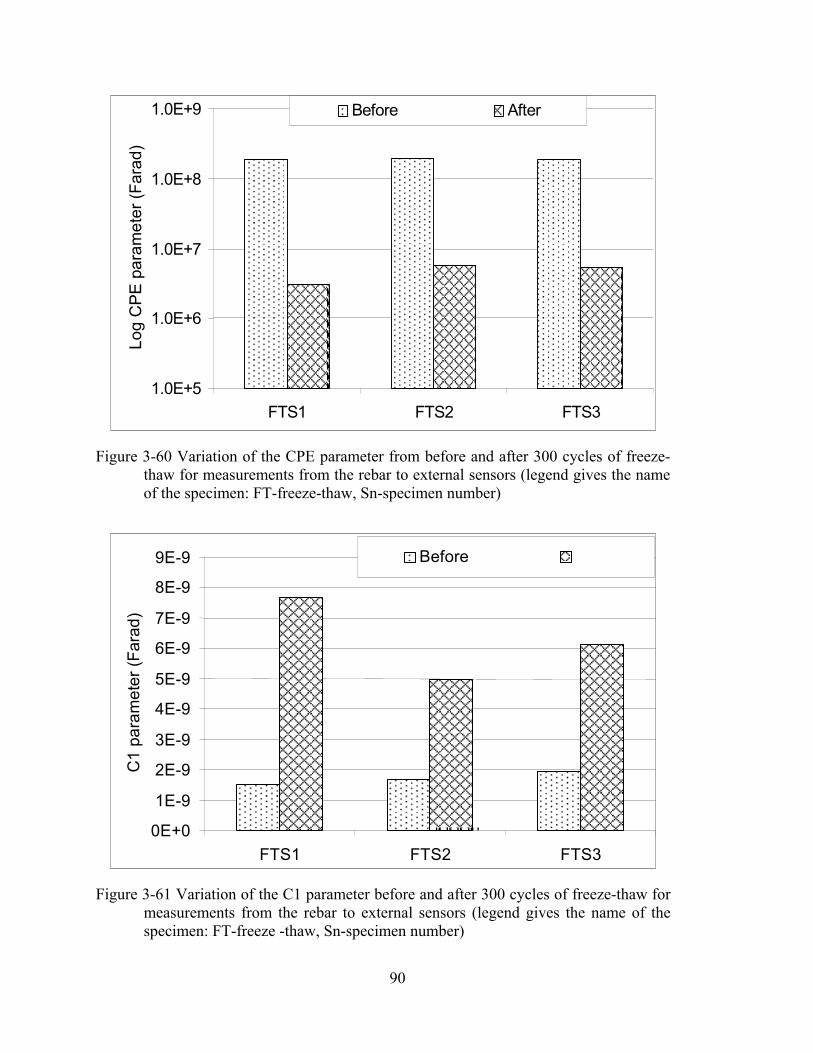
1.0E+5

1.0E+6

1.0E+7

1.0E+8

1.0E+9

FTS1 FTS2 FTS3

Log

CPE

par

amet

er (F

arad

) Before

After

After

Figure 3-60 Variation of the CPE parameter from before and after 300 cycles of freeze-thaw for measurements from the rebar to external sensors (legend gives the name of the specimen: FT-freeze-thaw, Sn-specimen number)

0E+0

1E-9

2E-9

3E-9

4E-9

5E-9

6E-9

7E-9

8E-9

9E-9

FTS1 FTS2 FTS3

C1

para

met

er (F

arad

)

Before

Figure 3-61 Variation of the C1 parameter before and after 300 cycles of freeze-thaw for measurements from the rebar to external sensors (legend gives the name of the specimen: FT-freeze -thaw, Sn-specimen number)

90

0E+0

1E-9

2E-9 3E-9

4E-9

5E-9

6E-9

7E-9 8E-9

9E-9

1E-8

FTS1 FTS2 FTS3

C2+

C3

para

met

er (F

arad

)

Before

After

After

Figure 3-62 Variation of the C2+C3 parameter before and after 300 cycles of freeze-thaw for measurements from the rebar to external sensors (legend gives the name of the specimen: FT-freeze -thaw, Sn-specimen number)

0.0E+0

2.0E-9

4.0E-9

6.0E-9

8.0E-9

1.0E-8

1.2E-8

1.4E-8

FTS1 FTS2 FTS3

C1+

C2+

C3

para

met

er (F

arad

)

Before

Figure 3-63 Variation of the C1+C2+C3 parameter before and after 300 cycles of freeze-thaw for measurements from the rebar to external sensors (legend gives the name of the specimen: FT-freeze -thaw, Sn-specimen number)

91

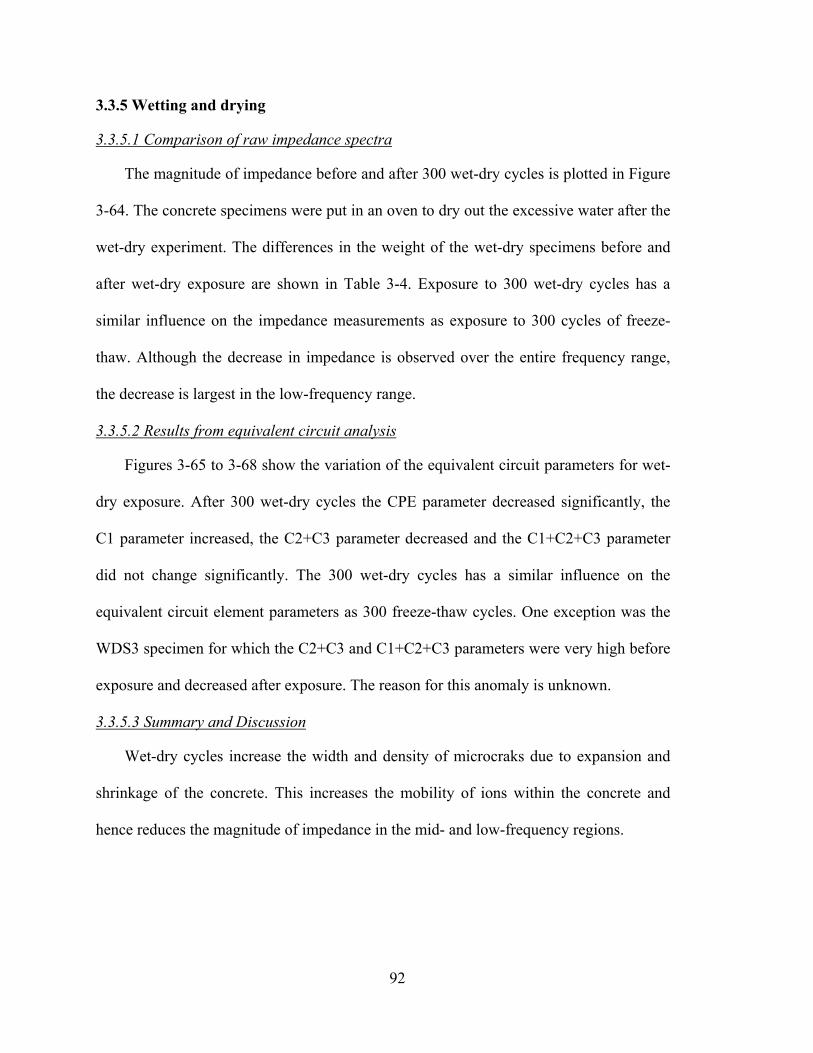
3.3.5 Wetting and drying

3.3.5.1 Comparison of raw impedance spectra

The magnitude of impedance before and after 300 wet-dry cycles is plotted in Figure

3-64. The concrete specimens were put in an oven to dry out the excessive water after the

wet-dry experiment. The differences in the weight of the wet-dry specimens before and

after wet-dry exposure are shown in Table 3-4. Exposure to 300 wet-dry cycles has a

similar influence on the impedance measurements as exposure to 300 cycles of freeze-

thaw. Although the decrease in impedance is observed over the entire frequency range,

the decrease is largest in the low-frequency range.

3.3.5.2 Results from equivalent circuit analysis

Figures 3-65 to 3-68 show the variation of the equivalent circuit parameters for wet-

dry exposure. After 300 wet-dry cycles the CPE parameter decreased significantly, the

C1 parameter increased, the C2+C3 parameter decreased and the C1+C2+C3 parameter

did not change significantly. The 300 wet-dry cycles has a similar influence on the

equivalent circuit element parameters as 300 freeze-thaw cycles. One exception was the

WDS3 specimen for which the C2+C3 and C1+C2+C3 parameters were very high before

exposure and decreased after exposure. The reason for this anomaly is unknown.

3.3.5.3 Summary and Discussion

Wet-dry cycles increase the width and density of microcraks due to expansion and

shrinkage of the concrete. This increases the mobility of ions within the concrete and

hence reduces the magnitude of impedance in the mid- and low-frequency regions.

92

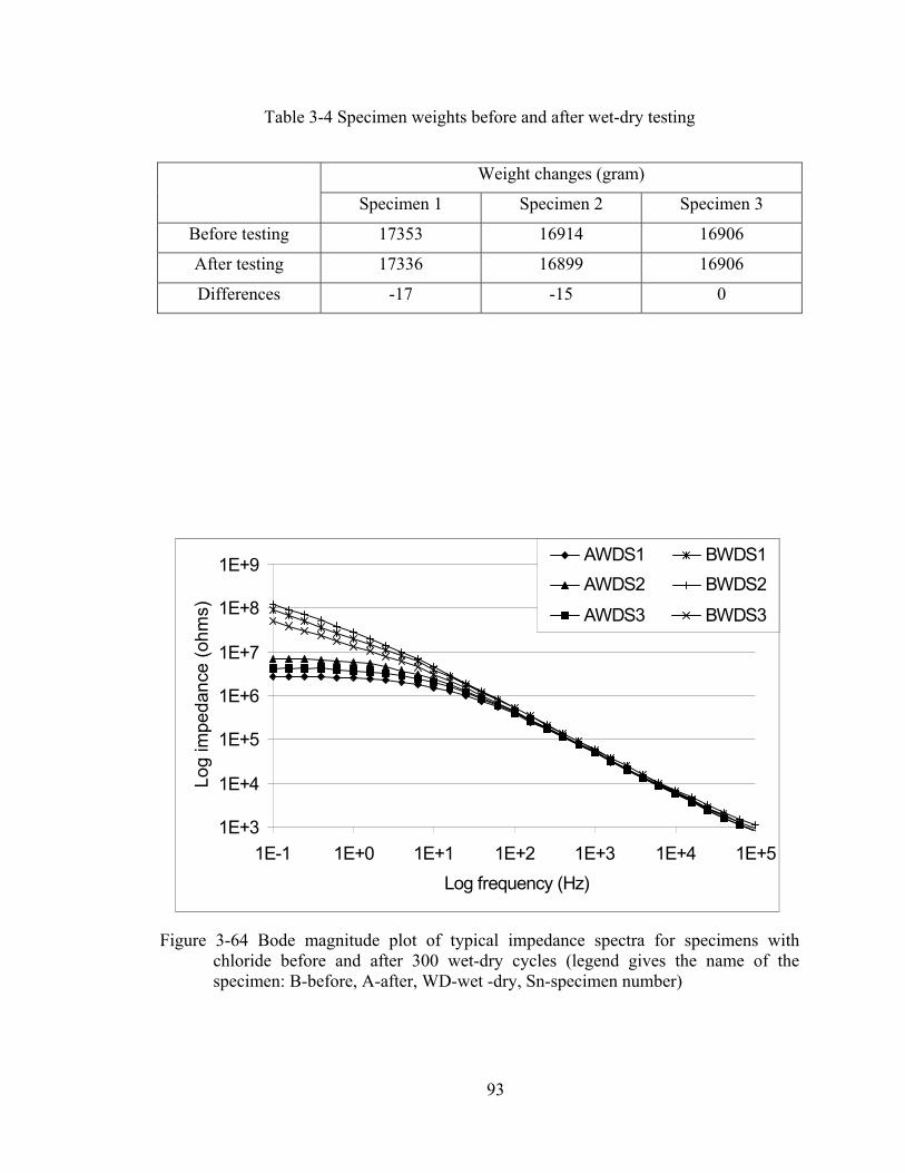
Table 3-4 Specimen weights before and after wet-dry testing

Weight changes (gram)

Specimen 1 Specimen 2 Specimen 3

Before testing 17353 16914 16906

After testing 17336 16899 16906

Differences -17 -15 0

1E+3

1E+4

1E+5

1E+6

1E+7

1E+8

1E+9

1E-1 1E+0 1E+1 1E+2 1E+3 1E+4 1E+5Log frequency (Hz)

Log

impe

danc

e (o

hms)

AWDS1 BWDS1 AWDS2 BWDS2

AWDS3 BWDS3

Figure 3-64 Bode magnitude plot of typical impedance spectra for specimens with chloride before and after 300 wet-dry cycles (legend gives the name of the specimen: B-before, A-after, WD-wet -dry, Sn-specimen number)

93

0E+0

2E+7

4E+7

6E+7

8E+7

1E+8

1E+8

WDS1 WDS2 WDS3

CP

E p

aram

eter

(1/F

arad

) Before

After

After

Figure 3-65 Variation of the CPE parameter from before and after 300 cycles of wet-dry for measurements from the rebar to external sensors (legend gives the name of the specimen: WD-wet -dry, Sn-specimen number)

0E+0

1E-9

2E-9

3E-9

4E-9

5E-9

6E-9

7E-9

WDS1 WDS2 WDS3

C1

para

met

er (F

arad

)

Before

Figure 3-66 Variation of the C1 parameter before and after 300 cycles of wet-dry for measurements from the rebar to external sensors (legend gives the name of the specimen: WD-wet -dry, Sn-specimen number)

94

0.0E+0

5.0E-9

1.0E-8

1.5E-8

2.0E-8

2.5E-8

3.0E-8

3.5E-8

4.0E-8

4.5E-8

WDS1 WDS2 WDS3

C2+

C3

para

met

ers

(Far

ad)

Before

After

After

Figure 3-67 Variation of the C2+C3 parameter before and after 300 cycles of wet-dry for measurements from the rebar to external sensors (legend gives the name of the specimen: WD-wet -dry, Sn-specimen number)

0E+0

1E-8

2E-8

3E-8

4E-8

5E-8

WDS1 WDS2 WDS3

C1+

C2+

C3

para

met

ers

(Far

ad)

Before

Figure 3-68 Variation of the C1+C2+C3 parameter before and after 300 cycles of wet-dry for measurements from the rebar to external sensors (legend gives the name of the specimen: WD-wet -dry, Sn-specimen number)

95

3.3.6 Corrosion of reinforcing bar

A constant voltage of 12 V was supplied across the two reinforcing bars to accelerate

the corrosion process using an external power source. The applied current was monitored

during 21 days of the accelerated corrosion test, since this has a direct correlation with

the total corrosion in the reinforcing bar. Steel loss was calculated using the recorded

current using (Philips 1992, Pantazopoulou 2001).

FzAmtIgW

***)( =∆ (3-1)

where ∆W is the steel loss in grams I is the total recorded current t is the duration of the test in seconds Am is the atomic mass of the metal z is valency (assuming that the rust product is mainly

Fe(OH)2, 2 is used for the z value) F is Faraday’s constant

The total steel loss was about 13g for each specimen. This represents an average

corrosion depth of about 0.45mm (3.6% loss) over the bar

3.3.6.1 Comparison of raw impedance spectra

Exposure to accelerated corrosion of the reinforcing bar has a similar influence on

the impedance measurements as exposure to freeze-thaw and wet-dry cycles. The

magnitude of measured impedances before and after accelerated corrosion are plotted in

Figures 3-69. The impedance in the low- and mid-frequency range decreased. The

differences in the weight of the specimens before and after the corrosion test are shown in

Table 3-5. Some of the mass loss is probably due to the diffusion of corrosion products

into the water used to periodically wet the specimens. The concrete specimens were put

in an oven to dry out the excessive water from the corrosion experiment.

96

3.3.6.2 Results from equivalent circuit analysis

Figures 3-70 to 3-73 show the changes in the equivalent circuit parameters after the

accelerated corrosion test. The CPE parameter decreased significantly after accelerated

corrosion for 21 days. The capacitance parameters do not change significantly due to

corrosion of the reinforcing bar in the concrete specimens. The C1 parameter increased

slightly, and the C2+C3 and C1+C2+C3 quantities did not change significantly.

3.3.6.3 Summary and Discussion

The electrical properties of the reinforcing bar and surrounding concrete may change

due to corrosion of the reinforcing bar and the presence of corrosion products in the

concrete. The corrosion test was setup to study the effect of corrosion of the reinforcing

bar on the impedance measurements. It is found that the corrosion of the reinforcing bar

significantly lowers the impedance in the low-frequency range, but has a much smaller

influence on the measured impedance in the mid- and high-frequency ranges. As a

consequences, corrosion of the reinforcing bar has a significant influence on the CPE

parameter from the equivalent circuit analysis, and has a much smaller influence on the

capacitance parameters.

97

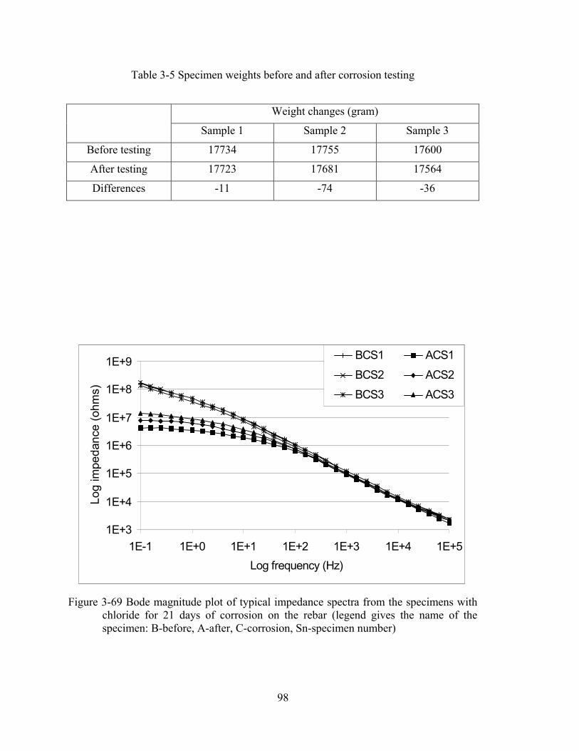
Table 3-5 Specimen weights before and after corrosion testing

Weight changes (gram)

Sample 1 Sample 2 Sample 3

Before testing 17734 17755 17600

After testing 17723 17681 17564

Differences -11 -74 -36

1E+3

1E+4

1E+5

1E+6

1E+7

1E+8

1E+9

1E-1 1E+0 1E+1 1E+2 1E+3 1E+4 1E+5 Log frequency (Hz)

Log

impe

danc

e (o

hms)

BCS1 ACS1

BCS2 ACS2

BCS3 ACS3

Figure 3-69 Bode magnitude plot of typical impedance spectra from the specimens with chloride for 21 days of corrosion on the rebar (legend gives the name of the specimen: B-before, A-after, C-corrosion, Sn-specimen number)

98

0.0E+0

2.0E+7

4.0E+7

6.0E+7

8.0E+7

1.0E+8

1.2E+8

1.4E+8

1.6E+8

1.8E+8

CCS1 CCS2 CCS3

CP

E p

aram

eter

(Far

ad)

Before

After

After

Figure 3-70 Variation of the CPE parameter from equivalent circuit analysis for specimens with chloride before and after 21 days of rebar corrosion for measurements from the rebar to external sensors (legend gives the name of the specimen: C-chloride, C-corrosion, Sn-specimen number)

0.0E+0

5.0E-10

1.0E-9

1.5E-9

2.0E-9

2.5E-9

3.0E-9

3.5E-9

4.0E-9

CCS1 CCS2 CCS3

C1

para

met

er (F

arad

)

Before

Figure 3-71 Variation of the C1 parameter from equivalent circuit analysis for specimens with chloride before and after 21 days of rebar corrosion for measurements from the rebar to external sensors (legend gives the name of the specimen: C-chloride, C-corrosion, Sn–specimen number)

99

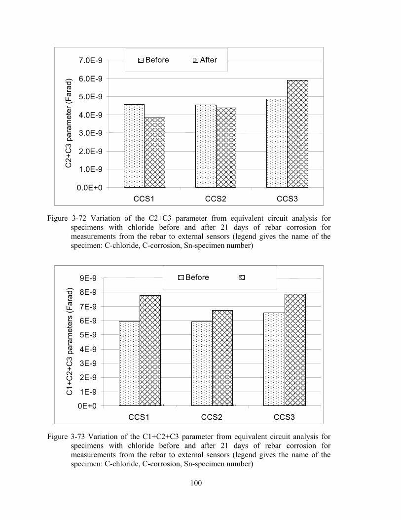
0.0E+0

1.0E-9

2.0E-9

3.0E-9

4.0E-9

5.0E-9

6.0E-9

7.0E-9

CCS1 CCS2 CCS3

C2+

C3

para

met

er (F

arad

) Before

After

After

Figure 3-72 Variation of the C2+C3 parameter from equivalent circuit analysis for specimens with chloride before and after 21 days of rebar corrosion for measurements from the rebar to external sensors (legend gives the name of the specimen: C-chloride, C-corrosion, Sn-specimen number)

0E+0

1E-9

2E-9

3E-9

4E-9

5E-9

6E-9

7E-9

8E-9

9E-9

CCS1 CCS2 CCS3

C1+

C2+

C3

para

met

ers

(Far

ad)

Before

Figure 3-73 Variation of the C1+C2+C3 parameter from equivalent circuit analysis for specimens with chloride before and after 21 days of rebar corrosion for measurements from the rebar to external sensors (legend gives the name of the specimen: C-chloride, C-corrosion, Sn-specimen number)

100

3.4 Effect of electrode size

Figure 3-74 shows the measured impedance from the CFRP sheet (external sensor)

to the different sized electrodes in the 6” x 2’ x 1’ slab constructed to study the effect of

the electrode size. The different electrode sizes affect only the measured impedance in the

very high frequency region (10,000 - 1000,000 Hz) which are controlled by the kinetics

of the charge transfer processes at the electrode/electrolyte interfaces. A larger effective

electrode area increases the kinetic potential energy. As a result, the measured impedance

decreases in the high frequency range. It should be noted that the measured impedance

from the E3, E4 and E5 sensors to the external sensor yield very similar values over the

entire frequency range. This suggests that increasing the electrode size beyond a certain

limit does not have a significant impact on the measured impedance. This is also reflected

in the measured impedance from the stainless steel bar and the reinforcement cage to the

external sensor for the eight-foot long beam (Figure 3-21). The measured impedance

from the stainless steel bar and the reinforcement cage were very similar to each other

even in the high frequency region.

101

1E+2

1E+3

1E+4

1E+5

1E+6

1E+7

1E-1 1E+0 1E+1 1E+2 1E+3 1E+4 1E+5 Log frequency (Hz)

Log

impe

danc

e (o

hms)

E1 E2 E3 E4 E5

Figure 3-74 Bode magnitude plot of impedance spectra from the slab with different sized sensors (legend gives the name of the sensor: E1-0.034” dia., E2-0.25” dia., E3-0.5” dia., E4-0.59” dia., E5-0.75” dia.)

102

Chapter 4

Summary, Conclusions, and Recommendations for Future Work

4.1 Summary

An experimental study was conducted to assess whether electrochemical impedance

spectroscopy (EIS) could be used to detect the debonding of external CFRP

reinforcement on concrete structures. The EIS-based sensing technology used in this

study was adopted from work done by Davis et al. (1999) on composite/composite bonds.

Wedge tests were conducted with several 6” x 6” x 24” specimens and one 1.5’ x 2’

x 8’ specimen to investigate the detection of CFRP debonding. Sensor elements

(electrodes) consisted of: (a) copper tape with a conductive adhesive applied to the

outside of the CFRP; (b) stainless steel wire placed in grooves on the bottom face of the

concrete prior to bonding the CFRP; and (c) reinforcing bars. Experimental studies were

conducted to also determine the influence of different environmental conditions on

impedance measurements. The environmental conditions included: (1) variation of

humidity levels; (2) variation of temperature levels; (3) chloride content in the concrete

specimen; (4) 300 freeze-thaw cycles; (5) 300 wet-dry cycles; and (6) 21 days of

accelerated corrosion of a reinforcing bar.

Impedance measurements were taken between pairs of sensors using a potentiostat.

The measurements were analyzed by comparing the raw impedance spectra and using

equivalent circuit analysis. The raw impedance measurements for different environmental

conditions and different debonded lengths were compared either over the entire

103

frequency range or at specific frequencies. An equivalent circuit was conceived and fitted

to each measured impedance spectrum and the circuit parameters were estimated. The

fitted circuit parameters were compared for measurements from different environmental

conditions and to different CFRP debond lengths. The raw impedance measurements and

the fitted capacitance parameters (C1+C2+C3) for different debonded lengths are also

fitted to the empirical formula (Equation 3-5)

4.1.1 Detection of CFRP Debonding

Variations in the measured impedance spectra and the equivalent circuit parameters

due to debonding of the CFRP sheet was studied in a controlled environment (controlled

temperature and humidity) and in an ambient condition (fluctuating temperature and

humidity). Impedance measurements taken between the rebar and the extended copper

tape sensors were most effective for assessment of the total debonded area. Impedance

measurements taken between pairs of internal wire sensors were capable of revealing the

location of debonded regions.

CFRP debonding increased the measured impedances over the entire frequency

range when the wedge test was conducted in the controlled environment. However, when

the wedge test was conducted in the ambient condition, the measured impedances from

the low- and mid-frequency range were influenced by the different temperature and

humidity levels. The CFRP debonding effect was most clearly observed with the

impedance at high-frequencies regardless of the environmental condition. The measured

impedance at a given high frequency increases exponentially as the debond length

increases. It is found that different effective electrode areas (size effect) has a significant

influence on the measured impedance. A larger effective electrode area decreases the

magnitude of measured impedance significantly. The debonding of the CFRP was

104

capable of being detected without interference from environmental conditions by

impedances measured in the very high-frequency range from about 10,000 to 100,000

Hz. For the large specimen, even the high frequency impedances were influenced by the

environmental conditions. The increase effective electrode areas for the lorge beam

reduced the impedance magnitudes, and it is postulated that this made the measurements

more sensitive to environmental effects.

The CPE parameter in the equivalent circuit correlated well with debonded area in

the controlled environment but was strongly influenced by variations in temperature and

humidity. Capacitance parameters also correlated well with the debonded area and were

not too sensitive to environmental factors. All capacitance parameters showed a linear

correlation with the debonded area for the wedge test on two-foot long specimens. The

sum of all capacitances (C1+C2+C3) showed the least sample-to-sample variation. For

the wedge test on the large beam the sum of the capacitances (C1+C2+C3) showed an

exponentially decaying variation with debonded area with high sensitivity for initial

debonding up to about 10% of the total CFRP area.

The raw impedance measurements from the high frequency region and the fitted

capacitance parameters (C1+C2+C3) for different debonded lengths were fitted to an

empirical formula. Although the fit were always excellent, the parameters of the

empirical formula vary significantly from sample to sample and therefore a formula for

diagnosis cannot be readily proposed.

105

4.1.2 Environmental effects

The influence of short-term environmental effects including different humidity

levels, different temperature levels and chloride content in the concrete on the impedance

measurements were studied using small specimens. These environmental factors have a

significant influence on the magnitude of impedance measured in the low- and mid-

frequency range, but have a much smaller influence on the magnitude of impedance in

the high-frequency range. Increased water content due to high humidity lowered the

magnitude of impedance, and reduced water content due to low humidity increased the

magnitude of impedance. High temperature decreased the magnitude of impedance

significantly in the low- and mid-frequency range. The presence of chloride ions in

concrete increased the impedance measurements in the low- and mid-frequency range.

The influence of long-term environmental conditions including freeze-thaw and wet-

dry cycles and corrosion of the reinforcing bar on the measured impedance were also

studied. Impedance measurements were taken before and after small concrete specimens

were subjected to 300 freeze-thaw and wet-dry cycles. Impedance measurements were

also taken before and after one reinforcing bar in each small specimen was subjected to

accelerated corrosion to study the effect of corrosion on the measured impedance,

especially when the rebar was used as a sensing element. These long-term environmental

conditions had a significant influence on the measured impedance in the low-frequency

range and had much less of an influence in the high-frequency range. The magnitude of

impedance in the low-frequency range was reduced after the environmental exposure.

In the equivalent circuit, the R1, C1 and CPE parameters control the impedance in

the low-frequency region and the C2, C3, R2 and R3 parameters control the impedance in

the mid- and high-frequency regions. The different environment conditions had a

106

significant influence on the CPE parameter and had much less of an influence on the

capacitance parameters from the equivalent circuit analysis. High temperature and high

moisture content in concrete decreased the CPE parameter and increase the capacitance

parameters. Low temperature and low moisture content in concrete had the opposite

effects. Chloride content in concrete decreased the CPE parameter and increased the

capacitance parameters. Freeze-thaw cycles, wet-dry cycles and corrosion of the rebar

increased the CPE and C1 parameters and decreased the C2+C3 values. The sum of all

capacitance parameters (C1+C2+C3) showed the least variation after exposure to the

long-term environmental conditions.

4.2 Conclusions

Impedance measurements taken between steel reinforcement and copper tape sensors

mounted on the outside of external CFRP reinforcement are effective for estimating the

total debonded area of CFRP. Measurements taken in the high-frequency range (1000 –

100,000 Hz) are the most reliable since they are not strongly influenced by environmental

conditions. A more reliable approach is to perform equivalent circuit analysis using the

circuit used in this work, and use the sum of the capacitance parameter (C1+C2+C3) as a

measure of the total debonded area of CFRP. The impedance magnitude at a given high

frequency (say 100,000 Hz), and C1+C2+C3 values correlate well with the debonded

area of CFRP and are not strongly affected by environmental conditions. The impedance

at high frequencies is dominated by the kinetics of the charge transfer processes at the

electrode/electrolyte interfaces, which appear to be influenced strongly by the debonding

of the CFRP.

107

Impedance measurements taken between pairs of internal stainless steel wire sensors

placed in grooves cut into the bottom face of concrete beams before the CFRP is bonded

are effective in locating debonded regions. The magnitude of impedances at low

frequencies taken between a pair of sensors in the debonded region are much higher than

those taken between a pair of sensors in the bonded region. The CPE parameter from the

equivalent circuit analysis is the most effective measure for detecting the location of

debonded regions. The CPE parameter value corresponding to impedance measurements

between sensors in the debonded area is about two orders of magnitude larger than the

value corresponding to impedance measurements between sensors in the bonded area.

Short-term environmental conditions including humidity, temperature, and chloride

content affect the impedance measurements at low frequencies. The short-term

environmental conditions affect the rate of ions diffusion through the concrete, which is

the dominant mechanism for charge transfer at low frequencies. Increased moisture

content, and temperature, and the presence of chloride, increase the charge transfer rate

and hence reduce the impedance at low frequencies.

Long-term environmental conditions including freeze-thaw and wet-dry cycles, and

corrosion of the steel reinforcement, also affect the impedance measurements at low- and

mid-frequencies. The long-term environmental conditions promote the growth of micro

and macro cracks within the concrete. Repeated expansion and shrinkage due to freeze-

thaw and wet-dry cycles increase micro cracking. The expansion of volume associated

with corrosion of the rebar causes cracking of the concrete. The increase in voids

increases the diffusion rate of ions and thereby reduces the magnitude of impedance at

low frequencies.

108

4.3 Recommendations for Future Work

The EIS-based sensor technology shows strong promise for effective NDE of

concrete structures strengthened with CFRP sheets. However, results from this purely

experimental research indicate that the EIS-based impedance measurements are

influenced significantly by environmental conditions and different effective electrode

areas especially in the low- and mid-frequency range. It is also observed that the

measured impedance can have significant sample-to-sample variation.

A significant contribution to the further enhancement of this work would be the

development of a numerical approach for modeling the charge transfer process through

the specimen. This can be most effectively done at the macro-scale by using a 3-D finite

element model to represent the concrete structure, reinforcement and sensors and

effective electrical properties to represent the current condition through the various

component. The effective electrical properties of concrete would need to be characterized

with respect to temperature, humidity, chloride content, and microcrack width and

density. Once such a model is developed it can be used to study different structureal

components reinforced with CFRP, develop optimal sensor arrangements, and develop

nomographs that can be used for diagnosis of CFRP debonding.

109

110

REFERENCES

Bard, A.J., and Faulkner, L.R. (1980). Electrochemical methods: fundamentals and application. Interscience Publication, New York.

Buyukozturk, O., and Hearing, B. (1998). “Failure behavior of precracked concrete beams retrofitting with FRP.” Journal of composites for construction: 138-144.

Dai, S.T., and Labuz, J.F. (1998). “Damage and failure analysis of brittle materials by acoustic emission” Journal of Materials in Civil Engineering, Vol. 9 (4).

Davis, G.D., Dacres, C.M. and Krebs, L.A. (1999). “In-Situ sensor to detect moisture intrusion and degradation of coatings, composites, and adhesive bonds.” Proc. Tri-Services conference on corrosion, Myrtle Beach, South Carolina.

Davis, G.D., Krebs, L.A., Drzal, L.T., Rich, M.J., and Askeland, P. (2000). “Electro-chemical sensors for nondestructive evaluation of adhesive bonds.” J. Adhes. 72:335-358.

Gamry Instruments, (1999). Gamry framework system User’s manual revision 3.1.

Gamry Instruments, (April 2003) “Application notes: Equivalent circuit modeling using the Gamry EIS300 electrochemical impedance spectroscopy software.” Gamry Instruments, July 2003. <http://www.gamry.com/G2/Appnotes/Reference/ EISModeling/EISModeling.htm>

Karbhari, V.M., and Zhao, L. (2000). “Use of composites for 21st century civil infrastructure.” Computer Method in Applied Mechanics and Engineering 185: 433-454.

Macdonald, J.R. (1987). Impedance spectroscopy: emphasizing solid materials and systems : Wiley-Interscience Publication, New York.

Mirmiran, A., Shahawy, M., and Echary, J. (1999). “Acoustic emission monitoring of hybrid FRP-concrete columns.” Journal of Engineering Mechanics, Vol 125 (8).

Mirmiran, A., and Yunmei, W. (2001) “Damage assessment of FRP-encased concrete using ultrasonic pulse velocity.” Journal of Engineering Mechanics, Vol 127 (2): 126-135.

Nguyen, D.M., Chan, T.K., and Cheong, H.K. (2001). “Brittle failure and bond development length of CFRP-concrete beams.” Journal of Composites for Construction. February: 12-17.

Olajide, D., Laurence, J., and Rami M. (2000). “Ultrasonic monitoring of material degradation in FRP composites.” Journal of Engineering Mechanics Vol. 126 (7): 704-710.

111

Pantazopoulou, S., Bonacci, J, Sheikh, S., Hearn, N., and Thomas, M. (2001). “Repair of corrosion-damaged columns with FRP wraps.” Journal of composites for construction. Vol. 5 (1): 3-11.

Philips, J. (1992). “The effect of corrosion on the structural performance of new and repaired one-way slabs.” PhD thesis, Dept. of Civ. Engineering, University of Toronto.

Rahimi, H., and Hutchinson, A. (2001). “Concrete beams strengthened with externally bonded FRP plates.” Journal of Composites for Construction. February : 44-56.

Scully, J., and Kendig, M. (1989). “Basic aspects of the application of electrochemical impedance for the life prediction of organic coatings on metals.” Proc. Corrosion 89 Paper 32, NACE.

112

Appendix A

Data Collection and Equivalent Circuit Analysis Procedure

This section provides a step-by-step description of the procedures used to measure

impedances and perform equivalent circuit analysis. Additional information is provided

in the User’s Manual for the Gamry Framework software.

A-1 Software Procedure for Data Collection

The procedure described below is based on the Gamry Framework software version

3.20.

1. Connect the blue, green and white cables on the potentiostat to one sensor and the

red and orange cables to the second sensor.

2. Run the Gamry Framework software.

3. From the Gamry Framework menu bar, select Experiment, click on A

Electrochemical Impedance, and click on Potentiostatic EIS to launch the

Potentiostatic EIS window.

4. Necessary information can be filled out on the Potentiostatic EIS window or

retrieved from a saved template setup file.

5. To use a the saved template setup file, click on the Restore button located at the

top of the Potentiostatic EIS window, to display the Restore Setup window.

6. From the Restore Setup window, select a proper template setup file and select a

stored setup (each template setup file can contain several different setting), and

then click on the Restore button (this brings back to the Potentiostatic window).

7. Specify the output file name and click the OK button.

113

A-2 Equivalent circuit analysis procedure

The procedure described below is based on The Gamry Echem Analyst application

version 1.02.

1. Run the Gamry Echem Analyst application

2. Open the measured EIS data file by clicking File on the menu bar, clicking Open

File, then selecting the EIS file.

3. Click Impedance on the menu bar and then click Fit A Model. This brings up the

Select Model File window. Since the parameters of an electrical circuit which has an

theoretical impedance similar to that of the measured impedance are estimated,

selecting a proper equivalent circuit is very important.

4. Once the proper equivalent circuit model is selected, the Impedance Fitting window

is displayed. The nonlinear least squares fitting procedure requires initial values to be

specified. The initial values for each equivalent circuit are stored with the circuit. To

check whether the initial values are reasonable for the measured data, click Preview

in the Impedance Fitting window.

4.1. If the impedance generated by the equivalent circuit does not match the measured

impedance, then the initial value should be changed to obtaina better match. The

initial values for the equivalent circuit element parameters used in this research

are listed in Table A-1. Figure A-1 shows the fitted impedance using poor initial

values.

4.2. The C1, R1 and CPE parameters controls the fitted impedance in the low-

frequency range and the C2, R2, C3 and R3 parameters controls the fitted

impedance in the mid- and high-frequency ranges. Use the Preview function and

114

adjust the initial value of the parameters. If the initial values are within a factor

of 100 and the shapes of the impedance spectra generated by the initial values are

similar to the measured spectra then the equivalent circuit model will usually

yield a good fit.

4.3. Once reasonable initial values are obtained, the fitting program will converge on

parameters that yield a theoretical impedance close to the measured impedance.

Figure A-2 shows the fitted impedance with the initial values of the parameters

and the fitted impedance from the final converged values of the parameters. The

fitting program uses a Levenberg-Marquardt non-linear least square fitting

algorithm.

5. To finalize the fitting process, click the Calculate button in the Impedance Fitting

window.

Table A- 1. Initial values of equivalent circuit element parameters

Rebar to External Internal to Internal Internal to External Parameter

Low High Low High Low High

R1 1.0E+03 1.0E+07 1.0E+08 1.0E+08 1.0E+05 1.0E+08

C1 1.0E-07 1.0E-08 1.0E-08 1.0E-10 1.0E-08 1.0E-10

R2 1.0E+01 1.0E+03 1.0E+04 1.0E+04 1.0E+04 1.0E+04

R3 1.0E+01 1.0E+04 1.0E+06 1.0E+06 1.0E+06 1.0E+06

C3 1.0E-07 1.0E-08 1.0E-08 1.0E-10 1.0E-08 1.0E-10

CPE1 1.0E+06 1.0E+07 1.0E+08 1.0E+08 1.0E+05 1.0E+08

Alpha 0.6 0.6 0.6 0.1 0.1 0.1

C2 1.0E-07 1.0E-08 1.0E-08 1.0E-10 1.0E-08 1.0E-10

115

Figure A-1 Measured impedance from rebar to external sensors and impedance of the equivalent circuit using poor initial values for parameters: Dots are the measured values, dotted line is the fitted impedance using initial values, and solid line is the fitted impedance with the final values

-Zphz (degree)

1E8

1E7

1E6

1E5

1E4

1E3

1E-1

1E7

1E6

1E5

1E4

1E3

1E2

1E1 1E-2 1E3 1E4 1E5 1E6 1E0 1E1

0.0

-20

-60

-40

1E2-100

-80

Zmod

(ohm

)

Freq (Hz)

-Zphz (degree)

1E2

1E1 1E-2 1E3 1E4 1E5 1E6 1E-1 1E0 1E1

0.0

-20

-60

-40

1E2-100

-80

Zmod

(ohm

)

Freq (Hz)

Figure A-2 Measured impedance from rebar to external sensors and impedance of the equivalent circuit using good initial values for parameters: Dots are the measured values, dotted line is the fitted impedance using initial values, and solid line is the fitted impedance with the final value

116

Appendix B

Field Installation of EIS Based Sensor on Concrete Beams

B – 1 Materials:

The following is a list of material required for installing EIS based sensoring system:

Stainless steel wire

Gauge # 0.025

Type: soft ss

Vendor: Malin Co.

5400 Smith Road

Brookpark, OH 44142

(216) 267 - 9080

Copper Foil Tape with conductive adhesive

Vendor: McMaster-Carr

P.O. Box 94930

Vleveland, OH 44101-4930

(330) 995 - 9555

Heat-Shrink Tubing (Polyviny Chloride Tubing)

ID: Expand (1/16”) – Recover (1/32”)

Recover Wall Thickness: 0.02”

Shrink Ratio: 2 to 1

117

Shrink Temperature: 212oF

Vendor: McMaster-Carr

P.O. Box 94930

Vleveland, OH 44101-4930

(330) 995 - 9555

MBrace composite system (carbon)

MBrace Primer, part A & B

MBrace Putty, part A & B

MBrace Saturant, part A & B

Vendor: Master Builder Technologies

23700 Chagrin Blvd

Cleveland, OH 44122

Bob Harris

(330) 722 – 3431

118

B-2 CONSTRUCTION METHODS:

1. Internal and external sensor installations:

A. Remove loose concrete from the bottom beam surface. Deteriorated concrete

and cracks shall be repaired according to proper repair guidelines before

installing the stainless steel wires. Uneven surfaces and protrusions shall be

ground smooth.

B. Make grooves (quarter inch deep and 0.08” wide) in the transverse direction

on the bottom surface using a concrete saw. Dust from surface grinding and

cutting of grooves shall be removed by using an oil-free air blower or other

suitable means. Spacing between the grooves shall be specified by MDOT.

C. Pre-cut desired number of stainless steel wires to a length exceeding the

width of the beam by at least 12”.

D. Pre-cut desired number of heat-shrink tubes in one-inch length.

E. Insert two heat-shrink tubes around each stainless steel wire. Center to center

distance between two heat-shrink tubes shall be the same as the beam width.

F. Apply hot air to the heat-shrink tubes using a heat gun.

G. Place the stainless steel wires in the grooves. Nails or screws may be placed

temporarily on the side of the concrete beam to hold the stainless steel wires

in the grooves while the primer is prepared.

H. Mix parts A and B of the primer at a ratio of 3:1 by volume. Stir with a

mechanical mixer for at least three minutes at 400 to 600 rpm until uniformly

blended. Pot life of the epoxy is approximately 35 minutes at 77oF. The

concrete surface shall be free of any moisture at the time of application.

119

I. Apply primer to properly repaired bottom surface of the concrete beam using

a brush or a roller at a rate of 150 to 200 square feet per a gallon of mixed

primer. Volume to be applied may vary depending on the porosity of the

concrete surface.

J. Mix parts A and B of the filler at a ratio of 3:1 by volume. Stir with a

mechanical mixer for at least three minutes at 400 to 600 rpm until uniformly

blended.

K. Apply filler to primed surface preferably within 1 or 2 days of, and no more

than one week after, applying the primer. The filler may be immediately after

applying the primer. Applying the filler is optional.

L. Wait 2 to 4 hours before mixing and applying the saturant. The surface must

be tacky to touch when applying the saturant, otherwise it must be roughened

using sandpaper. If sandpaper is used, then the surface shall be cleaned using

an air blower before applying the saturant.

M. Pre-cut desired number of layers of fabric to match the base dimension of the

beam.

N. Mix parts A and B of the saturant at a ratio of 3:1 by volume. Stir with a

mechanical mixer for at least three minutes at 400 to 600 rpm until uniformly

blended. Pot life of the saturant is approximately 30 minutes at 68oF.

O. Apply one coat of the saturant to primed surface using a medium nap (3/8”)

roller at a rate of 110 to 130 square feet per a gallon. Check that wet film

thickness is between 18 to 20mm with “wet film thickness gauge.”

120

P. Place carbon sheet on the bottom of the concrete beam. Squeeze the surface

of adhered carbon sheet in the fiber direction in order to impregnate the

saturant into the sheet. Remove excess epoxy by squeezing it out with a

plastic trowel (without sharp edges) and roll out bubbles.

Q. Repeat saturant mixing and rolling for consecutive carbon sheets, waiting 1

to 2 hours after applying each layer. Apply while previous coat of saturant is

tacky to touch. Last sheet should be prepared as outlined in steps R to U

below before bonding.

R. Pre-cut desired number of heat-shrink tubes to be one-inch long, copper foil

tape with conductive adhesive to be as long as the beam width, and stainless

steel wires to be 12 inches long.

S. Insert one piece of heat-shrink tube to the middle of each stainless steel wire.

Apply heat to the heat-shrink tube using a heat gun.

T. Place the stainless steel wire onto the adhesive side of the copper foil tape

starting in the middle of the heat-shrink tube.

U. Bond the copper foil tape with stainless steel wire on to the outside surface of

the CFRP sheet that will be placed last. As a backup, it is recommended that

a couple of copper foil tapes be bonded at a different location.

V. After the last CFRP sheet with the copper foil tape and stainless steel wire is

bonded, apply a small amount of pressure on the copper foil tape using a

Teflon sheet until the epoxy cures.

W. The system shall be protected from damage, debris, and moisture during the

curing period of at least 24 hours.

121

X. Mix parts A and B of the filler at a ratio of 4:1 by volume for top coat. Stir

with a mechanical mixer for at least five minutes at 400 to 600 rpm until

uniformly blended. Pot life of the topcoat is approximately three hours at

77oF.

Y. Apply the topcoat at a rate of 350 square feet per gallon.

Do not apply when ambient temperatures are lower than 40oF or higher than

120oF.

Do not apply to wet surface or when rainfall is anticipated.

Do not apply when dew point is within 6oF of the concrete surface temperature.

Do not apply when humidity is 90% or higher.

Manufacture’s representative shall be on site for initial placement.

Directions of the manufacturer’s representative shall be followed.

122

Appendix C

EIS Measurements and Interpretation C-1: General protocol

1. Do not take impedance measurements when relative humidity is higher than

50%.

2. Do not take impedance measurements within three days after rainfall.

3. Do not take impedance measurements when dew point is within 6oF of the

concrete surface temperature.

C-2: Protocol for initial impedance measurements

1. Take initial impedance measurements only when the ambient temperature is

between 50oF and 60oF.

2. If CFRP reinforcement is installed during summer, the initial measurements

should be taken only when the environmental conditions become suitable. If

environmental conditions permit, initial impedance measurements should be

taken two days after the CFRP sheet is installed.

3. Measure the temperature on the surface of the concrete structure and the

relative humidity.

4. Take measurements from the rebar to external sensors (copper tape installed

on the surface of the CFRP sheet) by following the procedure in section A-1

of Appendix A.

123

5. Perform equivalent circuit analysis by following the procedure in section A-2

of Appendix A.

6. Sum all capacitance parameters (C1+C2+C3) from the equivalent circuit

analysis.

It is recommended that the initial impedance of the structure be measured several times at

different temperature and humidity levels. These measurements would provide greater

flexibility for future measurements.

C-3: Protocol for impedance measurements to detect debonding

1. Do not take consecutive impedance measurements when ambient temperatures

vary by more than 10oF from that at the time of initial impedance

measurements.

2. Do not take consecutive impedance measurements when relative humidities

vary by more than 10% from that at the time of initial impedance

measurements.

3. Measure the temperature on the surface of the concrete structure and the

relative humidity.

4. Take measurements from the rebar to external sensors (copper tape installed

on the surface of the CFRP sheet) by following the procedure in section A-1

of Appendix A.

5. Perform equivalent circuit analysis by following the procedure in section A-2

of Appendix A.

124

6. Sum all capacitance parameters (C1+C2+C3) from the equivalent circuit

analysis.

7. If there is a 15% drop in the C1+C2+C3 value, then measure the impedance

between pairs of internal sensors (stainless steel wire) in order to locate the

debonding.

8. Perform equivalent circuit analysis for impedances measured between pairs of

internal sensors.

9. Plot the constant phase element (CPE) parameter values from the equivalent

circuit analysis to locate the debonding. The CPE value will be much higher

for pairs of sensors in the debonded region than for pairs of sensors in bonded

regions.

125