Sensors 2015, 15, 15443-15467; doi:10.3390/s150715443OPEN ACCESS

sensorsISSN 1424-8220

www.mdpi.com/journal/sensors

Article

On the Design of Smart Parking Networks in the Smart Cities:An Optimal Sensor Placement ModelAntoine Bagula 1,*, Lorenzo Castelli 2 and Marco Zennaro 3

1 Intelligent Systems and Advanced Telecommunication Laboratory, Department of Computer Science,University of the Western Cape, Private Bag X17, Bellville 7535, Cape Town, South Africa;E-Mail: bbagula@uwc.ac.za

2 Dipartimento di Ingegneria e Architettura, Università degli Studi di Trieste, Via A.Valerio 10,34127 Trieste, Italy; E-Mail: castelli@units.it

3 T/ICT4D Laboratory, The Abdus Salam International Centre for Theoretical Physics, Via Beirut 7,34151 Trieste, Italy; E-Mail: mzennaro@ictp.it

* Author to whom correspondence should be addressed; E-Mail: bbagula@uwc.ac.za;Tel.: +272-195-92-562.

Academic Editor: Antonio Puliafito

Received: 1 May 2015 / Accepted: 23 June 2015 / Published: 30 June 2015

Abstract: Smart parking is a typical IoT application that can benefit from advances insensor, actuator and RFID technologies to provide many services to its users and parkingowners of a smart city. This paper considers a smart parking infrastructure where sensorsare laid down on the parking spots to detect car presence and RFID readers are embeddedinto parking gates to identify cars and help in the billing of the smart parking. Both typesof devices are endowed with wired and wireless communication capabilities for reportingto a gateway where the situation recognition is performed. The sensor devices are taskedto play one of the three roles: (1) slave sensor nodes located on the parking spot to detectcar presence/absence; (2) master nodes located at one of the edges of a parking lot to detectpresence and collect the sensor readings from the slave nodes; and (3) repeater sensor nodes,also called “anchor” nodes, located strategically at specific locations in the parking lot toincrease the coverage and connectivity of the wireless sensor network. While slave andmaster nodes are placed based on geographic constraints, the optimal placement of therelay/anchor sensor nodes in smart parking is an important parameter upon which the costand efficiency of the parking system depends. We formulate the optimal placement of sensorsin smart parking as an integer linear programming multi-objective problem optimizing the

Sensors 2015, 15 15444

sensor network engineering efficiency in terms of coverage and lifetime maximization, aswell as its economic gain in terms of the number of sensors deployed for a specific coverageand lifetime. We propose an exact solution to the node placement problem using single-stepand two-step solutions implemented in the Mosel language based on the Xpress-MPsuite oflibraries. Experimental results reveal the relative efficiency of the single-step compared tothe two-step model on different performance parameters. These results are consolidated bysimulation results, which reveal that our solution outperforms a random placement in termsof both energy consumption, delay and throughput achieved by a smart parking network.

Keywords: Internet-of-Things; wireless sensor networks; smart parking; radio frequencyidentification; optimal sensor placement

1. Introduction

As a typical component of a smart city application, smart parking is a good illustration of howthe Internet-of-Things (IoT) will be pervasively deployed in our daily living environments to providedifferent services to different users. It can be used for example to enable a driver to access a smart cityapplication through a mobile device or the Internet in order to locate and reserve a parking spot in acity’s airport based on some preferences (e.g., close to the airport international departure/arrival) andprepay for the parking spot using his credit/debit card. Similarly, a citizen of a smart city may use hismobile device, a tablet or the Internet to access from home the smart city application to (1) find a freeparking spot in the city center; (2) be advised of the probability for the parking spot to be still availableupon his arrival in the city center and (3) decide on reserving and prepaying for such a parking spot.When deployed in a parking lot, a smart parking system can provide efficient car parking managementthrough (1) remote parking spot localization and reservation; (2) fast car retrieval; (3) parking regulationusing gate control and management; (4) car security and protection in the parking lot by associating carmovement to a specific RFID tag; (5) parking gate management and many other services, such as parkingbilling and payment by replacing the paper-based ticketing by RFID tags.

Car parking management has been addressed using two models: parking gate monitoring and parkinglot monitoring. Building upon an account of the entries/exits to/from the parking lot, smart parkingmanagement based on gate monitoring may provide important services for drivers, such as the capabilityof checking the availability of a free spot, reservation over the Internet, etc. In smart parking managementbased on parking lot monitoring, each parking spot is equipped with a sensor (camera or presence sensor)to detect the presence/absence of vehicles with the objective of building an availability map that can beused for parking guidance, reservation and the other services described above when combined with RFIDidentification devices. While the gate monitoring model results in simple and lower cost parking systems,the lot management model is more expensive, but provides many more services to the drivers and theparking lot owner. Smart parking management using lot monitoring can be classified into multi-parkingmanagement used to manage different parking lots in different indoor and outdoor areas or mono-parkingmanagement generally targeting indoor parking lots and focusing on a single parking lot’s management.

Sensors 2015, 15 15445

The focus of this work lies on mono-parking management and targets the evaluation of the economicand engineering efficiencies of a smart parking system using hybrid wired/wireless communication.

1.1. Related Work

The authors of [1–3] propose smart parking managers using RFID technology and embedded systemswith the objective of helping a user check the availability of a parking space over the Internet. The authorsof [4,5] propose a system that uses image detection. In [6–8], a mono-parking wireless sensor networkis described where wireless sensors are deployed in a car parking lot, with each parking spotequippedwith one sensor node. The authors of [9,10] propose a multi-parking system to extend the services to ascaler larger than a single car parking lot; for instance, outdoor car parking management, e.g., in streets,guiding towards an appropriate car parking lot within a city. This may require a collaboration betweenmultiple car parking managers. In [11], the authors propose KATHODIGOS, which is a smart parkingsystem that use wireless technologies and wireless applications to acquire information about the statusof roadside parking spaces. The obtained information is transmitted to a central information systemthrough gateways. The solution in [12] proposes a framework of parking management, called iParking,that monitors incoming/outgoing vehicles using a sensor network. iParking calculates the number ofavailable parking spaces and disseminates the information to the parking lot’s customers. In [13], theauthors describe a street parking system based on a wireless sensor networks. The system can monitorthe state of every parking space by deploying a magnetic sensor node on the space. A vehicle detectionalgorithm is proposed to accurately detect a parking car, and adaptive sampling is used to reduce theenergy consumption. Nawaz et al. [14] present ParkSense, a smartphone-based sensing system thatdetects a driver vacating a parking spot. Most of the solutions proposed so far consider the use of eitherWSN or RFID and focus on the engineering of the traffic, discounting the engineering of the networkthrough an efficient placement of sensors in the parking lot.

Starting with a large body of research devoted to the base station (BS) location problem, the optimalplacement of nodes in a mesh network design has evolved towards a wireless sensor network topologyoptimization with solutions ranging from dynamic programming [15] to genetic algorithms [16,17] andTabu search [18]. Borrowed from the operations research field, the BS location problem is part of thelarger area of facility location, where a set of demand points must be covered by a set of facilities withthe objective of optimizing a given objective, such as the total distance between demand points and theirclosest facility, subject to some constraints. This is closely related to the maximal covering locationproblem (MCLP) [19,20], also referred to as a location-allocation problem in WSN, where as manydemand points as possible must be covered with p sensors of a fixed radius.

Looking at WSN engineering issues for the emerging IoT, researchers have proposed severalsolutions to achieve optimal node placement through topology control. Focusing on sensing coveragemaximization with little or no attention to the communication requirement between sensors, the workspresented in [21–26] are similar to the BS location problem, as they focus on optimizing the location ofthe sensors in order to maximize their collective coverage. While [22] used integer programming, theworks in [21,23–25] are built around different greedy heuristic rules to incrementally deploy the sensors.The technique used in [26] is adapted from virtual force methods for the sensor deployment.

Sensors 2015, 15 15446

By revealing optimal ways of connecting sensors through resolution of an optimal placementproblem, layout optimization studies, such as those provided in [27–31], may also reduce energyconsumption. While [27,29] are based on a heuristic solution using multi-objective evolutionaryoptimization, the placement problem in [31] is formulated as an non-linear optimization problem solvedusing a self-incremental algorithm that adds nodes one-at-a-time into the network in the most efficientidentified way. In [30], the optimal placement of static sensors in a network is used to help an agentnavigate in an area by using range measurements to the sensors to localize itself. Aiming to studydifferent regular grid positioning methods for sensor networks, [32] deduces in each case (square,triangular and hexagonal) the minimum number of sensors required to provide full coverage, and theresulting fault-tolerance is expressed in the minimum number of nodes that have to be shut down in orderto degrade the network coverage. Looking at the positioning of sensors in a terrain from the point of viewof data transmission, the work presented in [33] divides the studied terrain into cells, then analyses howN sensors should be distributed among the cells, in a way that avoids network bottlenecks and dataloss. Two greedy algorithms selecting the locations for a sensor network with a minimal number ofnodes using a grid model for the terrain and a probabilistic coverage model for the sensors are presentedin [34]. Building upon geospatial constraints, the model allows the inclusion of the effect of obstaclesand terrain height and incorporation of an importance factor giving preference to the coverage of somepart of the terrain.

1.2. Contributions and Outline

While much effort has been invested into smart parking lot management with a specific focus on trafficengineering of the sensor readings from the parking spots to the gateway, the optimal placement of sensordevices in a parking lot to increase coverage and connectivity in a cost-effective way is an importantparameter upon which the efficient parking management depends. This paper revisits the problem ofnode placement in wireless sensor networks with the objective of maximizing the coverage and lifetimeof the network when planning a mesh sensor network for a smart parking system. We formulate theoptimal node placement as a multi-objective optimization problem and build upon a preemptive topologycontrol approach to propose and evaluate the performance of an exact solution model to the problem.Using a mathematical formulation that is based on integer linear programming, we propose single-stepand two-step solutions, both implemented in the Mosel language based on the XPress-MPsuite oflibraries. Using Mosel optimizations, we also propose implementation improvements leading to findingthe best number of nodes optimizing our objective function in the minimum computation time. Thissolution is referred to in our paper as the “optimized” solution as compared to a “static” solution thatfinds the solution in more computation runs. Experimental results reveal the relative efficiency of thesingle-step compared to the two-step model on different performance parameters. In contrast to manystudies that use simplified models, which are based on only the communication range to guide theoptimal placement of sensors in the sensing environment, our model integrates the sensing range asan important parameter that can impact not only the engineering, but also the economic efficiency of asmart parking system.

Sensors 2015, 15 15447

The remainder of this paper is as follows. Section 2 presents the smart parking system upon whichour model is built and highlights some of the practical requirements and issues associated with such aparking system model. Section 3 describes our proposed multi-objective optimization model in terms ofits mathematical formulation, including the decision variables, the objective function, the constraints, aswell as a brief overview of the exact solver. Starting by a description of the main performance parametersused in our experimentation, Section 4 presents the environmental setting, as well as the experimentalresults obtained for both the single- and two-step algorithms using the static and the optimized solutions.Our conclusion and future work are presented in Section 5.

2. The Smart Parking System

The smart parking model considered in this paper builds upon the real parking prototype proposedin [35], which was tested in an outdoor parking lot at the CERISTresearch center in Algiers, Algeria.

2.1. The Smart Parking Prototype

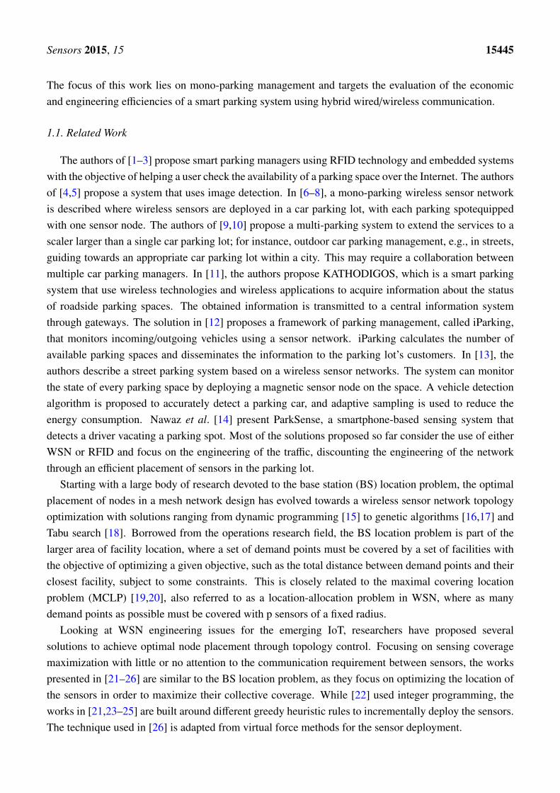
The smart parking system (SPS) considered in this paper was built around a sensor-based method anddesigned based on a multi-layer framework to enable modularity and scalability and to provide differentservices to different users of a parking system. The framework depicted by Figure 1 includes four layers:a sensing, networking, middleware and application layer.

Figure 1. The smart parking system.

Sensors 2015, 15 15448

2.1.1. The Sensing Layer

This layer defines a platform where sensor devices are embedded into the parking lot to detect carpresence/absence, and RFID devices located at the parking gates and strategic points of the parking areused to identify cars based on a unique mapping between RFID tags and cars. Three types of sensordevices are used: (1) slave devices, also called “receivers”, which are placed on the parking spots todetect presence/absence; (2) master devices, also called “transmitters”, which are tasked to collect thesensor readings from their connected slave devices and transmit these readings to a gateway for furtherprocessing; and (3) “anchor” devices used as repeaters to increase the wireless sensor coverage of theparking for efficient routing of the sensor readings. The slave devices are connected to the master devicesthrough wired communication using the I2Cprotocol. For sensing purposes, micro-controllers equippedwith ultrasonic sensors were used, and an ARM-based Panda board was used as the gateway.

2.1.2. The Networking Layer

Different modes of communication have been proposed in this layer to support communication fromthe master and anchor sensors to the sensor gateway and from the gateway to the parking users (parkingdrivers, remote users and parking owners). These include (1) the 802.15.4/ZigBee communication forrouting the sensor readings from master sensors to the gateway, (2) TCP/IP over Ethernet for connectingthe gateway to the parking server and database and (3) Internet access for remote access to the smartparking system from outside.

2.1.3. The Middleware Layer

This layer is the layer where situation recognition is performed using intelligent algorithms andefficient visualization techniques to present smart services and a user-friendly interface to the users.This layer hosts different databases and associated servers and manages all of the software intelligenceprovided by the smart parking system to provide smart services to users by enabling communicationbetween the application layer where services are requested and the lower layers where smart devices areembedded into the parking lot to provide smart services.

2.1.4. The Application Layer

The application layer is the layer where the different services are defined and provided to differentusers. Client devices have been connected via the TCP/IP protocol to a parking database. The latteris updated in real time with the status of the parking lots. Two kinds of client applications have beenconsidered for parking lot monitoring: (1) a mobile device application for phones and tablets; and (2) adesktop application for laptops and desktop computers.

2.2. The Smart Parking Services

The different services provided by our smart parking system include:

Sensors 2015, 15 15449

• Proactive guidance service: In our current implementation, active RFID technology has been usedto replace the paper-based ticketing system and provide drivers’ guidance by enabling car drivers touse their RFID tag in order to be guided toward their pre-allocated parking spot. In this case, RFIDreaders placed at strategic points of the parking lot are used to get the tag’s ID and to interrogate adatabase managed by the parking manager to retrieve the pre-allocated parking spot and guide thedriver. Each vehicle driver is assumed to have been given an active RFID tag.

• Reactive guidance service: When parking spot pre-allocation is not an option, a reactive guidancemodel is used where the parking RFID readers are programmed to retrieve the nearest available(optimal) parking spot from the parking manager. The optimal location is calculated based on thecurrent location of the car and a map of free spots, which is built based on the car presence/absencedetection system and maintained by one of the parking servers.

• Car retrieval service: This service also uses the tag carried by the driver to interrogate the readerslocated in different spots and to transmit the tag’s ID to the parking manager. The latter checks theoccupied parking spots in the database and in the parking lot and returns a response to the parkingguidance node for visualization using a visualization management system (VMS).

• Smart parking regulation: The smart parking regulation takes place when the car drivers have aspecific parking area pre-allocated for their use or when parking spot reservation is implemented.When a car is detected in a parking spot, a presence event, including the RFID tag’s ID of a carand its location, is transmitted to the parking manager. This latter uses the information received tocheck in its database if the identified car is authorized to access the location.

• Parking security services: The current implementation of the SPS enables a driver to be providedeither a permanent RFID tag in the case of a private parking spot or a temporary one at the parkingentrance in the case of a public parking spot. The tag is used for different purposes, includingsecurity purposes through (1) a one-to-one mapping between the RFID tag identifying a car anda parking spot and (2) a security check process where the tag is used to detect car theft when theparking manager software detects a car leaving the parking spot while its corresponding tag issignaled by the closest reader to be far from the identified parking spot.

While the first version of our prototype includes the services described above, many other servicesare planned to be included in our SPS in the near future. These include:

• Parking availability status by integrating into the car detection system sources of light on parkingspots, which are controlled by actuators to inform of the status of a parking spot: e.g., red foroccupied, green for empty, yellow for reserved and blue for out of service.

• Parking payment service to replace the paper-based payment by RFID tags, which are collected atthe parking entrance and used when leaving the parking lot at an RFID-based payment machine tocompute the time spent in the parking lot and subsequently bill the car driver.

• Parking gate management to enable gates to be opened automatically to enable an authorizeddriver access to a specific part of the the parking lot. This service is similar to the smart parkingregulation service, as they are both built around an authorization system aimed to constrain accessbased on permissions.

Sensors 2015, 15 15450

• Remote availability checking using the Internet and/or the GSM network to check in real time theavailability of the smart parking system. By enabling access to a smart parking availability status“anytime” and “anywhere”, this service can provide substantial time savings for a parking user.

2.3. Implementation Challenges

The design and implementation of the smart parking system described above has raised severalchallenges. Some have been addressed during the prototype implementation at CERIST, while othershave been reserved for future research work.

• Sensor selection: The selection of the appropriate sensing technology is a challenging issue uponwhich the efficiency of a smart parking deployment depends. Size, reliability, adaptation toenvironmental changes, robustness and cost are among the parameters that usually play a keyrole when selecting the type of sensors for a smart parking system. Furthermore, intrusive sensors,which need to be installed directly on the pavement surface, are usually avoided, as they havea number of challenges, including the need for digging and tunneling under the road surface.Ultrasonic sensors were considered in our deployment, as they were low cost and required simpleinstallation by being fixed on the ground.

• I2C protocol issues: One of the main challenges was to alter the I2C for our application, given thatthe it has not been designed to operate at long distances. Some changes to some I2C parametershave been necessary, such as the pull resistance and clock frequency.

• Power supply issues: Another challenge was the power supply connection for all of the sensormotes with efficient power consumption.

• Potential imperfections: When deployed outdoors, ultrasonic sensors are known to be sensitive totemperature changes and extreme air turbulence. Potential imperfections associated with indoorwireless communication, such as interference, reflection, diffraction and wall penetration, arechallenges that will have to be dealt with when deploying the SPS indoor.

• Efficient wireless coverage: For both indoor and outdoor deployment, the efficient wirelesscoverage is an important parameter upon which the lifetime of the smart parking system depends.This is the main issue addressed in this paper.

3. The Optimal Sensor Placement Model

Figure 2 depicts the layout of a smart parking system where sensors are organized into islandsof heterogeneous devices (slave sensors, master sensors and repeater/anchor sensors), which areinterconnected by either wired links using I2C and Ethernet protocols or wireless links operating the802.15.4/Zigbee protocol. In such a heterogeneous environment, the slave sensor nodes are located onthe parking spots to detect car presence/absence and report to a master sensor node, while the mastersensor nodes are located at the edge of the parking lot and tasked to report the sensor readings to thegateway where further processing is performed.

The master and slave sensors are located in the parking lot based on geolocation constraints, whichcan lead to poor coverage and the inability for the sensor readings to reach the gateway located at theentrance of the parking lot. Repeater nodes, also referred to as “anchor” nodes, are integrated into the

Sensors 2015, 15 15451

smart parking system to mitigate this issue by strategically placing these sensors at optimally-computedlocations to increase the sensor network coverage and connectivity. As deployed in the smart parkinglot, the slave and master nodes form the edge of the wireless sensor network, while the anchor nodesconstitute the backbone of the sensor network.

Figure 2. The smart parking sensor placement.

3.1. A Multi-Objective Optimization Problem

The optimal placement of anchor nodes in the smart parking system may impact not only the system’sengineering efficiency in terms of efficient data collection and on-time delivery to the gateway, but alsothe economic gain expressed in terms of the number of sensors that are required for monitoring theparking area, as this reflects the financial cost of the deployment. As generally formulated, the optimalnode placement in networks consists of determining the position of nodes that minimizes/maximizesa pre-defined penalty/reward function subject to a set of specifications and/or constraints for a givendeployment area to be covered. The optimal node placement has been widely applied to both base station(BS) location in cellular networks and sensor placement in wireless sensor networks. However, sensornetwork and BS placement problems differ in many aspects, since, while the BS placement problem doesnot require BS connectivity, the optimal sensor placement requires connectivity between sensors to allowmulti-hop dissemination of the readings of all sensors to a unique gateway, where further processing isperformed, as suggested by the traditional one-to-m sensor deployment model.

While many works have resulted in simplifications leading to single objective formulations, theoptimal node placement in a WSN is widely known as a multi-objective optimization problem involvingcompeting objectives, such as coverage and lifetime maximization, with coverage maximizationdegrading lifetime performance, while lifetime maximization reduces WSN coverage. This can beillustrated by the typical “conference room”, scenario where the more close to each other the participantsare, the less energy they will spend for communication (they are maximizing the lifetime of the meeting),while being close to each other results in covering less space in the room (minimize coverage). Inversely,though increasing coverage, scattering the conference participants in a room by having longer average

Sensors 2015, 15 15452

distance between them leads to higher energy consumption for communication (reduction of the lifetimeof the meeting). In a mathematical formulation for node placement in WSN, “scattering” translates intocoverage maximization, while “closeness” is mapped to lifetime maximization expressed by distanceminimization or equivalently min used distance maximization. Furthermore, as suggested by [29],deploying sensors based on a single objective may lead to problems, such as (1) a disconnected networkwhen the sensing range is of the same order or larger than the communication range, as is the case forseismic sensors; and (2) a partition of the WSN if the areas to be covered are disjoint.

3.2. Mathematical Formulation

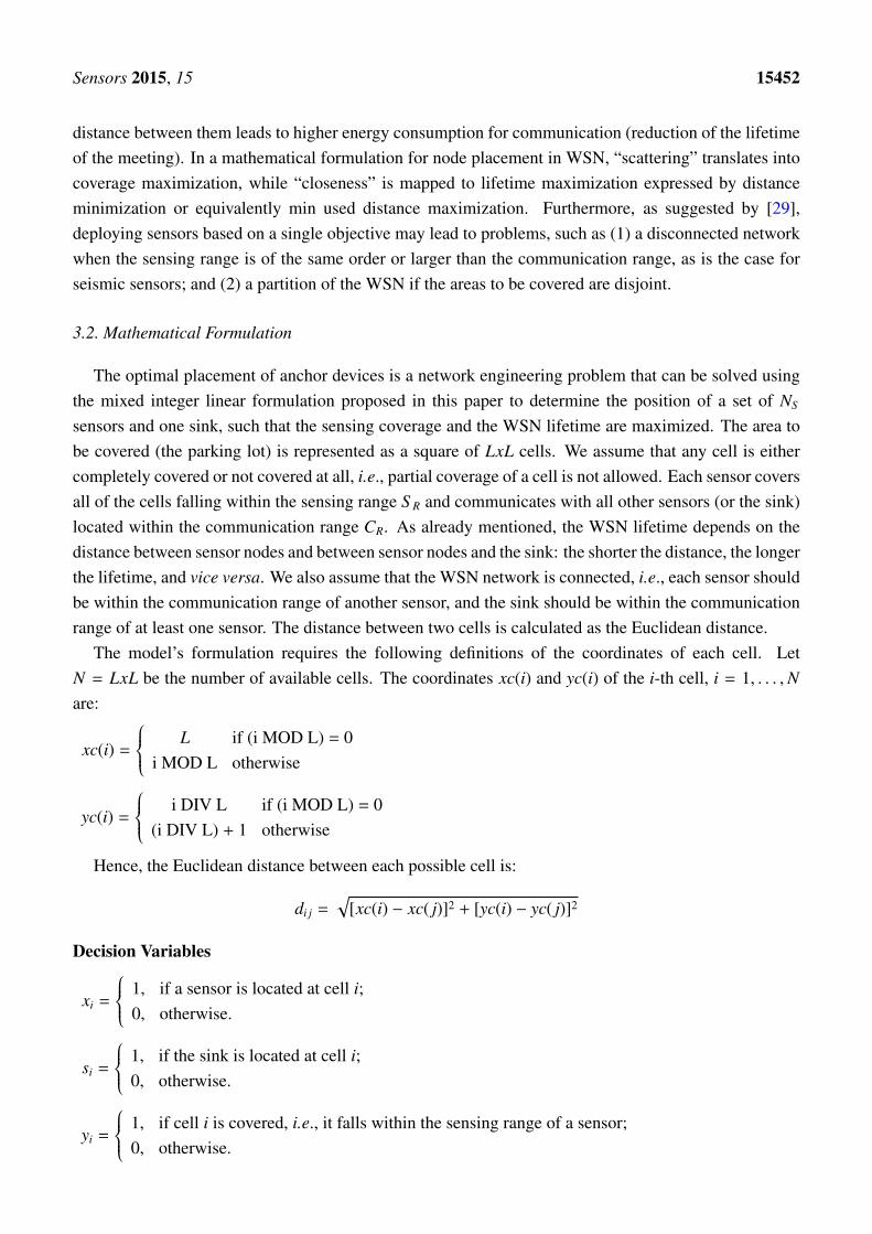
The optimal placement of anchor devices is a network engineering problem that can be solved usingthe mixed integer linear formulation proposed in this paper to determine the position of a set of NS

sensors and one sink, such that the sensing coverage and the WSN lifetime are maximized. The area tobe covered (the parking lot) is represented as a square of LxL cells. We assume that any cell is eithercompletely covered or not covered at all, i.e., partial coverage of a cell is not allowed. Each sensor coversall of the cells falling within the sensing range S R and communicates with all other sensors (or the sink)located within the communication range CR. As already mentioned, the WSN lifetime depends on thedistance between sensor nodes and between sensor nodes and the sink: the shorter the distance, the longerthe lifetime, and vice versa. We also assume that the WSN network is connected, i.e., each sensor shouldbe within the communication range of another sensor, and the sink should be within the communicationrange of at least one sensor. The distance between two cells is calculated as the Euclidean distance.

The model’s formulation requires the following definitions of the coordinates of each cell. LetN = LxL be the number of available cells. The coordinates xc(i) and yc(i) of the i-th cell, i = 1, . . . ,Nare:

xc(i) =

L if (i MOD L) = 0i MOD L otherwise

yc(i) =

i DIV L if (i MOD L) = 0(i DIV L) + 1 otherwise

Hence, the Euclidean distance between each possible cell is:

di j =√

[xc(i) − xc( j)]2 + [yc(i) − yc( j)]2

Decision Variables

xi =

1, if a sensor is located at cell i;0, otherwise.

si =

1, if the sink is located at cell i;0, otherwise.

yi =

1, if cell i is covered, i.e., it falls within the sensing range of a sensor;0, otherwise.

Sensors 2015, 15 15453

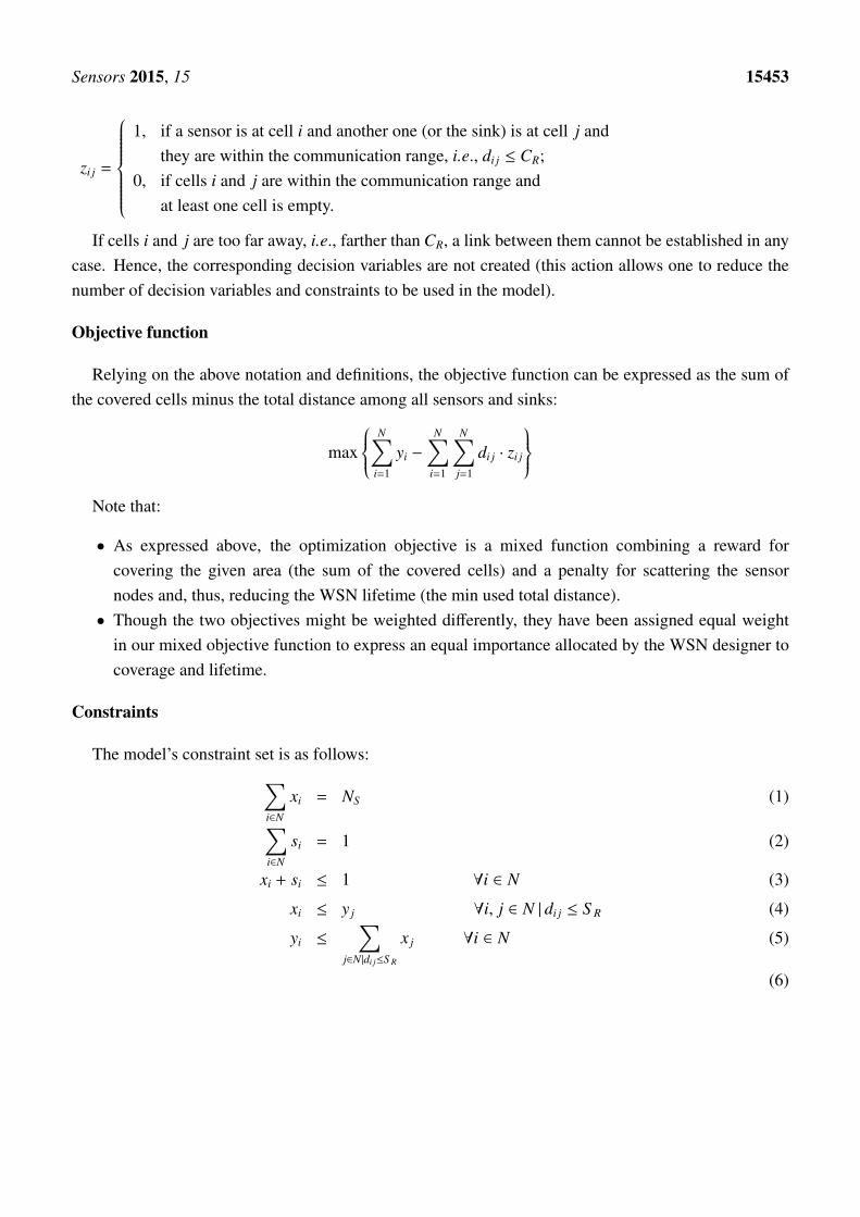
zi j =

1, if a sensor is at cell i and another one (or the sink) is at cell j and

they are within the communication range, i.e., di j ≤ CR;0, if cells i and j are within the communication range and

at least one cell is empty.

If cells i and j are too far away, i.e., farther than CR, a link between them cannot be established in anycase. Hence, the corresponding decision variables are not created (this action allows one to reduce thenumber of decision variables and constraints to be used in the model).

Objective function

Relying on the above notation and definitions, the objective function can be expressed as the sum ofthe covered cells minus the total distance among all sensors and sinks:

max

N∑i=1

yi −

N∑i=1

N∑j=1

di j · zi j

Note that:

• As expressed above, the optimization objective is a mixed function combining a reward forcovering the given area (the sum of the covered cells) and a penalty for scattering the sensornodes and, thus, reducing the WSN lifetime (the min used total distance).

• Though the two objectives might be weighted differently, they have been assigned equal weightin our mixed objective function to express an equal importance allocated by the WSN designer tocoverage and lifetime.

Constraints

The model’s constraint set is as follows:∑i∈N

xi = NS (1)∑i∈N

si = 1 (2)

xi + si ≤ 1 ∀i ∈ N (3)

xi ≤ y j ∀i, j ∈ N | di j ≤ S R (4)

yi ≤∑

j∈N|di j≤S R

x j ∀i ∈ N (5)

(6)

Sensors 2015, 15 15454

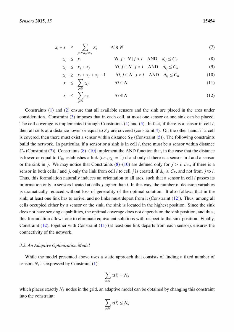
xi + si ≤∑

j∈N|di j≤CR

x j ∀i ∈ N (7)

zi j ≤ xi ∀i, j ∈ N | j > i AND di j ≤ CR (8)

zi j ≤ x j + s j ∀i, j ∈ N | j > i AND di j ≤ CR (9)

zi j ≥ xi + x j + s j − 1 ∀i, j ∈ N | j > i AND di j ≤ CR (10)

xi ≤∑j∈N

zi j ∀i ∈ N (11)

si ≤∑j∈N

z ji ∀i ∈ N (12)

Constraints (1) and (2) ensure that all available sensors and the sink are placed in the area underconsideration. Constraint (3) imposes that in each cell, at most one sensor or one sink can be placed.The cell coverage is implemented through Constraints (4) and (5). In fact, if there is a sensor in cell i,then all cells at a distance lower or equal to S R are covered (constraint 4). On the other hand, if a cellis covered, then there must exist a sensor within distance S R (Constraint (5)). The following constraintsbuild the network. In particular, if a sensor or a sink is in cell i, there must be a sensor within distanceCR (Constraint (7)). Constraints (8)–(10) implement the AND function that, in the case that the distanceis lower or equal to CR, establishes a link (i.e., zi j = 1) if and only if there is a sensor in i and a sensoror the sink in j. We may notice that Constraints (8)–(10) are defined only for j > i, i.e., if there is asensor in both cells i and j, only the link from cell i to cell j is created, if di j ≤ CR, and not from j to i.Thus, this formulation naturally induces an orientation to all arcs, such that a sensor in cell i passes itsinformation only to sensors located at cells j higher than i. In this way, the number of decision variablesis dramatically reduced without loss of generality of the optimal solution. It also follows that in thesink, at least one link has to arrive, and no links must depart from it (Constraint (12)). Thus, among allcells occupied either by a sensor or the sink, the sink is located in the highest position. Since the sinkdoes not have sensing capabilities, the optimal coverage does not depends on the sink position, and thus,this formulation allows one to eliminate equivalent solutions with respect to the sink position. Finally,Constraint (12), together with Constraint (11) (at least one link departs from each sensor), ensures theconnectivity of the network.

3.3. An Adaptive Optimization Model

While the model presented above uses a static approach that consists of finding a fixed number ofsensors Ns as expressed by Constraint (1): ∑

i∈N

x(i) = NS

which places exactly NS nodes in the grid, an adaptive model can be obtained by changing this constraintinto the constraint: ∑

i∈N

x(i) ≤ NS

Sensors 2015, 15 15455

which requires the number of nodes NS to be large enough to meet the sensor placement constraint.Such a change will lead to a model that will adaptively/automatically find the best number of sensorsthat maximize our objective function. It is expected that this will lead to finding the best configurationin fewer runs of the algorithm.

3.4. The Exact Model Solver

As expressed above, the mathematical model is an integer linear programming problem that can besolved using either exact methods or approximative methods based on heuristics, such as those borrowedfrom the evolutionary computation field [36].

Building on the Mosel language widely used to solve linear, integer and quadratic programmingproblems based on the the Xpress-Optimizer library [37], we propose two different solution models forthe multi-objective optimization problem: (1) a single-step solution that considers a multi-constrainedsingle objective optimization problem that integrates the coverage and lifetime objectives into oneobjective subject to the constraints as expressed by the mathematical formulation above; and (2) atwo-step or lexicographic solution, where one of the objectives (maximum coverage) is solved first tofind a solution space that is searched for a solution that solves the second objective (minimum distanceor maximum lifetime). As currently implemented, the Xpress suite includes extension modules thatprovide access to the other solvers, such as (1) a nonlinear programming solver named “Xpress-SLP”;(2) a stochastic modeling engine referred to as “Xpress-SP” and (3) a constraint programming solvercalled “Xpress-Kalis”.

4. Performance Evaluation

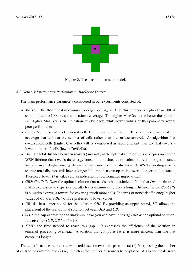
We conducted a set of experiments to analyze the case of a squared shape area of 10 × 10 cells to beoptimally covered by a variable number of sensors with the objective of maximizing coverage and WSNlifetime as expressed by the model formulation in Section 2. Our expectation was to find an optimalnumber of anchor/repeater sensors in a parking lot that could increase the coverage and connectivityof a smart parking system where slave and master sensors have been placed based on application andgeographic constraints. We set the sensing range S R equal to two in terms of Euclidean distance. Thus,each sensor can cover at maximum 13 cells. This is illustrated by Figure 3, where we can see that thegreen cells are those covered if there is a sensor located in the pink cell. It is also assumed that a sensorcovers its cell. The communication range CR is set equal to four in terms of Euclidean distance.

We consider the case where the optimal placement has been designed for (1) a hybrid wired-wirelessbackbone for smart parking and (2) a wireless backbone for smart parking. In the hybrid deployment,a set of hybrid sensor/RFID nodes are placed in a smart parking lot to serve as a backbone for a wiredsensor network, which uses I2C to link ultra-sonic sensors as slaves of the hybrid nodes. In the wirelessdeployment, a set of hybrid nodes are placed in the smart parking lot to serve as a backbone for sensormotes located on the parking spots.

Sensors 2015, 15 15456

Figure 3. The sensor placement model.

4.1. Network Engineering Performance: Backbone Design

The main performance parameters considered in our experiments consisted of:

• MaxCov: the theoretical maximum coverage, i.e., NS ∗ 13. If this number is higher than 100, itshould be set to 100 to express maximal coverage. The higher MaxCovis, the better the solutionis. Higher MaxCov is an indication of efficiency, while lower values of this parameter revealpoor performance.

• CovCells: the number of covered cells by the optimal solution. This is an expression of thecoverage that looks at the number of cells rather than the surface covered. An algorithm thatcovers more cells (higher CovCells) will be considered as more efficient than one that covers alower number of cells (lower CovCells).

• Dist: the total distance between sensors (and sink) in the optimal solution. It is an expression of theWSN lifetime that reveals the energy consumption, since communication over a longer distanceleads to much higher energy depletion than over a shorter distance. A WSN operating over ashorter total distance will have a longer lifetime than one operating over a longer total distance.Therefore, lower Dist values are an indication of performance improvement.

• OBJ: CovCells-Dist: the optimal solution that needs to be maximized. Note that Dist is min usedin this expression to express a penalty for communicating over a longer distance, while CovCellsis plusedto express a reward for covering much more cells. In terms of network efficiency, highervalues of CovCells-Dist will be preferred to lower values.

• UB: the best upper bound for the solution OBJ. By providing an upper bound, UB allows theplacement of the real optimal solution between OBJ and UB.

• GAP: the gap expressing the maximum error you can have in taking OBJ as the optimal solution.It is given by (UB/OBJ − 1) ∗ 100.

• TIME: the time needed to reach this gap. It expresses the efficiency of the solution interms of processing overhead. A solution that computes faster is more efficient than one thatcomputes longer.

These performance metrics are evaluated based on two main parameters: (1) N expressing the numberof cells to be covered; and (2) NS , which is the number of sensors to be placed. All experiments were

Sensors 2015, 15 15457

performed using Xpress Mosel 64-bit v3.2.0 and Xpress optimizer Version 20.00.11 on a Intel XEONwith 16 CPUs at 2.27 GHz and with 16.00Gb of RAM.

4.1.1. The Static Solution

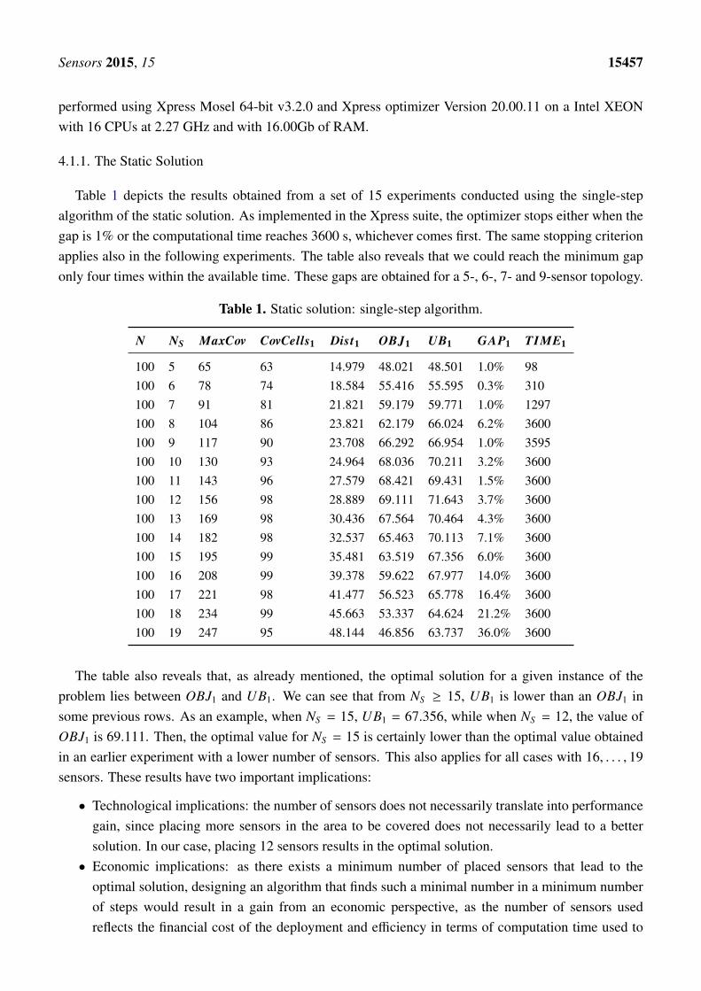
Table 1 depicts the results obtained from a set of 15 experiments conducted using the single-stepalgorithm of the static solution. As implemented in the Xpress suite, the optimizer stops either when thegap is 1% or the computational time reaches 3600 s, whichever comes first. The same stopping criterionapplies also in the following experiments. The table also reveals that we could reach the minimum gaponly four times within the available time. These gaps are obtained for a 5-, 6-, 7- and 9-sensor topology.

Table 1. Static solution: single-step algorithm.

N NS MaxCov CovCells1 Dist1 OBJ1 UB1 GAP1 TIME1

100 5 65 63 14.979 48.021 48.501 1.0% 98100 6 78 74 18.584 55.416 55.595 0.3% 310100 7 91 81 21.821 59.179 59.771 1.0% 1297100 8 104 86 23.821 62.179 66.024 6.2% 3600100 9 117 90 23.708 66.292 66.954 1.0% 3595100 10 130 93 24.964 68.036 70.211 3.2% 3600100 11 143 96 27.579 68.421 69.431 1.5% 3600100 12 156 98 28.889 69.111 71.643 3.7% 3600100 13 169 98 30.436 67.564 70.464 4.3% 3600100 14 182 98 32.537 65.463 70.113 7.1% 3600100 15 195 99 35.481 63.519 67.356 6.0% 3600100 16 208 99 39.378 59.622 67.977 14.0% 3600100 17 221 98 41.477 56.523 65.778 16.4% 3600100 18 234 99 45.663 53.337 64.624 21.2% 3600100 19 247 95 48.144 46.856 63.737 36.0% 3600

The table also reveals that, as already mentioned, the optimal solution for a given instance of theproblem lies between OBJ1 and UB1. We can see that from NS ≥ 15, UB1 is lower than an OBJ1 insome previous rows. As an example, when NS = 15, UB1 = 67.356, while when NS = 12, the value ofOBJ1 is 69.111. Then, the optimal value for NS = 15 is certainly lower than the optimal value obtainedin an earlier experiment with a lower number of sensors. This also applies for all cases with 16, . . . , 19sensors. These results have two important implications:

• Technological implications: the number of sensors does not necessarily translate into performancegain, since placing more sensors in the area to be covered does not necessarily lead to a bettersolution. In our case, placing 12 sensors results in the optimal solution.

• Economic implications: as there exists a minimum number of placed sensors that lead to theoptimal solution, designing an algorithm that finds such a minimal number in a minimum numberof steps would result in a gain from an economic perspective, as the number of sensors usedreflects the financial cost of the deployment and efficiency in terms of computation time used to

Sensors 2015, 15 15458

find the optimal placement of sensors. This implication has resulted in the “adaptive” version ofthe algorithm previously described in Section 3.3 and discussed later in this section.

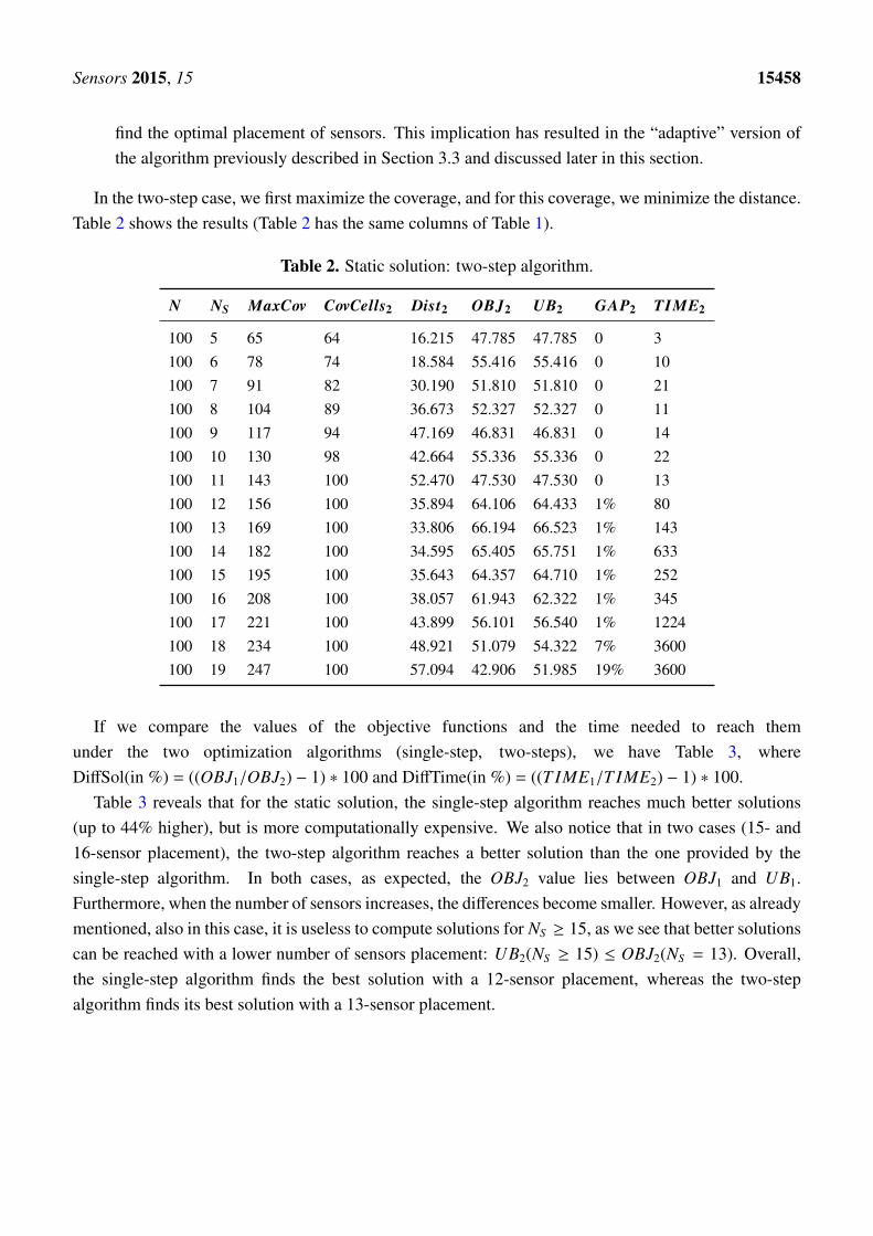
In the two-step case, we first maximize the coverage, and for this coverage, we minimize the distance.Table 2 shows the results (Table 2 has the same columns of Table 1).

Table 2. Static solution: two-step algorithm.

N NS MaxCov CovCells2 Dist2 OBJ2 UB2 GAP2 TIME2

100 5 65 64 16.215 47.785 47.785 0 3100 6 78 74 18.584 55.416 55.416 0 10100 7 91 82 30.190 51.810 51.810 0 21100 8 104 89 36.673 52.327 52.327 0 11100 9 117 94 47.169 46.831 46.831 0 14100 10 130 98 42.664 55.336 55.336 0 22100 11 143 100 52.470 47.530 47.530 0 13100 12 156 100 35.894 64.106 64.433 1% 80100 13 169 100 33.806 66.194 66.523 1% 143100 14 182 100 34.595 65.405 65.751 1% 633100 15 195 100 35.643 64.357 64.710 1% 252100 16 208 100 38.057 61.943 62.322 1% 345100 17 221 100 43.899 56.101 56.540 1% 1224100 18 234 100 48.921 51.079 54.322 7% 3600100 19 247 100 57.094 42.906 51.985 19% 3600

If we compare the values of the objective functions and the time needed to reach themunder the two optimization algorithms (single-step, two-steps), we have Table 3, whereDiffSol(in %) = ((OBJ1/OBJ2) − 1) ∗ 100 and DiffTime(in %) = ((T IME1/T IME2) − 1) ∗ 100.

Table 3 reveals that for the static solution, the single-step algorithm reaches much better solutions(up to 44% higher), but is more computationally expensive. We also notice that in two cases (15- and16-sensor placement), the two-step algorithm reaches a better solution than the one provided by thesingle-step algorithm. In both cases, as expected, the OBJ2 value lies between OBJ1 and UB1.Furthermore, when the number of sensors increases, the differences become smaller. However, as alreadymentioned, also in this case, it is useless to compute solutions for NS ≥ 15, as we see that better solutionscan be reached with a lower number of sensors placement: UB2(NS ≥ 15) ≤ OBJ2(NS = 13). Overall,the single-step algorithm finds the best solution with a 12-sensor placement, whereas the two-stepalgorithm finds its best solution with a 13-sensor placement.

Sensors 2015, 15 15459

Table 3. Comparing static algorithms.

NS DiffSol (in %) DiffTime (in %)

5 0.5% 2844%6 0.0% 2856%7 14.2% 6140%8 18.8% 32,328%9 41.6% 25,181%

10 23.0% 15,612%11 44.0% 28,370%12 7.8% 4375%13 2.1% 2424%14 0.1% 469%15 –1.3% 1326%16 –3.7% 943%17 0.8% 194%18 4.4% 0%19 9.2% 0%

4.1.2. The Adaptive Model

We conducted another set of experiments using the two algorithms (single-step and two-step) by fixinga bound to the number of nodes (a large number equal to 20 in our case) to find opportunistically theoptimal configurations in terms of number of nodes found by the two algorithms. Thus, our formulationallows one to identify the best configuration both in terms of (1) the number of sensors and (2) theposition of sensors with the objective of maximizing the trade-off between sensing coverage and lifetimeexpressed by the total distance.

Our experimental results presented in Table 4 revealed that in both cases, the best configurationsresult in 12 sensors in the single-step case and 13 sensors in the two-step case when using the sameobjective function value in both cases. These results are in agreement with the static solution, but withthe advantage of a faster implementation requiring just one run per case.

The results depicted in Table 4 above reveal that using the two-step approach, we reach the optimalsolution in much less time than the maximum allowed time (3600 s). On the other hand, the single-stepalgorithm provides better value of CovCells-Dist with 12 sensors. This appeals to a trade-off between thequality of the solution and computation time, which depends on the algorithm’s use: while computationalcomplexity is not a concern in the preemptive algorithms used during the planning phase of a WSN, it isa great concern in proactive algorithms that aim to repair a WSN configuration after planning. The studyof such a tradeoff is beyond the scope of this paper.

Figure 4 depicts the two topologies generated by the optimized solution when using the single-stepand two-steps algorithms. The figure reveals a difference not only in the sink (red dot) and normalnode (blue dot) placement, but also a difference in the zones of possible interference depicted by theshaded areas.

Sensors 2015, 15 15460

Table 4. Comparing adaptive algorithms.

Parameters Single-Step Two-Steps

NS 12 13CovCells 98 100Dist 28.889 33.806OBJ 69.111 66.194Upper Bound 70.988 66.532Gap 2.7% 1%Time 3600 s 1635 s

(a) (b)

Figure 4. Optimized Topologies Comparison. (a) Single-step Generated Topology;(b) Two-steps Generated Topology.

4.2. Traffic Engineering Performance: Wireless Communication

Another set of experiments was conducted to evaluate the traffic engineering performance of thewireless backbone design using two types of network configurations: (1) a random network configurationdesigned using the K-connectivity algorithm to place the sensors in the network to achieve coverage andone-connectivity; and (2) an optimized network configuration designed using the single-step algorithmto generate a backbone network of anchor nodes for a set of pre-established slave and master nodes, asproposed in this paper. Following the modeling and performance analysis approach used in [38,39], weevaluated the performance of the two network configurations when using different routing algorithmsto move the sensor readings from nodes to the sink node of the smart parking sensor network. Thesealgorithms include (1) the energy-constrained multipath (ECMP) and the multi-constrained multipath(MCMP) routing algorithms; (2) the ad hoc on-demand (AODV) single-path algorithm and (3) thelink-disjoint multipath routing (LDPR) algorithm.

Sensors 2015, 15 15461

4.2.1. Performance Parameters

We considered three main performance parameters: (1) the average energy consumption for differentdelay requirements; (2) the average playback delay for different delay requirements; and (3) theaverage packet delivery for different delay requirements. The packet delivery is defined by the ratioof packets successfully delivered to the destination over the total number of transmitted packets. Thepath delayD(p), that is the delay between a node and the sink, is given by the sum of link delays:

D(p) =∑`∈p

d` (13)

where d` is the delay of data over the link `. The playback delay is the delay taken to deliver the packetsfrom one source to the sink (destination) in a multipath setting. It is the time taken to deliver the packetsfrom the first one to the last one. It is mathematically defined by:

D(P(s, d)) = maxp∈P(s,d)

D(p) (14)

where P(s, d) is the set of parallel paths between source s and destination d. Similarly, the path energyis expressed by the sum of the energies expanded over the links of the path. It is expressed by:

W`(p) =∑`∈p

w` (15)

where w` is the energy expanded on link ` expressed by:

w` = f` · w(si, si+1) (16)

where f` is the data rate on link ` and w(si, si+1) is the power required by the source node si on link `to receive a bit of data and then transmit it to the destination node si+1. As defined by the energy modelin [39], w(si, si+1) is expressed by:

w(si, si+1) = α1 + α2|| xsi − xsi+1 ||n (17)

where α1 = α11 + α12 with α11 being the energy per bit consumed by si as the transmitter, α12 theenergy per bit consumed as the receiver and α2 accounting for the energy dissipated (link loss) duringtransmission. Typical values for α1 and α2 are, respectively, α11 = 180 nJ/bit and α2 = 10 pJ/bit/m2 forthe link loss experienced by a radio transmission when n = 2 or α2 = 0.001 pJ/bit/m4 for the link lossexperienced by a radio transmission when n = 4. xsi and xsi+1 are the locations of the sensor nodes si andsi+1, respectively, while || xsi − xsi+1 || is the Euclidean distance between the two sensor nodes.

4.2.2. Average Energy Consumption

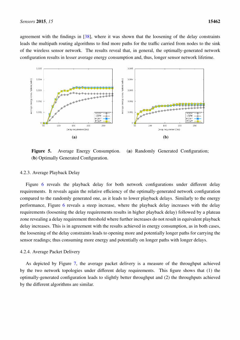
Figure 5 reveals the energy consumption for both network configurations under different delayrequirements. It reveals an energy consumption patterns with a steep increase followed by a plateaufor all of the algorithms. The steep increase reveals a network operation zone where loosening thedelay requirements leads to higher energy consumption, while the plateau reveals a delay thresholdwhere further increases do not translate into equivalent energy consumption. The steep increase is in

Sensors 2015, 15 15462

agreement with the findings in [38], where it was shown that the loosening of the delay constraintsleads the multipath routing algorithms to find more paths for the traffic carried from nodes to the sinkof the wireless sensor network. The results reveal that, in general, the optimally-generated networkconfiguration results in lesser average energy consumption and, thus, longer sensor network lifetime.

(a) (b)

Figure 5. Average Energy Consumption. (a) Randomly Generated Configuration;(b) Optimally Generated Configuration.

4.2.3. Average Playback Delay

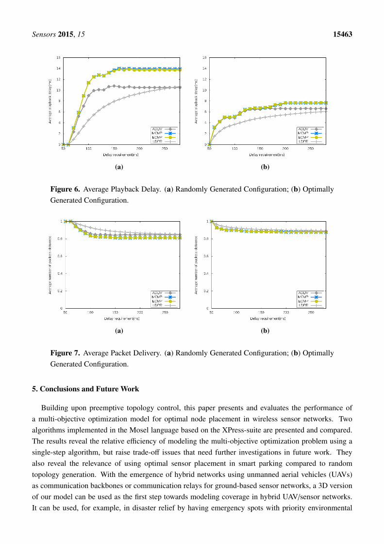
Figure 6 reveals the playback delay for both network configurations under different delayrequirements. It reveals again the relative efficiency of the optimally-generated network configurationcompared to the randomly generated one, as it leads to lower playback delays. Similarly to the energyperformance, Figure 6 reveals a steep increase, where the playback delay increases with the delayrequirements (loosening the delay requirements results in higher playback delay) followed by a plateauzone revealing a delay requirement threshold where further increases do not result in equivalent playbackdelay increases. This is in agreement with the results achieved in energy consumption, as in both cases,the loosening of the delay constraints leads to opening more and potentially longer paths for carrying thesensor readings; thus consuming more energy and potentially on longer paths with longer delays.

4.2.4. Average Packet Delivery

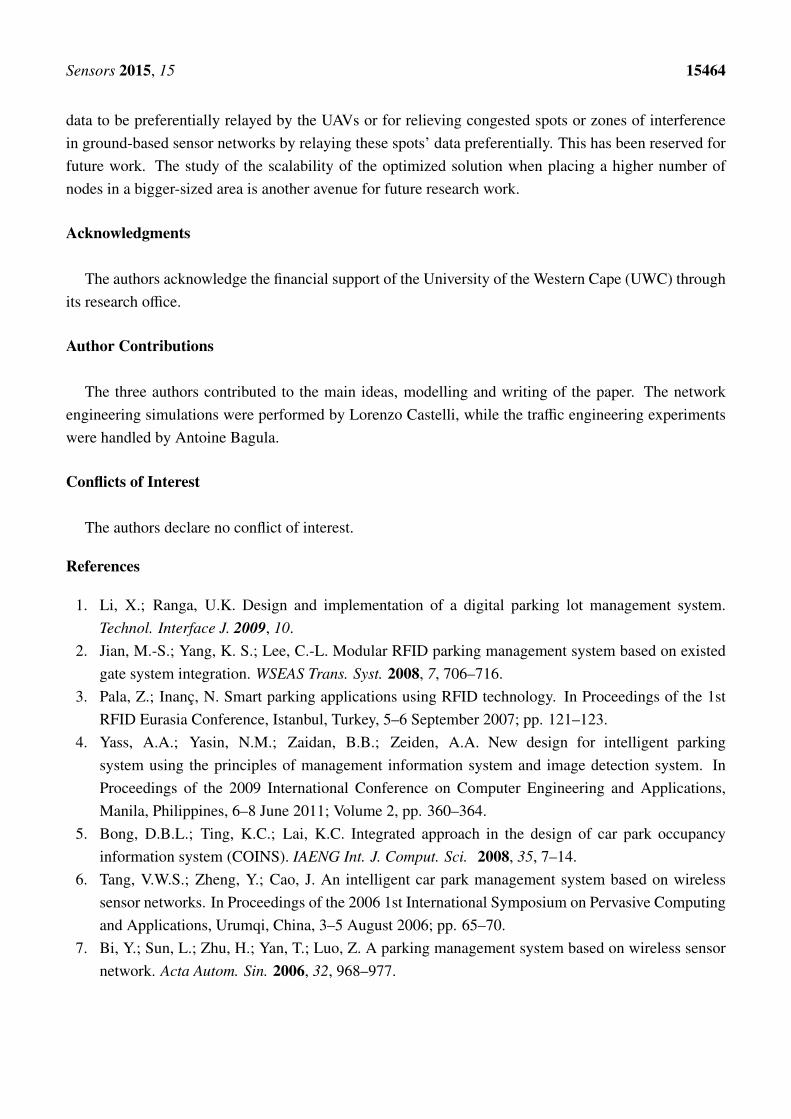
As depicted by Figure 7, the average packet delivery is a measure of the throughput achievedby the two network topologies under different delay requirements. This figure shows that (1) theoptimally-generated configuration leads to slightly better throughput and (2) the throughputs achievedby the different algorithms are similar.

Sensors 2015, 15 15463

(a) (b)

Figure 6. Average Playback Delay. (a) Randomly Generated Configuration; (b) OptimallyGenerated Configuration.

(a) (b)

Figure 7. Average Packet Delivery. (a) Randomly Generated Configuration; (b) OptimallyGenerated Configuration.

5. Conclusions and Future Work

Building upon preemptive topology control, this paper presents and evaluates the performance ofa multi-objective optimization model for optimal node placement in wireless sensor networks. Twoalgorithms implemented in the Mosel language based on the XPress-suite are presented and compared.The results reveal the relative efficiency of modeling the multi-objective optimization problem using asingle-step algorithm, but raise trade-off issues that need further investigations in future work. Theyalso reveal the relevance of using optimal sensor placement in smart parking compared to randomtopology generation. With the emergence of hybrid networks using unmanned aerial vehicles (UAVs)as communication backbones or communication relays for ground-based sensor networks, a 3D versionof our model can be used as the first step towards modeling coverage in hybrid UAV/sensor networks.It can be used, for example, in disaster relief by having emergency spots with priority environmental

Sensors 2015, 15 15464

data to be preferentially relayed by the UAVs or for relieving congested spots or zones of interferencein ground-based sensor networks by relaying these spots’ data preferentially. This has been reserved forfuture work. The study of the scalability of the optimized solution when placing a higher number ofnodes in a bigger-sized area is another avenue for future research work.

Acknowledgments

The authors acknowledge the financial support of the University of the Western Cape (UWC) throughits research office.

Author Contributions

The three authors contributed to the main ideas, modelling and writing of the paper. The networkengineering simulations were performed by Lorenzo Castelli, while the traffic engineering experimentswere handled by Antoine Bagula.

Conflicts of Interest

The authors declare no conflict of interest.

References

1. Li, X.; Ranga, U.K. Design and implementation of a digital parking lot management system.Technol. Interface J. 2009, 10.

2. Jian, M.-S.; Yang, K. S.; Lee, C.-L. Modular RFID parking management system based on existedgate system integration. WSEAS Trans. Syst. 2008, 7, 706–716.

3. Pala, Z.; Inanç, N. Smart parking applications using RFID technology. In Proceedings of the 1stRFID Eurasia Conference, Istanbul, Turkey, 5–6 September 2007; pp. 121–123.

4. Yass, A.A.; Yasin, N.M.; Zaidan, B.B.; Zeiden, A.A. New design for intelligent parkingsystem using the principles of management information system and image detection system. InProceedings of the 2009 International Conference on Computer Engineering and Applications,Manila, Philippines, 6–8 June 2011; Volume 2, pp. 360–364.

5. Bong, D.B.L.; Ting, K.C.; Lai, K.C. Integrated approach in the design of car park occupancyinformation system (COINS). IAENG Int. J. Comput. Sci. 2008, 35, 7–14.

6. Tang, V.W.S.; Zheng, Y.; Cao, J. An intelligent car park management system based on wirelesssensor networks. In Proceedings of the 2006 1st International Symposium on Pervasive Computingand Applications, Urumqi, China, 3–5 August 2006; pp. 65–70.

7. Bi, Y.; Sun, L.; Zhu, H.; Yan, T.; Luo, Z. A parking management system based on wireless sensornetwork. Acta Autom. Sin. 2006, 32, 968–977.

Sensors 2015, 15 15465

8. Benson, J.P.; O’Donovan, T.; O’Sullivan, P.; Roedig, U.; Sreenan, C.; Barton, J.; Murphy, A.;O’Flynn, B. Car-park management using wireless sensor networks. In Proceedings of the 200631st IEEE Conference on Local Computer Networks, Tampa, FL, USA, 14–16 November 2006;pp. 588–595.

9. Geng, Y.; Cassandras, C.G. A new ‘smart parking’ system infrastructure and implementation.Procedia–Soc. Behav. Sci. 2012, 54, 1278–1287.

10. Lu, R.; Lin, X.; Zhu, H.; Shen, X. SPARK: A New VANET-based Smart Parking Scheme for LargeParking Lots. In Proceedings of IEEE INFOCOM 2009, Rio de Janeiro, Brazil, 19–25 April 2009;pp. 1413–1421.

11. Samaras, A.; Evangeliou, N.; Arvanitopoulos, A.; Gialelis, J.; Koubias, S.; Tzes, A.KATHODIGOS–A Novel Smart Parking System based on Wireless Sensor Networks. InProceedings of the 1st International Virtual Conference on Intelligent Transportation Systems,Slovakia, 26–30 August 2013; pp. 140–145.

12. Chinrungrueng, J.; Dumnin, S.; Pongthornseri, R. IParking: A parking management framework.In Proceedings of the IEEE 11th International Conference on ITS Telecommunications (ITST),St. Petersburg, Russia, 23–25 August 2011; pp. 63–68.

13. Gu, J.; Zhang, Z.; Yu, F.; Liu, Q. Design and implementation of a street parking system usingwireless sensor networks. In Proceedings of the 10th IEEE International Conference on IndustrialInformatics (INDIN), Beijing, China, 25–27 July 2012; pp. 1212–1217.

14. Nawaz, S.; Efstratiou, C.; Mascolo, C. Parksense: A smartphone based sensing system for on-streetparking. In Proceedings of the 19th Annual International Conference on Mobile Computing andNetworking, Miami, FL, USA, 30 September–4 October 2013; pp. 75–86.

15. Rose, R. A smart technique for determining base-station locations in an urban environment.IEEE Trans. Veh. Technol. 2001, 50, 43–47.

16. Han, J.K.; Park, B.S.; Choi, Y.S.; Park, H.K. Genetic approach with a new representation forbase station placement in mobile communications. In Proceedings of the 2001 IEEE VehicularTechnology Conference, Atlantic City, NJ, USA, 7–11 October 2001; Volume 4, pp. 2703–2707.

17. Meunier, H.; Talbi, E.; Reininger, P. A multiobjective genetic algorithm for radio networkoptimization. In Proceedings of the 2000 Congress on Evolutionary Computation, La Jolla, CA,USA, 16–19 July 2000; Volume 1, pp. 317–324.

18. Amaldi, E.; Capone, A.; Malucelli, F.; Signori, F. UMTS radio planning: Optimizing base stationconfiguration. In Proceedings of the 2002 IEEE Vehicular Technology Conference, Vancouver, BC,Canada, 24–28 September 2002; Volume 2, pp. 768–772.

19. Church, R.; Velle, C.R. The maximal covering location problem. Pap. Reg. Sci. 1974, 32, 101–118.20. Mehzer, A.; Stulman, A. The maximal covering location problem with facility placement on the

entire plane. J. Reg. Sci. 1982, 22, 361–365.21. Bulusu, N.; Heidemann, J.; Estrin, D. Adaptive beacon placement. In Proceedings of the

21st International Conference on Distributed Computing Systems, Mesa, AZ, USA, April 2001;pp. 489–498.

22. Chakrabarty, K.; Iyengar, S.S.; Qi, H.; Cho, E. Grid coverage for surveillance and target locationin distributed sensor networks. IEEE Trans. Comput. 2002, 51, 1448–1453.

Sensors 2015, 15 15466

23. Dhillon, S.S.; Chakrabarty, K.; Iyengar, S.S. Sensor placement for grid coverage under imprecisedetections. In Proceedings of the Fifth International Conference on Information Fusion, Annapolis,MD, USA, 8–11 July 2002; Volume 2, pp. 1581–1587.

24. Howard, A.; Mataric, M.J.; Sukhatme, G.S. An incremental self-deployment algorithm for mobilesensor networks. Auton. Robots 2002, 13, 113–126.

25. Howard, A.; Mataric, M.J.; Sukhatme, G.S. Mobile sensor network deployment using potentialfields: A distributed, scalable solution to the area coverage problem. Distrib. Auton. Robot. Syst.2002, 5, 299–308.

26. Zou, Y.; Chakrabarty, K. Sensor deployment and target localization based on virtual forces.In Proceedings of the Twenty-Second Annual Joint Conference of the IEEE Computer andCommunications Societies (INFOCOM 2003), San Francisco, CA, USA, 30 March–3 April 2003;Volume 2, pp. 1293–1303.

27. Fonseca, C.M.; Fleming, P.J. Genetic algorithms for Multiobjective Optimization: Formulation,Discussion and Generalization. In Proceedings of the Fifth International Conference on GeneticAlgorithms, Urbana-Champaign, IL, USA, 17–22 July 1993; Volume 93, pp. 416–423.

28. Jourdan, D.B.; de Weck, O.L. Layout Optimization for a Wireless Sensor Network Using aMulti-Objective Genetic Algorithm. In Proceedings of the 2004 59th IEEE Vehicular TechnologyConference, Milan, Italy, 17–19 May 2004; Volume 5, pp. 2466–2470.

29. Jourdan, D.B.; de Weck, O.L. Multi-Objective Genetic Algorithm for the Automated Planning of aWireless Sensor Network to Monitor a Critical Facility. In Proceedings of the SPIE, Sensors, andCommand, Control, Communications, and Intelligence (C3I) Technologies for Homeland Securityand Homeland Defense III, Orlando, FL, USA, 12–16 April 2004; Volume 5403, pp. 565–575.

30. Jourdan, D.B.; Roy, N. Optimal sensor placement for agent localization. ACM Trans. Sens. Netw.(TOSN) 2008, 4, 13:1–13:40.

31. Li, W.; Cassandras, C.G. A minimum-power wireless sensor network self-deployment scheme.In Proceedings of the 2005 IEEE Wireless Communications and Networking Conference,New Orleans, LA, USA, 13–17 March 2005; Volume 3, pp. 1897–1902.

32. Biagioni, E.S.; Sasaki, G. Wireless sensor placement for reliable and efficient data collection. InProceedings of the 36th Annual Hawaii International Conference on System Science, Big Island,HI, USA, 6–9 January 2003.

33. Zhang, H.; Hou, J.C. On the upper bound of α-lifetime for large sensor networks. ACM Trans.Sens. Netw. (TOSN) 2005, 1, 272–300.

34. Dhillon, S.S.; Chakrabarty, K. Sensor placement for effective coverage and surveillance indistributed sensor networks. In Proceedings of the 2003 IEEE Wireless Communications andNetworking Conference, New Orleans, LA, USA, 16–20 March 2003; Volume 3, pp. 1609–1614.

35. Djenouri, D.; Karbab, E.; Boulkaboul, S.; Bagula, A. Car Park Management with NetworkedWireless Sensors and Active RFID. In Proceedings of the 2015 IEEE International Conferenceon Electro Information Technology, EIT-2015, Naperville, IL, USA, 23 May 2015.

Sensors 2015, 15 15467

36. Costanzo, S.; Castelli, L.; Turco, A. MOGASI: A multi-objective genetic algorithm for efficientlyhandling constraints and diversified decision variables. In Engineering Optimization; CRC Press:Boca Raton, FL, USA, 2014; pp. 99–104.

37. Xpress-Mosel User Guide, Release 3.2. FICO: San Jose, CA, USA, 2010.38. Bagula, A.B.; Mazandu, K.G. Energy Constrained Multipath Routing in Wireless Sensor Networks.

In Proceedings of the 5th International Conference on Ubiquitous Intelligence and Computing(UIC ’08), Oslo, Norway, 23–25 June 2008; pp. 453–467.

39. Bagula, A.B. Modelling and implementation of QoS in wireless sensor networks:A multiconstrained traffic engineering model. EURASIP J. Wirel. Commun. Netw. 2010,2010, 1–14.

c© 2015 by the authors; licensee MDPI, Basel, Switzerland. This article is an open access articledistributed under the terms and conditions of the Creative Commons Attribution license(http://creativecommons.org/licenses/by/4.0/).