Embed Size (px)
Citation preview
Sensorless Plug-and-Play Control of Industrial DrivesFocus on Induction Motor Drives
Marko Hinkkanen
IEEE SLED 2019, Torino, Italy10 September, 2019
1 / 48

Introduction
V/Hz Control
Observers
Sensorless Identification at Standstill
Sensorless, More or Less
2 / 48
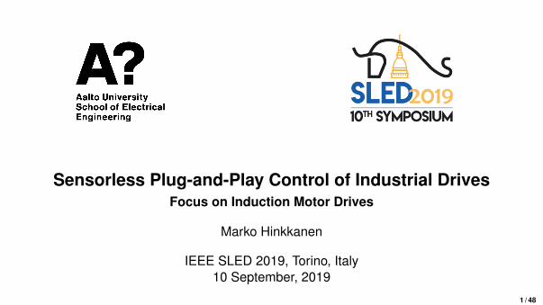
Industry Applications
I Major industry applicationsI Pumps, fans, compressors (> 75%)I ConveyorsI Elevators and escalatorsI Cranes and hoistsI Machine tools, rolling mills, etc.
I Sensorless general-purpose drivesare typically used
I Induction motors dominate (> 90%),but the share of synchronous motorsis increasing
Figure: Google (Hamina data center).3 / 48
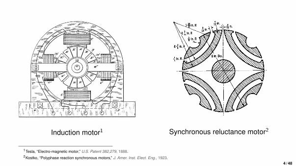
Induction motor1 Synchronous reluctance motor2
1Tesla, “Electro-magnetic motor,” U.S. Patent 382,279, 1888.2Kostko, “Polyphase reaction synchronous motors,” J. Amer. Inst. Elect. Eng., 1923.
4 / 48
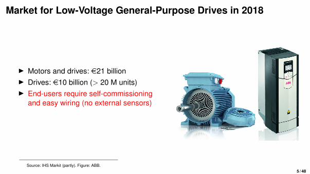
Market for Low-Voltage General-Purpose Drives in 2018
I Motors and drives: e21 billionI Drives: e10 billion (> 20 M units)I End-users require self-commissioning
and easy wiring (no external sensors)
Source: IHS Markit (partly). Figure: ABB.5 / 48
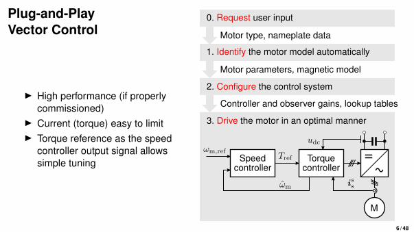
Plug-and-PlayVector Control
I High performance (if properlycommissioned)
I Current (torque) easy to limitI Torque reference as the speed
controller output signal allowssimple tuning
Tref
iss
M
Torquecontroller
udc
Speedcontroller
ωm,ref
ωm
1. Identify the motor model automatically
2. Configure the control system
3. Drive the motor in an optimal manner
Motor parameters, magnetic model
Controller and observer gains, lookup tables
0. Request user input
Motor type, nameplate data
6 / 48

Introduction
V/Hz Control
Observers
Sensorless Identification at Standstill
Sensorless, More or Less
7 / 48
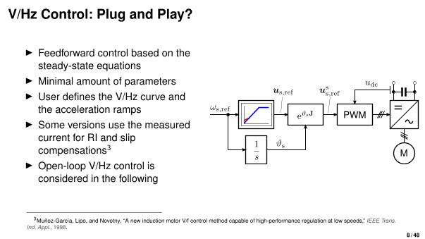
V/Hz Control: Plug and Play?
I Feedforward control based on thesteady-state equations
I Minimal amount of parametersI User defines the V/Hz curve and
the acceleration rampsI Some versions use the measured
current for RI and slipcompensations3
I Open-loop V/Hz control isconsidered in the following
M
uss,ref
ωs,refPWM
udc
eϑsJ
1
s
us,ref
ϑs
3Munoz-Garcıa, Lipo, and Novotny, “A new induction motor V/f control method capable of high-performance regulation at low speeds,” IEEE Trans.Ind. Appl., 1998.
8 / 48
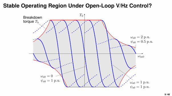
Stable Operating Region Under Open-Loop V/Hz Control?
ωs0 = 1 p.u.ψs0 = 1 p.u.
T0
ωm0
ωs0 = 2 p.u.ψs0 = 0.5 p.u.
Breakdown
ωs0 = 0ψs0 = 1 p.u.
torque Tb
9 / 48
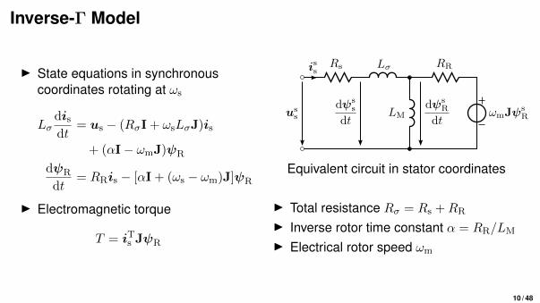
Inverse-Γ Model
I State equations in synchronouscoordinates rotating at ωs
Lσdisdt
= us − (RσI + ωsLσJ)is
+ (αI− ωmJ)ψR
dψR
dt= RRis − [αI + (ωs − ωm)J]ψR
I Electromagnetic torque
T = iTs JψR
dψss
dtωmJψs
R
RRissRs
uss LM
dψsR
dt
Lσ
Equivalent circuit in stator coordinates
I Total resistance Rσ = Rs +RR
I Inverse rotor time constant α = RR/LM
I Electrical rotor speed ωm
10 / 48
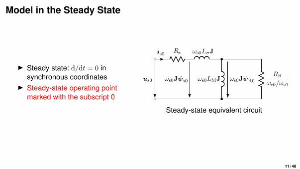
Model in the Steady State
I Steady state: d/dt = 0 insynchronous coordinates
I Steady-state operating pointmarked with the subscript 0
is0 ωs0LσJ
RR
ωr0/ωs0us0
Rs
ωs0LMJ ωs0JψR0ωs0Jψs0
Steady-state equivalent circuit
11 / 48
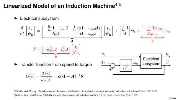
Linearized Model of an Induction Machine4,5
I Electrical subsystem
d
dt
[isψR
]=
[−RσLσ
I− ωs0J1Lσ
(αI− ωm0J)
RRI −αI− ωr0J
]︸ ︷︷ ︸
A
[isψR
]+
[ 1Lσ
I
0
]us +
[− 1Lσ
JψR0
JψR0
]︸ ︷︷ ︸
b
ωm
T =[−ψT
R0J iTs0J]︸ ︷︷ ︸
c
[isψR
]
I Transfer function from speed to torque
G(s) =T (s)
ωm(s)= c(sI−A)−1b
ωm
is
Electricalus
Tsubsystem1
sJm
TL
4Fallside and Wortley, “Steady-state oscillation and stabilisation of variable-frequency invertor-fed induction-motor drives,” Proc. IEE, 1969.5Nelson, Lipo, and Krause, “Stability analysis of a symmetrical induction machine,” IEEE Trans. Power App. Syst., 1969.
12 / 48
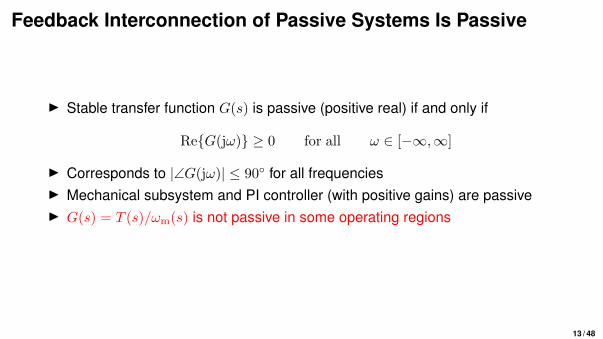
Feedback Interconnection of Passive Systems Is Passive
I Stable transfer function G(s) is passive (positive real) if and only if
Re{G(jω)} ≥ 0 for all ω ∈ [−∞,∞]
I Corresponds to |∠G(jω)| ≤ 90◦ for all frequenciesI Mechanical subsystem and PI controller (with positive gains) are passiveI G(s) = T (s)/ωm(s) is not passive in some operating regions
13 / 48
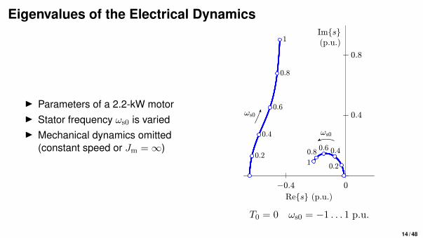
Eigenvalues of the Electrical Dynamics
I Parameters of a 2.2-kW motorI Stator frequency ωs0 is variedI Mechanical dynamics omitted
(constant speed or Jm =∞)
T0 = 0 ωs0 = −1 . . . 1 p.u.
14 / 48
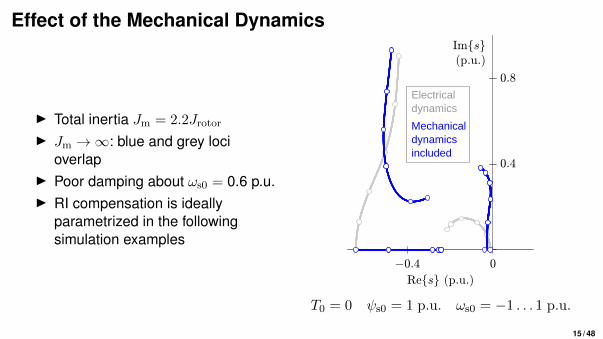
Effect of the Mechanical Dynamics
I Total inertia Jm = 2.2Jrotor
I Jm →∞: blue and grey locioverlap
I Poor damping about ωs0 = 0.6 p.u.I RI compensation is ideally
parametrized in the followingsimulation examples
Electrical dynamics
Mechanicaldynamicsincluded
T0 = 0 ψs0 = 1 p.u. ωs0 = −1 . . . 1 p.u.
15 / 48
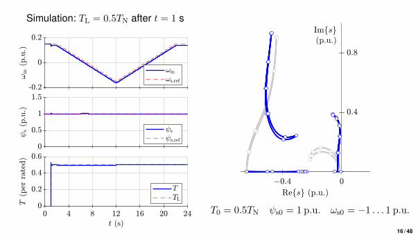
Simulation: TL = 0.5TN after t = 1 s
T0 = 0.5TN ψs0 = 1 p.u. ωs0 = −1 . . . 1 p.u.
16 / 48
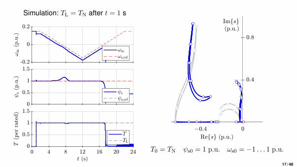
Simulation: TL = TN after t = 1 s
T0 = TN ψs0 = 1 p.u. ωs0 = −1 . . . 1 p.u.
17 / 48
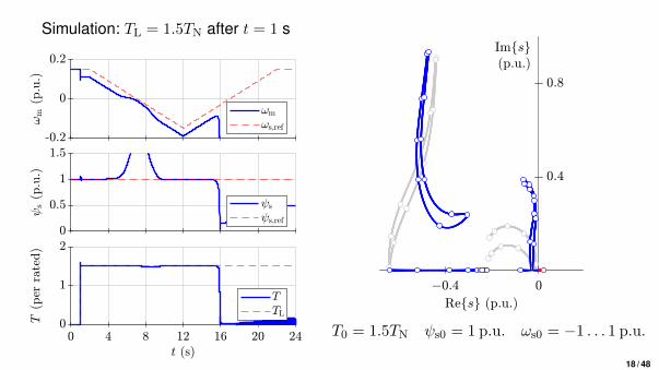
Simulation: TL = 1.5TN after t = 1 s
T0 = 1.5TN ψs0 = 1 p.u. ωs0 = −1 . . . 1 p.u.
18 / 48
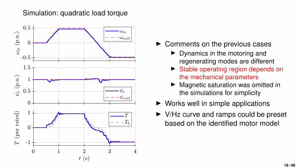
Simulation: quadratic load torque
I Comments on the previous casesI Dynamics in the motoring and
regenerating modes are differentI Stable operating region depends on
the mechanical parametersI Magnetic saturation was omitted in
the simulations for simplicityI Works well in simple applicationsI V/Hz curve and ramps could be preset
based on the identified motor model
19 / 48

Introduction
V/Hz Control
Observers
Sensorless Identification at Standstill
Sensorless, More or Less
20 / 48
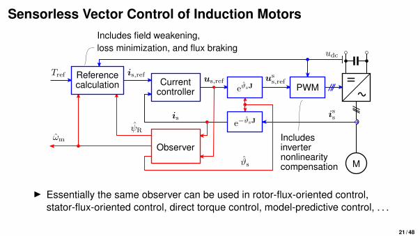
Sensorless Vector Control of Induction Motors
is,ref
ωm
isse−ϑsJ
eϑsJ
M
us,refCurrentcontroller
ψR
is
Observer
uss,ref
PWM
udc
Referencecalculation
Tref
inverternonlinearitycompensation
loss minimization, and flux brakingIncludes field weakening,
ϑs
Includes
I Essentially the same observer can be used in rotor-flux-oriented control,stator-flux-oriented control, direct torque control, model-predictive control, . . .
21 / 48
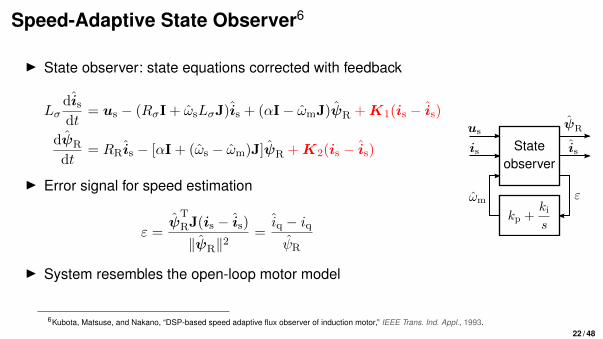
Speed-Adaptive State Observer6
I State observer: state equations corrected with feedback
Lσdisdt
= us − (RσI + ωsLσJ)is + (αI− ωmJ)ψR +K1(is − is)
dψR
dt= RRis − [αI + (ωs − ωm)J]ψR +K2(is − is)
I Error signal for speed estimation
ε =ψ
T
RJ(is − is)‖ψR‖2
=iq − iqψR
I System resembles the open-loop motor model
kp +kis
ωm
is
us
ε
ψR
observerState is
6Kubota, Matsuse, and Nakano, “DSP-based speed adaptive flux observer of induction motor,” IEEE Trans. Ind. Appl., 1993.22 / 48
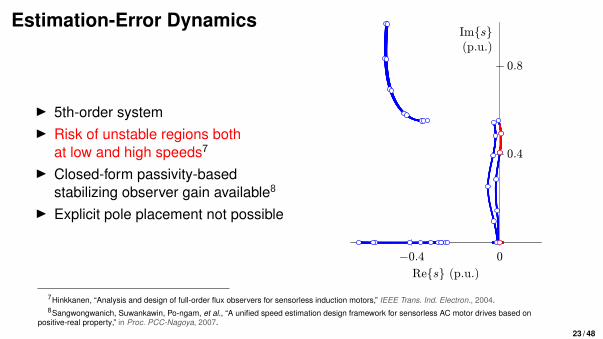
Estimation-Error Dynamics
I 5th-order systemI Risk of unstable regions both
at low and high speeds7
I Closed-form passivity-basedstabilizing observer gain available8
I Explicit pole placement not possible
7Hinkkanen, “Analysis and design of full-order flux observers for sensorless induction motors,” IEEE Trans. Ind. Electron., 2004.8Sangwongwanich, Suwankawin, Po-ngam, et al., “A unified speed estimation design framework for sensorless AC motor drives based on
positive-real property,” in Proc. PCC-Nagoya, 2007.23 / 48
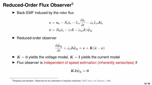
Reduced-Order Flux Observer9
I Back-EMF induced by the rotor flux
e = us −Rsis − Lσdisdt− ωsLσJis
e = RRis − (αI− ωmJ) ψR
I Reduced-order observer
dψR
dt+ ωsJψR = e+K(e− e)
I K = 0 yields the voltage model, K = I yields the current modelI Flux observer is independent of speed estimation (inherently sensorless) if
KJψR = 0
9Verghese and Sanders, “Observers for flux estimation in induction machines,” IEEE Trans. Ind. Electron., 1988.24 / 48
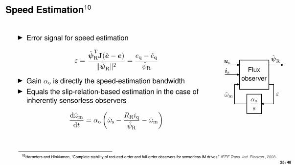
Speed Estimation10
I Error signal for speed estimation
ε =ψ
T
RJ(e− e)
‖ψR‖2=eq − eqψR
I Gain αo is directly the speed-estimation bandwidthI Equals the slip-relation-based estimation in the case of
inherently sensorless observers
dωm
dt= αo
(ωs −
RRiq
ψR
− ωm
) αo
s
ωm
is
us
ε
ψR
observerFlux
10Harnefors and Hinkkanen, “Complete stability of reduced-order and full-order observers for sensorless IM drives,” IEEE Trans. Ind. Electron., 2008.25 / 48
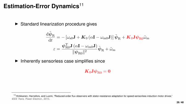
Estimation-Error Dynamics11
I Standard linearization procedure gives
dψR
dt= − [ωs0J +K0 (αI− ωm0J)] ψR +K0JψR0ωm
ε =ψT
R0J (αI− ωm0J)
‖ψR0‖2ψR + ωm
I Inherently sensorless case simplifies since
K0JψR0 = 0
11Hinkkanen, Harnefors, and Luomi, “Reduced-order flux observers with stator-resistance adaptation for speed-sensorless induction motor drives,”IEEE Trans. Power Electron., 2010.
26 / 48
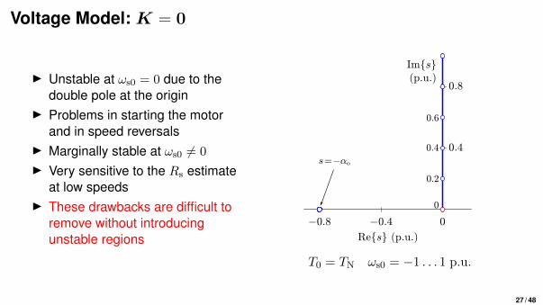
Voltage Model: K = 0
I Unstable at ωs0 = 0 due to thedouble pole at the origin
I Problems in starting the motorand in speed reversals
I Marginally stable at ωs0 6= 0
I Very sensitive to the Rs estimateat low speeds
I These drawbacks are difficult toremove without introducingunstable regions
T0 = TN ωs0 = −1 . . . 1 p.u.
27 / 48
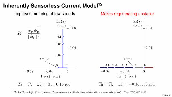
Inherently Sensorless Current Model12
Improves motoring at low speeds
K =ψRψ
T
R
‖ψR‖2
T0 = TN ωs0 = 0 . . . 0.15 p.u.
Makes regenerating unstable
T0 = TN ωs0 = −0.15 . . . 0 p.u.
12Ambrozic, Nedeljkovic, and Nastran, “Sensorless control of induction machine with parameter adaptation,” in Proc. IEEE ISIE, 1999.28 / 48
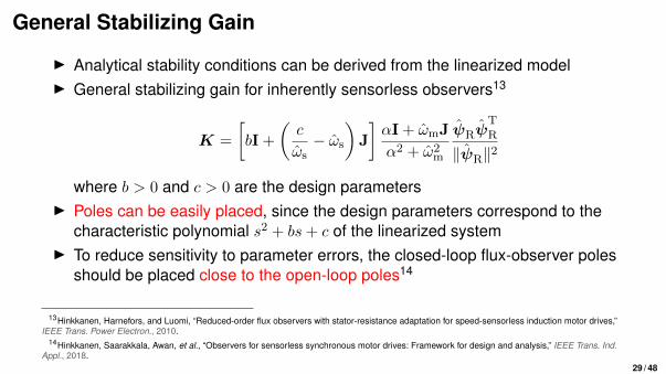
General Stabilizing Gain
I Analytical stability conditions can be derived from the linearized modelI General stabilizing gain for inherently sensorless observers13
K =
[bI +
(c
ωs− ωs
)J
]αI + ωmJ
α2 + ω2m
ψRψT
R
‖ψR‖2
where b > 0 and c > 0 are the design parametersI Poles can be easily placed, since the design parameters correspond to the
characteristic polynomial s2 + bs+ c of the linearized systemI To reduce sensitivity to parameter errors, the closed-loop flux-observer poles
should be placed close to the open-loop poles14
13Hinkkanen, Harnefors, and Luomi, “Reduced-order flux observers with stator-resistance adaptation for speed-sensorless induction motor drives,”IEEE Trans. Power Electron., 2010.
14Hinkkanen, Saarakkala, Awan, et al., “Observers for sensorless synchronous motor drives: Framework for design and analysis,” IEEE Trans. Ind.Appl., 2018.
29 / 48
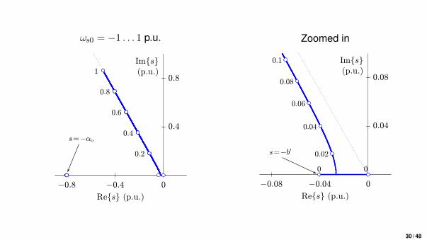
ωs0 = −1 . . . 1 p.u. Zoomed in
30 / 48
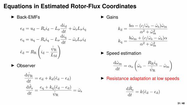
Equations in Estimated Rotor-Flux Coordinates
I Back-EMFs
ed = ud −Rsid − Lσdiddt
+ ωsLσiq
eq = uq −Rsiq − Lσdiqdt− ωsLσid
ed = RR
(id −
ψR
LM
)
I Observer
dψR
dt= ed + kd(ed − ed)
dϑsdt
=eq + kq(ed − ed)
ψR
= ωs
I Gains
kd =bα− (c/ωs − ωs)ωm
α2 + ω2m
kq =bωm + (c/ωs − ωs)α
α2 + ω2m
I Speed estimation
dωm
dt= αo
(ωs −
RRiq
ψR
− ωm
)I Resistance adaptation at low speeds
dRs
dt= k(ed − ed)
31 / 48
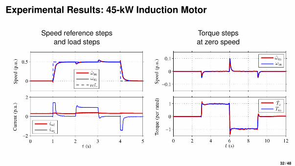
Experimental Results: 45-kW Induction Motor
Speed reference stepsand load steps
Torque stepsat zero speed
32 / 48
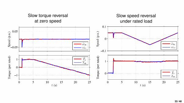
Slow torque reversalat zero speed
Slow speed reversalunder rated load
33 / 48

Introduction
V/Hz Control
Observers
Sensorless Identification at Standstill
Sensorless, More or Less
34 / 48
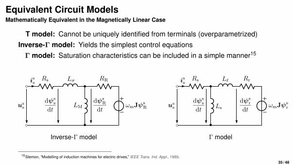
Equivalent Circuit ModelsMathematically Equivalent in the Magnetically Linear Case
T model: Cannot be uniquely identified from terminals (overparametrized)Inverse-Γ model: Yields the simplest control equations
Γ model: Saturation characteristics can be included in a simple manner15
dψss
dtωmJψs
r
RrissRs
uss
dψsr
dt
L`
Ls
dψss
dtωmJψs
R
RRissRs
uss LM
dψsR
dt
Lσ
Γ modelInverse-Γ model
15Slemon, “Modelling of induction machines for electric drives,” IEEE Trans. Ind. Appl., 1989.35 / 48
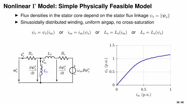
Nonlinear Γ Model: Simple Physically Feasible ModelI Flux densities in the stator core depend on the stator flux linkage ψs = ‖ψs‖I Sinusoidally distributed winding, uniform airgap, no cross-saturation
ψs = ψs(im) or im = im(ψs) or Ls = Ls(im) or Ls = Ls(ψs)
dψss
dtωmJψs
r
RrissRs
uss
dψsr
dt
L`
Ls
ism
36 / 48
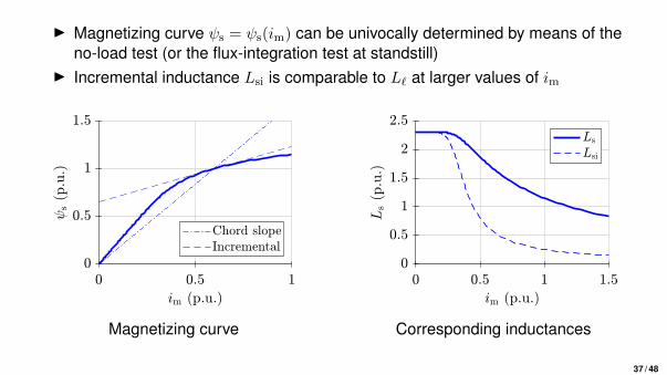
I Magnetizing curve ψs = ψs(im) can be univocally determined by means of theno-load test (or the flux-integration test at standstill)
I Incremental inductance Lsi is comparable to L` at larger values of im
Magnetizing curve Corresponding inductances
37 / 48
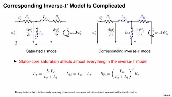
Corresponding Inverse-Γ Model Is Complicated
dψss
dtωmJψs
r
RrissRs
uss
dψsr
dt
L`
Ls
dψss
dtωmJψs
R
RRissRs
uss LM
dψsR
dt
Lσ
Saturated Γ model Corresponding inverse-Γ model
I Stator-core saturation affects almost everything in the inverse-Γ model
Lσ =LsL`Ls + L`
LM = Ls − Lσ RR =
(Ls
Ls + L`
)2
Rr
The equivalence holds in the steady state only, since some incremental inductance terms were omitted the transformation.38 / 48
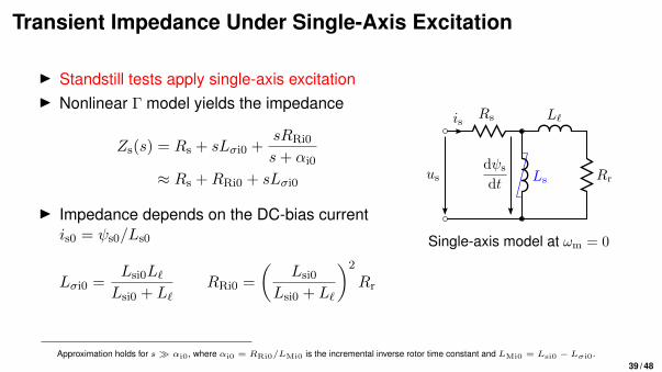
Transient Impedance Under Single-Axis Excitation
I Standstill tests apply single-axis excitationI Nonlinear Γ model yields the impedance
Zs(s) = Rs + sLσi0 +sRRi0
s+ αi0
≈ Rs +RRi0 + sLσi0
I Impedance depends on the DC-bias currentis0 = ψs0/Ls0
Lσi0 =Lsi0L`Lsi0 + L`
RRi0 =
(Lsi0
Lsi0 + L`
)2
Rr
dψs
dtRr
is Rs
us
L`
Ls
Single-axis model at ωm = 0
Approximation holds for s � αi0, where αi0 = RRi0/LMi0 is the incremental inverse rotor time constant and LMi0 = Lsi0 − Lσi0.39 / 48
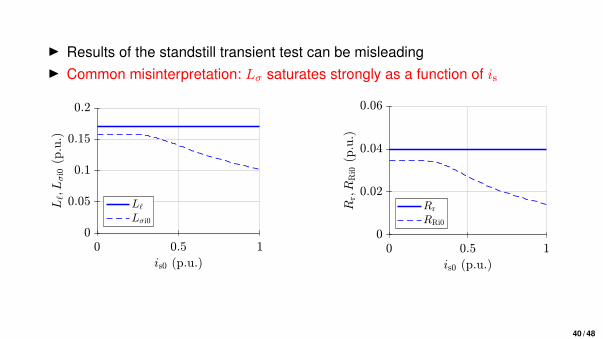
I Results of the standstill transient test can be misleadingI Common misinterpretation: Lσ saturates strongly as a function of is
40 / 48
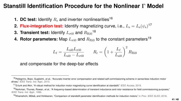
Stanstill Identification Procedure for the Nonlinear Γ Model
1. DC test: Identify Rs and inverter nonlinearities16
2. Flux-integration test: Identify magnetizing curve, i.e., Ls = Ls(ψs)17
3. Transient test: Identify Lσi0 and RRi018
4. Rotor parameters: Map Lσi0 and RRi0 to the constant parameters19
L` =Lsi0Lσi0Lsi0 − Lσi0
Rr =
(1 +
L`Lsi0
)2
RRi0
and compensate for the deep-bar effects
16Pellegrino, Bojoi, Guglielmi, et al., “Accurate inverter error compensation and related self-commissioning scheme in sensorless induction motordrives,” IEEE Trans. Ind. Appl., 2010.
17Erturk and Akin, “A robust method for induction motor magnetizing curve identification at standstill,” IEEE Access, 2019.18Kerkman, Thunes, Rowan, et al., “A frequency-based determination of transient inductance and rotor resistance for field commissioning purposes,”
IEEE Trans. Ind. Appl., 1996.19Khamehchi, Molsa, and Hinkkanen, “Comparison of standstill parameter identification methods for induction motors,” in Proc. IEEE SLED, 2018.
41 / 48
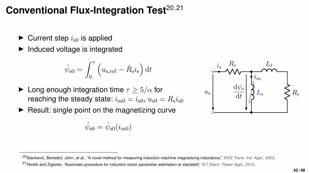
Conventional Flux-Integration Test20,21
I Current step is0 is appliedI Induced voltage is integrated
ψs0 =
∫ τ
0
(us,ref − Rsis
)dt
I Long enough integration time τ ≥ 5/α forreaching the steady state: im0 = is0, us0 = Rsis0
I Result: single point on the magnetizing curve
ψs0 = ψs0(im0)
dψs
dtRr
is Rs
us
L`
Ls
im
20Stankovic, Benedict, John, et al., “A novel method for measuring induction machine magnetizing inductance,” IEEE Trans. Ind. Appl., 2003.21Peretti and Zigliotto, “Automatic procedure for induction motor parameter estimation at standstill,” IET Electr. Power Appl., 2012.
42 / 48
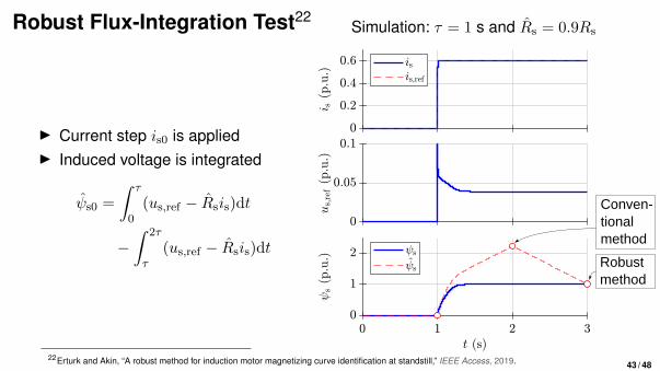
Robust Flux-Integration Test22
I Current step is0 is appliedI Induced voltage is integrated
ψs0 =
∫ τ
0(us,ref − Rsis)dt
−∫ 2τ
τ(us,ref − Rsis)dt
Simulation: τ = 1 s and Rs = 0.9Rs
Robustmethod
Conven-tionalmethod
22Erturk and Akin, “A robust method for induction motor magnetizing curve identification at standstill,” IEEE Access, 2019. 43 / 48
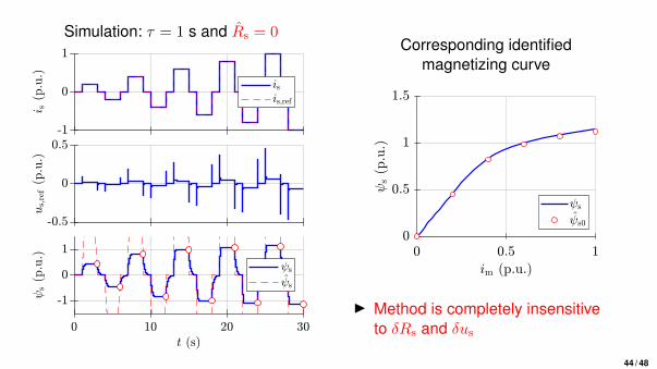
Simulation: τ = 1 s and Rs = 0Corresponding identified
magnetizing curve
I Method is completely insensitiveto δRs and δus
44 / 48

Introduction
V/Hz Control
Observers
Sensorless Identification at Standstill
Sensorless, More or Less
45 / 48
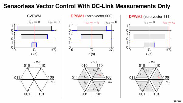
Sensorless Vector Control With DC-Link Measurements Only
Ts
01
0
00 2Ts
1
1
t (s)Ts
01
0
00 2Ts
1
1
t (s)Ts
01
0
00 2Ts
1
1
t (s)
SVPWM DPWM1 (zero vector 000) DPWM2 (zero vector 111)idc = iaidc = 0 idc = −icidc = 0 idc = 0 idc = 0
−ia
100
110010
011
001 101
uα
uβ
−ia
−ib−ib
−ic
−ic
ia
100
110010
011
001 101
uα
uβ
ia
ibib
icic
100
110010
011
001 101
uα
uβ
46 / 48
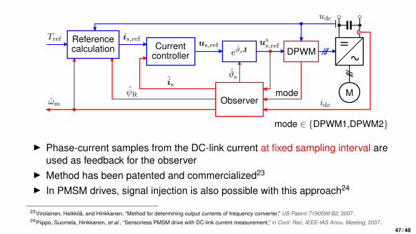
is,ref
ωm
eϑsJus,refCurrent
controller
ψR
is
Observer
uss,ref
DPWM
udc
Referencecalculation
Tref
ϑs
Midc
mode
mode ∈ {DPWM1,DPWM2}
I Phase-current samples from the DC-link current at fixed sampling interval areused as feedback for the observer
I Method has been patented and commercialized23
I In PMSM drives, signal injection is also possible with this approach24
23Virolainen, Heikkila, and Hinkkanen, “Method for determining output currents of frequency converter,” US Patent 7190599 B2, 2007.24Piippo, Suomela, Hinkkanen, et al., “Sensorless PMSM drive with DC-link current measurement,” in Conf. Rec. IEEE-IAS Annu. Meeting, 2007.
47 / 48
ConclusionsI V/Hz control is plug-and-play due to its simplicity
I Unstable regions due to interaction of the electrical and mechanical dynamicsI Works well in simple applications (pumps and fans)
I Plug-and-play sensorless vector control enables a wider range of applicationsI Requires advanced observer and self-commissioning algorithmsI Can stabilize the system completely (except at zero stator frequency under load)I Temperature-dependent Rs can be tracked on-line, if the magnetic model knownI Magnetic model can be identified at standstill
I PMSMs and SyRMs were not covered hereI Similar problems (and similar solutions)I In addition, signal injection can be used to stabilize the lowest speeds
I Role of IoT and machine learning in the future?
48 / 48