Embed Size (px)
Citation preview

Sensor Fusion Techniques
Dr Robert Harle
Part II Mobile and Sensor Systems
Lent 2017/18

Measurements are Noisy A sensor measures some quantity with some accuracy.
Whatever we do, noise will creep in We therefore need to fuse multiple measurements to
get a robust idea of what's happening
Fusionalgorithm
State estimate(and error)
Multiple measurements from same sensor
[Domain-specifc constraints]
Multiple measurements from diferent sensors

Algorithms There are many fusion techniques and algorithms We will look at the two extremes: a very fast, very common
algorithm that is limited in what it works with, and a general-purpose and fexible but more computationally demanding algorithm
Both are based on bayesian probability We will use location tracking to illustrate the techniques
because the problem is easy to relate to. But everything is general.

Simple Tracking ExampleConsider a series of positions that come in a few seconds apart for a pedestrian. They will probably look rather unrealistic for a walking route:

Simple Tracking ExampleBut if we consider noise and error in the measurements we see that the data supports a more realistic hypothesis of straight line walking:

Probabilistic ApproachSo what we want to do is to estimate our current state while incorporating knowledge of recent measurements and all of the associated errors. To do this we will use probability:
State at time t(e.g. position)
Belief (probability)
Measurements(e.g. from positioning system)

Filters and Smoothers
This is known as a flter because it estimates the current state based on current and past measurements (only)
Sometimes you know the ‘future’ e.g. you may have logged data for postprocessing rather than live processing
In that case you have a smoother
Recursive Bayesian Filters Apply a Markov model (next state depends only on last) to
recursively build up our probabilities
This is the propagation or prediction step We update the probabilities based on some model (e.g.
constant velocity) → prior distribution
PriorPropagation (motion)model
Evaluate overall previous states

Recursive Bayesian Filters Apply Bayes' theorem to incorporate measurements
This is the correction or update step We correct the probabilities on a measurement →
posterior distribution
Posterior MeasurementmodelNorm
factor
Prior

Implementation
There are broadly two classes of techniques to implement these “flters”1) Model all the probability distributions using mathematical
models. This keeps everything continuous. But it's not always easy to do this (the distributions get complex). E.g. Use Gaussians everywhere → “Kalman Filter”
2) Represent arbitrary distributions by sampling them. Nice and general but much more work involved.
Propagation/predict
Correction/update

The Kalman Filter

Simple example
Motion along a straight path State vector [x, dx/dt]T
dx/dt
x

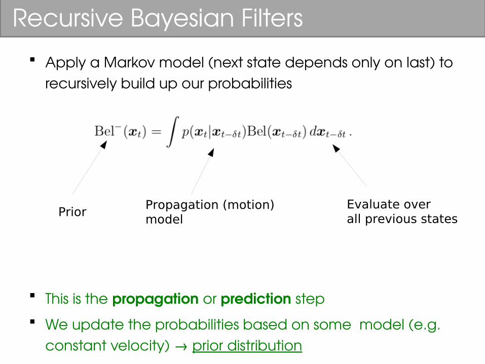
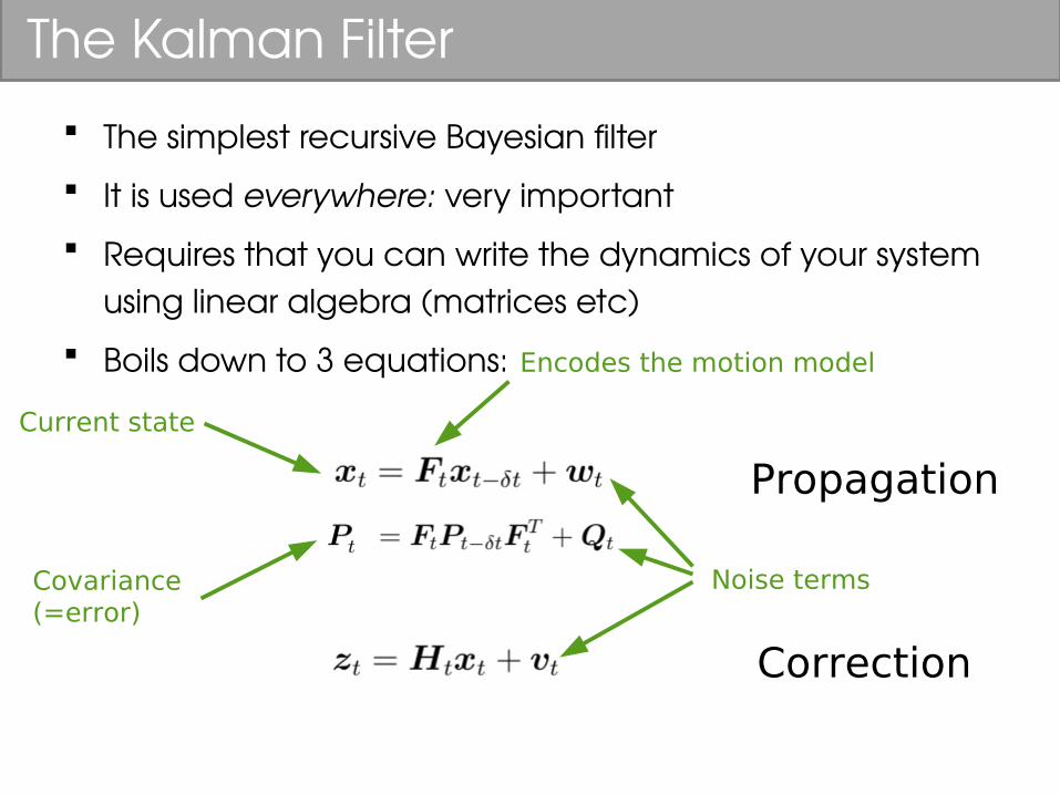
The Kalman Filter The simplest recursive Bayesian flter It is used everywhere: very important Requires that you can write the dynamics of your system
using linear algebra (matrices etc) Boils down to 3 equations:
Propagation
Correction
Current state

The Kalman Filter The simplest recursive Bayesian flter It is used everywhere: very important Requires that you can write the dynamics of your system
using linear algebra (matrices etc) Boils down to 3 equations:
Propagation
Correction
Current state
Encodes the motion model

Simple example
Motion model (constant velocity)
F = 1 dt0 1

The Kalman Filter The simplest recursive Bayesian flter It is used everywhere: very important Requires that you can write the dynamics of your system
using linear algebra (matrices etc) Boils down to 3 equations:
Propagation
Correction
Current state
Encodes the motion model
Noise terms
The Kalman Filter The simplest recursive Bayesian flter It is used everywhere: very important Requires that you can write the dynamics of your system
using linear algebra (matrices etc) Boils down to 3 equations:
Propagation
Correction
Covariance(=error)
Current state
Encodes the motion model
Noise terms
Measurement model (how the measurement relates to the state)

Simple example
Measurement model (just measure position directly)
H = (1 0)

The Nitty Gritty
(Thanks to wikipedia. No, you aren't expected to learn these)

Key to the Kalman Filter
Initially we have some position estimate that is associated with a normal distribution

Key to the Kalman Filter
We propagate the state, meaning we use the motion model to move it forward. Since we had no actual input, we increase the error (→ Gaussian gets shorter and fatter)

Key to the Kalman Filter
We repeat the propagation but then a measurement comes in. This is associated with another Gaussian, although thinner because it's an OK estimate

Key to the Kalman Filter
The beauty of a Gaussian is that when you multiply two together you get another Gaussian. Thus we always fnish a cycle with a new Gaussian estimate → we can represent it using just two parameters, making it amenable to linear algebra

So...
[ An example ]

A more complex example Consider the Inertial GPS systems you fnd in vehicles They need to estimate where the car is at all times
between GPS measurements We compute position by concatenating a series of
displacements and headings (dead reckoning) We use inertial sensors to estimate the displacements
(wheel encoders) and headings (gyroscopes) since the last state estimate
t=1t=0 t=2
t=2

Inertial Nav We integrate the gyroscope signal to estimate the heading
change (note the motion model uses the inertial inputs) But gyros are subject to bias errors (a bias is a bogus ofset
reported when it's not rotating) and we often see erroneous bending:
True(unobservable)
INS bias bends heading
Estimate

Inertial Nav When a GPS measurement comes in we can fx
things
GPS
True(unobservable)
INS
GPS correction

Inertial Nav But if we just correct position, it goes wrong again
GPS
True(unobservable)
INS
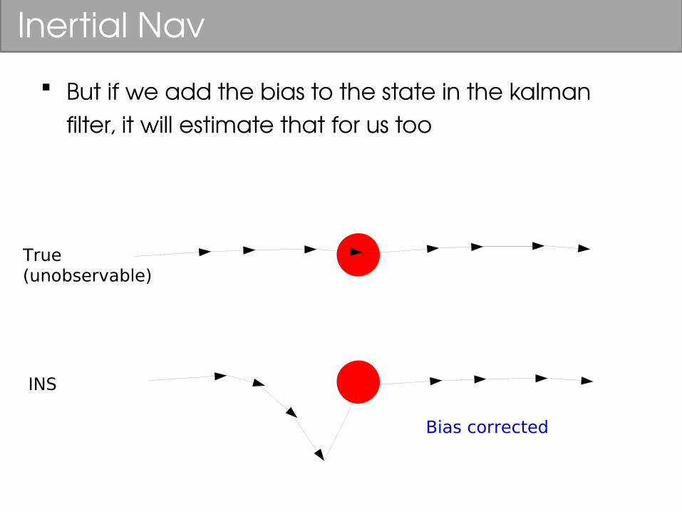
Inertial Nav But if we add the bias to the state in the kalman
flter, it will estimate that for us too
True(unobservable)
INS
Bias corrected

KF Limitations
What if those probability distributions don't lend themselves to being normal?
Our example will be constraining movement to be on a building foorplan. How could you build a motion model matrix that incorporated a foorplan??!
Propagation
Correction

The Particle Filter

Our Example Imagine tracking someone around a building using
the sensors on their phone and a foorplan We now estimate step events where a step has a
length associated with it and a direction.
Easy to spot steps when looking at the accelerometer
Integrating the gyro gives direction change as before

Particle Filters for Location
Encode state in particles. Each particle is just an individual hypothesis about the position and orientation of the user
Each particle has an assigned probability
Particles are updated by: Propagation/Predict Correct [Resample]
P=0.1
P=0.21
P=0.05
P=0.01
P=0.05
P=0.2

PF: Propagate
Each particle is moved by the measured step length and direction
Plus some additive noise that represents the imperfect measurement
θ+noise
L+noise
N

PF: Propagate
Each particle is moved by the measured step length and direction
Plus some additive noise that represents the imperfect measurement
θ+noise
L+noise
N

PF: Propagate
Each particle is moved by the measured step length and direction
Plus some additive noise that represents the imperfect measurement
θ+noise
L+noise
N

Cloud Spread With each step, the particle cloud
spreads naturally due to the noise we add
This is good: it represents that our drift (→ uncertainty) is growing (c.f. the Gaussian growing fatter with each step of the KF)

PF: Correct Given a measurement we can reassign the
particle probabilities If we had an absolute position (maybe
a GPS fx) we could weight to that position
0.2
0.2
0.2
0.2
0.2

GPS
PF: Correct Given a measurement we can reassign the
particle probabilities If we had an absolute position (maybe
a GPS fx) we could weight to that position
0.2
0.2
0.2
0.2
0.2

GPS
PF: Correct Given a measurement we can reassign the
particle probabilities If we had an absolute position (maybe
a GPS fx) we could weight to that position
0.2
0.2
0.2
0.2
0.2
0.3
0.1
0.1
0.1
0.4

PF: Correct Constraints can be included as pseudo-
measurements For walls we can simply set p=0 if the particle
crossed a wall and leave it alone otherwise
Pn+1
=0
Pn+1
=1
Pn=1
Pn=1

PF: Resample Want to get rid of p=0 particles but still need some
particles! We resample: generate a new particle set by
sampling the old one in proportion to the particle weights
P=0 → won't go any further P=1 → may be reproduced (multiple times) if chosen
at random

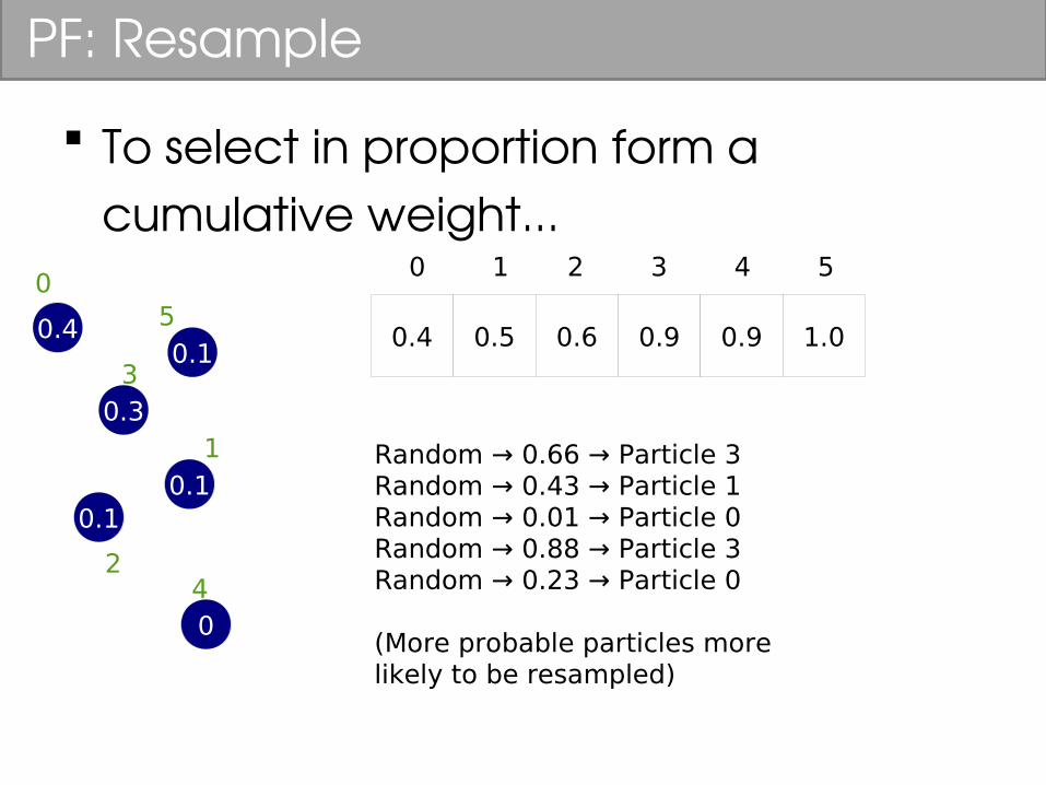
PF: Resample
To select in proportion form a cumulative weight...
Particle number
CumulativeWeight (CW)
0.3
0.1
0.1
0.1
0.4

PF: Resample
To select in proportion form a cumulative weight...
Particle number
CumulativeWeight (CW)
0.3
0.1
0.1
0.1
0.4
Random no
P3
Random no
P5
PF: Resample
To select in proportion form a cumulative weight...
0.3
0.1
0.1
0.1
0.4
05
3
1
240
0.4 0.5 0.6 0.9 0.9 1.0
0 1 2 3 4 5
Random → 0.66 → Particle 3Random → 0.43 → Particle 1Random → 0.01 → Particle 0Random → 0.88 → Particle 3Random → 0.23 → Particle 0
(More probable particles more likely to be resampled)

A Note on Performance
Update and correct steps are nicely parallelisable
But forming the cumulative weight for resampling is fundamentally sequential...

Works well...
Initially we have no knowledge of the user's position Lots of particles Localisation
Phase

Symmetry Problem

Works well... Eventually we fgure out
where they are and the problem becomes easier Fewer particles
needed Tracking Phase
We got ~ 0.75m accuracy 95% of the time with a sensor on the shoe

In General Particle flters are easy to implement and highly
fexible But:
Every particle you add costs you in terms of computation
The results are not deterministic Too few particles gives bad/failed results, while too
many wastes precious CPU cycles


![Multi-Sensor Fusion - Store & Retrieve Data Anywhere€¦ · Origin Multi-sensor fusion is also known as multi-sensor data fusion [1, 2], which is an emerging technology originally](https://img.pdfslide.us/doc/110x75/5b6da87a7f8b9aa32b8d015c/multi-sensor-fusion-store-retrieve-data-anywhere-origin-multi-sensor-fusion.jpg)


![[FRC 2012] Sensor Fusion Tutorial](https://img.pdfslide.us/doc/110x75/577cdfcd1a28ab9e78b20184/frc-2012-sensor-fusion-tutorial.jpg)