Sensor and gateway location optimization in body sensor networks

Mari Carmen Domingo

� Springer Science+Business Media New York 2014

Abstract In body sensor networks (BSNs), energy-con-

strained sensors monitor the vital signs of human beings in

healthcare applications. Energy consumption is a funda-

mental issue, since BSNs must operate properly and

autonomously for long period of time without battery

recharge or replacement. In addition, the human exposure

to electromagnetic radiation must be limited. For all these

reasons, the energy consumption in BSNs should be min-

imized. In this paper, sensor and gateway location opti-

mization for BSNs has been analyzed. A mathematical

model has been proposed to minimize the energy con-

sumption of the BSN and the heating effects on human

tissues. We distinguish between ‘in-body’ and ‘on-body’

sensors depending on their location inside or outside the

human body, respectively. The theoretical analysis and the

numerical results reveal that in in-BSNs the energy con-

sumption can be significantly reduced when the optimal

positions of the gateway or the sensors are computed.

However, in on-BSNs the energy consumption is not

affected by the devices’ location. With power control the

interferences are minimized and the human exposure to

electromagnetic radiation is reduced.

Keywords Body sensor networks � Location

optimization � Power control � Energy consumption

1 Introduction

Body sensor networks (BSNs) consist on smart miniatur-

ized devices that can be worn or implanted [1]. They allow

the monitoring of health information with the help of

sensors using low power technology [2].

The energy consumption in BSNs should be decreased

due to the following reasons. First, in BSNs, energy-con-

strained sensors monitor the vital signs of human beings in

healthcare applications. Furthermore, BSNs should be able

to operate without battery recharge or replacement during a

long time [3]. In addition, during communication the devices

emit Radiofrequency (RF) fields, which generate heat. This

heat is absorbed by the surrounding tissue and increases the

body temperature [4]. This temperature rise should be lim-

ited, since the body tissues are sensitive to temperature

increase and may be damaged. The Specific Absorption Rate

(SAR) is a measure of the power absorbed by the tissue in

the body. This parameter should be minimized, since BSNs

operate inside, on or in close proximity to the human body.

BAN devices shall comply with international or local SAR

regulations. For instance, the limit for exposure in the head

is a SAR level of 1.6 W/kg in 1 g for US and 2 W/kg in

10 g for Europe. Therefore, the transmission power limits

are lower than 1.6 mW for US and lower than 20 mW for

Europe [5]. The transmission power is related to the dis-

tance-dependent energy consumption [6] (see Eq. (1) in

Sect. 4.1). Ideally, the energy consumption is minimized

when the distance between the source and destination nodes

is minimal and this distance depends on the node location.

Consequently, the optimization of node locations can min-

imize the energy consumption.

In this paper, location optimization for BSNs has been

studied via a theoretical analysis and numerical evalua-

tions. Two different cases have been proposed to find the

M. C. Domingo (&)

Electrical Engineering Department, UPC-Barcelona

Tech University, Esteve Terrades, 7, 08860 Castelldefels,

Barcelona, Spain

e-mail: cdomingo@entel.upc.edu

123

Wireless Netw

DOI 10.1007/s11276-014-0745-7

optimal location for (1) the gateway or (2) the body sen-

sors, respectively. A mathematical model has been devel-

oped for each case to find the best placement. The major

objective of the proposed mathematical model is to mini-

mize the energy consumption of the BSN and the heating

effects on human tissues. To the best of our knowledge,

this is the first paper that analyzes where the optimal

location is of the gateway or the body sensors to minimize

the energy consumption.

It has been shown that the energy consumption of in-

BSNs is significantly decreased when the gateway or the

sensors are located at their optimal positions. On the con-

trary, the energy consumption of on-BSNs does not depend

on the devices’ location.

The paper is structured as follows. In Sect. 2, we discuss

the related work on node location in BSNs. In Sect. 3, we

analyze our system model. In Sect. 4, we state the location

optimization problems and propose nonlinear programming

(NLP) formulations. In Sect. 5, we present our numerical

results. Finally, we draw the conclusions in Sect. 6.

2 Related work

In this paper, we focus on node location in BSNs. The

sensor signals depend significantly on the placement of the

sensors on/in the human body [7]. In [8], changes in node

orientation, node placement, body position and environ-

mental factors are analyzed to determine their influence on

BSN communication. The authors conclude that connec-

tivity is affected by node location as well as body position.

Other experiments carried out in [9] with seven nodes

located on different parts of the body, two scenarios

(anechoic camber and meeting room) and two positions

(sitting and standing) show that the human body clearly

modifies communication properties, introducing attenua-

tions of up to 26 dB. In [10], the position of the gateway

(transmitter) is selected between three different positions:

stomach, right wrist, left wrist. The positions of the sensors

(receivers) are selected according to their potential medical

applications at different body parts. It is shown that the

path loss varies depending on the transmitter and receiver

locations. In our paper, we support these conclusions [8, 9,

10] with a further study to determine the optimal locations

of the sensor nodes and the gateway in a BSN.

The optimal sensor location for a BSN is an important

topic. Sensor location information is helpful for activity

recognition [7]. The misplacement of sensors results in

false physical activity recording and invalidates the mon-

itoring [11]. In [12], the authors study which is the ideal

location for accelerometers according to a given group of

activities and how to discriminate between these activities.

In [13], several sensor positions to detect stereotypical self-

stimulatory behavioral patterns of children with Autism

Spectrum Disorder (ASD) are investigated. The purpose of

this study is to find optimal locations for sensor placement

for self-stimulatory behavior detection. This way, it was

possible to detect rocking events and body motions when

the sensor system was worn on the back of autistic patients.

The detection of flapping by locating sensors at the wrist

was more accurate than if these sensors were located on the

back; however, the number of false positives was increased

as well due to hand movements. In [14], it is shown that the

heart rate signal measured around the ear has a similar

magnitude than the one measured at the fingertip. In [15], it

is explained after analyzing the kinematics that the chest is

the optimal sensor placement to predict a fall event before

it happens (pre-impact recognition) or after it has already

happened (post-fall detection). In [16], the authors state

that the best location of a sensor is not always the place

where its symptoms appear. For instance, head-worn sen-

sors can detect gait features better than sensors located on

the legs, since the head remains relatively stable compared

to the trunk when somebody moves and its direction is

more representative when the individual is moving. Con-

sequently, further studies are needed to determine optimal

areas on the body where sensors should be placed. In the

second part of our paper, the optimal locations for some

sensors are found assuming the body regions with the

highest symptom detection rates for particular conditions

are provided.

3 System model analysis

Our network architecture is shown in Fig. 1. A BSN is used

for healthcare monitoring. The physiological states of the

Fig. 1 Network architecture

Wireless Netw

123

person are being sensed, sampled and processed by specific

implant and body surface sensors. Implant sensors are

located inside the human body, whereas body surface

sensors are placed at the human skin or at most 2 cm away.

In this architecture, each implant or body surface sensor si

monitors the physiological states of a person and transmits

this information towards a gateway located at the body

surface using single-hop communication. The sensors

communicate with the gateway using ultra-wideband

(UWB) or the standard 802.15.6. Afterwards, the gateway

transmits this data to a monitoring station using Bluetooth

or Zigbee. The monitoring station is connected to a Wide

Area Network (WAN) for remote data access. Monitoring

stations can access the radio channel using different

transmission media including Wireless Local Area net-

works (WLANs), Worldwide Interoperability for Micro-

wave Access (WiMax), General Packet Radio Service

(GPRS), and Wideband Code Division Multiple Access

(WCDMA).

4 Problem formulation and optimization model

We consider the network topology shown in Fig. 1. We

assume that the BSN is set on a person standing with arms

and legs together and stuck to the body.

We assume that certain sensor nodes should be placed at

fixed positions on (on-body communication) or inside the

human body (in-body communication), which are deter-

mined by the functionality of the sensors. For example, the

patch-type ECG sensors should be placed on the chest

along the central axis of the heart, since they are used to

measure the electrical activity of this organ. Their positions

can only be slightly altered inside this area.

On the contrary, other nodes don’t have stringent

placement restrictions. Their positions can be selected from

a range of possible locations. As an example, motion

sensors can be placed at different locations (ankle, hip)

depending on the data to be measured [17] and temperature

sensors [4] can be placed almost anywhere.

We consider the following cases, which will be solved

differently:

Case

1

The positions of the sensors si are fixed depending

on their functionality. The optimal location for the

gateway g needs to be found

Case

2

The position of the gateway g is fixed. The

positions of the sensors si can be selected between

certain ranges of possible locations. The optimal

positions for the sensors need to be found

One of the challenges of our proposal is that some

standards for the measurement of the human body are

required to locate the sensors and the gateway properly.

Leonardo da Vinci used human body measurements when

he was sketching a human figure entitled ‘Vitruvian Man’.

This drawing is based on a model of ideal proportions

established by the ancient Roman Vitruvius. The list of

standard bodily proportions used is the following (see

Fig. 2) [18]:

• The average human is seven heads tall.

• The width from shoulder to shoulder is three heads

width.

• The distance from the hip to the toes is four heads.

• The distance from the top of the head to the bottom of

the chest is 2 heads.

• The distance from the wrist to the end of the

outstretched fingers of the hand is 1 head.

• The length from top to bottom of the buttocks is 1 head.

• The distance from the elbow to the end of outstretched

fingers is 2 heads.

These human body dimensions vary according to the

sex, age, race, socio-economical level, etc. Future work

includes conducting several experiments to analyze the

performance of our system model using a human body/

phantom.

4.1 Case 1

Next, case 1 will be solved. The positions of the sensor

nodes si are fixed and depend on their functionality. The

optimal location for the gateway g needs to be found. We

formulate this problem as a NLP.

Fig. 2 Standards for the measurement of the human body

Wireless Netw

123

We introduce the following notation:

• S = {s1, s2, …, sN} is a finite set of body sensors with

N = |S|. They are traffic sources.

• D = {d1, d2, …, dN} is the array, whose i-th element

contains the value of the distance between the node si

and the gateway g.

• (S, D) is the representation of the BSN.

• P = {(si, g): si [ S, g [ G} is the set of source-gateway

connections.

• ui = (xi, yi, zi) is the location of the node si.

• v = (xg, yg, zg) is the location of the gateway g.

• X is the set of possible locations for the sensors or for

the gateway in a human body.

• BN is the noise bandwidth.

• vTX is the data rate.

• Pn is the noise power in dBm.

• PT is the transmission power in dBm.

• PL is the path loss.

• PL1-MAX is the maximum path loss threshold for in-

body communication.

• PL2-MIN is the minimum path loss threshold for on-body

communication.

• PL2-MAX is the maximum path loss threshold for on-

body communication.

• h is the head length.

The energy consumption per packet for node si or

energy cost can be computed as [19]:

ECOMi ðDÞ ¼ EampðnÞ � dn

i þ ETX�elec þ ERX�elec

� �� q ð1Þ

where Eamp refers to the energy consumed by the transmit

amplifier, di is the distance between the sensor node si and

the gateway g, n represents the path loss coefficient and q is

the packet size. ETX-elec refers to the energy per bit needed

by transmitter electronics and digital processing and ERX-

elec refers to the energy per bit needed by the receiver

electronics. Every term is multiplied by the average packet

size q.

The problem can be formulated as follows:

P1: Location Optimization Problem

Given : ui 2 X;BN ; vTX;Pn;PT

Find : v 2 X ; di 2 D

Min :P

i2S

ECOMi Dð Þ � Ni

� �

Subject to:

Ni ¼ 1� PERið Þ�1 ð2Þ

PERi ¼ 1� 1� BERið Þq ð3Þ

BERooki ¼ 1

2erfc

ffiffiffiffiffiffiffiffiffiffiffiffiffiffiffiffiffi1

4

Eb

N0

� �

i

s !

ð4Þ

or

BERBPSKi ¼ 1

2erfc

ffiffiffiffiffiffiffiffiffiffiffiffiffiffiEb

N0

� �

i

s !

ð5Þ

Eb

N0

� �

i

¼ wi

BN

vTX

ð6Þ

wiðdiÞ ¼ PRðdiÞ � Pn ð7ÞPR dið Þ ¼ PT � PL dið Þ ð8Þ

In-body communication

PL dið Þ�PL1�MAX ð9Þ

or

On-body communication (line-of-sight (LOS))

PL2�MIN �PL dið Þ�PL2�MAX ð10Þdi ¼ ui � vk k; 8di 2 D ð11Þ�0:5h� xg� 0:5h and 3:2h� yg� 3:5h and zg ¼ 0 ð12Þ

or

�1:5h� xg� 1:5h and 0:5h� yg� 2:5h and zg ¼ 0 ð13Þ

or

�h� xg� h and � 3:2h� yg� � 0:5h and zg ¼ 0 ð14Þ

or

h� xg� 1:5h and � h� yg� 0:5h and zg ¼ 0 ð15Þ

or

�1:5h� xg� � h and � h� yg� 0:5h and zg ¼ 0 ð16Þ

or

�h� xg�h and � 3:5h� yg� � 3:2h and zg ¼4h

5ð17Þ

or

�0:5h� xg� 0:5h and 3:2h� yg� 3:5h and zg ¼ �4h

5

ð18Þ

or

�1:5h� xg�1:5h and 0:5h� yg�2:5h and zg ¼�h ð19Þ

or

�h� xg� h and � 3:5h� yg� � 0:5h and zg ¼ �h

2

ð20Þ

or

h� xg� 1:5h and � h� yg� 0:5h and zg ¼ �h

5ð21Þ

Wireless Netw

123

or

�1:5h� xg� � h and � h� yg� 0:5h and zg ¼ �h

5

ð22Þ

The objective function of problem P1 aims at finding the

best location for the gateway g that minimizes the energy

cost of the overall BSN for successful packet reception. It

is worth noting that constraints (7, 8, 9 and 10) as well as

the energy cost EiCOM(D) in (1) depend all on di. As the

objective function in our optimization is non-linear and

depends on di’s as well as on v = (xg, yg, zg), the problem

P1 is a non-linear optimization problem.

Constraint (2) determines the average number of packet

transmissions for successful decoding at the gateway. In

constraint (3), the Packet Error Rate (PER) for a packet

transmission of q bits using the CRC block detection

mechanism is given. Two modulation schemes have been

selected for the analysis: On–Off Keying (OOK) due to its

low-power operation and Binary Phase Shift Keying (BPSK)

due to its BER improvement [20]. The BER for OOK and

BPSK modulations over an Additive White Gaussian Noise

(AWGN) channel are expressed by constraints (4 and 5),

respectively. The ratio (Eb/N0)i of the average energy per

information bit to the noise power spectral density at the

receiver input is given by constraint (6). The signal to noise

ratio (SNR) Wi at the receiver is given by constraint (7). The

received power PR at a receiver at distance di from the

transmitter is given by constraint (8).

Constraints (9 and 10) express that the path loss for in-

body and on-body communications, respectively, should be

higher or lower than a path loss threshold, that is, the

minimum/maximum path loss for properly receiving the

transmitted signal.

The average path loss between the transmitting and the

receiving antennas (in-body channel model) is expressed

by [21]

PL1 dið Þ ¼ PL0 þ 10n log10

di

d0

� �þ Xr ð23Þ

where PL0 is the path loss at a reference distance d0, n is

the path loss exponent and Xr is the shadowing component,

which is a Gaussian-distributed random variable with zero

mean and standard deviation r in dB, i.e. Xr. * N(0,r 2).

This statistical path loss model is based on a 3D simulation

and visualization scheme used to study the characteristics

of Medical Implant Communications Service (MICS). The

values of these parameters are listed in Table 1 of Sect. 5.

PL1-MAX is the resulting maximum path loss when di is

50 cm.

The path loss model based on measurements for on-

body communication (line-of-sight (LOS) is expressed by

[21]

PL2 dið Þ ¼ a � log10 dið Þ þ bþ Xr ð24Þ

where a and b are the coefficients of linear fitting and Xr. is

a normally distributed variable with standard deviation r in

dB.

The values of these parameters are listed in Table 1 of

Sect. 5. PL2-MIN and PL2-MAX are the resulting minimum

and maximum path losses when di is 10 cm and 100 cm,

respectively.

Constraint (11) is related to the computation of the

distance between the sensor node si and the gateway g. The

following constraints are related to the possible locations of

the gateway over the human body. The gateway must be

placed in a comfortable position for the person wearing it

(locations such as the face or the pelvic region are avoi-

ded). Constraints (12–17) are related to the location of the

gateway over the body at the front side. Constraints (18–

22) are related to the location of the gateway over the body

at the back side. Constraints (12 and 18) indicate that the

gateway can be located on top of the head (the forehead

occupies one-third of the head). Constraints (13 and 19)

indicate that it can be located on the chest (or back), neck

or arms (part from the shoulder to the elbow). Constraints

Table 1 Parameter values

Parameter Value

Transmission power PT In-body: -10 dBm

On-body: -12 dBm

Noise power Pn In-body: -111.19

dBm

On-body: -105

dBm

Channel model implant (near surface) to

gateway for f = 403.5 MHz

d0 (cm): 5

PL0 (dB): 49.81

n: 4.22

rS (dB): 6.81

Channel model body surface to gateway

(LOS) for f = 2.45 GHz

b (dB): 36.1

a: 6.6

rS (dB): 3.8

Data rate In-body: 800 Kbps

On-body: 2Mbps

Eamp In-body: 2.75�10-21

J/(bit�cmn)

On-body: 3.2�10-18

J/(bit�cmn)

ETX-elec In-body: 18.75 nJ/bit

On-body: 11.25 nJ/

bit

ERX-elec In-body: 18.75 nJ/bit

On-body: 11.25 nJ/

bit

Packet size q 1,000 bits

Wireless Netw

123

(14 and 20) indicate that it can be located on the legs.

Constraints (15, 16, 21 and 22) indicate that it can be

located on the arms (part from the elbow to the wrist) or

hands. Constraint (17) indicates that it can be located on

the feet.

4.2 Case 2

Next, case 2 will be solved. It is assumed that the position

of the gateway g is fixed. We consider that each sensor

node si has a particular functionality. The positions of the

sensors can be selected between certain ranges of possible

locations depending on their functionality and on the type

of symptoms to be detected. For this purpose the sensor

nodes have been classified into 6 groups:

Sensor nodes that must be located on:

1. The forehead.

2. The torso.

3. The right arm or right hand.

4. The left arm or left hand.

5. The right leg or right foot.

6. The left leg or left foot.

The human body has been divided into 6 regions. The

sensors must be placed only at one of these regions

according to their functionality, since it is assumed that the

highest symptom detection rates for particular conditions at

one of these regions are provided. We introduce the fol-

lowing notation:

Set of possible locations for the sensor nodes at

• X1: The forehead of the human body.

• X2: The torso of the human body.

• X3: The right arm or right hand of the human body.

• X4: The left arm or left hand of the human body.

• X5: The right leg or right foot of the human body.

• X6: The left leg or left foot of the human body.

The optimal positions for the sensor nodes need to be

found. We formulate this problem as a NLP. It can be

formulated as follows:

P2: Location Optimization Problem

Given : v 2 X;BN ; vTX;Pn;PT

Find : ui 2 X ; di 2 D

Min :P

i2S

ECOMi Dð Þ � Ni

� �

Subject to:

Ni ¼ 1� PERið Þ�1 ð25Þ

PERi ¼ 1� 1� BERið Þq ð26Þ

BERooki ¼ 1

2erfc

ffiffiffiffiffiffiffiffiffiffiffiffiffiffiffiffiffi1

4

Eb

N0

� �

i

s !

ð27Þ

or

BERBPSKi ¼ 1

2erfc

ffiffiffiffiffiffiffiffiffiffiffiffiffiffiEb

N0

� �

i

s !

ð28Þ

Eb

N0

� �

i

¼ wi

BN

vTX

ð29Þ

wiðdiÞ ¼ PRðdiÞ � Pn ð30ÞPR dið Þ ¼ PT � PL dið Þ ð31Þ

In-body communication

PL dið Þ�PL1�MAX ð32Þ

or

On-body communication (LOS)

PL2�MIN �PL dið Þ�PL2�MAX ð33Þdi ¼ ui � vk k; 8di 2 D ð34Þ

if ui [ X1

�0:5h� xi� 0:5h and 3:2h� yi� 3:5h and zi ¼ 0 ð35Þ

if ui [ X2

�h� xi� h and 0:5h� yi� 2:5h and zi ¼ 0 ð36Þ

if ui [ X3

�1:5h� xi� � h and � h� yi� 2:5h and zi ¼ 0 ð37Þ

if ui [ X4

h� xi� 1:5h and � h� yi� 2:5h and zi ¼ 0 ð38Þ

if ui [ X5

�h� xi� 0 and � 3:2h� yi� � 0:5h and zi ¼ 0 ð39Þ

or

�h� xi� 0 and � 3:5h� yi� � 3:2h and zi ¼4h

5ð40Þ

if ui [ X6

0� xi� h and � 3:2h� yi� � 0:5h and zi ¼ 0 ð41Þ

or

0� xi� h and � 3:5h� yi� � 3:2h and zi ¼4h

5ð42Þ

Power consumption is affected by the size and location of

sensors. The objective function of problem P2 aims at

finding the best locations for the sensors that minimize the

energy cost of the overall BSN for successful packet

reception. It is worth noting that constraints (30, 31, 32 and

33) as well as the energy cost EiCOM(D) in (1) depend all on

Wireless Netw

123

di. As the objective function in our optimization is non-

linear and depends on di’s as well as on ui = (xi, yi, zi), the

problem P2 is a non-linear optimization problem.

Constraint (25) determines the average number of

packet transmissions for successful decoding at the gate-

way. In constraint (26), the PER for a packet transmission

of q bits using the CRC block detection mechanism is

given. The BER for OOK and BPSK modulations are

expressed by constraints (27 and 28), respectively. The

ratio (Eb/N0)i is given by constraint (29). Wi at the receiver

is given by constraint (30). PR is given by constraint (31).

The average path loss for in-body and on-body communi-

cation is given by (23) and (24), respectively. Constraints

(32 and 33) express that the path loss for in-body and on-

body communications, respectively, should be higher or

lower than the path loss thresholds. The path loss threshold

values have already been discussed for case 1 and have the

same value. Constraint (34) is related to the computation of

the distance between the sensor node si and the gateway

g. Constraints (35–42) specify according to the sensor

types and functionalities where it is possible to locate them.

5 Results

Next, we study the performance of the proposed scheme

via numerical evaluations using the optimization toolbox of

MATLAB. The optimization toolbox of MATLAB uses

Sequential Quadratic Programming (SQP), which is an

iterative method for general nonlinear optimization. This

algorithm can efficiently handle nonlinearities in con-

straints [22]. SQP methods are highly effective [23] for

solving constrained optimization problems with smooth

non-linear functions in the objective and constraints (such

as (4 and 5) in our paper). Our model consists on a BSN

where all sensors transmit their data to the gateway, which

forwards this data to the sink. We analyze in-body and on-

BSNs. Therefore, two different scenarios are considered:

1. In-body communication between implant sensors and

the gateway (in-body channel).

2. On-body communication between a body surface

sensor and the gateway (LOS channel).

The parameter values for each channel model have been

obtained from [21] for the first and second scenarios,

respectively. The parameters used in our evaluation are

listed in Table 1.

They follow the architecture of the Zarlink ZL70101

[24] and the Nordic nRF24L01? [25] ultra-low power chip

transceivers for in-body and on-BSNs, respectively.

Regarding the in-body channel model, we consider that the

implants are located in a near surface tissue, which means

the distance between the body surface and the implant can

reach up to 20 mm.

We consider that a BSN is set at the body of a person

with a height of 175 cm (h = 25 cm represents the head

length).

5.1 Bit error rate

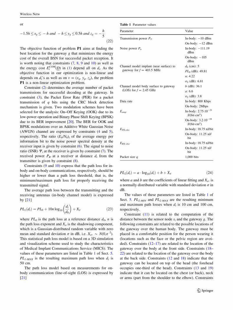
First, the effects of different modulation schemes (BPSK

and OOK) on the BER for BSNs have been analyzed. In

Fig. 3 the BER is shown as a function of the distance

between a body surface node and the gateway in an on-

BSN. For a target BER the hop length is extended using

BPSK modulation compared to OOK modulation. For a

particular hop distance, the BER is lower for BPSK than

for OOK modulation. For a distance of 50 cm the BER is

100 % lower for BPSK than for OOK modulation.

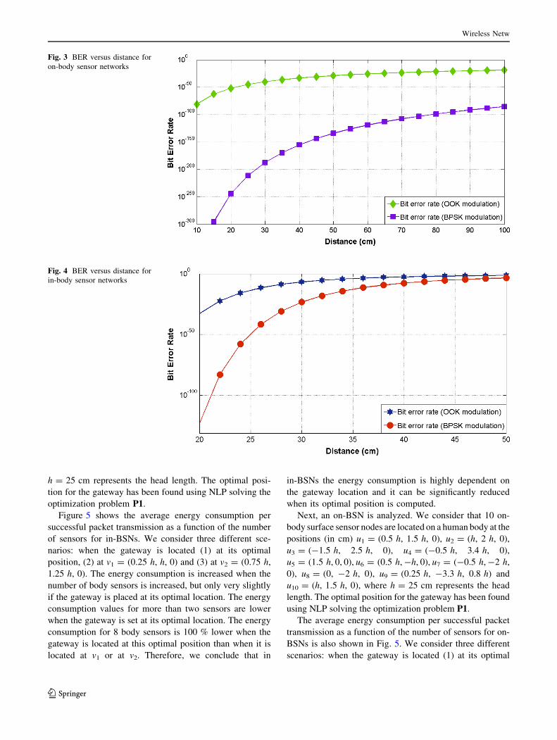
In Fig. 4 the BER is shown as a function of the distance

between an implant node and the gateway in an in-BSN.

Again the BPSK modulation results in larger hop length

extension than OOK. For a target BER of 10-4 the hop length

is extended 37.1 % using BPSK instead of OOK modulation.

BPSK has been selected as modulation scheme due to its

good performance for location optimization. BPSK is also

used as modulation scheme in [26], [27], [28] and [29].

For QPSK the data rate can be doubled compared to a

BPSK system while maintaining the same bandwidth of the

signal; another possibility is to maintain the data rate of

BPSK and halve the bandwidth.

In any case, the BER of QPSK is exactly the same as the

BER of BPSK, which means that for QPSK the location

optimization problems P1 and P2 can be solved in the same

way as if BPSK is considered.

5.2 Case 1: optimal placement evaluation

Next, case 1 has been solved numerically. It has been

assumed that the positions of each sensor node si are

determined by their functionality and can’t be changed. As

an example, a new kind of sensors could be inserted at

specific locations under the soldier’s skin to monitor

important biomarkers. The optimal location for the gate-

way needs to be found. We consider a gateway g located at

v = (xg, yg, zg), v [ X. Each body sensor si [ S is located at

ui = (xi, yi, zi), ui [ X.

First, an in-BSN is analyzed. We assume that 10 in-body

surface sensors are located in a human body at the positions

(in cm) u1 = (0.5 h, 1.5 h, -1), u2 = (h, 2 h, -1.5),

u3 = (-1.5 h, 2.5 h, -0.5), u4 = (-0.5 h, 3.4 h, -1),

u5 = (1.5 h, 1.5 h, -1.5), u6 = (0.5 h, h, -0.5), u7 =

(-0.5 h, 0.5 h, -0.5), u8 = (h, 0.5 h, -1.5), u9 = (-h,

0.5 h, -1) and u10 = (-1.5 h, 0.35 h, -0.5), where

Wireless Netw

123

h = 25 cm represents the head length. The optimal posi-

tion for the gateway has been found using NLP solving the

optimization problem P1.

Figure 5 shows the average energy consumption per

successful packet transmission as a function of the number

of sensors for in-BSNs. We consider three different sce-

narios: when the gateway is located (1) at its optimal

position, (2) at v1 = (0.25 h, h, 0) and (3) at v2 = (0.75 h,

1.25 h, 0). The energy consumption is increased when the

number of body sensors is increased, but only very slightly

if the gateway is placed at its optimal location. The energy

consumption values for more than two sensors are lower

when the gateway is set at its optimal location. The energy

consumption for 8 body sensors is 100 % lower when the

gateway is located at this optimal position than when it is

located at v1 or at v2. Therefore, we conclude that in

in-BSNs the energy consumption is highly dependent on

the gateway location and it can be significantly reduced

when its optimal position is computed.

Next, an on-BSN is analyzed. We consider that 10 on-

body surface sensor nodes are located on a human body at the

positions (in cm) u1 = (0.5 h, 1.5 h, 0), u2 = (h, 2 h, 0),

u3 = (-1.5 h, 2.5 h, 0), u4 = (-0.5 h, 3.4 h, 0),

u5 = (1.5 h, 0, 0), u6 = (0.5 h, -h, 0), u7 = (-0.5 h, -2 h,

0), u8 = (0, -2 h, 0), u9 = (0.25 h, -3.3 h, 0.8 h) and

u10 = (h, 1.5 h, 0), where h = 25 cm represents the head

length. The optimal position for the gateway has been found

using NLP solving the optimization problem P1.

The average energy consumption per successful packet

transmission as a function of the number of sensors for on-

BSNs is also shown in Fig. 5. We consider three different

scenarios: when the gateway is located (1) at its optimal

Fig. 3 BER versus distance for

on-body sensor networks

Fig. 4 BER versus distance for

in-body sensor networks

Wireless Netw

123

position, (2) at v1 = (-h, -3 h,0) and 3) at v2 = (0.5 h,

3.5 h, 0). The energy consumption is increased when the

number of body sensors is increased. The energy con-

sumption values when the gateway is set at its optimal

position, at v1 or at v2 are exactly the same. The reason is

that for the transmission ranges between the sensor nodes

and the gateway (between 10 and 100 cm) the path losses

are low, the SNR is increased and consequently the BER

for BPSK is insignificant, which results in PERs of zero.

The energy consumption values are lower for on-body

than for in-body communication, although the differences

are small when the gateway is set at its optimal location for

in-body transmission. For 7 sensor nodes, the energy con-

sumption (optimal position of the gateway) is 66.98 %

higher for in-body than for on-body communication due to

the higher bit error rates.

5.3 Case 2: optimal placement evaluation

Next, case 2 has been solved numerically. It has been

assumed that the position of the gateway is determined and

can’t be changed. The positions of the sensor nodes can be

selected between certain ranges of locations depending on

their functionality; their optimal locations need to be

found. We consider a gateway g located at v = (xg, yg, zg),

v [ X. 5 body sensor nodes si [ S are located in 5 different

regions Xi.

First, an in-BSN is analyzed. We assume that the gate-

way is located in a human body at the position (in cm)

v = (-h, h,0), where h = 25 cm represents the head

length. 5 sensor nodes s1, s2, s3, s4 and s5 are located at u1 [X1, u2 [ X3, u3 [ X4, u4 [ X5 and u5 [ X6. The optimal

positions for the sensors have been found using NLP

solving the optimization problem P2.

Figure 6 shows the average energy consumption per

successful packet transmission as a function of the number

of sensors for in-BSNs. We consider two different sce-

narios: when the sensor nodes are located (1) at their

optimal positions, (2) at u1 = (-0.5 h, 3.5 h, -0.5),

u2 = (-1.25 h, -h, -1), u3 = (h, 0, -0.5), u4 =

(-h, -1.5 h, -1.5) and u5 = (0, -1.5 h, -2). The energy

consumption values are increased when the number of

Fig. 5 Energy consumption as

a function of the number of

sensors

Fig. 6 Energy consumption as

a function of the number of

sensors

Wireless Netw

123

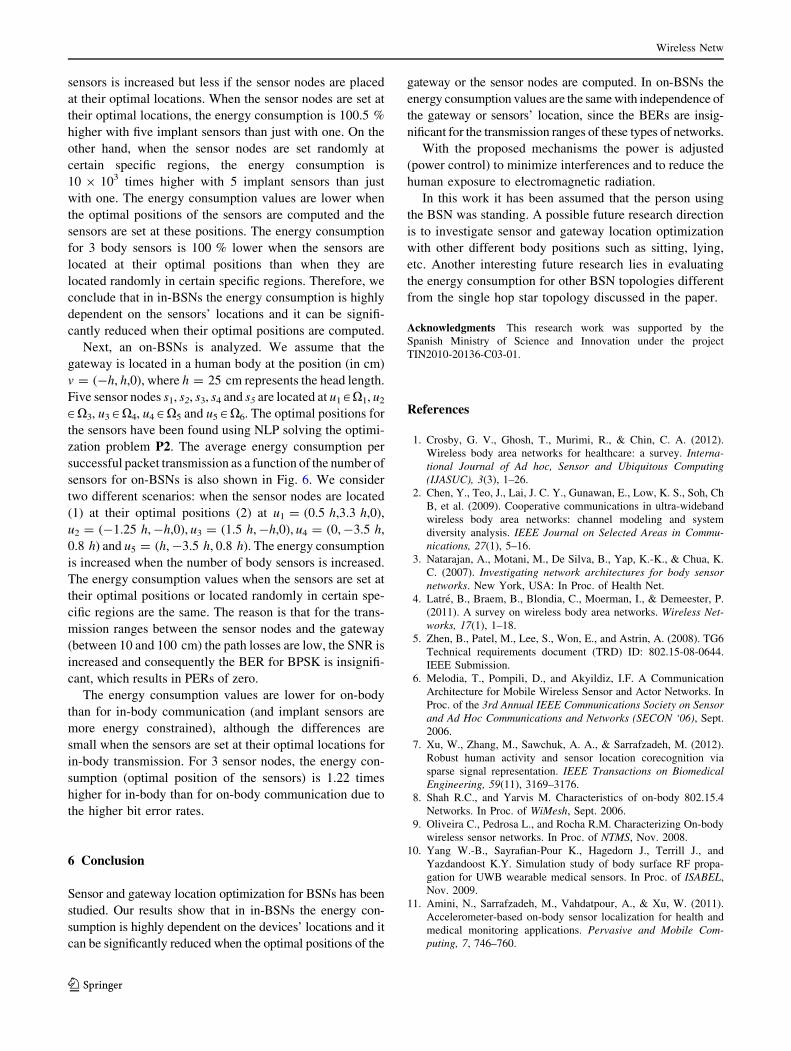
sensors is increased but less if the sensor nodes are placed

at their optimal locations. When the sensor nodes are set at

their optimal locations, the energy consumption is 100.5 %

higher with five implant sensors than just with one. On the

other hand, when the sensor nodes are set randomly at

certain specific regions, the energy consumption is

10 9 103 times higher with 5 implant sensors than just

with one. The energy consumption values are lower when

the optimal positions of the sensors are computed and the

sensors are set at these positions. The energy consumption

for 3 body sensors is 100 % lower when the sensors are

located at their optimal positions than when they are

located randomly in certain specific regions. Therefore, we

conclude that in in-BSNs the energy consumption is highly

dependent on the sensors’ locations and it can be signifi-

cantly reduced when their optimal positions are computed.

Next, an on-BSNs is analyzed. We assume that the

gateway is located in a human body at the position (in cm)

v = (-h, h,0), where h = 25 cm represents the head length.

Five sensor nodes s1, s2, s3, s4 and s5 are located at u1 [X1, u2

[ X3, u3 [ X4, u4 [ X5 and u5 [ X6. The optimal positions for

the sensors have been found using NLP solving the optimi-

zation problem P2. The average energy consumption per

successful packet transmission as a function of the number of

sensors for on-BSNs is also shown in Fig. 6. We consider

two different scenarios: when the sensor nodes are located

(1) at their optimal positions (2) at u1 = (0.5 h,3.3 h,0),

u2 = (-1.25 h, -h,0), u3 = (1.5 h, -h,0), u4 = (0, -3.5 h,

0.8 h) and u5 = (h, -3.5 h, 0.8 h). The energy consumption

is increased when the number of body sensors is increased.

The energy consumption values when the sensors are set at

their optimal positions or located randomly in certain spe-

cific regions are the same. The reason is that for the trans-

mission ranges between the sensor nodes and the gateway

(between 10 and 100 cm) the path losses are low, the SNR is

increased and consequently the BER for BPSK is insignifi-

cant, which results in PERs of zero.

The energy consumption values are lower for on-body

than for in-body communication (and implant sensors are

more energy constrained), although the differences are

small when the sensors are set at their optimal locations for

in-body transmission. For 3 sensor nodes, the energy con-

sumption (optimal position of the sensors) is 1.22 times

higher for in-body than for on-body communication due to

the higher bit error rates.

6 Conclusion

Sensor and gateway location optimization for BSNs has been

studied. Our results show that in in-BSNs the energy con-

sumption is highly dependent on the devices’ locations and it

can be significantly reduced when the optimal positions of the

gateway or the sensor nodes are computed. In on-BSNs the

energy consumption values are the same with independence of

the gateway or sensors’ location, since the BERs are insig-

nificant for the transmission ranges of these types of networks.

With the proposed mechanisms the power is adjusted

(power control) to minimize interferences and to reduce the

human exposure to electromagnetic radiation.

In this work it has been assumed that the person using

the BSN was standing. A possible future research direction

is to investigate sensor and gateway location optimization

with other different body positions such as sitting, lying,

etc. Another interesting future research lies in evaluating

the energy consumption for other BSN topologies different

from the single hop star topology discussed in the paper.

Acknowledgments This research work was supported by the

Spanish Ministry of Science and Innovation under the project

TIN2010-20136-C03-01.

References

1. Crosby, G. V., Ghosh, T., Murimi, R., & Chin, C. A. (2012).

Wireless body area networks for healthcare: a survey. Interna-

tional Journal of Ad hoc, Sensor and Ubiquitous Computing

(IJASUC), 3(3), 1–26.

2. Chen, Y., Teo, J., Lai, J. C. Y., Gunawan, E., Low, K. S., Soh, Ch

B, et al. (2009). Cooperative communications in ultra-wideband

wireless body area networks: channel modeling and system

diversity analysis. IEEE Journal on Selected Areas in Commu-

nications, 27(1), 5–16.

3. Natarajan, A., Motani, M., De Silva, B., Yap, K.-K., & Chua, K.

C. (2007). Investigating network architectures for body sensor

networks. New York, USA: In Proc. of Health Net.

4. Latre, B., Braem, B., Blondia, C., Moerman, I., & Demeester, P.

(2011). A survey on wireless body area networks. Wireless Net-

works, 17(1), 1–18.

5. Zhen, B., Patel, M., Lee, S., Won, E., and Astrin, A. (2008). TG6

Technical requirements document (TRD) ID: 802.15-08-0644.

IEEE Submission.

6. Melodia, T., Pompili, D., and Akyildiz, I.F. A Communication

Architecture for Mobile Wireless Sensor and Actor Networks. In

Proc. of the 3rd Annual IEEE Communications Society on Sensor

and Ad Hoc Communications and Networks (SECON ‘06), Sept.

2006.

7. Xu, W., Zhang, M., Sawchuk, A. A., & Sarrafzadeh, M. (2012).

Robust human activity and sensor location corecognition via

sparse signal representation. IEEE Transactions on Biomedical

Engineering, 59(11), 3169–3176.

8. Shah R.C., and Yarvis M. Characteristics of on-body 802.15.4

Networks. In Proc. of WiMesh, Sept. 2006.

9. Oliveira C., Pedrosa L., and Rocha R.M. Characterizing On-body

wireless sensor networks. In Proc. of NTMS, Nov. 2008.

10. Yang W.-B., Sayrafian-Pour K., Hagedorn J., Terrill J., and

Yazdandoost K.Y. Simulation study of body surface RF propa-

gation for UWB wearable medical sensors. In Proc. of ISABEL,

Nov. 2009.

11. Amini, N., Sarrafzadeh, M., Vahdatpour, A., & Xu, W. (2011).

Accelerometer-based on-body sensor localization for health and

medical monitoring applications. Pervasive and Mobile Com-

puting, 7, 746–760.

Wireless Netw

123

12. Atallah, L., Lo, B., King, R., & Yang, G.-Z. (2011). Sensor

positioning for activity recognition using wearable accelerome-

ters. IEEE Transactions on Biomedical Circuits and Systems,

5(4), 320–329.

13. Min, Ch-H, Tewfik, A. H., Kim, Y., & Menard, R. (2009).

Optimal sensor location for body sensor network to detect self-

stimulatory behaviors of children with autism spectrum disorder.

Sept: In Proc. of EMBC.

14. Patterson, J.A.C., McIlwraith, D.G., and Yang, G.-Z. A Flexible,

Low Noise Reflective PPG Sensor Platform for Ear-Worn Heart

Rate Monitoring. In Proc. of BSN, June 2009.

15. Zhao, G., Mei, Z., Liang, D., Ivanov, K., Guo, Y., Wang, Y., et al.

(2012). Exploration and implementation of a pre-impact fall

recognition method based on an inertial body sensor network.

Sensors (Basel), 12(11), 15338–15355.

16. Atallah, L., Aziz, O., Lo, B., and Yang, G.-Z., Detecting Walking

Gait Impairment with an Ear-worn Sensor, in Proc. of BSN, June

2009.

17. Jovanov, E., Milenkovic, A., Otto, C., & de Groen, P. C. (2005).

A wireless body area network of intelligent motion sensors for

computer assisted physical rehabilitation. Journal of NeuroEn-

gineering and Rehabilitation, 2(1), 16–23.

18. Standards for Measurement of the Human Body. Available at:

http://www2.evansville.edu/drawinglab/proportion.html.

19. Reusens, E., Joseph, W., Latre, B., Braem, B., Vermeeren, G.,

Tanghe, E., et al. (2009). Characterization of on-body commu-

nication channel and energy efficient topology design for wireless

body area networks. IEEE Transactions of Information Tech-

nology in Biomedicine, 13(6), 933–945.

20. Takizawa, K., Aoyagi, T., and Kohno, R. Channel Modeling and

Performance Evaluation of UWB-based Wireless Body Area

Networks. In Proc. of ICC 2009, June 2009.

21. Yazdandoost, K.Y., and Sayrafian-Pour, K. Channel Model for

Body Area Network (BAN). Report to the IEEE P802.15, ID:

IEEE P802.15-08-0780-12-0006, November 2010.

22. Byrd, R. H., Hribar, M. E., & Nocedal, J. (1999). An interior

point algorithm for large scale nonlinear programming. SIAM

Journal of Optimization, 9, 877–900.

23. Gill, P. E., Murray, W., & Saunders, M. A. (2005). SNOPT: An

SQP algorithm for large-scale constrained optimization. SIAM

Review, 47(1), 99–131.

24. Zarlink ZL70101. Datasheet available at: http://www.zarlink.

com/zarlink/.

25. Nordic nRF24L01 ? . Datasheet available at: http://www.nor

dicsemi.com/.

26. Sasamori, T., Satoh, Y., Tobana, T., Isota, Y., Takahashi, M., and

Uno T. Bit Error rate performance of wireless body area network

system. In Proc. of IEEE Antennas and Propagation Society

International Symposium (APSURSI), July 2010.

27. Seunghyun, Oh, and Wentzloff, D.D. Portable hardware for real-

time channel estimation on wireless body Area networks. In Proc.

of Biomedical Circuits and Systems Conference (BioCAS), Nov.

2011.

28. Hsieh, C.-H., Su M.Y., Kung, J.-Y., Lee S.-Y., and Fang, Q. Low-

power 13.56 MHz RF Front-end Circuit for Body Sensor Net-

work, In Proc. of International Symposium on Bioelectronics and

Bioinformatics (ISBB), Nov. 2011.

29. Chen, X., Lu, X., Jin, D., Su, Li, and Zeng, L. Channel modeling

of UWB-based wireless body area networks, In Proc. of IEEE

International Conference on Communications (ICC), June 2011.

Mari Carmen Domingoreceived her Lic. degree in

Electrical Engineering and her

Ph.D. in Electrical Engineering

from the Barcelona Tech Uni-

versity, Barcelona, Spain in

1999 and 2005, respectively.

She currently works as Assistant

Professor at the Electrical

Engineering Department. Her

current research interests are in

the area of underwater and body

sensor networks. She received

the ALCATEL ‘‘Best Ph.D.

thesis in wired-wireless conver-

gence: applications and services’’ award from the Spanish Telecom-

munication Engineers Official Association (COIT) in 2006. From

February to October 2008, she has been a postdoctoral researcher at

the Broadband Wireless Networking Laboratory, Georgia Institute of

Technology, Atlanta, Georgia, USA.

Wireless Netw

123