Sensitivity of the CRCM Atmospheric and the Gulf of St. Lawrence Ocean–Ice Models to Each Other

Manon Faucher1*, Daniel Caya2, François J. Saucier3 and René Laprise4

1Service Météorologique du Canada, 550 Sherbrooke Ouest, 19ième étage Montréal, QC H3A 1B9

2OURANOS, Montréal, QC3Institut Maurice-Lamontagne, Mont-Joli, QC

4UQÀM, Montréal, QC

[Original manuscript received 21 January 2003; in revised form 29 October 2003]

ABSTRACT The sensitivity of the Canadian Regional Climate Model (CRCM), developed at the Université duQuébec à Montréal, and the Gulf of St. Lawrence Ocean Model (GOM), developed at the Institut Maurice-Lamontagne, to each other is tested with an ensemble of simulations over eastern Canada from 1 November 1989to 31 March 1990. The goal of this study is to investigate the interaction of the CRCM and GOM with respect toeach other’s forcing fields. In the first part of the experiment, a series of simulations were performed using an iterative strategy, where both models run separately and alternately, using variables from the other model to supply the needed forcing fields for the computation of surface fluxes. The runs are iterated several times over thesame period from the output of the previous run to allow the atmosphere and the ocean to interact several timeswith each other and to study the evolution of the solutions from one iteration to the next. In the second part of theexperiment, a two-way coupled simulation is performed over the same period. The results indicate that on a monthlyor longer timescale, the CRCM is not very sensitive to the details of the oceanic fields from GOM, except locally overthe Gulf of St. Lawrence (GSL). However, GOM is quite sensitive to the differences in atmospheric fields from theCRCM. The results of several iterations converge to a unique solution, suggesting that the CRCM and GOM reachequilibrium with respect to each other’s forcing fields. Furthermore, the results of the coupled run also convergeto this same solution.

RÉSUMÉ Nous testons la sensibilité du modèle régional Canadien de climat (MRCC, développé à l’université duQuébec à Montréal) et d’un modèle océanique du golfe du Saint-Laurent (MOG, développé à l’institut Maurice-Lamontagne) l’un par rapport à l’autre avec un ensemble de simulations pour l’est du Canada. La période dessimulations est du 1er novembre 1989 au 31 mars 1990. Le but de ce travail est l’étude de l’interaction du MRCCet du MOG l’un par rapport aux champs de surface de l’autre. Dans la première partie de l’expérience, une sériede simulations ont été faites à partir d’une stratégie itérative d’échange de données. Selon cette stratégie, les deuxmodèles fonctionnent séparement et alternativement en utilisant les variables de l’autre modèle pour obtenir leschamps nécessaires. Les simulations sont itérées plusieurs fois sur la même période à partir des champs issus dela simulation précédente pour permettre à l’atmosphère et l’océan d’interagir plusieurs fois l’un avec l’autre etpour étudier l’évolution des simulations d’une itération à la suivante. Dans la deuxième partie de l’expérience,nous exécutons une simulation couplée bi-directionnelle sur la même période d’étude. Les résultats indiquentqu’à l’échelle mensuelle ou à plus long terme, le MRCC n’est pas très sensible aux détails des conditionsocéaniques de MOG, sauf localement au-dessus du golfe du Saint-Laurent. Cependant, MOG est très sensible auxdifférences des champs atmosphériques du MRCC. Les résultats de plusieurs itérations convergent vers une solutionunique, ce qui suggère que le MRCC et le MOG atteignent l’équilibre par rapport aux champs de surface de chacun des modèles. De plus, les résultats de la simulation couplée convergent aussi vers cette même solution.

ATMOSPHERE-OCEAN 42 (2) 2004, 85–100© Canadian Meteorological and Oceanographic Society

*Corresponding author: manon.faucher@ec.gc.ca

1 IntroductionThe climate of eastern Canada is influenced by the atmos-phere–ocean interaction due to the proximity of the LabradorSea and the North Atlantic Ocean. Also, three relatively largeinner basins: the Gulf of St. Lawrence (GSL), the HudsonBay/Hudson Strait/Foxe Basin system and the Great Lakes

interact with the atmosphere. These basins are characterizedby variable sea ice in winter and irregular coastlines modulat-ing heat and moisture fluxes from the ocean over relativelyshort space and time scales. With climate change issues, thereis a need to understand further the climate system in eastern

Canada, including the role of the interaction of the atmos-phere, the ocean and the sea ice.

The study of the climate requires sophisticated models ofthe atmosphere, ocean and sea ice because each component ofthe system interacts with the others in complex ways. CoupledGlobal Climate Models (GCMs) are available to study the cli-mate of eastern Canada, but their resolution (typically 350 km)is too coarse either to resolve the details of the regional climateof our area of interest properly or to provide valuable infor-mation for climate impact studies. In Canada, we have aregional climate model that can be applied anywhere on theplanet, the Canadian Regional Climate Model (CRCM) devel-oped at the Université du Québec à Montréal (Caya, 1996;Caya and Laprise, 1999), and we have regional ocean–icemodels for various oceanic domains. In particular, ocean–icemodels have been developed for the GSL (Gulf of St.Lawrence Ocean Model (GOM)) and for Hudson Bay at theMaurice Lamontagne Institute (Saucier et al., 2003a; Saucieret al., 2003b) to study the ocean dynamics of the respectivebasins. These models were developed independently and areroutinely used independently. However, we are now starting tocouple the CRCM with different oceanic components toinclude the feedbacks of the atmosphere–ocean–ice system inatmospheric and oceanic simulations. In order to make futureclimate projections, the coupling of atmospheric and oceaniccomponents is necessary to develop a consistent regional cli-mate model system that is independent of any database.

While the complex problem of a full coupling is avoidedhere, this paper addresses the interaction of the CRCM withan ocean–ice model for the GSL as a first step in the devel-opment of the coupled regional climate model for easternCanada. The main objective of this paper is two-fold. Firstly,test the general sensitivity of the simulated CRCM and GOMsolutions to each other before engaging the models in a fullycoupled mode. Since the models were developed indepen-dently and run with low-resolution observations at the air–seaboundary, it is unclear how the models may react once theseobservations are replaced by relatively high resolution simu-lated atmospheric or ocean–ice data at the air–sea boundary.Secondly, perform a two-way coupled simulation for thesame period and compare the solution with those of uncou-pled but interacting simulations by the two models. Theobjective involves studying the impact of atmosphere–ocean–ice interactions on the atmospheric and oceanic circulationand looking at the solutions on a monthly or longer timescale.A question to address in this paper is the need to bring a three-dimensional (3-D) high-resolution oceanic model into theCRCM for climate applications in the GSL area by studyingtheir response to each other from a series of iterative runs.While previous studies by Saucier et al. (2003a), Roy et al.(1999) and Besner (1999) indicate the importance of relative-ly high-resolution atmospheric forcing fields for GOM, theinfluence of high-resolution ocean surface conditions in theCRCM as opposed to GCM forcing fields, for example, hasnot yet been studied.

Research efforts devoted to the coupling of regional cli-mate models (RCMs) with dynamic ocean models to improveclimate simulations are underway in other parts of the world.For example, at the Rossby Centre in Sweden a regional cou-pled atmosphere–ocean–ice model is being developed fornorthern Europe with an interactive coupling over the Baltic

Sea (Döscher et al., 2002). This project is part of the BalticSea Experiment (BALTEX). At the University of Colorado,the National Center for Atmospheric Research (NCAR)regional climate model, RegCM2, has been coupled to anocean–ice model to improve the simulated regional climate ofthe Arctic (ARCSym; Lynch et al., 1995).

In eastern Canada, the coupling of the CRCM over the GSLis an interesting problem because of observed atmosphere–ocean–ice interactions that may affect both the atmosphericand oceanic dynamics–thermodynamics. Also, the climate ofthe GSL is relatively well documented, which will help withthe interpretation of our results. The GSL is a semi-enclosedsea connected to the North Atlantic Ocean through CabotStrait to the south-east and through the Strait of Belle-Isle tothe north-east (Fig. 1). Its estuary extends from Pointe-des-Monts towards the upstream limit of salt intrusion nearQuébec City and even toward Lake Saint-Pierre in the St.Lawrence River (between Québec City and Montréal).Wintertime low-pressure systems propagating from the GreatLakes or from the Gulf of Mexico may be strengthened whenthey receive additional moisture and heat as they reach theGSL in unfrozen conditions. When the Gulf is ice-covered thesea ice damps the interaction between the atmosphere and theocean because of its reflective and insulating properties.Typically, sea ice begins to form in the St. Lawrence Estuaryand the north-west section of the GSL by mid-December; itspreads over much of the GSL by the end of January andbegins to melt in March (Koutitonsky and Bugden, 1991).However, sea ice is subject to dynamical forces and is not acontinuous medium. The combined effect of winds and tidescan fracture the ice creating large areas of open water, whichincrease the sensible and latent heat fluxes locally. When thishappens, sensible heat fluxes can reach 1000 W m–2 (heat lostfrom the ocean) locally near the coast compared to the typicalmean winter values of 250 W m–2 presented in Koutitonskyand Bugden (1991). Such large surface heat fluxes result inthe development of atmospheric convective instability overopen water. This instability may be responsible for significantsnowfall over adjacent areas.

The sensitivity of the CRCM-simulated weather systems tothe GSL ocean surface conditions has recently been investi-gated with a short uncoupled simulation for the first week ofJanuary 1990. Using two different ice regimes representingminimum and maximum observed ice extent, the authorsshow that the regional atmospheric circulation in winter issensitive to the observed variability in the surface oceanicconditions in the GSL, especially during a cyclone event.Moreover, their study indicates that differences in the icecover perturb the low-level atmospheric fields from the GSLtowards the east and north-east, along the cyclone track. Theauthors also performed a coupled experiment with the CRCMand GOM for the same week in January 1990 (Gachon et al.,2001). Their results indicate that the change in sea ice duringthe period of integration generates a modification in the sur-face heating over the GSL, which in turn modifies the region-al low-level winds and temperature. The response of theCRCM was found to be important locally over the GSL, innorthern Quebec and over the Labrador Sea. The authorsreport that ‘The cumulative effects of the mesoscale pattern ofatmospheric circulation due to the sea surface conditions inthe GSL could modify the climate variability in numerical

86 / Manon Faucher et al.

simulation at regional scales, in the context of rapid andintense winter variation in sea ice cover, as it is regularlyobserved in the GSL.’ However, this has to be tested on a sea-sonal or annual timescale taking into account the internalvariability of the models.

In this paper, we will look at the sensitivity of the CRCMand GOM regional models to each other with an ensemble ofatmospheric and oceanic simulations. These simulations areperformed over a winter season and integrate the effect of aseries of weather systems over eastern Canada. A first CRCMsimulation begins the experiment, where observations fromthe Atmospheric Model Intercomparison Project (AMIP) IIdatabase (Gates, 1992) are interpolated to provide the ocean-ic fields over the GSL. Then, GOM uses the atmosphericfields from the CRCM run. The procedure is repeated andboth models are run separately and alternately for the entireperiod, using variables from the other model to supply theneeded fields. The variables are exchanged after each simula-tion is completed (each run is made over the same period offive months: from 1 November 1 1989 to 31 March 1990).

We performed this iterative uncoupled strategy to obtain afirst indication of the sensitivity of the CRCM and GOM toeach other. A cold anomaly is introduced initially in the AMIPII surface data to study the evolution of this anomaly throughthe iterations. In order to further the investigation, the twomodels are run in a two-way coupled simulation over the sameperiod. In this coupled simulation, the data are exchanged oncea day during the five-month period and the solution is com-pared with the previous uncoupled simulations.

The present paper is organized as follows: the experimen-tal set-up is presented in Section 2, including a short descrip-tion of the CRCM and GOM with a description of the strategyfor the exchange of the data for our sensitivity study and theexperimental configuration. The results are presented inSection 3, including the simulated atmosphere and ocean–icesystem for each run, followed by a conclusion in Section 4.

2 Experimental set-upa Atmospheric ModelThe CRCM is a limited-area model based on the fully elastic,non-hydrostatic Euler equations. Its physical parametrizationof the subgrid-scale processes is described in McFarlane et al.(1992). It includes turbulent surface fluxes of heat, momen-tum and fresh water calculated from atmospheric variables atits lowest thermodynamic level and surface variables usingbulk aerodynamic formulae as a function of a Richardsonnumber. A full description of the CRCM can be found inCaya and Laprise (1999) and its simulated climate is present-ed in Laprise et al. (1998).

Over the ocean, sea-surface temperature (SST) and sea-icefraction (SIF) must be supplied to compute the surface budgetof heat, momentum and water vapour at the interface betweenthe atmosphere and the ocean–ice system. The surface tem-perature of sea ice is calculated from the heat budget. SST andSIF can be supplied to the CRCM from observations or frommodel outputs. However, the temporal and spatial resolutionsof the databases are too low to resolve the details of the sur-face characterized by the highly complex coastlines and

Atmosphere–Ocean – Ice Interactions over the Gulf of St. Lawrence / 87

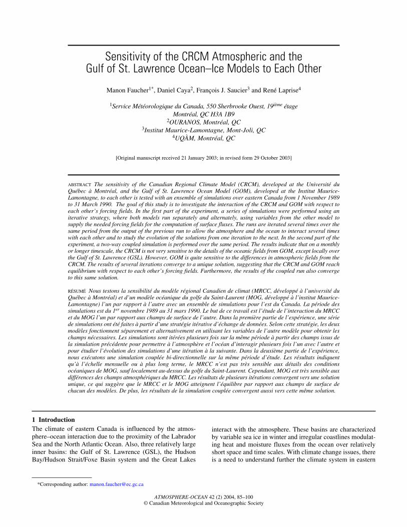
Fig. 1 Model domain for the CRCM with the land–sea mask and topographical height (contours every 100 m). The CRCM sponge zone is excluded and theGOM’s domain is indicated by a black rectangle. The land. the ocean and the sea ice are in dark grey, light grey and white respectively. NF indicates theprovince of Newfoundland, G.P. is the Gaspé Peninsula and A.I. is Anticosti Island.

sea-ice coverage of eastern Canada. Long time series of high-resolution observations are not available and, even if suchdata were available, observations can only be used for currentclimate simulations and are not suitable for performing cli-mate-change studies. Therefore, bringing an ocean–ice com-ponent into the CRCM is necessary.

b Ocean-Ice ModelThe GOM is a three-dimensional, high-resolution dynamicocean model for the Gulf of St. Lawrence and the St.Lawrence Estuary, based on hydrostatic and Boussinesqapproximations. The horizontal viscosity and diffusivity coef-ficients follow a formulation by Smagorinsky (1963). Theturbulence is resolved with a 2.0 closure model. The GOMincludes a dynamic-thermodynamic ice component based ona multi-category particle-in-cell method (Flato and Hibler,1992; Flato, 1994). The calculation of the net surface heatflux is based on a formulation of Parkinson and Washington(1979). The turbulent surface fluxes of heat, momentum andfresh water are calculated from atmospheric variables andocean–ice model surface variables using bulk aerodynamicformulae. The formulation follows a relatively simple repre-sentation of the atmospheric boundary layer processes as afunction of drag and heat exchange coefficients. A completedescription of GOM can be found in Saucier et al. (2003a).

Time series of seven atmospheric variables must be sup-plied to compute the surface budget of heat, momentum andwater vapour at the interface between the atmosphere and theocean–ice system. These variables are the 2-m temperatureand specific humidity, the 10-m wind, the cloud cover, the pre-cipitation and the incident solar radiation. Finding a completedatabase with all the required atmospheric variables is prob-lematic, especially for climate studies where long, continuoustime series are required. The early experiments with GOMused meteorological variables taken from a reconstructed cli-matology at 20 virtual sites in the GSL (Besner, 1999). Again,the spatial resolution was not sufficient to resolve the small-scale features of the atmospheric forcing properly around theGSL. Furthermore, these data cannot be used for climatechange scenarios so modelled data must be used.

c Exchange of Variables Between the CRCM and GOMThe exchange of variables between the two models is neces-sary to compute the surface fluxes of momentum, heat andfresh water in each model. GOM needs seven fields from theCRCM as mentioned in Section 2b. The 10-m wind compo-nents are interpolated from the lowest momentum level of theCRCM (≈130 m from the surface) using a logarithmic profile.The 2-m temperature and the specific humidity are interpolat-ed from the lowest thermodynamic level of the CRCM (≈65 mfrom the surface) assuming zero flux divergence.

The CRCM uses three fields from the GOM output: theSST, the SIF and sea-ice thickness. The GOM SIF is used todetermine the sea-ice mask for the CRCM based on a thresh-old value of 0.25. A grid cell is considered ice-covered whenthe SIF is greater than 0.25 and ice-free otherwise. Thisthreshold was determined from observations in the GSL for ashort experiment with the CRCM and GOM and corre-sponds to the beginning of the ice pack formation. TheGOM sea-ice thickness and a constant ice density (920 kgm–3) determine the sea-ice concentration (SIC) for the

CRCM ice-covered grid cells. In the CRCM environment, aslab represents the sea ice for each ice-covered grid cell,with a thickness calculated from its concentration (SIC).The ice slab may be snow-covered, which would modify theheat conductivity through the slab. The layer of sea ice andsnow determines an effective ice thickness in the CRCM,taking into account the effect of leads. A heat budget withinthe ice pack determines the temperature at the surface of theice. More details are given in McFarlane et al. (1992) for theCRCM ice treatment.

Outside the domain of the GOM, CRCM SST and SIF aretaken from the AMIP II database (Gates, 1992) with a resolu-tion of 1° × 1° on a latitude-longitude grid. The AMIP IImonthly average values are interpolated to supply daily val-ues to the CRCM. The values of SIC in kg m–2 are construct-ed using the National Centers for Environmental Prediction(NCEP) air temperature at 1000-hPa and AMIP SIF, follow-ing the method used at the Canadian Climate Centre for mod-elling and analysis (CCCma, M. Lazare, 2000, personalcommunication). The surface conditions of the land (soilcharacteristics, vegetation, reference albedo, surface rough-ness, snow-masking depth) are represented by a series of geo-physical fields obtained from a global database with aresolution of 1° on a latitude-longitude grid (McFarlane et al.,1992; Caya, 1996). The topography and the land–sea maskare from the U.S. Navy database.

The archive variables generated by the CRCM and GOMcannot be used directly by the other model because of theirdifferent resolution and grid configuration. An interface hasbeen developed to prepare the variables and execute theirtransfer between the CRCM and GOM. The interface carriesout the following tasks: (1) horizontal linear interpolation oraveraging of the variables between the CRCM polar stereo-graphic and the GOM Mercator grids, (2) the rotation of thewind vectors between the different grids, and (3) the adjust-ment of land–sea masks given the different grids.

d Sensitivity ExperimentThe CRCM and GOM were developed independently, usingexternal sources of information to supply the fields that are nec-essary to compute the surface fluxes. Both models perform rel-atively well in this mode, but their performance, once themodels are linked to provide the forcing fields to each other, areunknown. The present experiment was designed to assess theresponse of the CRCM and GOM to each other’s variables. Thefirst part of the experiment consists of running both modelsalternately and independently several times for a fixed periodof five months using the output from the other model. The out-put of each model is used to supply the forcing variables at theatmosphere–ocean–ice interface to the other model at a speci-fied frequency. The process is iterated three times for a five-month period (1 November 1989 to 31 March 1990) to studythe evolution of the CRCM and GOM solutions when theatmospheric or oceanic fields are updated from the previousrun with an initial large ice cover. Each model computes itsown surface budget of momentum, heat and fresh water at theinterface between the atmosphere and the underlying surface(sea ice or seawater). The second part of the experiment is touse the same interface to run a coupled simulation for the samefive months. The first month is used as a spin-up period for this experiment.

88 / Manon Faucher et al.

e Model ConfigurationsThe computational domain of the CRCM is shown in Fig. 1with the land–sea mask and the topography. The computa-tional domain contains 99 by 99 grid points in the horizontaland there is a grid spacing of 30 km (near 0.3° true at 60°N)on a polar stereographic projection. There are 30 levels in thevertical between 131 m and 31953 m. The needed lateralboundary conditions for the CRCM (horizontal wind compo-nents, temperature, pressure and water vapour are obtainedevery 12 hours from NCEP reanalyses at T32 spectral resolu-tion, which corresponds to a resolution of approximately 450km. The NCEP wind is merged with the CRCM wind in asponge zone of nine grid points following Davies (1976),while the other fields are only supplied at the domain bound-ary. The CRCM time step is ten minutes and simulated vari-ables are archived every six hours.

The computational domain of the GOM extends fromCabot Strait to Quebec and at the head of the Saguenay Fjord(near Tadoussac), with an extension from Québec City toMontréal (Fig. 1). The horizontal resolution is 5 km on arotated-Mercator projection. The ocean is layered in the ver-tical with a uniform resolution of 5 m down to a depth of 300 m and a 10-m resolution below 300 m. The surface andbottom layers are adjusted to the water level and local depthrespectively. The bottom topography is described with a 5-kmtwo-dimensional grid for the region between the outer straitsand Île d’Orléans, while it is described with a one-dimen-sional grid from Québec City to Montréal. The water levels(tide), temperature, salinity and the eddy diffusion and vis-cosity coefficients are prescribed at open boundaries acrossthe straits of Cabot and Belle-Isle (Fig. 1). The water level isspecified from 27-tidal-harmonic constituents and monthlymean temperature and salinity are obtained from a historicaldatabase. The horizontal and vertical viscosity and diffusioncoefficients are set to zero. A zero gradient condition isapplied to all velocity components on the open boundaries.Freshwater run-off is obtained from daily observations for 28tributaries and assigned to coastal boundary cells. Initial SSTsare obtained from ship survey data in the GSL. A completedescription of the initial and boundary conditions can befound in Saucier et al. (2003a). The atmospheric forcing isprovided every six hours from the CRCM output. The GOMtime-step is five minutes for the ocean component and thirtyminutes for the ice component. The variables are archivedevery six hours.

3 Results and analysisa Uncoupled Iterations 1 ITERATION 1The experiment starts with a first CRCM simulation(CRCM1) with low-resolution oceanic data (SST and per-turbed SIF from the AMIP II database) used to provide dailyoceanic surface conditions. In Fig. 2a, we present the month-ly mean distribution of SIF for December 1989. This figureshows that, resulting from the introduced anomaly, the Gulf isfully ice-covered, on average, for this month, which is large-ly overestimated compared with observed and climatologicalmeans (Drinkwater et al. 1999). Values of SIF vary from 1.0in the estuary decreasing to 0.65 at Cabot Strait and the spa-tial distribution of SIF is quite uniform, especially in the estu-

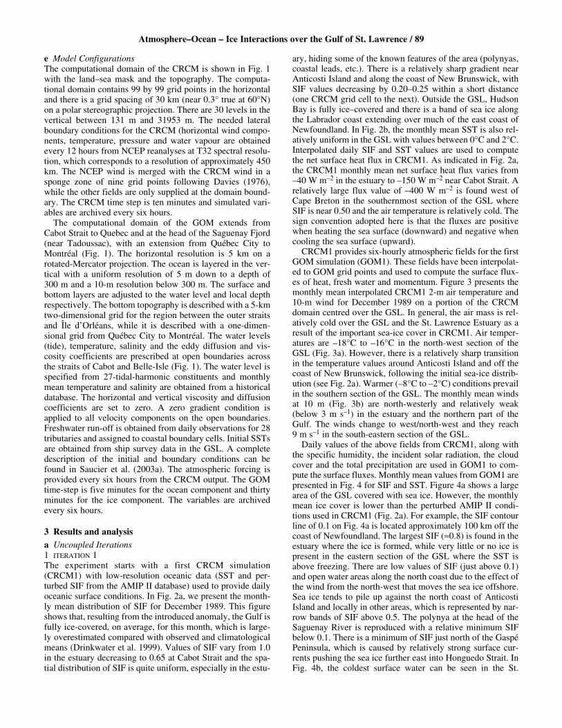
ary, hiding some of the known features of the area (polynyas,coastal leads, etc.). There is a relatively sharp gradient nearAnticosti Island and along the coast of New Brunswick, withSIF values decreasing by 0.20–0.25 within a short distance(one CRCM grid cell to the next). Outside the GSL, HudsonBay is fully ice–covered and there is a band of sea ice alongthe Labrador coast extending over much of the east coast ofNewfoundland. In Fig. 2b, the monthly mean SST is also rel-atively uniform in the GSL with values between 0°C and 2°C.Interpolated daily SIF and SST values are used to computethe net surface heat flux in CRCM1. As indicated in Fig. 2a,the CRCM1 monthly mean net surface heat flux varies from–40 W m–2 in the estuary to –150 W m–2 near Cabot Strait. Arelatively large flux value of –400 W m–2 is found west ofCape Breton in the southernmost section of the GSL whereSIF is near 0.50 and the air temperature is relatively cold. Thesign convention adopted here is that the fluxes are positivewhen heating the sea surface (downward) and negative whencooling the sea surface (upward).

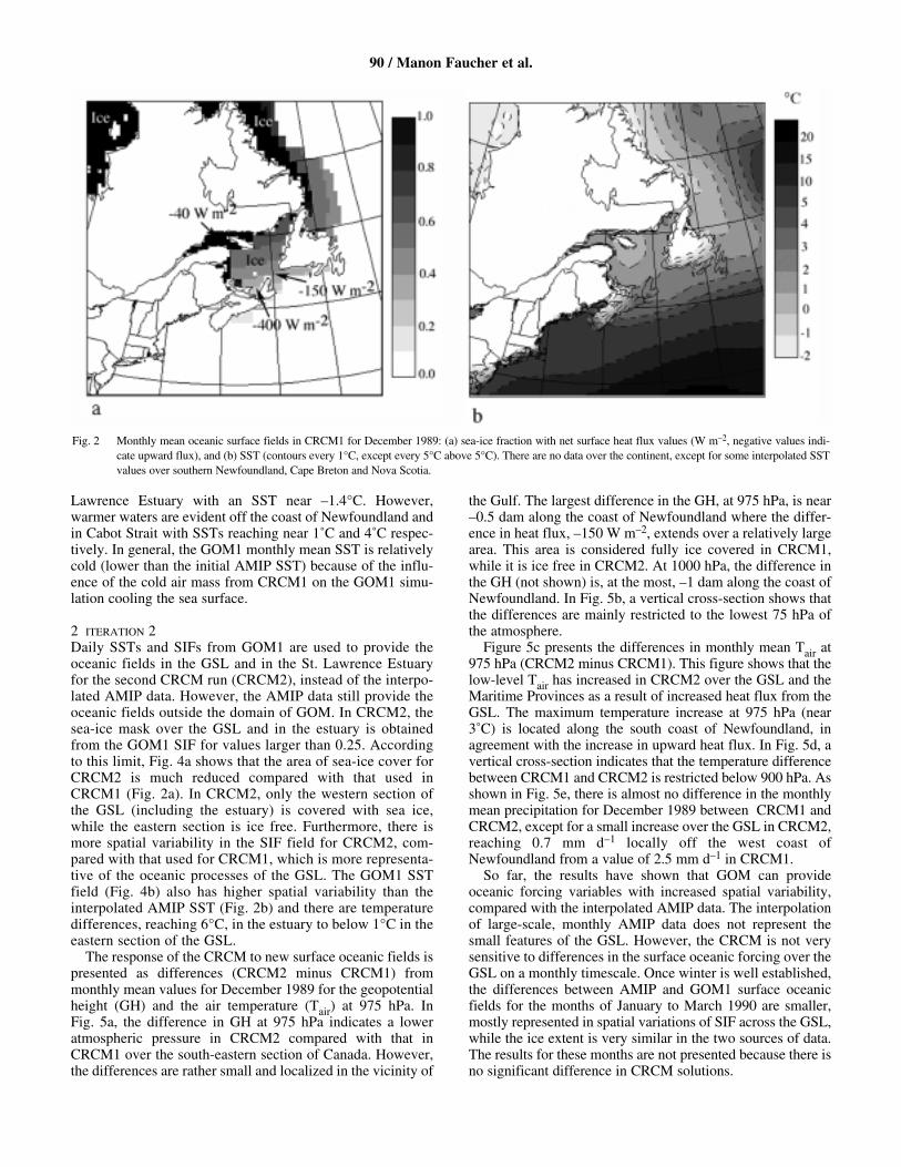
CRCM1 provides six-hourly atmospheric fields for the firstGOM simulation (GOM1). These fields have been interpolat-ed to GOM grid points and used to compute the surface flux-es of heat, fresh water and momentum. Figure 3 presents themonthly mean interpolated CRCM1 2-m air temperature and10-m wind for December 1989 on a portion of the CRCMdomain centred over the GSL. In general, the air mass is rel-atively cold over the GSL and the St. Lawrence Estuary as aresult of the important sea-ice cover in CRCM1. Air temper-atures are –18°C to –16°C in the north-west section of theGSL (Fig. 3a). However, there is a relatively sharp transitionin the temperature values around Anticosti Island and off thecoast of New Brunswick, following the initial sea-ice distrib-ution (see Fig. 2a). Warmer (–8°C to –2°C) conditions prevailin the southern section of the GSL. The monthly mean windsat 10 m (Fig. 3b) are north-westerly and relatively weak(below 3 m s–1) in the estuary and the northern part of theGulf. The winds change to west/north-west and they reach 9 m s–1 in the south-eastern section of the GSL.

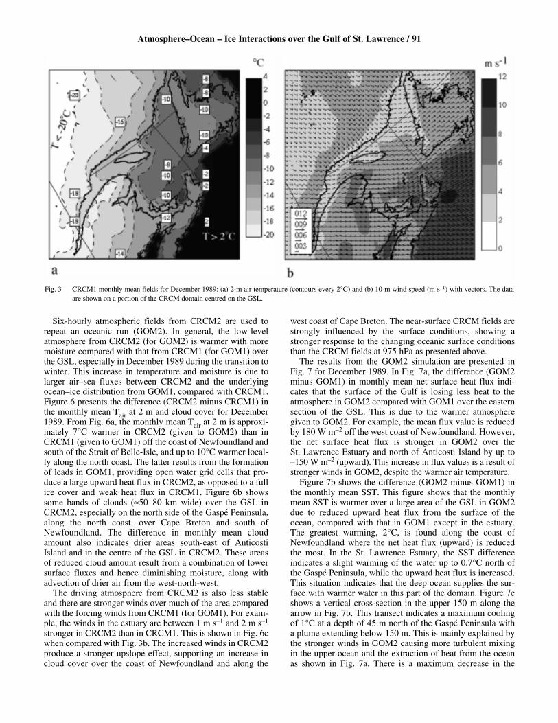
Daily values of the above fields from CRCM1, along withthe specific humidity, the incident solar radiation, the cloudcover and the total precipitation are used in GOM1 to com-pute the surface fluxes. Monthly mean values from GOM1 arepresented in Fig. 4 for SIF and SST. Figure 4a shows a largearea of the GSL covered with sea ice. However, the monthlymean ice cover is lower than the perturbed AMIP II condi-tions used in CRCM1 (Fig. 2a). For example, the SIF contourline of 0.1 on Fig. 4a is located approximately 100 km off thecoast of Newfoundland. The largest SIF (≈0.8) is found in theestuary where the ice is formed, while very little or no ice ispresent in the eastern section of the GSL where the SST isabove freezing. There are low values of SIF (just above 0.1)and open water areas along the north coast due to the effect ofthe wind from the north-west that moves the sea ice offshore.Sea ice tends to pile up against the north coast of AnticostiIsland and locally in other areas, which is represented by nar-row bands of SIF above 0.5. The polynya at the head of theSaguenay River is reproduced with a relative minimum SIFbelow 0.1. There is a minimum of SIF just north of the GaspéPeninsula, which is caused by relatively strong surface cur-rents pushing the sea ice further east into Honguedo Strait. InFig. 4b, the coldest surface water can be seen in the St.

Atmosphere–Ocean – Ice Interactions over the Gulf of St. Lawrence / 89

Lawrence Estuary with an SST near –1.4°C. However,warmer waters are evident off the coast of Newfoundland andin Cabot Strait with SSTs reaching near 1˚C and 4˚C respec-tively. In general, the GOM1 monthly mean SST is relativelycold (lower than the initial AMIP SST) because of the influ-ence of the cold air mass from CRCM1 on the GOM1 simu-lation cooling the sea surface.

2 ITERATION 2Daily SSTs and SIFs from GOM1 are used to provide theoceanic fields in the GSL and in the St. Lawrence Estuaryfor the second CRCM run (CRCM2), instead of the interpo-lated AMIP data. However, the AMIP data still provide theoceanic fields outside the domain of GOM. In CRCM2, thesea-ice mask over the GSL and in the estuary is obtainedfrom the GOM1 SIF for values larger than 0.25. Accordingto this limit, Fig. 4a shows that the area of sea-ice cover forCRCM2 is much reduced compared with that used inCRCM1 (Fig. 2a). In CRCM2, only the western section ofthe GSL (including the estuary) is covered with sea ice,while the eastern section is ice free. Furthermore, there ismore spatial variability in the SIF field for CRCM2, com-pared with that used for CRCM1, which is more representa-tive of the oceanic processes of the GSL. The GOM1 SSTfield (Fig. 4b) also has higher spatial variability than theinterpolated AMIP SST (Fig. 2b) and there are temperaturedifferences, reaching 6°C, in the estuary to below 1°C in theeastern section of the GSL.

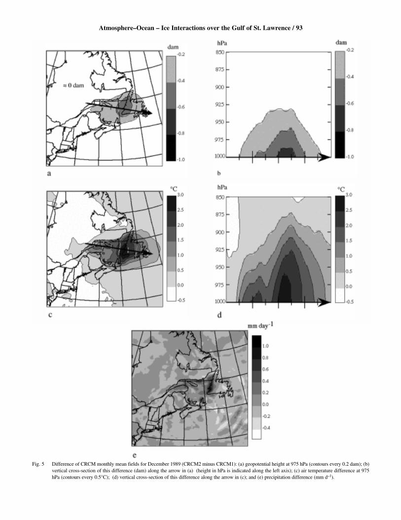
The response of the CRCM to new surface oceanic fields ispresented as differences (CRCM2 minus CRCM1) frommonthly mean values for December 1989 for the geopotentialheight (GH) and the air temperature (Tair) at 975 hPa. In Fig. 5a, the difference in GH at 975 hPa indicates a loweratmospheric pressure in CRCM2 compared with that inCRCM1 over the south-eastern section of Canada. However,the differences are rather small and localized in the vicinity of

the Gulf. The largest difference in the GH, at 975 hPa, is near–0.5 dam along the coast of Newfoundland where the differ-ence in heat flux, –150 W m–2, extends over a relatively largearea. This area is considered fully ice covered in CRCM1,while it is ice free in CRCM2. At 1000 hPa, the difference inthe GH (not shown) is, at the most, –1 dam along the coast ofNewfoundland. In Fig. 5b, a vertical cross-section shows thatthe differences are mainly restricted to the lowest 75 hPa ofthe atmosphere.

Figure 5c presents the differences in monthly mean Tair at975 hPa (CRCM2 minus CRCM1). This figure shows that thelow-level Tair has increased in CRCM2 over the GSL and theMaritime Provinces as a result of increased heat flux from theGSL. The maximum temperature increase at 975 hPa (near3˚C) is located along the south coast of Newfoundland, inagreement with the increase in upward heat flux. In Fig. 5d, avertical cross-section indicates that the temperature differencebetween CRCM1 and CRCM2 is restricted below 900 hPa. Asshown in Fig. 5e, there is almost no difference in the monthlymean precipitation for December 1989 between CRCM1 andCRCM2, except for a small increase over the GSL in CRCM2,reaching 0.7 mm d–1 locally off the west coast ofNewfoundland from a value of 2.5 mm d–1 in CRCM1.

So far, the results have shown that GOM can provideoceanic forcing variables with increased spatial variability,compared with the interpolated AMIP data. The interpolationof large-scale, monthly AMIP data does not represent thesmall features of the GSL. However, the CRCM is not verysensitive to differences in the surface oceanic forcing over theGSL on a monthly timescale. Once winter is well established,the differences between AMIP and GOM1 surface oceanicfields for the months of January to March 1990 are smaller,mostly represented in spatial variations of SIF across the GSL,while the ice extent is very similar in the two sources of data.The results for these months are not presented because there isno significant difference in CRCM solutions.

90 / Manon Faucher et al.

Fig. 2 Monthly mean oceanic surface fields in CRCM1 for December 1989: (a) sea-ice fraction with net surface heat flux values (W m–2, negative values indi-cate upward flux), and (b) SST (contours every 1°C, except every 5°C above 5°C). There are no data over the continent, except for some interpolated SSTvalues over southern Newfoundland, Cape Breton and Nova Scotia.

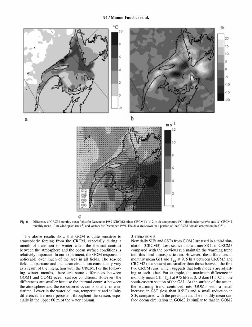
Six-hourly atmospheric fields from CRCM2 are used torepeat an oceanic run (GOM2). In general, the low-levelatmosphere from CRCM2 (for GOM2) is warmer with moremoisture compared with that from CRCM1 (for GOM1) overthe GSL, especially in December 1989 during the transition towinter. This increase in temperature and moisture is due tolarger air–sea fluxes between CRCM2 and the underlyingocean–ice distribution from GOM1, compared with CRCM1.Figure 6 presents the difference (CRCM2 minus CRCM1) inthe monthly mean Tair at 2 m and cloud cover for December1989. From Fig. 6a, the monthly mean Tair at 2 m is approxi-mately 7°C warmer in CRCM2 (given to GOM2) than inCRCM1 (given to GOM1) off the coast of Newfoundland andsouth of the Strait of Belle-Isle, and up to 10°C warmer local-ly along the north coast. The latter results from the formationof leads in GOM1, providing open water grid cells that pro-duce a large upward heat flux in CRCM2, as opposed to a fullice cover and weak heat flux in CRCM1. Figure 6b showssome bands of clouds (≈50–80 km wide) over the GSL inCRCM2, especially on the north side of the Gaspé Peninsula,along the north coast, over Cape Breton and south ofNewfoundland. The difference in monthly mean cloudamount also indicates drier areas south-east of AnticostiIsland and in the centre of the GSL in CRCM2. These areasof reduced cloud amount result from a combination of lowersurface fluxes and hence diminishing moisture, along withadvection of drier air from the west-north-west.

The driving atmosphere from CRCM2 is also less stableand there are stronger winds over much of the area comparedwith the forcing winds from CRCM1 (for GOM1). For exam-ple, the winds in the estuary are between 1 m s–1 and 2 m s–1

stronger in CRCM2 than in CRCM1. This is shown in Fig. 6cwhen compared with Fig. 3b. The increased winds in CRCM2produce a stronger upslope effect, supporting an increase incloud cover over the coast of Newfoundland and along the

west coast of Cape Breton. The near-surface CRCM fields arestrongly influenced by the surface conditions, showing astronger response to the changing oceanic surface conditionsthan the CRCM fields at 975 hPa as presented above.

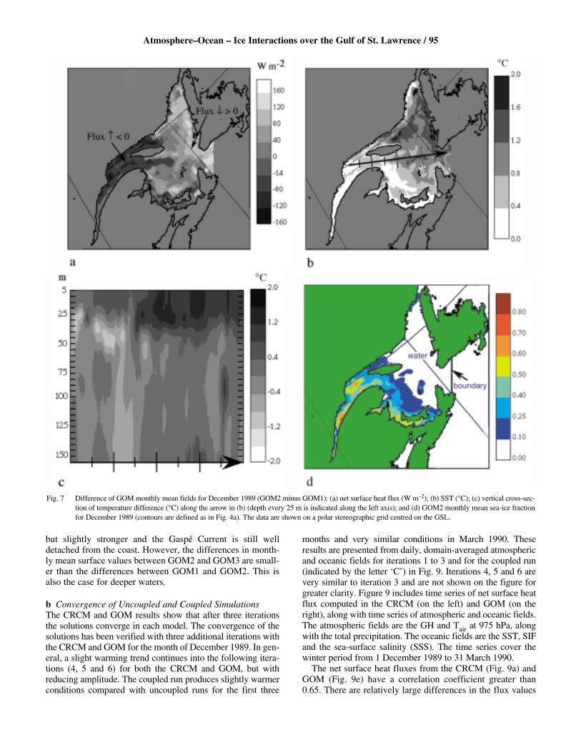
The results from the GOM2 simulation are presented inFig. 7 for December 1989. In Fig. 7a, the difference (GOM2minus GOM1) in monthly mean net surface heat flux indi-cates that the surface of the Gulf is losing less heat to theatmosphere in GOM2 compared with GOM1 over the easternsection of the GSL. This is due to the warmer atmospheregiven to GOM2. For example, the mean flux value is reducedby 180 W m–2 off the west coast of Newfoundland. However,the net surface heat flux is stronger in GOM2 over the St. Lawrence Estuary and north of Anticosti Island by up to–150 W m–2 (upward). This increase in flux values is a result ofstronger winds in GOM2, despite the warmer air temperature.

Figure 7b shows the difference (GOM2 minus GOM1) inthe monthly mean SST. This figure shows that the monthlymean SST is warmer over a large area of the GSL in GOM2due to reduced upward heat flux from the surface of theocean, compared with that in GOM1 except in the estuary.The greatest warming, 2°C, is found along the coast ofNewfoundland where the net heat flux (upward) is reducedthe most. In the St. Lawrence Estuary, the SST differenceindicates a slight warming of the water up to 0.7°C north ofthe Gaspé Peninsula, while the upward heat flux is increased.This situation indicates that the deep ocean supplies the sur-face with warmer water in this part of the domain. Figure 7cshows a vertical cross-section in the upper 150 m along thearrow in Fig. 7b. This transect indicates a maximum coolingof 1°C at a depth of 45 m north of the Gaspé Peninsula witha plume extending below 150 m. This is mainly explained bythe stronger winds in GOM2 causing more turbulent mixingin the upper ocean and the extraction of heat from the oceanas shown in Fig. 7a. There is a maximum decrease in the

Atmosphere–Ocean – Ice Interactions over the Gulf of St. Lawrence / 91

Fig. 3 CRCM1 monthly mean fields for December 1989: (a) 2-m air temperature (contours every 2°C) and (b) 10-m wind speed (m s–1) with vectors. The dataare shown on a portion of the CRCM domain centred on the GSL.

salinity of 1 g kg–1 at 55 m (not shown) associated with thispattern. Further east, the warming of the ocean is stronger inthe upper 40 m, but it extends down to 150 m with an increasein the salinity.

From Fig. 7d, the resulting monthly mean area of sea-icecover is much reduced in GOM2 compared with GOM1 (Fig. 4a). In GOM2, only the western part of the domain iscovered with sea ice and the SIF contour of 0.1 now lies acrossthe centre of the GSL. However, there is a small area of sea icestill present in the most north-easterly section. In the westernpart of the GSL and in the estuary, the SIF in GOM2 isreduced by 0.10 to 0.15 compared with the previous oceanicrun. Slightly warmer SSTs in GOM2, compared with GOM1,may explain this reduction in SIF. The sea ice is also thinnerin most coastal areas. The largest thickness difference of 10cm is found along the west coast of Anticosti Island. The effectof stronger winds in GOM2 seems to play a role in this reduc-tion of sea ice by advecting the sea ice east and south-east.

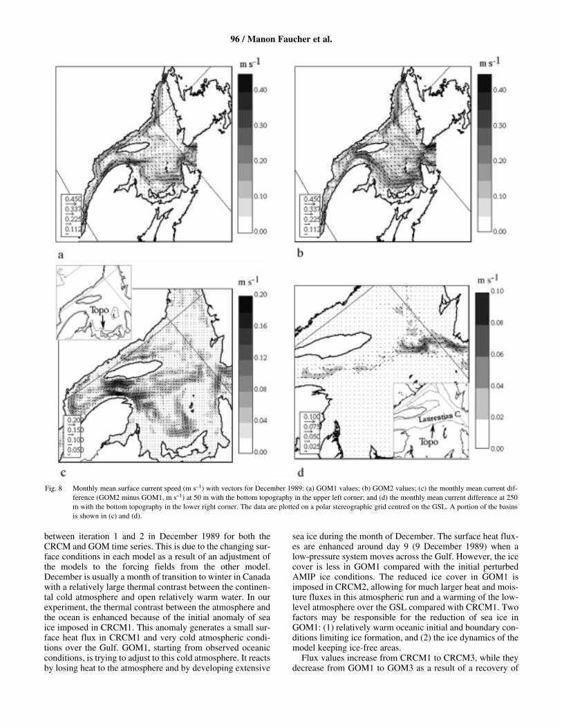
The monthly mean surface ocean currents show importantdifferences between GOM1 and GOM2 for December 1989.In Fig. 8a, the GOM1 solution shows a southward flow overthe Magdalen Shallows with a speed near 10–15 cm s–1 andthe Gaspé Current along the Gaspé Peninsula with a speednear 35 cm s–1. In Fig. 8b, the GOM2 solution shows anincreased ocean surface circulation and southward transportof water, especially in the western section of the basin. Thesouthward surface current through the Magdalen Shallows andthrough Cabot Strait reaches 25 cm s–1 to 30 cm s–1 in GOM2.The solution for the Gaspé Current is quite different in GOM2because the current splits and moves further into HonguedoStrait. Along with this structure, the Anticosti gyre that is welldeveloped in GOM1 shifts eastward and is distorted inGOM2. These two solutions for the Gaspé Current have beenobserved from current measurements and via SSTs derived

from satellite imagery (Koutitonsky and Bugden, 1991).However, the mechanisms responsible for the variability ofthis current remain unclear. Previous studies suggest theimportance of the freshwater input, the stabilizing effect of thecoast and the wind stress for its eastward extension away fromthe coast of the Gaspé Peninsula (Koutitonsky and Bugden,1991; Mertz et al., 1991). Our experiment points toward theimportance of the wind stress and the atmosphere–ocean inter-action in pushing the Gaspé Current eastward where the max-imum wind velocity occurs. In particular, the westerly windsincreased from GOM1 to GOM2, along with a reduction in seaice and warmer, less stable conditions in the atmosphericboundary layer from one iteration to the next. Temperatureprofiles (not shown) indicate that the atmospheric boundarylayer is more stable on the west side of Honguedo Straitbecause it is influenced by an adjacent, relatively cold conti-nental surface, i.e., the Gaspé Peninsula. However, the low-level air mass is destabilized as it travels eastward over thestrait, allowing for a stronger momentum flux at the surface onthe east side of Honguedo Strait and therefore, influencing adetachment of the Gaspé Current from the coast.

Figure 8c shows the monthly mean current difference at 50 m (GOM2 minus GOM1). This figure indicates that lowerin the water column, there is an increase in the south-eastwardcurrent along Anticosti Island, up to 20 cm s–1, and a reversecirculation along the Gaspé Peninsula in GOM2 compared withGOM1. Figure 8c shows other small-scale gyres and a net out-flow on the east side of Cabot Strait. At 250 m depth, the basinis nearly reduced to the Laurentian Channel. Figure 8d presentsthe monthly mean current difference at this level. This figureindicates a net increase in the inflow from the Atlantic Oceaninto the GSL and in the St. Lawrence Estuary in GOM2 com-pared with GOM1. Monthly mean current differences arealmost 60 cm s–1 off the south-west coast of Newfoundland.

92 / Manon Faucher et al.

Fig. 4 GOM1 monthly mean fields for December 1989: (a) sea-ice fraction (contours are 0.10, 0.25 and every 0.10 above 0.40. Values less than 0.10 are considered open-water areas and are in white). The GOM boundary at Cabot Straight is indicated with a black line. (b) SST (contours every 0.5°C). Thedata are shown on a polar stereographic grid centred on the GSL.

Atmosphere–Ocean – Ice Interactions over the Gulf of St. Lawrence / 93

Fig. 5 Difference of CRCM monthly mean fields for December 1989 (CRCM2 minus CRCM1): (a) geopotential height at 975 hPa (contours every 0.2 dam); (b)vertical cross-section of this difference (dam) along the arrow in (a) (height in hPa is indicated along the left axis); (c) air temperature difference at 975hPa (contours every 0.5°C); (d) vertical cross-section of this difference along the arrow in (c); and (e) precipitation difference (mm d–1).

The above results show that GOM is quite sensitive toatmospheric forcing from the CRCM, especially during amonth of transition to winter when the thermal contrastbetween the atmosphere and the ocean surface conditions isrelatively important. In our experiment, the GOM response isnoticeable over much of the area in all fields. The sea-icefield, temperature and the ocean circulation consistently varyas a result of the interaction with the CRCM. For the follow-ing winter months, there are some differences betweenGOM1 and GOM2 ocean surface conditions. However, thedifferences are smaller because the thermal contrast betweenthe atmosphere and the ice-covered ocean is smaller in win-tertime. Lower in the water column, temperature and salinitydifferences are more persistent throughout the season, espe-cially in the upper 60 m of the water column.

3 ITERATION 3New daily SIFs and SSTs from GOM2 are used in a third sim-ulation (CRCM3). Less sea ice and warmer SSTs in CRCM3compared with the previous run maintain the warming trendinto this third atmospheric run. However, the differences inmonthly mean GH and Tair at 975 hPa between CRCM3 andCRCM2 (not shown) are smaller than those between the firsttwo CRCM runs, which suggests that both models are adjust-ing to each other. For example, the maximum difference inmonthly mean GH (Tair) at 975 hPa is 0.13 dam (1.5°C) in thesouth-eastern section of the GSL. At the surface of the ocean,the warming trend continued into GOM3 with a smallincrease in SST (less than 0.5°C) and a small reduction inSIF, compared with the previous run. The monthly mean sur-face ocean circulation in GOM3 is similar to that in GOM2

94 / Manon Faucher et al.

Fig. 6 Difference of CRCM monthly mean fields for December 1989 (CRCM2 minus CRCM1): (a) 2-m air temperature (°C); (b) cloud cover (%) and; (c) CRCM2monthly mean 10-m wind speed (m s–1) and vectors for December 1989. The data are shown on a portion of the CRCM domain centred on the GSL.

but slightly stronger and the Gaspé Current is still welldetached from the coast. However, the differences in month-ly mean surface values between GOM2 and GOM3 are small-er than the differences between GOM1 and GOM2. This isalso the case for deeper waters.

b Convergence of Uncoupled and Coupled SimulationsThe CRCM and GOM results show that after three iterationsthe solutions converge in each model. The convergence of thesolutions has been verified with three additional iterations withthe CRCM and GOM for the month of December 1989. In gen-eral, a slight warming trend continues into the following itera-tions (4, 5 and 6) for both the CRCM and GOM, but withreducing amplitude. The coupled run produces slightly warmerconditions compared with uncoupled runs for the first three

months and very similar conditions in March 1990. Theseresults are presented from daily, domain-averaged atmosphericand oceanic fields for iterations 1 to 3 and for the coupled run(indicated by the letter ‘C’) in Fig. 9. Iterations 4, 5 and 6 arevery similar to iteration 3 and are not shown on the figure forgreater clarity. Figure 9 includes time series of net surface heatflux computed in the CRCM (on the left) and GOM (on theright), along with time series of atmospheric and oceanic fields.The atmospheric fields are the GH and Tair at 975 hPa, alongwith the total precipitation. The oceanic fields are the SST, SIFand the sea-surface salinity (SSS). The time series cover thewinter period from 1 December 1989 to 31 March 1990.

The net surface heat fluxes from the CRCM (Fig. 9a) andGOM (Fig. 9e) have a correlation coefficient greater than0.65. There are relatively large differences in the flux values

Atmosphere–Ocean – Ice Interactions over the Gulf of St. Lawrence / 95

Fig. 7 Difference of GOM monthly mean fields for December 1989 (GOM2 minus GOM1): (a) net surface heat flux (W m–2); (b) SST (°C); (c) vertical cross-sec-tion of temperature difference (°C) along the arrow in (b) (depth every 25 m is indicated along the left axis); and (d) GOM2 monthly mean sea-ice fractionfor December 1989 (contours are defined as in Fig. 4a). The data are shown on a polar stereographic grid centred on the GSL.

between iteration 1 and 2 in December 1989 for both theCRCM and GOM time series. This is due to the changing sur-face conditions in each model as a result of an adjustment ofthe models to the forcing fields from the other model.December is usually a month of transition to winter in Canadawith a relatively large thermal contrast between the continen-tal cold atmosphere and open relatively warm water. In ourexperiment, the thermal contrast between the atmosphere andthe ocean is enhanced because of the initial anomaly of seaice imposed in CRCM1. This anomaly generates a small sur-face heat flux in CRCM1 and very cold atmospheric condi-tions over the Gulf. GOM1, starting from observed oceanicconditions, is trying to adjust to this cold atmosphere. It reactsby losing heat to the atmosphere and by developing extensive

sea ice during the month of December. The surface heat flux-es are enhanced around day 9 (9 December 1989) when alow-pressure system moves across the Gulf. However, the icecover is less in GOM1 compared with the initial perturbedAMIP ice conditions. The reduced ice cover in GOM1 isimposed in CRCM2, allowing for much larger heat and mois-ture fluxes in this atmospheric run and a warming of the low-level atmosphere over the GSL compared with CRCM1. Twofactors may be responsible for the reduction of sea ice inGOM1: (1) relatively warm oceanic initial and boundary con-ditions limiting ice formation, and (2) the ice dynamics of themodel keeping ice-free areas.

Flux values increase from CRCM1 to CRCM3, while theydecrease from GOM1 to GOM3 as a result of a recovery of

96 / Manon Faucher et al.

Fig. 8 Monthly mean surface current speed (m s–1) with vectors for December 1989: (a) GOM1 values; (b) GOM2 values; (c) the monthly mean current dif-ference (GOM2 minus GOM1, m s–1) at 50 m with the bottom topography in the upper left corner; and (d) the monthly mean current difference at 250m with the bottom topography in the lower right corner. The data are plotted on a polar stereographic grid centred on the GSL. A portion of the basinsis shown in (c) and (d).

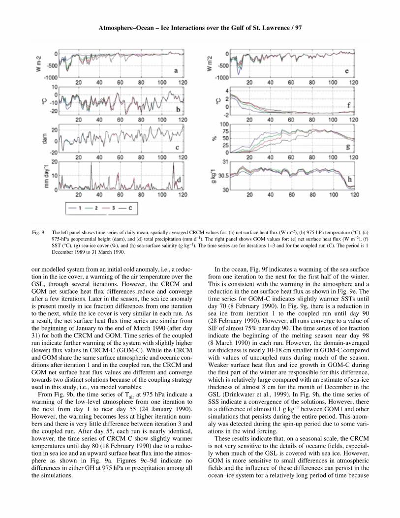
our modelled system from an initial cold anomaly, i.e., a reduc-tion in the ice cover, a warming of the air temperature over theGSL, through several iterations. However, the CRCM andGOM net surface heat flux differences reduce and convergeafter a few iterations. Later in the season, the sea ice anomalyis present mostly in ice fraction differences from one iterationto the next, while the ice cover is very similar in each run. Asa result, the net surface heat flux time series are similar fromthe beginning of January to the end of March 1990 (after day31) for both the CRCM and GOM. Time series of the coupledrun indicate further warming of the system with slightly higher(lower) flux values in CRCM-C (GOM-C). While the CRCMand GOM share the same surface atmospheric and oceanic con-ditions after iteration 1 and in the coupled run, the CRCM andGOM net surface heat flux values are different and convergetowards two distinct solutions because of the coupling strategyused in this study, i.e., via model variables.

From Fig. 9b, the time series of Tair at 975 hPa indicate awarming of the low-level atmosphere from one iteration tothe next from day 1 to near day 55 (24 January 1990).However, the warming becomes less at higher iteration num-bers and there is very little difference between iteration 3 andthe coupled run. After day 55, each run is nearly identical,however, the time series of CRCM-C show slightly warmertemperatures until day 80 (18 February 1990) due to a reduc-tion in sea ice and an upward surface heat flux into the atmos-phere as shown in Fig. 9a. Figures 9c–9d indicate nodifferences in either GH at 975 hPa or precipitation among allthe simulations.

In the ocean, Fig. 9f indicates a warming of the sea surfacefrom one iteration to the next for the first half of the winter.This is consistent with the warming in the atmosphere and areduction in the net surface heat flux as shown in Fig. 9e. Thetime series for GOM-C indicates slightly warmer SSTs untilday 70 (8 February 1990). In Fig. 9g, there is a reduction insea ice from iteration 1 to the coupled run until day 90 (28 February 1990). However, all runs converge to a value ofSIF of almost 75% near day 90. The time series of ice fractionindicate the beginning of the melting season near day 98 (8 March 1990) in each run. However, the domain-averagedice thickness is nearly 10-18 cm smaller in GOM-C comparedwith values of uncoupled runs during much of the season.Weaker surface heat flux and ice growth in GOM-C duringthe first part of the winter are responsible for this difference,which is relatively large compared with an estimate of sea-icethickness of almost 8 cm for the month of December in theGSL (Drinkwater et al., 1999). In Fig. 9h, the time series ofSSS indicate a convergence of the solutions. However, thereis a difference of almost 0.1 g kg–1 between GOM1 and othersimulations that persists during the entire period. This anom-aly was detected during the spin-up period due to some vari-ations in the wind forcing.

These results indicate that, on a seasonal scale, the CRCMis not very sensitive to the details of oceanic fields, especial-ly when much of the GSL is covered with sea ice. However,GOM is more sensitive to small differences in atmosphericfields and the influence of these differences can persist in theocean–ice system for a relatively long period of time because

Atmosphere–Ocean – Ice Interactions over the Gulf of St. Lawrence / 97

Fig. 9 The left panel shows time series of daily mean, spatially averaged CRCM values for: (a) net surface heat flux (W m–2), (b) 975-hPa temperature (°C), (c)975-hPa geopotential height (dam), and (d) total precipitation (mm d–1). The right panel shows GOM values for: (e) net surface heat flux (W m–2), (f)SST (°C), (g) sea-ice cover (%), and (h) sea-surface salinity (g kg–1). The time series are for iterations 1–3 and for the coupled run (C). The period is 1December 1989 to 31 March 1990.

98 / Manon Faucher et al.

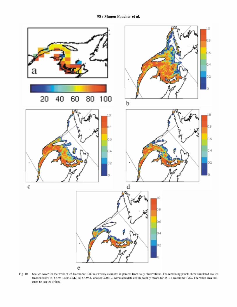
Fig. 10 Sea-ice cover for the week of 25 December 1989 (a) weekly estimates in percent from daily observations. The remaining panels show simulated sea-icefraction from: (b) GOM1, (c) G0M2, (d) GOM3, and (e) GOM-C. Simulated data are the weekly means for 25–31 December 1989. The white area indi-cates no sea ice or land.

of the longer memory of the ocean. The comparison of itera-tion 3 with the coupled run indicates very little (or no) effectof the two-way, daily interaction on atmospheric simulation.However, some effects are shown in ocean–ice simulations.

c Comparison with ObservationsAvailable digitized sea-ice observations are used to evaluatethe effect of the atmosphere–ocean interaction on the oceanicsimulations. In particular, we want to study the evolution ofthe sea-ice field through the iterations from the initial iceanomaly imposed in CRCM1 and make a comparison withthe solution of the coupled run. This section presents a com-parison of the simulated sea-ice covered area for GOM1-3and GOM-C with weekly estimates available from the dailyobserved composites from satellites, aircraft and ship recon-naissance for the week of 25 December 1989. The CanadianIce Service in Ottawa provides these observations with a res-olution of 1° longitude by 1/2° latitude (Fig. 10a). The simu-lated data are weekly averages for the week of 25 December.

Figure 10b indicates that GOM1 overestimates the SIF inthe GSL with much of the area covered with sea ice due tocold atmospheric conditions. In GOM2 (Fig. 10c), thewarmer driving atmosphere gives a reduced SIF comparedwith GOM1, and the ice edge is in the centre of the Gulf, inbetter agreement with observations. However, the sea ice isstill largely overestimated north of Anticosti Island and alongthe north coast. The solution of GOM3 (Fig. 10d) shows fur-ther improvement over the solution of GOM2, especiallynorth of Anticosti Island and along the north coast whereopen water areas are visible. The sea-ice edge is further west,which seems to be in better agreement with observations.These results show the sensitivity of GOM sea-ice cover toatmospheric forcing from the CRCM. The SIF decreased fur-ther from GOM3 to GOM4, especially around AnticostiIsland and east of the Gaspé Peninsula, but remained rela-tively constant in GOM5 and GOM6. The solution of GOM-C is nearly identical to that of GOM6. Figure 10e suggestsless sea ice in GOM-C than the observations. However, it isknown that the observing method tends to overestimate sea-ice cover in the GSL and Fig. 10a represents only an esti-mate of SIF. These results suggest that the model’s solutiontends to return towards observations despite the initial coldcondition imposed in CRCM1.

4 ConclusionThe ocean–ice model for the Gulf of St. Lawrence, GOM andthe CRCM were used in an experiment where they providedthe surface forcing fields to each other. This strategy was usedto test the sensitivity of the CRCM and GOM to each other asa first step towards a fully coupled high-resolution atmos-phere–ocean–ice model for eastern Canada. The main advan-tage of using an exchange of information via the statevariables is the use of the models in their original version.This allows the comparison of our simulations with other sim-ulations which use observations. However, there are some dis-advantages that may affect the results. For example, GOMapproximates the complex atmospheric radiative transfer withrelatively simple formulae typically used in ocean modelling.Furthermore, GOM requires atmospheric variables at the levelof observations, which are not available in the CRCM. The

CRCM variables must be interpolated to the required level forGOM, which introduces uncertainties in the atmospheric forc-ing. These uncertainties might become important becauseGOM appeared to be very sensitive to the atmospheric forcing.

The experiment was performed for a five-month periodfrom 1 November to 31 March 1990, including a spin-up peri-od of one month. In the first part of the experiment both mod-els were used independently and alternately during the studyperiod, but in interaction with an exchange of variablesbetween each run to supply the needed information to theother model for the computation of their own surface fluxes.A series of three iterations was performed with each model toevaluate the sensitivity of the models’ forcing fields to eachother. In the second part of the experiment, a two-way cou-pled simulation was performed by exchanging the variablesevery day for the same period.

The experiment has shown that the GOM, driven by theCRCM atmosphere, is able to provide detailed oceanic sur-face conditions over the GSL that are in relatively goodagreement with its observed state. For example, open waterareas were simulated along the north coast and in the St. Lawrence Estuary due to the offshore winds, while a larg-er SIF was simulated in other areas due to the ridging of theice on the coast. The simulations showed that, on a monthlytimescale, the CRCM is not very sensitive to the changingdistribution of the oceanic forcing fields over the GSL, exceptlocally in the Gulf area and in the atmospheric boundary layerbelow approximately 900 hPa. As a result of an iterative inter-action with the warmer waters of the GOM, the CRCMresponds locally with a slightly lower geopotential heightbelow 900 hPa from CRCM1 to CRCM3, especially in theeastern section of the GSL where relatively large sea-ice dis-tribution differences occur. The low-level temperatureincreases in CRCM2 and CRCM3, producing more diver-gence in the air column, decreasing surface pressure andcyclogenesis at the surface in the GSL area. The solution ofCRCM-C is nearly identical to that of CRCM3, indicatingvery little or no impact of a two-way coupling in atmospher-ic conditions compared with this third uncoupled iteration, ona monthly or longer timescale.

The GOM was shown to be quite sensitive to the differencein atmospheric forcing fields from the CRCM. The warmingof the surface air temperature from one iteration to the nextreduces the net surface atmospheric heat loss in GOM2 andGOM3 over most areas, compared with GOM1, which isreflected in warmer SSTs and reduced sea ice at higher itera-tion numbers. Less sea ice is simulated in the coupled runcompared with uncoupled iterations due to the slightlywarmer surface air and water temperatures. On a seasonaltimescale, the differences in various oceanic fields are lessevident between uncoupled and coupled runs, in response tothe reduced interaction between the CRCM and GOM whenmuch of the GSL is covered with sea ice. However, someanomalies in SIF and in SSS generated in early winter per-sisted until the end of the study period, as well as deeperocean properties. The results suggest that after three iterationsexchanging surface fields between the CRCM and GOM, thesolutions of these models converge towards their respectivesolution, which is in better agreement with observations. Weverified the convergence of the solutions with three additionaliterations for December 1989. We found that a slight warm-

Atmosphere–Ocean – Ice Interactions over the Gulf of St. Lawrence / 99

ing trend continues further into the fourth iteration, which sta-bilizes by the sixth iteration when the solution is nearly iden-tical to the solution of the coupled run. This convergenceindicates that the CRCM and GOM have reached equilibriumwith each other’s forcing.

Stronger winds modify the ocean surface currents and theice motion over much of the area. Interestingly, our experi-ment shows the observed bi-modal structure of the GaspéCurrent, as a result of the interaction between the CRCM andGOM. Our experiment indicates that the position of the GaspéCurrent follows an area of stronger winds, in relation to thesea-ice distribution. In particular, a decrease in sea ice allowsfor further heat exchange between the atmosphere and theocean and a warming of the low-level atmosphere. Thiswarming may be sufficient to destabilize the atmosphericboundary layer off the Gaspé Peninsula and to explain whystronger winds are reaching the surface of the ocean far offthe coast (this problem is under investigation). In CRCM1,the presence of extensive sea ice limits the exchange of heatover the water over much of the area, giving relatively coldsurface temperatures and more stable conditions, which donot allow for stronger winds to develop over Honguedo Strait.

The sensitivity of the CRCM and GOM to each other’sfields was investigated during winter when the atmosphericflow is generally strong. This situation may have decreasedthe impact of the oceanic forcing of the GSL in the CRCMsolution because the travelling systems escape the domainrapidly. This experiment has recently been extended by

Charpentier (2003) to complete one annual cycle and to testthe sensitivity of the models in the summer when the atmos-pheric circulation is usually much weaker. However, theinteractions are generally weaker due to a smaller thermalcontrast between the atmosphere and the ocean, so little sen-sitivity of the CRCM to GOM oceanic fields was found.

In the near future, a river routing scheme will be imple-mented in the physics of the CRCM to link the runoff variableat the river mouths in GOM. This will eliminate the currentuse of runoff data in GOM. The coupling of the CRCM andGOM via the surface fluxes is desirable to ensure a consistentmodelling system and to ensure the conservation of heat,fresh water and momentum across the interface. An in-linecoupling strategy via the surface fluxes is presently beingdeveloped to link the CRCM with regional ocean–ice modelsof the Gulf of St. Lawrence and Hudson Bay. A lake-icemodel for the Great Lakes should also be incorporated in theCRCM in a near future.

AcknowledgmentsWe would like to thank Claude Desrocher and the CRCMresearch group at UQÀM, in particular Michel Giguère fortechnical support. We would also like to thank François Roy,Philippe Gachon, Alain D’astous and André Gosselin atMaurice Lamontagne Institute and Pierre Pellerin atRecherche en prévision numérique (RPN) for their technicalsupport. This work was funded by the Program on EnergyResearch and Development (PERD).

100 / Manon Faucher et al.

ReferencesBESNER, M. 1999. Méthode pour estimer des variables météorologiques horaires

à partir d’observations de navires et de stations terrestres. Rapport scien-tifique, Division des Sciences Atmosphériques et Enjeux Environnementaux,Service météorologique du Canada, Région du Québec, 63 pp.

CAYA, D. 1996. Le modèle régional de climat de l’UQÀM. PhD thesis,Université du Québec à Montréal, Canada, 134 pp. (Available from DanielCaya, département des sciences de la terre et de l’atmosphère, UQÀM).

——— and R. LAPRISE, 1999. A semi-implicit semi-Lagrangian regional cli-mate model: The Canadian RCM. Mon. Weather Rev. 127: 341–362.

CHARPENTIER, D. 2003. Échanges atmosphère-océan entre le Modèle RégionalCanadien du Climat (MRCC) et le Modèle Océanique du Golfe du Saint-Laurent (MOG), M.Sc. thesis, Université du Québec à Montréal, 70 pp.(Available from Dorothée Charpentier, département des sciences de laterre et de l’atmosphère, UQÀM.)

DAVIES, H.C. 1976. A lateral boundary formulation for multi-levels predictionmodels. Q. J. R. Meteorol. Soc. 102: 405–418.

DÖSCHER, R.; U. WILLÉN, C. JONES, A. RUTGERSSON, H.E.M. MEIER, U. HANSSON

and L.P. GRAHAM. 2002. The development of the coupled ocean-atmos-phere model RCAO. Boreal Env. Res. 7(3): 183–192.

DRINKWATER, K.F.; R.G. PETTIPAS, G.L. BUGDEN and P. LANGILLE. 1999. Climaticdata for the northwest Atlantic: A sea ice database for the Gulf of St. Lawrenceand the Scotian Shelf. Can. Tech. Rep. Hydrogr. Ocean. Sci. Vol. 199, 134 pp.

FLATO, G.M. 1994. McPIC: Documentation for the Multi-category Particle-In-Cell Sea Ice model. Can. Tech. Rep. Hydrogr. Ocean. Sci. No. 158,Institute of Ocean Sciences, Sidney, BC, 74 pp.

——— and W.D. HIBLER. 1992. Modeling pack ice as a cavitating fluid.J. Phys. Oceanogr. 22: 626–650.

GACHON, P.; F.J. SAUCIER and R. LAPRISE. 2001. Atmosphere-ocean-ice interactionprocesses in the Gulf of St.Lawrence: numerical study with a coupled model.Presentation at sixth Conference on Polar Meteorology and Oceanographyand the 11th Conference on Interaction of the Sea and Atmosphere, Am.Meteorol. Soc., May 2001, San Diego, California. pp. 14–18.

GATES, W.L. 1992. AMIP: The Atmospheric Model Intercomparison Project,Bull. Am. Meteorol. Soc. 73: 1962–1970.

KOUTITONSKY, V.G. and G.L. BUGDEN. 1991. The physical oceanography of theGulf of St. Lawrence: A review with emphasis on the synoptic variabilityof the motion. In: The Gulf of St. Lawrence: small ocean or big estuary?J.C. Therriault (Ed.), Can. Spec. Pub. Fish. Aquat. Sci., Vol. 113, pp.57–90.

LAPRISE, R.; D. CAYA, M. GIGUERE, G. BERGERON, H. COTE, J.-P. BLANCHET, G.J.BOER and N.A. MCFARLANE S.C. 1998. Climate and climate change in western Canada as simulated by the Canadian Regional Climate Model.ATMOSPHERE-OCEAN, 36(2): 119–167.

LYNCH, A.; W.L. CHAPMAN, J.E. WALSH and G. WELLER. 1995. Development of aregional climate model of the western Arctic. J. Clim. 8: 1555–1570.

MCFARLANE, N.A.; G.J. BOER, J.P. BLANCHET and M. LAZARE. 1992. TheCanadian climate centre second-generation general circulation model andits equilibrium climate. J. Clim. 5: 1013–1044.

MERTZ, G.; V.G. KOUTITONSKY and Y. GRATTON. 1991. On the Seasonal Cycleof the Gaspé Current. In: The Gulf of St. Lawrence: small ocean or bigestuary? J.C. Therriault (Ed.), Can. Spec. Pub. Fish. Aquat. Sci., Vol. 113,pp. 149–152.

PARKINSON, C.L. and W.M. WASHINGTON. 1979. A large-scale numerical modelof sea ice. J. Geophys. Res. 84: 311–337.

ROY, F.; P. PELLERIN, F.J. SAUCIER, J. CHASSÉ and H. RITCHIE. 1999. CoupledAtmosphere-Ice-Ocean Forecasts in the Gulf Of St. Lawrence. In:Preprints 33rd Meeting of the Canadian Meteorological and OceanographicSociety, June 1999, Montreal.

SAUCIER, F.J.; F. ROY, D. GILBERT, P. PELLERIN and H. RITCHIE. 2003a. The for-mation of water masses and sea ice in the Gulf of St. Lawrence. J. Geophys.Res. 108 (C8): 3269–3289.

———; s. SNNEVILLE, S. PRINSENBERG, F. ROY, P. GACHON, D. CAYA and R.LAPRISE. 2003b. Modeling the Ice-Ocean Seasonal Cycle in Hudson Bay,Foxe Basin and Hudson Strait, Canada. Clim. Dyn. in press.

SMAGORINSKY, J. 1963. General circulation experiment with primitive equa-tions. I. The basic experiment. Mon. Weather Rev. 91(3): 99–164.