J Optim Theory ApplDOI 10.1007/s10957-013-0439-9

Sensitivity Analysis of Merit Function in SolvingNonlinear Equations by Optimization

Seyyed Shahabeddin Azimi · Mansour Kalbasi ·Hamidreza Sadeghifar

Received: 12 April 2013 / Accepted: 25 September 2013© Springer Science+Business Media New York 2013

Abstract To solve nonlinear equations by an optimization method, scaling is veryimportant. Two types of poor scaling where: (a) the variables differ greatly in magni-tude; (b) the merit function of system is highly sensitive to small changes in certainvariables and relatively insensitive to changes in other variables. If poor scaling isignored, the algorithm may produce solutions with poor quality. To solve (a), we canchange units of variables. A numerical solution of the nonlinear equations producedby the finite volume method in the forced convective heat transfer of a nanofluid, as acase study, indicates that the poor scaling (b) is solved by using the Euclidean normof columns of the Jacobian matrix as scaling data, while some researchers proposeddiagonal elements of the Hessian matrix as scaling data.

Keywords Nonlinear equations · Optimization · Merit function · Scaling matrix ·Jacobian

1 Introduction

In many applications, it is required to solve nonlinear equations. Some importantiterative methods for solving nonlinear equations are designed on the basis of opti-mization.

An important matter in the optimization is scaling. Ordinary poor scaling is oc-curring where, for example, some of the unknowns have values of about 105 (e.g.,

S.S. Azimi · M. Kalbasi (B)Department of Chemical Engineering, Amirkabir University of Technology, Hafez Avenue, Tehran,Irane-mail: mkalbasi@aut.ac.ir

H. SadeghifarSchool of Mechatronic Systems Engineering, Simon Fraser University, Surrey V3T 0A3,British Columbia, Canada

J Optim Theory Appl

the pressure in nanofluid problems), while the others have the order of 10−2 (e.g.,the nanoparticle volume fraction in nanofluid problems). If such wide variations areignored, the algorithm may encounter numerical difficulties or produce solutions ofpoor quality [1]. The remedy is either to scale the unknowns or to change their units.

The scaling explained above is a primitive one, while optimization problems areoften posed with another poor scaling where the merit function is highly sensitive tosmall changes in certain variables and relatively insensitive to changes in others [1].

This work is concerned with the second type of poor scaling in solving nonlinearequations of the forced concoctive heat transfer of nanofluid and is structured as fol-lows. The optimization method is briefly described in Sect. 2.1. Nonlinear equationsare introduced in Sect. 2.2. In Sect. 3, repairing the second type of poor scaling isdiscussed based on the simulation results. Finally, a summary of the conclusions isgiven in Sect. 4.

2 Theory

2.1 Optimization

Consider a nonlinear equation as

F(x) = 0, (1)

where F : Rn → Rn is the vector of functions (residual vector), Fi(x) : Rn → R and

x is the vector of variables. To solve this nonlinear system by optimization, a meritfunction is defined, which is a scalar-valued function of x, whose value indicateswhether a new vector x is better or worse than the current one, in the sense of makingprogress toward a root of F [1]:

f (x) = 1

2

∥∥F(x)

∥∥

2 = 1

2

n∑

i=1

F 2i . (2)

Here, the problem of solving the nonlinear equations (F(x) = 0) is transformedinto the problem of minimizing a merit function (minimizing f (x)).

As mentioned before, an important matter in the optimization is scaling. Poorlyscaled functions arise, for example, in simulations of physical and chemical systemswhere different processes are taking place at very different rates [1]. Ordinary poorscaling can be solved by changing units of unknowns. The following expression ex-plains this remedy:

x = Ux →

⎡

⎢⎢⎢⎣

φ

T

p

uz

⎤

⎥⎥⎥⎦

=

⎡

⎢⎢⎢⎣

10−2 0 0 0

0 102 0 0

0 0 105 0

0 0 0 10−2

⎤

⎥⎥⎥⎦

⎡

⎢⎢⎢⎣

φ

T

p

uz

⎤

⎥⎥⎥⎦

,

o(φ) � 10−2 o(T ) � 102 o(p) � 105 o(uz) � 10−2,

(3)

J Optim Theory Appl

where o( ) denotes the order of magnitude, φ is the nanoparticle volume fraction, T isthe nanofluid temperature, uz is the axial velocity of the nanofluid, p is the nanofluidpressure, and U is a diagonal matrix with positive elements which are equal to theorder of magnitude of the unknowns in the SI units [2]. The above variables are withinthe scope of the forced convective heat transfer of nanofluids.

To give an example for the second type of poor scaling, the following merit func-tion can be considered:

g(x) = 109x21 + 2x2

2 , (4)

where, clearly, g(x) is very sensitive to even small changes in x1 but not to perturba-tions in x2.

One of the important methods for solving Eq. (1) as an optimization method is theLevenberg–Marquardt (LM) method:

(

J T J + λD)

S = −J T F X(new) = X(current) + S J =

⎡

⎢⎢⎣

∂F1∂x1

· · · ∂F1∂xn

......

∂Fn

∂x1· · · ∂Fn

∂xn

⎤

⎥⎥⎦

,

(5)where S is the step, J is the Jacobian of F , J T is the transpose of J , λ is a positivedamping factor, and D is a diagonal matrix with positive elements which repairs thispoor scaling, e.g., Eq. (4). As f (x) is highly sensitive to the value of a componentof x, the corresponding diagonal element of D is set to be large and vice versa.

The choice of matrix D is very important, which is studied here with regard tothe forced convective heat transfer of nanofluid in which the temperature profile isrequired for analyzing heat transfer improvement.

It was proposed that information to construct the scaling matrix D can be derived

from the second derivatives ∂2f

∂x2i

. In other words, the scaling matrix D is equal to the

diagonal elements of the Hessian (∇2f ) or an approximation of it (J T J ) [1]:

D(i, i) = H(i, i) =(

∂2f

∂x2i

)

≈ J T J (i, i). (6)

2.2 Defining an Application as Case Study (Nonlinear Equations)

Heat transfer plays an important role in many fields such as power generation, airconditioning, transportation, and microelectronics due to the heating and coolingprocesses involved [3]. Nanofluids, fluids with nanoparticles suspended in them, canbe considered to be the next-generation heat transfer fluids as they offer excitingnew possibilities to enhance heat transfer performance compared to pure liquids [4].The heat transfer coefficient is the determining factor in forced convection cooling–heating applications of heat exchange equipments including engines and engine sys-tems [5]. To obtain the heat transfer coefficient, the temperature profile is required.

To obtain the temperature profile of a nanofluid in the forced convective heat trans-fer in the developing laminar flow inside a horizontal tube (see Fig. 1), the followingdifferential equations (conservation laws) must be solved.

J Optim Theory Appl

Fig. 1 A horizontal tube

Mass conservation of nanofluid:

1

r

∂(rρnf ur)

∂r+ ∂(ρnf uz)

∂z= 0. (7a)

Mass conservation of nanoparticle:

1

r

∂(rφρnf ur)

∂r+ ∂(φρnf uz)

∂z+ 1

r

∂(rjpr )

∂r+ ∂(jpz)

∂z= 0. (7b)

Momentum conservation in the radial direction:

ρnf

(

ur

∂ur

∂r+ uz

∂ur

∂z

)

= −∂p

∂r− 1

r

∂(rτrr )

∂r− ∂τzr

∂z+ τθθ

r+ ρnf gr . (7c)

Momentum conservation in the axial direction:

ρnf

(

ur

∂uz

∂r+ uz

∂uz

∂z

)

= −∂p

∂z− ∂τzz

∂z− 1

r

∂(rτrz)

∂r. (7d)

Energy conservation of nanofluid:

1

r

∂

∂r

(

rur(ρcp)nf T) + ∂

∂z

(

uz(ρcp)nf T)

+[

1

r

∂

∂r

(

−rknf

∂T

∂r

)

+ ∂

∂z

(

−knf

∂T

∂z

)]

= 0. (7e)

These differential equations are transformed to the algebraic equations, discretizedequations, by the finite volume method. In this method, the domain (tube) is dividedinto non-overlapping control volumes in which one nodal point is placed in the centerof each control volume. The control volume in this application has a ring shape.By integration of differential equations over a control volume and applying Gauss’divergence theorem, the discretized equations are obtained [6–8].

If V is a closed region in space enclosed by a surface Y , the Gauss divergencetheorem is defined as

∫

V

(∇.Q)dV =∫

Y

(n.Q)dY, (8)

in which n is the outwardly directed unit normal vector and Q is a vector (or tensor).The discretized form of Eq. (7a) is

(ρnf uzA)e − (ρnf uzA)w + (ρnf urA)n − (ρnf urA)s = 0, (9)

J Optim Theory Appl

Fig. 2 Two-dimensionalillustration of the application(horizontal tube)

where A is the cross-sectional area of the control volume face, ρnf is the density ofthe nanofluid, uz is the nanofluid axial velocity, ur is the nanofluid radial velocity andthe subscripts e, w, n, and s denote the face directions, see Fig. 2. West (w) is the facesuch that the outwardly directed normal vector to it is in the (−δz) direction (δ is theunit vector in the cylindrical coordinates). East (e) is the face such that the outwardlydirected normal vector to it is in the (δz) direction. South (s) is the face such that theoutwardly directed normal vector to it is in the (−δr ) direction. North (n) is the facesuch that the outwardly directed normal vector to it, is in the (δr ) direction.

The discretized form of Eq. (7b) is

(φρpuzA)e − (φρpuzA)w + (φρpurA)n − (φρpurA)s + (jzA)e

− (jzA)w + (jrA)n − (jrA)s = 0, (10)

where φ is the volume fraction of nanoparticle, ρp is the density of nanoparticle, jr

is the nanofluid mass rate due to the diffusion in the radial direction, and jz is thenanofluid mass rate due to the diffusion in the axial directions. It can be shown thatthe diffusion terms can be neglected.

The discretized form of Eq. (7c) is

(ρnf uruzA)e − (ρnf uruzA)w + (ρnf ururA)n − (ρnf ururA)s + pnode − ps

drV

+ (

(τzrA)e − (τzrA)w + (τrrA)n − (τrrA)s) − (

ρnf (−g))

V = 0, (11)

where p is the nanofluid pressure, g is the gravitational acceleration, τ is the shearstress tensor (subscripts of τ denote components of shear stress), V is the volume, ofcontrol volume and dr is node spacing in the radial direction.

The discretized form of Eq. (7d) is

(ρnf uzuzA)e − (ρnf uzuzA)w + (ρnf uzurA)n − (ρnf uzurA)s + pnode − pw

dzV

+ (

(τzzA)e − (τzzA)w + (τrzA)n − (τrzA)s) = 0, (12)

where dz is the node spacing in the axial direction.

J Optim Theory Appl

The discretized form of Eq. (7e) is

(

uz(ρcp)nf T A)

e − (

uz(ρcp)nf T A)

w + (

ur(ρcp)nf T A)

n − (

ur(ρcp)nf T A)

s

−(

knf

∂T

∂zA

)

e+

(

knf

∂T

∂zA

)

w−

(

knf

∂T

∂rA

)

n+

(

knf

∂T

∂rA

)

s= 0,

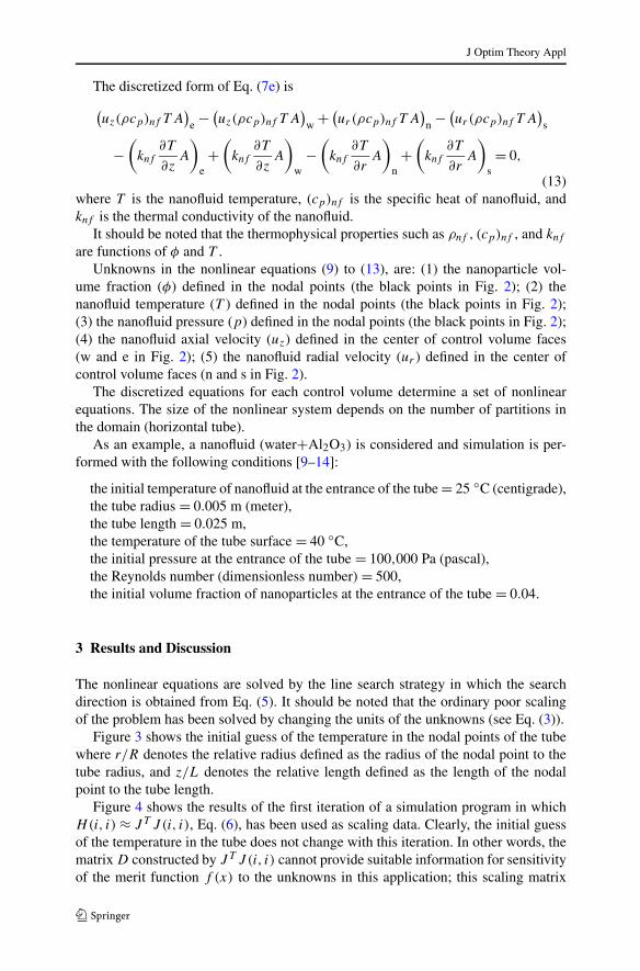
(13)where T is the nanofluid temperature, (cp)nf is the specific heat of nanofluid, andknf is the thermal conductivity of the nanofluid.

It should be noted that the thermophysical properties such as ρnf , (cp)nf , and knf

are functions of φ and T .Unknowns in the nonlinear equations (9) to (13), are: (1) the nanoparticle vol-

ume fraction (φ) defined in the nodal points (the black points in Fig. 2); (2) thenanofluid temperature (T ) defined in the nodal points (the black points in Fig. 2);(3) the nanofluid pressure (p) defined in the nodal points (the black points in Fig. 2);(4) the nanofluid axial velocity (uz) defined in the center of control volume faces(w and e in Fig. 2); (5) the nanofluid radial velocity (ur ) defined in the center ofcontrol volume faces (n and s in Fig. 2).

The discretized equations for each control volume determine a set of nonlinearequations. The size of the nonlinear system depends on the number of partitions inthe domain (horizontal tube).

As an example, a nanofluid (water+Al2O3) is considered and simulation is per-formed with the following conditions [9–14]:

the initial temperature of nanofluid at the entrance of the tube = 25 ◦C (centigrade),the tube radius = 0.005 m (meter),the tube length = 0.025 m,the temperature of the tube surface = 40 ◦C,the initial pressure at the entrance of the tube = 100,000 Pa (pascal),the Reynolds number (dimensionless number) = 500,the initial volume fraction of nanoparticles at the entrance of the tube = 0.04.

3 Results and Discussion

The nonlinear equations are solved by the line search strategy in which the searchdirection is obtained from Eq. (5). It should be noted that the ordinary poor scalingof the problem has been solved by changing the units of the unknowns (see Eq. (3)).

Figure 3 shows the initial guess of the temperature in the nodal points of the tubewhere r/R denotes the relative radius defined as the radius of the nodal point to thetube radius, and z/L denotes the relative length defined as the length of the nodalpoint to the tube length.

Figure 4 shows the results of the first iteration of a simulation program in whichH(i, i) ≈ J T J (i, i), Eq. (6), has been used as scaling data. Clearly, the initial guessof the temperature in the tube does not change with this iteration. In other words, thematrix D constructed by J T J (i, i) cannot provide suitable information for sensitivityof the merit function f (x) to the unknowns in this application; this scaling matrix

J Optim Theory Appl

Fig. 3 Initial guess of thetemperature

Fig. 4 Simulation results due to

JT J (i, i) as scaling data;Iteration = 1

determines a search direction (vector S) which has low quality, i.e., vector x stops atthe initial guess.

Each element of matrix J T J is equal to the multiplication of two columns ofJacobian. Therefore, the diagonal elements of matrix J T J are obtained as

J T J (i, i) =(

∂F1

∂xi

)2

+ · · · +(

∂Fn

∂xi

)2

. (14)

Table 1, for example, gives some values of the diagonal elements of matrix J T J inwhich different scaling values have been calculated because the variables are differentin nature. Each variable in the discretized equations has different coefficients and thusdifferent values are obtained in the computation of the Jacobian elements (

∂Fi

∂xk).

Coefficients due to the nanofluid pressure are:

Eq. (11) → Coefficient = Scale(p)V

dr∼ 1,

O(

Scale(p)) ∼ 105 O(vol) ∼ 10−8 O(dr) ∼ 10−3,

Eq. (12) Coefficient = Scale(p)V

dz∼ 1,

O(dz) ∼ 10−3,

J Optim Theory Appl

Table 1 Scaling values due tothe matrix JT J Values of JT J (i, i) Variable

0.0122104 Nanoparticle volume fraction

0.114903

0.709246

0.884566 Nanofluid temperature

8.19208

82.3783

0.434879 Nanofluid pressure

3.46978

15.8731

0.000356725 Nanofluid axial velocity

0.0128104

0.00926973

where Scale(p) denotes the order of magnitude of pressure. Some coefficients due tothe nanofluid temperature are:

Eq. (11) → Coefficients ={

Scale(uz)urScale(uz)uz(1 − Scale(φ)φ)Aw ∼ 10−12

Scale(uz)urScale(uz)ur(1 − Scale(φ)φ)As ∼ 10−15,

ρnf = φρp + (1 − φ)ρf →{

ρf = function of T

ρp = constant,

O(As) ∼ 10−5 O(Aw) ∼ 10−5 O(

Scale(uz)) ∼ 10−2,

O(

Scale(φ)) ∼ 10−2 O(φ) ∼ 1 O(uz) ∼ 1 O(ur) ∼ 10−3,

Eq. (12) → Coefficients ={

Scale(uz)uzScale(uz)uz(1 − Scale(φ)φ)Aw ∼ 10−9

Scale(uz)urScale(uz)uz(1 − Scale(φ)φ)As ∼ 10−12,

Eq. (13) → Coefficients =

⎧

⎪⎪⎪⎪⎪⎪⎨

⎪⎪⎪⎪⎪⎪⎩

Scale(uz) uz︸︷︷︸

new(uz)

(ρcp)nf Aw ∼ 10−1

Scale(uz)ur(ρcp)nf As ∼ 10−4

knfAw

dz∼ 10−3

knfAs

dr∼ 10−3,

O(knf ) ∼ 10−1 O(ρcp)nf ∼ 6 × 106,

where Scale(uz) is the order of magnitude of the nanofluid axial velocity andScale(φ) is the order of magnitude of the nanoparticle volume fraction. Some co-

J Optim Theory Appl

efficients due to the nanoparticle volume fraction are:

Eq. (9) → Coefficients ={

Scale(uz)uzScale(φ)ρpAw ∼ 10−5

Scale(uz)urScale(φ)ρpAs ∼ 10−6,

O(ρp) ∼ 104,

Eq. (11) → Coefficients ={

Scale(uz)urScale(uz)uz(ρp − ρf )Aw ∼ 10−8

Scale(uz)urScale(uz)ur(ρp − ρf )As ∼ 10−11,

O(ρf ) ∼ 103,

Eq. (12) → Coefficients ={

Scale(uz)uzScale(uz)uz(ρp − ρf )Aw ∼ 10−5

Scale(uz)urScale(uz)uz(ρp − ρf )As ∼ 10−8.

Some coefficients due to the nanofluid axial velocity are:

Eq. (9) → Coefficients = Scale(uz)Scale(φ)φρpAw ∼ 10−5,

Eq. (10) → Coefficients = Scale(uz)Scale(uz)ρnf urAw ∼ 10−9,

Eq. (11) → Coefficients = Scale(uz)Scale(uz)ρnf uzAw ∼ 10−6,

Eq. (12) → Coefficients = Scale(uz)T (ρcp)nf Aw ∼ 10,

O(T ) ∼ 102.

As mentioned above, these scaling values cannot provide a suitable search di-rection for solving nonlinear equations. It seems that where all absolute values of acolumn of the Jacobian are smaller than 1, the corresponding diagonal element ofJ T J may underestimate the scaling value since squaring is done with real numberswhich are smaller than 1 (e.g., values due to the nanofluid axial velocity in Table 1).On the other hand, where some components of a column of the Jacobian have ab-solute values which are larger than 1, the corresponding diagonal element of J T J

may overestimate the scaling value (e.g., values due to the nanofluid temperature inTable 1).

To solve this problem, we can consider each column of the Jacobian as a vectorand define the matrix D as Euclidean norm of these columns:

D(i, i) = normJ (i) =√

(∂F1

∂xi

)2

+ · · · +(

∂Fn

∂xi

)2

. (15)

By this method, the components of the scaling matrix D can be computed by thenorm of each column of Jacobian. Table 2 gives the corresponding values of Table 1due to the norm J .

Figure 5 shows the first iteration of the simulation program in which the norm J ,Eq. (15), is used as scaling data. This scaling matrix determines a search directionwhich has high quality. With analysis of results in the next iterations, it can be con-cluded that the main change in the initial guess occurs in the first iteration, in otherwords, the first iteration takes a long step to the solution.

J Optim Theory Appl

Table 2 Scaling values due tothe norm J Some values of norm J Variable

0.110501 Nanoparticle volume fraction

0.338974

0.842168

0.940514 Nanofluid temperature

2.86218

9.07625

0.659454 Nanofluid pressure

1.86274

3.98411

0.0188872 Nanofluid axial velocity

0.113183

0.0962795

Fig. 5 Simulation results due tonorm J as scaling data;Iteration = 1

The numerical simulation is validated against the available results of the followingequation [15]:

uzρcp

∂T

∂z− k

[1

r

∂

∂r

(

r∂T

∂r

)]

= 0. (16)

Equation (16) describes the forced convective heat transfer of a pure fluid with con-stant thermophysical properties in the fully developed laminar region of a circulartube. Figure 6 shows the local Nusselt number of both analytical solution and ournumerical results, where z is the axial coordinate, R is the tube radius, and Pr and Rein Fig. 6 denote the Prandtl number and the Reynolds number, respectively, used inthe study of convective heat transfer.

To solve poor scaling (b), the following propositions are suggested: (1) chang-ing the coefficients of variables to have the same order of magnitude; this methodis critical since it may increase the poor scaling by changing other coefficients inan equation; (2) obtaining some variables as a function of other variables or remov-ing some variables and equations; this method is done by analyzing equations andparticularly the geometry of problem.

J Optim Theory Appl

Fig. 6 Local Nusselt number ofboth analytical solution andnumerical simulation

4 Conclusions

The simulation results of this application indicate that the scaling matrix due to thesecond type of poor scaling should be calculated by the norm of columns of Jacobianmatrix. The coefficients of the variables in nonlinear equations play an important rolein the degree of poor scaling; and it is possible to reduce the poor scaling by changingthese coefficients.

References

1. Nocedal, J., Wright, S.J.: Numerical Optimization. Springer, New York (1999)2. Dennis, J.E., Schnabel, R.B.: Numerical Methods for Unconstrained Optimization and Nonlinear

Equations. Classics in Applied Mathematics. SIAM, Philadelphia (1987)3. Özerinç, S., Kakaç, S., Yazıcıoglu, A.G.: Enhanced thermal conductivity of nanofluids: a state-of-the-

art review. Microfluid. Nanofluid. 8, 145–170 (2010)4. Wang, X., Mujumdar, A.S.: Heat transfer characteristics of nanofluids: a review. Int. J. Therm. Sci.

46, 1–19 (2007)5. Kakaç, S., Pramuanjaroenkij, A.: Review of convective heat transfer enhancement with nanofluids.

Int. J. Heat Mass Transf. 52, 3187–3196 (2009)6. Ferziger, J.H., Peric, M.: Computational Methods for Fluid Dynamics. Springer, Berlin (2002)7. Versteeg, H.K., Malalasekera, W.: An Introduction to Computational Fluid Dynamics the Finite Vol-

ume Method. Longman Scientific & Technical, Harlow (1995)8. Bird, R.B., Stewart, W.E., Lightfoot, E.N.: Transport Phenomena, Wiley, New York (2007)9. Brady, J.F., Khair, A.S., Swaroop, M.: On the bulk viscosity of suspensions. J. Fluid Mech. 554,

109–123 (2006)10. Zhou, S.Q., Ni, R.: Measurement of the specific heat capacity of water-based Al2O3 nanofluid. Appl.

Phys. Lett. 92(9), 0931231 (2008)11. Kanzow, C., Yamashita, N., Fukushima, M.: Levenberg–Marquardt methods for constrained nonlinear

equations with strong local convergence properties. J. Comput. Appl. Math. 172, 375–397 (2004)12. Nguyen, C.T., Desgranges, F., Galanis, N., Roya, G., Maréd, T., Boucher, S., Angue Mintsa, H.:

Viscosity data for Al2O3–water nanofluid—hysteresis: is heat transfer enhancement using nanofluidsreliable? Int. J. Therm. Sci. 47, 103–111 (2008)

13. Li Calvin, H., Peterson, G.P.: Experimental investigation of temperature and volume fraction varia-tions on the effective thermal conductivity of nanoparticle suspensions (nanofluids). J. Appl. Phys.99, 084314 (2006)

14. Pathipakka, G., Sivashanmugam, P.: Heat transfer behaviour of nanofluids in a uniformly heated cir-cular tube fitted with helical inserts in laminar flow. Superlattices Microstruct. 47, 349–360 (2010)

15. Kays, W.M., Crawford, M.E.: Convective Heat and Mass Transfer. McGraw-Hill, New York (1993)