Embed Size (px)
Citation preview

Sensitivity Analysis of Convection of the 24 May 2002 IHOP Case Using Very Large
Ensembles
William J. Martin1* and Ming Xue1,2
1Center for Analysis and Prediction of Storms, Norman, Oklahoma
1,2School of Meteorology, Norman, Oklahoma
Submitted to Monthly Weather Review
September, 2004
*Corresponding author address:
Dr. William Martin
Center for Analysis and Prediction of Storms
100 East Boyd, SEC Room 1110
Norman, OK 73019.
Phone: (405) 325-0402
E-mail: [email protected]

2
ABSTRACT
This paper introduces the use of very large ensembles for detailed sensitivity analysis and
applies this technique to study the sensitivity of model forecast rainfall to initial boundary-layer
and soil moisture fields for a particular case from the IHOP-2002 field program. In total, an
aggregate ensemble of over 12 000 mesoscale model forecasts are made, with each forecast
having different perturbations of boundary layer moisture, boundary layer wind, or soil moisture.
Sensitivity fields are constructed from this ensemble, producing detailed sensitivity fields of
defined forecast functions to initial perturbations. This work is based on mesoscale model
forecasts of convection of the 24 May 2002 IHOP case, which saw convective initiation along a
dryline in western Texas as well as precipitation along a cold front. The large ensemble
technique proves to be highly sensitive, and both significant and subtle connections between
model state variables are revealed. A number of interesting sensitivity results is obtained. It is
found that soil moisture and ABL moisture have opposite effects on the amount of precipitation
along the dryline; that moisture on both the dry and moist sides of the dryline were equally
important; and that some small perturbations were alone responsible for entire convective storm
cells near the cold front, a result implying a high level of nonlinearity. These sensitivity analyses
strongly indicate the importance of accurate low-level water vapor characterization for
quantitative precipitation forecasting.

3
1. Introduction
One goal of the IHOP project (13 May through 25 June 2002; Weckwerth et al., 2004) is
to improve the prediction of convection and the associated precipitation through improved low-
level water vapor characterization. This paper attempts to address this issue by analyzing the
sensitivity of a model forecast for an IHOP case (the 24 May 2002 convective initiation case) to
small perturbations in the atmospheric boundary layer (ABL) fields and surface moisture at the
initial model time. This is accomplished by testing a large set of possible initial ABL
perturbations to fields of water vapor mixing ratio (qv), volumetric soil moisture content (qs), and
meridional wind component (v). The number of initial perturbations tested is large (2016 for
each variable), requiring a large number of forward model runs, which could only be
accomplished in a reasonable amount of time by using a large parallel computing system. From
these sets of perturbed runs, detailed sensitivity fields are constructed. The model used is the
Advanced Regional Prediction System (ARPS, Xue et al., 2000, 2001, 2003), a multi-scale
nonhydrostatic atmospheric modeling system.
The sensitivity fields constructed in the paper are analogous to those produced by adjoint
models (Kim et al., 2004; Kleist and Morgan, 2002; Errico and Vukicevic, 1992; Errico, 1997;
Hall et al., 1982, Hall and Cacuci, 1983). However, adjoint methods are difficult to implement
for complex models, especially those employing complex physical parameterizations (Errico,
2003). Also, because adjoints are linear models, adjoint-derived sensitivities can fail to be
meaningful if long time integrations are involved where non-linearities in the model become
important. For these reasons, explorations of forecast sensitivities have sometimes taken the
approach of using a number of direct model integrations (e.g., Crook, 1996; Mullen and
Baumhefner, 1994). Due to limitations in computational power, these sensitivity analyses from

4
forward model runs have necessarily been limited to a small number (10 to 100) of model runs.
Sensitivity fields are useful for understanding predictability, for understanding physical
connections between variables, and for use in data assimilation where model initial fields are
adjusted using forecast sensitivities.
The availability of large parallel computer systems with thousands of processors now makes
it possible to obtain sensitivity fields from a very large number (thousands) of nonlinear forward
model runs with full physics, with each model run having a small perturbation at a different
location in space. Small, spaced perturbations at a large number of locations can be used, and
sensitivity fields can be constructed from such very large ensembles (VLE) of model runs. The
number of perturbations necessary to characterize the entire three-dimensional model space is
proportional to the number of degrees of freedom in the model, i.e., the number of input
variables times the number of grid points. This would still be too many perturbed model runs to
make for even for the most powerful of modern super-computers. Consequently, this method is
only viable for calculating two-dimensional sensitivity fields. An exploration of the sensitivity
of a forecast to (two-dimensional) atmospheric boundary layer (ABL) fields and surface soil
model fields is an appropriate application of the VLE technique.
It is important to note the similarities and differences between the VLE technique and the
adjoint technique. They both calculate the same dimensional sensitivity of a defined response
function of a forecast, J (which might be, for example, the total rainfall in some area), to an
initial model state variable, a0 (where a0 might be the initial field of ABL moisture), 0a
J∂∂ . To
calculate 0a
J∂∂ , the VLE technique use a small perturbation in a0 and calculates the change in J
by calculating the difference between the perturbed and unperturbed runs. The adjoint method

5
uses the actual mathematical derivative of the model and directly calculates 0a
J∂∂ (essentially
through many recursive applications of the chain rule for differentiation). The adjoint, therefore,
gives the exact sensitivity for infinitesimal perturbations; while the VLE technique gives the
actual sensitivity for a finite perturbation. If the perturbation size used in the VLE technique is
sufficiently small, then the two techniques, in principle, give the same result. Nonlinearity of the
model, however, can lead to different results even for relatively small perturbations. There is
also a minimum to the size of the perturbations that can be used in the VLE technique because of
round-off error.
For the rest of this paper, section 2 introduces briefly the case, the ARPS model and its
configuration used for the forecast, and provides the details of the VLE technique. The results
are presented in section 3, and a summary is given in section 4, together with additional
discussion.
2. ARPS model and the VLE technique
a. The 24 May 2002 case, ARPS configuration, and the initial condition
A forecast was made from initial fields at 1800 UTC on 24 May 2002. This is local noon for
the study area in the southern Great Plains of the United States. The initial fields were obtained
by interpolation from the 40-km resolution ETA analysis at 1800 UTC. The interpolation was
done to a 135x135x53 (x, y, z, respectively) grid with a 9 km horizontal grid spacing, centered
over the IHOP study area in the southern Great Plains. The model used a vertically stretched
grid with a minimum spacing at the surface of 20 m, and a maximum height of about 20 km.
The first level above the ground was, therefore, at 10 m above the ground. The time step size

6
was 15 seconds. Figure 1 shows the initial surface (about 10 m elevation) fields of water vapor
and wind vector.
We employed the ARPS model using leap-frog time differencing, fourth-order centered
advection in both the horizontal and vertical directions, and a mode-split with vertically implicit
treatment for acoustic waves. Fourth-order computational mixing is included to suppress small-
scale noise and a 6 km thick Rayleigh damping layer is applied near the upper boundary. The
lateral boundaries are forced by boundary conditions obtained from temporal and spatial
interpolations of the 18 UTC 40-km horizontal-resolution ETA forecast at 3 hour intervals.
The ARPS model contains many physical parameterization schemes which can give a high
degree of physical realism to forecasts. For this work, we used the following physical
parameterizations: full ice microphysics including cloud, rain, ice, snow, and hail variables; a
complex long and short-wave radiation transfer parameterization; stability-dependent surface
fluxes; a two-layer force-restore type soil-vegetation model including soil moisture and soil
temperature as prognostic variables, a non-local TKE-based PBL parameterization scheme, a
1.5-order TKE-based subgrid-scale turbulence model; and detailed terrain and land-surface
characteristics definitions. The two-layer soil model includes a surface layer and a one meter
deep soil layer. The soil and vegetation types and other land surface characteristics were derived
from a 1 km data base; in addition, three soil types were defined for each grid cell, each carrying
a percentage weighting derived from the data. More details on the model and physical
parameterizations can be found in the ARPS description papers (Xue et al., 2000, 2001, 2003).
Convective and cumulus parameterization schemes are available in ARPS, but were not used
for this study even though, with a 9 km horizontal resolution, the model is not expected to be
able to represent convective cells with complete realism. Convective parameterization has

7
limitations as well, and preliminary forecast runs of this case with explicit convection appeared
more realistic and agreed better with the observed fields than runs using convective
parameterization. Consequently, the decision was made not to include convective
parameterization. The results of the unperturbed control run are qualitatively similar to the 3 km
and 1 km resolution simulations of the same case done by Xue and Martin (2004).
All forward model runs were made for six hours from the 1800 UTC 24 May initial condition
to 0000 UTC 25 May. The unperturbed model forecast fields of 10 meter water vapor and wind
vectors are shown in Fig. 2. Fig. 3a shows the vertically integrated liquid water field at the
forecast time and Fig. 3b shows the total accumulated rainfall through six hours.
While an attempt at a high degree of agreement with the observed convection was not made,
this forecast is similar in many respects to the actual weather on 24 May 2002. The observations
are described in great detail elsewhere (e.g., Wakimoto et al., 2004; Holt et al., 2004; Xue and
Martin, 2004) and will not be repeated in detail here. Figure 1 shows the general situation at
1800 UTC before any convection has occurred. A dryline was oriented north-south from the
central eastern Texas panhandle southward, and a cold front existed from the central eastern
Texas panhandle northeastward through eastern Kansas. A triple point low existed at the
intersection of the dryline and cold front. After six hours in the real atmosphere, the triple point
had moved southeastward and convection initiated at about 2030 UTC in northwest Texas south
of the triple point. The ARPS forecast presented here in Figs. 2-3 captured the location of
convective initiation along the dryline accurately, although it initiated convection later than
observed, and by 0000 UTC 25 May, much less convection occurred in the model than in the
actual atmosphere. Also, the model has more rain near the cold front in northwestern Oklahoma
than was observed. Despite particular differences between the model forecast and the

8
observations, useful sensitivity analyses of details of convection along the cold front and dryline
in the model forecast can be made.
b. The very large ensemble technique
To calculate the sensitivity field of the model forecast to the initial fields, we use an
exhaustive range of perturbed forward model runs. In each run, a perturbation of one initial field
variable in a different location is made. The backwards in time sensitivity field is then
assembled from this ensemble of forward model runs. Considering just a 135x135x53 grid with
potentially six primitive variables that one might be interested in perturbing (three wind
components, pressure, temperature, and water vapor), there are 5 795 550 possible ways a single
perturbation could be added to the initial condition to test its impact. It is also possible to vary
the size of the perturbation, leading to a further multiplication of potential perturbations to
examine. It is not practical to try this many perturbations with current computers. To reduce this
number to one practically manageable, we selected to perturb only certain variables in a two–
dimensional surface layer. We chose to make the perturbations 27 km by 27 km in horizontal
size (3 grid cells by 3 grid cells) and 1 km in vertical depth at the surface (or 1 m in depth for soil
moisture). The horizontal domain can be completely covered by placing perturbations of this
size onto 2025 different horizontal places on the grid at the initial time. The 1 km depth for the
perturbation is chosen because it approximates the depth of the ABL for this case at the initial
time. We only perturbed water vapor mixing ratio, qv (which affects the convective available
energy and precipitable water), volumetric soil moisture, qs (which affects latent and sensible
heat fluxes into the atmosphere), and meridional wind, v (which affects northward transport of
moisture and wind shear) as it is believed that these are the variables that have the greatest
impact on precipitation. For the qs perturbations, both the surface and deep layers were given the

9
same perturbation. To investigate the possibility of nonlinear sensitivity effects, each variable is
perturbed with both positive and negative perturbations. In principle, if the sensitivity fields
depend linearly on the size of the initial perturbations, then identical results should be obtained
by using positive and negative perturbations.
The size of the perturbation must be large enough so that round-off errors in model
calculations do not overwhelm the effects of the perturbations. They must also be small enough
so that the perturbed model forecast is reasonable. For example, if too large an ABL moisture
perturbation were used, condensation in the model would immediately be triggered at the
perturbation site, leading to a model forecast quite different from the unperturbed forecast and
one which would never have happened with any reasonable-size error in the initial condition.
From preliminary tests, it was found that perturbations of about 10% of the magnitude of the
unperturbed variable seemed to meet these two criteria. Perturbations smaller than a few percent
led to excessively noisy sensitivity fields. The magnitude of perturbations was, therefore, chosen
to be ±1g kg-1, ±.01 m3 m-3, and ±1 m/s for qv, qs, and v, respectively. Figure 4 shows a sample
perturbation in qv in both horizontal and vertical cross-section. Due to diffusion, these small
perturbations are rapidly spread to the surrounding areas, diluting their magnitude. It is only
because computer precision was much higher than the size of the perturbations that their effects
could be detected. In this study, single precision was used which represents values to
approximately 7 digits. Had double precision been used, it might have been possible to get low-
noise sensitivity fields from smaller perturbations, though at the extra cost of using double
precision. The use of small perturbations might be useful when comparing with adjoint-derived
sensitivities. However, the perturbations used here are typical of analysis errors, and allow the
model to reveal nonlinearities. For perturbations of this size, single precision was adequate.

10
Table 1 summarizes the six sets of perturbed runs that were made. As each set of perturbed
runs took 2025 forward model integrations and there was one unperturbed run, this study
involves a total of 12 151 model runs. Each model run takes about 6 hours of computer time on
one 1 Ghz Alpha processor. Executing thousands of these calculations is, therefore, expensive.
Storage of the results from thousands of model runs can also be demanding. Consequently, we
only saved the model state at the lowest model level above the surface (10 m) at the final time of
the 6 hour integration, plus the filed of total accumulated precipitation. This was still a
considerable amount of data.
These large ensembles of runs were conducted using a large parallel supercomputer at the
Pittsburgh Supercomputer Center. This computer (called “Lemieux”) consists of over 3000
Alpha processors. This problem is highly efficient from a parallelization standpoint as each
member of the ensemble is run on one CPU, and the entire ensemble of 2025 members executes
in about the same amount of wall-clock time as a single model run (about 6 hours). In most
cases, each model forecast in each 2025 member ensemble was practically identical. However,
by taking the differences between the unperturbed run and each perturbed run, useful sensitivity
fields can be constructed. The sensitivity information is available due to the high precision of
model calculations relative to the size of the perturbations.
To assemble a sensitivity field from a set of perturbed runs, a response function, J, is first
defined. A response function can be any function of the model forecast. For example, it could
be defined as the total precipitation which fell in a certain area. The value of this response
function is then calculated from each perturbed model run and the unperturbed model run, and
the value of J from the unperturbed run is then subtracted from that of each perturbed run. This

11
produces a set of changes, δJ, in J. Since each perturbed run had a perturbation at a different
location in x-y space, δJ can be thought of as a function of space:
),(),( yxJJyxJJ dunperturbeperturbed δδ =−= (1)
where the spatial location (x,y) is defined by the location of the initial perturbation. Dividing δJ
by the size of the initial perturbation, δa0 (for example, δa0=1 g kg-1 for qv perturbations) gives
the backward in time sensitivity of J to a0, s, which is an approximation to the exact differential
sensitivity:
),(),(
00
yxaJ
ayxJs
∂∂
≈=δ
δ (2)
We note that the response function definition is made after the results from all the perturbed
runs have been obtained. This means that a nearly unlimited number of different response
functions can be calculated from the same set of perturbed runs. This is a significant advantage
over obtaining sensitivity results from an adjoint model, since, with an adjoint, the adjoint model
needs to be run separately for each response function definition. In this case, the time it takes to
obtain a second J sensitivity field from the VLE is a few seconds, whereas from an adjoint it
would take many hours.
It is possible to perturb the model using various patterns of perturbations rather than
individual, isolated perturbations. Restricting ourselves only to the 45 by 45 grid of 27 km by 27
km perturbations used here would yield 22025 different possible patterns of perturbations to
consider (about 10610). Since the model is nonlinear, it is possible that a few of these patterns
could have strong impacts on the forecast that would never occur with any of the 2025 solitary
perturbations. However, since the perturbations are small, such effects are expected to be
insignificant, and there is no practical way to systematically check for such subtle sensitivity
patterns currently known.

12
c. Non-dimensionalization and smoothing
Non-dimensionalization of the sensitivities is useful for comparing sensitivities of various
response functions to various perturbed variables. To do this, the numerator and denominator in
(2) are divided by the absolute value of the response function from the unperturbed run, J0, and
the absolute value of the unperturbed input variable, a0(x,y), respectively. This results in a non-
dimensional sensitivity, S:
0
0
//aaJJ
Sδδ
= (3)
S is then the fractional change in the response function divided by the fractional change in the
perturbed variable. The absolute values are used in non-dimensionalization in order to preserve
the sign of the sensitivity value. A value of S of 0.1, for example, means that a +1% perturbation
in the variable a0 leads to a +0.1 % change in the response function. This non-
dimensionalization is essentially the same as the “relative sensitivity coefficients (RSC)” used by
Park and Droegemeier (1999). All of the sensitivity plots shown in section 3 have been non-
dimensionalized. When the perturbation variable is meridional wind, v, more care needs to be
taken in non-dimensionalization as values of v can be close to zero, making a small perturbation
a large fraction of the unperturbed variable, leading to non-dimensional sensitivity values
unphysically small. For this reason, a minimum value of v of 5 m s-1 is used in non-
dimensionalizing perturbations of v.
In some cases, sensitivity plots have been smoothed by passing the data through a nine-point,
diffusive smoother, in some cases multiple times. When this is done, the number of times the
smoother is applied is indicated on the plots as “SMOOTH=#”. Smoothing is not used
extensively; however, some subtle results are difficult to separate from noise without some

13
smoothing, especially for plots derived from perturbations in qs and v, which had smaller effects
relative to perturbations in ABL moisture, and were therefore impacted more by computer
precision.
3. Results
a. Sensitivity effects from advection and diffusion
It is useful to first examine the reasonableness of the results by looking at sensitivities in
areas where no active convection occurs. In such areas, advection and diffusion are the primary
physical processes operating in the atmosphere and ABL, along with some effects from surface
physics and radiation. For Fig. 5a, the response function is defined as the average value of water
vapor at 10 m above the surface in the box drawn just south of Oklahoma. Figure 5a plots the
non-dimensional sensitivity of this response function to initial 1 km deep +1 g/kg ABL moisture
perturbations. The interpretation of this figure is that a 1% perturbation in qv in a 1 km deep by
27 km by 27 km volume at the surface centered at a particular location in the map causes a
percentage change in the response function of an amount equal to the contour value at that
particular location. This figure shows a compact maximum 180 km south of the location where
the response function was defined. Given the approximately 10 m s-1 of southerly flow in this
region (Figs. 1 and 2) and 6 hours of model integration, this maximum is approximately what
one would expect from diffusion and advection alone. Advection of a moisture perturbation
would have moved it by about 200 km, and diffusion spreads the reach of perturbations, so that a
broad maximum in sensitivity is found. Also, the maximum in sensitivity of 0.13 agrees well
with expectations based on the size of the area of sensitivity. The response function is defined
over a 27 km by 27 km area, and we have found a sensitivity area of about 100 km by 100 km.

14
The initial perturbations were also 27 km by 27 km. After the six hours of integrations, the
effects of these perturbations would have spread over a 100 km by 100 km area, diluting their
impact by a factor of 272/1002 = 0.07, which compares with the average of about 0.065 in the
maximum area shown in Fig. 5a. In Fig. 5a, we also note secondary minima surrounding the
maximum. The contour increment has been deliberately selected small to show these minima. It
is thought that these minima are due to a secondary circulation induced by the buoyancy of water
vapor perturbations.
For comparison with Fig. 5a, which presents the backward sensitivity of qv in a 27 km box,
Fig. 5b presents the forward sensitivity of the forecast qv field to an initial 27 km square and 1
km deep qv perturbation. This field is also non-dimensional and is calculated by taking the
difference between a run with a perturbation at a particular location (indicated by a box drawn in
Fig. 5b which is the same box used for Fig. 5a) and the unperturbed run, dividing by the value of
the unperturbed forecast qv, and then dividing by the fractional size of the perturbation. Fig. 5b
shows a compact maximum about 200 km down stream of the perturbation location. In addition,
Fig. 5b shows forecast changes in qv at and near areas where convection occurred (as seen in Fig.
3). Evidently, small perturbations in qv have effects which spread by either acoustic or gravity
waves to areas of convection, where this very slight effect is amplified non-linearly. The actual
change in forecast precipitation is slight; it is only the high accuracy of model difference fields
that permits this small effect to be resolved. Aside from the amplification of forward
perturbations by convection, Figs. 5a and 5b are remarkably symmetric, with Fig. 5a showing a
backward-in-time effect and a compact sensitivity maximum 200 km upstream, and Fig. 5b
showing a forward-in-time sensitivity and a compact maximum 200 km downstream. This
symmetry is due to advection and diffusion being quasi-linear to small perturbations and to the

15
fact that the flow field was quasi-uniform and steady during the period. This observed behavior
tends to confirm the correctness of the sensitivity determination procedure.
In Fig. 6, analogous plots to Fig. 5 are produced, but for the sensitivity of the same response
function (10 m qv in the indicated box) to soil moisture perturbations. Again, ignoring sensitivity
amplification by convection, the backward and forward sensitivity patterns are remarkably
symmetric. In the case of soil moisture, the perturbations are applied to the surface and are
persistent (especially the deep-layer soil moisture), and so act as a persistent moisture source to
the atmosphere. So instead of an advected and diffused region of sensitivity, a plume effect
occurs.
b. Sensitivity of convection near the dryline
To examine the sensitivity of convection which occurred along the dryline to the perturbed
variables, a response function is chosen to be the total mass of precipitation which fell in an area
along and ahead (east) of the dryline in the southern Texas panhandle. This area is indicated by
the box drawn in Figs. 7-9. As shown by Fig. 3, most of the precipitation which fell in this area
was in a small part of the box. The box was made to cover a much larger area than that into
which rain fell in the unperturbed run, so as to capture any possible precipitation which may
have occurred in some of the perturbed runs at other locations. In practice, the size of the
response function box made little difference for sensitivity fields along the dryline so long as it
included the region in which rain fell in the unperturbed run, because none of the perturbed runs
had significant precipitation at other locations along the dryline.
Figure 7 shows the resulting non-dimensional sensitivities calculated from both the +1 g kg-1
and -1 g kg-1 boundary-layer moisture perturbation ensembles. For reference, the 10 g kg-1
isopleth of 10 m qv at the initial model time is also drawn in Fig. 7 and in all other sensitivity

16
plots. This line is close to the initial location of the dryline and cold front. The resulting
sensitivity pattern and magnitude from the two sets of ensembles are quite similar with
maximum sensitivities of 1.2 and 1.5 for the positive and negative perturbations, respectively.
The similarity in the response to positive and negative perturbations implies a degree of linearity
in the response to perturbations of this size. In this case, initial moisture perturbations were
modifying the amount of precipitation which existed in the unperturbed run, but not creating new
areas of precipitation. It is also interesting to note a secondary minimum around the maxima
seen in Fig. 7, especially just north of the main area of positive sensitivity, the magnitude of
which is about -0.3. The reason for this minimum is not clear, but may be related to a
competition effect. A positive moisture perturbation at this minimum may lead to an increase in
convection at some location other than within the box, leading to a slight suppression of
convection within the box. It is interesting that Fig. 7 shows that the rainfall was equally
sensitive to water vapor on both the east and west sides of the 1800 UTC dryline. It was
anticipated that an increase in humidity east of the dryline would lead to an increase in
precipitation by way of advection into convective regions. It is less clear why humidity west of
the dryline is as important. Possible explanations include an enhancement of convergence along
the dryline due to a buoyancy effect, or a mixing of air into the vertical on the west side of the
dryline followed by an advection of this air over the top of the dryline into the region which saw
convection.
In Fig. 8 are plotted sensitivity fields using the same response function definition used for
Fig. 7, but with respect to soil moisture perturbations. For both positive and negative 0.01 m3 m-3
volumetric soil moisture perturbations, Fig. 8 shows a large area of negative sensitivity with a
smaller area of positive sensitivity just north of the positive maximum. Again, the results from

17
positive and negative perturbations are similar. For soil moisture perturbations, the sensitivity
magnitude is smaller than that from boundary layer humidity perturbations (a magnitude of about
0.7 versus 1.3). The largest effect from positive soil moisture perturbations is to cause a
decrease in total precipitation, which contrasts with the predominant increase in precipitation
found from positive humidity perturbations. This is an interesting effect, which will be explored
more in section 3c.
In Fig. 9 are plotted sensitivity fields for the same response function as in the above two
cases, but with respect to perturbations in meridional wind, v. The sensitivity to v is less than
that due to ABL humidity or soil moisture, with a maximum non-dimensional sensitivity of 0.26.
The positive-negative couplet in sensitivity seen in Fig. 9, with a positive sensitivity west of the
dryline and a negative sensitivity east of the dryline, implies that anticyclonic vorticity in the
ABL along the dryline led to an increase in precipitation. This is another effect for which the
physical explanation is not immediately clear, though it seems reasonable that it is related to
dryline dynamics. Whatever the reason, convergence at the dryline would probably be more
affected by perturbations in zonal wind (which we did not attempt), rather than meridional wind,
as the convergence along the dryline was mostly due to the zonal gradient of the zonal wind.
c. Effect of soil and ABL moisture on the dryline
Figure 8 showed a negative dependence on precipitation near the dryline to soil moisture.
The physical reason for this is not obvious. One plausible explanation is that perturbing the soil
moisture in some locations reduces the horizontal gradient in soil moisture, which is known to be
important in the formation of the dryline (Ziegler et al., 1995; Grasso, 2000). Gallus and Segal
(2000) notably found that drier soil enhanced outflows from storms which, led to more

18
precipitation. It could also be that an increase in soil moisture leads to reduced surface heating,
with the reduced surface heating in turn reducing the amplitude of convection.
To examine this issue in more detail, the sensitivity of two response functions which
measure dryline strength to boundary layer water vapor and soil moisture are examined. The
first response function is the average 10 m horizontal wind convergence in a defined region, and
the second is the maximum east-west gradient of 10 m qv in the same region. The defined region
is selected to be along the dryline at the 6 hour forecast time at a location not directly affected by
precipitation. Fig. 10 shows the sensitivity fields for dryline convergence and Fig. 11 shows
those for dryline moisture gradient. Both response functions show areas of positive and negative
sensitivity to both qv and qs perturbations.
The physical connections are evidently complex; however, in general, perturbations in soil
moisture near and west of the dryline tend to weaken the dryline (negative sensitivities in Figs.
10a and 11a), while perturbations in ABL moisture near and west of the dryline tended to
strengthen it (positive sensitivities in Figs. 10b and 11b. That these two forms of moisture
perturbation should have an opposite effect is interesting and indicates the complexity of dryline
dynamics. The hypothesis that positive soil moisture perturbations decreases dryline
precipitation because of a negative effect on dryline strength is supported by the observed
negative sensitivity of dryline strength to soil moisture. A possible physical mechanism is that
the increased soil moisture on the west side of the dryline reduces the surface heat flux and
(hence) boundary layer vertical mixing, which has the important role of transporting upper-level
westerly momentum to the low-levels (Schaefer, 1974) thereby enhancing dryline convergence.
The reduced land-breeze effect (Sun and Ogura, 1979) could be another reason.
d. Sensitivity of convection near the cold front

19
To examine the sensitivity of precipitation along the cold front in southern Kansas and
northwestern and northern Oklahoma, a response function is defined in a region encompassing
this area. This response function is defined to be the total mass of rain which fell in this box
(which is drawn in Figs. 12-13) which covers the area north and south of the Kansas-Oklahoma
border. The calculated non-dimensional sensitivities of this response function to ABL moisture,
soil moisture, and meridional ABL wind are present in Figs. 12-13. In Figs. 12a and 12b the
sensitivities of precipitation near the cold front to +1 g kg-1 and -1g kg-1 ABL moisture
perturbations, respectively, are shown. In this case, the sensitivity fields are quite different for
positive and negative perturbations. Fig. 12a shows two very strong sensitivity maxima with
values exceeding 1. This is a very strong effect as it means a 1 % change in ABL moisture in
certain small areas led to a 1% change in the total precipitation along the cold front, which is
substantial. The sensitivity of the response function calculated from negative perturbations seen
in Fig. 12b is much weaker and has a different pattern than that from positive perturbations seen
in Fig. 12a. This implies a significant non-linearity in the response, or sensitivity, which will be
examined further in section 3e.
In Fig. 13a is shown the sensitivity of the response function to initial +0.01 m3 m-3 soil
moisture perturbations and Fig. 13b shows the sensitivity to initial +1 m s-1 ABL meridional
wind perturbations. The sensitivity fields from -0.01 m3 m-3 soil moisture perturbations and -1 m
s-1 v perturbations were similar to the fields from corresponding positive perturbations and are,
therefore, not shown. Figure 13a exhibits almost entirely noise, indicating that, in sharp contrast
to ABL moisture, soil moisture perturbations did not have a measurable impact on total rainfall.
Figure 13b shows some sensitivity to meridional wind in the same area that ABL moisture was
important (northwest Oklahoma), though the sensitivity is weaker (only 0.055 in magnitude

20
compared with 1.0 from ABL moisture perturbations). These results are consistent with our
understanding that cold fronts are more dynamically forced and are less sensitive to surface
forcing than dryline systems.
e. Nonlinear sensitivities
Figure 12a showed two areas of exceptionally enhanced sensitivity of cold frontal
precipitation to positive ABL moisture perturbations. To explore this further, the actual rainfall
forecasts from two of the perturbed runs with perturbations at the two maxima seen in Fig. 12a
are shown in Figs. 14a and 14b. The location and size of the perturbations are shown by a box
drawn in each figure. These figures can be compared with the unperturbed forecast shown in
Fig. 3b. Figure 14a shows a substantial area of precipitation of over 100 mm along the Kansas-
Oklahoma border which was almost completely absent in the unperturbed run, and Fig. 14b
shows an area of over 30 mm of precipitation in southeast Kansas which was completely absent
in the unperturbed run. In both cases, certain convective cells only exist if the ABL moisture is
perturbed in certain small areas. Small positive perturbations at some locations have led to new
storms while negative perturbations had no perceptible effect. This finding should be compared
with the results of Crook (1996). Crook also found that perturbations of only 1 g kg-1 of
moisture could make the difference between getting an intense storm and getting no storm at all.
Crook, however, was perturbing a sounding which represented the entire model domain. The
results shown here indicate that small perturbations which are highly localized in space can have
the same, highly non-linear effect. The implication of this finding is that local differences in the
analysis of ABL moisture that are within expected errors of such analyses can make substantial
differences in the forecast. Irrigation of a single farm might be enough to trigger a strong
convective storm, and such variations are practically not measurable by routine observational

21
networks. This nonlinearity also suggests that, in some situations, an adjoint measure of
sensitivity (which is a linear measure) would miss important effects.
f. Mesoscale teleconnections
Another phenomenon revealed by sensitivity analysis are subtle physical teleconnections on
the mesoscale between variables in regions separated by distances too large for the connections
to be due to advective or convective processes alone. In Fig. 15 is presented the sensitivity of the
average 10 m wind speed in a 36 km by 36 km box in two locations to initial ABL moisture
perturbations. In Fig. 16a the response function box is located in northwest Texas, and in Fig.
15b it is located in southeast Oklahoma. Figure 15a shows three areas of measurable sensitivity:
one about 200 km to the south of the response function box, one 200 km west of the box, and one
300 km northwest of the box. The area of sensitivity south of the response function box is most
likely caused by advection and diffusion of water vapor by ABL winds (the distance from the
response function box to this sensitivity maximum is similar to that seen in Fig. 5a).
Perturbations in ABL water vapor slightly affect buoyancy which, in turn, has a slight effect on
the wind field six hours later. The areas of sensitivity to the west and northwest of the response
function box, however, are not upwind and must affect the wind field at that location by some
other mechanism. The area of sensitivity to the west overlaps the region of precipitation
sensitivity at the dryline seen in Fig. 7, and the area of sensitivity to the northwest overlaps part
of the region of sensitivity of cold frontal precipitation seen in Fig. 12b. It is therefore very
likely that the wind speed in the response function box of Fig. 15a is affected by moisture at
these two locations indirectly through changes in convective storms at distant locations caused
by ABL moisture perturbations near those distant locations. Such convection affects the wind

22
field at distant locations through acoustic waves generated by pressure perturbations, and
through gravity waves generated by buoyancy perturbations.
For Fig. 15b, the response function box is located in southeast Oklahoma. The wind speed
at this location shows a measurable impact from moisture perturbations almost 500 km away in
the eastern Texas panhandle. This area of sensitivity also closely parallels the region of
sensitivity of cold frontal rainfall to ABL moisture perturbations seen in Fig. 12b.
The reach of pressure perturbations induced directly and indirectly by perturbations in ABL
moisture is illustrated by Figs. 16a and 16b. For Fig. 16a, the difference in the forecast pressure
field between the run with a perturbation in ABL moisture at the location which produced the
rainfall along the Kansas-Oklahoma border seen in Fig. 14a, and the unperturbed run is shown.
For Figs. 16a and 16b, a 9-point smoother was applied 5 times. This was done for the purpose of
reducing the magnitude of the peaks in the fields, which were marked near regions of convection
(and thereby make the contour plots show the weaker, distant effects), and not to reduce noise.
A measurable disturbance in pressure exists throughout the domain, with the largest values
located in the regions which saw significant precipitation differences (in order to display the
small pressure perturbations, contours of greater than 10 Pa in magnitude have been omitted). In
Fig. 16b, a similar pressure difference is shown, but this time with an ABL moisture perturbation
in north central Texas, a location which had minimal impact on precipitation. Fig. 16b still
shows measurable pressure perturbations throughout much of the domain, also maximized
around areas of precipitation, though of greatly reduced magnitude. As seen in Fig. 5b, the ABL
moisture perturbation used for Fig. 16b induced very small changes in precipitation which
apparently account for the pressure perturbations seen in Fig. 16b.

23
The indirect impact of moisture perturbations on the wind field at distant locations, while
measurable in these sensitivity analyses, is still small. Figures 15a and 15b show maximum
sensitivities of 0.06 and 0.10 respectively, implying changes in local wind field of much less than
1% from distant ABL moisture perturbations. Nonetheless, due to the nonlinearity of mesoscale
models, small perturbations would lead to profound changes in a forecast if long enough time
integrations were involved.
4. Summary and discussion
This paper has described and applied a technique that uses a very large ensemble of forward
model runs to examine the sensitivity of convection of the 24 May 2002 IHOP case to ABL
water vapor and wind perturbations, and to soil moisture perturbations. This technique has
proven to be very effective at revealing both significant and subtle physical sensitivities.
The large ensemble technique is fairly easy to implement, though it does require
considerable computational resources. In addition to ease of implementation, it has a two other
significant advantages over the use of an adjoint: non-linear sensitivity effects can be calculated,
and redefining the cost function and obtaining the sensitivity fields with respect to it, takes little
additional effort. A principal disadvantage is that only two-dimensional sensitivity fields can be
obtained because the construction of accurate three-dimensional sensitivity fields would take too
many forward models without more powerful computer systems than those currently available.
In many cases, the sensitivities calculated from a VLE and an adjoint should be similar
enough that the VLE technique can be used for adjoint validation. For the purpose of validation,
the VLE perturbations should be made as small as possible to preserve linearity in the model’s
response. Thus, double precision calculations should probably be used for adjoint validation.

24
On the other hand, for perturbations the size of initial condition analysis errors, the comparison
would identify cases where the adjoint method fails, which in itself is a valuable exercise. An
adjoint based on the latest version of ARPS has been developed recently with the help of
automatic differentiation (Xiao et al., 2004), though full physics are not yet available with it. It
is our plan to carry out inter-comparison studies of sensitivities calculated with the adjoint and
with forward model runs.
Results from examining sensitivities due to advection and diffusion were consistent with
linear expectations and revealed a backward-forward in time symmetry of these processes to
small perturbations, implying quasi-linear behavior. To our knowledge, this symmetry has not
been explicitly shown before.
The sensitivities of convection along the dryline show marked differences from those for
convection along the cold front. Along the dryline, precipitation depends positively on positive
ABL moisture perturbations and negatively on positive soil moisture perturbations. The reason
for this difference is believed to be related to details of dryline dynamics as it is also shown that
soil moisture and ABL moisture have opposite effects on dryline strength. Plausible causes for
such behaviors are offered, based on current knowledge of dryline dynamics. Along the cold
front, precipitation depended quite strongly on ABL moisture and had no detectable dependence
on soil moisture. For precipitation along the dryline, it is also found that the effects of soil
moisture are about the same and the effects of ABL moisture are about the same, on either side
of the initial 1800 UTC dryline location. The fact that moisture on either side of the dryline at
the time of local noon is equally important is a surprising result that we have not fully explained,
though some possible reasons are offered.

25
Table 2 summarizes the nondimensional sensitivities of precipitation along the cold front
and dryline to the perturbed variables. In this table, the maximum absolute sensitivities found
from either positive or negative perturbations are listed. Perturbations from ABL moisture had
relatively stronger effects than those from soil moisture or ABL meridional wind component for
both the dryline and cold front. However, since the ABL moisture perturbations were 1 km deep
and soil moisture perturbations would only affect surface fluxes, sensitivity values are not
exactly comparable, even nondimensionalized ones. Nonetheless, the strong nonlinearity seen
along the cold front in which entire storms were initiated from relatively small ABL moisture
perturbations, was not seen at all from soil moisture perturbations, which suggests the greater
importance of ABL moisture, at least near the cold front for the forecast period examined here.
The much longer 36 hour simulations (with 12 hour cycling of observations) of the same case in
Holt et al. (2004), show a significant impact of soil moisture on the precipitation. As the forecast
length increases, the effect of surface heat and moisture fluxes increases, which would
effectively change the ABL water vapor content. The fact that the effect of soil moisture
perturbations had much smaller impact on cold-frontal precipitation than on dryline precipitation
is consistent with our understanding that frontal systems are much more dynamically forced,
while drylines are, to a large extent, driven by surface forcing.
To answer the question of how important the characterization of the water vapor field is to
the forecast, we note that for the precipitation forecast along the cold front, water vapor was
clearly a critical variable. The triggering of new storms by relatively modest ABL water vapor
perturbations is an effect too large for a linear estimate to be meaningful. ABL moisture would
evidently need to be known to at least 1 g kg-1 precision to capture such effects in a forecast. It
may not be practical for the field of water vapor to ever be known precisely enough to permit the

26
accurate forecast of storm scale details in a forecast model. For the precipitation forecast along
the dryline, a nonlinear triggering effect was not seen; although it might have been, had more
precipitation occurred along the dryline in the model. Nonetheless, this linear impact of water
vapor is still substantial. From Fig. 7, ABL water vapor perturbations on the order of 1% over an
area of 20 000 km2 affected the precipitation amount by about 1% which occurred over an area
of about 2400 km2 (Fig. 3). As the perturbations in this case were 729 km2 in size, the effects of
larger scale perturbations (or errors in analysis) can be estimated by integrating the sensitivity
field over the desired area and dividing by the size of the perturbations used. In this case, had
the entire area of positive sensitivity to the southwest of the forecast precipitation seen in Fig. 7
been perturbed by 1%, the forecast precipitation would be altered by about 15%, assuming
linearity would still hold with the larger-scale perturbation.
Mesoscale teleconnections between variables in distant locations were also noted.
Theoretically, all model variables are connected to all other model variables by way of physical
processes and by the physical transport of mass (advection and diffusion) and energy (gravity
and acoustic waves). Measurable connections between variables as far away from each other as
500 km were noted, and these connections were seen to be greatly enhanced by convection.
While weak, distant sensitivities could grow nonlinearly over time, eventually leading to
significant impacts on future weather.
Acknowledgements. This work benefited from discussions with Jidong Gao and Ying
Xiao. This research was supported primarily by NSF grant ATM0129892. The second author
was also supported by NSF grants ATM-9909007, ATM-0331594, and EEC-0313747, a DOT-
FAA grant via DOC-NOAA NA17RJ1227 and a grant from Chinese Natural Science Foundation

27
No. 40028504. The computations were performed on the National Science Foundation Terascale
Computing System at the Pittsburgh Supercomputing Center.

28
REFERENCES
Crook, N. Andrew, 1996: Sensitivity of moist convection forced by boundary layer process to
low-level thermodynamic fields. Mon. Wea. Rev., 124, 1767-85.
Errico, R. M., 1997: What is an adjoint model? Bull. Amer. Meteor. Soc., 78, 2577-91.
Errico, R. M., 2003: The workshop on applications of adjoint models in dynamic meteorology.
Bull. Amer. Meteor. Soc., 84, 795-8.
Errico, R. M. and T. Vukicevic, 1992: Sensitivity analysis using an adjoint of the PSU-NCAR
mesoscale model. Mon. Wea. Rev., 120, 1644-60.
Gallus Jr., W. A. and M. Segal, 2000: Sensitivity of forecast rainfall in a Texas convective
system to soil moisture and convective parameterization. Wea. And Forecasting, 15, 509-
25.
Grasso, L. D., 2000: A numerical simulation of dryline sensitivity to soil moisture. Mon. Wea.
Rev., 128, 2816-34.
Hall, M. C. G. and D. G. Cacuci, 1982: Sensitivity analysis of a radiative-convective model by
the adjoint method. J. Atmos. Sci., 39, 2038-50.
Hall, M. C. G. and D. G. Cacuci, 1983: Physical interpretation of the adjoint functions for
sensitivity analysis of atmospheric models. J. Atmos. Sci., 40, 2537-46.
Holt, T. R., D. Niyogi, F. Chen, K. Manning, M. A. LeMone, and A. Qureshi, 2004: Effect of
land-atmosphere interactions on the IHOP 24-25 May 2002 Convection Case. Submitted
to Mon. Wea. Rev., August, 2004.
Kim, H. M., M. C. Morgan, and R. E. Morss, 2004: Evolution of analysis error and adjoint-
based sensitivities: implications for adaptive observations. J. Atmos. Sci., 61, 795-812.

29
Kleist, D. T. and M. C. Morgan, 2002: Sensitivity diagnosis of the 24-25 January 2000 storm.
Proceedings 10th Mesoscale Conference, paper 3.4.
Mullen, Steven L. and D. P. Baumhefner, 1994: Monte Carlo simulations of explosive
cyclogenesis. Mon. Wea. Rev., 122, 1548-67.
Park, S. K. and K. K. Droegemeier, 1999: Sensitivity analysis of a moist 1D Eulerian cloud
model using automatic differentiation. Mon. Wea. Rev., 127, 2180-96.
Schaefer, J. T., 1974: A Simulative Model of Dryline Motion. J. Atmos. Sci., 31, 956-64.
Sun, W.-Y. and Y. Ogura, 1979: Boundary-layer forcing as a possible trigger to a squall line
formation. J. Atmos. Sci., 36, 235-54.
Wakimoto, R. M. and H. V. Murphey, 2004: The “triple point” on 24 May 2002 during IHOP.
Part I: Airborne Doppler and LASE analyses of the frontal boundaries and convection
initiation. Submitted to Mon. Wea. Rev., July, 2004.
Weckwerth, T. M., D. B. Parsons, S. E. Koch, J. A. Moore, M. A. LeMone, B. B. Demoz, C.
Flamant, B. Geerts, J. Wang, W. F. Feltz, 2004: An overview of the International H2O
Project (IHOP 2002) and some preliminary highlights. Bull. Amer. Meteor. Soc., 85, 253-
77.
Xiao, Y., M. Xue, W. J. Martin, and J. D. Gao, 2004: Development of an adjoint for a complex
atmospheric model, the ARPS, using TAF. Book Chapter, Spring, Submitted.
Xue, M., K. K. Droegemeier, and V. Wong, 2000: The Advanced Regional Prediction System
(ARPS)-a multiscale nonhydrostatic atmospheric simulation and prediction tool. Part I:
Model dynamics and verification. Meteor. Atmos. Phys., 75, 161-93.
30
Xue, M., K. K. Droegemeier, V. Wong, A. Shapiro, K. Brewster, F. Carr, D. Weber, Y. Liu, and
D.-H. Wang, 2001: The Advanced Regional Prediction System (ARPS) – a multiscale
nonhydrostatic atmospheric simulation and prediction tool. Part II: Model physics and
applications. Meteor. Atmos. Phys., 76, 143-65.
Xue, M, D. Wang, J. Gao, K. Brewster and K. Droegemeir, 2003: The Advanced Regional
Prediction System (ARPS), storm-scale numerical weather prediction and data
assimilation. Meteor. Atmos. Phys., 82, 139-70.
Xue, M. and W. J. Martin, 2004: Convective initiation along a dryline on 24 May 2002 during
IHOP: A High-resolution modeling study. Submitted to Mon. Wea. Rev.
Ziegler, C. L., W. J. Martin, R. A. Pielke, and R. L. , 1995: A modeling study of the dryline. J.
Atmos. Sci., 52, 263-85.

31
List of tables
Table 1. Summary of perturbation ensembles
Table 2. Summary of non-dimensional sensitivities of total accumulated precipitation near the
dryline and cold front to ABL moisture, soil moisture, and meridional wind component. Values
are the maximum absolute value of sensitivities found from positive and negative perturbations.
Soil moisture sensitivities on cold frontal precipitation were below an approximate 0.10 noise
threshold.

32
Table 1. Summary of perturbation ensembles
Perturbation variable Perturbation value Typical value of unperturbed variable
qv, ABL moisture +1 g kg-1 10 g kg-1
qv, ABL moisture -1 g kg-1 10 g kg-1
qs, soil moisture +0.01 m3 m-3 0.25 kg3 kg-3
qs, soil moisture -0.01 m3 m-3 0.25 kg3 kg-3
v, north-south wind +1 m/s 10 m/s
v, north-south wind -1 m/s 10 m/s

33
Table 2. Summary of non-dimensional sensitivities of total accumulated precipitation near the
dryline and cold front to ABL moisture, soil moisture, and meridional wind component. Values
are the maximum absolute value of sensitivities found from positive and negative perturbations.
Soil moisture sensitivities on cold frontal precipitation were below an approximate 0.10 noise
threshold.
ABL Moisture Soil Moisture Meridional Wind
Dryline Precipitation 1.5 0.85 0.26
Cold Frontal Precipitation 1.03 < 0.10 0.06

34
List of figures
Fig. 1. Initial fields used for the ARPS model from 24 May 2002 at 1800 UTC. (a) Initial
surface 10 m water vapor field in g kg-1. (b) Initial field of 10 m wind barbs. One full wind
barb is 5 m s-1 and a half wind barb is 2.5 m s-1. One fourth of the available wind barbs are
shown.
Fig. 2. Six hour forecast fields from integration of the ARPS model, valid at 0000 UTC, 25 May
2002. (a) Surface 10 m water vapor field in g kg-1, and (b) field of 10 m wind barbs. One full
wind barb is 5 m s-1 and a half wind barb is 2.5 m s-1. One fourth of the available wind barbs are
shown.
Fig. 3. Forecast precipitation fields after six hours of integration. (a) Vertically integrated
liquid water (cloud plus rain). Contour increments are 2.5 kg m-2 with a maximum of 35. (b)
Total accumulated precipitation. Contour increments are 10 mm with a maximum of 200 mm.
Fig. 4. Sample initial condition the water vapor field perturbed at one location. (a) Surface 10
m water vapor mixing ratio plot with perturbation in south central Oklahoma. (b) Vertical cross-
section of water vapor mixing ratio on a zonal plane through the perturbation. Contour
increment is 0.5 g kg-1.

35
Fig. 5. Nondimensionalized backward and forward sensitivities of ABL moisture in a region
with no precipitation. (a) Backward sensitivity field showing the dependence of the forecast
average 10 m water vapor in the box shown, on initial boundary layer perturbations in water
vapor. (b) Forward sensitivity field showing the change in 10 m water vapor at the six hour
forecast time following an initial boundary layer water vapor perturbation in the box shown.
Contour increment is 0.01 and negative contours are dashed. Maximum for (a) is 0.13, local
maximum in southern Oklahoma in (b) is 0.18. The 10 g kg-1 isopleth of water vapor at 10 m
above the ground at the initial model time is drawn for reference in this and all subsequent
figures.
Fig. 6. Nondimensionalized backward and forward sensitivities of soil moisture. (a) Backward
sensitivity field showing the dependence of the average forecast 10 m water vapor in the box
shown, to initial soil moisture perturbations. (b) Forward sensitivity field showing the change in
10 m water vapor at the six hour forecast time. Contour increment is 0.004. Negative contours
are dashed. A nine-point smoother was used once. Maximum for (a) is 0.021 (0.032
unsmoothed) and local maximum near perturbation box in (b) is 0.028 (0.038 unsmoothed). The
10 g kg-1 isopleth of water vapor mixing ratio at 10 m above the ground at the initial model time
is drawn for reference.
Fig. 7. Sensitivity fields showing the dependence of the total mass of rain that fell in the
indicated box on initial 1 g kg-1 water vapor boundary later perturbations. (a) Results from
using +1 g kg-1 perturbations, and (b) results from using -1 g kg-1 perturbations. Contour
increment is 0.1. Negative contours are dashed. The maximum in (a) is 1.18 and in (b) is 1.47.

36
The 10 g kg-1 isopleth of water vapor at 10 m above the ground at the initial model time is drawn
for reference.
Fig. 8. Nondimensional sensitivity of the total rain which fell in the indicated box to (a) +0.01
m3 m-3 soil moisture perturbations and (b) -0.01 m3 m-3 soil moisture perturbations. Contour
increment was 0.1. Negative contours are dashed. A nine-point smoother was used once. The
minima were -0.74 (-0.85 unsmoothed) and -0.67 (-0.74 unsmoothed) for (a) and (b)
respectively. The 10 g kg-1 isopleth of water vapor at 10 m above the ground at the initial model
time is drawn for reference.
Fig. 9. Nondimensional sensitivity of the total rain which fell in the indicated box to (a)
+1 m s-1 ABL v perturbations and (b) -1 m s-1 ABL v perturbations. Contour increment was
0.025. Negative contours are dashed. A nine-point smoother was used three times. The minima
were -0.15 (-0.21 unsmoothed) and -0.10 (-0.15 unsmoothed) for (a) and (b) respectively. The
maxima were 0.15 (0.19 unsmoothed) and 0.20 (0.26 unsmoothed) for (a) and (b) respectively.
The 10 g kg-1 isopleth of water vapor at 10 m above the ground at the initial model time is drawn
for reference.
Fig.10. Sensitivity fields for the dependence of average convergence in the indicated box to (a)
initial 0.01 m3 m-3 soil moisture perturbations and (b) initial 1 g kg-1 ABL moisture
perturbations. Contour increment is 0.025. Negative contours are dashed. The 10 g kg-1
isopleth of water vapor at 10 m above the ground at the initial model time is drawn for reference.

37
Fig. 11. Sensitivity fields for the dependence of the maximum east-west gradient of 10 meter qv
in the indicated box to (a) initial 0.01 m3 m-3 soil moisture perturbations and (b) initial 1 g kg-1
ABL perturbations. Contour increment is 0.025. Negative contours are dashed. The 10 g kg-1
isopleth of water vapor at 10 m above the ground at the initial model time is drawn for reference.
Fig. 12. Sensitivity fields for the dependence total rainfall in the indicated box to (a) initial +1 g
kg-1 ABL moisture perturbations and (b) initial -1 g kg-1 ABL perturbations. Contour increment
is 0.1 for (a) and 0.05 for (b). Negative contours are dashed. The maximum and minimum
values for (a) are 1.03 and -0.24. The maximum and minimum values for (b) are 0.25 and -0.24.
The 10 g kg-1 isopleth of water vapor at 10 m above the ground at the initial model time is drawn
for reference.
Fig. 13. Sensitivity fields for the dependence total rainfall in the indicated box to (a) initial
+1 m3 m-3 soil moisture perturbations and (b) initial +1 m s-1 ABL meridional wind speed
perturbations. Contour increment is 0.05 for (a) and 0.01 for (b). (a) was smoothed once and (b)
was smoothed three times using a nine-point smoother. Negative contours are dashed. The
maximum and minimum values for (a) are 0.10 and -0.13 (0.18 and -0.13 unsmoothed). The
maximum and minimum values for (b) are 0.034 and -0.028 (0.055 and -0.044 unsmoothed).
The 10 g kg-1 isopleth of water vapor at 10 m above the ground at the initial model time is drawn
for reference.
Fig. 14. Forecast accumulated precipitation which fell in two model runs with a 1 g kg-1
perturbation in ABL moisture at the location and of the size indicated by the drawn box in (a)

38
northwestern Oklahoma, and (b) north central Oklahoma. Contour increments are 10 mm. The
local maximum along the Kansas-Oklahoma border in (a) is 120 mm. The local maximum in
southeast Kansas in (b) is 30 mm. The 10 g kg-1 isopleth of water vapor at 10 m above the
ground at the initial model time is drawn for reference.
Fig. 15. Sensitivity to average 10 m wind speed in a 36 km square box at two locations to initial
ABL 1 g kg-1 moisture perturbations. Box for response function is drawn in each figure at (a)
northwest Texas and (b) southeast Oklahoma. Contour increment is 0.01 in (a) and 0.0125 in
(b). A nine point smoother was applied to both figures once. Negative contours are dashed. The
10 g kg-1 isopleth of water vapor at 10 m above the ground at the initial model time is drawn for
reference.
Fig. 16. Difference in forecast pressure field between forecast with a 1 g kg-1 perturbation in
ABL moisture and the forecast with no perturbation. Location and size of perturbation is
indicated by a box. (a) Perturbation in northwestern Oklahoma. (b) Perturbation in north central
Texas. Contour increment was 0.2 Pa and negative contours are dashed. Contours in (a) above
10 Pa and below -10 Pa were not drawn. A nine point smoother was applied to both (a) and (b)
five times. The unsmoothed maxima (minima) for (a) were 367 (-535) Pa and 19 (-38) Pa for
(b).

39
3.0
3.0
4.0
4.0
4.0
5.05.
0
5.0
6.0
6.0
6.0
6.0
7.0
7.0
7.0
8.0
8.0
8.0
9.0
9.0
9.0
10.0
10.0
11.0
11.0
11.0
12.0
12.0
12.0
13.0
13.0
13.0
13.013
.0
13.0 13.0 14.0
14.0
14.0
0.0 200.0 400.0 600.0 800.0 1000.00.0
200.0
400.0
600.0
800.0
1000.0
(km)
(km
)
FIRST LEVEL ABOVE GROUND (SURFACE) 18:00Z Fri 24 May 2002 T=0.0 s (0:00:00) 18:00Z Fri 24 May 2002 T=0.0 s (0:00:00
FIRST LEVEL ABOVE GROUND (SURFACE)
0.0 200.0 400.0 600.0 800.0 1000.00.0
200.0
400.0
600.0
800.0
1000.0
(km) (
km)
Fig. 1. Initial fields used for the ARPS model from 24 May 2002 at 1800 UTC. (a) Initial
surface 10 m water vapor field in g kg-1. (b) Initial field of 10 m wind barbs. One full wind
barb is 5 m s-1 and a half wind barb is 2.5 m s-1. One fourth of the available wind barbs are
shown.
ba

40
3.0
3.04.0
4.0
4.0
4.0
5.0
5.0
5.0
6.0
6.0
6.06.
0
7.0
7.0
7.0
7.0
8.0
8.0
9.0
9.0
9.0
10.0
10.0
11.0
11.0
11.0
11.0
12.0
12.0
12.0
12.0
13.0
13.0
13.0
13.0 14
.0
14.0
0.0 200.0 400.0 600.0 800.0 1000.00.0
200.0
400.0
600.0
800.0
1000.0
(km)
(km
)FIRST LEVEL ABOVE GROUND (SURFACE)
00:00Z Sat 25 May 2002 T=21600.0 s (6:00:00) 00:00Z Sat 25 May 2002 T=21600.0 s (6:00:00
FIRST LEVEL ABOVE GROUND (SURFACE)
0.0 200.0 400.0 600.0 800.0 1000.00.0
200.0
400.0
600.0
800.0
1000.0
(km)
(km
)
Fig. 2. Six hour forecast fields from integration of the ARPS model, valid at 0000 UTC, 25 May
2002. (a) Surface 10 m water vapor field in g kg-1, and (b) field of 10 m wind barbs. One full
wind barb is 5 m s-1 and a half wind barb is 2.5 m s-1. One fourth of the available wind barbs are
shown.
a b

41
5.0
0.0 200.0 400.0 600.0 800.0 1000.00.0
200.0
400.0
600.0
800.0
1000.0
(km)
(km
)
00:00Z Sat 25 May 2002 T=21600.0 s (6:00:00)
20.0
60.0
80.0
0.0 200.0 400.0 600.0 800.0 1000.00.0
200.0
400.0
600.0
800.0
1000.0
(km)
(km
)
00:00Z Sat 25 May 2002 T=21600.0 s (6:00:00)
Fig. 3. Forecast precipitation fields after six hours of integration. (a) Vertically integrated
liquid water (cloud plus rain). Contour increments are 2.5 kg m-2 with a maximum of 35. (b)
Total accumulated precipitation. Contour increments are 10 mm with a maximum of 200 mm.
a b

42
3.0
3.0
4.0
4.0
4.0
5.0
5.0
5.0
6.0
6.0
6.0
6.0
7.0
7.07.
0
8.0
8.0
8.0
9.0
9.0
9.0
10.0
10.0
11.0
11.0
11.0
12.0
12.0
12.0
13.0
13.0
13.0
13.0
13.0
13.0 13.0 14.0
14.0
14.0
0.0 200.0 400.0 600.0 800.0 1000.00.0
200.0
400.0
600.0
800.0
1000.0
(km)
(km
)FIRST LEVEL ABOVE GROUND (SURFACE) 18:00Z Fri 24 May 2002 T=0.0 s (0:00:00)
1.01.02.0
2.0
3.0
3.0
4.0
4.0
5.0
5.0
6.0
6.0
7.0
7.0
8.0 9.010.011.012.0
13.0
0.0 200.0 400.0 600.0 800.0 1000.00.0
2.0
4.0
6.0
8.0
10.0
12.0
14.0
16.0
18.0
20.0
(km)
(km
)
X-Z PLANE AT Y=544.5 KM 18:00Z Fri 24 May 2002 T=0.0 s (0:00:00)
Fig. 4. Sample initial condition the water vapor field perturbed at one location. (a) Surface 10
m water vapor mixing ratio plot with perturbation in south central Oklahoma. (b) Vertical cross-
section of water vapor mixing ratio on a zonal plane through the perturbation. Contour
increment is 0.5 g kg-1.
a b

43
10.0
10.0
10.0
0.0 200.0 400.0 600.0 800.0 1000.00.0
200.0
400.0
600.0
800.0
1000.0
(km)
(km
)
FIRST LEVEL ABOVE GROUND (SURFACE) 18:00Z Fri 24 May 2002 T=0.0 s (0:00:00)
MIN=1.928 MAX=16.05 inc=0.SMOOTH= 0
10.0
10.0
10.0
0.0 200.0 400.0 600.0 800.0 1000.00.0
200.0
400.0
600.0
800.0
1000.0
(km)
(km
)
FIRST LEVEL ABOVE GROUND (SURFACE) 18:00Z Fri 24 May 2002 T=0.0 s (0:00:00)
0.0
0.0
0.0
SMOOTH= 0
Fig. 5. Nondimensionalized backward and forward sensitivities of ABL moisture in a region
with no precipitation. (a) Backward sensitivity field showing the dependence of the forecast
average 10 m water vapor in the box shown, on initial boundary layer perturbations in water
vapor. (b) Forward sensitivity field showing the change in 10 m water vapor at the six hour
forecast time following an initial boundary layer water vapor perturbation in the box shown.
Contour increment is 0.01 and negative contours are dashed. Maximum for (a) is 0.13, local
maximum in southern Oklahoma in (b) is 0.18. The 10 g kg-1 isopleth of water vapor at 10 m
above the ground at the initial model time is drawn for reference in this and all subsequent
figures.
a b

44
10.0
10.0
10.0
0.0 200.0 400.0 600.0 800.0 1000.00.0
200.0
400.0
600.0
800.0
1000.0
(km)
(km
)
FIRST LEVEL ABOVE GROUND (SURFACE) 18:00Z Fri 24 May 2002 T=0.0 s (0:00:00)
SMOOTH= 1
10.0
10.0
10.0
0.0 200.0 400.0 600.0 800.0 1000.00.0
200.0
400.0
600.0
800.0
1000.0
(km)
(km
)
FIRST LEVEL ABOVE GROUND (SURFACE) 18:00Z Fri 24 May 2002 T=0.0 s (0:00:00)
0.00.00.0
0.00.0
0.0
0.0
0.0
0.00.0
0.00.0
0.0
0.0
SMOOTH= 1
Fig. 6. Nondimensionalized backward and forward sensitivities of soil moisture. (a) Backward
sensitivity field showing the dependence of the average forecast 10 m water vapor in the box
shown, to initial soil moisture perturbations. (b) Forward sensitivity field showing the change in
10 m water vapor at the six hour forecast time. Contour increment is 0.004. Negative contours
are dashed. A nine-point smoother was used once. Maximum for (a) is 0.021 (0.032
unsmoothed) and local maximum near perturbation box in (b) is 0.028 (0.038 unsmoothed). The
10 g kg-1 isopleth of water vapor mixing ratio at 10 m above the ground at the initial model time
is drawn for reference.
a b

45
10.0
10.0
10.0
0.0 200.0 400.0 600.0 800.0 1000.00.0
200.0
400.0
600.0
800.0
1000.0
(km)
(km
)
FIRST LEVEL ABOVE GROUND (SURFACE) 18:00Z Fri 24 May 2002 T=0.0 s (0:00:00)
0.2 0.6
SMOOTH= 0
10.0
10.0
10.0
0.0 200.0 400.0 600.0 800.0 1000.00.0
200.0
400.0
600.0
800.0
1000.0
(km) (
km)
FIRST LEVEL ABOVE GROUND (SURFACE) 18:00Z Fri 24 May 2002 T=0.0 s (0:00:00)
0.2
0.4
SMOOTH= 0
Fig. 7. Sensitivity fields showing the dependence of the total mass of rain that fell in the
indicated box on initial 1 g kg-1 water vapor boundary later perturbations. (a) Results from
using +1 g kg-1 perturbations, and (b) results from using -1 g kg-1 perturbations. Contour
increment is 0.1. Negative contours are dashed. The maximum in (a) is 1.18 and in (b) is 1.47.
The 10 g kg-1 isopleth of water vapor at 10 m above the ground at the initial model time is drawn
for reference.
a b

46
10.0
10.0
10.0
0.0 200.0 400.0 600.0 800.0 1000.00.0
200.0
400.0
600.0
800.0
1000.0
(km)
(km
)
FIRST LEVEL ABOVE GROUND (SURFACE) 18:00Z Fri 24 May 2002 T=0.0 s (0:00:00)
SMOOTH= 1
10.0
10.0
10.0
0.0 200.0 400.0 600.0 800.0 1000.00.0
200.0
400.0
600.0
800.0
1000.0
(km) (
km)
FIRST LEVEL ABOVE GROUND (SURFACE) 18:00Z Fri 24 May 2002 T=0.0 s (0:00:00)
MIN=1.928 MAX=16.05 inc=0SMOOTH= 1
Fig. 8. Nondimensional sensitivity of the total rain which fell in the indicated box to (a) +0.01
m3 m-3 soil moisture perturbations and (b) -0.01 m3 m-3 soil moisture perturbations. Contour
increment was 0.1. Negative contours are dashed. A nine-point smoother was used once. The
minima were -0.74 (-0.85 unsmoothed) and -0.67 (-0.74 unsmoothed) for (a) and (b)
respectively. The 10 g kg-1 isopleth of water vapor at 10 m above the ground at the initial model
time is drawn for reference.
a b

47
10.0
10.0
10.0
0.0 200.0 400.0 600.0 800.0 1000.00.0
200.0
400.0
600.0
800.0
1000.0
(km)
(km
)
FIRST LEVEL ABOVE GROUND (SURFACE) 18:00Z Fri 24 May 2002 T=0.0 s (0:00:00)
-0.1
SMOOTH= 3
10.0
10.0
10.0
0.0 200.0 400.0 600.0 800.0 1000.00.0
200.0
400.0
600.0
800.0
1000.0
(km)
(km
)
FIRST LEVEL ABOVE GROUND (SURFACE) 18:00Z Fri 24 May 2002 T=0.0 s (0:00:00)
SMOOTH= 3
Fig. 9. Nondimensional sensitivity of the total rain which fell in the indicated box to (a)
+1 m s-1 ABL v perturbations and (b) -1 m s-1 ABL v perturbations. Contour increment was
0.025. Negative contours are dashed. A nine-point smoother was used three times. The minima
were -0.15 (-0.21 unsmoothed) and -0.10 (-0.15 unsmoothed) for (a) and (b) respectively. The
maxima were 0.15 (0.19 unsmoothed) and 0.20 (0.26 unsmoothed) for (a) and (b) respectively.
The 10 g kg-1 isopleth of water vapor at 10 m above the ground at the initial model time is drawn
for reference.
a b

48
10.0
10.0
10.0
0.0 200.0 400.0 600.0 800.0 1000.00.0
200.0
400.0
600.0
800.0
1000.0
(km)
(km
)
FIRST LEVEL ABOVE GROUND (SURFACE) 18:00Z Fri 24 May 2002 T=0.0 s (0:00:00)
-0.1
0.0
0.1
SMOOTH= 1
10.0
10.0
10.0
0.0 200.0 400.0 600.0 800.0 1000.00.0
200.0
400.0
600.0
800.0
1000.0
(km)
(km
)
FIRST LEVEL ABOVE GROUND (SURFACE) 18:00Z Fri 24 May 2002 T=0.0 s (0:00:00)
0.1
SMOOTH= 1
Fig.10. Sensitivity fields for the dependence of average convergence in the indicated box to (a)
initial 0.01 m3 m-3 soil moisture perturbations and (b) initial 1 g kg-1 ABL moisture
perturbations. Contour increment is 0.025. Negative contours are dashed. The 10 g kg-1
isopleth of water vapor at 10 m above the ground at the initial model time is drawn for reference.
a b

49
10.0
10.0
10.0
0.0 200.0 400.0 600.0 800.0 1000.00.0
200.0
400.0
600.0
800.0
1000.0
(km)
(km
)
FIRST LEVEL ABOVE GROUND (SURFACE) 18:00Z Fri 24 May 2002 T=0.0 s (0:00:00)
MIN=1.928 MAX=16.05 inc=0.
-0.1
SMOOTH= 1
10.0
10.0
10.0
0.0 200.0 400.0 600.0 800.0 1000.00.0
200.0
400.0
600.0
800.0
1000.0
(km)
(km
)
FIRST LEVEL ABOVE GROUND (SURFACE) 18:00Z Fri 24 May 2002 T=0.0 s (0:00:00)
SMOOTH= 1
Fig. 11. Sensitivity fields for the dependence of the maximum east-west gradient of 10 meter qv
in the indicated box to (a) initial 0.01 m3 m-3 soil moisture perturbations and (b) initial 1 g kg-1
ABL perturbations. Contour increment is 0.025. Negative contours are dashed. The 10 g kg-1
isopleth of water vapor at 10 m above the ground at the initial model time is drawn for reference.
a b
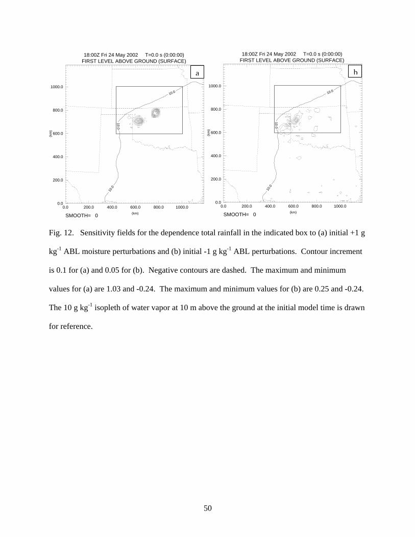
50
10.0
10.0
10.0
0.0 200.0 400.0 600.0 800.0 1000.00.0
200.0
400.0
600.0
800.0
1000.0
(km)
(km
)
FIRST LEVEL ABOVE GROUND (SURFACE) 18:00Z Fri 24 May 2002 T=0.0 s (0:00:00)
SMOOTH= 0
10.0
10.0
10.0
0.0 200.0 400.0 600.0 800.0 1000.00.0
200.0
400.0
600.0
800.0
1000.0
(km) (
km)
FIRST LEVEL ABOVE GROUND (SURFACE) 18:00Z Fri 24 May 2002 T=0.0 s (0:00:00)
MIN=1.928 MAX=16.05 inc=0SMOOTH= 0
Fig. 12. Sensitivity fields for the dependence total rainfall in the indicated box to (a) initial +1 g
kg-1 ABL moisture perturbations and (b) initial -1 g kg-1 ABL perturbations. Contour increment
is 0.1 for (a) and 0.05 for (b). Negative contours are dashed. The maximum and minimum
values for (a) are 1.03 and -0.24. The maximum and minimum values for (b) are 0.25 and -0.24.
The 10 g kg-1 isopleth of water vapor at 10 m above the ground at the initial model time is drawn
for reference.
a b

51
10.0
10.0
10.0
0.0 200.0 400.0 600.0 800.0 1000.00.0
200.0
400.0
600.0
800.0
1000.0
(km)
(km
)
FIRST LEVEL ABOVE GROUND (SURFACE) 18:00Z Fri 24 May 2002 T=0.0 s (0:00:00)
SMOOTH= 1
10.0
10.0
10.0
0.0 200.0 400.0 600.0 800.0 1000.00.0
200.0
400.0
600.0
800.0
1000.0
(km)
(km
)
FIRST LEVEL ABOVE GROUND (SURFACE) 18:00Z Fri 24 May 2002 T=0.0 s (0:00:00)
SMOOTH= 3
Fig. 13. Sensitivity fields for the dependence total rainfall in the indicated box to (a) initial
+1 m3 m-3 soil moisture perturbations and (b) initial +1 m s-1 ABL meridional wind speed
perturbations. Contour increment is 0.05 for (a) and 0.01 for (b). (a) was smoothed once and (b)
was smoothed three times using a nine-point smoother. Negative contours are dashed. The
maximum and minimum values for (a) are 0.10 and -0.13 (0.18 and -0.13 unsmoothed). The
maximum and minimum values for (b) are 0.034 and -0.028 (0.055 and -0.044 unsmoothed).
The 10 g kg-1 isopleth of water vapor at 10 m above the ground at the initial model time is drawn
for reference.
a b

52
10.0
10.0
10.0
0.0 200.0 400.0 600.0 800.0 1000.00.0
200.0
400.0
600.0
800.0
1000.0
(km)
(km
)
FIRST LEVEL ABOVE GROUND (SURFACE) 18:00Z Fri 24 May 2002 T=0.0 s (0:00:00)
20.040.0
SMOOTH= 0
10.0
10.0
10.0
0.0 200.0 400.0 600.0 800.0 1000.00.0
200.0
400.0
600.0
800.0
1000.0
(km) (
km)
FIRST LEVEL ABOVE GROUND (SURFACE) 18:00Z Fri 24 May 2002 T=0.0 s (0:00:00)
MIN=1.928 MAX=16.05 inc=0.
40.0
SMOOTH= 0
Fig. 14. Forecast accumulated precipitation which fell in two model runs with a 1 g kg-1
perturbation in ABL moisture at the location and of the size indicated by the drawn box in (a)
northwestern Oklahoma, and (b) north central Oklahoma. Contour increments are 10 mm. The
local maximum along the Kansas-Oklahoma border in (a) is 120 mm. The local maximum in
southeast Kansas in (b) is 30 mm. The 10 g kg-1 isopleth of water vapor at 10 m above the
ground at the initial model time is drawn for reference.
a b

53
10.0
10.0
10.0
0.0 200.0 400.0 600.0 800.0 1000.00.0
200.0
400.0
600.0
800.0
1000.0
(km)
(km
)
FIRST LEVEL ABOVE GROUND (SURFACE) 18:00Z Fri 24 May 2002 T=0.0 s (0:00:00)
SMOOTH= 1
10.0
10.0
10.0
0.0 200.0 400.0 600.0 800.0 1000.00.0
200.0
400.0
600.0
800.0
1000.0
(km)
(km
)
FIRST LEVEL ABOVE GROUND (SURFACE) 18:00Z Fri 24 May 2002 T=0.0 s (0:00:00)
0.0
SMOOTH= 1
Fig. 15. Sensitivity to average 10 m wind speed in a 36 km square box at two locations to initial
ABL 1 g kg-1 moisture perturbations. Box for response function is drawn in each figure at (a)
northwest Texas and (b) southeast Oklahoma. Contour increment is 0.01 in (a) and 0.0125 in
(b). A nine point smoother was applied to both figures once. Negative contours are dashed. The
10 g kg-1 isopleth of water vapor at 10 m above the ground at the initial model time is drawn for
reference.
a b

54
10.0
10.0
10.0
0.0 200.0 400.0 600.0 800.0 1000.00.0
200.0
400.0
600.0
800.0
1000.0
(km)
(km
)
FIRST LEVEL ABOVE GROUND (SURFACE) 18:00Z Fri 24 May 2002 T=0.0 s (0:00:00)
MIN=1.928 MAX=16.05 inc=0.
-9.6
-9.6
-9.6
-9.6
-9.6
-9.6
-9.2
-9.2
-9.2
-9.2
-9.2
-8.8
-8.8
-8.8
-8.8
-8.8
-8.4
-8.4
-8.4
-8.4
-8.4
-8.0
-8.0
-8.0
-8.0
-8.0
-7.6
-7.6
-7.6
-7.6
-7.6
-7.2
-7.2
-7.2
-7.2
-7.2
-6.8
-6.8
-6.8
-6.8
-6.8
-6.4
-6.4
-6.4
-6.4
-6.4
-6.4
-6.0
-6.0
-6.0
-6.0
-6.0
-6.0
-5.6
-5.6
-5.6
-5.6
-5.6
-5.6
-5.2
-5.2
-5.2
-5.2
-5.2
-5.2
-4.8
-4.8
-4.8
-4.8
-4.8
-4.8
-4.4
-4.4-4.4
-4.4
-4.4
-4.0
-4.0-4.0
-4.0
-4.0
-3.6
-3.6
-3.6
-3.6
-3.6
-3.2
-3.2-3.2
-3.2
-3.2
-2.8
-2.8
-2.8-2
.8
-2.8
-2.4
-2.4
-2.4-2.4
-2.4
-2.0
-2.0
-2.0
-2.0 -2.0
-1.6
-1.6
-1.6
-1.6
-1.6
-1.2
-1.2
-1.2
-1.2
-1.2
-0.8
-0.8
-0.8
-0.8
-0.8
-0.8
-0.4
-0.4
-0.4
-0.4
-0.4
-0.4
0.4
0.4
0.4
0.4
0.4
0.4
0.8
0.8
0.8
1.2
1.2
1.6
1.62
.0
2.4
2.8
3.2
3.6
4.0
4.4
4.8
5.2
5.6
6.0
6.4
6.8
7.2
7.6
8.0
8.4
8.8
9.2
9.6
10.0
SMOOTH= 5
10.0
10.0
10.0
0.0 200.0 400.0 600.0 800.0 1000.00.0
200.0
400.0
600.0
800.0
1000.0
(km)
(km
)
FIRST LEVEL ABOVE GROUND (SURFACE) 18:00Z Fri 24 May 2002 T=0.0 s (0:00:00)
-4.4-4.0
-3.6
-3.2-2.8-2
.8
-2.4-2.0
-2.0
-1.6
-1.6
-1.2
-1.2
-0.8
-0.8
-0.8
-0.8
-0.4
-0.4
-0.4
-0.4
-0.4
-0.4
0.4
0.4
0.4
0.4
0.4
0.4
0.4
0.4
0.4
0.4
0.8
0.8
0.8
0.8
0.8
1.2
1.2 1.2
1.6
SMOOTH= 5 Fig. 16. Difference in forecast pressure field between forecast with a 1 g kg-1 perturbation in
ABL moisture and the forecast with no perturbation. Location and size of perturbation is
indicated by a box. (a) Perturbation in northwestern Oklahoma. (b) Perturbation in north central
Texas. Contour increment was 0.2 Pa and negative contours are dashed. Contours in (a) above
10 Pa and below -10 Pa were not drawn. A nine point smoother was applied to both (a) and (b)
five times. The unsmoothed maxima (minima) for (a) were 367 (-535) Pa and 19 (-38) Pa for
(b).
a b