Embed Size (px)
Citation preview

Chapter 18
SENSITIVITY ANALYSIS OFBAYESIAN NETWORKS USED INFORENSIC INVESTIGATIONS
Michael Kwan, Richard Overill, Kam-Pui Chow, Hayson Tse, FrankLaw and Pierre Lai
Abstract Research on using Bayesian networks to enhance digital forensic inves-tigations has yet to evaluate the quality of the output of a Bayesiannetwork. The evaluation can be performed by assessing the sensitivityof the posterior output of a forensic hypothesis to the input likelihoodvalues of the digital evidence. This paper applies Bayesian sensitivityanalysis techniques to a Bayesian network model for the well-known Ya-hoo! case. The analysis demonstrates that the conclusions drawn fromBayesian network models are statistically reliable and stable for smallchanges in evidence likelihood values.
Keywords: Forensic investigations, Bayesian networks, sensitivity analysis
1. Introduction
Research on applying Bayesian networks to criminal investigations ison the rise [7–9, 12]. The application of Bayes’ theorem and graph theoryprovides a means to characterize the causal relationships among variables[16]. In terms of forensic science, these correspond to the hypothesis andevidence. When constructing a Bayesian network, the causal structureand conditional probability values come from multiple experiments orexpert opinion.
The main difficulties in constructing a Bayesian network are in know-ing what to ask experts and in assessing the accuracy of their responses.When an assessment is made from incomplete estimations or inconsis-tent beliefs, the resulting posterior output is inaccurate or “sensitive”[4]. Therefore, when applying a Bayesian network model, the investi-gator must understand the certainty of the conclusions drawn from the

232 ADVANCES IN DIGITAL FORENSICS VII
model. Sensitivity analysis provides a means to evaluate the possibleinferential outcomes of a Bayesian network to gain this understanding[11].
This paper applies sensitivity analysis techniques to evaluate the cor-rectness of a Bayesian network model for the well-known Yahoo! case [3].The Bayesian network was constructed using details from the convictionreport, which describes the evidence that led to the conviction of the de-fendant [7]. The analysis tests the sensitivity of the hypothesis to smalland large changes in the likelihood of individual pieces of evidence.
2. Sensitivity Analysis
The accuracy of a Bayesian network depends on the robustness of theposterior output to changes in the input likelihood values [5]. A Bayesiannetwork is robust if it exhibits a lack of posterior output sensitivity tosmall changes in the likelihood values. Sensitivity analysis is importantdue to the practical difficulty of precisely assessing the beliefs and pref-erences underlying the assumptions of a Bayesian model. Sensitivityanalysis investigates the properties of a Bayesian network by studyingits output variations arising from changes in the input likelihood values[15].
A common approach to assess the sensitivity is to iteratively vary eachlikelihood value over all possible combinations and evaluate the effectson the posterior output [6]. If large changes in the likelihood valuesproduce a negligible effect on the posterior output, then the evidenceis sufficiently influential and has little to no impact on the model. Onthe other hand, if small changes cause the posterior output to changesignificantly, then it is necessary to review the network structure andthe prior probability values.
Since the probability distributions of the evidence likelihood valuesand hypothesis posteriors in a Bayesian network constructed for a digitalforensic investigation are mostly discrete, parameter sensitivity analy-sis can be used to evaluate the sensitivity of the Bayesian network forthe Yahoo! case. Three approaches, bounding sensitivity function, sen-sitivity value and vertex proximity, are used to determine the boundingsensitivity of each piece of evidence and its robustness under small andlarge variations in its likelihood value.
2.1 Bounding Sensitivity Function
Parameter sensitivity analysis evaluates the posterior output basedon variations in the evidence provided. It is impractical – possibly,computationally intractable – to perform a full sensitivity analysis that
Kwan, et al. 233
varies the likelihood values one at a time while keeping the other valuesfixed [10]. One solution to the intractability problem is to use a boundingsensitivity function to select functions that have a high sensitivity [13].
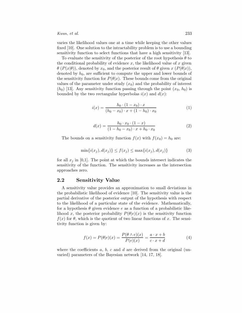
To evaluate the sensitivity of the posterior of the root hypothesis θ tothe conditional probability of evidence x, the likelihood value of x givenθ (P (x|θ)), denoted by x0, and the posterior result of θ given x (P (θ|x)),denoted by h0, are sufficient to compute the upper and lower bounds ofthe sensitivity function for P (θ|x). These bounds come from the originalvalues of the parameter under study (x0) and the probability of interest(h0) [13]. Any sensitivity function passing through the point (x0, h0) isbounded by the two rectangular hyperbolas i(x) and d(x):
i(x) =h0 · (1 − x0) · x
(h0 − x0) · x + (1 − h0) · x0(1)
d(x) =h0 · x0 · (1 − x)
(1 − h0 − x0) · x + h0 · x0(2)
The bounds on a sensitivity function f(x) with f(x0) = h0 are:
min{i(xj), d(xj)} ≤ f(xj) ≤ max{i(xj), d(xj)} (3)
for all xj in [0,1]. The point at which the bounds intersect indicates thesensitivity of the function. The sensitivity increases as the intersectionapproaches zero.
2.2 Sensitivity Value
A sensitivity value provides an approximation to small deviations inthe probabilistic likelihood of evidence [10]. The sensitivity value is thepartial derivative of the posterior output of the hypothesis with respectto the likelihood of a particular state of the evidence. Mathematically,for a hypothesis θ given evidence e as a function of a probabilistic like-lihood x, the posterior probability P (θ|e)(x) is the sensitivity functionf(x) for θ, which is the quotient of two linear functions of x. The sensi-tivity function is given by:
f(x) = P (θ|e)(x) =P (θ ∧ e)(x)
P (e)(x)=
a · x + b
c · x + d(4)
where the coefficients a, b, c and d are derived from the original (un-varied) parameters of the Bayesian network [14, 17, 18].

234 ADVANCES IN DIGITAL FORENSICS VII
The sensitivity of a likelihood value is the absolute value of the firstderivative of the sensitivity function at the original likelihood value [14]:
!!!!a · d − b · c(c · x + d)2
!!!! (5)
This sensitivity value describes the change in the posterior output of thehypothesis for small variations in the likelihood of the evidence understudy. The larger the sensitivity value, the less robust the posterioroutput of the hypothesis [14]. In other words, a likelihood value witha large sensitivity value is prone to generate an inaccurate posterioroutput. If the sensitivity value is less than one, then a small change inthe likelihood value has a minimal effect on the result of the posterioroutput of the hypothesis [17].
2.3 Vertex Proximity
Even if a Bayesian network is robust to small changes in its evidencelikelihood values, it is also necessary to assess if the network is robustto large variations in the likelihood values [17]. The impact of a largervariation in a likelihood value, the vertex proximity, depends on thelocation of the vertex of the sensitivity function. Calculating the vertexproximity assumes that the sensitivity function has a hyperbolic formexpressed as:
f(x) =r
x − s+ t where s = −d
c; t =
a
c; r =
b
c+ s · t (6)
Given a sensitivity function defined by 0 ≤ f(x) ≤ 1, the two-dimensional space (x, f(x)) is bounded by the unit window [0,1] [14].The vertex is a point where the sensitivity value (| a·d−b·c
(c·x+d)2 |) is equal to
one. Because the rectangular hyperbola extends indefinitely, the verti-cal asymptotes of the hyperbola may lie outside the unit window, eithers < 0 or s > 1.
The vertex proximity expression:
xv = {s +"
|r| if s < 0 or s −"|r| if s > 1} (7)
is based on the vertex value with respect to the likelihood value of s[17]. If the original likelihood value is close to the value of xv, thenthe posterior output may possess a high degree of sensitivity to largevariations in the likelihood value [17].

Kwan, et al. 235
3. Bayesian Network for the Yahoo! Case
This section describes the application of the bounding sensitivity, sen-sitivity value and vertex proximity techniques to evaluate the robustnessof a Bayesian network constructed for the Yahoo! case [7]. Constructinga Bayesian network for a forensic investigation begins with the estab-lishment of the top-most hypothesis. Usually, this hypothesis representsthe main issue to be resolved. In the Yahoo! case, the hypothesis H isthat the seized computer was used to send the subject file as an emailattachment using a specific Yahoo! email account.
The hypothesis H is the root node of the Bayesian network and is theancestor of every other node in the network. The unconditional (prior)probabilities are: P (H =Yes) = 0.5 and P (H =No) = 0.5.
There are six sub-hypotheses that are dependent on the main hypoth-esis H. The six sub-hypothesis are events that should have occurred ifthe file in question had been sent by the suspect’s computer via Yahoo!web-mail. The sub-hypotheses (states: Yes and No) are:
H1: Linkage between the subject file and the suspect’s computer.
H2: Linkage between the suspect and the computer.
H3: Linkage between the suspect and the ISP.
H4: Linkage between the suspect and the Yahoo! email account.
H5: Linkage between the computer and the ISP.
H6: Linkage between the computer and the Yahoo! email account.
Table 1 lists the digital evidence DEi (states: Yes, No and Uncertain)associated with the six sub-hypotheses.
Since there are no observations of the occurrences of the six sub-hypotheses, their conditional probability values cannot be predicted us-ing frequentist approaches. Therefore, an expert was asked to subjec-tively assign the probabilities used in this study (Table 2).
Table 3 presents the conditional probability values of the fourteenpieces of digital evidence given the associated sub-hypotheses.
3.1 Posterior Probabilities
Figures 1 and 2 show the posterior probabilities of H when H1 . . . H6
are Yes and No, respectively. The upper and lower bounds of H – theseized computer was used to send the subject file as an email attach-ment via the Yahoo! email account – are 0.972 and 0.041, respectively.However, these posterior results are not justified until the sensitivity ofthe Bayesian network is evaluated.

236 ADVANCES IN DIGITAL FORENSICS VII
Table 1. Sub-hypotheses and the associated evidence.
Sub-Hypot. Evidence Description
H1 DE1 Subject file exists on the computerH1 DE2 Last access time of the subject file is after the IP
address assignment time by the ISPH1 DE3 Last access time of the subject file is after or is close
to the sent time of the Yahoo! emailH2 DE4 Files on the computer reveal the identity of the sus-
pectH3 DE5 ISP subscription details (including the assigned IP
address) match the suspect’s particularsH4 DE6 Subscription details of the Yahoo! email account (in-
cluding the IP address that sent the email) matchthe suspect’s particulars
H5 DE7 Configuration settings of the ISP Internet accountare found on the computer
H5 DE8 Log data confirms that the computer was poweredup at the time the email was sent
H5 DE9 Web browser (e.g., Internet Explorer) or email pro-gram (e.g., Outlook) was found to be activated atthe time the email was sent
H5 DE10 Log data reveals the assigned IP address and theassignment time by the ISP to the computer
H5 DE11 Assignment of the IP address to the suspect’s ac-count is confirmed by the ISP
H6 DE12 Internet history logs reveal that the Yahoo! emailaccount was accessed by the computer
H6 DE13 Internet cache files reveal that the subject file wassent as an attachment from the Yahoo! email ac-count
H6 DE14 IP address of the Yahoo! email with the attachedfile is confirmed by Yahoo!
Table 2. Likelihood of H1 . . . H6 given H .
H1, H5, H6 H2, H3, H4
H Y N Y N
Y 0.65 0.35 0.8 0.2N 0.35 0.65 0.2 0.8
4. Sensitivity Analysis Results
This section presents the results of the sensitivity analysis conductedon the Bayesian network for the Yahoo! case.

Kwan, et al. 237
Table 3. Probabilities of DE1 . . . DE14 given Hi.
Y N U Y N U Y N UHi DE1, i = 1 DE2, DE3, i = 1 DE4, i = 2
Y 0.85 0.15 0.00 0.80 0.15 0.05 0.75 0.20 0.05N 0.15 0.85 0.00 0.15 0.80 0.05 0.20 0.75 0.05
DE5, i = 3 DE6, i = 4 DE7, DE8, DE10, i = 5
Y 0.70 0.25 0.05 0.10 0.85 0.05 0.70 0.25 0.05N 0.25 0.70 0.05 0.05 0.90 0.05 0.25 0.70 0.05
DE9, DE11, i = 5 DE12, DE13, i = 6 DE14, i = 6
Y 0.80 0.15 0.05 0.70 0.25 0.05 0.80 0.15 0.05N 0.15 0.80 0.05 0.25 0.70 0.05 0.15 0.80 0.05
Yes 0.972
No 0.028
H
Yes 0.996
No 0.004
H1
Yes 0.925
No 0.075
H2
Yes 0.904
No 0.096
H3
Yes 0.999
No 0.001
H5
Yes 0.986
No 0.014
H6
Yes 0.873
No 0.127
H4
Yes 1.000
No 0.000
Un 0.000
DE1
Yes 1.000
No 0.000
Un 0.000
DE2
Yes 1.000
No 0.000
Un 0.000
DE3
Yes 1.000
No 0.000
Un 0.000
DE4
Yes 1.000
No 0.000
Un 0.000
DE5
Yes 1.000
No 0.000
Un 0.000
DE8
Yes 1.000
No 0.000
Un 0.000
DE9
Yes 1.000
No 0.000
Un 0.000
DE10
Yes 1.000
No 0.000
Un 0.000
DE11
Yes 1.000
No 0.000
Un 0.000
DE14
Yes 1.000
No 0.000
Un 0.000
DE13
Yes 1.000
No 0.000
Un 0.000
DE12
Yes 1.000
No 0.000
Un 0.000
DE6
Yes 1.000
No 0.000
Un 0.000
DE7
Figure 1. Posterior probabilities when DE1 . . . DE14 are Yes.
4.1 Bounding Sensitivity Analysis
The sensitivity of the posterior outputs of the root hypothesis H tothe conditional probabilities of evidence DE1 . . . DE14 is computedusing Equation (4). To illustrate the process, we compute the boundingsensitivity function for H against the likelihood of DE1.
From Table 3, the likelihood of DE1 (subject file exists on the sus-pect’s computer) given H1 (linkage between the subject file and thecomputer), i.e., P (DE1|H1) is equal to 0.85 (x0). As shown in Figure 3,if DE1 is observed, the posterior output of the root hypothesis H, i.e.,DE1 (P (H|DE1)), is equal to 0.60 (h0).

238 ADVANCES IN DIGITAL FORENSICS VII
Yes 0.041
No 0.959
H
Yes 0.004
No 0.996
H1
Yes 0.081
No 0.919
H2
Yes 0.103
No 0.897
H3
Yes 0.001
No 0.999
H5
Yes 0.014
No 0.986
H6
Yes 0.215
No 0.785
H4
Yes 0.000
No 1.000
Un 0.000
DE1
Yes 0.000
No 1.000
Un 0.000
DE2
Yes 0.000
No 1.000
Un 0.000
DE3
Yes 0.000
No 1.000
Un 0.000
DE4
Yes 0.000
No 1.000
Un 0.000
DE5
Yes 0.000
No 1.000
Un 0.000
DE8
Yes 0.000
No 1.000
Un 0.000
DE9
Yes 0.000
No 1.000
Un 0.000
DE10
Yes 0.000
No 1.000
Un 0.000
DE11
Yes 0.000
No 1.000
Un 0.000
DE14
Yes 0.000
No 1.000
Un 0.000
DE13
Yes 0.000
No 1.000
Un 0.000
DE12
Yes 0.000
No 1.000
Un 0.000
DE6
Yes 0.000
No 1.000
Un 0.000
DE7
Figure 2. Posterior probabilities when DE1 . . . DE14 are No.
Yes 0.605
No 0.395
H
Yes 0.850
No 0.150
H1
Yes 1.000
No 0.000
Un 0.000
DE1
Yes 0.702
No 0.248
Un 0.050
DE2
Yes 0.702
No 0.248
Un 0.050
DE3
Figure 3. Posterior probability of H when DE1 is Yes.
Upon applying Equations (1) and (2), the sensitivity functions i(x)and d(x) are given by:
i(x) =h0 · (1 − x0) · x
(h0 − x0) · x + (1 − h0) · x0=
0.09075x
0.33575 − 0.245x(8)
d(x) =h0 · x0 · (1 − x)
(1 − h0 − x0) · x + h0 · x0=
0.51425 − 0.51425x
0.51425 − 0.455x(9)
Figure 4(a) presents the bounding sensitivity functions for the pos-teriors of hypothesis H to P (DE1|H1). In particular, it shows the plotof the i(x) and d(x) functions, which is the bounding sensitivity ofP (H|DE1) against P (DE1|H1). Note that a significant shift in the es-timated bounds for P (H|DE1) occurs when P (DE1|H1) is greater than0.85. Because the shift is large, the hypothesis is not sensitive to changesin DE1.
The bounds of P (H|DE2) . . . P (H|DE14) and the bounds of P (DE2
|H2) . . . P (DE14|H6) do not produce significant changes in the boundsfor the posterior output and are not sensitive to changes in the likeli-

Kwan, et al. 239
0
0.1
0.2
0.3
0.4
0.5
0.6
0.7
0.8
0.9
1
0 0.2 0.4 0.6 0.8 1
P(H
| D
E1)
P(DE1 | H1)
i(x)
d(x)
0
0.1
0.2
0.3
0.4
0.5
0.6
0.7
0.8
0.9
1
0 0.2 0.4 0.6 0.8 1
P(H
| DE6)
P(DE6 | H4)
i(x)
d(x)
(a) (b)
Figure 4. Bounding sensitivity functions.
hood values. The most sensitive bound is for the sensitivity function ofP (H|DE6), which is less than 0.1 according to Figure 4(b). Note thatFigure 4(b) shows the bounding sensitivity for the posterior probabili-ties of the root hypothesis H to P (DE6|H4). Although the likelihoodof DE6 is more sensitive than the likelihoods of the other pieces of digi-tal evidence, the robustness of the posterior results with respect to theelicited conditional probabilities in the Yahoo! Bayesian network is stillnot clear. Therefore, the sensitivity values and vertex proximities forthe evidence must also be assessed to ascertain the robustness of theBayesian network.
4.2 Sensitivity Value Analysis
To illustrate the sensitivity value analysis technique, we evaluate thesensitivity of sub-hypothesis H1 (linkage between the subject file and thesuspect’s computer) to the likelihood value of evidence DE1 (subjectfile exists on the computer). The sensitivity value analysis evaluatesthe probability of interest, P (H1|DE1), for a variation in the likelihoodvalue of P (DE1|H1). This requires a sensitivity function that expressesP (H1|DE1) in terms of x = P (DE1|H1):
P (H1|DE1)(x) =P (DE1|H1)P (H1)
P (DE1)(10)
Rewriting the numerator P (DE1|H1)P (H1) as P (H1)x + 0 yields thecoefficient values a = P (H1) and b = 0. Rewriting the denomina-tor as P (DE1) = P (DE1|H1)P (H1) + P (DE1|H1)P (H1) = P (H1)x +P (DE1|H1)P (H1) yields the coefficient values c = P (H1) and d =P (DE1|H1)P (H1).
Since P (H1) = 0.5 and P (DE1|H1) = 0.15 (from Table 3), the co-efficients of the sensitivity function are: a = 0.5, b = 0, c = 0.5

240 ADVANCES IN DIGITAL FORENSICS VII
Table 4. Sensitivity values and effects on posterior outputs.
Evidence Elicited Sensitivity Function Sensitivity Effect onValue Coefficients Value Posterior
a b c d
DE1 0.85 0.5 0 0.5 0.075 0.150 Hardly changesDE2 0.80 0.5 0 0.5 0.075 0.166 Hardly changesDE3 0.80 0.5 0 0.5 0.075 0.166 Hardly changesDE4 0.75 0.5 0 0.5 0.100 0.222 Hardly changesDE5 0.70 0.5 0 0.5 0.125 0.250 Hardly changesDE6 0.10 0.5 0 0.5 0.025 0.045 Hardly changesDE7 0.70 0.5 0 0.5 0.125 0.250 Hardly changesDE8 0.70 0.5 0 0.5 0.125 0.250 Hardly changesDE9 0.80 0.5 0 0.5 0.075 0.166 Hardly changesDE10 0.70 0.5 0 0.5 0.125 0.250 Hardly changesDE11 0.80 0.5 0 0.5 0.075 0.166 Hardly changesDE12 0.70 0.5 0 0.5 0.125 0.250 Hardly changesDE13 0.70 0.5 0 0.5 0.125 0.250 Hardly changesDE14 0.80 0.5 0 0.5 0.075 0.166 Hardly changes
and d = 0.075. Upon applying Equation (5), the sensitivity value ofP (H1|DE1) against P (DE1|H1) is:
!!!!a · d − b · c(c · x + d)2
!!!! =
!!!!0.5 · 0.075 − 0 · 0.5(0.5 · 0.85 + 0.075)2
!!!! = 0.15 (11)
As noted in [17], if the sensitivity value is less than one, then a smallchange in the likelihood value has a minimal effect on the posterior out-put of a hypothesis. Table 4 shows sensitivity values that express theeffects of small changes in evidence likelihood values on the posterior out-puts of the related sub-hypotheses. Note that all the sensitivity valuesare less than one. Therefore, it can be concluded that the Bayesian net-work is robust to small variations in the elicited conditional probabilities.Since priors of the evidence are computed from the elicited probabilities,it can also be concluded that the Yahoo! Bayesian network is robust tosmall variations in the evidence likelihood values.
4.3 Vertex Proximity Analysis
Although the Yahoo! Bayesian network is robust to small changes inevidence likelihood values, it is also necessary to assess its robustnessto large variations in the conditional probabilities. Table 5 shows theresults of the vertex likelihood (xv) computation using Equation (7) forDE1 . . . DE14.

Kwan, et al. 241
Table 5. Sensitivity values and effects on posterior outputs.
Evidence Elicited s t r xv |xv − x0|Value (x0)
DE1 0.85 -0.15 1 -0.15 0.237 0.613DE2 0.80 -0.15 1 -0.15 0.237 0.563DE3 0.80 -0.15 1 -0.15 0.237 0.563DE4 0.75 -0.20 1 -0.20 0.247 0.503DE5 0.70 -0.25 1 -0.25 0.250 0.450DE6 0.10 -0.05 1 -0.05 0.174 0.074DE7 0.70 -0.25 1 -0.25 0.250 0.450DE8 0.70 -0.25 1 -0.25 0.250 0.450DE9 0.80 -0.15 1 -0.15 0.237 0.563DE10 0.70 -0.25 1 -0.25 0.250 0.450DE11 0.80 -0.15 1 -0.15 0.237 0.613DE12 0.70 -0.25 1 -0.25 0.250 0.450DE13 0.70 -0.25 1 -0.25 0.250 0.450DE14 0.80 -0.15 1 -0.15 0.237 0.563
Table 5 shows sensitivity values expressing the effects of large changesin evidence likelihood values on the posterior outputs of related sub-hypotheses. Based on the small sensitivity values in Table 4 and thelack of vertex proximity shown in Table 5, the posterior outputs of thesub-hypotheses H1, H2, H3, H5 and H6 are not sensitive to variationsin the likelihood values of DE1 . . . DE5 and DE7 . . . DE14.
However, for digital evidence DE6 and sub-hypothesis H4, the elicitedprobability of 0.1 is close to the vertex value of 0.174; thus, the elicitedprobability of DE6 exhibits a degree of vertex proximity. In other words,the posterior result of H4 (linkage between the suspect and the Yahoo!email account) is sensitive to the variation in the likelihood value of DE6
even though the sensitivity value for DE6 is small.Although the Yahoo! Bayesian network is robust, the elicitation of the
likelihood value of DE6 (subscription details of the Yahoo! email accountmatch the suspect’s particulars) given sub-hypothesis H4 (P (DE6|H4))is the weakest node in the network. The weakest node is most susceptibleto change and is, therefore, the best place to attack the case. This meansthat digital evidence DE6 is of the greatest value to defense attorneysand prosecutors.
5. Conclusions
The bounding sensitivity function, sensitivity value and vertex prox-imity are useful techniques for analyzing the sensitivity of Bayesian net-works used in forensic investigations. The analysis verifies that the

242 ADVANCES IN DIGITAL FORENSICS VII
Bayesian network developed for the celebrated Yahoo! case is reliableand accurate. The analysis also reveals that evidence related to the hy-pothesis that the subscription details of the Yahoo! email account matchthe suspect’s particulars is the most sensitive node in the Bayesian net-work. To ensure accuracy, the investigator must critically review theelicitation of this evidence because a change to this node has the great-est effect on the network output.
The one-way sensitivity analysis presented in this paper varies onelikelihood value at a time. It is possible to perform n-way analysis of aBayesian network, but the mathematical functions become very compli-cated [17]. Given that digital evidence is becoming increasingly impor-tant in court proceedings, it is worthwhile to conduct further research onmulti-parameter, higher-order sensitivity analysis [2] to ensure that ac-curate analytical conclusions can be drawn from the probabilistic resultsobtained with Bayesian networks.
References
[1] J. Berger, An Overview of Robust Bayesian Analysis, TechnicalReport 93-53C, Department of Statistics, Purdue University, WestLafayette, Indiana, 1993.
[2] H. Chan and A. Darwiche, Sensitivity analysis in Bayesian net-works: From single to multiple parameters, Proceedings of the Twen-tieth Conference on Uncertainty in Artificial Intelligence, pp. 67–75,2004.
[3] Changsha Intermediate People’s Court of Hunan Province, Rea-sons for Verdict, First Trial Case No. 29, Changsha IntermediateCriminal Division One Court, Changsha, China (www.pcpd.org.hk/english/publications/files/Yahoo annex.pdf), 2005.
[4] M. Druzdzel and L. van der Gaag, Elicitation of probabilities for be-lief networks: Combining qualitative and quantitative information,Proceedings of the Eleventh Conference on Uncertainty in ArtificialIntelligence, pp. 141–148, 1995.
[5] J. Ghosh, M. Delampady and T. Samanta, An Introduction toBayesian Analysis: Theory and Methods, Springer, New York, 2006.
[6] J. Gill, Bayesian Methods: A Social and Behavioral Sciences Ap-proach, Chapman and Hall, Boca Raton, Florida, 2002.
[7] M. Kwan, K. Chow, P. Lai, F. Law and H. Tse, Analysis of thedigital evidence presented in the Yahoo! case, in Advances in DigitalForensics V, G. Peterson and S. Shenoi (Eds.), Springer, Heidelberg,Germany, pp. 241–252, 2009.
Kwan, et al. 243
[8] M. Kwan, K. Chow, F. Law and P. Lai, Reasoning about evidenceusing Bayesian networks, in Advances in Digital Forensics IV, I. Rayand S. Shenoi (Eds.), Springer, Boston, Massachusetts, pp. 275–289,2008.
[9] M. Kwan, R. Overill, K. Chow, J. Silomon, H. Tse, F. Law and P.Lai, Evaluation of evidence in Internet auction fraud investigations,in Advances in Digital Forensics VI, K. Chow and S. Shenoi (Eds.),Springer, Heidelberg, Germany, pp. 121–132, 2010.
[10] K. Laskey, Sensitivity analysis for probability assessments inBayesian networks, IEEE Transactions on Systems, Man and Cy-bernetics, vol. 25(6), pp. 901–909, 1995.
[11] M. Morgan and M. Henrion, Uncertainty: A Guide to Dealing withUncertainty in Quantitative Risk and Policy Analysis, CambridgeUniversity Press, Cambridge, United Kingdom, 1992.
[12] R. Overill, M. Kwan, K. Chow, P. Lai and F. Law, A cost-effectivemodel for digital forensic investigations, in Advances in DigitalForensics V, G. Peterson and S. Shenoi (Eds.), Springer, Heidel-berg, Germany, pp. 231–240, 2009.
[13] S. Renooij and L. van der Gaag, Evidence-invariant sensitivitybounds, Proceedings of the Twentieth Conference on Uncertaintyin Artificial Intelligence, pp. 479–486, 2004.
[14] S. Renooij and L. van der Gaag, Evidence and scenario sensitivitiesin naive Bayesian classifiers, International Journal of ApproximateReasoning, vol. 49(2), pp. 398–416, 2008.
[15] A. Saltelli, M. Ratto, T. Andres, F. Campolongo, J. Cariboni, D.Gatelli, M. Saisana and S. Tarantola, Global Sensitivity Analysis:The Primer, John Wiley, Chichester, United Kingdom, 2008.
[16] F. Taroni, C. Aitken, P. Garbolino and A. Biedermann, BayesianNetwork and Probabilistic Inference in Forensic Science, John Wi-ley, Chichester, United Kingdom, 2006.
[17] L. van der Gaag, S. Renooij and V. Coupe, Sensitivity analysis ofprobabilistic networks, in Advances in Probabilistic Graphical Mod-els, P. Lucas, J. Gamez and A. Salmeron (Eds.), Springer, Berlin,Germany, pp. 103–124, 2007.
[18] H. Wang, I. Rish and S. Ma, Using sensitivity analysis for selec-tive parameter update in Bayesian network learning, Proceedings ofthe AAAI Spring Symposium on Information Refinement and Re-vision for Decision Making: Modeling for Diagnostics, Prognosticsand Prediction, pp. 29–36, 2002.


![Sensitivity or Bayesian model updating: a comparison of ... · nominally identical test pieces by Mares et al. [15,16] using a multivariate gradient-regression approach. Hua et al](https://img.pdfslide.us/doc/110x75/5f03d7077e708231d40b05de/sensitivity-or-bayesian-model-updating-a-comparison-of-nominally-identical.jpg)