Double degree master’s thesis · 30 hec · Advanced level Degree thesis No 764 · ISSN 1401-4084 Uppsala 2012

iiii

Sensitivity Analysis Indicators of Economic Effectiveness - Of investments co-financed by the IPARD Program 2007-2013 in Republic of Macedonia

Vladimir Hristov

Sensitivity analysis indicators of economic effectiveness - Of investments co-financed by the IPARD Program 2007-2013 in Republic of Macedonia Vladimir Hristov Supervisor: Maitreyi Mandal, Swedish University of Agricultural Sciences, Department of Economics Assistant supervisor: Dragan Gjosevski, Ss. Cyril and Methodius, Institute of Agricultural Economics Examiner: Karin Hakelius, Swedish University of Agricultural Sciences, Department of Economics Credits: 30 hec Level: A2E Course title: Degree project in business administration Course code: EX0536 Faculty: Faculty of Natural Resources and Agricultural Sciences Place of publication: Uppsala Year of publication: 2012 Cover picture: John Woudstra, The Age Name of Series: Degree project/SLU, Department of Economics No: 764 ISSN 1401-4084 Online publication: http://stud.epsilon.slu.se Key words: business plan, net present value, internal rate of return, payback method, sensitivity analysis, financial statements, financial analysis, finacial ratios

iii

About this publication

This master thesis was produced within the International Master Program in Agribusiness (120 ECTS) supported by the Swedish International Development Cooperation Agency (Sida) through the project UniCoop. The master program leads to a double degree from two academic institutions: the Faculty of Agricultural Sciences and Food (FASF) at the University “Ss. Cyril and Methodius” (UKIM) in Skopje, Republic of Macedonia (RM) and the Swedish University of Agricultural Sciences (SLU) in Uppsala, Sweden. The master thesis is published at both universities, UKIM and SLU.

Магистерскиот труд е подготвен во рамките на Меѓународните студии по Агробизнис (120 ЕКТС) поддржани од СИДА. Студиите водат кон двојна диплома од страна на две академски институции: Факултетот за земјоделски науки и храна - Скопје (ФЗНХ) при Универзитет „Св. Кирил и Методиј“ во Скопје (УКИМ) и Шведскиот универзитет за земјоделски науки (СЛУ) во Упсала. Магистерскиот труд е објавен на двата универзитета, УКИМ и СЛУ.

iv

Acknowledgements I would like to express my grathitude to the Department of economics at the Swedish University of Agricultural Sciences (SLU) and the Department of Agricultural Economics and Organization at St Cyril and Methodius University in Skopje for giving me an opputunity to upgrade my knowledge on a higher level in the field of Agricultural Economics and management. Second, I would like to thank to the Agency for Financial Support in Agriculture and Rural Development in Republic of Macedonia (AFSARD) for their cooperation and for providing me with all the necesery information. Last but not least, I am especially thankful to my family, but mostly to my father Todor, my mother Olivera, my twin brother Jordan and my sister Milka. At the end, I would like express my special gratitude to my wife Elena who give me support through all these years and bring joy fulness to my everyday life.

v

Abstract/ Summary To the economist an investment is a set of activities in investment capital for the production of economic benefits. As it usually comes to investing large amounts of cash with uncertain results, investment decisions are always risky business decisions. The efficiency of investment projects is evaluated by using economic, financial, technological, ecological-environmental and other efficiency indicators. Finance is the application of economic principles and concepts to business decision making and problem solving. The field of finance can be considered to comprise three broad categories: financial management, investments and financial institutions. The financial analysis in it is broadest sense is analysis that has to do with budgets and finances over time. Within the analysis of the operation is perceived risk and return in order to make better decisions about investing or lending. Such analysis indicated the ability to see into the future, and it is therefore necessary to explain the past and provide a basis for projecting future earnings. The prime aim of this study is to create a model which will create new income opportunities for farmers and promote sustainable agricultural practices. But most important is to get the most realistic indicators of economic effectiveness of investments in the agricultural sector. By understanding these indicators, farmers shall be able to independently evaluate the economic effects of the investments on their business which shall contribute to improvement of their farm management and decision making skills. From the results which are generated by applying the methodology of sensitivity analysis, the conclusion is that in general these findings can help the farmers in terms of improving their planning, facilitate their decision making process and guide their financial health. Also this model allows to identify the investment opportunities, and provide the necessary information’s to facilitate a more efficient allocation and management of risk.

vi

Abbreviations AFSARD – Agency for financial support and rural development CAP - Common Agricultural Policy EU – Europian Union EUR – Euro FADN - Farm Accountancy Data Network FAO - Food and Agricultural Organization of the United Nations GDP – Gross Domestic Product IRR – Internal Rate of Return IPARD - Operational Programme under the EU instrument for Pre-Accession for Rural Development MAFWE - Ministry of Agriculture, Forestry and Water Economy MKD - Macedonian Denar NARDS - National Agricultural and Rural Development Programme NPV – Net Present Value RM – Republic of Macedonia SEAF - Small Enterprise Assistance Funds SSO – State Statistical Office USD – US Dollar

vii

Table of Contents

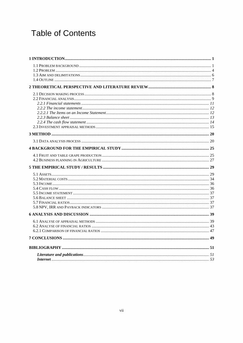
1 INTRODUCTION .............................................................................................................................................. 1 1.1 PROBLEM BACKGROUND ................................................................................................................................ 1 1.2 PROBLEM ....................................................................................................................................................... 4 1.3 AIM AND DELIMITATIONS ............................................................................................................................... 6 1.4 OUTLINE ........................................................................................................................................................ 7

2 THEORETICAL PERSPECTIVE AND LITERATURE REVIEW ............................................................. 8 2.1 DECISION MAKING PROCESS ........................................................................................................................... 8 2.2 FINANCIAL ANALYSIS ..................................................................................................................................... 9

2.2.1 Financial statements ............................................................................................................................ 11 2.2.2 The income statement ........................................................................................................................... 12 2.2.2.1 The Items on an Income Statement .................................................................................................... 12 2.2.3 Balance sheet ....................................................................................................................................... 13 2.2.4 The cash flow statement ....................................................................................................................... 14

2.3 INVESTMENT APPRAISAL METHODS .............................................................................................................. 15 3 METHOD ......................................................................................................................................................... 20

3.1 DATA ANALYSIS PROCESS ............................................................................................................................ 20 4 BACKGROUND FOR THE EMPIRICAL STUDY ..................................................................................... 25

4.1 FRUIT AND TABLE GRAPE PRODUCTION ........................................................................................................ 25 4.2 BUSINESS PLANNING IN AGRICULTURE ........................................................................................................ 27

5 THE EMPIRICAL STUDY / RESULTS ....................................................................................................... 29 5.1 ASSETS ......................................................................................................................................................... 29 5.2 MATERIAL COSTS ......................................................................................................................................... 34 5.3 INCOME ........................................................................................................................................................ 36 5.4 CASH FLOW .................................................................................................................................................. 36 5.5 INCOME STATEMENT .................................................................................................................................... 37 5.6 BALANCE SHEET .......................................................................................................................................... 37 5.7 FINANCIAL RATIOS ....................................................................................................................................... 37 5.8 NPV, IRR AND PAYBACK INDICATORS ........................................................................................................ 37

6 ANALYSIS AND DISCUSSION .................................................................................................................... 39 6.1 ANALYSE OF APPRAISAL METHODS .............................................................................................................. 39 6.2 ANALYSE OF FINANCIAL RATIOS .................................................................................................................. 43 6.2.1 COMPARISON OF FINANCIAL RATIOS ......................................................................................................... 47

7 CONCLUSIONS .............................................................................................................................................. 49

BIBLIOGRAPHY ............................................................................................................................................... 51 Literature and publications .......................................................................................................................... 51 Internet ......................................................................................................................................................... 53

viii

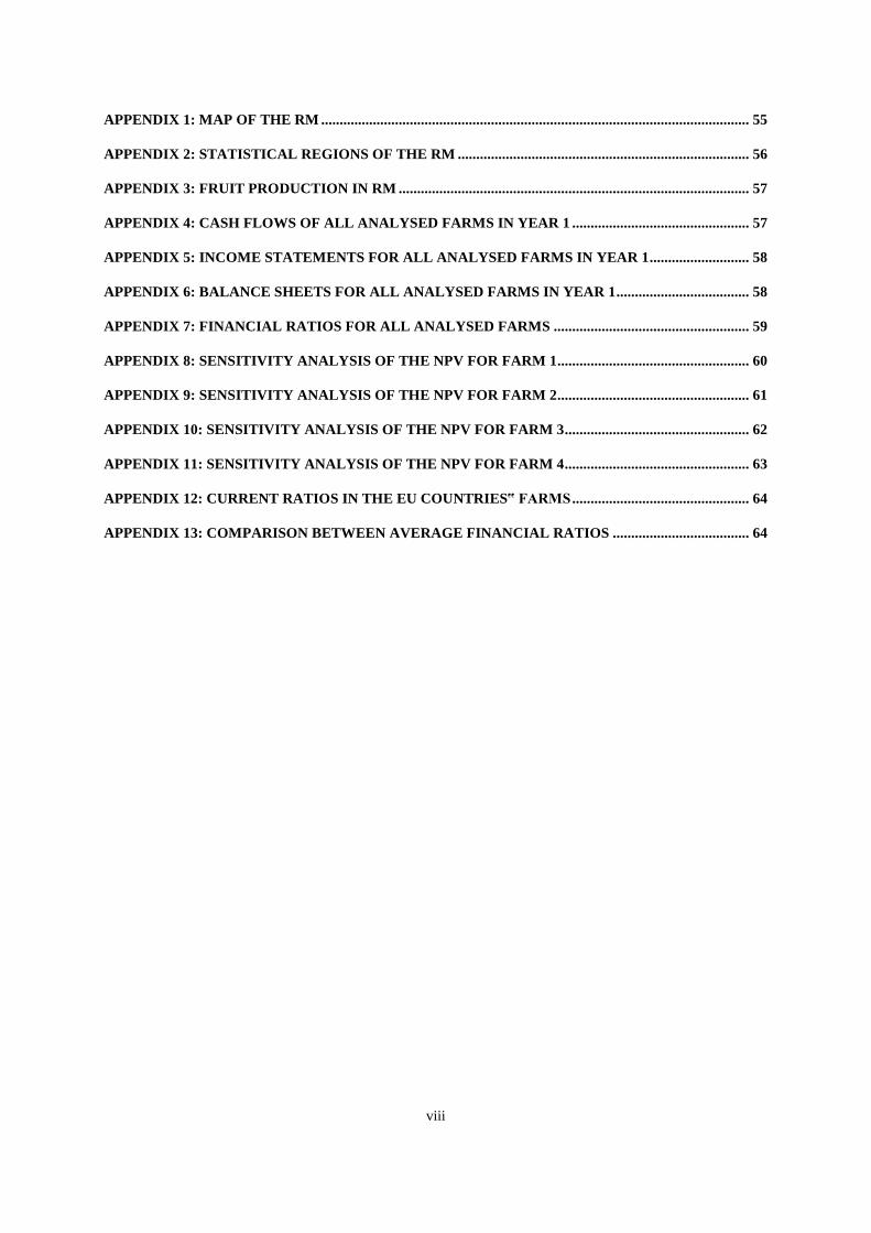
APPENDIX 1: MAP OF THE RM .................................................................................................................... 55

APPENDIX 2: STATISTICAL REGIONS OF THE RM ............................................................................... 56

APPENDIX 3: FRUIT PRODUCTION IN RM ............................................................................................... 57

APPENDIX 4: CASH FLOWS OF ALL ANALYSED FARMS IN YEAR 1 ................................................ 57

APPENDIX 5: INCOME STATEMENTS FOR ALL ANALYSED FARMS IN YEAR 1 ........................... 58

APPENDIX 6: BALANCE SHEETS FOR ALL ANALYSED FARMS IN YEAR 1 .................................... 58

APPENDIX 7: FINANCIAL RATIOS FOR ALL ANALYSED FARMS ..................................................... 59

APPENDIX 8: SENSITIVITY ANALYSIS OF THE NPV FOR FARM 1 .................................................... 60

APPENDIX 9: SENSITIVITY ANALYSIS OF THE NPV FOR FARM 2 .................................................... 61

APPENDIX 10: SENSITIVITY ANALYSIS OF THE NPV FOR FARM 3 .................................................. 62

APPENDIX 11: SENSITIVITY ANALYSIS OF THE NPV FOR FARM 4 .................................................. 63

APPENDIX 12: CURRENT RATIOS IN THE EU COUNTRIES‟ FARMS ................................................ 64

APPENDIX 13: COMPARISON BETWEEN AVERAGE FINANCIAL RATIOS ..................................... 64

ix

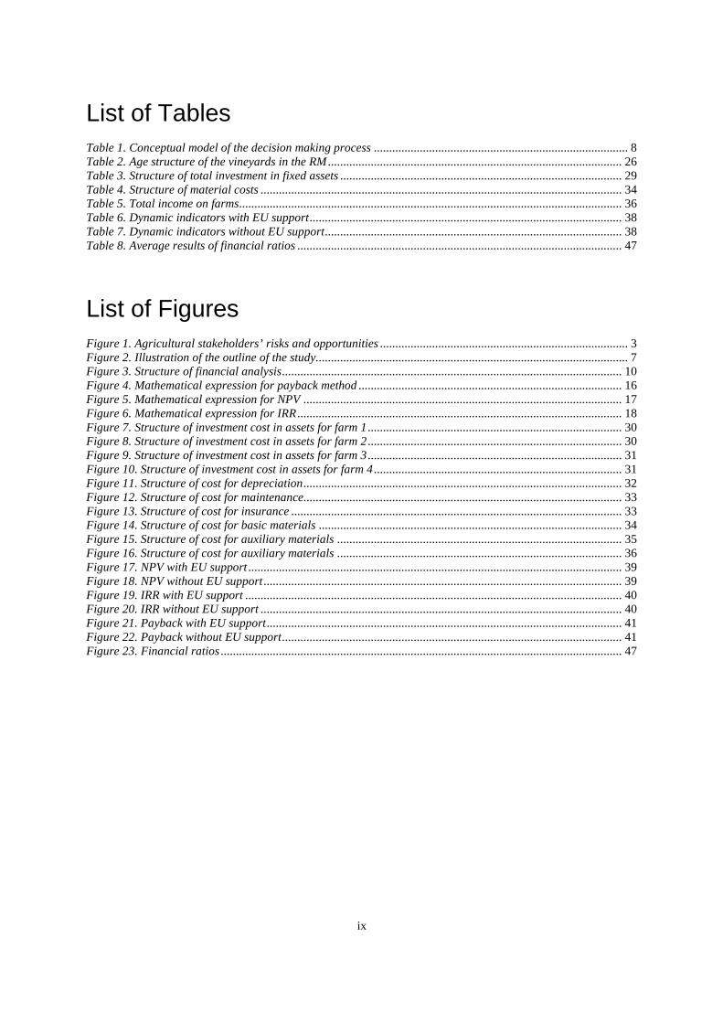
List of Tables Table 1. Conceptual model of the decision making process ................................................................................... 8 Table 2. Age structure of the vineyards in the RM ................................................................................................ 26 Table 3. Structure of total investment in fixed assets ............................................................................................ 29 Table 4. Structure of material costs ...................................................................................................................... 34 Table 5. Total income on farms ............................................................................................................................. 36 Table 6. Dynamic indicators with EU support ...................................................................................................... 38 Table 7. Dynamic indicators without EU support ................................................................................................. 38 Table 8. Average results of financial ratios .......................................................................................................... 47

List of Figures Figure 1. Agricultural stakeholders’ risks and opportunities ................................................................................. 3 Figure 2. Illustration of the outline of the study...................................................................................................... 7 Figure 3. Structure of financial analysis ............................................................................................................... 10 Figure 4. Mathematical expression for payback method ...................................................................................... 16 Figure 5. Mathematical expression for NPV ........................................................................................................ 17 Figure 6. Mathematical expression for IRR .......................................................................................................... 18 Figure 7. Structure of investment cost in assets for farm 1 ................................................................................... 30 Figure 8. Structure of investment cost in assets for farm 2 ................................................................................... 30 Figure 9. Structure of investment cost in assets for farm 3 ................................................................................... 31 Figure 10. Structure of investment cost in assets for farm 4 ................................................................................. 31 Figure 11. Structure of cost for depreciation ........................................................................................................ 32 Figure 12. Structure of cost for maintenance........................................................................................................ 33 Figure 13. Structure of cost for insurance ............................................................................................................ 33 Figure 14. Structure of cost for basic materials ................................................................................................... 34 Figure 15. Structure of cost for auxiliary materials ............................................................................................. 35 Figure 16. Structure of cost for auxiliary materials ............................................................................................. 36 Figure 17. NPV with EU support .......................................................................................................................... 39 Figure 18. NPV without EU support ..................................................................................................................... 39 Figure 19. IRR with EU support ........................................................................................................................... 40 Figure 20. IRR without EU support ...................................................................................................................... 40 Figure 21. Payback with EU support .................................................................................................................... 41 Figure 22. Payback without EU support ............................................................................................................... 41 Figure 23. Financial ratios ................................................................................................................................... 47

x

1

1 Introduction The investment is the investment of funds in the purchase and construction of real property to create conditions for a permanent business. On the farms there is a need for investment of new capital to enable to intensify production. To the economist the investment is a set of activities in investment capital for the production of economic benefits or to be more specific an investment is allocation of funds to assets used in production process which need to yield a gain, over some a period of time. As is usually comes to investing large amounts of cash with uncertain results, investment decisions are always risky business decisions. Therefore, an investor must take in consideration whether the expected results of the investments will be adequate. Farmers usually take lend for part of the required capital, and must provide evidence and others relevant proofs about the economic viability of investments. In addition, investment projects must be sufficiently profitable to the investor otherwise he may pay interest on loans and back-up capital invested during the life-cycle of the project. Thus the investment should provide maximum profit to the investor as a reward to the risk and responsibility in managing the new business. Traditional appraisal methods are best known technique’s ratings profitability of investment projects. This paper deals with the financial analysis in the field of decision making process, concerning economic profitability of investing in agricultural production, namely the fruit and grape production. The financial analysis method provide extremely useful information to the investor, since it makes possible to estimate the profitability of investment in incredibly specific conditions, by taking in to consideration numerous factors of it is economical efficiency as well as the main effects that can be expected. So, it can be said that financial analysis provides necessary information for the business itself and what kind of decisions need to be taken. So, if a comparison between a farmer and a financial manager is made, it can be said that they are the same because “The primary role of the financial manager is to ensure that his or her company has a sufficient supply of capital. The financial manager is at the crossroads of the real economy, with its industries and services, and the world of finance, with its various financial markets and structures.” Vernimmen et. al (2009) In today’s economies, business planning has become a very important tool which provides realistic information of choice for analysing data and management tool for developing strategies. 1.1 Problem background The RM (see Appendix 1) covers an area of 25.713 km 2. Half of that area or approximately 50% is an agricultural land or 1.275.000 ha (Ministry of Agriculture, Forestry and Water Economy (MAFWE), Annual Agricultural and Rural Development Report, 2009). The land is characterized with fertile soil and favourable climate, which is a good condition for agricultural development. So, under natural conditions favourable for agricultural production, it is reasonable to expect that the agricultural sector support and recovery and encourage the further development of the country.

2

The agricultural sector is the third largest sector according to the share in gross domestic product (GDP) and plays an important role in the Macedonian economy because it contributes to the national economy (GDP) by 9.7% (MAFWE, Annual Agricultural and Rural Development Report, 2009). It is characterized by a large number of small and heterogenic holdings. According to the preliminary data from the 2007 Agricultural Census, 192 378 agricultural holdings, cultivate 264 338 ha. According to the same source, the average Macedonian farm utilises agricultural area of as low as 1.37 ha (87.5% of all holdings cultivate less than 10 ha of utilised agricultural area). More than 80% of the land is owned or rented by family farms (State Statistical Office (SSO), (2008). Fruit production is the most successful sub-sector within the Macedonian agriculture sector. On approximately 35,000 ha (orchards and vineyards) more than 437,440.00 tonnes of fruits (grapes, apples, plums, apricots, pears, etc.) are produced. Of all fruits which are produced on Macedonian soil, grapes are produced on 19 960 ha with 253, 456.00 tonnes and orchards are disseminate on 14.000 ha with an annual production of 183,984.00 tonnes (SSO, 2010). Nowadays the agricultural sector is facing difficulties with its competitiveness as a result of low or insignificant investments in production technology, difficulties in providing loans, and small size farms (National Agricultural and Rural Development Programme (NARDS) 2007-2013). The Macedonian vegetables production sub-sector is facing the poor capital endowments (investment and working capital), poor access to credit, inadequate public investment financial support in particular for multi-annual crops and installations (greenhouses, post-harvest facilities), old farm machinery, often inadequate or having low quality planting material and outdated farming practices (little updated plantations, inappropriate use of agricultural inputs, lack of drip irrigation systems, etc), which is reflected in fluctuating and low yields. But the largest problem is low investments in multi-annual crops (leads to obsolescence of fruit and grape plantations) (NARDS 2007-2013). In 1991, the RM gained its independence and started the process of economic development. Agriculture suffered many changes in the process of transition and faced many difficulties to adjust to the new standards of production and the newly conditions which were set by the international market. As a result, in order to fulfill the European Union (EU) requirements, many farmers were faced with problems in order to adjust to these transformations. One of the many reasons for this was lack of information and knowledge. Nowdays the RM is in the process of acquiring a full membership of the EU, hence the RM being eligible for the pre-accession assistance through establishment of an Instrument for Pre-accession Assistance (IPA) in accordance with EC Regulation 1085/2006 of 17th of July. Under the IPA’s fifth component for rural development (IPARD), the country is entitled for a pre-accession financial aid for sustainable agriculture and rural development. The main focus is put towards preparing for the Common Agricultural Policy (CAP) and related policies and for the European Agricultural Fund for Rural Development, as well as for adjusting the sector towards the Common Market. The main purpose of this Program is to improve the agricultural sector in the country by helping farmers to reach acceptable standards of living and working conditions, improving the quality of production as well as farming profitability and to improve the processing and marketing conditions for agricultural products in order to fulfill the EU requirements (IPARD Programme 2007-2013, 2007). Small Enterprise Assistance Funds (SEAF) in Miler et. al, 2010 illustrates (see figure 1) the risks and the opportunities for agribusiness investment.

3

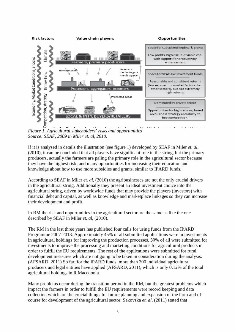
Figure 1. Agricultural stakeholders’ risks and opportunities Source: SEAF, 2009 in Miler et. al, 2010. If it is analysed in details the illustration (see figure 1) developed by SEAF in Miler et. al, (2010), it can be concluded that all players have significant role in the string, but the primary producers, actually the farmers are paling the primary role in the agricultural sector because they have the highest risk, and many opportunities for increasing their education and knowledge about how to use more subsidies and grants, similar to IPARD funds. According to SEAF in Miler et. al, (2010) the agribusinesses are not the only crucial drivers in the agricultural string. Additionally they present an ideal investment choice into the agricultural string, driven by worldwide funds that may provide the players (investors) with financial debt and capital, as well as knowledge and marketplace linkages so they can increase their development and profit. In RM the risk and opportunities in the agricultural sector are the same as like the one described by SEAF in Miler et. al, (2010). The RM in the last three years has published four calls for using funds from the IPARD Programme 2007-2013. Approximately 45% of all submitted applications were in investments in agricultural holdings for improving the production processes, 30% of all were submitted for investments to improve the processing and marketing conditions for agricultural products in order to fulfill the EU requirements. The rest of the applications were submitted for rural development measures which are not going to be taken in consideration during the analysis. (AFSARD, 2011) So far, for the IPARD funds, more than 300 individual agricultural producers and legal entities have applied (AFSARD, 2011), which is only 0.12% of the total agricultural holdings in R.Macedonia. Many problems occur during the transition period in the RM, but the greatest problems which impact the farmers in order to fulfill the EU requirements were record keeping and data collection which are the crucial things for future planning and expansion of the farm and of course for development of the agricultural sector. Sekovska et. al, (2011) stated that

4

“inconvenient and late privatization in agro complex, still influence in a negative way on agricultural development”. Data collection and record keeping as mentioned before are crucial parts of farm management and unfortunately are not practice by the Macedonian farmers. If a functional farm accountancy data system would be developed that could be useful for the decision-makers in creating adequate agricultural policy, also in validation of the results from the appropriate measures and the integration effects. In addition, it can support the advisory and extension segment, as well as the study and academic community (Martinovska-Stojceska et. al, 2009). Now in the RM, many workshops and training programmes are organized in order to educate the individual agricultural producers and legal entities.1

1.2 Problem According to the Law for Agriculture and rural development (2010), “an agricultural production (agricultural activities) is an economic activity involving the cultivation of annual crops, cultivation of perennial plants, growing plants for seed and planting material, animal husbandry and poultry, mixed agricultural activities and ancillary activities for agriculture and post-harvest activities, except veterinary and phytosanitary services in accordance with the regulations for statistical classification of economic activities in Macedonia”. In the last few years, the agricultural sector in Macedonia was revealed to important functional and lawful reforms. These reforms were done especially in the development of conformity of the national legislation, i.e. increase of the institutional organization according to EU standards, in the sectors managed by CAP. The EU assimilation processes are basic for increasing and establishing a viable agricultural sector in accordance with EU standards. In this way, MAFWE has presented some principles, procedures and mechanisms for realisation of the establishment and improvement processes in 86 agricultural production and markets, agricultural principles, rural development, budgetary support of the agricultural development and rural areas (Government of the RM, 2009). In recent years new techniques of agricultural investment assessment has occurred in order to maximize the profit and wealth of the business. Understandings these new techniques are important to a manager/farmer because they can help them make better investment decisions. In addition, the rapid evolution of Informational and Comunnicational Technologies has significant potential upon farming and offers agricultural extension services with a new array of channels and opportunities for information dissemination, thus tentatively replacing traditional modes of information delivery (Michailidis et. al, 2001). The development of new

1“Agricultural producer is the holder of the farm or a family farm or a person permanently or temporarily employed in the agricultural economy and which is engaged in agricultural activity”. (www, Law for Agriculture and rural development, 2010). “Farm is an economic unit under single management (from one or more persons regardless of ownership, legal form, size or location) whose agricultural property (who owns and/or disposal) shall be made for agricultural activity and which are recorded in Ministry of Agriculture, Forestry and Water Management (hereinafter: Ministry). Agriculture includes one or more production units. Farm can be legally organized as a trading company or other entity established by law or family farm”. (www, Law for Agriculture and rural development, 2010). “Family agricultural household is an independent economic and social unit that is based on a combination of management and ownership and/or use of agricultural property from family members” (www, Law for Agriculture and rural development, 2010). “Holder of the family agricultural household is an adult who is responsible for managing the agricultural economy and that acting on behalf of the family farm and as such is only recorded in the Farm Register in Ministry. Holder of the farm which is legally organized as a trading company or other entity established by law is itself a legal person, the person in charge of the legal person acting on behalf of farm” (www, Law for Agriculture and rural development, 2010).

5

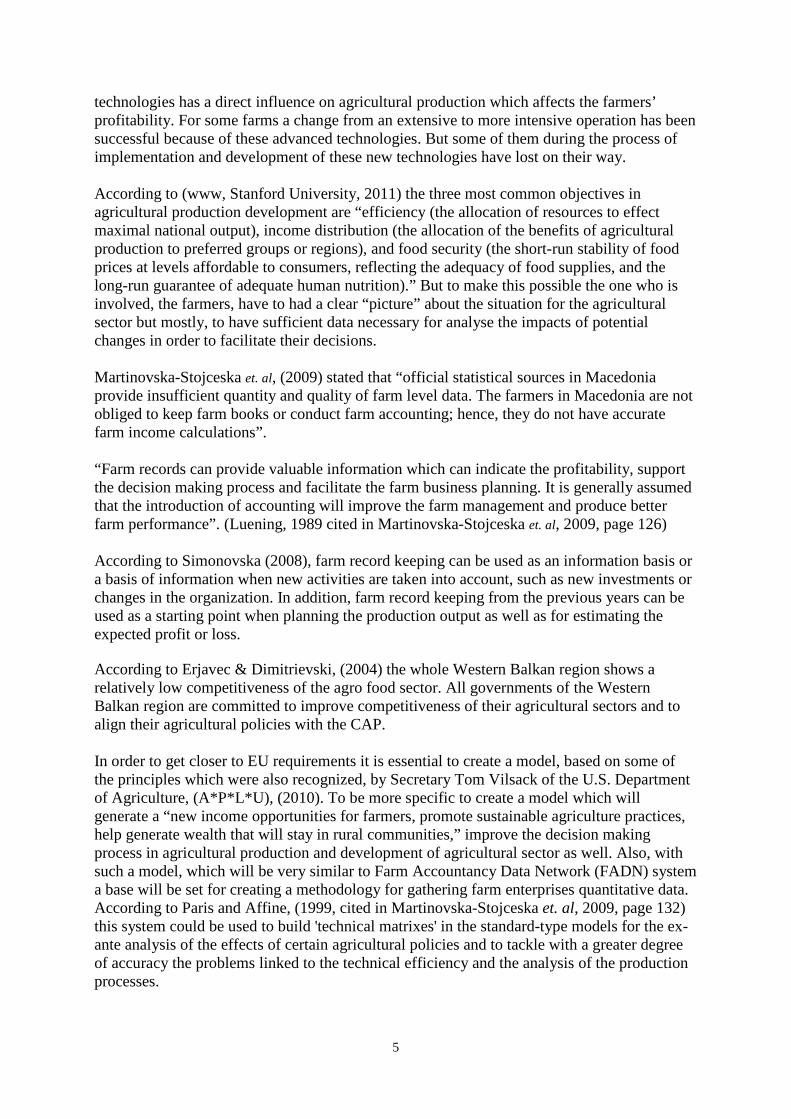
technologies has a direct influence on agricultural production which affects the farmers’ profitability. For some farms a change from an extensive to more intensive operation has been successful because of these advanced technologies. But some of them during the process of implementation and development of these new technologies have lost on their way. According to (www, Stanford University, 2011) the three most common objectives in agricultural production development are “efficiency (the allocation of resources to effect maximal national output), income distribution (the allocation of the benefits of agricultural production to preferred groups or regions), and food security (the short-run stability of food prices at levels affordable to consumers, reflecting the adequacy of food supplies, and the long-run guarantee of adequate human nutrition).” But to make this possible the one who is involved, the farmers, have to had a clear “picture” about the situation for the agricultural sector but mostly, to have sufficient data necessary for analyse the impacts of potential changes in order to facilitate their decisions. Martinovska-Stojceska et. al, (2009) stated that “official statistical sources in Macedonia provide insufficient quantity and quality of farm level data. The farmers in Macedonia are not obliged to keep farm books or conduct farm accounting; hence, they do not have accurate farm income calculations”. “Farm records can provide valuable information which can indicate the profitability, support the decision making process and facilitate the farm business planning. It is generally assumed that the introduction of accounting will improve the farm management and produce better farm performance”. (Luening, 1989 cited in Martinovska-Stojceska et. al, 2009, page 126) According to Simonovska (2008), farm record keeping can be used as an information basis or a basis of information when new activities are taken into account, such as new investments or changes in the organization. In addition, farm record keeping from the previous years can be used as a starting point when planning the production output as well as for estimating the expected profit or loss. According to Erjavec & Dimitrievski, (2004) the whole Western Balkan region shows a relatively low competitiveness of the agro food sector. All governments of the Western Balkan region are committed to improve competitiveness of their agricultural sectors and to align their agricultural policies with the CAP. In order to get closer to EU requirements it is essential to create a model, based on some of the principles which were also recognized, by Secretary Tom Vilsack of the U.S. Department of Agriculture, (A*P*L*U), (2010). To be more specific to create a model which will generate a “new income opportunities for farmers, promote sustainable agriculture practices, help generate wealth that will stay in rural communities,” improve the decision making process in agricultural production and development of agricultural sector as well. Also, with such a model, which will be very similar to Farm Accountancy Data Network (FADN) system a base will be set for creating a methodology for gathering farm enterprises quantitative data. According to Paris and Affine, (1999, cited in Martinovska-Stojceska et. al, 2009, page 132) this system could be used to build 'technical matrixes' in the standard-type models for the ex-ante analysis of the effects of certain agricultural policies and to tackle with a greater degree of accuracy the problems linked to the technical efficiency and the analysis of the production processes.

6

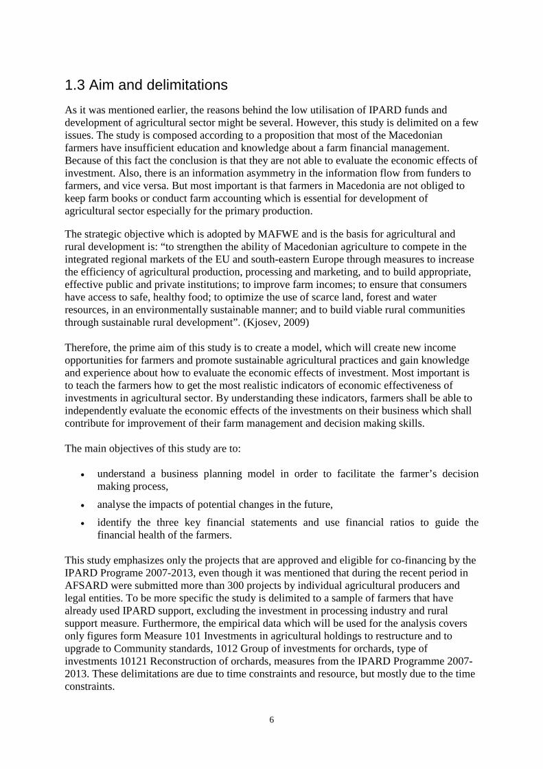
1.3 Aim and delimitations As it was mentioned earlier, the reasons behind the low utilisation of IPARD funds and development of agricultural sector might be several. However, this study is delimited on a few issues. The study is composed according to a proposition that most of the Macedonian farmers have insufficient education and knowledge about a farm financial management. Because of this fact the conclusion is that they are not able to evaluate the economic effects of investment. Also, there is an information asymmetry in the information flow from funders to farmers, and vice versa. But most important is that farmers in Macedonia are not obliged to keep farm books or conduct farm accounting which is essential for development of agricultural sector especially for the primary production. The strategic objective which is adopted by MAFWE and is the basis for agricultural and rural development is: “to strengthen the ability of Macedonian agriculture to compete in the integrated regional markets of the EU and south-eastern Europe through measures to increase the efficiency of agricultural production, processing and marketing, and to build appropriate, effective public and private institutions; to improve farm incomes; to ensure that consumers have access to safe, healthy food; to optimize the use of scarce land, forest and water resources, in an environmentally sustainable manner; and to build viable rural communities through sustainable rural development”. (Kjosev, 2009) Therefore, the prime aim of this study is to create a model, which will create new income opportunities for farmers and promote sustainable agricultural practices and gain knowledge and experience about how to evaluate the economic effects of investment. Most important is to teach the farmers how to get the most realistic indicators of economic effectiveness of investments in agricultural sector. By understanding these indicators, farmers shall be able to independently evaluate the economic effects of the investments on their business which shall contribute for improvement of their farm management and decision making skills. The main objectives of this study are to:

• understand a business planning model in order to facilitate the farmer’s decision making process,

• analyse the impacts of potential changes in the future, • identify the three key financial statements and use financial ratios to guide the

financial health of the farmers. This study emphasizes only the projects that are approved and eligible for co-financing by the IPARD Programe 2007-2013, even though it was mentioned that during the recent period in AFSARD were submitted more than 300 projects by individual agricultural producers and legal entities. To be more specific the study is delimited to a sample of farmers that have already used IPARD support, excluding the investment in processing industry and rural support measure. Furthermore, the empirical data which will be used for the analysis covers only figures form Measure 101 Investments in agricultural holdings to restructure and to upgrade to Community standards, 1012 Group of investments for orchards, type of investments 10121 Reconstruction of orchards, measures from the IPARD Programme 2007-2013. These delimitations are due to time constraints and resource, but mostly due to the time constraints.

7

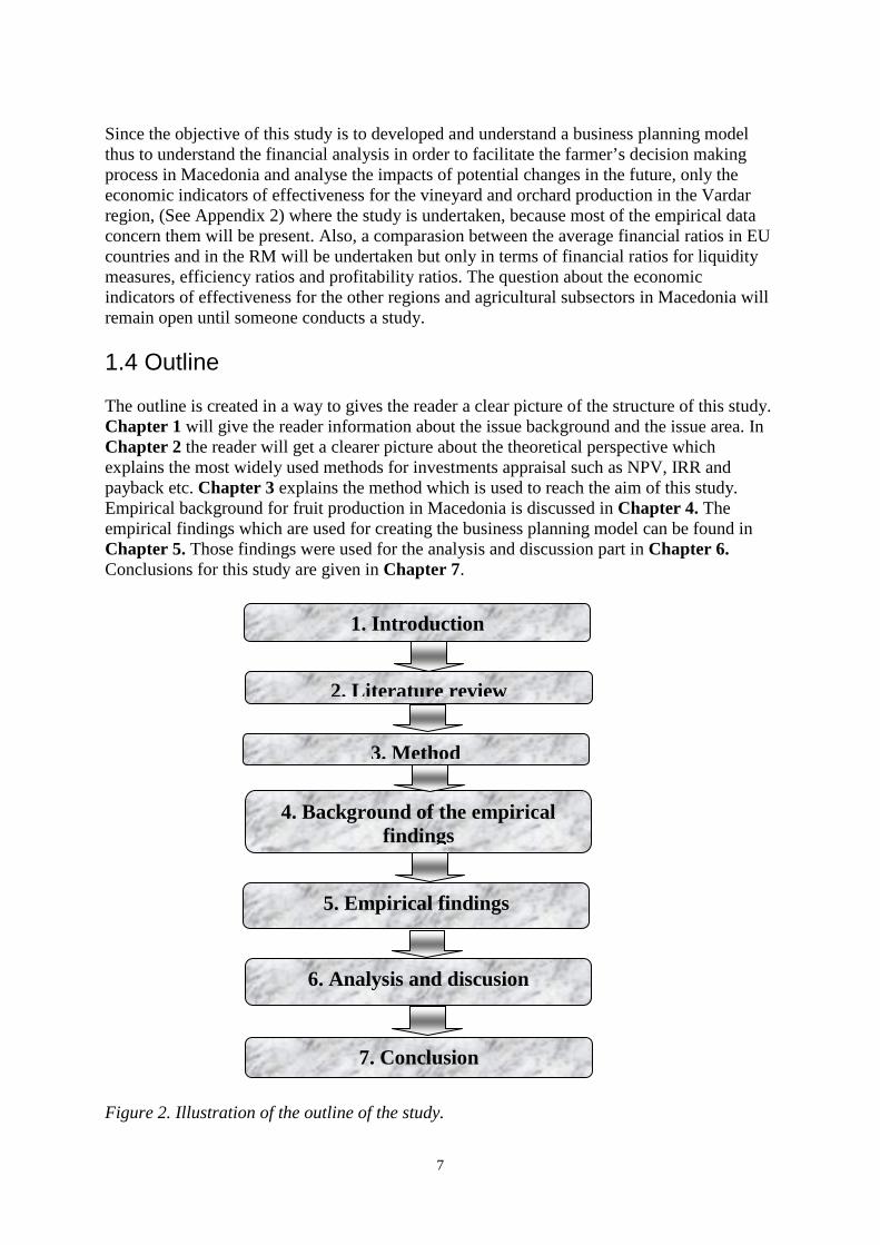
Since the objective of this study is to developed and understand a business planning model thus to understand the financial analysis in order to facilitate the farmer’s decision making process in Macedonia and analyse the impacts of potential changes in the future, only the economic indicators of effectiveness for the vineyard and orchard production in the Vardar region, (See Appendix 2) where the study is undertaken, because most of the empirical data concern them will be present. Also, a comparasion between the average financial ratios in EU countries and in the RM will be undertaken but only in terms of financial ratios for liquidity measures, efficiency ratios and profitability ratios. The question about the economic indicators of effectiveness for the other regions and agricultural subsectors in Macedonia will remain open until someone conducts a study. 1.4 Outline The outline is created in a way to gives the reader a clear picture of the structure of this study. Chapter 1 will give the reader information about the issue background and the issue area. In Chapter 2 the reader will get a clearer picture about the theoretical perspective which explains the most widely used methods for investments appraisal such as NPV, IRR and payback etc. Chapter 3 explains the method which is used to reach the aim of this study. Empirical background for fruit production in Macedonia is discussed in Chapter 4. The empirical findings which are used for creating the business planning model can be found in Chapter 5. Those findings were used for the analysis and discussion part in Chapter 6. Conclusions for this study are given in Chapter 7.

Figure 2. Illustration of the outline of the study.

6. Analysis and discusion

7. Conclusion

5. Empirical findings

4. Background of the empirical findings

3. Method

2. Literature review

1. Introduction

8

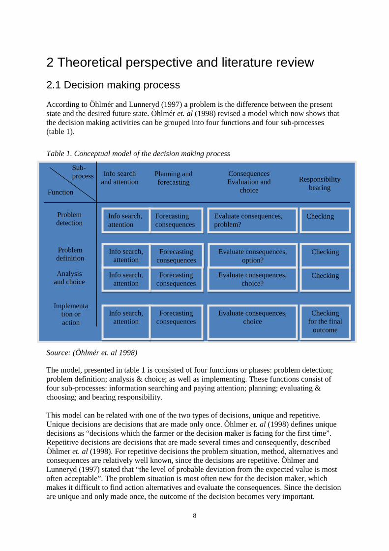
2 Theoretical perspective and literature review 2.1 Decision making process According to Öhlmér and Lunneryd (1997) a problem is the difference between the present state and the desired future state. Öhlmér et. al (1998) revised a model which now shows that the decision making activities can be grouped into four functions and four sub-processes (table 1).

Table 1. Conceptual model of the decision making process

Source: (Öhlmér et. al 1998)

The model, presented in table 1 is consisted of four functions or phases: problem detection; problem definition; analysis & choice; as well as implementing. These functions consist of four sub-processes: information searching and paying attention; planning; evaluating & choosing; and bearing responsibility. This model can be related with one of the two types of decisions, unique and repetitive. Unique decisions are decisions that are made only once. Öhlmer et. al (1998) defines unique decisions as “decisions which the farmer or the decision maker is facing for the first time”. Repetitive decisions are decisions that are made several times and consequently, described Öhlmer et. al (1998). For repetitive decisions the problem situation, method, alternatives and consequences are relatively well known, since the decisions are repetitive. Öhlmer and Lunneryd (1997) stated that “the level of probable deviation from the expected value is most often acceptable”. The problem situation is most often new for the decision maker, which makes it difficult to find action alternatives and evaluate the consequences. Since the decision are unique and only made once, the outcome of the decision becomes very important.

Planning and forecasting

Info search and attention

Consequences Evaluation and

choice Responsibility

bearing

Problem detection

Problem definition

Analysis and choice

Implementation or action

Function

Sub-process

Forecasting consequences

Forecasting consequences

Forecasting consequences

Forecasting consequences

Evaluate consequences, problem?

Evaluate consequences, option?

Evaluate consequences, choice?

Evaluate consequences, choice

Checking

Checking

Checking

Checking for the final

outcome

Info search, attention

Info search, attention

Info search, attention

Info search, attention

9

Most farmers in Macedonia are facing with unique decisions because they are facing with the EU grand’s for the first time. That is why it is essential for them to explain the benefits of investing, even if they do not use a financial grant. The first sub-process of the model presented above in table 1, which is information searching and paying attention, is essential for understanding a business planning in order to facilitate the farmer’s decision making process. When you have all the necessary information it is easy to plan, evaluate & choose and bearing the responsibility by the decision. The information’s which are needed for this are hidden somewhere in the financial analysis of investments. 2.2 Financial analysis Today the system of values of business subjects is being transformed into general objectives of an enterprise (economic, financial, social, environmental and others) which are mainly implemented with the help of investment projects (Bhat and Rau, 2008). Therefore, the efficiency of investment projects is evaluated by using economic, financial, technological, ecological-environmental and other efficiency indicators. However, in practice sometimes it is difficult to make investment decisions as often, according to some of these indicators, an investment project can be very beneficial and efficient, while according to other factors it can even be inappropriate to implement. It is also common that one efficiency indicator is picked out of the context and decisions are based on it. According to same authors the evaluation is also hampered by the fact that it is necessary to take into account the importance of individual indicators (i.e. indicators are not of equal importance) in order to achieve the investment targets. According to Radu and Dimitru (2011), there is no one specific generalized indicator to cover all aspects of investment project analysis and to show the general (integrated) efficiency of a project, as the impact of different factors on a project is of diverse origin and they are targeted to evaluate different investment objectives. As I mentioned before this paper consider the viability of investments in agriculture based on contemporary financial analysis. The analysis allows the assessment of relative profitability investment in the proposed projects. Methods of analysis examine costs, benefits and risks of all options to determine cost-effective ways of achieving the goals. According to Fabozzi & Peterson (2003), а finance is the application of economic principles and concepts to business decision making and problem solving. The field of finance can be considered to comprise three broad categories: financial management, investments and financial institutions. The same authors stated that the financial management encompasses many different types of decisions, such as investment decisions, financing decisions, and decisions that involve both investing and financing. As mentioned before, according to Vernimmen et. al (2009), “the primary role of the financial manager is to ensure that his or her company has a sufficient supply of capital. The financial manager is at the crossroads of the real economy, with its industries and services, and the world of finance, with its various financial markets and structures”. Hence a farmer should be similar to what a financial manager of a large corporation is. The financial analysis in broadest sense is analysis that has to do with budgets and finances over time. Within the analysis of the operation is perceived risk and return in order to make better decisions about investing or lending. Such analysis indicated the ability to see into the future,

10

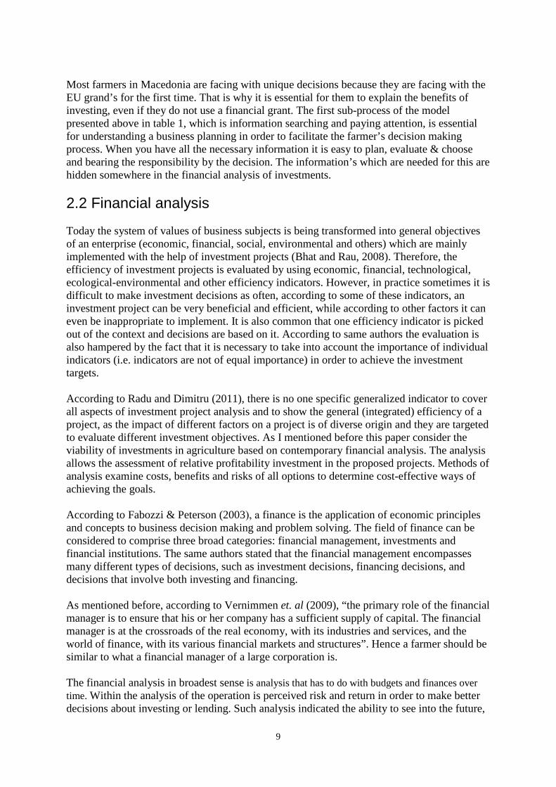
and it is therefore necessary to explain the past and provide a basis for projecting future earnings. Hence, financial analysis is a tool of financial management (Fabozzi & Peterson, 2003). In figure 3 a structure of a financial analysis is presented.

Figure 3. Structure of financial analysis Source: Florio, M, Ugo F, et. al, 1997 According to Florio, M, Ugo F, et. al, (1997) “the purpose of the financial analysis is to use the project’s cash flow forecasts in order to calculate suitable return rates, specifically the financial internal rate of return (FRR) on investment (FRR/C) and own capital (FRR/K) and the corresponding financial net present value (FNPV)”. In order to carry out the financial analysis first, a determination of total costs need to be found, and then to calculate suitable return rates. Figure 3, describes the structure of financial analysis. Financial analysis shows the efficiency and effectiveness of financial policy, as one of the essential elements in managing the finances of the company. Results of financial analysis are important for establishing appropriate financial strategy of the farm. To understand the firm’s performance, financial managers use the information contained in the financial statements. The main objective of financial analysis is the perception of weakness that can lead to financial problems of the company and take adequate measures for their elimination in the future. Financial analysis should provide answers on how the company's liquidity, as management financed investments, whether the company achieves sufficient amount of profit, whether shareholders receive sufficient funds on the basis of ownership. Financial analysis is the financial calculations on which the financial analysis, namely the balance sheet, income success and report on the financial condition flows. Balance report on the financial position of enterprises on a particular day represents "image" the company's assets at some point. Balance shows the success of the business success of companies in a given period of time. Financial analysis can be realised by applying different methods, of which the most significant are visual analysis, using account coverage, analysis using the net working fund, cash flow analysis, funds flow analysis and ratio analysis. Rational analysis is the most complex approach to determining the creditworthiness of companies, because it most directly demonstrates the ability of the agreed loan repayment obligations, the level of efficient operation and utilisation of resources, the level of the operational use of available resources, the ability of participation and self-financing and overall business performance of companies of which depends on repayment capacity, efficient use of credit resources and the level of potential credit risk. (Florio, M, Ugo F, et. al, 1997)

11

In order to carry out a reliable analysis of business enterprises, it is necessary to ensure accuracy of the information, and it is necessary that accounting and other operational data be prepared and presented in accordance with the current economic - financial regulations and be correct and objective. It is also necessary uniformity of data, also methods used to obtain data on business enterprises to be upfront determined and that can not be changed according to current needs. By undisputed used in analysing financial statements, ratio analysis has certain restrictions. This analysis is favourable for small and medium enterprises, and unfavourable for analysis of multinational companies. It cannot be "supplied inserted" the impact of inflation or disinflation, due to the application principles of historical cost. It is difficult to generalize whether a ratio of "good" or "bad", since it depends on the type of company and of the areas in which the firm operates. (Pike & Neale, 2006) Financial analysis is the process of establishing relations between the factors that, in this case related to the determination of financial position and activities of the company. Therefore, the object of analysis is the firm that is its financial position, whose significance is best seen from the fact that the financial position of crucial importance to business success, and thus in what is today a huge competitive conditions also matter-market survival. The meaning of the existence of any undertaking, whether it provides services or products is that all entities within it to satisfy their needs (employees) and those from the environment meet the needs of just what the company offers them (consumers). Financial analysis is based on data that include balance sheet and profit and loss success. It is therefore very important that these data are accurate and complete. Reason why the rational numbers are calculated in financial analysis is that the balance sheet positions are of little analytical value. Rational numbers are obtained by placing a relative position of certain balance sheet and success. Information from financial analysis represents the basis for taking action is aimed at improving the creditworthiness of the trend of growth and development of business enterprises. The subjects of the analysis are the means and resources (data obtained from balance sheet) and operating results or business income and expenses (this information taken from the balance of success). Balance of success, as the end result, given the difference between money earned and spent then profit or loss. There is in general terms give a cost (direct labor, materials, etc.) Operating expenses (sales, marketing, administration, etc.), as well as income. If a business plan is projected for more than one year, the balance of success must be displayed for each year. (Fabozzi & Petterson, 2003) 2.2.1 Financial statements According to Vernimmen et. al (2009), a firm financial health is summarized in three key financial reports: (1) the income statement, (2) the balance sheet, and (3) the cash flow statement. These reports summarize detailed information on a firm’s financial actions during the preceding fiscal year and its financial position at the end. Annual statements cover one year periods ending at a specified date. For most firms and farms, the ending date is the end of the calendar year. Many large corporations, however, operate on 12-month cycles (or fiscal years) that end at times other than December 31. In addition to annual reports to stockholders, corporations usually prepare monthly statements to guide a corporation’s executives, as well as quarterly statements that must be made available to stockholders of publicly held corporations. Financial statements are based on values from a farm’s cost accounting system (Clauss J, 2010).

12

In RM the statements follow the International Financial Reporting Standards (IFRS) adopted by the International Accounting Standards Board (IASB) in order for standalone/separate and consolidated financial statements. According (www.pwc.com, 2011) “an update on the IFRS was published in the Official Gazette in 2009, effective from January 1, 2010 (harmonized with IASB). However, IFRS 9, as well as certain IFRICs (IFRIC 18 and IFRIC 19) have not been published in the Official Gazette and, therefore, are not yet applicable in Macedonia.” 2.2.2 The income statement The income statements provide a financial summary of a firm’s operation for a specified period, such as one year ending at the date specified in the statement’s title. They show the total revenues and expenses during that time. An income statement is sometimes called a “profit and loss statement,” an “operating statement,” or a “statement of operations.” Essentially, it tells whether or not the firm is making money. Certain items, such as depreciation, are an expense although they do not involve a cash outlay. Some items, such as the sale of goods or services, are recognized as income even though buyers have not yet paid for them. Other items, such as purchased materials, are recognized as expenses even though the firm has not yet paid for them. Such income and expense items are recorded when they are accrued (e.g., when sold goods are shipped), not when cash actually flows. (Brigham & Ehrhardt, 2010) Annual income statements for large corporations are organized in the same format according to the IFRS. The income statement is organized into several sections. The upper section reports the firm’s revenues and expenses from its principal operations. Below that are nonoperating items, such as financing costs (e.g., interest expense) and taxes. (Brigham & Ehrhardt, 2010) 2.2.2.1 The Items on an Income Statement Total operating revenue (or total sales revenues) is the income earned from the firm’s operations during the fiscal year reported. The cost of goods sold for a retail firm is the amount paid to wholesalers or other suppliers for the goods that the firm resells to its customers. The cost of goods sold for a factory includes the cost of direct production labor and materials used to manufacture the goods. Gross profit is the amount left after paying for the goods that were sold. Operating expenses are those that are the cost of a firm’s day-to-day operations rather than a direct cost for making a product. Selling expenses are the costs for marketing and selling the company’s products, such as advertising costs and the salaries and commissions paid to sales personnel. General and administrative expenses include the salaries of the firm’s officers and other management personnel and other costs that are included in the firm’s administrative expenses (e.g., legal and accounting expenses, office supplies, travel and entertainment, insurance, telephone service, and utilities). Fixed Expenses include such costs as the leasing of facilities or equipment. (Beringa, 2005) Depreciation expenses are the amount by which the firm reduced the book value of its capital assets during the preceding year. Total operating expense is the sum of the individual expenses. Net operating income (also called net operating profit) is what is left after subtracting the total operating expense from the gross profits. Other income is income derived from nonoperating sources. Earnings before interest and taxes (EBIT) are the difference between income and the sum of the operating expenses. Interest expense is the cost paid for

13

borrowing funds. Interest on short-term notes is that paid on loans from banks or commercial notes that the company issues for short terms, such as 30 days to 90 days, in order to meet payrolls and other current obligations during months when expenses exceed income. (The company may also earn interest by lending excess funds to others during periods when its income exceeds expenses.) Interest on long-term borrowing is that paid on bonds or other multiyear debts that the company incurs in order to raise capital for capital assets, such as factories and other facilities. Taxes are computed by multiplying EBT by the tax rate. Earnings after taxes (EAT, also known as the net profits (or earnings after taxes) are what are left after subtracting taxes from EBT. (Bhat and Rau, 2008) 2.2.3 Balance sheet According Beringa (2005), the balance sheets summarize a firm’s assets, liabilities, and equity at a specific point in time. Assets are anything a firm owns, both tangible and intangible, that has monetary value. Liabilities are the firm’s debts, or the claims of creditors against a firm’s assets. Equity (also called stockholders’ equity or net worth) is the difference between total assets and total liabilities. In principle, equity is what should remain for holders of common and preferred stock after a company discharges its obligations. As every introductory course in accounting or financial management teaches, the fundamental relationship for balancing the balance sheet is:

Total Assets = Liabilities + Net Worth Balance sheet accounting view "left and right." On the left side of the table are usually shown in the asset and liabilities on the right. The left and right sides as the final result, i.e. the sum of all counts, they must have the same figure. If not, it is a sign that a wrong calculation is made. The assets include cash and receivables, as well as property and fixed assets, inventories, and possible losses. Duties include all current and future payments, loans, core capital and retained earnings. The balance sheet is also true for each year in the business plan. (Helfred, 2001) 2.2.3.1 The Items on a Balance sheet Assets are generally listed according to the length of time that would take an ongoing firm to convert them to cash. They are separate as current assets, fixed assets and total assets. Current assets include cash and other items, such as marketable securities, that the company can or expects to convert to cash in the near future that is, in less than a year. Cash, as the name suggests, includes both money on-hand and in bank deposits. Marketable securities are short-term, interest-bearing, money-market securities that are issued by the government, businesses, and financial institutions. Firms purchase them to obtain a return on temporarily idle funds. Cash and marketable securities are often lumped together as a single item called “Cash and equivalents. Accounts receivable is the amount of credit extended by a firm to its customers. When payments are not received within 90 days, the amounts due are generally put into a separate account for bad debt. Inventories include supplies, raw materials, and components used for manufacturing products: work in-process. (Bhat and Rau, 2008) Fixed assets are tangible and intangible items that have long lives and are not readily convertible to cash. Fixed assets include such tangible items as land, buildings, equipment, furniture, and vehicles, and such intangible items as patents, trademarks, and goodwill. Total assets are the sum of the current and fixed assets. (Helfred, 2001)

14

Liabilities are also listed according to the length of time in which they are due. They are separated as current liabilities, long-term debt and total liabilities. Current liabilities are the sum of debts owed by the firm for which payment is due in the current year. Accounts payable is the amount the firm owes to others for goods or services purchased from them on credit. Short-term notes payable are outstanding short-term loans, typically from commercial banks. Long-term debt (or long-term liabilities) is the sum of debts owed by the firm for which repayment is not due in the current year. It generally includes various types of corporate bonds issued by the firm and long-term loans from banks that the firm has negotiated to raise funds for capital investments in facilities and other major projects. Total liabilities are the sum of the current and long-term liabilities. (Brigham & Ehrhardt, 2010) According the same author’s stockholders’ equity (also called shareholders’ equity or net worth) represents the owners’ claims on the firm. Retained earnings are the cumulative total of all earnings that has been kept in the firm since its inception. Balance sheets are so called because the sum of liabilities and net worth must equal the assets. That is:

Total Assets = Total Liabilities + Net Worth 2.2.4 The cash flow statement The authors Dimitriu and Caracota (2004) claim that the economic value of an investment, from the institution/organization’s point of view, is influenced by the investment project cash flows. There are three types of cash flows: initial investment costs, operating cash flows and cash flows at end of the project’s life. Different economic criteria are used in comparing financial investment alternatives, such as simple financial evaluation methods, which do not take into account the time value of money (static approach) or discount methods, that take into account the time factor (dynamic approach). Dynamic approaches are considered better as they include the time value of money and other important factors. According to Vasilescu (2009) and Vasilescu & Cicea (2004), the project’s economic evaluation requires economic efficiency computation and analysis, which corresponds to a causal relationship between the effort and the effect gained. A cash flow statement (or statement of cash flows) converts accounting data, which is used for creating the income statement and balance sheet, into a picture of cash inflows and outflows. That is, the cash flow statement shows where a firm’s money comes from and where it all goes. It identifies the amount generated by the firm and the amounts paid to the firm’s creditors and shareholders. The cash flow statement is the most conservative measure of a company’s financial health. Short of outright fraud, cash flow is much less vulnerable to “cooking the books” and creative accounting practices intended to make a company appear more attractive to investors. (Clauss J, 2010) A cash flow statement summarizes the inflows and outflows of funds during a specified period, typically the year just ended. The cash balance at the end of the reporting period is important information on the cash balance statement. It equals the cash balance at the beginning of the reporting period plus the cash inflows minus the cash outflows. The formula is: Ending cash balance = Beginning cash balance + Cash inflows (sources) – Cash outflows (uses)

15

2.2.4.1 Components of the Cash Flow Statement The cash flow statement generally divides cash flows into the following three components: (1) “cash flow from operations,” (2) “cash flow from changes in fixed assets” (also known as “cash flow from investing”), and (3) “cash flow from changes in net working capital” (also known as “cash flow from financing”). “Cash flow from operations” is generally a source of funds, or a net cash inflow. “Cash flow from changes in fixed assets” and “cash flow from changes in net working capital” are generally uses of funds, or cash outflows. The first of these two items describes the cash flows associated with changes in the firm’s mix of long-term fixed assets. The second describes cash flows associated with changes in financing the firm. (Beringa, 2005) 2.2.5 Financial Ratios In their study David A. et. al (2009) examined the techniques of ratios analysis. These ratios are examined thru comparisons of figures provided in the financial statements which are crucial to evaluate the financial status, performance and investment potential of a business. For evaluating the business performance, the return on total assets ratio (ROA) will be undertaken. As sub-analysis which will be carried out to determent the performance of a business, a net profit margin, gross profit margin and operating profit margin will be undertaken. All results are presented in Chapter 5. According to (Clauss J, 2010) “financial ratios are divided into the following six classes according to the types of information they provide and their uses:

1. Liquidity ratios, which describe a firm’s short-term solvency, or its ability to meet its current obligations

2. Activity and efficiency ratios, which describe how well a firm is using its investment in assets to produce sales and profits

3. Leverage or debt ratios, which describe to extent to which a firm relies on debt financing

4. Coverage ratios, which describe how well a firm is able to pay certain expenses 5. Profitability ratios, which describe how profitable a firm has been in relation to its

assets and shareholders’ equity 6. Stockholder and market value ratios, which describe the value of a firm in the eyes of

outside investors and security markets”.

For evaluating the financial status of the business, liquidity ratios such as: current and acid ratio will be used. For determining the solvency of the companies, the gearing ratio will be used and for determining the investment potential of a company can be used the net dividend, dividend cover ratio, price earnings ratio etc; but in this study, those evaluations will not be undertaken.

2.3 Investment appraisal methods In their study Lumby & Jones (2003), examined the traditional methods and the discounted methods of investment appraisal (payback, NPV and IRR) which will be taken in consideration for this study. Also, Vernimmen et. al (2009) examined the traditional methods

16

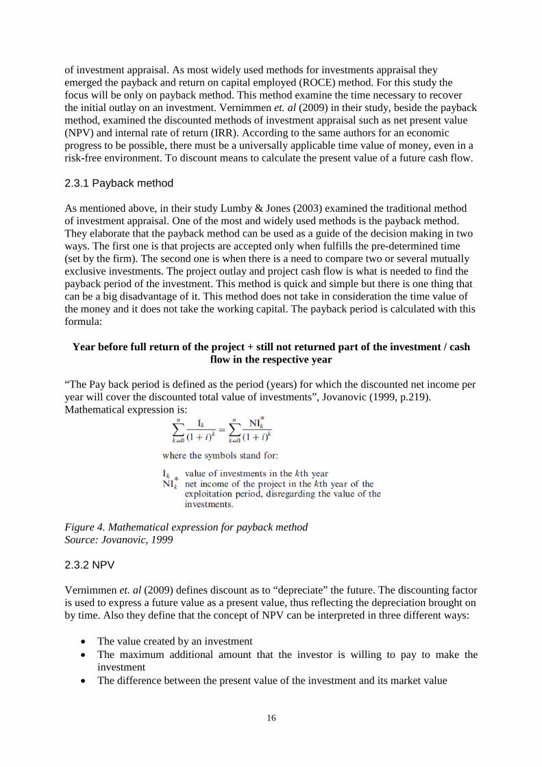
of investment appraisal. As most widely used methods for investments appraisal they emerged the payback and return on capital employed (ROCE) method. For this study the focus will be only on payback method. This method examine the time necessary to recover the initial outlay on an investment. Vernimmen et. al (2009) in their study, beside the payback method, examined the discounted methods of investment appraisal such as net present value (NPV) and internal rate of return (IRR). According to the same authors for an economic progress to be possible, there must be a universally applicable time value of money, even in a risk-free environment. To discount means to calculate the present value of a future cash flow. 2.3.1 Payback method As mentioned above, in their study Lumby & Jones (2003) examined the traditional method of investment appraisal. One of the most and widely used methods is the payback method. They elaborate that the payback method can be used as a guide of the decision making in two ways. The first one is that projects are accepted only when fulfills the pre-determined time (set by the firm). The second one is when there is a need to compare two or several mutually exclusive investments. The project outlay and project cash flow is what is needed to find the payback period of the investment. This method is quick and simple but there is one thing that can be a big disadvantage of it. This method does not take in consideration the time value of the money and it does not take the working capital. The payback period is calculated with this formula:

Year before full return of the project + still not returned part of the investment / cash flow in the respective year

“The Pay back period is defined as the period (years) for which the discounted net income per year will cover the discounted total value of investments”, Jovanovic (1999, p.219). Mathematical expression is:

Figure 4. Mathematical expression for payback method Source: Jovanovic, 1999 2.3.2 NPV Vernimmen et. al (2009) defines discount as to “depreciate” the future. The discounting factor is used to express a future value as a present value, thus reflecting the depreciation brought on by time. Also they define that the concept of NPV can be interpreted in three different ways:

• The value created by an investment • The maximum additional amount that the investor is willing to pay to make the

investment • The difference between the present value of the investment and its market value

17

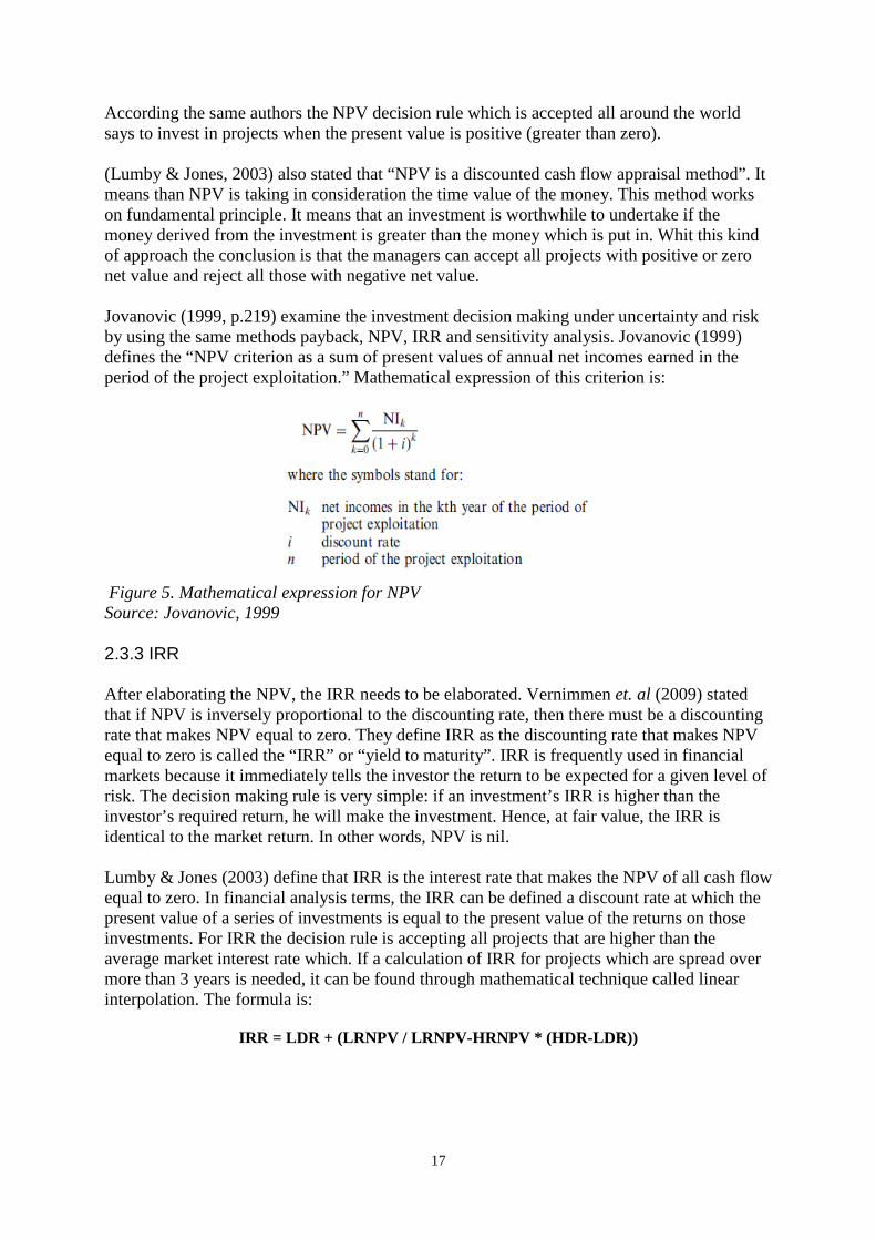
According the same authors the NPV decision rule which is accepted all around the world says to invest in projects when the present value is positive (greater than zero). (Lumby & Jones, 2003) also stated that “NPV is a discounted cash flow appraisal method”. It means than NPV is taking in consideration the time value of the money. This method works on fundamental principle. It means that an investment is worthwhile to undertake if the money derived from the investment is greater than the money which is put in. Whit this kind of approach the conclusion is that the managers can accept all projects with positive or zero net value and reject all those with negative net value. Jovanovic (1999, p.219) examine the investment decision making under uncertainty and risk by using the same methods payback, NPV, IRR and sensitivity analysis. Jovanovic (1999) defines the “NPV criterion as a sum of present values of annual net incomes earned in the period of the project exploitation.” Mathematical expression of this criterion is:

Figure 5. Mathematical expression for NPV Source: Jovanovic, 1999 2.3.3 IRR After elaborating the NPV, the IRR needs to be elaborated. Vernimmen et. al (2009) stated that if NPV is inversely proportional to the discounting rate, then there must be a discounting rate that makes NPV equal to zero. They define IRR as the discounting rate that makes NPV equal to zero is called the “IRR” or “yield to maturity”. IRR is frequently used in financial markets because it immediately tells the investor the return to be expected for a given level of risk. The decision making rule is very simple: if an investment’s IRR is higher than the investor’s required return, he will make the investment. Hence, at fair value, the IRR is identical to the market return. In other words, NPV is nil. Lumby & Jones (2003) define that IRR is the interest rate that makes the NPV of all cash flow equal to zero. In financial analysis terms, the IRR can be defined a discount rate at which the present value of a series of investments is equal to the present value of the returns on those investments. For IRR the decision rule is accepting all projects that are higher than the average market interest rate which. If a calculation of IRR for projects which are spread over more than 3 years is needed, it can be found through mathematical technique called linear interpolation. The formula is:

IRR = LDR + (LRNPV / LRNPV-HRNPV * (HDR-LDR))

18

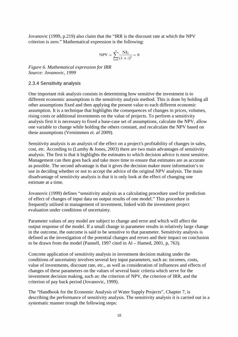
Jovanovic (1999, p.219) also claim that the “IRR is the discount rate at which the NPV criterion is zero.” Mathematical expression is the following:

Figure 6. Mathematical expression for IRR Source: Jovanovic, 1999

2.3.4 Sensitivity analysis

One important risk analysis consists in determining how sensitive the investment is to different economic assumptions is the sensitivity analysis method. This is done by holding all other assumptions fixed and then applying the present value to each different economic assumption. It is a technique that highlights the consequences of changes in prices, volumes, rising costs or additional investments on the value of projects. To perform a sensitivity analysis first it is necessary to fixed a base-case set of assumptions, calculate the NPV, allow one variable to change while holding the others constant, and recalculate the NPV based on these assumptions (Vernimmen et. al 2009). Sensitivity analysis is an analysis of the effect on a project's profitability of changes in sales, cost, etc. According to (Lumby & Jones, 2003) there are two main advantages of sensitivity analysis. The first is that it highlights the estimates to which decision advice is most sensitive. Management can then goes back and take more time to ensure that estimates are as accurate as possible. The second advantage is that it gives the decision maker more information’s to use in deciding whether or not to accept the advice of the original NPV analysis. The main disadvantage of sensitivity analysis is that it is only look at the effect of changing one estimate at a time. Jovanovic (1999) defines “sensitivity analysis as a calculating procedure used for prediction of effect of changes of input data on output results of one model.” This procedure is frequently utilised in management of investment, linked with the investment project evaluation under conditions of uncertainty. Parameter values of any model are subject to change and error and which will affect the output response of the model. If a small change in parameter results in relatively large change in the outcome, the outcome is said to be sensitive to that parameter. Sensitivity analysis is defined as the investigation of the potential changes and errors and their impact on conclusion to be drawn from the model (Pannell, 1997 cited in Al – Hamed, 2001, p, 763). Concrete application of sensitivity analysis in investment decision making under the conditions of uncertainty involves several key input parameters, such as: incomes, costs, value of investments, discount rate, etc., as well as consideration of influences and effects of changes of these parameters on the values of several basic criteria which serve for the investment decision making, such as: the criterion of NPV, the criterion of IRR, and the criterion of pay back period (Jovanovic, 1999). The “Handbook for the Economic Analysis of Water Supply Projects”, Chapter 7, is describing the performance of sensitivity analysis. The sensitivity analysis it is carried out in a systematic manner trough the following steps:

19

• Identify key variables to which the project decision may be sensitive; • Calculate the effect of likely changes in these variables on the base-case IRR or NPV,

and calculate a sensitivity indicator; • Consider possible combinations of variables that may change simultaneously in an

adverse direction; • Analyse the direction and scale of likely changes for the key variables identified,

involving identification of the sources of change (Asian Development Bank, 1999, Chapter 7).

By using the methodology of investment decision making related with the investment project evaluation under conditions of uncertainty by performing a sensitivity analysis the managers are allowed to make comparisons between investments that produce outputs and gives an indication of international competitiveness. By applying the methodology of sensitivity analysis, the conclusion will be that in general aids the identification of investment opportunities. It provides the necessary information base to facilitate a more efficient allocation and management of risk among various parties involved in a project and it allows the managers to understand how sensitive the NPV is to changes in assumptions on key value drivers, while holding everything else constant.

20

3 Method In order to reach the above mentioned objectives of this study, quantitative approach method would be undertaken. The data which will be used are going to be provided by the AFSARD. They will be processed through a quantitative approach and will be shown tabular and graphically. The results obtained will also be displayed in tabular and graphically and processed statistically. In order to get a broad understanding of the terms and the steps influencing farmer’s decisions, a desk study was made, concerning farm management which included decision making, farm accounting and business planning. Moreover, in order to achieve background knowledge of the study area the desk study was focused on identifying the available resources and their proper allocation and organization for maximizing the profit. 3.1 Data analysis process The facts and figures assembled through the study were summarized by using numerical procedures (tabulations) and graphical procedures (charts) because both procedures can be applied. Descriptive statistics, such as maximum, minimum and average were utilised to present the data. Tabulated productions were furthermore utilised to present the outcomes from the appraisal methods. Pie figures, as compatible object for the survey of the graphical methodology was utilised to describe each data used for calculation. In complement, bar figures was used, showing all the results individually in graphs. 3.1.1 Appraisal methods The appraisal methods which are going to be used for evaluation of the investments are:

- Payback method - NPV - IRR

3.1.1.1 Payback method Payback method is most common traditional used method for evaluation of projects. It is the most simple of all mentioned above and it tell in which period the initial investment will be returned. It can be used in two ways. Fist way is when a quick decision is needed for accepting or rejection a project and second way is when a comparison between two mutually exclusive projects is needed. The project outlay and project cash flow is what is needed to find the payback period of the investment. As mentioned before, this method is quick and simple but there is one thing that can be a big disadvantage of it. This method does not take in consideration the time value of the money and it does not take the working capital. The payback period is calculated with this formula:

Year before full return of the project + still not returned part of the investment / Cash flow in the respective year

3.1.1.2 NPV NPV is a discounted cash flow appraisal method. It means than NPV is taking in consideration the time value of the money. This method works on fundamental principle. It means that an investment is worthwhile to undertake if the money derived from the

21

investment is greater than the money which is put in. Whit this kind of approach the managers can say that they can accept all projects with positive or zero net value and reject all those with negative net value. Problem with this method is that the results are presented in absolute number and sometimes they are hard to evaluate. 3.1.1.3 IRR IRR is the third appraisal method which will be used for evaluation of the investment. It the second discounted cash flow investment appraisal method. IRR is the interest rate that makes the NPV of all cash flow equal to zero. In financial analysis terms, the IRR can be defined a discount rate at which the present value of a series of investments is equal to the present value of the returns on those investments. For IRR the decision rule is accepting all projects that are higher than the average market interest rate. To calculate IRR for projects which are spread over more than 3 years the managers can find through mathematical technique called linear interpolation. The data which will be use to find the IRR will be with interest rate of 6% (Lower discounted rate - LDR) and 20% (high discounted rate - HDR) and the formula is:

IRR = LDR + (LRNPV / LRNPV-HRNPV * (HDR-LDR)) 3.1.1.4 Sensitivity analysis The solution for analysing the impacts of potential changes in future is possible by performing the best known methods in investment decision making, sensitivity analysis. Jovanovic (1999, p. 218) defines sensitivity analysis as a calculating procedure used for prediction of effect of changes of input data on output results of one model. In order to analyse all the outputs which were generated by using this model, only the input parameters for calculation NPV, IRR and payback period by attributing the relating corrective coefficients are varying. In this study, only input parameters for calculation the NPV will be taken in consideration. . 3.1.2 Financial ratios The solution for guiding the financial health of the farms and analysing their financial statements financial ratios will be used. With some exceptions, financial ratios are based entirely on values in firms’ income statements and balance sheets. By convention, some ratios are reported as percentages. 3.1.2.1 Liquidity Measures Pike & Neale, (2006) have elaborated all ratios for analysing a company. The same authors also stated that “a firm’s liquidity is a measure of its overall solvency, or its ability to satisfy short-term obligations as they come due. A firm’s net working capital is its total current assets minus its current liabilities.” Pike & Neale, (2006) also said that the change in net working capital “over time is useful for evaluating how well a firm’s officers are operating a company on a continuing basis.“ The formula is:

Net Working Capital =Total Current Assets - Total Current Liabilities Again Pike & Neale, (2006) stated that the “ratio of net working capital to sales is the net working capital divided by sales. It is often reported as the net working capital as a percent of sales.” The formula is:

22

Ratio, Net Working Capital to sales = Net Working Capital / Sales

According to Pike & Neale, (2006) the “ratio of net working capital to current assets is the net working capital divided by current assets. It expresses the percentage by which a firm’s current assets can shrink before becoming less than the amount needed to cover current liabilities.” The formula is:

Ratio, Net Working Capital to Current Assets =Net Working Capital / Current Assets According to (www, WordPress, 2011), “the current ratio is the current assets divided by current liabilities. It measures a firm’s ability to pay its short-term liabilities from its short-term assets. If the current ratio equals 1, its current assets equal its current liabilities and its net working capital is zero. If a firm’s current ratio is 2, it means that its current assets can shrink by 50 percent and still be sufficient to cover its current liabilities”. The formula is:

Current Ratio = Current Assets/ Current Liabilities According to (www, WordPress, 2011), “the quick (or acid-test) ratio is calculated by dividing current assets minus inventory by current liabilities. The quick ratio is similar to the current ratio except that it excludes inventory, which is generally the least liquid current asset. A low value for the ratio (the quick ratio to the current ratio) can be a signal that inventories are higher than they should be”. The formula is:

Quick Ratio (or “Acid-Test”) = Current Assets – Inventory/ Current Liabilities 3.1.2.2 Efficiency Ratios “Activity or efficiency ratios measure how well a firm is using its assets to generate sales” (Pike & Neale, 2006). From another perspective, they measure the speed for converting various accounts into sales or cash. The fixed-asset turnover ratio measures how efficiently a firm is using its fixed assets (i.e., its “earning assets”) to generate income from sales. It is calculated by dividing sales by net fixed assets. Firms with low investments in fixed assets relative to sales, such as wholesalers, discount chains, and management consultants, will have high ratios. Whatever the level, declines in a company’s fixed-asset ratio over time is a sign of impending trouble. The formula is:

Fixed-Asset Turnover Ratio = Annual Sales Revenue /Fixed Assets The total asset turnover ratio measures how efficiently a firm is using its total assets to generate income from sales. It is calculated by dividing sales by total assets. The formula is:

Total Asset Turnover Ratio = Annual Sales Revenue / Total Assets 3.1.2.3 Leverage or Debt Ratios Leverage or debt ratios measure the degree to which a firm uses debt (that is, other people’s money) to generate profits. The ratios described in this section measure degree of indebtedness, that is, the amount of debt relative to other balance sheet amounts. Creditors become concerned when a firm carries so much debt that it has difficulty or is slow in paying

23

bills or repaying loans. Claims of creditors must be satisfied before the distribution of earnings to shareholders. Investors are wary of large debts that make earnings volatile. On the other hand, interest on debts is a tax deductible expense, so that debt can be a way to increase the wealth of a firm’s shareholders. The total debt to equity ratio is the ratio of total debt to total shareholders’ equity. It quantifies the relationship between the funds provided by creditors to those provided by a firm’s owners. A firm with a high proportion of debt to owners’ equity is highly leveraged. As the value of the ratio increases, the return to owners also increases. This means that high leverage has the advantage of accruing earnings after interest and taxes to the firm’s owners rather than to its creditors. On the other hand, higher leverage increases risk when earnings drop. A highly leverage company may be forced to the point of insolvency because of the high cost of interest on its debts. The formula is:

Total Debt to Stockholders’ Equity = Total Liabilities /Total Stockholders’ Equity 3.1.2.4 Profitability Ratios Profitability ratios provide a number of ways for examining a firm’s profits in relation to factors that affect profits. High values are preferred for all of the profitability ratios. The gross profit margin is the ratio of gross profit to sales. High profit margins indicate a firm is able to sell its goods or services at a low cost or high price. The gross profit margin indicates the percentage of income from sales that is available to pay a firm’s expenses other than the cost of goods sold. The formula is:

Gross Profit Margin = Gross Profit /Sales

Operating profit margin is the ratio of the earnings before income and taxes (i.e., a firm’s net operating income) to sales. The formula is:

Operating Profit Margin = EBIT / Sales Net profit margin is the ratio of a firm’s net income (i.e., its earnings after interest and taxes, EAT) to sales. The formula is:

Net Profit Margin = EAT / Sales ROA is the ratio of net income (EAT) to total assets. It is also called the return on investment (ROI) or the net return on assets. That is, the net return on assets equals the product of the net profit margin times the asset turnover ratio. A high ROA is desirable. However, a low value for one ratio can be offset by a high value for the other ratio. The formula is:

ROA = EAT / Total Assets

3.1.3 Farm business plan The farm business plan, developed by AFSARD, was chosen as a model to this study since it was available and suitable and furthermore it was adjusted to Macedonian conditions and used for analysis of the case studies from the field test. The data for the business model was provided by AFSARD. Moreover, for the purpose of establishing an accurate farm business

24

model data was gathered concerning the figures of the summary part such as total assets, total material costs, total labor costs, total income and figures which are generated in the financial statements. Furthermore, in order to accomplish a well-defined business plan, the sensitivity analysis method wail be used. It is an important risk analysis consists in determining how sensitive the investment is to different economic assumptions. This is done by holding all other assumptions fixed and then applying the present value to each different economic assumption.

25

4 Background for the empirical study In this Chapter, the historical overview of the agricultural fruit production briefly will be explained. Also this Chapter includes a transparent view of the agricultural production in different regions in the RM. Despite the prevailing view that agriculture is risky, investment in agriculture is experiencing noted growth due both to improved profitability projections and the interest of development agencies and governments to increase investment in the sector to achieve food security. According to Miler et. al, (2010), an investment is essential for the growth of the agricultural sector; it is estimated that net investments of 83 billion US Dollars (USD) a year must be made in the agriculture sector in developing countries if there is to be enough food to feed the world population of 9.1 billion in 2050. Focusing on sub-Saharan Africa (SSA), the figure is estimated at approximately 11 billion USD per year (Food and Agricultural Organization of the United Nations (FAO), 2009 cited in Miler et. al, 2010). The major sources of capital need to come from private investors; public investment cannot meet the needs, but can be effective in stimulating and leveraging private investment in the sector. Agriculture plays a vital role for economic growth and sustainable development. Investment in the sector has been shown to be an effective instrument to alleviate poverty and enhance food security. Evidence suggests that GDP growth originating from agriculture is twice as effective in reducing poverty as GDP growth linked to the non-agricultural sectors. In developing countries, agriculture generates on average 29 percent of their GDP and employs 65 percent of the labor force (World Bank, 2007: 3, 6 cited in Miler et. al, 2010) In its 2008, World development report on agriculture and development, the World Bank noted that three out of four people in developing countries are living in rural areas, accounting for nearly half of the world’s population. (Miler et. al, 2010) According the same source an estimated 86 percent of people living in rural areas consider agriculture their main source of livelihood since they depend on it to provide for their daily needs. The agricultural sector is therefore a driving force for income generation and job creation, and continues to play a vital role for economic growth and sustainable development.

4.1 Fruit and table grape production The significance of the fruit and table grape production consists mainly of their contribution to the vitamin intake. The importance of fruits has been established for quite some time and has been proved by many articles. One of the foremost reasons why people are using different varieties of fruits in their everyday lives is their nutritional importance and the diversity they provide in the human diet (USDA, 2005). The consumption of fruits has a great implication on the human health with its attributes of high vitamin and mineral contents, high dietary fibber, low saturated fats, low cholesterol level, low caloric density etc. At present, the production of fruits has become one of the most developed subsectors in the agriculture sector. Moreover, the quality as well as the quantity of the production is constantly increasing and it results in opportunities for exporting them not only in the neighbouring countries, but also in the EU countries. For this purpose, certain standards have to be fulfilled regarding the conditions of the production process. Fruits are mostly introduced in large quantities on wholesale markets and green markets located in the urban areas of the cities. The main problem concerning the agricultural producers who decided to sell their products on the wholesale markets is the inappropriate way of storing the products, along with unsuitable

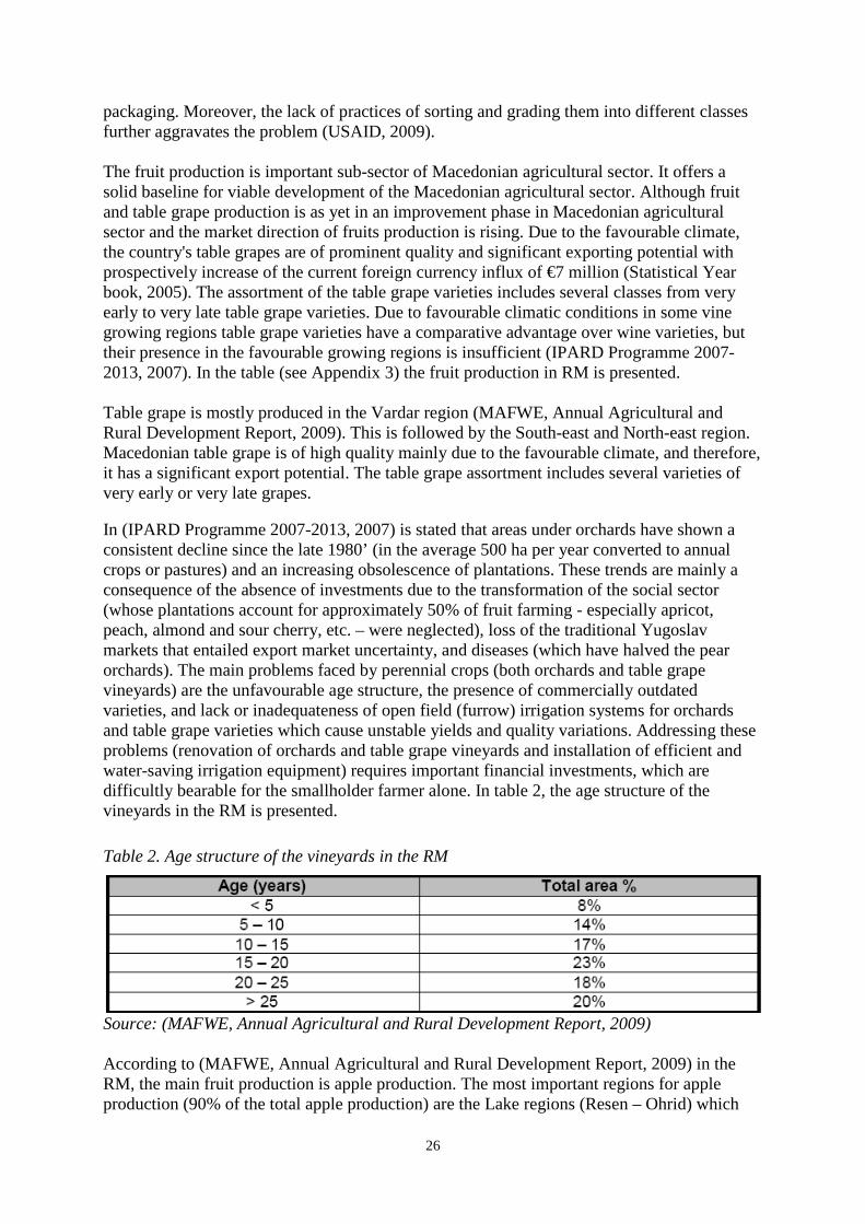
26

packaging. Moreover, the lack of practices of sorting and grading them into different classes further aggravates the problem (USAID, 2009). The fruit production is important sub-sector of Macedonian agricultural sector. It offers a solid baseline for viable development of the Macedonian agricultural sector. Although fruit and table grape production is as yet in an improvement phase in Macedonian agricultural sector and the market direction of fruits production is rising. Due to the favourable climate, the country's table grapes are of prominent quality and significant exporting potential with prospectively increase of the current foreign currency influx of €7 million (Statistical Year book, 2005). The assortment of the table grape varieties includes several classes from very early to very late table grape varieties. Due to favourable climatic conditions in some vine growing regions table grape varieties have a comparative advantage over wine varieties, but their presence in the favourable growing regions is insufficient (IPARD Programme 2007-2013, 2007). In the table (see Appendix 3) the fruit production in RM is presented. Table grape is mostly produced in the Vardar region (MAFWE, Annual Agricultural and Rural Development Report, 2009). This is followed by the South-east and North-east region. Macedonian table grape is of high quality mainly due to the favourable climate, and therefore, it has a significant export potential. The table grape assortment includes several varieties of very early or very late grapes. In (IPARD Programme 2007-2013, 2007) is stated that areas under orchards have shown a consistent decline since the late 1980’ (in the average 500 ha per year converted to annual crops or pastures) and an increasing obsolescence of plantations. These trends are mainly a consequence of the absence of investments due to the transformation of the social sector (whose plantations account for approximately 50% of fruit farming - especially apricot, peach, almond and sour cherry, etc. – were neglected), loss of the traditional Yugoslav markets that entailed export market uncertainty, and diseases (which have halved the pear orchards). The main problems faced by perennial crops (both orchards and table grape vineyards) are the unfavourable age structure, the presence of commercially outdated varieties, and lack or inadequateness of open field (furrow) irrigation systems for orchards and table grape varieties which cause unstable yields and quality variations. Addressing these problems (renovation of orchards and table grape vineyards and installation of efficient and water-saving irrigation equipment) requires important financial investments, which are difficultly bearable for the smallholder farmer alone. In table 2, the age structure of the vineyards in the RM is presented.

Table 2. Age structure of the vineyards in the RM

Source: (MAFWE, Annual Agricultural and Rural Development Report, 2009) According to (MAFWE, Annual Agricultural and Rural Development Report, 2009) in the RM, the main fruit production is apple production. The most important regions for apple production (90% of the total apple production) are the Lake regions (Resen – Ohrid) which

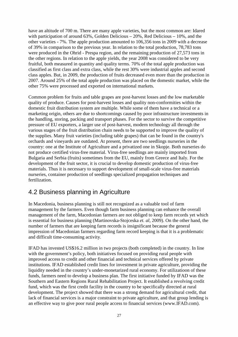
27

have an altitude of 700 m. There are many apple varieties, but the most common are: Idared with participation of around 63%, Golden Delicious – 20%, Red Delicious – 10%, and the other varieties - 7%. The apple production amounted to 106,356 tons in 2009 with a decrease of 39% in comparison to the previous year. In relation to the total production, 78,783 tons were produced in the Ohrid - Prespa region, and the remaining production of 27,573 tons in the other regions. In relation to the apple yields, the year 2008 was considered to be very fruitful, both measured in quantity and quality terms. 70% of the total apple production was classified as first class and extra class, while the rest 30% were industrial apples and second class apples. But, in 2009, the production of fruits decreased even more than the production in 2007. Around 25% of the total apple production was placed on the domestic market, while the other 75% were processed and exported on international markets. Common problem for fruits and table grapes are post-harvest losses and the low marketable quality of produce. Causes for post-harvest losses and quality non-conformities within the domestic fruit distribution system are multiple. While some of them have a technical or a marketing origin, others are due to shortcomings caused by poor infrastructure investments in the handling, storing, packing and transport phases. For the sector to survive the competitive pressure of EU exporters, a larger use of post-harvest, modern technology all through the various stages of the fruit distribution chain needs to be supported to improve the quality of the supplies. Many fruit varieties (including table grapes) that can be found in the country's orchards and vineyards are outdated. At present, there are two seedlings nurseries in the country: one at the Institute of Agriculture and a privatized one in Skopje. Both nurseries do not produce certified virus-free material. Virus-free seedlings are mainly imported from Bulgaria and Serbia (fruits) sometimes from the EU, mainly from Greece and Italy. For the development of the fruit sector, it is crucial to develop domestic production of virus-free materials. Thus it is necessary to support development of small-scale virus-free materials nurseries, container production of seedlings specialized propagation techniques and fertilization. 4.2 Business planning in Agriculture In Macedonia, business planning is still not recognized as a valuable tool of farm management by the farmers. Even though farm business planning can enhance the overall management of the farm, Macedonian farmers are not obliged to keep farm records yet which is essential for business planning (Martinovska-Stojceska et. al, 2009). On the other hand, the number of farmers that are keeping farm records is insignificant because the general impression of Macedonian farmers regarding farm record keeping is that it is a problematic and difficult time-consuming activity. IFAD has invested US$16.2 million in two projects (both completed) in the country. In line with the government’s policy, both initiatives focused on providing rural people with improved access to credit and other financial and technical services offered by private institutions. IFAD established credit lines for investment in private agriculture, providing the liquidity needed in the country’s under-monetarized rural economy. For utilizatioon of these funds, farmers need to develop a business plan. The first initiative funded by IFAD was the Southern and Eastern Regions Rural Rehabilitation Project. It established a revolving credit fund, which was the first credit facility in the country to be specifically directed at rural development. The project showed that there was a strong demand for agricultural credit, that lack of financial services is a major constraint to private agriculture, and that group lending is an effective way to give poor rural people access to financial services (www.IFAD.com).

28

Business planning on farm is important in terms of:

• Providing information about the farm performance • Improving the planning and the organization of the farm one year in advance • Better performance when an application for a loan is submitted

Nowadays, efforts are being made for familiarize the agricultural producers with the meaning, importance as well as the need for business planning on farm. For that purpose many workshops and trainings are organized. These types of training include explanation of the basic terms and definitions to the farmers, as well as the meaning of business planning and the reasons for become a practice. An important development is that all the eligible candidates (farms) that will use the EU supported funds will have to prepare a business plan. All these new developments have an impact on the farmers and are hopefully going to encourage the farmers to start with creating a farm business plan. The farmer as a manager could use the business plan as a valuable tool in the farm management and decision making process.

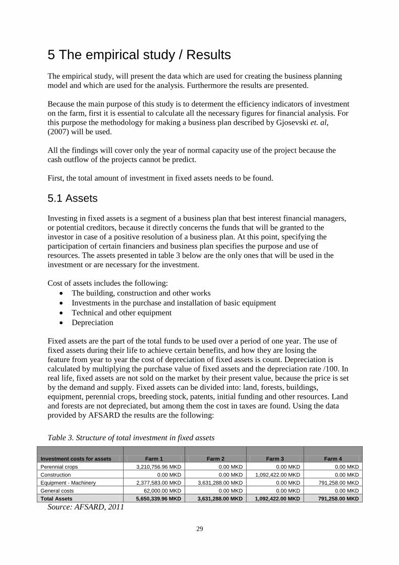
29

5 The empirical study / Results The empirical study, will present the data which are used for creating the business planning model and which are used for the analysis. Furthermore the results are presented. Because the main purpose of this study is to determent the efficiency indicators of investment on the farm, first it is essential to calculate all the necessary figures for financial analysis. For this purpose the methodology for making a business plan described by Gjosevski et. al, (2007) will be used. All the findings will cover only the year of normal capacity use of the project because the cash outflow of the projects cannot be predict. First, the total amount of investment in fixed assets needs to be found. 5.1 Assets Investing in fixed assets is a segment of a business plan that best interest financial managers, or potential creditors, because it directly concerns the funds that will be granted to the investor in case of a positive resolution of a business plan. At this point, specifying the participation of certain financiers and business plan specifies the purpose and use of resources. The assets presented in table 3 below are the only ones that will be used in the investment or are necessary for the investment. Cost of assets includes the following:

• The building, construction and other works • Investments in the purchase and installation of basic equipment • Technical and other equipment • Depreciation

Fixed assets are the part of the total funds to be used over a period of one year. The use of fixed assets during their life to achieve certain benefits, and how they are losing the feature from year to year the cost of depreciation of fixed assets is count. Depreciation is calculated by multiplying the purchase value of fixed assets and the depreciation rate /100. In real life, fixed assets are not sold on the market by their present value, because the price is set by the demand and supply. Fixed assets can be divided into: land, forests, buildings, equipment, perennial crops, breeding stock, patents, initial funding and other resources. Land and forests are not depreciated, but among them the cost in taxes are found. Using the data provided by AFSARD the results are the following:

Table 3. Structure of total investment in fixed assets

Investment costs for assets Farm 1 Farm 2 Farm 3 Farm 4 Perennial crops 3,210,756.96 MKD 0.00 MKD 0.00 MKD 0.00 MKD Construction 0.00 MKD 0.00 MKD 1,092,422.00 MKD 0.00 MKD Equipment - Machinery 2,377,583.00 MKD 3,631,288.00 MKD 0.00 MKD 791,258.00 MKD General costs 62,000.00 MKD 0.00 MKD 0.00 MKD 0.00 MKD Total Assets 5,650,339.96 MKD 3,631,288.00 MKD 1,092,422.00 MKD 791,258.00 MKD

Source: AFSARD, 2011

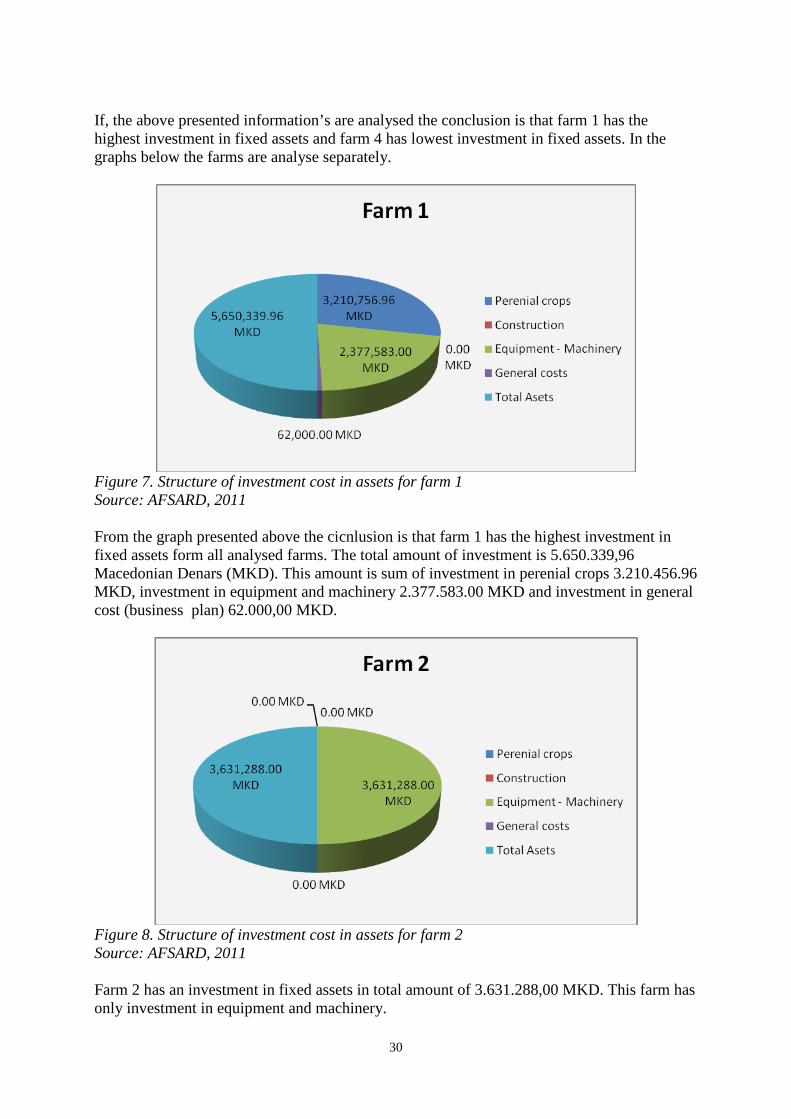
30

If, the above presented information’s are analysed the conclusion is that farm 1 has the highest investment in fixed assets and farm 4 has lowest investment in fixed assets. In the graphs below the farms are analyse separately.

Figure 7. Structure of investment cost in assets for farm 1 Source: AFSARD, 2011

From the graph presented above the cicnlusion is that farm 1 has the highest investment in fixed assets form all analysed farms. The total amount of investment is 5.650.339,96 Macedonian Denars (MKD). This amount is sum of investment in perenial crops 3.210.456.96 MKD, investment in equipment and machinery 2.377.583.00 MKD and investment in general cost (business plan) 62.000,00 MKD.

Figure 8. Structure of investment cost in assets for farm 2 Source: AFSARD, 2011 Farm 2 has an investment in fixed assets in total amount of 3.631.288,00 MKD. This farm has only investment in equipment and machinery.

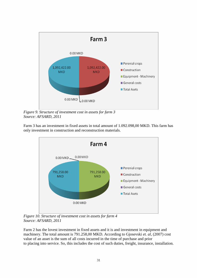
31

Figure 9. Structure of investment cost in assets for farm 3 Source: AFSARD, 2011 Farm 3 has an investment in fixed assets in total amount of 1.092.098,00 MKD. This farm has only investment in construction and reconstruction materials.

Figure 10. Structure of investment cost in assets for farm 4 Source: AFSARD, 2011 Farm 2 has the lovest investment in fixed assets and it is and investment in equipment and machinery. The total amount is 791.258,00 MKD. According to Gjosevski et. al, (2007) cost value of an asset is the sum of all costs incurred in the time of purchase and prior to placing into service. So, this includes the cost of such duties, freight, insurance, installation.

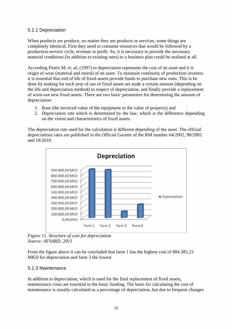
32

5.1.1 Depreciation When products are produce, no matter they are products or services, some things are completely identical. First they need to consume resources that would be followed by a production-service cycle, revenue or profit. So, it is necessary to provide the necessary material conditions (in addition to existing ones) to a business plan could be realised at all. According Florio M, et. al, (1997) to depreciation represents the cost of an asset and it is origin of wear (material and moral) of an asset. To maintain continuity of production investor, it is essential that end of life of fixed assets provide funds to purchase new ones. This is be done by making for each year of use of fixed assets set aside a certain amount (depending on the life and depreciation method) in respect of depreciation, and finally provide a replacement of worn-out new fixed assets. There are two basic parameters for determining the amount of depreciation:

1. Base (the invoiced value of the equipment or the value of property) and 2. Depreciation rate which is determined by the law, which is the difference depending

on the vision and characteristics of fixed assets.

The depreciation rate used for the calculation is different depending of the asset. The official depreciations rates are published in the Official Gazette of the RM number 64/2002, 98/2002 and 18/2010.

Figure 11. Structure of cost for depreciation Source: AFSARD, 2011 From the figure above it can be concluded that farm 1 has the highest cost of 884.385,23 MKD for depreciation and farm 3 the lowest. 5.1.3 Maintenance In addition to depreciation, which is used for the final replacement of fixed assets, maintenance costs are essential to the basic funding. The basis for calculating the cost of maintenance is usually calculated as a percentage of depreciation, but due to frequent changes

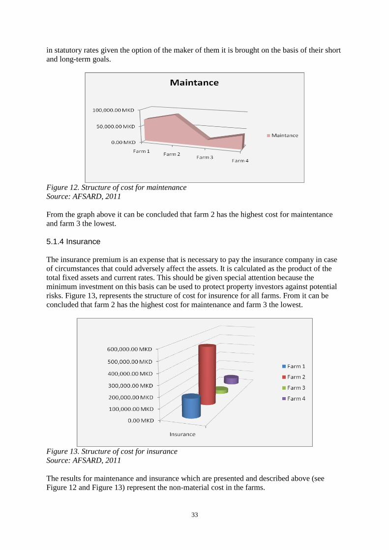
33

in statutory rates given the option of the maker of them it is brought on the basis of their short and long-term goals.

Figure 12. Structure of cost for maintenance Source: AFSARD, 2011 From the graph above it can be concluded that farm 2 has the highest cost for maintentance and farm 3 the lowest. 5.1.4 Insurance The insurance premium is an expense that is necessary to pay the insurance company in case of circumstances that could adversely affect the assets. It is calculated as the product of the total fixed assets and current rates. This should be given special attention because the minimum investment on this basis can be used to protect property investors against potential risks. Figure 13, represents the structure of cost for insurence for all farms. From it can be concluded that farm 2 has the highest cost for maintenance and farm 3 the lowest.

Figure 13. Structure of cost for insurance Source: AFSARD, 2011 The results for maintenance and insurance which are presented and described above (see Figure 12 and Figure 13) represent the non-material cost in the farms.

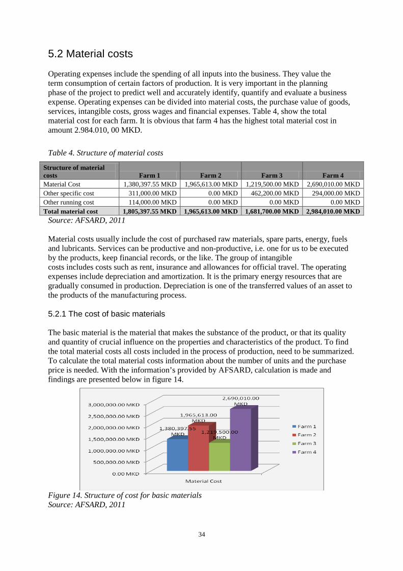
34

5.2 Material costs Operating expenses include the spending of all inputs into the business. They value the term consumption of certain factors of production. It is very important in the planning phase of the project to predict well and accurately identify, quantify and evaluate a business expense. Operating expenses can be divided into material costs, the purchase value of goods, services, intangible costs, gross wages and financial expenses. Table 4, show the total material cost for each farm. It is obvious that farm 4 has the highest total material cost in amount 2.984.010, 00 MKD.

Table 4. Structure of material costs

Structure of material costs Farm 1 Farm 2 Farm 3 Farm 4 Material Cost 1,380,397.55 MKD 1,965,613.00 MKD 1,219,500.00 MKD 2,690,010.00 MKD Other specific cost 311,000.00 MKD 0.00 MKD 462,200.00 MKD 294,000.00 MKD Other running cost 114,000.00 MKD 0.00 MKD 0.00 MKD 0.00 MKD Total material cost 1,805,397.55 MKD 1,965,613.00 MKD 1,681,700.00 MKD 2,984,010.00 MKD

Source: AFSARD, 2011 Material costs usually include the cost of purchased raw materials, spare parts, energy, fuels and lubricants. Services can be productive and non-productive, i.e. one for us to be executed by the products, keep financial records, or the like. The group of intangible costs includes costs such as rent, insurance and allowances for official travel. The operating expenses include depreciation and amortization. It is the primary energy resources that are gradually consumed in production. Depreciation is one of the transferred values of an asset to the products of the manufacturing process. 5.2.1 The cost of basic materials The basic material is the material that makes the substance of the product, or that its quality and quantity of crucial influence on the properties and characteristics of the product. To find the total material costs all costs included in the process of production, need to be summarized. To calculate the total material costs information about the number of units and the purchase price is needed. With the information’s provided by AFSARD, calculation is made and findings are presented below in figure 14.

Figure 14. Structure of cost for basic materials Source: AFSARD, 2011

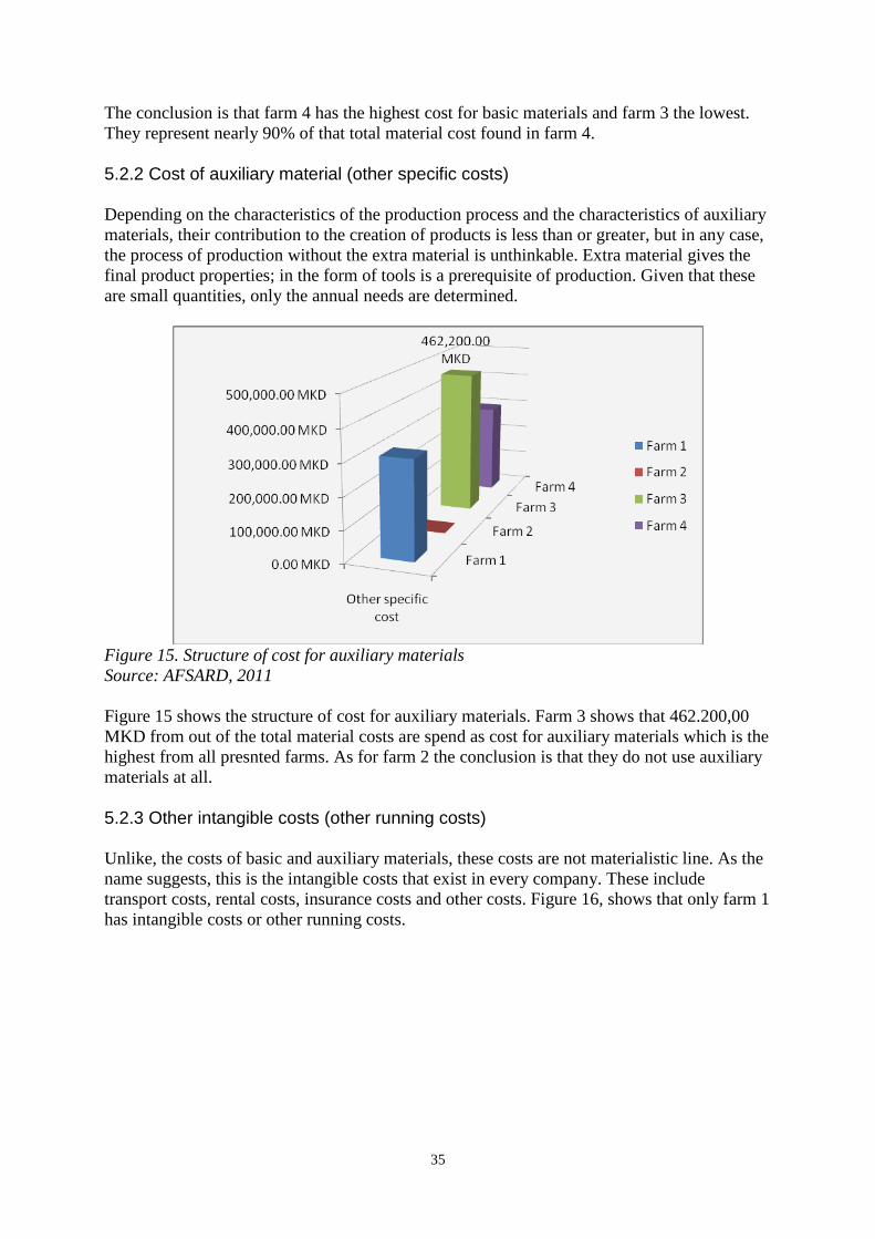
35

The conclusion is that farm 4 has the highest cost for basic materials and farm 3 the lowest. They represent nearly 90% of that total material cost found in farm 4.

5.2.2 Cost of auxiliary material (other specific costs) Depending on the characteristics of the production process and the characteristics of auxiliary materials, their contribution to the creation of products is less than or greater, but in any case, the process of production without the extra material is unthinkable. Extra material gives the final product properties; in the form of tools is a prerequisite of production. Given that these are small quantities, only the annual needs are determined.

Figure 15. Structure of cost for auxiliary materials Source: AFSARD, 2011

Figure 15 shows the structure of cost for auxiliary materials. Farm 3 shows that 462.200,00 MKD from out of the total material costs are spend as cost for auxiliary materials which is the highest from all presnted farms. As for farm 2 the conclusion is that they do not use auxiliary materials at all. 5.2.3 Other intangible costs (other running costs) Unlike, the costs of basic and auxiliary materials, these costs are not materialistic line. As the name suggests, this is the intangible costs that exist in every company. These include transport costs, rental costs, insurance costs and other costs. Figure 16, shows that only farm 1 has intangible costs or other running costs.

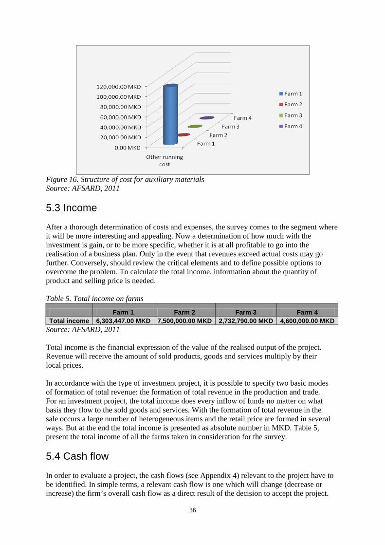
36

Figure 16. Structure of cost for auxiliary materials Source: AFSARD, 2011 5.3 Income After a thorough determination of costs and expenses, the survey comes to the segment where it will be more interesting and appealing. Now a determination of how much with the investment is gain, or to be more specific, whether it is at all profitable to go into the realisation of a business plan. Only in the event that revenues exceed actual costs may go further. Conversely, should review the critical elements and to define possible options to overcome the problem. To calculate the total income, information about the quantity of product and selling price is needed. Table 5. Total income on farms

Farm 1 Farm 2 Farm 3 Farm 4 Total income 6,303,447.00 MKD 7,500,000.00 MKD 2,732,790.00 MKD 4,600,000.00 MKD

Source: AFSARD, 2011

Total income is the financial expression of the value of the realised output of the project. Revenue will receive the amount of sold products, goods and services multiply by their local prices. In accordance with the type of investment project, it is possible to specify two basic modes of formation of total revenue: the formation of total revenue in the production and trade. For an investment project, the total income does every inflow of funds no matter on what basis they flow to the sold goods and services. With the formation of total revenue in the sale occurs a large number of heterogeneous items and the retail price are formed in several ways. But at the end the total income is presented as absolute number in MKD. Table 5, present the total income of all the farms taken in consideration for the survey. 5.4 Cash flow In order to evaluate a project, the cash flows (see Appendix 4) relevant to the project have to be identified. In simple terms, a relevant cash flow is one which will change (decrease or increase) the firm’s overall cash flow as a direct result of the decision to accept the project.

37

Relevant cash flows thus, deal with changes or increments to the firm’s existing cash flows. These flows are also known as incremental or marginal cash flows (Dayananda, 2002). In the tables (see Appendix 4) a cash flows of all farms taken in consideration for the survey are presented. All the data presented (see Appendix 4) will be used further for calculation for the financial ratios. 5.5 Income statement Income statement (see Appendix 5) shows the total revenues and expenses during a time. An income statement is sometimes called a “profit and loss statement,” an “operating statement,” or a “statement of operations.” Essentially, it tells whether or not the firm is making money. In the tables (see Appendix 5) an income statements of all farms taken in consideration for the survey are presented. 5.6 Balance sheet The purpose of a balance sheet is to (see Appendix 6) list all the assets of a business and all of its financial resources at a given point in time. “By definition, a company’s assets and resources must be exactly equal. This is the fundamental principle of double-entry accounting. When an item is purchased, it is either capitalized or expensed. If it is capitalized, it will appear on the asset side of the balance sheet, and if expensed, it will lead to a reduction in earnings and thus shareholders’ equity. The double-entry for this purchase is either a reduction in cash (i.e. a decrease in an asset) or a commitment (i.e. a liability) to the vendor (i.e. an increase in a liability). According to the algebra of accounting, assets and resources (equity and liabilities) always carry the opposite sign, so the equilibrium of the balance sheet is always maintained” Vernimmen et. al (2009). In the tables (see Appendix 6) balance sheets of all farms taken in consideration for the survey are presented. 5.7 Financial ratios As it is explained above dynamical ratios are usually expressed as a percent or as times per period. A ratio can be computed from any pair of numbers. Given the large quantity of variables included in financial statements, a very long list of meaningful ratios can be derived. A standard list of ratios or standard computation of them does not exist. Each author and source on financial analysis uses a different list (Higgins. C, 2000) .This survey presents frequently utilised and discussed ratios (see Appendix 7). In the tables (see Appendix 7) the most used financial ratios of all farms taken in consideration for the survey are presented. 5.8 NPV, IRR and Payback indicators According to Higgins C. R, (2000) an investment’s NPV is the present value of all incremental cash flows associated with the investment. This includes the initial cash outflow

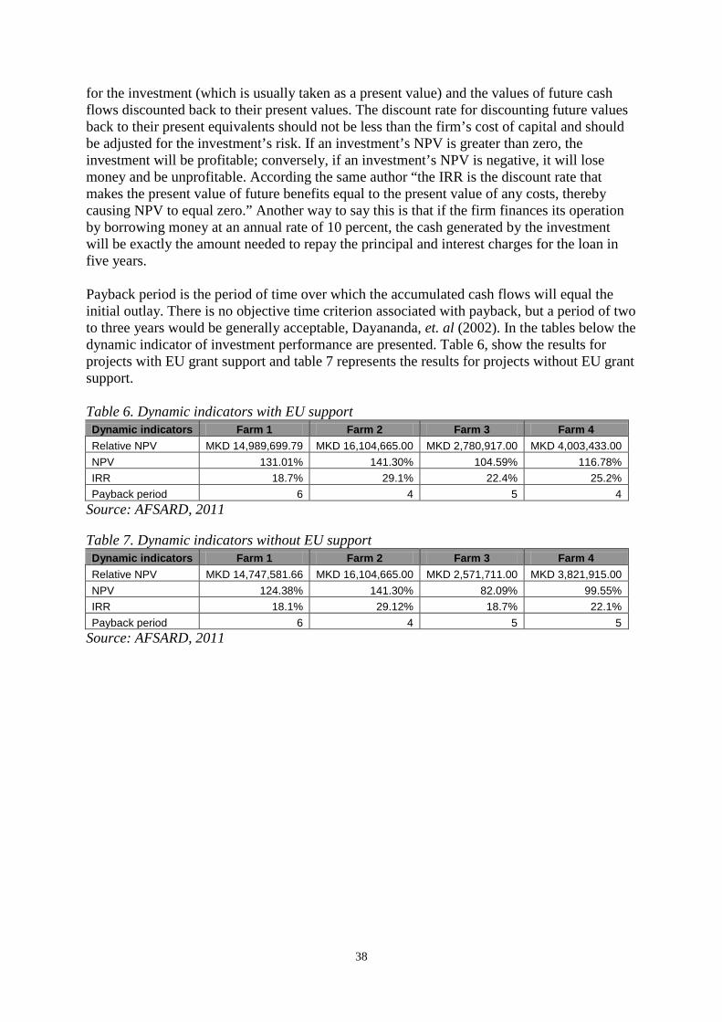
38

for the investment (which is usually taken as a present value) and the values of future cash flows discounted back to their present values. The discount rate for discounting future values back to their present equivalents should not be less than the firm’s cost of capital and should be adjusted for the investment’s risk. If an investment’s NPV is greater than zero, the investment will be profitable; conversely, if an investment’s NPV is negative, it will lose money and be unprofitable. According the same author “the IRR is the discount rate that makes the present value of future benefits equal to the present value of any costs, thereby causing NPV to equal zero.” Another way to say this is that if the firm finances its operation by borrowing money at an annual rate of 10 percent, the cash generated by the investment will be exactly the amount needed to repay the principal and interest charges for the loan in five years. Payback period is the period of time over which the accumulated cash flows will equal the initial outlay. There is no objective time criterion associated with payback, but a period of two to three years would be generally acceptable, Dayananda, et. al (2002). In the tables below the dynamic indicator of investment performance are presented. Table 6, show the results for projects with EU grant support and table 7 represents the results for projects without EU grant support. Table 6. Dynamic indicators with EU support Dynamic indicators Farm 1 Farm 2 Farm 3 Farm 4 Relative NPV MKD 14,989,699.79 MKD 16,104,665.00 MKD 2,780,917.00 MKD 4,003,433.00 NPV 131.01% 141.30% 104.59% 116.78% IRR 18.7% 29.1% 22.4% 25.2% Payback period 6 4 5 4

Source: AFSARD, 2011 Table 7. Dynamic indicators without EU support Dynamic indicators Farm 1 Farm 2 Farm 3 Farm 4 Relative NPV MKD 14,747,581.66 MKD 16,104,665.00 MKD 2,571,711.00 MKD 3,821,915.00 NPV 124.38% 141.30% 82.09% 99.55% IRR 18.1% 29.12% 18.7% 22.1% Payback period 6 4 5 5

Source: AFSARD, 2011

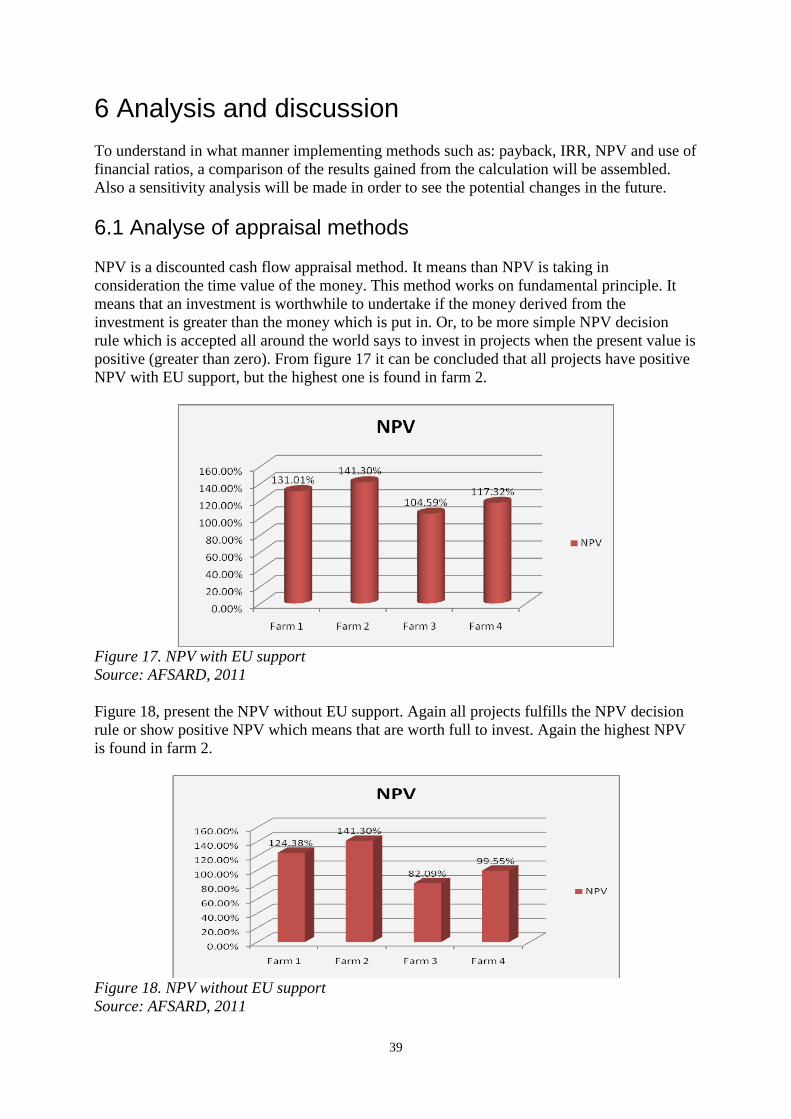
39

6 Analysis and discussion To understand in what manner implementing methods such as: payback, IRR, NPV and use of financial ratios, a comparison of the results gained from the calculation will be assembled. Also a sensitivity analysis will be made in order to see the potential changes in the future. 6.1 Analyse of appraisal methods

NPV is a discounted cash flow appraisal method. It means than NPV is taking in consideration the time value of the money. This method works on fundamental principle. It means that an investment is worthwhile to undertake if the money derived from the investment is greater than the money which is put in. Or, to be more simple NPV decision rule which is accepted all around the world says to invest in projects when the present value is positive (greater than zero). From figure 17 it can be concluded that all projects have positive NPV with EU support, but the highest one is found in farm 2.

Figure 17. NPV with EU support Source: AFSARD, 2011 Figure 18, present the NPV without EU support. Again all projects fulfills the NPV decision rule or show positive NPV which means that are worth full to invest. Again the highest NPV is found in farm 2.

Figure 18. NPV without EU support Source: AFSARD, 2011

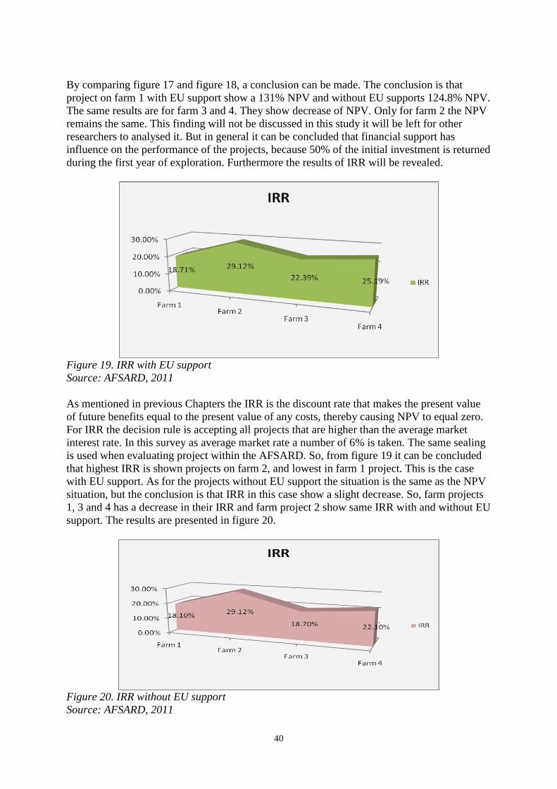
40

By comparing figure 17 and figure 18, a conclusion can be made. The conclusion is that project on farm 1 with EU support show a 131% NPV and without EU supports 124.8% NPV. The same results are for farm 3 and 4. They show decrease of NPV. Only for farm 2 the NPV remains the same. This finding will not be discussed in this study it will be left for other researchers to analysed it. But in general it can be concluded that financial support has influence on the performance of the projects, because 50% of the initial investment is returned during the first year of exploration. Furthermore the results of IRR will be revealed.

Figure 19. IRR with EU support Source: AFSARD, 2011

As mentioned in previous Chapters the IRR is the discount rate that makes the present value of future benefits equal to the present value of any costs, thereby causing NPV to equal zero. For IRR the decision rule is accepting all projects that are higher than the average market interest rate. In this survey as average market rate a number of 6% is taken. The same sealing is used when evaluating project within the AFSARD. So, from figure 19 it can be concluded that highest IRR is shown projects on farm 2, and lowest in farm 1 project. This is the case with EU support. As for the projects without EU support the situation is the same as the NPV situation, but the conclusion is that IRR in this case show a slight decrease. So, farm projects 1, 3 and 4 has a decrease in their IRR and farm project 2 show same IRR with and without EU support. The results are presented in figure 20.

Figure 20. IRR without EU support Source: AFSARD, 2011

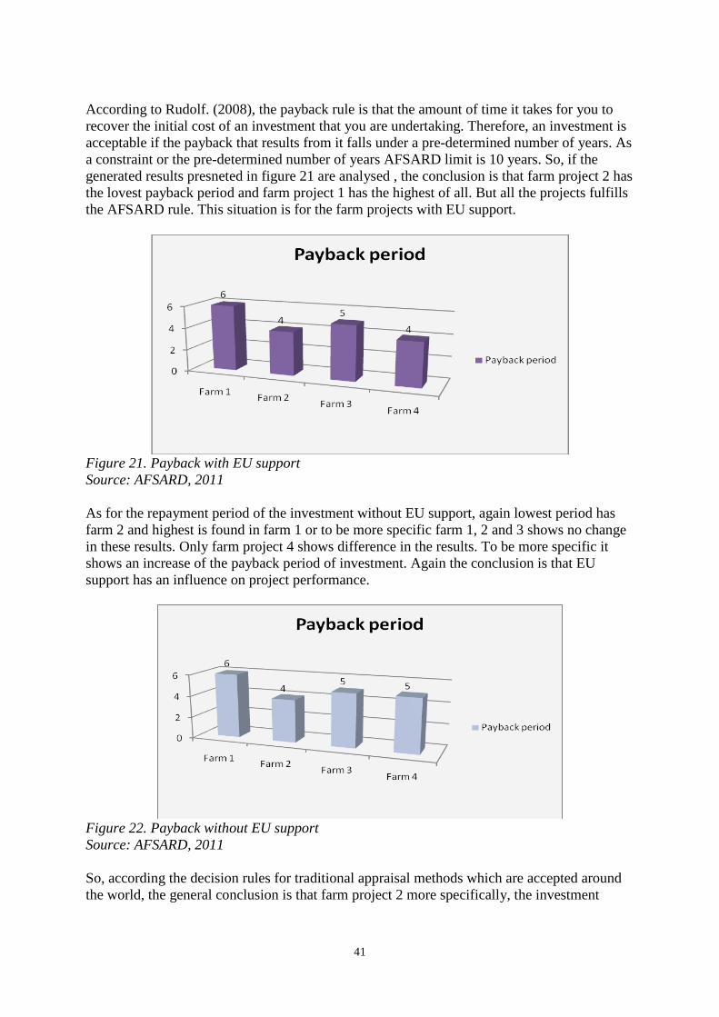
41

According to Rudolf. (2008), the payback rule is that the amount of time it takes for you to recover the initial cost of an investment that you are undertaking. Therefore, an investment is acceptable if the payback that results from it falls under a pre-determined number of years. As a constraint or the pre-determined number of years AFSARD limit is 10 years. So, if the generated results presneted in figure 21 are analysed , the conclusion is that farm project 2 has the lovest payback period and farm project 1 has the highest of all. But all the projects fulfills the AFSARD rule. This situation is for the farm projects with EU support.

Figure 21. Payback with EU support Source: AFSARD, 2011

As for the repayment period of the investment without EU support, again lowest period has farm 2 and highest is found in farm 1 or to be more specific farm 1, 2 and 3 shows no change in these results. Only farm project 4 shows difference in the results. To be more specific it shows an increase of the payback period of investment. Again the conclusion is that EU support has an influence on project performance.

Figure 22. Payback without EU support Source: AFSARD, 2011

So, according the decision rules for traditional appraisal methods which are accepted around the world, the general conclusion is that farm project 2 more specifically, the investment

42

indicates the best efficiency indicators of all analysed investments and that even with or without EU support these projects are good to invest. But, with this methods and rules still the managares/farmers are not certain what outcomes will generate, if investing in it. It is quite clear that investment decision making never takes location under circumstances of sureness, but only beneath those of doubt or risk. It is therefore necessary to define and find the investment decision- making dilemma in its real situation, and probably and proper and correct solutions. Due to cause of distinct components it is potentially likely that desired values are not recognized in the future. If the managares/farmers want to take into concern all likely penalties, they have to examine, in advance, the results of possible changes of the initial values on the results generated by the computation. Solutions of problems, linked with investment under circumstances of sureness, especially assessment of investment projects in circumstances of sureness and risk, are probable to execute applying different methods and techniques. According to Jovanovic, (1999), the best known methods employed in investment decision making are: “break-even analysis, sensitivity analysis, scenario method, theory of games and decision making theory, etc.” The main goal of sensitivity analysis is to gain insight into which assumptions are critical, i.e. which assumptions affect choice. The process involves various ways of changing input values of the model to see the effect on the output value. In some decision situations you can use a single model to investigate several alternatives. In other cases, you may use a separate spreadsheet model for each alternative. Dayananda, et. al (2002), introduces two mechanical methods for analysing projects under risk. The first method is known as sensitivity analysis and the second method is known as break-even analysis. In this study only the first method will be revealed, or to be more specific only the sensitivity analysis method will be used and only for the NPV method, due to the time constraints. With applying the method of sensitivity analysis, it is likely to find the highest or lowest points which one value may get while, but, still allowing an investment project to be reasonable and suitable for implementation. As the basis for evaluation the outputs and the inputs of an investment will be taken in consideration. A model which will be used and it is developed by Jovanovic, (1999) have a mathematical expression:

NI=P-T-I

where the symbols stand for: P- projects incomes T - project costs I - value of investments In order to see and analyse all of these possible situations in the future during the investment decision making, an variations of the input parameters for calculation of NPV, IRR and payback period by attributing the relating corrective coefficients is needed, The mathematical expression is:

NI= d*P- n*T- k*I

where the symbols stand for: d - income correction factor m - cost correction factor

43

k - the investment value correction factor In this study, only the simultaneous effects of discount rate and the total value of investment on the NPV criterion is analysed. This means that only the factors “p” and “k”, vary, while factors “d” and “m” remain constant. The findings by using this method was that when holding all the criterion factors constant and change only the investment value correction factor, the NPV results are low and they become lower how the investment value correction factor is increased. Also, by holding all the criterion factors constant and change only the discount rate correction factor, the result is that again the lowest NPV for all projects is generated. In the tables (see Appendix 8-11) the sensitivity analysis of NPV for each farm taken in consideration for the survey is presented. The table (see Appendix 8) shows the results generated by using the method described by Jovanovic, (1999). The conclusion is that for discount rate of p=10%, farm 1 allows a transgression of the investment value limit of 22, 9%. For the same value of the discount rate a transgression of the investment value limit of 25, 4% gives a negative and unacceptable value of the NPV. With this method the business owner can see the potential changes in the future and bring decisions easily. The table (see Appendix 9), show the results for farm 2, generated by using the method described by Jovanovic, (1999) It can be concluded that farm 2 for discount rate of p=30%, allows a transgression of the investment value limit of 22,9%. For the same value of the discount rate a transgression of the investment value limit of 25, 4% gives a negative and unacceptable result of the NPV. For a discount rate p=22% a transgression of the investment value limit of 30,0% is allowed. From the table (see Appendix 10), can be concluded that farm 3 for discount rate p=18% allows a transgression of the investment value limit of 22,9%. For the same value of the discount rate transgression of the investment value limit of 25, 4% gives a negative and unacceptable result of the NPV. For a discount rate p=12% a transgression of the investment value limit of 30, 0% is allowed. This is acceptable for the business owners if they take in consideration the NPV rule. When farm 4 was analysed, the most interesting results were found (see Appendix 11). The results show that for discount rate p=18% a transgression of the investment value limit of 30,0% is allowed. For a discount rate p=30% a transgression of the investment value limit of 30, 0% is allowed which is acceptable when taking in consideration the NPV rule. Hence, it seems that this investment can stand more increase of correction factors. 6.2 Analyse of financial ratios Furthermore, analyse of financial ratios will be performed. The results are presented in Appendix 7. Financial analysis is one of the many tools useful in valuation because it helps the financial analyst gauge returns and risks. According to Fabozzi & Peterson, (2003) a financial ratio is a comparison between one bit of financial information and another. Consider the ratio of current assets to current liabilities, better known as the current ratio. This ratio is a comparison between assets that can be readily turned into cash (current assets) and the

44

obligations that are due in the near future (current liabilities). A current ratio of 2 or 2:1 means that the business owner have twice as much in current assets as it is need to satisfy the obligations due in the near future. Starting with the liquidity measures first the net working capital ratio will be analyse. Net working capital is a measurement of the operating liquidity available for a company to use in developing and growing it is business. This is relying largely on the amount of debt owed by the company. It should not come as a surprise that having plenty of working capital tends to help companies achieve more success. This follows because working capital allows companies to grow smoothly and make necessary improvements to their corporate operations. On the other hand, companies that are operating with negative working capital may not have the financial support or flexibility to grow or improve, even when such developments would be indicated. Hence, working capital can be an indicator of the overall strength of a company. So, using the results calculated by using data provided by AFSARD it can be concluded that all farms have positive net working capital, Farm 1 indicates the highest of all, with an amount of 3.752.717,72 MKD. General conclusion is that the more net working capital a business has, the less risky it is, as it has the ability to cover current liabilities as they come due. Second liquidity measure which is essential for guiding the financial health of a company is the ratio of net working capital to sales. It measures how well the company's cash is being used to generate sales. A high ratio of net working capital to sales is usually a positive sign, indicating the company is more able to use its working capital to generate sales. Although, measuring the performance of a company for just one period reveals how well it is using its cash for that single period. This ratio is much more effectively used over a number of periods. This ratio can help uncover questionable management decisions such as relaxing credit requirements to potential customers to increase sales, increasing inventory levels to reduce order fulfillment cycle times and slowing payment to vendors and suppliers in an effort to hold on to its cash. By analysing the results provided in the financial statements, a net working capital was calculated for each farm. Again highest amount of net working capital has farm 1, with an amount of 60%. Compare with the other farms, it says that this farm use most efficient the working capital to generate sales. Worst situation is found in farm 4. Next, the results for ratio of net working capital to current assets will be analysed. As mentioned above according to Pike & Neale, (2006) this ratio “expresses the percentage by which a firm’s current assets can shrink before becoming less than the amount needed to cover current liabilities.” A high ratio is usually a positive sign and low ratio indicates the company may have too many total current liabilities. Analysing the tables (see Appendix 7) it can be concluded that for this ratio farm 3 indicates the best performance with an amount of 47%. Worst case is for farm 4 with an amount of 9%. The current ratio is a more dependable indication of liquidity than the net working capital. It indicates the firm’s ability to meet or cover its current liabilities using its current assets. There are no set criteria for the normal current ratio, as that is dependent on the business itself. If the business has predictable cash flow, it can operate with a lower current ratio. The ratio of 2.0 is considered acceptable for most businesses. A ratio of 2.0 would allow a company to lose 50% of its current assets and still be able to cover current liabilities. For most businesses, this is an adequate margin of safety. The results presented in the tables (see Appendix 7), reviled that farm 3 has the highest current ratio, contrary to farm 2 and farm 4 who has the lowest ratio.

45

The current ratio of 1.9 indicates that farm 3 has approximately two times as much as it needs to cover its current obligations during the year. An alternative to the current ratio is the quick ratio, also called the acid-test ratio, which use a slightly different set of current accounts to cover the same current liabilities as in the current ratio. In the quick ratio, the least liquid of the current asset accounts, inventory, is excluded. A quick ratio of one or greater is usually recommended. Less than one suggests that the company cannot meet its everyday liabilities without resorting to bank borrowings, but that is dependent on the business itself. These ratios can be use to see if the business is in any risk of insolvency. It is also able to assess the ability to increase or decrease current assets for business strategy. The creditors will use these ratios to determine whether to extend credit or not. From the results it can be concluded that all farms meet these expectations or have quick ratio greater than 1. The highest, can be found in farm 3 and lowest in farm 2 and farm 4. Ratios that are typically used to analyse how well a company uses its assets and liabilities, internally are the efficiency ratios. They can calculate the turnover of receivables, the repayment of liabilities, the quantity and usage of equity and the general use of inventory and machinery. These ratios are meaningful when compared to peers in the same industry and can identify businesses that are better managed relative to the others. Also, efficiency ratios are important because an improvement in the ratios usually translate to improved profitability. A higher fixed-asset turnover ratio shows that the company has been more effective in using the investment in fixed assets to generate revenues or to be more specific higher the ratio, greater is the intensive utilisation of fixed assets. Lower ratio means under-utilisation of fixed assets. Highest ratio of all farms that were analysed is found in farm 4 with an amount of 2.1 and lowest is found in farm 2 with an amount of 0,59. The total asset turnover ratio measures the ability of a company to use its assets to generate sales. The total asset turnover ratio considers all assets including fixed assets, such as plant and equipment, as well as inventory and accounts receivable. The lower the total asset turnover ratio is, the more worsen the firm's sales. This may indicate a problem with one or more of the asset categories composing total assets (inventory, receivables, or fixed assets). Issues that can lower the total asset turnover ratio could be a problem with inventory, with accounts receivable and with fixed assets. Regarding the inventory the firm could be holding obsolete inventory and not selling inventory fast enough. With regard to accounts receivable, the firm's collection period could be too long and credit accounts may be on the books too long. Fixed assets, such as plant and equipment, could be sitting idle instead of being used to their full capacity. Back to our farms a highest total assets turnover ratio can be found in farm 4. Farm 3 show lower result, with an amount of 0,6 and worst result is found in farm 2. A leverage ratio is any ratio used to calculate the financial leverage of a company, used to get an idea of the company's methods of financing or to measure its ability to meet financial obligations. In this study, only total debt to equity ratio will be analysed. It measures how much money a company should safely be able to borrow over long periods of time. The normal level of debt to equity has changed over time and is different between countries, and depends on both economic factors and society's general feeling towards credit. A high total debt to equity ratio generally means that a company has been aggressive in financing its growth with debt. This can result in volatile earnings as a result of the additional interest expense. If a lot of debt is used to finance increased operations (high debt to equity), the company could potentially generate more earnings than it would have without this outside financing. Analysing the results from the tables (see Appendix 7), it is obvious that farm 4 has

46

highest ratio with an amount of 2.62. The lowest ratio was found in farm 3. As mentioned before a high ratio is not a favourable one which means that farm 3 show best results. Profitability ratios are class of financial metrics that are used to assess a business's ability to generate earnings, as compared to its expenses and other relevant costs incurred for a specific period of time. For most of these ratios, having a higher value relative to a competitor's ratio or the same ratio from a previous period is indicative that the company is doing well. Profit margin ratios compare components of income with sales. They give the business owner an idea of which factors make up a firm’s income and are usually expressed as a portion of each dollar of sales. The gross profit margin indicates the percentage of each sales dollar remaining after a business has paid for its goods. The highest the gross profit margin, the better. In this study farm 3 have highest gross profit margin with an amount of 62% and lowest is found in farm 2 with an amount of 20%. Operating profit margin represents the pure operations profits, ignoring interest and taxes. A high operating profit margin is preferred. The operating profit margin looks at EBIT as a percentage of sales. The operating profit margin ratio is a measure of overall operating efficiency, incorporating all of the expenses of ordinary, daily business activity. It shows how much cash is thrown off after most of the expenses are met. A high operating profit margin means that the company has good cost control and that sales are increasing faster than costs, which is the optimal situation for the company. Farm 2 shows highest percentage, 56% of this ratio and farm 4 lowest of all with an amount of 19%. The net profit margin tells us the net income generated from each MKD of sales. It considers financing costs that the operating profit margin does not take in consideration. Net profit margin is the number of MKD of after-tax profit a firm generates per MKD of sales. If a firm generates 1.00 MKD of sales revenue, for example and has a 5 percent net profit margin, that means it generates 5,00 MKD of profit. In this survey, highest percentage is shown by farm 3 and 2 with an amount of 50% and lowest one is shown by farm 4 with an amount of 7%. Hence, it means that farm 3 and 2 generate 50,00 MKD of profit and farm 4 only 7,00 MKD. The last financial ratio which is analysed is the ratio of ROA. Return on assets allows the business owner to calculate how efficiently the company is using their total asset to generate sales. Total assets include all current assets such as cash, inventory, and accounts receivable in addition to fixed assets such as plant and equipment. The ROA figure gives investors and business owners an idea of how effectively the company is converting the money it has to invest into net income. The higher the ROA number is, the better, because the company is earning more money on less investment. Again the best performance is found in farm 3 with an amount of 18% and lowest one is found in farm 2 with an amount of 5%. Some of the above mentioned ratios which were analysed and compared between them self (for the farms used for this survey) are presented in figure 23. Furthermore, these ratios will be used to calculate the average ratios and used for a comparasion with the average ratios for the EU countries.

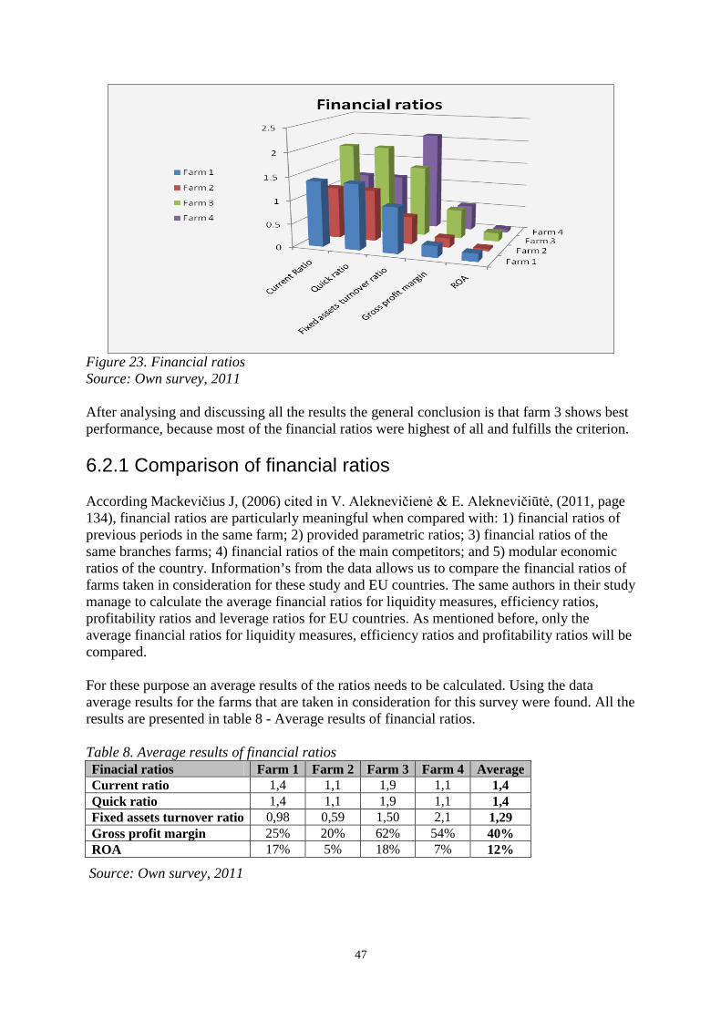
47

Figure 23. Financial ratios Source: Own survey, 2011 After analysing and discussing all the results the general conclusion is that farm 3 shows best performance, because most of the financial ratios were highest of all and fulfills the criterion. 6.2.1 Comparison of financial ratios According Mackevičius J, (2006) cited in V. Aleknevičienė & E. Aleknevičiūtė, (2011, page 134), financial ratios are particularly meaningful when compared with: 1) financial ratios of previous periods in the same farm; 2) provided parametric ratios; 3) financial ratios of the same branches farms; 4) financial ratios of the main competitors; and 5) modular economic ratios of the country. Information’s from the data allows us to compare the financial ratios of farms taken in consideration for these study and EU countries. The same authors in their study manage to calculate the average financial ratios for liquidity measures, efficiency ratios, profitability ratios and leverage ratios for EU countries. As mentioned before, only the average financial ratios for liquidity measures, efficiency ratios and profitability ratios will be compared. For these purpose an average results of the ratios needs to be calculated. Using the data average results for the farms that are taken in consideration for this survey were found. All the results are presented in table 8 - Average results of financial ratios. Table 8. Average results of financial ratios Finacial ratios Farm 1 Farm 2 Farm 3 Farm 4 Average Current ratio 1,4 1,1 1,9 1,1 1,4 Quick ratio 1,4 1,1 1,9 1,1 1,4 Fixed assets turnover ratio 0,98 0,59 1,50 2,1 1,29 Gross profit margin 25% 20% 62% 54% 40% ROA 17% 5% 18% 7% 12%

Source: Own survey, 2011

48

It was found out that the average current ratio for the farms used for this survey is 1.4, that average quick ratio is also 1.4. Further more, it was found out that the average total assets turnover ratio is 0.49, the average gross profit margin is 40% and the average ROA is 12%. In their study in V. Aleknevičienė & E. Aleknevičiūtė, (2011) calculated that average current ratio in EU country farms is 4.5. The highest current ratio was found in Spain with 115.7 and lowest in UK with 2.1. All the results are presented in the figure - Current ratios in the EU countries’ farms (see Appendix 12). So, by comparing the average current ratio of Macedonian farms which is 1.4 with the average current ratio of EU countries farms which is 4.5, it can be concluded that Macedonian farms are below the average current ratio of EU countries‟ farms and need to work harder if they want to more competitive on the world market. The same authors V. Aleknevičienė & E. Aleknevičiūtė, (2011), in their study found out that the average quick ratio in the EU countries’ farms is 3.1, average ROA in the EU farms is 6.2%. Compare with Macedonian farms it can be concluded that they have average quick ratio below the EU countries’ farms. As for the average ROA it can be concluded that for Macedonian farms, this ratio is higher that the EU countries’ farms. As mentioned above the return on assets allows the business owner to calculate how efficiently the company is using their total asset base to generate sales. It gives investors an idea of how effectively the company is converting the money it has to invest into net income. So, results show that Macedonian farms use their total asset to generate sales more effectively that EU country’ farms. In the same study V. Aleknevičienė & E. Aleknevičiūtė, (2011), showed that the average gross profit margin in the EU countries’ farms is 78.2 % and gross profit margin varied from 94.7% in Slovenia‘s farms to 41.9% in Slovakia‘s farms. Excluding Slovenia‘s and Slovakia‘s farms, the highest gross production profit margins were found in Austria (92.9%) and Poland (90.6%), while the lowest margins were in the Czech Republic (45.3%). Compare with the average gross profit margin in Macedonia farms which is 40%, it can be conclude that again the Macedonian farms are below the average. Furthermore V. Aleknevičienė & E. Aleknevičiūtė, (2011), stated that the average fixed assets turnover ratio in the EU countries’ farms is EUR 0.14. The same authors stated that within the EU countries’ farms this ratio varied from EUR 0.29 in Bulgaria to EUR 0.04 in Ireland. Compare to the results for Macedonian farms presented in this survey, it can be concluded that they earn 1, 29 MKD gross farm income for 1 MKD of assets, or converted in EUR is 0.02 which is less then EU countries’ farms. This indicates that Macedonian farms are less effective by using the investment in fixed assets in order to generate revenues. All the compared results are presented in figure (see Appendix 13).

49

7 Conclusions This Chapter gives to answer of the main objectives and study questions defined in the introductory part. As mentioned earlier the prime aim of this study is to create a model which will create a new income opportunities for farmers and promote sustainable agriculture practices and get the most realistic indicators of economic effectiveness which will help the farmers independently evaluate the economic effects of the investments on their business. The objective of this study is to understand a business planning model in order to facilitate the farmer’s decision making process, analyse the impacts of potential changes in future, identify the three key financial statements and use financial ratios to guide their financial health. The development of the areas of agriculture, regions and human resources is supported by EU assistance for the first time, apart from capacity building projects. Public awareness is at the moment being addressed by campaigns organized through the all relevant institutions and the main emphasis is placed on the availability of the funds. The eligible persons more specificly the farmers, have to primarily be aware that the funds are available to them as well, as opposed to the financing until now, which was available for the state institutions only. They need to know that IPARD is brought closer to the citizens, especially groups like the small farmers who need trainings. Previously, it was indicated that the sorts of optimizing models used by economists serve the purpose of providing guidance for choices. Indeed one of the important roles of economic model is to keep track of benefits and costs. The idea of business planning is a fundamental one in economics, and would be very difficult to use without a theoretical model of economic linkages. This brings up the important point that the correct way to measure an economic benefit or cost can only be determined in light of a model: a specification of what objectives and the constraints facing an economic agent. That is why it was an essential to create a model which provides the farmers with information’s sufficient for decision making. The findings presented in the previous Chapters show that by using the appraisal methods such as NPV, IRR, payback and sensitivity analysis method, the farmers can bring easily decisions such as invest in their business or just simply put their money in bank. General conclusion is that in general these findings can help the farmers in terms of improving their planning, facilitate their decision making process and guide their financial health. Also by using this model the farmers can identify the investment opportunities, and provide the necessary information’s to facilitate a more efficient allocation and management of risk. But most important is that it allows them to understand how sensitive the NPV is to changes in assumptions on key value drivers, while holding everything else constant. Financial analysis is only one small field of economics. But the idea behind financial analysis permeates all of economics. If farmers are making choices in order to maximize their wealth, then they can get an idea of what is being optimized just by looking at them. The basic framework of moving from individual objectives, to individual choice, to social objectives and social choice is common to many, many economic studies. As mentioned before, this paper considers the viability of investments in agriculture based on contemporary financial analysis. Methods of analysis examine costs, benefits and risks of all options to determine cost-effective ways of achieving the goals. Financial analysis shows the

50

efficiency and effectiveness of financial policy, as one of the essential elements in managing the finances of the farm. Results of financial analysis are important for establishing appropriate financial strategy of the farm. To understand the farm’s performance, financial managers use the information contained in the financial statements. However, the general conclusion is that with the financial analysis farmers can predict weakness that can lead to financial problems and allows them to take adequate measures for their elimination. Also financial analysis should provide answers and information’s which are useful for calculating the farm’s liquidity, efficiency and profitability ratios. But, most important is that financial ratios are particularly meaningful when compared with financial ratios of previous periods in the same farm, compared with financial ratios of the same branches farms and financial ratios of the main competitors of the country. The findings of this study show that average financial ratios (liquidity measures, efficiency ratios and profitability ratios) of Macedonian farms taken in consideration for this survey, compare with the average financial ratios of the farms in EU countries, show under performance regarding all compared ratios, which means that Macedonian farms must improve their effectiveness so can be competitive on the domestic and foreign market. At the end, the conclusion is that in general the identification of investment opportunities is possible when analysing the results generated by using the appraisal methods and the financial ratios. These indicators provide the necessary information base to facilitate a more efficient allocation and management of risk among various parties involved in a project.

51

Bibliography Literature and publications Aleknevičienė V. & Aleknevičiūtė E, (2011), “Comparable Analysis of Financial Ratios of

Farms and Impact of Subsidies on them in the European Union Countries”, Economic Science for Rural Development, Proceedings of the International Scientific Conference, Production and Taxes, No. 24, Jelgava, ISSN 1691-3078; ISBN 978-9984-9997-5-3, page 133-141

Association of Public and Land-grant Universities (A*P*L*U) - Experiment Station

Committee on Organization and Policy (ESCOP) - Science and Technology Committee, (2010), “A Science Roadmap for Food and Agriculture”, Washington, DC, USA

Asian Development Bank, (1999), “Handbook for the Economic Analysis of Water Supply

Projects”, Economics and Development Resource Center, Asian Development Bank, Manila, ISBN: 971-561-220-2

B. Ohlmer, et. al (1998), “Understanding farmers’ decision making processes and improving

managerial assistance”, Agricultural Economics, 18, 273-293 B. Öhlmer & D. Lunneryd (eds.) (1997): Learning in Farmers’ Decision Making. Report no.

116, Department of Economics, Swedish University of Agricultural Science, Uppsala.

Beninga S, (2005)”Principles finance with excel”, Oxford University Press, USA, ISBN:

100195301501 Bhat, M, S, & Rau, A.V, (2008)”Managerial Economics and Financial Analysis, BS

Publications, Hyderabad, India Clauss J, F, (2010),”Corporate Financial Analysis with Microsoft Excel”, The McGraw-Hill

Companies, USA, ISBN: 978-0-07-162884-6 Caracota Dimitriu, M. & Caracota, D. (2004), Evaluarea investitiilor de capital, Ed. Fundatiei

Pro, Bucuresti David A. et. al (2009), “International financial reporting and analysis - latest edition”,

Cengage Learning EMEA, London, UK, ISBN 9781408017920 Don Dayananda, et. al (2002), “Capital Budgeting Financial Appraisal of Investment Projects,

Cambridge University Press, United Kingdom, ISBN: 0-521-81782-X Erjavec E, Dimitrievski D, (2004), ”EU Common agricultural policy and accession tasks for

western balkan’s countries” Western Balkan Agriculture and European Integration, Faculty of Agricultural Sciences and Food – Skopje, ISBN 978-9989-845-35-2

52

Florio, M, Ugo F, et. al, (1997),”Guide to cost-benefit analysis (Structural of investment projects Fund-ERDF, Cohesion Fund and ISPA)”, Studio Gatelli, EU.

Fabozzi, J. F & Peterson P. P, (2003),”Financial Management and Analysis Second Edition”,

John Wiley & Sons, Inc., Hoboken, New Jersey, ISBN: 0-471-23484-2 Government of The Republic of Macedonia, (2009), ”Pre-Accession Economic Programme

2009-2011”, Skopje Gjosevski, Dragan, Georgiev Nenad, Dimitrievski Dragi & Martinovska-Stojceska

Aleksandra, (2007), ”Прирачник за изработка на инвестициони програми за вработените во АПРЗ (Manual for business plans)”, Факултет за земјоделски науки и храна, Skopje.

Helferd A. E, (2001),”Financial Analysis: tools and techniques A guide for managers” ”, The

McGraw-Hill Companies, USA, ISBN 0-07-139541-5 Higgins C. R, (2000)”Analysis for Financial Management - 6th edition”, McGraw-Hill, USA,

ISBN-10: 0072315318 Jovanovic P. (1999), ”Application of sensitivity analysis in investment project evaluation

under uncertainty and risk” Elsevier Science Ltd and IPMA, UK, International Journal of Project Management Vol. 17, No. 4, pp. 217-222

Kjosev S, (2009), ”Agriculture sector in the Republic of Macedonia – current situation and

development perspectives” University of Craiova, Faculty of Economics and Business Administration, The Young Economists Journal, page 117-124

Lumby S. & Jones S. (2003), “Corporate Finance: Theory and Practice -7th edition”, Thomson

Learning EMEA, UK, ISBN 861529260 Martinovska-Stojčeska A., Dimitrievski D., Erjavec E (2009), ”Costs and incomes of family

farms in Macedonia in a FADN compatible accounting and information system”, Agricultura Tropica et Subtropica vol. 41 (3), page 126-133

Michailidis A; Chatzitheodoridis F; Theodosiou G; (2010), ”Evaluation of innovative

agricultural extension projects using novel investment tools”, Greece, Technological and economic development of economy, ISSN 1392-8619, Vol.16 (4): 703–716

Miler, C, Richter C, Mc Nellis P, Mhlanga N, (2010), “Agricultural investment funds for

developing countries” Food and agriculture organization of the United Nations (FAO), Rome, Italy

Ministry of Agriculture, Forestry and Water Economy, (2007), ”NARDS, National

Agricultural and Rural Development Strategy for the period 2007-2013” Pannell D. J. (1997), ”Sensitivity analysis of normative economic models: Theoretical

fiamework and practical strategies Agricultural Economics, 16, page 139-152 in

53

Al-Hamed S.A. (2011), ”Sensitivity Analysis of Tractor Performanc Perediction Model”, MISR Journal of Agriculture Engeneering Vol. l8 (2): 451 – 450

Pike R. & Neale B. (2006), ”Corporate finance and investment decisions & strategies-Fifth

Edition”, Prentice Hall, Pearson Education Limited, United Kingdom, ISBN: 978-0-273-69561-5

Radu L. A. & Dimitru C. M, (2011), ”EU Funded Projects: from Financial to Economic

Analysis” Economia Seria Management, Volume 14, Issue 1, page 157-176 Simonovska E. (2008) ”Farm Business Planning Model in the Republic of Macedonia”,

Sveriges lantbruksuniversitet Institutionen för ekonomi, Uppsala, ISSN 1401-4084 SSO, State Statistical Office, Statistical Yearbook of the Republic of Macedonia, 2010,

Macedonia. Vasilescu, I. & Cicea, C. (2004), ”Eligibilitatea proiectelor de investiţii, Proceedings of the

international symposium „Alternative Economic Strategies”, URSA Gheorghe Cristea, Ed. Era, Bucuresti, page 17-26

Vasilescu, I, (2009), “Pregatirea si evaluarea propunerilor de proiect”, EficonPress, Bucuresti Vernimmen P; et. al (2009), “Corporate finance – Theory and practice”, John Wiley & Sons

Ltd , The Atrium, Southern Gate, Chichester, West Sussex, UK, ISBN 978-0-470-72192-6

Internet IFAD, (www.IFAD.com), (2011), IFAD operations in Republic of Macedonia, Statistics,

Approved IFAD loan, http://operations.ifad.org/web/ifad/operations/country/projects/tags/macedonia Law of agriculture and rural development, (2010), Official Gazette of the Republic of

Macedonia, 2010-04-12, http://www.pravo.org.mk/index.php

PWC, (www.PWC.com), (2011), IFRS adoption by country,

http://www.pwc.com/us/en/issues/ifrs-reporting/assets/ifrs_country_adoption.pdf Rudolf, S, (2008), “The Net Present Value Rule in Comparison to the Payback and Internal

Rate of Return Methods”, http://university.akelius.de/library/pdf/the_net_present_sascha_rudolf.pdf

Stanford University (http://www.stanford.edu), (2011), The Policy Analysis Matrix in

Agricultural Development, http://www.stanford.edu/group/FRI/indonesia/reader/Output/reader.html

54

United States Department of Agriculture Food and Nutrition Service – USDA, (2005), ”Increasing Fruit and Vegetable Consumption through the USDA Nutrition Assistance Programs, a progress report”, Dietary Guidelines for Americans, USA, http://www.health.gov/dietaryguidelines/dga2005/report/default.htm

USAID, Argviz Program, (2009), ”The apple sector in macedonia”,

http://www.agbiz.com.mk/doc/Apple%20Sector%20in%20Macedonia.pdf Word Press, (www.WordPress.com), (2011), Wall Street, Financial Ratios, Archive for

January 2011 http://ismkrtrigged.wordpress.com/2011/01/

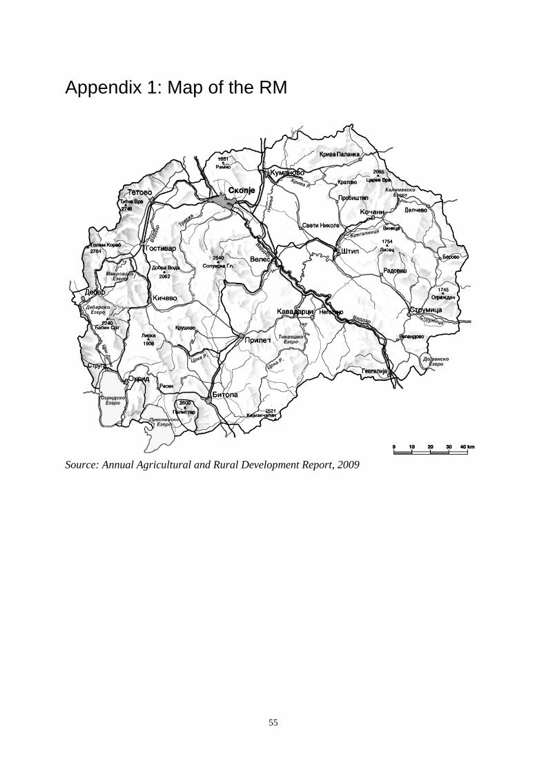
55

Appendix 1: Map of the RM

Source: Annual Agricultural and Rural Development Report, 2009

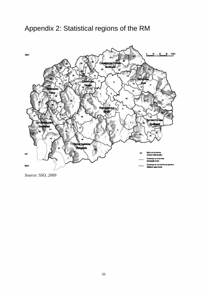
56

Appendix 2: Statistical regions of the RM

Source: SSO, 2009

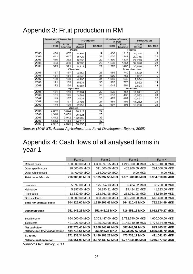
57

Appendix 3: Fruit production in RM

Source: (MAFWE, Annual Agricultural and Rural Development Report, 2009)

Appendix 4: Cash flows of all analysed farms in year 1 Farm 1 Farm 2 Farm 3 Farm 4 Material costs 180.000,00 MKD 1.380.397,55 MKD 1.219.500,00 MKD 2.690.010,00 MKD Other specific costs 28.500,00 MKD 311.000,00 MKD 462.200,00 MKD 294.000,00 MKD Other running costs 8.400,00 MKD 114.000,00 MKD 0,00 MKD 0,00 MKD Total material costs 216.900,00 MKD 1.805.397,55 MKD 1.681.700,00 MKD 2.984.010,00 MKD Insurance 5.397,00 MKD 175.954,13 MKD 36.424,22 MKD 68.250,30 MKD Maintance 5.397,00 MKD 66.890,31 MKD 19.424,22 MKD 41.223,60 MKD Profit taxes 13.532,60 MKD 253.761,98 MKD 253.761,98 MKD 64.650,59 MKD Gross salaries 180.000,00 MKD 833.200,00 MKD 355.200,00 MKD 618.400,00 MKD Total non-material costs 204.326,60 MKD 1.329.806,43 MKD 664.810,42 MKD 792.524,49 MKD Beginning cash 251.945,25 MKD 251.945,25 MKD 716.458,16 MKD 1.012.170,27 MKD Total income 654.000,00 MKD 6.303.447,00 MKD 2.732.790,00 MKD 4.600.000,00 MKD Total costs 421.226,60 MKD 3.135.203,98 MKD 2.145.340,49 MKD 3.776.534,49 MKD Net cash flow 232.773,40 MKD 3.168.243,02 MKD 587.449,51 MKD 823.465,52 MKD Balance non-financial operation 484.718,65 MKD 251.945,25 MKD 1.303.907,67 MKD 1.835.635,79 MKD EU grant 171.333,34 MKD 3.420.188,27 MKD 473.738,17 MKD 411.041,83 MKD Balance final operation 656.051,99 MKD 3.672.133.52 MKD 1.777.645,84 MKD 2.246.677,62 MKD

Source: Own survey, 2011

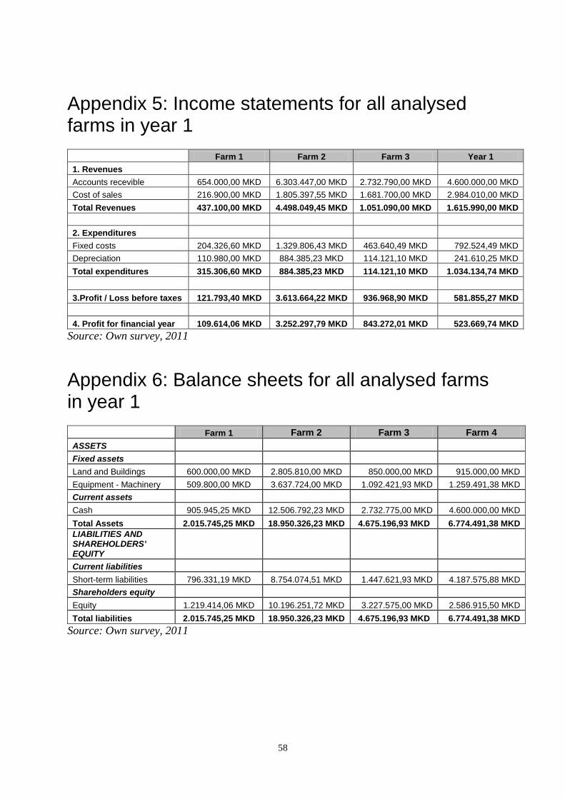
58

Appendix 5: Income statements for all analysed farms in year 1

Farm 1 Farm 2 Farm 3 Year 1 1. Revenues Accounts recevible 654.000,00 MKD 6.303.447,00 MKD 2.732.790,00 MKD 4.600.000,00 MKD Cost of sales 216.900,00 MKD 1.805.397,55 MKD 1.681.700,00 MKD 2.984.010,00 MKD Total Revenues 437.100,00 MKD 4.498.049,45 MKD 1.051.090,00 MKD 1.615.990,00 MKD 2. Expenditures Fixed costs 204.326,60 MKD 1.329.806,43 MKD 463.640,49 MKD 792.524,49 MKD Depreciation 110.980,00 MKD 884.385,23 MKD 114.121,10 MKD 241.610,25 MKD Total expenditures 315.306,60 MKD 884.385,23 MKD 114.121,10 MKD 1.034.134,74 MKD 3.Profit / Loss before taxes 121.793,40 MKD 3.613.664,22 MKD 936.968,90 MKD 581.855,27 MKD 4. Profit for financial year 109.614,06 MKD 3.252.297,79 MKD 843.272,01 MKD 523.669,74 MKD

Source: Own survey, 2011

Appendix 6: Balance sheets for all analysed farms in year 1

Farm 1 Farm 2 Farm 3 Farm 4 ASSETS Fixed assets Land and Buildings 600.000,00 MKD 2.805.810,00 MKD 850.000,00 MKD 915.000,00 MKD Equipment - Machinery 509.800,00 MKD 3.637.724,00 MKD 1.092.421,93 MKD 1.259.491,38 MKD Current assets Cash 905.945,25 MKD 12.506.792,23 MKD 2.732.775,00 MKD 4.600.000,00 MKD Total Assets 2.015.745,25 MKD 18.950.326,23 MKD 4.675.196,93 MKD 6.774.491,38 MKD LIABILITIES AND SHAREHOLDERS' EQUITY Current liabilities Short-term liabilities 796.331,19 MKD 8.754.074,51 MKD 1.447.621,93 MKD 4.187.575,88 MKD Shareholders equity Equity 1.219.414,06 MKD 10.196.251,72 MKD 3.227.575,00 MKD 2.586.915,50 MKD Total liabilities 2.015.745,25 MKD 18.950.326,23 MKD 4.675.196,93 MKD 6.774.491,38 MKD

Source: Own survey, 2011

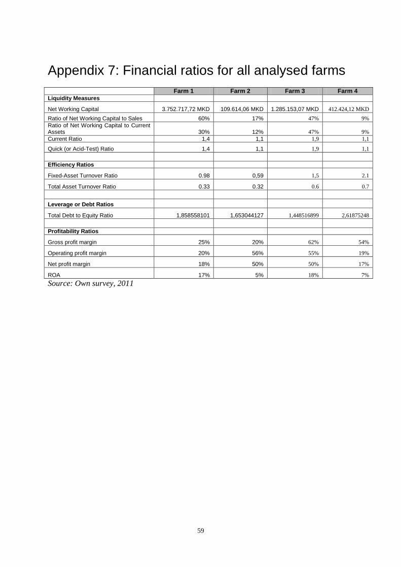
59

Appendix 7: Financial ratios for all analysed farms Farm 1 Farm 2 Farm 3 Farm 4 Liquidity Measures

Net Working Capital 3.752.717,72 MKD 109.614,06 MKD 1.285.153,07 MKD 412.424,12 MKD Ratio of Net Working Capital to Sales 60% 17% 47% 9% Ratio of Net Working Capital to Current Assets 30% 12% 47% 9% Current Ratio 1,4 1,1 1,9 1,1

Quick (or Acid-Test) Ratio 1,4 1,1 1,9 1,1 Efficiency Ratios

Fixed-Asset Turnover Ratio 0.98 0,59 1,5 2.1

Total Asset Turnover Ratio 0.33 0.32 0.6 0.7 Leverage or Debt Ratios

Total Debt to Equity Ratio 1,858558101 1,653044127 1,448516899 2,61875248 Profitability Ratios

Gross profit margin 25% 20% 62% 54%

Operating profit margin 20% 56% 55% 19%

Net profit margin 18% 50% 50% 17%

ROA 17% 5% 18% 7% Source: Own survey, 2011

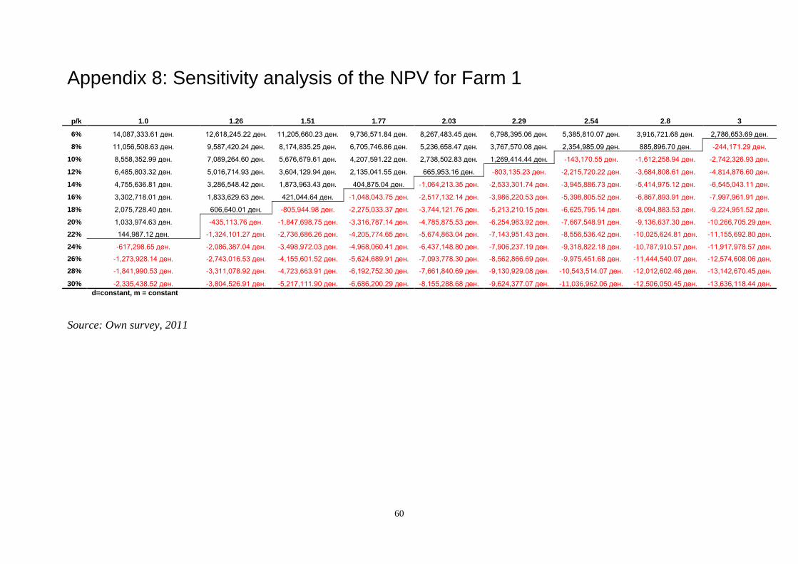
60

Appendix 8: Sensitivity analysis of the NPV for Farm 1

p/k 1.0 1.26 1.51 1.77 2.03 2.29 2.54 2.8 3

6% 14,087,333.61 ден. 12,618,245.22 ден. 11,205,660.23 ден. 9,736,571.84 ден. 8,267,483.45 ден. 6,798,395.06 ден. 5,385,810.07 ден. 3,916,721.68 ден. 2,786,653.69 ден.

8% 11,056,508.63 ден. 9,587,420.24 ден. 8,174,835.25 ден. 6,705,746.86 ден. 5,236,658.47 ден. 3,767,570.08 ден. 2,354,985.09 ден. 885,896.70 ден. -244,171.29 ден.

10% 8,558,352.99 ден. 7,089,264.60 ден. 5,676,679.61 ден. 4,207,591.22 ден. 2,738,502.83 ден. 1,269,414.44 ден. -143,170.55 ден. -1,612,258.94 ден. -2,742,326.93 ден.

12% 6,485,803.32 ден. 5,016,714.93 ден. 3,604,129.94 ден. 2,135,041.55 ден. 665,953.16 ден. -803,135.23 ден. -2,215,720.22 ден. -3,684,808.61 ден. -4,814,876.60 ден.

14% 4,755,636.81 ден. 3,286,548.42 ден. 1,873,963.43 ден. 404,875.04 ден. -1,064,213.35 ден. -2,533,301.74 ден. -3,945,886.73 ден. -5,414,975.12 ден. -6,545,043.11 ден.

16% 3,302,718.01 ден. 1,833,629.63 ден. 421,044.64 ден. -1,048,043.75 ден. -2,517,132.14 ден. -3,986,220.53 ден. -5,398,805.52 ден. -6,867,893.91 ден. -7,997,961.91 ден.

18% 2,075,728.40 ден. 606,640.01 ден. -805,944.98 ден. -2,275,033.37 ден. -3,744,121.76 ден. -5,213,210.15 ден. -6,625,795.14 ден. -8,094,883.53 ден. -9,224,951.52 ден.

20% 1,033,974.63 ден. -435,113.76 ден. -1,847,698.75 ден. -3,316,787.14 ден. -4,785,875.53 ден. -6,254,963.92 ден. -7,667,548.91 ден. -9,136,637.30 ден. -10,266,705.29 ден.

22% 144,987.12 ден. -1,324,101.27 ден. -2,736,686.26 ден. -4,205,774.65 ден. -5,674,863.04 ден. -7,143,951.43 ден. -8,556,536.42 ден. -10,025,624.81 ден. -11,155,692.80 ден.

24% -617,298.65 ден. -2,086,387.04 ден. -3,498,972.03 ден. -4,968,060.41 ден. -6,437,148.80 ден. -7,906,237.19 ден. -9,318,822.18 ден. -10,787,910.57 ден. -11,917,978.57 ден.

26% -1,273,928.14 ден. -2,743,016.53 ден. -4,155,601.52 ден. -5,624,689.91 ден. -7,093,778.30 ден. -8,562,866.69 ден. -9,975,451.68 ден. -11,444,540.07 ден. -12,574,608.06 ден.

28% -1,841,990.53 ден. -3,311,078.92 ден. -4,723,663.91 ден. -6,192,752.30 ден. -7,661,840.69 ден. -9,130,929.08 ден. -10,543,514.07 ден. -12,012,602.46 ден. -13,142,670.45 ден.

30% -2,335,438.52 ден. -3,804,526.91 ден. -5,217,111.90 ден. -6,686,200.29 ден. -8,155,288.68 ден. -9,624,377.07 ден. -11,036,962.06 ден. -12,506,050.45 ден. -13,636,118.44 ден.

d=constant, m = constant

Source: Own survey, 2011

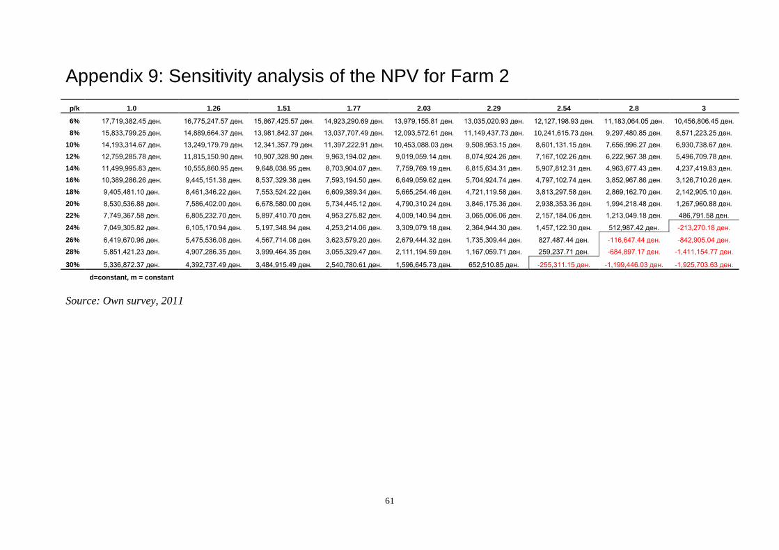
61

Appendix 9: Sensitivity analysis of the NPV for Farm 2 p/k 1.0 1.26 1.51 1.77 2.03 2.29 2.54 2.8 3

6% 17,719,382.45 ден. 16,775,247.57 ден. 15,867,425.57 ден. 14,923,290.69 ден. 13,979,155.81 ден. 13,035,020.93 ден. 12,127,198.93 ден. 11,183,064.05 ден. 10,456,806.45 ден.

8% 15,833,799.25 ден. 14,889,664.37 ден. 13,981,842.37 ден. 13,037,707.49 ден. 12,093,572.61 ден. 11,149,437.73 ден. 10,241,615.73 ден. 9,297,480.85 ден. 8,571,223.25 ден.

10% 14,193,314.67 ден. 13,249,179.79 ден. 12,341,357.79 ден. 11,397,222.91 ден. 10,453,088.03 ден. 9,508,953.15 ден. 8,601,131.15 ден. 7,656,996.27 ден. 6,930,738.67 ден.

12% 12,759,285.78 ден. 11,815,150.90 ден. 10,907,328.90 ден. 9,963,194.02 ден. 9,019,059.14 ден. 8,074,924.26 ден. 7,167,102.26 ден. 6,222,967.38 ден. 5,496,709.78 ден.

14% 11,499,995.83 ден. 10,555,860.95 ден. 9,648,038.95 ден. 8,703,904.07 ден. 7,759,769.19 ден. 6,815,634.31 ден. 5,907,812.31 ден. 4,963,677.43 ден. 4,237,419.83 ден.

16% 10,389,286.26 ден. 9,445,151.38 ден. 8,537,329.38 ден. 7,593,194.50 ден. 6,649,059.62 ден. 5,704,924.74 ден. 4,797,102.74 ден. 3,852,967.86 ден. 3,126,710.26 ден.

18% 9,405,481.10 ден. 8,461,346.22 ден. 7,553,524.22 ден. 6,609,389.34 ден. 5,665,254.46 ден. 4,721,119.58 ден. 3,813,297.58 ден. 2,869,162.70 ден. 2,142,905.10 ден.

20% 8,530,536.88 ден. 7,586,402.00 ден. 6,678,580.00 ден. 5,734,445.12 ден. 4,790,310.24 ден. 3,846,175.36 ден. 2,938,353.36 ден. 1,994,218.48 ден. 1,267,960.88 ден.

22% 7,749,367.58 ден. 6,805,232.70 ден. 5,897,410.70 ден. 4,953,275.82 ден. 4,009,140.94 ден. 3,065,006.06 ден. 2,157,184.06 ден. 1,213,049.18 ден. 486,791.58 ден.

24% 7,049,305.82 ден. 6,105,170.94 ден. 5,197,348.94 ден. 4,253,214.06 ден. 3,309,079.18 ден. 2,364,944.30 ден. 1,457,122.30 ден. 512,987.42 ден. -213,270.18 ден.

26% 6,419,670.96 ден. 5,475,536.08 ден. 4,567,714.08 ден. 3,623,579.20 ден. 2,679,444.32 ден. 1,735,309.44 ден. 827,487.44 ден. -116,647.44 ден. -842,905.04 ден.

28% 5,851,421.23 ден. 4,907,286.35 ден. 3,999,464.35 ден. 3,055,329.47 ден. 2,111,194.59 ден. 1,167,059.71 ден. 259,237.71 ден. -684,897.17 ден. -1,411,154.77 ден.

30% 5,336,872.37 ден. 4,392,737.49 ден. 3,484,915.49 ден. 2,540,780.61 ден. 1,596,645.73 ден. 652,510.85 ден. -255,311.15 ден. -1,199,446.03 ден. -1,925,703.63 ден.

d=constant, m = constant

Source: Own survey, 2011

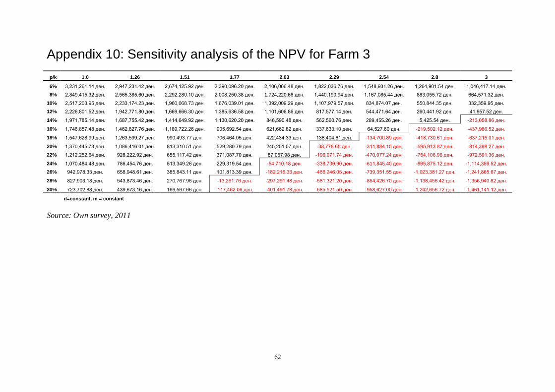
62

Appendix 10: Sensitivity analysis of the NPV for Farm 3 p/k 1.0 1.26 1.51 1.77 2.03 2.29 2.54 2.8 3

6% 3,231,261.14 ден. 2,947,231.42 ден. 2,674,125.92 ден. 2,390,096.20 ден. 2,106,066.48 ден. 1,822,036.76 ден. 1,548,931.26 ден. 1,264,901.54 ден. 1,046,417.14 ден.

8% 2,849,415.32 ден. 2,565,385.60 ден. 2,292,280.10 ден. 2,008,250.38 ден. 1,724,220.66 ден. 1,440,190.94 ден. 1,167,085.44 ден. 883,055.72 ден. 664,571.32 ден.

10% 2,517,203.95 ден. 2,233,174.23 ден. 1,960,068.73 ден. 1,676,039.01 ден. 1,392,009.29 ден. 1,107,979.57 ден. 834,874.07 ден. 550,844.35 ден. 332,359.95 ден.

12% 2,226,801.52 ден. 1,942,771.80 ден. 1,669,666.30 ден. 1,385,636.58 ден. 1,101,606.86 ден. 817,577.14 ден. 544,471.64 ден. 260,441.92 ден. 41,957.52 ден.

14% 1,971,785.14 ден. 1,687,755.42 ден. 1,414,649.92 ден. 1,130,620.20 ден. 846,590.48 ден. 562,560.76 ден. 289,455.26 ден. 5,425.54 ден. -213,058.86 ден.

16% 1,746,857.48 ден. 1,462,827.76 ден. 1,189,722.26 ден. 905,692.54 ден. 621,662.82 ден. 337,633.10 ден. 64,527.60 ден. -219,502.12 ден. -437,986.52 ден.

18% 1,547,628.99 ден. 1,263,599.27 ден. 990,493.77 ден. 706,464.05 ден. 422,434.33 ден. 138,404.61 ден. -134,700.89 ден. -418,730.61 ден. -637,215.01 ден.

20% 1,370,445.73 ден. 1,086,416.01 ден. 813,310.51 ден. 529,280.79 ден. 245,251.07 ден. -38,778.65 ден. -311,884.15 ден. -595,913.87 ден. -814,398.27 ден.

22% 1,212,252.64 ден. 928,222.92 ден. 655,117.42 ден. 371,087.70 ден. 87,057.98 ден. -196,971.74 ден. -470,077.24 ден. -754,106.96 ден. -972,591.36 ден.

24% 1,070,484.48 ден. 786,454.76 ден. 513,349.26 ден. 229,319.54 ден. -54,710.18 ден. -338,739.90 ден. -611,845.40 ден. -895,875.12 ден. -1,114,359.52 ден.

26% 942,978.33 ден. 658,948.61 ден. 385,843.11 ден. 101,813.39 ден. -182,216.33 ден. -466,246.05 ден. -739,351.55 ден. -1,023,381.27 ден. -1,241,865.67 ден.

28% 827,903.18 ден. 543,873.46 ден. 270,767.96 ден. -13,261.76 ден. -297,291.48 ден. -581,321.20 ден. -854,426.70 ден. -1,138,456.42 ден. -1,356,940.82 ден.

30% 723,702.88 ден. 439,673.16 ден. 166,567.66 ден. -117,462.06 ден. -401,491.78 ден. -685,521.50 ден. -958,627.00 ден. -1,242,656.72 ден. -1,461,141.12 ден.

d=constant, m = constant Source: Own survey, 2011

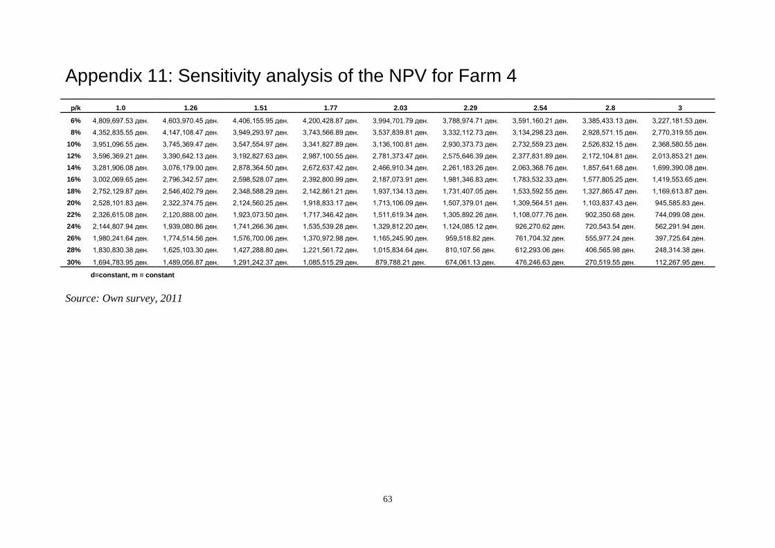
63

Appendix 11: Sensitivity analysis of the NPV for Farm 4

p/k 1.0 1.26 1.51 1.77 2.03 2.29 2.54 2.8 3

6% 4,809,697.53 ден. 4,603,970.45 ден. 4,406,155.95 ден. 4,200,428.87 ден. 3,994,701.79 ден. 3,788,974.71 ден. 3,591,160.21 ден. 3,385,433.13 ден. 3,227,181.53 ден.

8% 4,352,835.55 ден. 4,147,108.47 ден. 3,949,293.97 ден. 3,743,566.89 ден. 3,537,839.81 ден. 3,332,112.73 ден. 3,134,298.23 ден. 2,928,571.15 ден. 2,770,319.55 ден.

10% 3,951,096.55 ден. 3,745,369.47 ден. 3,547,554.97 ден. 3,341,827.89 ден. 3,136,100.81 ден. 2,930,373.73 ден. 2,732,559.23 ден. 2,526,832.15 ден. 2,368,580.55 ден.

12% 3,596,369.21 ден. 3,390,642.13 ден. 3,192,827.63 ден. 2,987,100.55 ден. 2,781,373.47 ден. 2,575,646.39 ден. 2,377,831.89 ден. 2,172,104.81 ден. 2,013,853.21 ден.

14% 3,281,906.08 ден. 3,076,179.00 ден. 2,878,364.50 ден. 2,672,637.42 ден. 2,466,910.34 ден. 2,261,183.26 ден. 2,063,368.76 ден. 1,857,641.68 ден. 1,699,390.08 ден.

16% 3,002,069.65 ден. 2,796,342.57 ден. 2,598,528.07 ден. 2,392,800.99 ден. 2,187,073.91 ден. 1,981,346.83 ден. 1,783,532.33 ден. 1,577,805.25 ден. 1,419,553.65 ден.

18% 2,752,129.87 ден. 2,546,402.79 ден. 2,348,588.29 ден. 2,142,861.21 ден. 1,937,134.13 ден. 1,731,407.05 ден. 1,533,592.55 ден. 1,327,865.47 ден. 1,169,613.87 ден.

20% 2,528,101.83 ден. 2,322,374.75 ден. 2,124,560.25 ден. 1,918,833.17 ден. 1,713,106.09 ден. 1,507,379.01 ден. 1,309,564.51 ден. 1,103,837.43 ден. 945,585.83 ден.

22% 2,326,615.08 ден. 2,120,888.00 ден. 1,923,073.50 ден. 1,717,346.42 ден. 1,511,619.34 ден. 1,305,892.26 ден. 1,108,077.76 ден. 902,350.68 ден. 744,099.08 ден.

24% 2,144,807.94 ден. 1,939,080.86 ден. 1,741,266.36 ден. 1,535,539.28 ден. 1,329,812.20 ден. 1,124,085.12 ден. 926,270.62 ден. 720,543.54 ден. 562,291.94 ден.

26% 1,980,241.64 ден. 1,774,514.56 ден. 1,576,700.06 ден. 1,370,972.98 ден. 1,165,245.90 ден. 959,518.82 ден. 761,704.32 ден. 555,977.24 ден. 397,725.64 ден.

28% 1,830,830.38 ден. 1,625,103.30 ден. 1,427,288.80 ден. 1,221,561.72 ден. 1,015,834.64 ден. 810,107.56 ден. 612,293.06 ден. 406,565.98 ден. 248,314.38 ден.

30% 1,694,783.95 ден. 1,489,056.87 ден. 1,291,242.37 ден. 1,085,515.29 ден. 879,788.21 ден. 674,061.13 ден. 476,246.63 ден. 270,519.55 ден. 112,267.95 ден.

d=constant, m = constant

Source: Own survey, 2011

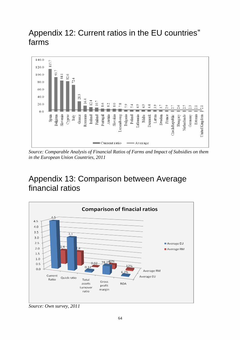
64

Appendix 12: Current ratios in the EU countries‟ farms

Source: Comparable Analysis of Financial Ratios of Farms and Impact of Subsidies on them in the European Union Countries, 2011

Appendix 13: Comparison between Average financial ratios

Source: Own survey, 2011