Embed Size (px)
Citation preview
Sensitivity Analysis and Least Squares Parameter Estimation for an Epidemic Model
Alun L. Lloyd
Department of MathematicsBiomathematics Graduate Program
Center for Quantitative Sciences in BiomedicineNorth Carolina State University
Aims of this Practical1. Learn about simple epidemic model, how it behaves and how to simulate it
2. Derive sensitivity equations for the model
3. Fit the model to data from an outbreak, estimating model parameters
4. Obtain measures of uncertainty for these estimated parameters
Aims of this Practical1. Learn about simple epidemic model, how it behaves and how to simulate it
simulating differential equation models in MATLAB2. Derive sensitivity equations for the model
3. Fit the model to data from an outbreak, estimating model parametersminimizing a function in MATLAB
4. Obtain measures of uncertainty for these estimated parameters

SIR Model for Spread of Infection
Compartmental model: Susceptibles, Infectives, Recovereds
Ignore births and deaths (e.g. short-lived outbreak)“Standard incidence” term bSI/N b : “transmission parameter”
“well-mixed” populationAssume constant per-capita recovery rate of g
1/g is average duration of infectiousness
Note: S + I + R = N (constant), so need only worry about S and I
Sensitivity of Model-Based Epidemiological Parameter Estimation 125
of transmission within families, or other transmission experiments. Such data,however, are often unavailable during the early stages of a disease outbreak.
An alternative approach involves fitting a mathematical model to outbreak data,obtaining estimates for the parameters of the model, allowing R0 to be calculated.The simplest model that can be used for this purpose is the standard deterministiccompartmental SIR model [see, for example, 11]. Individuals are assumed to eitherbe susceptible, infectious or removed, with the numbers of each being written asS, I , and R, respectively. Susceptible individuals acquire infection through con-tacts with infectious individuals, and the simplest form of the model assumes thatnew infections arise at rate βSI/N . Here N is the population size and β is thetransmission parameter, which is given by the product of the contact rate and thetransmission probability. Recovery of infectives is assumed to occur at a constantrate γ , corresponding to an average duration of infection of 1/γ , and leads to per-manent immunity. Throughout this chapter we shall denote the average duration ofinfectiousness by DI and assume permanent immunity following infection. We shallalso ignore demographic processes (births and deaths), which is a good approxi-mation if the disease outbreak is short-lived and the infection is non-fatal. Ignoringdemography leads to the population size N being constant. The model can be writtenas the following set of differential equations
dS/dt = −βSI/N (1)
dI/dt = βSI/N − γ I (2)
dR/dt = γ I. (3)
During the early stages of an outbreak with a novel pathogen, almost the entirepopulation will be susceptible, and, since S ≈ N , the transmission rate equalsβ I . The transmission parameter β is the rate at which each infective gives riseto secondary infections and so the basic reproductive number can be written asR0 = βDI = β/γ . During this initial period, the changing prevalence of infec-tion can, to a very good approximation, be described by the single linear equationd I/dt = γ (R0 − 1)I. (We remark that the S = N assumption corresponds tolinearizing the model about its infection free equilibrium.) In other words, providedthat R0 is greater than one, which we shall assume to be the case throughout thischapter, prevalence initially increases exponentially with growth rate
r = γ (R0 − 1). (4)
The incidence of infection is given by βSI/N and so, during the early stages ofan outbreak, prevalence and incidence are proportional in the SIR setting, so thisequation also describes the rate at which incidence grows.
Equation (4) provides a relationship, R0 = 1 + r DI, between R0 and quan-tities that can typically be measured (the initial growth rate of the epidemic andthe average duration of infection), and as a result has provided one of the moststraightforward ways to estimate R0.
y0 1
Figure 6: Direction field for the SI model. The arrows show the direction in which y moves: y willincrease if it lies between 0 and 1.
6 Describing Recovery from Infection and Disease Outbreaks: The
SIR Model in a Closed Population
Typically, people do not remain infectious: they recover or die. We can model this by including a‘removed’ class in the model, leading to an SIR model.
IS Rinfection recovery
Figure 7: Flowchart showing movement between classes in the SIR model.
We have to describe the I to R transition in some way. The simplest assumption takes the recovery(removal) term to be proportional to the number of infective individuals:
S = ��SI/N (15)
I = �SI/N � �I (16)
R = �I. (17)
Again, we consider a closed population, so S + I + R = N . We usually consider the initial numberof susceptibles to be close to N .
This model is often called the Kermack and McKendrick model as it appeared in their 1927 paper.It is also called the general epidemic model. (Although this SIR model is often called THEKermack and McKendrick model, it has been pointed out that the 1927 paper goes beyond thismodel, discussing a more general framework that employs fewer assumptions.)
It’s worth pausing to think about the assumption made regarding the recovery term. Having aconstant recovery rate means that the distribution of infectious periods is exponential with mean1/�. Biologically, this assumption corresponds to the chance of recovery being independent ofthe time since infection. In most cases this is far from realistic, but it considerably simplifies the
16
Behavior of SIR Model
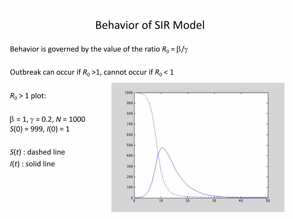
Behavior is governed by the value of the ratio R0 = b/g
Outbreak can occur if R0 >1, cannot occur if R0 < 1
R0 > 1 plot:
b = 1, g = 0.2, N = 1000S(0) = 999, I(0) = 1
S(t) : dashed lineI(t) : solid line
Behavior of SIR Model
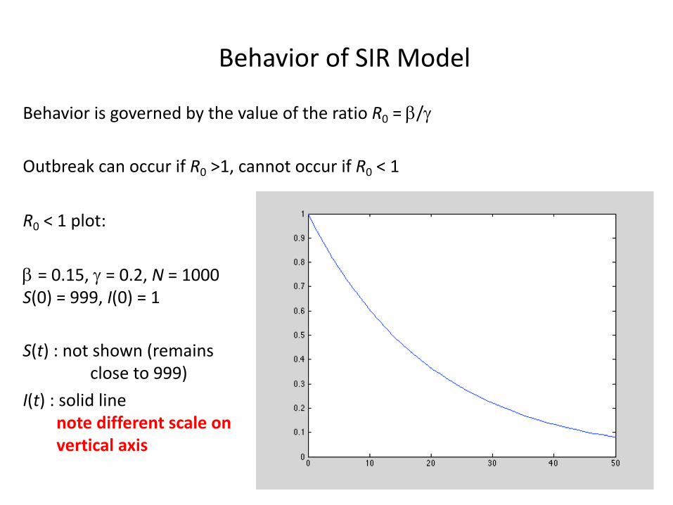
Behavior is governed by the value of the ratio R0 = b/g
Outbreak can occur if R0 >1, cannot occur if R0 < 1
R0 < 1 plot:
b = 0.15, g = 0.2, N = 1000S(0) = 999, I(0) = 1
S(t) : not shown (remainsclose to 999)
I(t) : solid linenote different scale on vertical axis

Simple Analysis of SIR Model in Terms of R0
Consider dI/dt :
(*)
per-capita transmission maximized when S ≈ N :
I increases if R0 >1, decreases if R0 < 1
R0 : basic reproductive number = b x 1/g = b x (av. duration of infection)
average number of secondary infections caused by an infectious individual when the population is almost entirely susceptible
dI
dt= �SI/N � �I
= �
✓�
�
S
N� 1
◆I
= � (R0{S/N}� 1) I
dI
dt= � (R0 � 1) I
Epidemiological Importance of R0
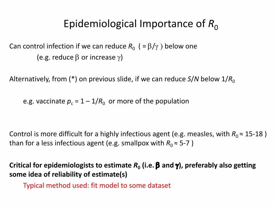
Can control infection if we can reduce R0 ( = b/g ) below one (e.g. reduce b or increase g)
Alternatively, from (*) on previous slide, if we can reduce S/N below 1/R0
e.g. vaccinate pc = 1 – 1/R0 or more of the population
Control is more difficult for a highly infectious agent (e.g. measles, with R0 ≈ 15-18 ) than for a less infectious agent (e.g. smallpox with R0 ≈ 5-7 )
Critical for epidemiologists to estimate R0 (i.e. b and g), preferably also getting some idea of reliability of estimate(s)
Typical method used: fit model to some dataset
The Data
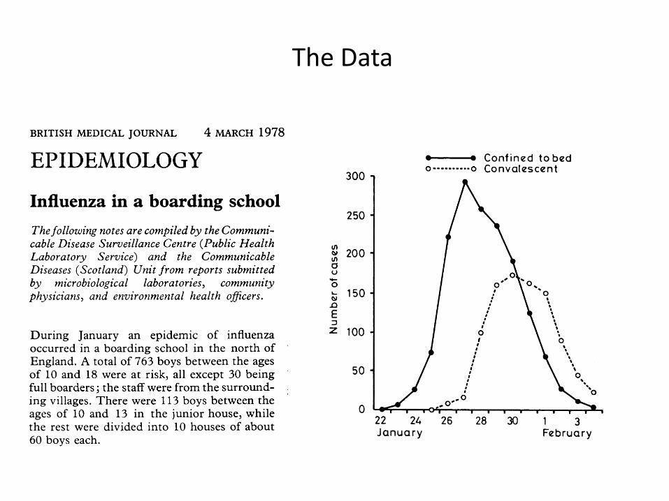
587BRITISH MEDICAL JOURNAL 4 MARCH 1978
EPIDEMIOLOGY
Influenza in a boarding schoolThefollowing notes are compiled by the Communi-cable Disease Surveillance Centre (Public HealthLaboratory Service) and the CommunicableDiseases (Scotland) Unit from reports submittedby microbiological laboratories, communityphysicians, and environmental health officers.
During January an epidemic of influenzaoccurred in a boarding school in the north ofEngland. A total of 763 boys between the agesof 10 and 18 were at risk, all except 30 beingfull boarders; the staff were from the surround-ing villages. There were 113 boys between theages of 10 and 13 in the junior house, whilethe rest were divided into 10 houses of about60 boys each.The Easter term began on 10 January, with
boys returning from all over Britain and somefrom Europe and the Far East. One boy fromHong Kong had a transient febrile illnessfrom 15 to 18 January. On Sunday 22 Januarythree boys were in the college infirmary. Thegraph shows the daily total number confinedto bed or convalescent during the epidemic:512 boys (67° 0) spent between three and sevendays away from class, and 83 of the boys inthe junior house were affected. Of about 130adults who had some contact with the boys,only one, a house matron, developed similarsymptoms.Most of the boys who became ill first com-
plained of feeling very tired, with headache asfever developed, and sore throat and tracheitisbeing the rule. The temperature was usually100--102'F (38° -39-C) and often higher in themorning. Three boys with no other abnormal
300
250
U,w 200a0
, 150nEZ 100
50
0
0--
22 24January
signs had temper;41° C). Many haanterior pillars ofnever looked as i:gested. In only fivlsigns on chest ex;sided quickly oncebed. They weretheir temperaturesback to classes twoon the severity of toff sick was five toOne boy of 13
days with probablea temperature of1 10/min, respiratic
- Confined to bed sounds in his right lung. He was given.-0----o Convalescent ampicillin and by next morning his tempera-
ture was 99° F (37° C) and his chest clear. Fivedays later he went home to convalesce. Fourboys developed wheezy bronchitis. Tworeceived ampicillin and two tetracycline. Allrecovered quickly and were back at work inseven to eight days. Four boys with otitis
| media, with bulging red ear drums, respondedto ampicillin within 48 hours and none hadany aural discharge. One boy had sinusitis,which again responded to ampicillin. He wasin bed for seven days and off work for ten days.In all, only 10 of the 512 boys who became illreceived antibiotics.
Throat swabs were taken from eight boys,and influenza A viruses similar to A/USSR/90/
01. 0 77 (HlN1) were isolated from six. The spread'26 ' 28' - l '3 - of this virus through the school was much
Februo3ry more rapid than in the outbreaks due to in-fluenza B in November 1954 and to influenza A
atures of 1050-106° F (40° - (Asian flu) H2N2 in October 1957. These twod mild reddening of the epidemics reached their peak in two weeks andthe fauces, but the throat lasted four weeks. This year's epidemicnflamed as symptoms sug- reached a peak in seven days and was over ine boys were there abnormal 13 days. Influenza vaccine (Fluvirin) had beenamination. Symptoms sub- given to 630 boys in October 1977-as hadthe boys were confined to been the practice for some years. The inci-
allowed up 36 hours after dence of influenza among the boys had beenhad returned to normal and low except in those years in which a definiteto four days later, depending antigenic shift occurred. The fact that this isthe attack. The average time the first major outbreak of influenza at thesix days. school since the Asian flu suggests that in-was readmitted after two fluenza vaccination has a useful role in a board-
e bacterial pneumonia, with ing school. Had it been possible to include the104° F (40° C), pulse rate of HlNl strain in the vaccine a major outbreakn rate of 22/min, and moist might well have been avoided.
PARLIAMENT
Abortion (Amendment) BillSir Bernard Braine introduced a Bill on
21 February "to make further provision withrespect to the protection of the life of a viablefetus; to amend section 4 of the Abortion Act1967; to regulate the provision of payment forconsultation and advice in relation to thetermination of pregnancy; and to make pro-vision with respect to bodies corporate." Heemphasised that the Bill was limited solely tothree important matters of principle and wouldnot interfere "in any way with the criteria forlawful abortion laid down in the 1967 Act."The first change he wanted was to reduce theupper limit for an abortion from 28 to 20weeks. The BMA, the Peel Advisory Group,Sir Stanley Clayton (when president of theRCOG), and a poll among gynaecologists hadall favoured a 20-week limit or less.The Bill's second purpose was to strengthen
and clarify the provision in section 4 of the1967 Act regarding conscientious objection totaking part in an abortion by giving statutoryclarification of the grounds on which objec-tion could be based. The third change wouldrequire all pregnancy advisory bureaux whichcharged fees to be licensed by the Secretary ofState, as proposed by the Lane Committee.
A condition of licensing would be that thebureaux should have no financial connectionwith abortion clinics. Sir Bernard admittedthat without the Government's help the Billwas unlikely to make progress.
Opposition to Bill
Sir George Sinclair opposed the Bill be-cause, he said, "it would pave the way for aBill to restrict the operation of the 1967 Act,and because it is in the teeth of the medicalprofession." It was only in the most excep-tional cases that abortion after 20 weeks wassanctioned. Furthermore, "until, in certainareas, the restrictions under the NHS areremoved, and with them the risk of delay, itwould, in my view, be too soon to change theexisting time limit." But, most importantly,to disrupt the services of the British PregnancyAdvisory Service and the Pregnancy AdvisoryService in London, which the Bill sought todo, would "once again drive women ... to backstreet abortions." Half of all abortions werestill carried out in the private sector. TheBMA, Sir George said, had voted against anyamendment to the 1967 Act at its 1977 ARM."I hope," he concluded, "that in view of themedical opinion and the need of women indistress, the motion will be given very littlesupport."The Bill was given a first reading by 181
votes to 175.
Medical BillThe Medical Bill was considered by a
second reading committee in the House ofCommons on 22 February. The Minister ofState, Mr Roland Moyle, explained the Billclause by clause and told the committee of theamendments which had been made in theHouse of Lords (4 February, p 311). "TheBill," he said, "is no longer a short first-stagemeasure. It is considerably longer than it wason its original introduction. The reason is thata consensus on the additional provisions hasdeveloped more rapidly than at one time wasthought possible, and we want to meet thatconsensus in full. I hope that, during itspassage through the House, the Governmentand the committee will be able to make theBill even more comprehensive." The onlyoutstanding issue, which had been covered inthe Merrison Report, was the question ofspecialist registration.During the debate in the committee the size
and cost of the new council were raised. MrMoyle pointed out that the figure of 98 did notappear anywhere in the Bill, though he con-ceded that the council would be considerablyenlarged. On the question of cost, he said"there has been no decision in principle abouthow the future costs of the new GeneralMedical Council are to be met."The committee recommended that the Bill
should be read a second time and the Housegave the Bill a second reading on 23 February.
Fitting the SIR Model to Data
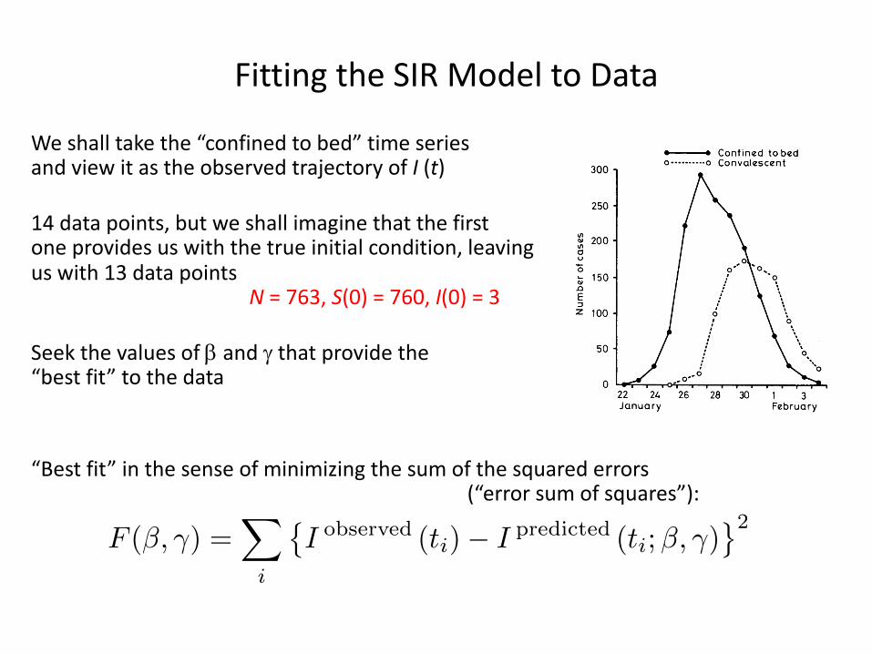
We shall take the “confined to bed” time seriesand view it as the observed trajectory of I (t)
14 data points, but we shall imagine that the firstone provides us with the true initial condition, leaving
us with 13 data pointsN = 763, S(0) = 760, I(0) = 3
Seek the values of b and g that provide the“best fit” to the data
“Best fit” in the sense of minimizing the sum of the squared errors (“error sum of squares”):
587BRITISH MEDICAL JOURNAL 4 MARCH 1978
EPIDEMIOLOGY
Influenza in a boarding schoolThefollowing notes are compiled by the Communi-cable Disease Surveillance Centre (Public HealthLaboratory Service) and the CommunicableDiseases (Scotland) Unit from reports submittedby microbiological laboratories, communityphysicians, and environmental health officers.
During January an epidemic of influenzaoccurred in a boarding school in the north ofEngland. A total of 763 boys between the agesof 10 and 18 were at risk, all except 30 beingfull boarders; the staff were from the surround-ing villages. There were 113 boys between theages of 10 and 13 in the junior house, whilethe rest were divided into 10 houses of about60 boys each.The Easter term began on 10 January, with
boys returning from all over Britain and somefrom Europe and the Far East. One boy fromHong Kong had a transient febrile illnessfrom 15 to 18 January. On Sunday 22 Januarythree boys were in the college infirmary. Thegraph shows the daily total number confinedto bed or convalescent during the epidemic:512 boys (67° 0) spent between three and sevendays away from class, and 83 of the boys inthe junior house were affected. Of about 130adults who had some contact with the boys,only one, a house matron, developed similarsymptoms.Most of the boys who became ill first com-
plained of feeling very tired, with headache asfever developed, and sore throat and tracheitisbeing the rule. The temperature was usually100--102'F (38° -39-C) and often higher in themorning. Three boys with no other abnormal
300
250
U,w 200a0
, 150nEZ 100
50
0
0--
22 24January
signs had temper;41° C). Many haanterior pillars ofnever looked as i:gested. In only fivlsigns on chest ex;sided quickly oncebed. They weretheir temperaturesback to classes twoon the severity of toff sick was five toOne boy of 13
days with probablea temperature of1 10/min, respiratic
- Confined to bed sounds in his right lung. He was given.-0----o Convalescent ampicillin and by next morning his tempera-
ture was 99° F (37° C) and his chest clear. Fivedays later he went home to convalesce. Fourboys developed wheezy bronchitis. Tworeceived ampicillin and two tetracycline. Allrecovered quickly and were back at work inseven to eight days. Four boys with otitis
| media, with bulging red ear drums, respondedto ampicillin within 48 hours and none hadany aural discharge. One boy had sinusitis,which again responded to ampicillin. He wasin bed for seven days and off work for ten days.In all, only 10 of the 512 boys who became illreceived antibiotics.
Throat swabs were taken from eight boys,and influenza A viruses similar to A/USSR/90/
01. 0 77 (HlN1) were isolated from six. The spread'26 ' 28' - l '3 - of this virus through the school was much
Februo3ry more rapid than in the outbreaks due to in-fluenza B in November 1954 and to influenza A
atures of 1050-106° F (40° - (Asian flu) H2N2 in October 1957. These twod mild reddening of the epidemics reached their peak in two weeks andthe fauces, but the throat lasted four weeks. This year's epidemicnflamed as symptoms sug- reached a peak in seven days and was over ine boys were there abnormal 13 days. Influenza vaccine (Fluvirin) had beenamination. Symptoms sub- given to 630 boys in October 1977-as hadthe boys were confined to been the practice for some years. The inci-
allowed up 36 hours after dence of influenza among the boys had beenhad returned to normal and low except in those years in which a definiteto four days later, depending antigenic shift occurred. The fact that this isthe attack. The average time the first major outbreak of influenza at thesix days. school since the Asian flu suggests that in-was readmitted after two fluenza vaccination has a useful role in a board-
e bacterial pneumonia, with ing school. Had it been possible to include the104° F (40° C), pulse rate of HlNl strain in the vaccine a major outbreakn rate of 22/min, and moist might well have been avoided.
PARLIAMENT
Abortion (Amendment) BillSir Bernard Braine introduced a Bill on
21 February "to make further provision withrespect to the protection of the life of a viablefetus; to amend section 4 of the Abortion Act1967; to regulate the provision of payment forconsultation and advice in relation to thetermination of pregnancy; and to make pro-vision with respect to bodies corporate." Heemphasised that the Bill was limited solely tothree important matters of principle and wouldnot interfere "in any way with the criteria forlawful abortion laid down in the 1967 Act."The first change he wanted was to reduce theupper limit for an abortion from 28 to 20weeks. The BMA, the Peel Advisory Group,Sir Stanley Clayton (when president of theRCOG), and a poll among gynaecologists hadall favoured a 20-week limit or less.The Bill's second purpose was to strengthen
and clarify the provision in section 4 of the1967 Act regarding conscientious objection totaking part in an abortion by giving statutoryclarification of the grounds on which objec-tion could be based. The third change wouldrequire all pregnancy advisory bureaux whichcharged fees to be licensed by the Secretary ofState, as proposed by the Lane Committee.
A condition of licensing would be that thebureaux should have no financial connectionwith abortion clinics. Sir Bernard admittedthat without the Government's help the Billwas unlikely to make progress.
Opposition to Bill
Sir George Sinclair opposed the Bill be-cause, he said, "it would pave the way for aBill to restrict the operation of the 1967 Act,and because it is in the teeth of the medicalprofession." It was only in the most excep-tional cases that abortion after 20 weeks wassanctioned. Furthermore, "until, in certainareas, the restrictions under the NHS areremoved, and with them the risk of delay, itwould, in my view, be too soon to change theexisting time limit." But, most importantly,to disrupt the services of the British PregnancyAdvisory Service and the Pregnancy AdvisoryService in London, which the Bill sought todo, would "once again drive women ... to backstreet abortions." Half of all abortions werestill carried out in the private sector. TheBMA, Sir George said, had voted against anyamendment to the 1967 Act at its 1977 ARM."I hope," he concluded, "that in view of themedical opinion and the need of women indistress, the motion will be given very littlesupport."The Bill was given a first reading by 181
votes to 175.
Medical BillThe Medical Bill was considered by a
second reading committee in the House ofCommons on 22 February. The Minister ofState, Mr Roland Moyle, explained the Billclause by clause and told the committee of theamendments which had been made in theHouse of Lords (4 February, p 311). "TheBill," he said, "is no longer a short first-stagemeasure. It is considerably longer than it wason its original introduction. The reason is thata consensus on the additional provisions hasdeveloped more rapidly than at one time wasthought possible, and we want to meet thatconsensus in full. I hope that, during itspassage through the House, the Governmentand the committee will be able to make theBill even more comprehensive." The onlyoutstanding issue, which had been covered inthe Merrison Report, was the question ofspecialist registration.During the debate in the committee the size
and cost of the new council were raised. MrMoyle pointed out that the figure of 98 did notappear anywhere in the Bill, though he con-ceded that the council would be considerablyenlarged. On the question of cost, he said"there has been no decision in principle abouthow the future costs of the new GeneralMedical Council are to be met."The committee recommended that the Bill
should be read a second time and the Housegave the Bill a second reading on 23 February.
F (�, �) =X
i
�I observed (ti)� I predicted (ti;�, �)
2
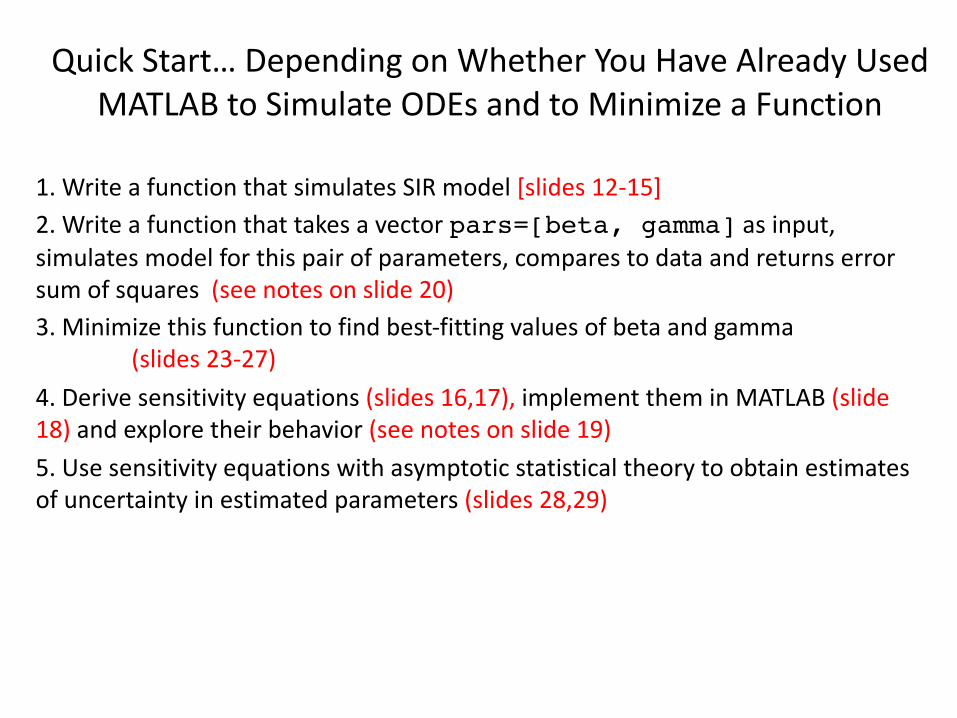
Quick Start… Depending on Whether You Have Already Used MATLAB to Simulate ODEs and to Minimize a Function
1. Write a function that simulates SIR model [slides 12-15]2. Write a function that takes a vector pars=[beta, gamma] as input, simulates model for this pair of parameters, compares to data and returns error sum of squares (see notes on slide 20)3. Minimize this function to find best-fitting values of beta and gamma
(slides 23-27)4. Derive sensitivity equations (slides 16,17), implement them in MATLAB (slide 18) and explore their behavior (see notes on slide 19)5. Use sensitivity equations with asymptotic statistical theory to obtain estimates of uncertainty in estimated parameters (slides 28,29)
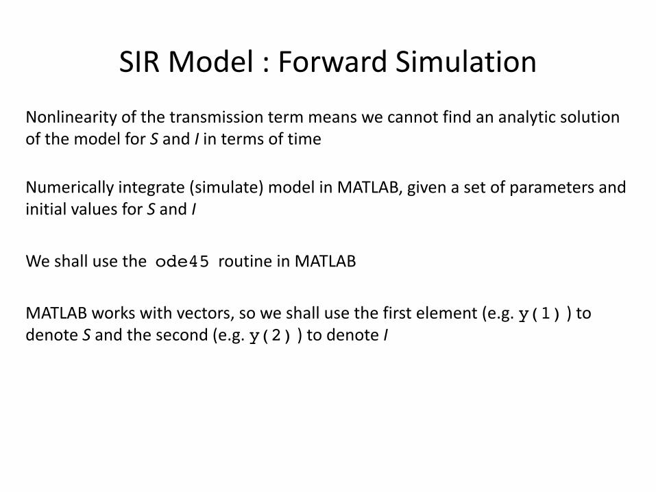
SIR Model : Forward SimulationNonlinearity of the transmission term means we cannot find an analytic solution of the model for S and I in terms of time
Numerically integrate (simulate) model in MATLAB, given a set of parameters and initial values for S and I
We shall use the ode45 routine in MATLAB
MATLAB works with vectors, so we shall use the first element (e.g. y(1) ) to denote S and the second (e.g. y(2) ) to denote I
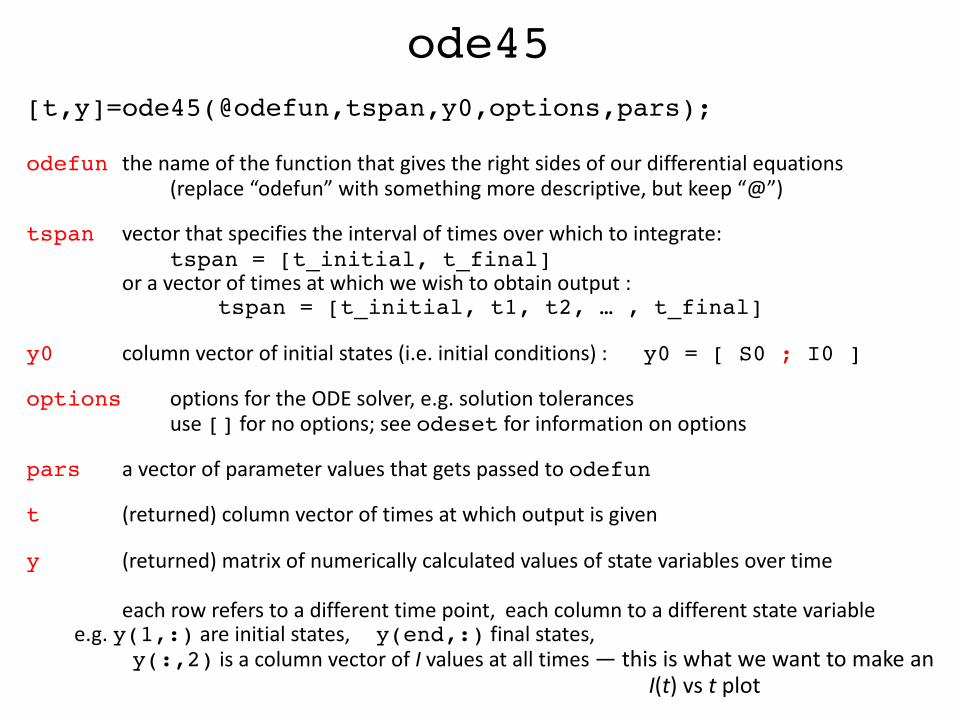
ode45[t,y]=ode45(@odefun,tspan,y0,options,pars);
odefun the name of the function that gives the right sides of our differential equations (replace “odefun” with something more descriptive, but keep “@”)
tspan vector that specifies the interval of times over which to integrate: tspan = [t_initial, t_final]
or a vector of times at which we wish to obtain output : tspan = [t_initial, t1, t2, … , t_final]
y0 column vector of initial states (i.e. initial conditions) : y0 = [ S0 ; I0 ]
options options for the ODE solver, e.g. solution tolerancesuse [] for no options; see odeset for information on options
pars a vector of parameter values that gets passed to odefun
t (returned) column vector of times at which output is given
y (returned) matrix of numerically calculated values of state variables over time
each row refers to a different time point, each column to a different state variable e.g. y(1,:) are initial states, y(end,:) final states,
y(:,2) is a column vector of I values at all times — this is what we want to make an I(t) vs t plot
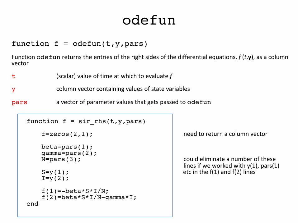
odefunfunction f = odefun(t,y,pars)Function odefun returns the entries of the right sides of the differential equations, f (t,y), as a column vector
t (scalar) value of time at which to evaluate f
y column vector containing values of state variables
pars a vector of parameter values that gets passed to odefun
function f = sir_rhs(t,y,pars)
f=zeros(2,1); need to return a column vector
beta=pars(1);gamma=pars(2);N=pars(3); could eliminate a number of these
lines if we worked with y(1), pars(1)S=y(1); etc in the f(1) and f(2) linesI=y(2);
f(1)=-beta*S*I/N;f(2)=beta*S*I/N-gamma*I;
end
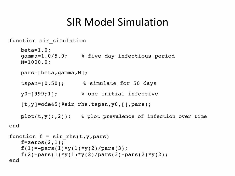
SIR Model Simulationfunction sir_simulation
beta=1.0;gamma=1.0/5.0; % five day infectious periodN=1000.0;
pars=[beta,gamma,N];
tspan=[0,50]; % simulate for 50 days
y0=[999;1]; % one initial infective
[t,y]=ode45(@sir_rhs,tspan,y0,[],pars);
plot(t,y(:,2)); % plot prevalence of infection over timeend
function f = sir_rhs(t,y,pars)f=zeros(2,1); f(1)=-pars(1)*y(1)*y(2)/pars(3);f(2)=pars(1)*y(1)*y(2)/pars(3)-pars(2)*y(2);
end
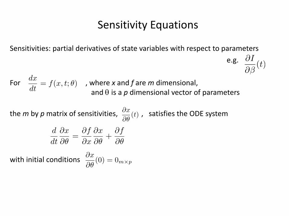
Sensitivity Equations
Sensitivities: partial derivatives of state variables with respect to parameterse.g.
For , where x and f are m dimensional,and q is a p dimensional vector of parameters
the m by p matrix of sensitivities, , satisfies the ODE system
with initial conditions
@I
@�(t)
dx
dt= f(x, t; ✓)
@x
@✓(t)
@x
@✓(0) = 0m⇥p
d
dt
@x
@✓=
@f
@x
@x
@✓+
@f
@✓
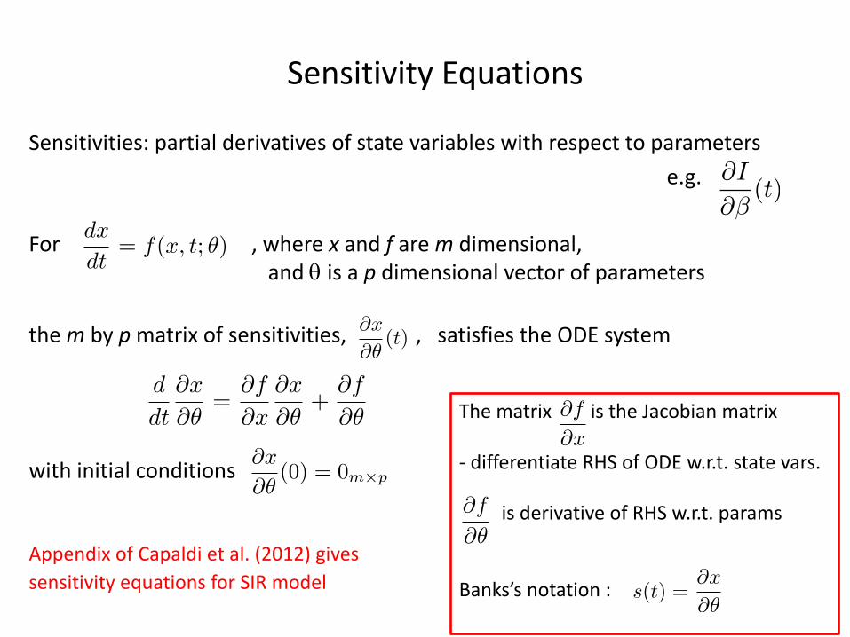
Sensitivity Equations
Sensitivities: partial derivatives of state variables with respect to parameterse.g.
For , where x and f are m dimensional,and q is a p dimensional vector of parameters
the m by p matrix of sensitivities, , satisfies the ODE system
with initial conditions
Appendix of Capaldi et al. (2012) gives sensitivity equations for SIR model
@I
@�(t)
dx
dt= f(x, t; ✓)
@x
@✓(t)
@x
@✓(0) = 0m⇥p
The matrix is the Jacobian matrix
- differentiate RHS of ODE w.r.t. state vars.
is derivative of RHS w.r.t. params
Banks’s notation :
@f
@x
@f
@✓
d
dt
@x
@✓=
@f
@x
@x
@✓+
@f
@✓
s(t) =@x
@✓
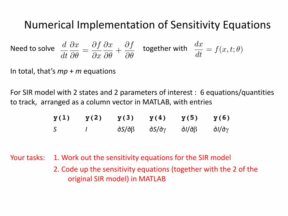
Numerical Implementation of Sensitivity Equations
Need to solve together with
In total, that’s mp + m equations
For SIR model with 2 states and 2 parameters of interest : 6 equations/quantities to track, arranged as a column vector in MATLAB, with entries
Your tasks: 1. Work out the sensitivity equations for the SIR model2. Code up the sensitivity equations (together with the 2 of the
original SIR model) in MATLAB
dx
dt= f(x, t; ✓)
d
dt
@x
@✓=
@f
@x
@x
@✓+
@f
@✓
y(1) y(2) y(3) y(4) y(5) y(6)S I ∂S/∂b ∂S/∂g ∂I/∂b ∂I/∂g

Behavior of the Sensitivity Equations?
Once you have the sensitivity equations running…
Plot curves of ∂I/∂b and ∂I/∂g on the same graph
Compare their shapes in the following situations:
1. R0 just above one, e.g. R0 = 1.2 (take b=0.24, g=0.2, integrate for 300 time units)
2. Intermediate R0 , e.g. R0 = 5 (take b=1, g=0.2, integrate for 50 time units)
3. Large R0 , e.g. R0 = 12 (take b=2.4, g=0.2, integrate for 50 time units)
Does the plot in case (1) say something interesting about our ability to separately estimate b and g?
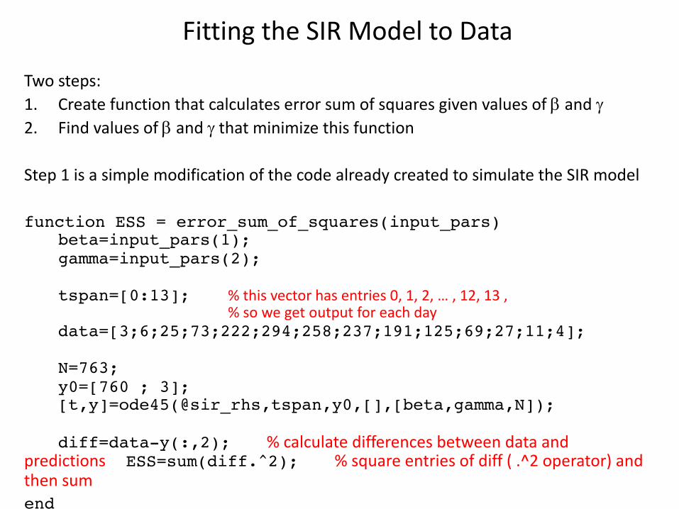
Fitting the SIR Model to Data
Two steps:1. Create function that calculates error sum of squares given values of b and g2. Find values of b and g that minimize this function
Step 1 is a simple modification of the code already created to simulate the SIR model
function ESS = error_sum_of_squares(input_pars)beta=input_pars(1);gamma=input_pars(2);
tspan=[0:13]; % this vector has entries 0, 1, 2, … , 12, 13 , % so we get output for each day
data=[3;6;25;73;222;294;258;237;191;125;69;27;11;4];
N=763;y0=[760 ; 3];[t,y]=ode45(@sir_rhs,tspan,y0,[],[beta,gamma,N]);
diff=data-y(:,2); % calculate differences between data and predictions ESS=sum(diff.^2); % square entries of diff ( .^2 operator) and then sumend

Fitting the SIR Model to Data
What does the error sum of squares function look like?Because it’s a function of two variables, it’s relatively easy to visualize, e.g. using a 3D plot or a contour plotMight be interesting to look at this before doing minimization…
beta_range=[1:0.05:3];gamma_range=[0.15:0.025:1];
% set up grid of values[GAMMA,BETA]=meshgrid(gamma_range,beta_range);
% calculate error sum of squares for each point on gridfor i=1:numel(beta_range)
for j=1:numel(gamma_range)ESS(i,j)=error_sum_of_squares([BETA(i,j),GAMMA(i,j)]);
endend
% do contour plot, with gamma on horizontal, beta on verticalfigure(1)contour(GAMMA,BETA,ESS,20)

Fitting the SIR Model to Data
What does the error sum of squares function look like?
Because it’s a function of two variables, it’s relatively easy to visualize, e.g. using a 3D plot or a contour plot
Might be interesting to look at this before doing minimization…
b on vertical axis
g on horizontal

Minimizing a Function: fminsearch
Optimization is a big area, with lots of different methods that could be used
We shall use MATLAB’s fminsearch , which implements the Nelder-Mead direct search simplex algorithm (Nelder & Mead, 1965; see also Walters et al. 1991, Lagarias et al. 1998)
Worth keeping in mind the difficulties (i.e. things that can and do go wrong) with minimization, particularly the possibility that a function has multiple local minima
(Our error sum of squares function looks nice, so we wade in without worrying too much…)
Minimizing a Function: fminsearch
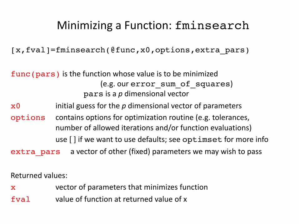
[x,fval]=fminsearch(@func,x0,options,extra_pars)
func(pars) is the function whose value is to be minimized (e.g. our error_sum_of_squares)
pars is a p dimensional vector x0 initial guess for the p dimensional vector of parametersoptions contains options for optimization routine (e.g. tolerances,
number of allowed iterations and/or function evaluations)use [ ] if we want to use defaults; see optimset for more info
extra_pars a vector of other (fixed) parameters we may wish to pass
Returned values:x vector of parameters that minimizes functionfval value of function at returned value of x

Example of use of fminsearchfunction test_minimization
x0=[1,4];[x,fval]=fminsearch(@simple_function,x0)
% as I don’t want to specify options or extra parameters% we can skip those arguments
end
function f = simple_function(pars)a=pars(1);b=pars(2);f= 2*(a-2)^2+3*(b-3)^2;
% embarrassingly simple function, whose minimum is at (2,3)end

Task: Fit SIR Model to Data
Use fminsearch on your error_sum_of_squares function to find the best-fitting values of b and g and the error sum of squares
Hint for initial guess at parameters: average duration of influenza infection is about 4 days, and R0 might be in the ballpark of 8
alternatively: did you get any idea from the contour plot?
[theta_hat,ess]=fminsearch(@error_sum_of_squares,[1,0.2])
Plot data and best fitting curve on the same graph
What is our best guess at the value of R0?
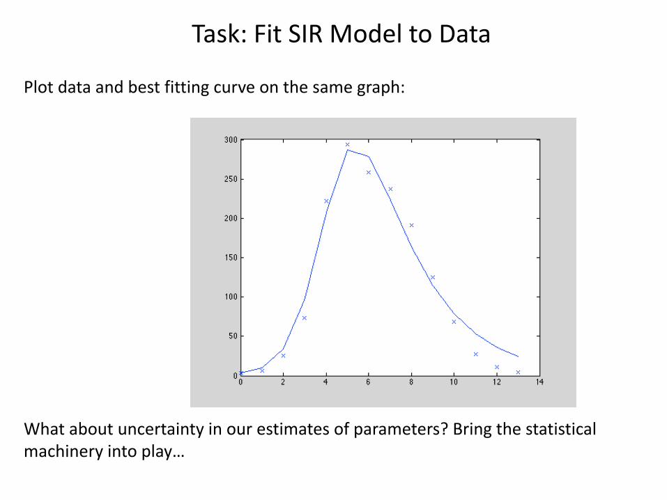
Task: Fit SIR Model to Data
Plot data and best fitting curve on the same graph:
What about uncertainty in our estimates of parameters? Bring the statistical machinery into play…
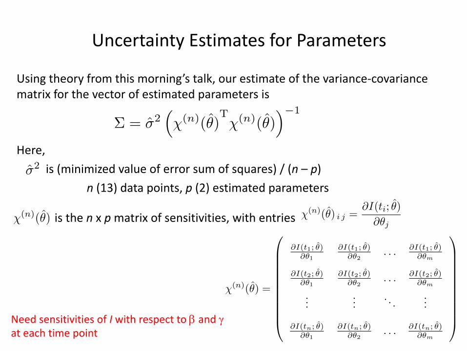
Uncertainty Estimates for Parameters
Using theory from this morning’s talk, our estimate of the variance-covariance matrix for the vector of estimated parameters is
Here,is (minimized value of error sum of squares) / (n – p)
n (13) data points, p (2) estimated parameters
is the n x p matrix of sensitivities, with entries
⌃ = �2⇣�(n)(✓)
T�(n)(✓)
⌘�1
�2
�(n)(✓) �(n)(✓) i j =@I(ti; ✓)
@✓j
�(n)(✓) =
0
BBBBBBBBBB@
@I(t1; ✓)@✓1
@I(t1; ✓)@✓2
. . . @I(t1; ✓)@✓m
@I(t2; ✓)@✓1
@I(t2; ✓)@✓2
. . . @I(t2; ✓)@✓m
......
. . ....
@I(tn; ✓)@✓1
@I(tn; ✓)@✓2
. . . @I(tn; ✓)@✓m
1
CCCCCCCCCCANeed sensitivities of I with respect to b and gat each time point
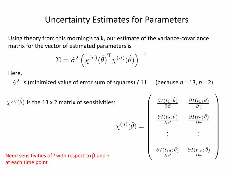
Uncertainty Estimates for Parameters
Using theory from this morning’s talk, our estimate of the variance-covariance matrix for the vector of estimated parameters is
Here,
is (minimized value of error sum of squares) / 11 (because n = 13, p = 2)
is the 13 x 2 matrix of sensitivities:
⌃ = �2⇣�(n)(✓)
T�(n)(✓)
⌘�1
�2
�(n)(✓)
Need sensitivities of I with respect to b and gat each time point
�(n)(✓) =
0
BBBBBBBBBB@
@I(t1; ✓)@�
@I(t1; ✓)@�
@I(t2; ✓)@�
@I(t2; ✓)@�
......
@I(t13; ✓)@�
@I(t13; ✓)@�
1
CCCCCCCCCCA
Uncertainty Estimates for Parameters
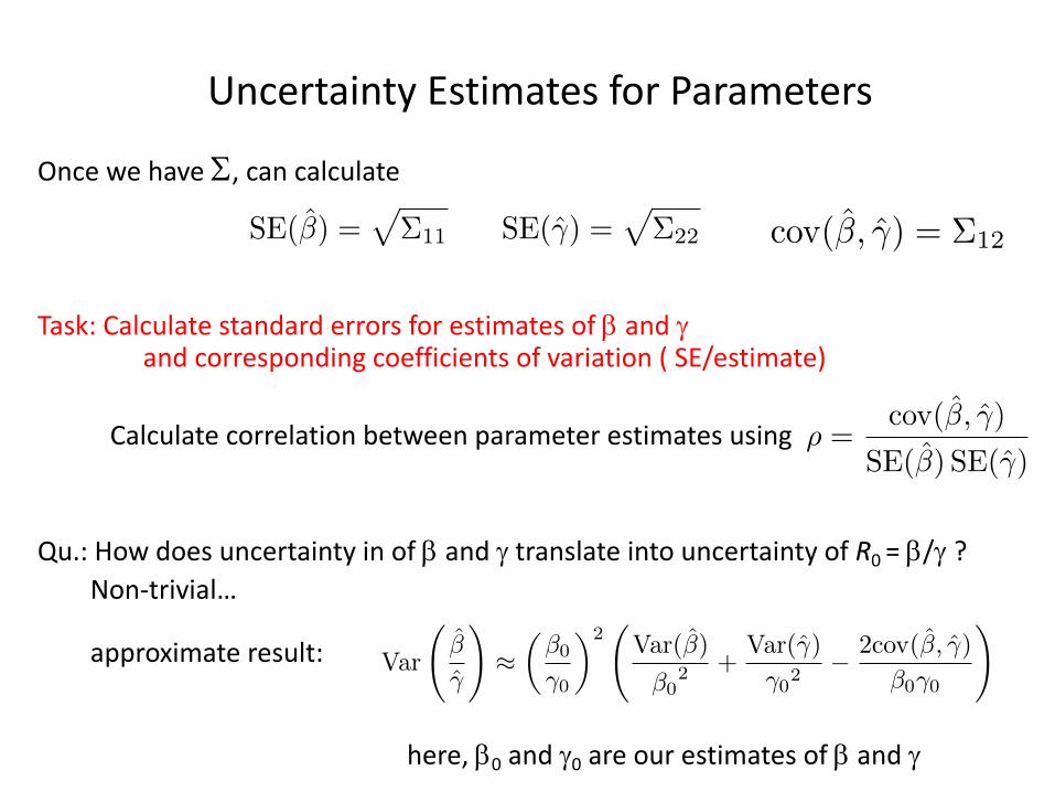
Once we have S, can calculate
Task: Calculate standard errors for estimates of b and gand corresponding coefficients of variation ( SE/estimate)
Calculate correlation between parameter estimates using
Qu.: How does uncertainty in of b and g translate into uncertainty of R0 = b/g ?Non-trivial…
approximate result:
here, b0 and g0 are our estimates of b and g
⇢ =cov(�, �)
SE(�) SE(�)
ESTIMATION & UNCERTAINTY QUANTIFICATION 559
Standard errors for the components of the estimator ✓LS are approximated bytaking square roots of the diagonal entries of ⌃, while the o↵-diagonal entries pro-vide approximations for the covariances between pairs of these components. Theuncertainty of an estimate of an individual parameter is conveniently discussed interms of the coe�cient of variation (CV), that is the standard error of an estimatedivided by the estimate itself. The dimensionless property of the CV allows foreasier comparison between uncertainties of di↵erent parameters. In a related fash-ion, the covariances can be conveniently normalized to give correlation coe�cients,defined by
⇢✓i,✓j =cov(✓i, ✓j)q
Var(✓i)Var(✓j). (16)
The asymptotic statistical theory provides uncertainties for individual parame-ters, but not for compound quantities—such as the basic reproductive number—thatare often of interest. For instance, if we had the estimator ✓LS = (�, �)T , a simplepoint estimate for R0 would be �/�, where � and � are the realized values of �and �. To understand the properties of the corresponding estimator we examinethe expected value and variance of the estimator �/�. Because this quantity is theratio of two random variables, there is no simple exact form for its expected valueor variance in terms of the expected values and variances of the estimators � and�. Instead, we have to use approximation formulas derived using the method ofstatistical di↵erentials (e↵ectively a second order Taylor series expansion, see [29]),and obtain
E
�
�
!⇡ �0
�0
1� cov(�, �)
�0�0+
Var(�)
�20
!, (17)
and
Var
�
�
!⇡✓�0
�0
◆2 Var(�)
�02 +
Var(�)
�02� 2cov(�, �)
�0�0
!. (18)
Here we have made use of the fact that E(�) = �0, the true value of the parameter,and E(�) = �0.
The variance equation has previously been used in an epidemiological settingby Chowell et al [13]. Equation (17), however, shows us that estimation of R0 bydividing point estimates of � and � provides a biased estimate of R0. The bias factorcan be written in terms of the correlation coe�cient and coe�cients of variationgiving
1� cov(�, �)
�0�0+
Var(�)
�20
!=⇣1� ⇢�,�CV�CV� + CV 2
�
⌘. (19)
This factor only becomes important when the CVs are on the order of one. In sucha case, however, the estimability of the parameters is already in question. Thus,under most useful circumstances, estimating R0 by the ratio of point estimates of� and � su�ces.
4. Generation of synthetic data, model fitting and estimation. In order tofacilitate our exploration of the parameter estimation problem, we choose to usesimulated data. This ‘data’ is generated using a known model, a known parameterset and a known noise structure, putting us in an idealized situation in which weknow that we are fitting the correct epidemiological model to the data, that thecorrect statistical model is being employed and where we can compare the estimated
cov(�, �) = ⌃12SE(�) =p⌃11 SE(�) =
p⌃22
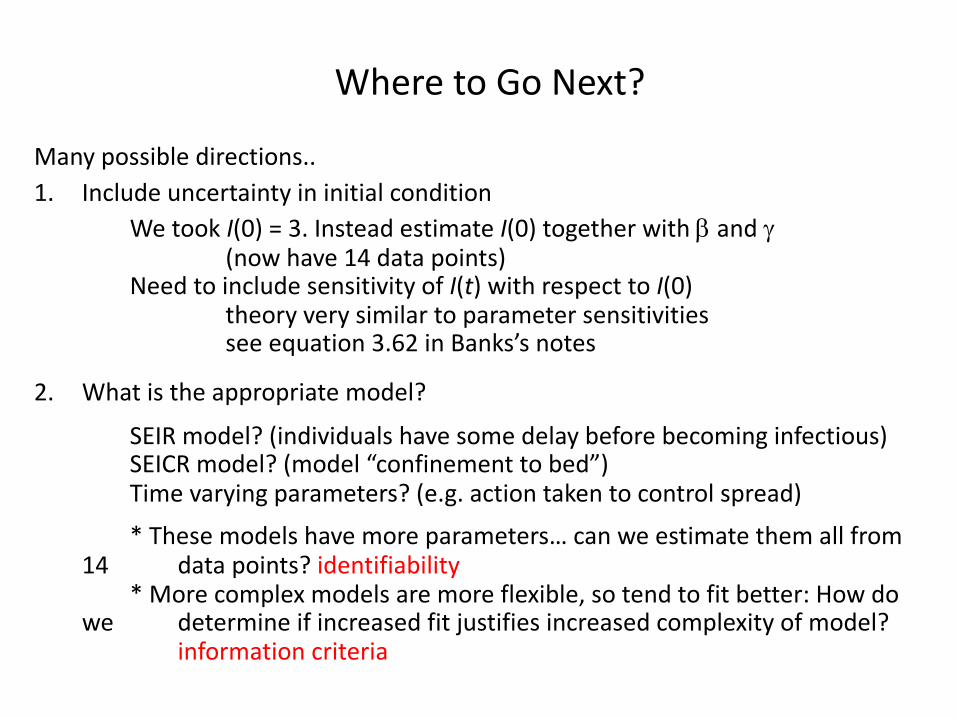
Where to Go Next?
Many possible directions..1. Include uncertainty in initial condition
We took I(0) = 3. Instead estimate I(0) together with b and g(now have 14 data points)
Need to include sensitivity of I(t) with respect to I(0)theory very similar to parameter sensitivitiessee equation 3.62 in Banks’s notes
2. What is the appropriate model?
SEIR model? (individuals have some delay before becoming infectious)SEICR model? (model “confinement to bed”)Time varying parameters? (e.g. action taken to control spread)* These models have more parameters… can we estimate them all from
14 data points? identifiability* More complex models are more flexible, so tend to fit better: How do
we determine if increased fit justifies increased complexity of model?information criteria
References
Anonymous (1978). Influenza in a boarding school. Brit. Med. J. 6112, 587.
Banks, H.T., et al. (2014). Modeling and Inverse Problems in the Presence of Uncertainty. CRC Press.
Capaldi, A., et al. (2012). Parameter estimation and uncertainty quantification for an epidemic model. Math. Biosci. Eng. 9, 553-576.
Lagarias, J.C., et al. (1998). Convergence properties of the Nelder-Mead simplex method in low dimensions. SIAM J. Optim. 9, 112-147.
Nelder, J.A. & Mead, R. (1965). A simplex method for function minimization. Comp. J. 7, 308-313.
Walters, F.H., et al. (1998). Sequential Simplex Optimization. CRC Press