Embed Size (px)
Citation preview
Sensing and Measurement for Advanced Power Grids
Jeffrey D. Taft, PhD
Distinguished Engineer Cisco Systems
Paul De Martini
Visiting Scholar Caltech Resnick Institute
Version 1.3
October 22, 2012
Abstract
Data acquisition for large scale, physically distributed system such as power grids is facing a transformation as the number of end points providing data increases due to new functionality associated with grid modernization. Consequently, traditional techniques are facing challenges that are structural in nature, meaning the centralized hub and spoke model for SCADA is becoming inadequate for future large scale systems. These challenges may be addressed with distributed intelligence architectures, but to do so requires an understanding of sensing and measurement principles that apply to the class of systems represented by electric grids and other structured dynamic environments.
These principles include the extension of system state and observability to large scale physically distributed systems, which means that these concepts must be integrated with communication networking. Consequently, the measurement system designer must also understand how appropriate sensor network architecture principles apply to the distributed system data acquisition problem.
This paper describes the principles system state and observability as applied to power grids, as well as observability strategy and sensor allocation guidelines.

Introduction and Background
Utility measurement and control systems and data processing systems have largely been centralized in nature. Grid control systems typically reside in control or operations centers and rely upon what have generally been low complexity communications to field devices and systems. There are a few distributed control systems for utility applications, including a wireless mesh system for performing fault isolation using peer-to-peer communications among devices on feeder circuits outside of the substations. In addition, certain protection schemes involve substation-to-substation communication and local processing. In general however, centralized systems are the rule for electric grids. Both utilities and makers of various grid control systems have recognized the value of distributed intelligence, especially at the distribution level. We define distributed intelligence as the embedding of digital processing and communications in a physically dispersed, multi-element environment (specifically the power grid infrastructure but physical networks in general). In the area of sensing, measurement and data acquisition, key issues are:
• Observability and system state – key concepts that can be used to guide the design of sensor systems for physical systems with topological structure and system dynamics
• Sensing and measurement – determination of quantities to be sensed, type and location of sensors, and resulting signal characteristics
• Data acquisition – collection of sensor data, sensor data transport
• Sensor network architecture – elements, structure, and external properties of sensor networks
• Communications for sensor networks
These considerations and the increasing complexity of modern power grids lead to the conclusion that the electric utility engaged in grid modernization must consider creating an observability strategy to guide the implementation of sensing for modern grid operation. Such a strategy must, as always, draw upon the detailed knowledge of the system in question on the part of the engineers who know it best. But it must also apply tools and concepts drawn from control theory, communication networking, sensor networking, optimization, and recent developments in sensing for power grids to develop a systematic approach to providing the needed measurements in a cost-effective and manageable way. Ultimately, this is a technical tool to help address risk associated with investment in sensing and measurement as part of the grid control architecture.
This paper addresses key issues in building an observability strategy for power grids by introducing the appropriate concepts and tools and by providing experience-based guidelines and design principles of practical value.
Terminology
Before delving into sensor issues, we define some basic terminology in Table 1 below.
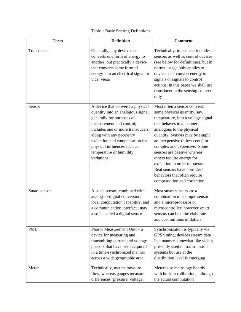
Table 1 Basic Sensing Definitions
Term Definition Comment
Transducer Generally, any device that converts one form of energy to another, but practically a device that converts some form of energy into an electrical signal or vice versa
Technically, transducer includes sensors as well as control devices (see below for definitions), but in normal usage only applies to devices that convert energy to signals or signals to control actions; in this paper we shall use transducer in the sensing context only
Sensor A device that converts a physical quantity into an analogous signal, generally for purposes of measurement and control; includes one or more transducers along with any necessary excitation and compensation for physical influences such as temperature or humidity variations.
Most often a sensor converts some physical quantity, say, temperature, into a voltage signal that behaves in a manner analogous to the physical quantity. Sensors may be simple an inexpensive (a few cents) or complex and expensive. Some sensors are passive whereas others require energy for excitation in order to operate. Real sensors have non-ideal behaviors that often require compensation and correction.
Smart sensor A basic sensor, combined with analog-to-digital conversion, local computation capability, and a communication interface; may also be called a digital sensor
Most smart sensors are a combination of a simple sensor and a microprocessor or microcontroller; however smart sensors can be quite elaborate and cost millions of dollars.
PMU Phasor Measurement Unit – a device for measuring and transmitting current and voltage phasors that have been acquired in a time-synchronized manner across a wide geographic area
Synchronization is typically via GPS timing; devices stream data in a manner somewhat like video; presently used on transmission systems but use at the distribution level is emerging
Meter Technically, meters measure flow, whereas gauges measure differences (pressure, voltage,
Meters use metrology boards with built-in calibration, although the actual computation
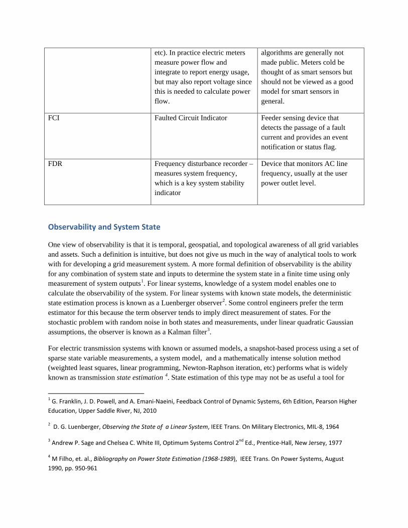
etc). In practice electric meters measure power flow and integrate to report energy usage, but may also report voltage since this is needed to calculate power flow.
algorithms are generally not made public. Meters cold be thought of as smart sensors but should not be viewed as a good model for smart sensors in general.
FCI Faulted Circuit Indicator Feeder sensing device that detects the passage of a fault current and provides an event notification or status flag.
FDR Frequency disturbance recorder – measures system frequency, which is a key system stability indicator
Device that monitors AC line frequency, usually at the user power outlet level.
Observability and System State
One view of observability is that it is temporal, geospatial, and topological awareness of all grid variables and assets. Such a definition is intuitive, but does not give us much in the way of analytical tools to work with for developing a grid measurement system. A more formal definition of observability is the ability for any combination of system state and inputs to determine the system state in a finite time using only measurement of system outputs1. For linear systems, knowledge of a system model enables one to calculate the observability of the system. For linear systems with known state models, the deterministic state estimation process is known as a Luenberger observer2. Some control engineers prefer the term estimator for this because the term observer tends to imply direct measurement of states. For the stochastic problem with random noise in both states and measurements, under linear quadratic Gaussian assumptions, the observer is known as a Kalman filter3.
For electric transmission systems with known or assumed models, a snapshot-based process using a set of sparse state variable measurements, a system model, and a mathematically intense solution method (weighted least squares, linear programming, Newton-Raphson iteration, etc) performs what is widely known as transmission state estimation 4. State estimation of this type may not be as useful a tool for
1 G. Franklin, J. D. Powell, and A. Emani-Naeini, Feedback Control of Dynamic Systems, 6th Edition, Pearson Higher Education, Upper Saddle River, NJ, 2010
2 D. G. Luenberger, Observing the State of a Linear System, IEEE Trans. On Military Electronics, MIL-8, 1964
3 Andrew P. Sage and Chelsea C. White III, Optimum Systems Control 2nd Ed., Prentice-Hall, New Jersey, 1977
4 M Filho, et. al., Bibliography on Power State Estimation (1968-1989), IEEE Trans. On Power Systems, August 1990, pp. 950-961
distribution grids, due to their topological complexities and the fact that they are generally unbalanced. We rely more on state measurement and less on state estimation in the distribution case whenever we can arrange for the necessary instrumentation. The need to provide grid state for control purposes leads to the need for observability and therefore sensing and measurement.
We consider the definition of state in order to define observability for power grids. State is the minimum set of values (state variables) that describe the instantaneous condition of a dynamic system. State variables may be continuous (physical systems), discrete (logical systems and processes), or stochastic (such as Markov model states). For many types of systems and for linear systems in particular, the mathematics of state are well defined in the context of differential equation solutions of system dynamics. State has the property that future state of a dynamic system is completely defined by the present state and system inputs only. Knowledge of past state trajectory or past inputs is not necessary. Mathematically, we describe state for dynamic systems as:
dx/dt = F[x(t),u(t)]
for continuous time systems and :
x(k+1) = A[x(k),u(k)]
for discrete time systems, where F and A represent system dynamics models, x is system state and u is the system input5.
For stochastic variables we may employ the concept of stochastic state as embodied in (possibly hidden) Markov models, where the observed statistical behavior relates to an underlying stochastic state model6. A Markov model is a state model where transitions from state to state are described by probabilities rather than deterministic dynamics. A matrix of transition probabilities plays the part of the state transition matrix for deterministic systems. The Markov model concept is a useful mechanism to enable us to include power quality as an element of grid state.
The concept of state applies equally well for logical systems with discrete states. The open/closed or on/off states of switches are prime examples and state transition diagrams and matrices are used to describe discrete system behavior. Logical systems are often described by state transition diagrams but these can be converted to discrete state transition tables7, analogous to the state transition matrices F and A in the linear versions of equations above.
For power grid observability, we find it useful to use an extended distribution grid state definition, where we augment the VIPQ (voltage, current, real power, reactive power) view of grid power state with
5 Paul M. DeRusso Rob J. Roy and Charles M. Close, State Variables for Engineers, John Wiley and Sons, New York, 1965
6 Jia Li, Hidden Markov Model, The Pennsylvania State University, available online: tat.psu.edu/~jiali/course/stat597e/notes2/hmm.pdf
7 Frederick J. Hill and Gerald R. Peterson, Switching Theory and Logical Design, 2nd Edition, John Wiley and Sons, New York, 1974
additional elements, such circuit parameters, storage charge state, Demand Response Available Capacity (DRAC) and technical losses. We can calculate circuit section impedance values from online measurements during the grid state determination process. When grid state is fully determined, we may then use it to define other grid conditions of interest. Outage, for example, which is the loss of voltage at energy delivery nodes on the grid, can be seen as a situation where certain grid state variables, namely node voltages, are at or near zero. We can then determine the outage state by reference to grid electrical state variables.
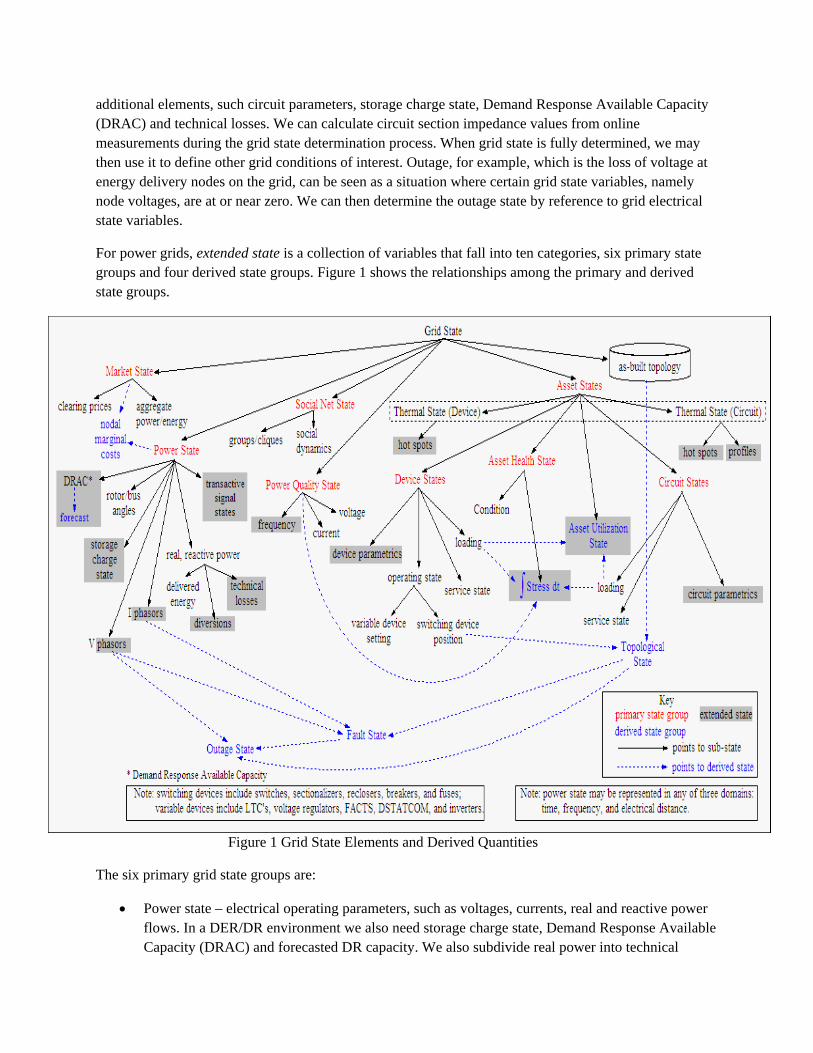
For power grids, extended state is a collection of variables that fall into ten categories, six primary state groups and four derived state groups. Figure 1 shows the relationships among the primary and derived state groups.
Figure 1 Grid State Elements and Derived Quantities
The six primary grid state groups are:
• Power state – electrical operating parameters, such as voltages, currents, real and reactive power flows. In a DER/DR environment we also need storage charge state, Demand Response Available Capacity (DRAC) and forecasted DR capacity. We also subdivide real power into technical
losses, delivered energy (delivered real power integrated over time), and diversions. Normally, we use RMS values for voltage and current, but in more advanced observability solutions we extend these to actual phasors. We include Locational Marginal Pricing (LMP), Distribution-LMP (D-LMP), and transactive signal states (as they experience disaggregation or diffusion) as elements of power state.
• Power quality state – power quality measurements are the manifestation of underlying quality state, which we consider as a hidden Markov process. Quality issues manifest themselves in deviations of the voltage and current waveforms from sinusoids of fixed frequency. For voltage, amplitude variations are essential, whereas harmonic distortion applies to both voltage and current.
• Thermal state – thermal state is reflected in temperatures, for which we keep two types: hotspots (for both devices and circuits) and temperature profiles or distributions (for circuits). Temperature can be measured directly in many cases, although with some devices, actual hotspots may be internal and not easily accessible to instrumentation). Devices also have temperature distributions, but we normally are interested only in their hotspot temperatures.
• Device State – consists of service state (in service, out of service, failed), setting or position, loadings, and device parametrics (impedance, dynamic rating). Settings apply to devices that have multiple positions or continuous adjustability, such as load tap changers, voltage regulators, static VAr compensators, etc. Device positions apply to binary devices such as switches, reclosers, fuses, and breakers.
• Circuit State – consists of service state (in or out of service, failed), loading, and parametrics (circuit segment impedance, dynamic rating). Circuit impedances are distributed parameters, but for the purposes of smart grid applications may be lumped on a per segment basis.
• Asset Health State –consists of two element sets: condition (present health state) of devices and circuits, and accumulated stress. Stress is manifested differently for different devices and for circuits, but the stressors result in accumulation of stress in forms that accelerate failure and degrade performance and can be treated through component loss of life and estimated time to failure.
• Market State – increasingly important as markets become elements of grid control loops for such things as Demand Response and Distributed Energy Resource integration
• Social Network State – as loads become transactive, as local area grids and microgrids develop, and as markets are opened to smaller users, the social interaction aspects of grid operation are beginning to evolve; consequently understanding social network state as it impacts grid management is just beginning to be recognized for its importance
The four derived state groups are:
• Outage State – list of all service delivery endpoints that have lost voltage; outage state is a discrete logical process, as is fault state
• Fault State – list of all devices and circuits that have shorted or open circuit faults, fault locations (for circuits), fault type
• Asset Utilization State – power loading vs. ratings, and load balance of devices and circuits; duty cycles, operation count rates.
• Topological state –in general, distribution grid connectivity may be complex due to sectionalization and the interconnection of circuits through inter-tie switches. As-built topology is quasi-static and comes from design data and field as-built data using default switch positions. Real time as-operated topology derives from the as-built topology and the actual grid switch positions. Thus topological state is derived from the grid components but is a property of the system as a whole. We therefore treat as-operated topology as a derived system state element (derived from as-built topology and switch settings).
Since knowledge of grid state is fundamental to most grid control and management applications, determination of state is vital. This leads us to focus on grid state determination.
We use the term grid state determination for the process involved on a power grid, since we may measure grid power states directly, or we may make measurements from which state elements can be calculated or estimated, or we may use a mix of measured and estimated states In the case of power grids, we want to know the grid state on a moment to moment basis, since this information is the foundation of many smart grid functions and capabilities. Determining extended grid state is a multi-stage process, comprising:
• Sensing, measurement and data acquisition – the basic processes of obtaining raw grid data, with conversion from analog to digital form
• Filtering, linearization, scaling, and units conversion – conversion and processing of raw digital data from uncompensated integer counts to compensated, linearized values, scaled to engineering or physical quantity units as opposed to dimensionless integers
• Representation – conversion of physical variables into forms suitable for analysis and use in control in any of several domains: time, frequency, geospatial, or electrical distance from a reference points such as a substation
• State formation – construction of actual grid state elements; may involve several computational processes such as extraction of parameters from data sets, estimation where necessary, and then assembly and aggregation of grid state elements
• Distribution and persistence – grid state elements must be made available to various decision and control processes, and may have to be persisted in any of several tiers of data storage, depending on the various uses for the data
Aggregation may occur at several levels. Raw instantaneous voltage or current samples may be aggregated into records so that they can be processed into Root-Mean-Square (RMS) values and also analyzed for harmonic content. At another scale, we may aggregate voltage samples taken at various points in a meter network into a voltage profile as a function of electrical distance for a feeder. If we have meters that can measure real and reactive power, we can aggregate values to determine power flows at
various points on a feeder and may do likewise with DRAC values. We may aggregate current and power flows from points to feeder segments to feeder sections to substations to transmission lines to service areas to control areas.
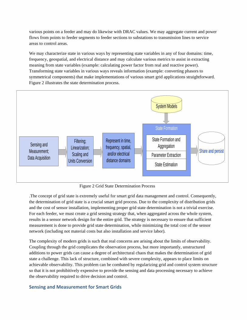
We may characterize state in various ways by representing state variables in any of four domains: time, frequency, geospatial, and electrical distance and may calculate various metrics to assist in extracting meaning from state variables (example: calculating power factor from real and reactive power). Transforming state variables in various ways reveals information (example: converting phasors to symmetrical components) that make implementations of various smart grid applications straightforward. Figure 2 illustrates the state determination process.
State Formation
Sensing and Measurement;
Data Acquisition
Filtering;Linearization;Scaling and
Units ConversionParameter Extraction
State Formation and Aggregation
System Models
Represent in time, frequency, spatial, and/or electrical
distance domains
Share and persist
State Estimation
Figure 2 Grid State Determination Process
.The concept of grid state is extremely useful for smart grid data management and control. Consequently, the determination of grid state is a crucial smart grid process. Due to the complexity of distribution grids and the cost of sensor installation, implementing proper grid state determination is not a trivial exercise. For each feeder, we must create a grid sensing strategy that, when aggregated across the whole system, results in a sensor network design for the entire grid. The strategy is necessary to ensure that sufficient measurement is done to provide grid state determination, while minimizing the total cost of the sensor network (including not material costs but also installation and service labor).
The complexity of modern grids is such that real concerns are arising about the limits of observability. Coupling through the grid complicates the observation process, but more importantly, unstructured additions to power grids can cause a degree of architectural chaos that makes the determination of grid state a challenge. This lack of structure, combined with severe complexity, appears to place limits on achievable observability. This problem can be combated by regularizing grid and control system structure so that it is not prohibitively expensive to provide the sensing and data processing necessary to achieve the observability required to drive decision and control.
Sensing and Measurement for Smart Grids
The design of a sensing network for a modern power grid should be viewed and formulated as an optimization problem. Fundamentally, we wish to minimize CapEx while managing (bounding) Opex over a time horizon and yet ensure that observability requirements are met. This can be formulated mathematically; the solution requires the use of sophisticated mathematical and software tools, such optimizations have been performed to determine best locations for reclosers to maximize reliability, and best locations for PMU’s on transmission systems, among other goals. Here we suggest a more practical route – the use of guidelines and design rules. Before introducing the set of guidelines for developing an observability strategy (which leads to a sensor network design), we must cover some additional material.
Keep in mind that there are actually four types of networks involved in the modern power grid: in addition to the electric grid, we have a communications network, a financial network, and a social network (actually potentially several social networks). In addition, the power grid is composed of the electric network, a sensor sub-network and a control sub-network. We must consider observability for the power grid, and for the financial and social networks; the communications grid and the control sub-network are not at issue. We begin with the power grid.
Power Grid Transducers and Smart Sensors
Power grids use a wide array of sensing devices, including sensing built into grid control devices, as well as explicit sensors. A key tradeoff for sensor network design has been the use of many low costs sensors (example: Faulted Circuit Indicators or FCI’s) vs. the use of a smaller number of high end sensors (example: multi-variable line sensors). The best example of a high end sensor is the phasor measurement units used on transmission systems to provide synchronized phasor measurement. As modern grid complexity increases, the move toward synchronized measurement necessitated by advanced control requirements tends toward the use of high end sensors, even to the point of using synchronized phasor measurement units (PMU’s) on distribution feeders. Despite this trend, it is still valid to consider the use of low end sensors and in the more sophisticated approaches, to employ a mix of sensor types. Part of the observability strategy issue is to determine the mix of sensors to be used for a particular system. Observability strategy is more of a problem for distribution grids than for transmission grids due to structural and emerging functional complexity differences. Smart line sensors and advanced meters are two logical options for distribution grid power state sensing.
Basic Smart Sensor Functionality
A smart sensor is one that contains a physical parameter transducer, means to convert analog sensor signals to digital form, a digital processor, with memory, embedded software, possibly downloaded applications, and digital communications capability. Present line sensors are usually implemented as a combination of a set of line transducers and an RTU with embedded processing capability, as well as one of more communication interfaces.
A typical configuration of a distribution power line electrical sensor would use three signal channels for phase voltage waveform measurement, three channels for phase current waveform measurement, one channel for neutral current measurement, and one channel for temperature measurement. Voltage and current waveforms should be sampled at 128 or more samples per cycle8. Signal channels must include 8 IEEE Std 1159-1995 IEEE Recommended Practice for Monitoring Electric Power Quality. Available online

analog anti-aliasing filters. Simultaneous sample/holds are preferred because some processing functions are concerned with relative phase. Raw sensors should be accurate to 0.5% of full scale and have analog bandwidths of at least 10 kHz.
The smart sensor platform must contain at least one digital processor with sufficient processing capacity and memory to support local data acquisition, digital signal processing, and digital communications. This platform must be capable of receiving downloaded applications and of performing bi-directional communications over various communication media and with various protocols. It must provide data security functions including:
• Encryption • Identification • Authentication • Non-repudiation • Tamper detection/prevention
The smart sensor should support IPv6-enabled digital communications. It should support standard protocols for network routing, timing (IEEE 15889), and management (SNMP10 for example).
It is useful for the sensors to support Transducer Electronic Data Sheets (TEDS11), to provide management of sensor –specific information so that multiple data collection engines or controls can access the sensor without need to access a central data collection system to obtain calibrated data.
Meters as Sensors
When a utility has or will be deploying an Advanced Meter Infrastructure (AMI) system, it is logical to consider how this meter system may be used as a grid sensor network. Many residential meters are capable of sensing and reporting secondary voltage in addition to usage data. Newer Commercial and Industrial (C&I) meters have significant capabilities for measuring and reporting real and reactive power, power factor, and harmonics in voltage and current.
When an AMI system is in place, careful selection of meters that are approximately evenly spaced along a distribution feeder (in terms of distribution transformer electrical distance from the substation) should enable the determination of feeder voltage profiles, which would be valuable in voltage regulation. In addition, instant voltage readings (“pings”) should enable rapid determination of outage extent and restoration progress. Rapid voltage reading could also enable operational verification for grid devices such as switched, reclosers, and capacitors, by providing voltage values just before and just after device
9 IEEE Standards Association, IEEE Std 1588 – Standard for a Precision Clock Synchronization Protocol for Networked Measurement and Control Systems, 2011, available online: http://standards.ieee.org/findstds/interps/1588-2008.html
10 Simple Network Management Protocol
11 NIST, IEEE P1451 Smart Transducer Interface Standard, see http://www.nist.gov/el/isd/ieee/ieee1451.cfm, and available online at http://www.ieee.org/index.html

command issuance. Those meters that can record voltage sags or compute harmonics in power waveforms could be used to measure power quality state elements. All of these functions have in fact been tried with AMI and C&I meter systems.
In practice, residential meter systems have not proven to be the all-encompassing sensor fabrics for power grids that many have desired them to be. There are several reasons for this:
• Residential meters are designed for lowest cost and so do not have advanced sensing capabilities; this means that they do not measure many of the useful quantities needed for grid state determination; in some cases, the existing measurement are not made in a useful manner
• Meter communication networks have often been designed only to support usage reporting and so do not have the bandwidth and latency capabilities to support operation as a grid sensor network; this means that the meters cannot provide sensor-type data fast enough to be useful for any but the slowest (read: old style) distribution automation control systems
• Meter communication protocols until recently did not support sensor-like operation, having been developed from a usage reporting point of view; consequently it is normally necessary to go through the meter data collection head end to obtain any meter data, including voltage readings; full IPv6 stacks in the meters can alleviate this
• Meter installation databases generally relate geospatial and customer information to the meter, but there is often no documented relationship to power grid connectivity; however power grid connectivity is the context in which sensed data must be interpreted
• Residential meter systems and their communication networks can take very long time periods to re-converge upon partial or complete power restoration, so the meters do not come online fast enough to report grid state information that would be useful for restoration operations or grid control during restoration
• Wireless mesh-based meter communications networks are “lossy”, meaning that they are unreliable in terms of message packet delivery which is not a severe problem for usage reporting, but is a severe problem for control system support
• Most residential meters do not have a strong notion of time, so that time-synchronized measurements, important for control system operation, are not possible with meters
For meters to be useful for any but the simplest distribution automation functions, these issues must be remedied. This means, reliable communications, efficient communication protocols and interfaces, IPv6 support, support for time synchronization via IEEE 1588 time service, synchronized sampling capability, and sensor-grade measurement functions for more than just usage.
Data Acquisition
Power grid devices and sensors operate in one or more of five data acquisition modes:
• Polling – a polling master queries the device, which response with the most recent values of the specified data points; polling is usually on a regular schedule and data size per query is modest
• Report by exception – the device pushes a data value to the master when the data changes by a specified amount
• Streaming – sensor sends a continuous stream of data, once streaming is initiated, until streaming is terminated by command or abnormal exit condition
• Interrogation of stored files – the device maintains a log or data file; upon query, it transmits the log or file to the master; differs from polling in terms of data size per query and frequency/regularity of the query
• Asynchronous event message – the device uses internal processing to detect a specific condition indicated by the data and spontaneously sends an event message to the master or any subscribing system- the message may or may not contain actual sensor data relevant to the event; the internal event can be a clock signal or countdown so that the messages are sent on a regular basis, but initiated by the sensor, not a central controller
Polling is common in grid control systems, but report by exception is used in some systems to reduce data volumes and therefore communication line bandwidth. Not all utilities are willing to use report by exception. Streaming is common for advanced sensors such as PMU-based wide area measurement systems (WAMS). Interrogation of stored data files is common for meters and for data loggers and grid devices that collect records on a power waveform-triggered basis. Asynchronous event messages are becoming more common in devices that contain significant local processing and are therefore able to detect and report events.
Collection of the data in large scale systems such as smart grids presents issues of cycle time, data bursting, and sample skew. In the typical round-robin scanning approach taken by many standard SCADA12 systems, the time skew between first and last samples represents an issue for control systems that is insignificant when the scan cycle time is short compared to system dynamics, but as dynamics in increase in bandwidth with advanced regulation and stabilization, and as the number of sensing points increases, the sample time skew problem becomes significant.
In a control system where distributed endpoints are free-running and each is updating its measurement(s) asynchronously, round robin collection of the data can result in time skew among samples. This can cause a degradation of accuracy in creating state estimates from the data samples, with resultant degradation of control performance
12 Supervisory Control and Data Acquisition
Final Control Element
ZOHControl Law
_
S/H
S
Sensor/Measurement
∆C
S/H Sensor/Measurement
S/H Sensor/Measurement
∆1
∆2
∆Ν
System Under Control
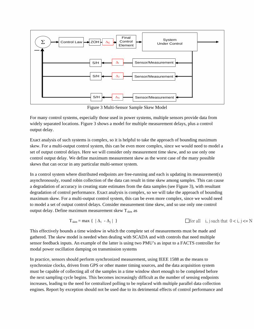
Figure 3 Multi-Sensor Sample Skew Model
For many control systems, especially those used in power systems, multiple sensors provide data from widely separated locations. Figure 3 shows a model for multiple measurement delays, plus a control output delay.
Exact analysis of such systems is complex, so it is helpful to take the approach of bounding maximum skew. For a multi-output control system, this can be even more complex, since we would need to model a set of output control delays. Here we will consider only measurement time skew, and so use only one control output delay. We define maximum measurement skew as the worst case of the many possible skews that can occur in any particular multi-sensor system.
In a control system where distributed endpoints are free-running and each is updating its measurement(s) asynchronously, round robin collection of the data can result in time skew among samples. This can cause a degradation of accuracy in creating state estimates from the data samples (see Figure 3), with resultant degradation of control performance. Exact analysis is complex, so we will take the approach of bounding maximum skew. For a multi-output control system, this can be even more complex, since we would need to model a set of output control delays. Consider measurement time skew, and so use only one control output delay. Define maximum measurement skew Tskm as
Tskm = max { | Δ i - Δ j | } for all i, j such that 0 < i, j <= N
This effectively bounds a time window in which the complete set of measurements must be made and gathered. The skew model is needed when dealing with SCADA and with controls that need multiple sensor feedback inputs. An example of the latter is using two PMU’s as input to a FACTS controller for modal power oscillation damping on transmission systems
In practice, sensors should perform synchronized measurement, using IEEE 1588 as the means to synchronize clocks, driven from GPS or other master timing sources, and the data acquisition system must be capable of collecting all of the samples in a time window short enough to be completed before the next sampling cycle begins. This becomes increasingly difficult as the number of sensing endpoints increases, leading to the need for centralized polling to be replaced with multiple parallel data collection engines. Report by exception should not be used due to its detrimental effects of control performance and

the communication network should be designed to handle the data volumes associated with the full sensor set. This leads to distributed data collection and to the use of advanced communication network protocols.
Distributed Data Acquisition
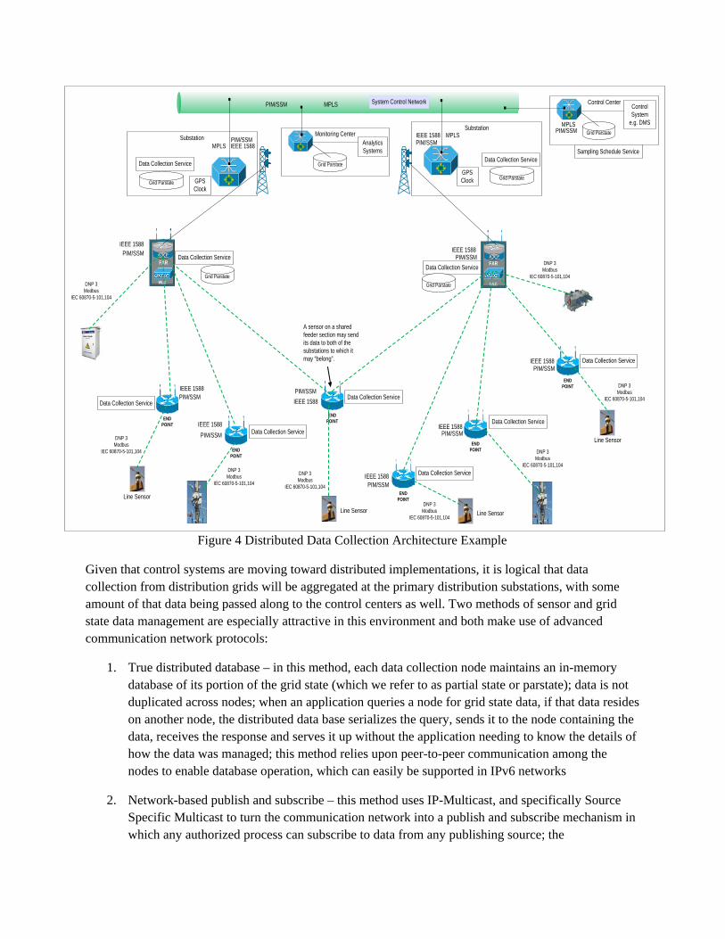
Distribution SCADA has traditionally been structured as a simple hub-and spoke centralized network. As more smart devices are deployed and as latency requirements move ever lower, the advantages of a distributed SCADA approach become evident. In such an approach, multiple data collection engines are deployed throughout the distribution grid. This is fundamentally different from the logical distributed data collection approach used by some Energy Management Systems (EMS – grid control systems) where multiple front end communication engines are located in a single control center. Such an approach is properly viewed as distributed, but has the disadvantage of still using a hub and spoke centralized network structure. In the geographically distributed approach, the data collection engines are moved out of the control center and into other places in the power system. These places can be the transmission and primary distribution substations, but we can go further and place smaller data collection engines at tactical locations on distribution feeders. In such an approach, there is more mesh-like peer-to-peer data flow, which can relieve the need to have a very large data pipe into the control center. Figure 4 illustrates such an approach.
SubstationSubstation
END POINT
END POINT
END POINT
FAR
WLC
FAR
WLC
END POINT
END POINT
END POINT
System Control Network
Data Collection Service
DNP 3Modbus
IEC 60870-5-101,104 DNP 3Modbus
IEC 60870-5-101,104DNP 3
ModbusIEC 60870-5-101,104
DNP 3Modbus
IEC 60870-5-101,104
DNP 3Modbus
IEC 60870-5-101,104
DNP 3Modbus
IEC 60870-5-101,104
DNP 3Modbus
IEC 60870-5-101,104
IEEE 1588IEEE 1588
IEEE 1588
IEEE 1588
IEEE 1588
IEEE 1588
IEEE 1588
IEEE 1588
PIM/SSM
PIM/SSMPIM/SSM
PIM/SSM PIM/SSM
PIM/SSM
PIM/SSM
PIM/SSM
IEEE 1588PIM/SSM
IEEE 1588PIM/SSM
GPS Clock
GPS Clock
PIM/SSM
Data Collection ServiceData Collection Service
Data Collection ServiceData Collection Service
Data Collection Service
Data Collection Service
Grid ParstateGrid Parstate
DNP 3Modbus
IEC 60870-5-101,104Data Collection Service
A sensor on a shared feeder section may send its data to both of the substations to which it may “belong”.
Control Center Control System
e.g. DMSGrid Parstate
MPLS
MPLSMPLSMonitoring Center
Analytics Systems
Grid Parstate
Sampling Schedule Service
MPLSPIM/SSM
Grid ParstateGrid Parstate
Data Collection Service Data Collection Service
Line Sensor
Line Sensor
Line Sensor
Line Sensor
Figure 4 Distributed Data Collection Architecture Example
Given that control systems are moving toward distributed implementations, it is logical that data collection from distribution grids will be aggregated at the primary distribution substations, with some amount of that data being passed along to the control centers as well. Two methods of sensor and grid state data management are especially attractive in this environment and both make use of advanced communication network protocols:
1. True distributed database – in this method, each data collection node maintains an in-memory database of its portion of the grid state (which we refer to as partial state or parstate); data is not duplicated across nodes; when an application queries a node for grid state data, if that data resides on another node, the distributed data base serializes the query, sends it to the node containing the data, receives the response and serves it up without the application needing to know the details of how the data was managed; this method relies upon peer-to-peer communication among the nodes to enable database operation, which can easily be supported in IPv6 networks
2. Network-based publish and subscribe – this method uses IP-Multicast, and specifically Source Specific Multicast to turn the communication network into a publish and subscribe mechanism in which any authorized process can subscribe to data from any publishing source; the
communication network takes care of optimal packet supplication in the case of multiple subscribers so that packet flooding does not occur; this method has been applied to managing PMU data flows on transmission level Wide Area Measurement System networks13.
Such methods were not practical in past Distribution Automation designs but availability of modern IPv6-based communication networks and smart grid devices makes these approaches feasible and attractive.
Sensor Network Logical Architecture
Sensor networks generally have a logical architecture, over above communication network protocols and topologies. The logical architecture addresses the issues of query mode, programming, communication modes, information abstraction, and logical structure.
Query modes – the query mode describes how sensors respond to data queries. The set of query modes includes:
• Scan mode – sensors are polled for simple point lists; most commonly used in utility systems (e.g. Remote Terminal Unit DNP3 slaves)
• Database mode – sensors act as a database; support queries (requires a sensor operating system, sensor query language and/or middleware)14
• Active network mode – agents execute sensing tasks cooperatively15
o Client/server – agents post data to a server; other agents act a clients to obtain data via the service
o Meetings – agents exchange information in peer groups or sub-groups at specified times
o Blackboards – common areas were data can be posted by any agent, then scanned by others for relevance
Node programming model – methods by which software/firmware is downloaded to sensor nodes
o Collectively programmed
Sensor middleware – requires a layer of software that consumes node resources, thus severely limiting application software size
13 Cisco, PMU Networking with IP Multicast, available online at http://www.cisco.com/en/US/prod/collateral/routers/ps10967/ps10977/whitepaper_c11-697665.html
14 C. Jaikaeo, et. al., Querying and Tasking of Sensor Networks, SPIE’s 14th Annual International Symposium on Aerospace/Defense Sensing, Simulation, Control (Digitization of the Battlespace V), Orlando, Fla, April 26-27, 2000
15 G. Cabri, et.al., MARS: A Programmable Coordination Architecture for Mobil Agents, IEEE Internet Computing, Jul-Aug, 2000, pp. 216-35
Viral programming – files are passed from node to node; very difficult to ensure if and when all nodes are updated
o Individually programmed
Fixed firmware – rarely use as this method lacks flexibility and requires great cost to upgrade since each box must be touched
Remote download – widely used for meters and other devices; the issue here is both the time to upgrade a large number of devices and the cost if a service provider network with data-based tariffs is used
Information abstraction model – the information abstraction model describes how much processing will be applied at the sensor level before the sensor reports outputs. The information abstraction models include:
• Send raw data samples – the simplest approach but also the highest volume data when waveforms are involved; this is used more for asset monitoring telemetry (e.g. power transformer top oil temperature) but has a key use case in differential protection, where the IEC 61850 Sample Values (SV) mode comes into play
• Send characterizations
o Send parameters and analytics – this is widely used in smart sensors and provides a type of data compression since it extracts useful information from a body of raw sensor data (e.g. converting a set of waveform samples to RMS voltage, RMS current, real power and reactive power)
o Send decisions and classifications – an even more compressed version of parameters and analytics reporting
Of course, it is quite possible and proper to design sensor systems that make use of more than one of these modes.
We note that for Multi-Agent Systems (MAS), when grid state may be propagated via what is known in the MAS field as “belief sharing”, or it may be propagated by letting agents observe the actions of other agents (decisions and classifications in our case). Both methods have limitations in that each node’s view of grid state gradually converges to what is expected to be correct values assuming that state is essentially static, but is known that the second method has especially severe limitations16 and so observability system designers should not succumb to the desire to reduce communication traffic by this method.
Sensor Virtualization
16 Petar M. Djuric and Yunlong Wang, Evolution of Social Belief in Multiagent Systems, Proc. IEEE Workshop on Statistical Signal Processing, Nice, France, 2011, pp. 353-356
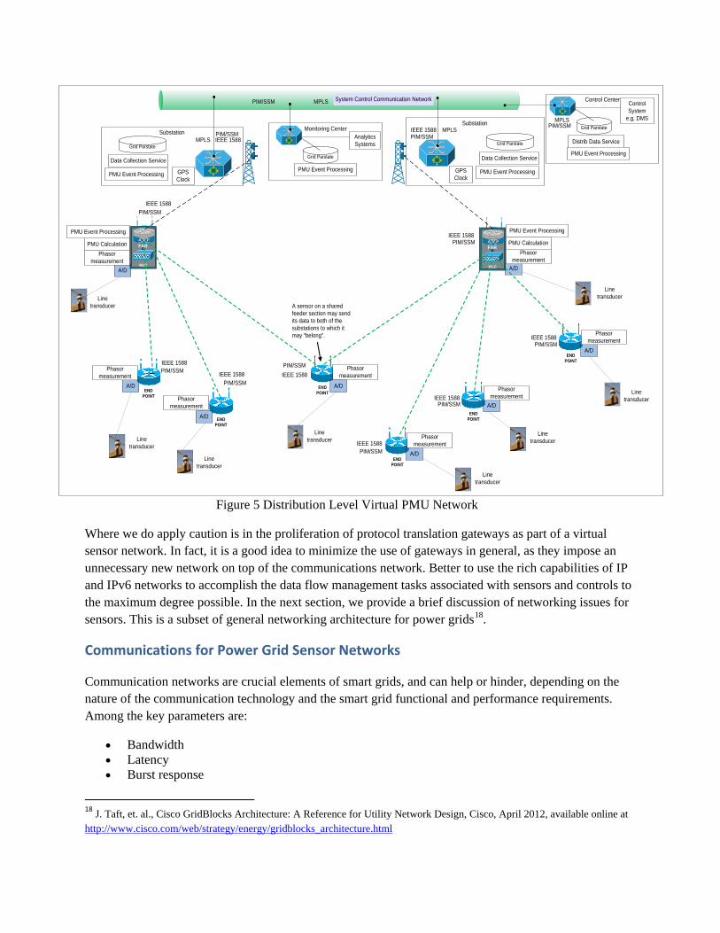
The term “sensor virtualization” has been used in several ways. In this paper it means the use of software or network services to allow more than one sensing node to act collectively as an abstract sensor, with unnecessary physical details hidden from application software that uses the sensor17. Sensor virtualization can be applied to reduce the cost of smart sensors in distribution grids by sharing computation capabilities for multiple physical transducers. This is especially valuable when deploying synchrophasor measurement capability on distribution feeders, where the cost of traditional PMU’s would be excessive. In some models, sensor network middleware is needed to implement the virtual sensor functions, but in practice network services could provide the requisite capabilities without the burden of a middleware layer. Figure 5 illustrates this concept, where multiple transducers coupled with digitizing capabilities acquire the necessary power waveform data, which is then streamed to a network node where computations transform waveforms to phasors. Applications can access the computation node, which can appear as one or several PMU’s. Since the exposed logical interface conceals physical details, the application does not need any knowledge of the individual nodes that connect to transducers, or the transducers themselves.
17 Anura P. Jayasumana, et. al., Virtual Sensor Networks – A Resource Efficient Approach for Concurrent Applications, IEEE Computer Society International Conference on Information Technology, 2007
SubstationSubstation
END POINT
END POINT
END POINT
D-SCADA
FAR
WLC
D-SCADA
FAR
WLC
END POINT
END POINT
END POINT
System Control Communication Network
PMU Calculation
IEEE 1588
IEEE 1588
IEEE 1588IEEE 1588
IEEE 1588
IEEE 1588
IEEE 1588
IEEE 1588
PIM/SSM
PIM/SSMPIM/SSM
PIM/SSM
PIM/SSM
PIM/SSM
PIM/SSM
PIM/SSM
IEEE 1588PIM/SSM
IEEE 1588PIM/SSM
GPS Clock
GPS Clock
PIM/SSM
Grid Parstate
Data Collection Service
PMU Calculation
A sensor on a shared feeder section may send its data to both of the substations to which it may “belong”.
Control Center Control System
e.g. DMSGrid Parstate
MPLS
MPLSMPLSMonitoring Center
Analytics Systems
Grid Parstate
MPLSPIM/SSM
A/D
A/D
A/D
A/D
A/D
A/D
A/D
Phasor measurement
A/D
Line transducer
Line transducer
Line transducer
Line transducer
Line transducer
Line transducer
Line transducer
Line transducer
PMU Event ProcessingPMU Event Processing
PMU Event Processing PMU Event Processing
Grid Parstate Distrib Data Service
PMU Event Processing
PMU Event Processing
Phasor measurement
Phasor measurement
Phasor measurement
Phasor measurement
Phasor measurement
Phasor measurement
Phasor measurement
Data Collection Service
Figure 5 Distribution Level Virtual PMU Network
Where we do apply caution is in the proliferation of protocol translation gateways as part of a virtual sensor network. In fact, it is a good idea to minimize the use of gateways in general, as they impose an unnecessary new network on top of the communications network. Better to use the rich capabilities of IP and IPv6 networks to accomplish the data flow management tasks associated with sensors and controls to the maximum degree possible. In the next section, we provide a brief discussion of networking issues for sensors. This is a subset of general networking architecture for power grids18.
Communications for Power Grid Sensor Networks
Communication networks are crucial elements of smart grids, and can help or hinder, depending on the nature of the communication technology and the smart grid functional and performance requirements. Among the key parameters are:
• Bandwidth • Latency • Burst response
18 J. Taft, et. al., Cisco GridBlocks Architecture: A Reference for Utility Network Design, Cisco, April 2012, available online at http://www.cisco.com/web/strategy/energy/gridblocks_architecture.html
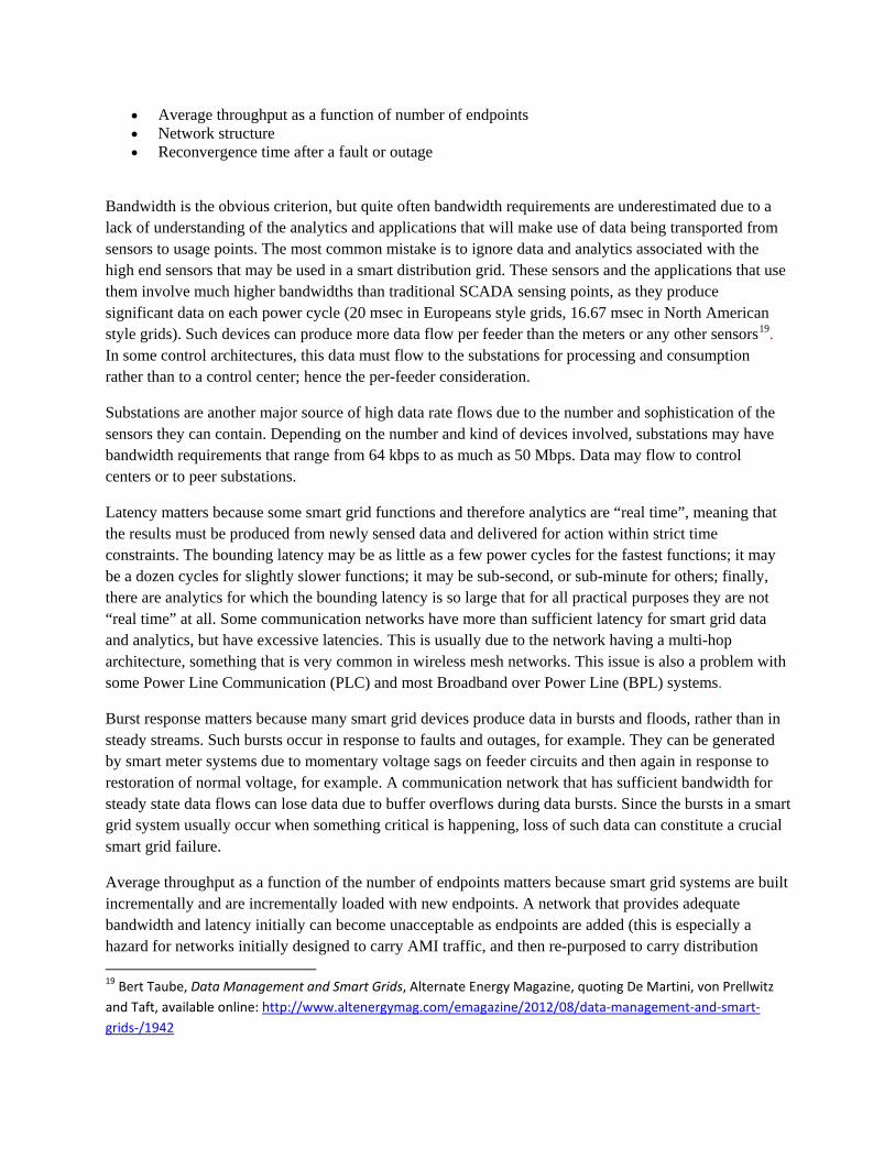
• Average throughput as a function of number of endpoints • Network structure • Reconvergence time after a fault or outage
Bandwidth is the obvious criterion, but quite often bandwidth requirements are underestimated due to a lack of understanding of the analytics and applications that will make use of data being transported from sensors to usage points. The most common mistake is to ignore data and analytics associated with the high end sensors that may be used in a smart distribution grid. These sensors and the applications that use them involve much higher bandwidths than traditional SCADA sensing points, as they produce significant data on each power cycle (20 msec in Europeans style grids, 16.67 msec in North American style grids). Such devices can produce more data flow per feeder than the meters or any other sensors19. In some control architectures, this data must flow to the substations for processing and consumption rather than to a control center; hence the per-feeder consideration.
Substations are another major source of high data rate flows due to the number and sophistication of the sensors they can contain. Depending on the number and kind of devices involved, substations may have bandwidth requirements that range from 64 kbps to as much as 50 Mbps. Data may flow to control centers or to peer substations.
Latency matters because some smart grid functions and therefore analytics are “real time”, meaning that the results must be produced from newly sensed data and delivered for action within strict time constraints. The bounding latency may be as little as a few power cycles for the fastest functions; it may be a dozen cycles for slightly slower functions; it may be sub-second, or sub-minute for others; finally, there are analytics for which the bounding latency is so large that for all practical purposes they are not “real time” at all. Some communication networks have more than sufficient latency for smart grid data and analytics, but have excessive latencies. This is usually due to the network having a multi-hop architecture, something that is very common in wireless mesh networks. This issue is also a problem with some Power Line Communication (PLC) and most Broadband over Power Line (BPL) systems.
Burst response matters because many smart grid devices produce data in bursts and floods, rather than in steady streams. Such bursts occur in response to faults and outages, for example. They can be generated by smart meter systems due to momentary voltage sags on feeder circuits and then again in response to restoration of normal voltage, for example. A communication network that has sufficient bandwidth for steady state data flows can lose data due to buffer overflows during data bursts. Since the bursts in a smart grid system usually occur when something critical is happening, loss of such data can constitute a crucial smart grid failure.
Average throughput as a function of the number of endpoints matters because smart grid systems are built incrementally and are incrementally loaded with new endpoints. A network that provides adequate bandwidth and latency initially can become unacceptable as endpoints are added (this is especially a hazard for networks initially designed to carry AMI traffic, and then re-purposed to carry distribution 19 Bert Taube, Data Management and Smart Grids, Alternate Energy Magazine, quoting De Martini, von Prellwitz and Taft, available online: http://www.altenergymag.com/emagazine/2012/08/data-management-and-smart-grids-/1942
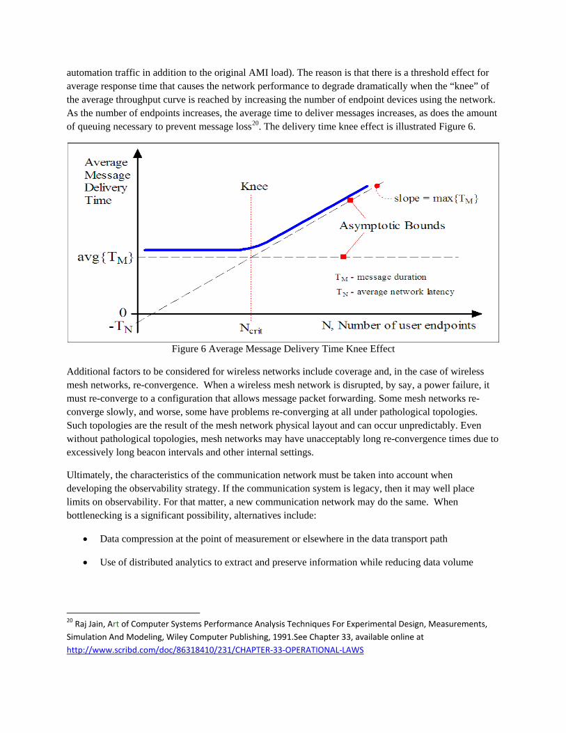
automation traffic in addition to the original AMI load). The reason is that there is a threshold effect for average response time that causes the network performance to degrade dramatically when the “knee” of the average throughput curve is reached by increasing the number of endpoint devices using the network. As the number of endpoints increases, the average time to deliver messages increases, as does the amount of queuing necessary to prevent message loss20. The delivery time knee effect is illustrated Figure 6.
Figure 6 Average Message Delivery Time Knee Effect
Additional factors to be considered for wireless networks include coverage and, in the case of wireless mesh networks, re-convergence. When a wireless mesh network is disrupted, by say, a power failure, it must re-converge to a configuration that allows message packet forwarding. Some mesh networks re-converge slowly, and worse, some have problems re-converging at all under pathological topologies. Such topologies are the result of the mesh network physical layout and can occur unpredictably. Even without pathological topologies, mesh networks may have unacceptably long re-convergence times due to excessively long beacon intervals and other internal settings.
Ultimately, the characteristics of the communication network must be taken into account when developing the observability strategy. If the communication system is legacy, then it may well place limits on observability. For that matter, a new communication network may do the same. When bottlenecking is a significant possibility, alternatives include:
• Data compression at the point of measurement or elsewhere in the data transport path
• Use of distributed analytics to extract and preserve information while reducing data volume
20 Raj Jain, Art of Computer Systems Performance Analysis Techniques For Experimental Design, Measurements, Simulation And Modeling, Wiley Computer Publishing, 1991.See Chapter 33, available online at http://www.scribd.com/doc/86318410/231/CHAPTER-33-OPERATIONAL-LAWS

The consequences of these approaches are increases in the computation power at endpoints, potential additional data security issues, and new requirements for management of distributed software and smart devices.
A great many considerations go into the design of communications networks for power grids, too many to go into here. It is worth noting that a very rich set of advanced protocols is available in IPv6-based networks, as well and variety of application-oriented protocols have emerged in the context of advanced power grid functions. These protocols can be used to do more than just provide data pipes; they can manage data flows, provide network-level security, and facilitate system integration. It is important to align communication network capabilities to power grid requirements and to avoid mismatches. Strong and comprehensive reference architecture is crucial in this regard; it provides the full context for any or all parts of a utility communication solution, including the sensing and measurement sub-system.
Observability Strategy
Sensing and measurement support multiple purposes in the smart grid environment and this applies equally as well to many other systems characterized by either geographic dispersal, or large numbers of ends points, especially when some form of control is required. Consequently, the sensing system design can be quite complex, involving issues such as physical parameter selection, sensor mix and placement optimization, measurement type and sample rate, data conversion, sensor calibration, and compensation for non-ideal sensor characteristics.
We may divide sensor networks into three classes:
• Type 1: those for which there is a physical presence but no particular underlying structure (such as battlefield surveillance networks)
• Type 2: those for which there is an underlying structured physical system (such as power grid sensor networks)
• Type 3: those for which there is no relevant physical system but there is a cyber system, such as financial networks and social networks
Type 1 networks usually must provide general coverage of a target zone or area and so the topological concept of homology groups becomes a useful tool to determine coverage gaps21, which is a key issue with most applications involving Type 1 sensor nets. We will not discuss such networks any further here as they are not very useful in the utility setting.
With Type 2 networks, we may take another approach based on the topological structure of the underlying physical system and the concept of system state. This means we do not need to resort to the concept of ad hoc randomly distributed meshes for Type 1 sensor networks. Instead, for Type 2 networks, we employ the ideas of system state and observability, combined with an understanding of how the sensor
21 Vin De Silva and Robert Ghrist, Coverage in Sensor Networks via Persistent Homology, Algebraic and Geometric Topology, 7 (2007), pp 339 – 358. available online at msp.org/agt/2007/07/agt-2007-07-016s.pdf
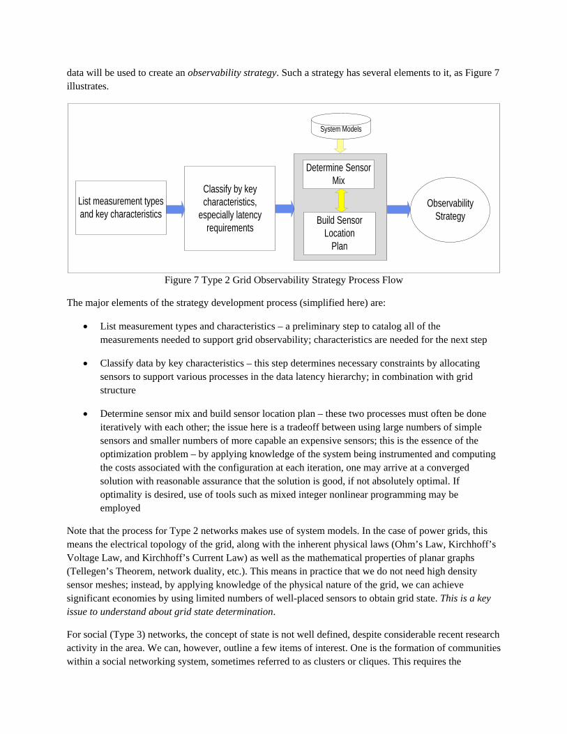
data will be used to create an observability strategy. Such a strategy has several elements to it, as Figure 7 illustrates.
Classify by key characteristics,
especially latency requirements
Determine SensorMix
Build Sensor Location
Plan
List measurement typesand key characteristics
ObservabilityStrategy
System Models
Figure 7 Type 2 Grid Observability Strategy Process Flow
The major elements of the strategy development process (simplified here) are:
• List measurement types and characteristics – a preliminary step to catalog all of the measurements needed to support grid observability; characteristics are needed for the next step
• Classify data by key characteristics – this step determines necessary constraints by allocating sensors to support various processes in the data latency hierarchy; in combination with grid structure
• Determine sensor mix and build sensor location plan – these two processes must often be done iteratively with each other; the issue here is a tradeoff between using large numbers of simple sensors and smaller numbers of more capable an expensive sensors; this is the essence of the optimization problem – by applying knowledge of the system being instrumented and computing the costs associated with the configuration at each iteration, one may arrive at a converged solution with reasonable assurance that the solution is good, if not absolutely optimal. If optimality is desired, use of tools such as mixed integer nonlinear programming may be employed
Note that the process for Type 2 networks makes use of system models. In the case of power grids, this means the electrical topology of the grid, along with the inherent physical laws (Ohm’s Law, Kirchhoff’s Voltage Law, and Kirchhoff’s Current Law) as well as the mathematical properties of planar graphs (Tellegen’s Theorem, network duality, etc.). This means in practice that we do not need high density sensor meshes; instead, by applying knowledge of the physical nature of the grid, we can achieve significant economies by using limited numbers of well-placed sensors to obtain grid state. This is a key issue to understand about grid state determination.
For social (Type 3) networks, the concept of state is not well defined, despite considerable recent research activity in the area. We can, however, outline a few items of interest. One is the formation of communities within a social networking system, sometimes referred to as clusters or cliques. This requires the
discovery of logical connectivity, which parallels the power grid issue of electrical connectivity discovery and here we should make a distinction between social networking services, and the actual social networks that form on them. Various techniques are being explored to detect the existence of communities to measure their extents. The research on this is spread over a wide variety of disciplines22,23. It is not clear that specific criteria exist for determining the observability of a social network as of this writing.
Other activity has focused on understanding social network dynamics, as measured via economic activity like online bidding and other resource allocation and cooperation/competition interactions, using information theory and game theory as tools24. Another approach to social networks has been to mine them for information as if they constitute sensor networks themselves. An experimental effort in this direction is being carried out by the US Geologic Survey in attempting to use Twitter to detect and locate earthquakes25.
It is clear that social networks are part of the multi-network convergence involved in smart grid evolution, but more remains to be done to fully exploit this for measurement purposes.
Sensor Allocation
A key aspect of observability strategy and resultant sensor network design is the allocation of sensors: determination of appropriate sensors types and selecting the number and locations of the sensors. If sensors, sensor communications networks, and installation were all negligible cost, then one might just over-instrument a grid. However, this certainly not the case and even if the sensors were free, the cost to install them at arbitrarily high density would be prohibitive. This leads to a significant issue of sensor allocation optimization, which leads back to the use of the structural properties of Type 2 sensor networks.
Transmission
Transmission grid state has traditionally been estimated from a system model and a sparse set of state variable measurements. More recently, PMU’s have been added to the transmission grids in North America and other countries for a variety of purposes but including improvement of grid observability. A number of studies have been carried out on optimal number and placement of PMU’s on transmission systems. This has led to a design guideline that is suitable for observability strategy purposes: PMU’s are needed on 1/3 of the buses in a transmission system to ensure complete observability [ref]. One must still carry out the design process to determine the optimal locations of these PMU’s, but the guideline provides 22 M.E.J. Newman and M. Girvan, Finding and Evaluating Community Structure in Networks, Physics Rev E, vol. 69, no. 2, 2004
23 M. Rosvall and C. T. Bergstrom, An Information-Theoretic Framework for Resolving Community Structure in Complex Networks, Proc. Nat. Acad. Sci. USA, vol. 104, No. 18, pp. 7327-731, 2007
24 Yan Chen and K. J. Ray Liu, Understanding Microeconomic Behaviors in Social Networking, IEEE Signal Processing Magazine, March 2012, pp. 53-64
25 See the USGS website page at http://recovery.doi.gov/press/us-geological-survey-twitter-earthquake-detector-ted/
a key number. Engineers may decide that additional PMU’s are needed or useful, so the guideline is just a starting point for the transmission observability strategy, and engineering knowledge of the system under consideration plus additional analysis may be need to handle unique cases. In addition, other sensors in the transmission substations or even on the transmission lines may be included in the sensor mix, reducing the total number of PMU’s to be used. Such tradeoffs are essential to the development of the observability strategy.
Distribution
Observability for distribution grids is fundamentally a more difficult issue than for transmission for all but the simplest radial systems. Complicating factors include feeder branches and laterals, unbalanced circuits, poorly documented circuits, large numbers of attached loads and devices and, in the case of feeders with inter-ties, time-varying circuit topology. In general, circuit topology and device electrical connectivity may be poorly (incompletely or inaccurately or both) known. These issues make state estimation more difficult than for transmission systems, so it is necessary to rely more upon state measurement and less on estimation.
Sensors for distribution grids may be organized into three tiers. The top tier includes feeder sensing devices such as waveform recorders, digital relays, and PMU’s located in the primary distribution substations. This tier also contains sensing for asset monitoring and power quality measurement.
The second tier includes devices located on feeders outside of the primary substations. We shall consider five classes of devices at this tier:
1. Binary devices, such as Faulted Circuit Indicators (FCI’s) – these devices indicate events such as the passage of a fault current at the sensing point
2. Line sensors – use analog transducers and digital processing to extract parameters from voltage and current waveforms, but measurements are not synchronized across the system
3. Distribution PMU’s – distribution level phasor measurement units that extract current and voltage phasors that are synchronized across the system
4. Waveform recorders – these devices record waveforms with much denser sampling than other sensors, in order to capture high speed transient and high order harmonic information. Devices include power quality monitors and transient event recorders. They may record continually or may be triggered by grid events to retain a window of waveform data leading up to, including, and trailing the event.
5. Grid device controllers – many grid devices such as capacitor banks have controllers that have electrical sensing capabilities; they may be useful as sensing devices when they can be networked to the communication system
The third tier includes devices connected to the feeder secondary, such as meters and frequency disturbance monitors. Figure 8 illustrates this sensing hierarchy. It is important to understand the performance characteristics of each sensor type, especially the rate at which data can be extracted from them. This allows one to match sensor types against latency requirements for the various data classes to
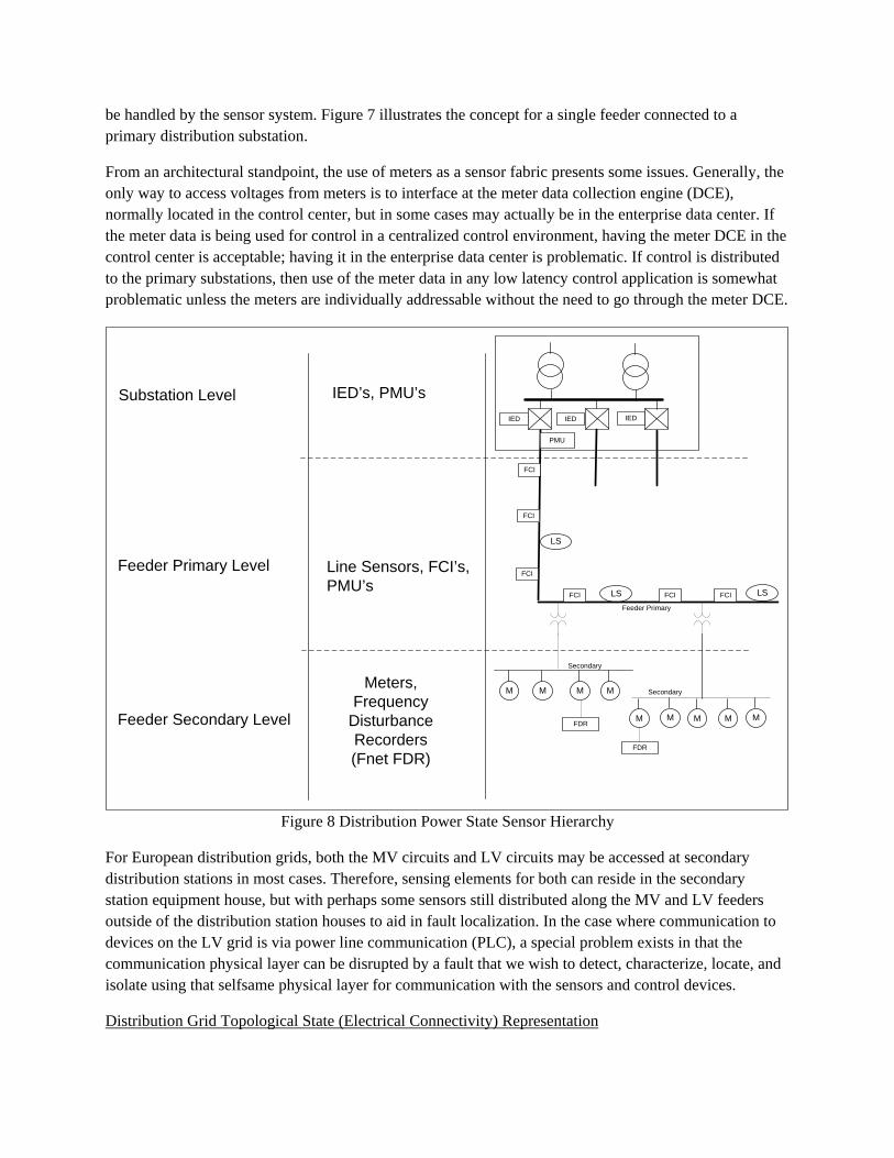
be handled by the sensor system. Figure 7 illustrates the concept for a single feeder connected to a primary distribution substation.
From an architectural standpoint, the use of meters as a sensor fabric presents some issues. Generally, the only way to access voltages from meters is to interface at the meter data collection engine (DCE), normally located in the control center, but in some cases may actually be in the enterprise data center. If the meter data is being used for control in a centralized control environment, having the meter DCE in the control center is acceptable; having it in the enterprise data center is problematic. If control is distributed to the primary substations, then use of the meter data in any low latency control application is somewhat problematic unless the meters are individually addressable without the need to go through the meter DCE.
Substation Level
Feeder Primary Level
Feeder Secondary Level
IED’s, PMU’s
Line Sensors, FCI’s,PMU’s
Meters, Frequency
Disturbance Recorders (Fnet FDR)
LS LS
LS
FCIFCI
FCI
Secondary
Feeder Primary
IEDIED IED
M M M M
FDR
FCI
FCI
FCI
M M M M M
FDR
Secondary
PMU
Figure 8 Distribution Power State Sensor Hierarchy
For European distribution grids, both the MV circuits and LV circuits may be accessed at secondary distribution stations in most cases. Therefore, sensing elements for both can reside in the secondary station equipment house, but with perhaps some sensors still distributed along the MV and LV feeders outside of the distribution station houses to aid in fault localization. In the case where communication to devices on the LV grid is via power line communication (PLC), a special problem exists in that the communication physical layer can be disrupted by a fault that we wish to detect, characterize, locate, and isolate using that selfsame physical layer for communication with the sensors and control devices.
Distribution Grid Topological State (Electrical Connectivity) Representation
Distribution grids present special problems in terms of topological state. Such state information is crucial because it is the context in which grid data, events and control commands must be interpreted. The problems arise because unlike transmission grids, “as-built” topology for distribution grids is often not completely or accurately known. In addition, distribution grid topology can be dynamic, such as in the cases where feeders are partially meshed or are tied to other feeders for reliability reasons. In such cases, circuit switches, sectionalizers, or reclosers may be operated to change the topology and such changes can be frequent. Consequently, data flows in a given circuit section can reverse, as can voltage rises and drops. With the advent of Distributed Generation (DG) penetration on distribution feeders, power flow reversals and loops can occur, impacting protection and Volt/VAr regulation.
Due to grid switching, a feeder section may “belong” to more than one feeder or substation. This raises several issues: how to obtain real time circuit topology, how to represent power state for such sections (since power state must refer to circuit topology), and how to handle distributed sensor data acquisition (which of the several distributed DCE’s should collect the data from a section that can belong to more than one substation, for example).
The issue of circuit topology determination is one of the hidden issues for smart grid design, because it can undermine much of the advanced capabilities that smart grids are intended to achieve and yet the issue is often not discussed or included in the sensor system design process. Furthermore, it is not sufficient to have topological state on a current operational data basis (meaning the present value). This is because data may not always be interpreted or acted upon immediately. If there is a processing delay, circuit topology may change in between the time the data or event message was generated and the time when the data is processed or the time that a control command is issued. Therefore, past values of topological state are needed in order to provide the correct context for the data, whereas present values are needed to provide context for control commands.
One method of providing the multiple versions of topology that are needed for advanced grid control is to capture the state changes of grid switches, reclosers, sectionalizers, and inter-ties in a time series database and then use a topology processor to reconstruct topology for any required present or past time. The collection of these state transitions is often problematic because the switching device may not report back its state and also because the device may malfunction. In addition, not all switching devices are automatic – many distribution grids contain large numbers of manually-operated switches. Capture of state transitions for such devices is problematic, but can be resolved with a degree of line sensing designed to provide measurement of power state variables that allow automatic inference of the switch state transitions (by sensing changes in line voltage or current flow). If switch state transition determination is an issue, then an aspect of observability strategy should be to include means to sense those changes.
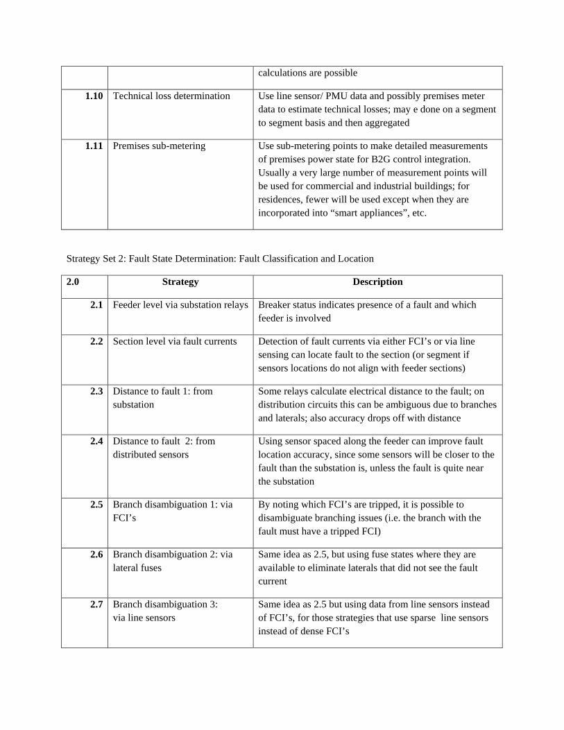
Sensing Sub-Strategies
The following tables contain elements of a number of sub-strategies for power grid observability. These can be used to assemble key portions of an overall observability strategy and sensor network design.

Strategy Set 1: Power State Determination
1.0 Strategy Description
1.1 Sparse SCADA sampling Standard method for old-style SCADA; use a very limited number of sensing points (one or two per feeder); for more detailed sensing, three to five per feeder is normally sufficient, but consider Figure 9 below to deal with branches and laterals
1.2 Synchrophasor sampling Deploy PMU’s at the feeder head end in the primary substation, as well as at three to five points along the feeder
1.3 Premises meter sampling Use addressable meters to provide voltage profiles along a feeder – 10 to 20 meters are sufficient, but plan to have alternates in case a given meter does not communicate on demand
1.4 Heterogeneous sampling Use a mixture of sensor types to assemble grid state, including line sensors, PMU’s , meters
1.5 Rollup and aggregation Aggregate point level grid state measurements into section, feeder, substation level state elements by a combining power summations with head end voltage readings; currents may be summed provided every branch is accounted for
1.6 DG Power Flow Monitoring Monitor power flow at the Point of Coupling on the grid side for distributed generation; alternate – obtain the data from the DG controller
1.7 DS energy state Obtain state of charge of distributed storage units from DS controllers
1.7 DR Available Capacity Estimate available DR capacity for the next market period based on statistical models and available behavioral data
1.8 Circuit parameters via PMU’s Use PMU’s in a pair-wise fashion to estimate circuit paramete3s for the circuit segment between the PMU’s; care must be taken on distribution circuits as phase shifts can be quite small and measurements can be noisy – the resultant calculations can be ill-conditioned
1.9 Circuit parameters via meters The same idea as above, but using only meter measurements – the problem is that where meters do not measure phase angle (usually the case) only magnitude
calculations are possible
1.10 Technical loss determination Use line sensor/ PMU data and possibly premises meter data to estimate technical losses; may e done on a segment to segment basis and then aggregated
1.11 Premises sub-metering Use sub-metering points to make detailed measurements of premises power state for B2G control integration. Usually a very large number of measurement points will be used for commercial and industrial buildings; for residences, fewer will be used except when they are incorporated into “smart appliances”, etc.
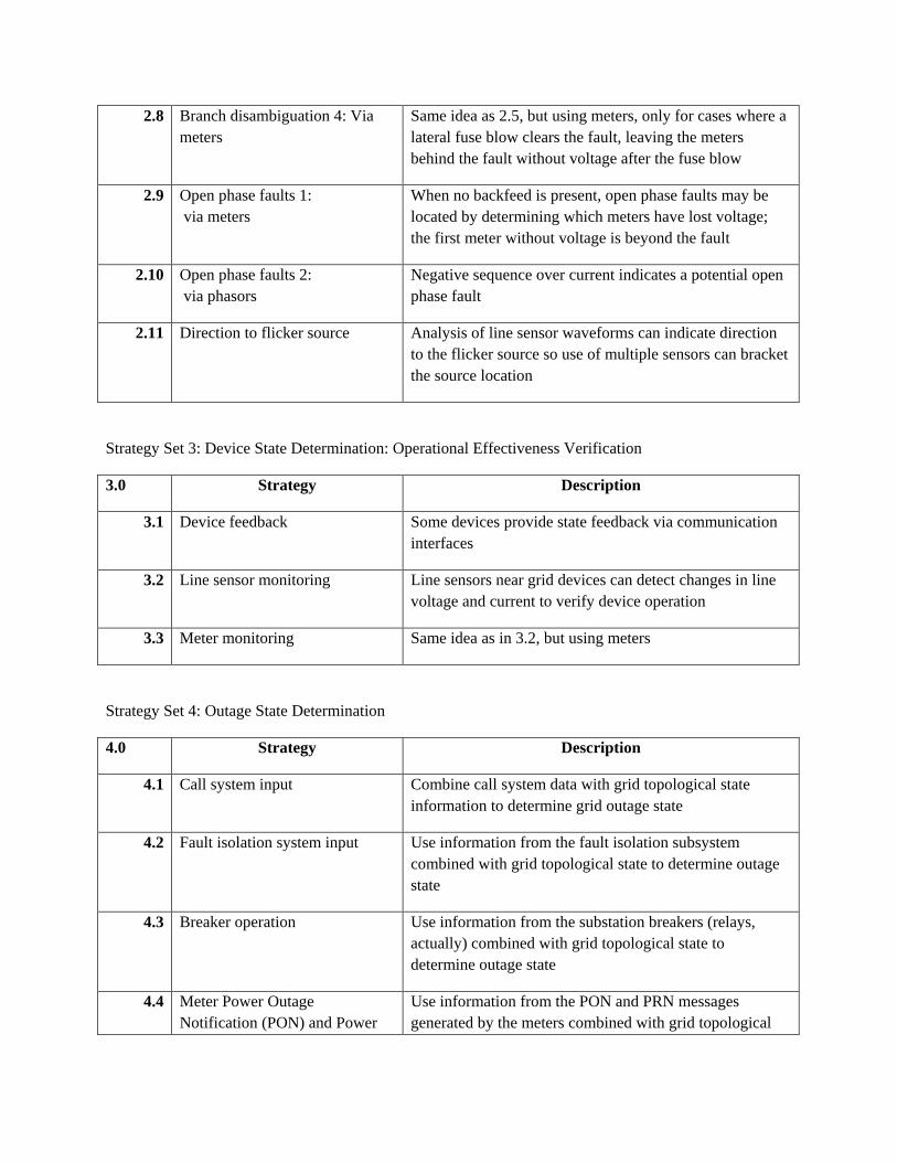
Strategy Set 2: Fault State Determination: Fault Classification and Location
2.0 Strategy Description
2.1 Feeder level via substation relays Breaker status indicates presence of a fault and which feeder is involved
2.2 Section level via fault currents Detection of fault currents via either FCI’s or via line sensing can locate fault to the section (or segment if sensors locations do not align with feeder sections)
2.3 Distance to fault 1: from substation
Some relays calculate electrical distance to the fault; on distribution circuits this can be ambiguous due to branches and laterals; also accuracy drops off with distance
2.4 Distance to fault 2: from distributed sensors
Using sensor spaced along the feeder can improve fault location accuracy, since some sensors will be closer to the fault than the substation is, unless the fault is quite near the substation
2.5 Branch disambiguation 1: via FCI’s
By noting which FCI’s are tripped, it is possible to disambiguate branching issues (i.e. the branch with the fault must have a tripped FCI)
2.6 Branch disambiguation 2: via lateral fuses
Same idea as 2.5, but using fuse states where they are available to eliminate laterals that did not see the fault current
2.7 Branch disambiguation 3: via line sensors
Same idea as 2.5 but using data from line sensors instead of FCI’s, for those strategies that use sparse line sensors instead of dense FCI’s
2.8 Branch disambiguation 4: Via meters
Same idea as 2.5, but using meters, only for cases where a lateral fuse blow clears the fault, leaving the meters behind the fault without voltage after the fuse blow
2.9 Open phase faults 1: via meters
When no backfeed is present, open phase faults may be located by determining which meters have lost voltage; the first meter without voltage is beyond the fault
2.10 Open phase faults 2: via phasors
Negative sequence over current indicates a potential open phase fault
2.11 Direction to flicker source Analysis of line sensor waveforms can indicate direction to the flicker source so use of multiple sensors can bracket the source location
Strategy Set 3: Device State Determination: Operational Effectiveness Verification
3.0 Strategy Description
3.1 Device feedback Some devices provide state feedback via communication interfaces
3.2 Line sensor monitoring Line sensors near grid devices can detect changes in line voltage and current to verify device operation
3.3 Meter monitoring Same idea as in 3.2, but using meters
Strategy Set 4: Outage State Determination
4.0 Strategy Description
4.1 Call system input Combine call system data with grid topological state information to determine grid outage state
4.2 Fault isolation system input Use information from the fault isolation subsystem combined with grid topological state to determine outage state
4.3 Breaker operation Use information from the substation breakers (relays, actually) combined with grid topological state to determine outage state
4.4 Meter Power Outage Notification (PON) and Power
Use information from the PON and PRN messages generated by the meters combined with grid topological
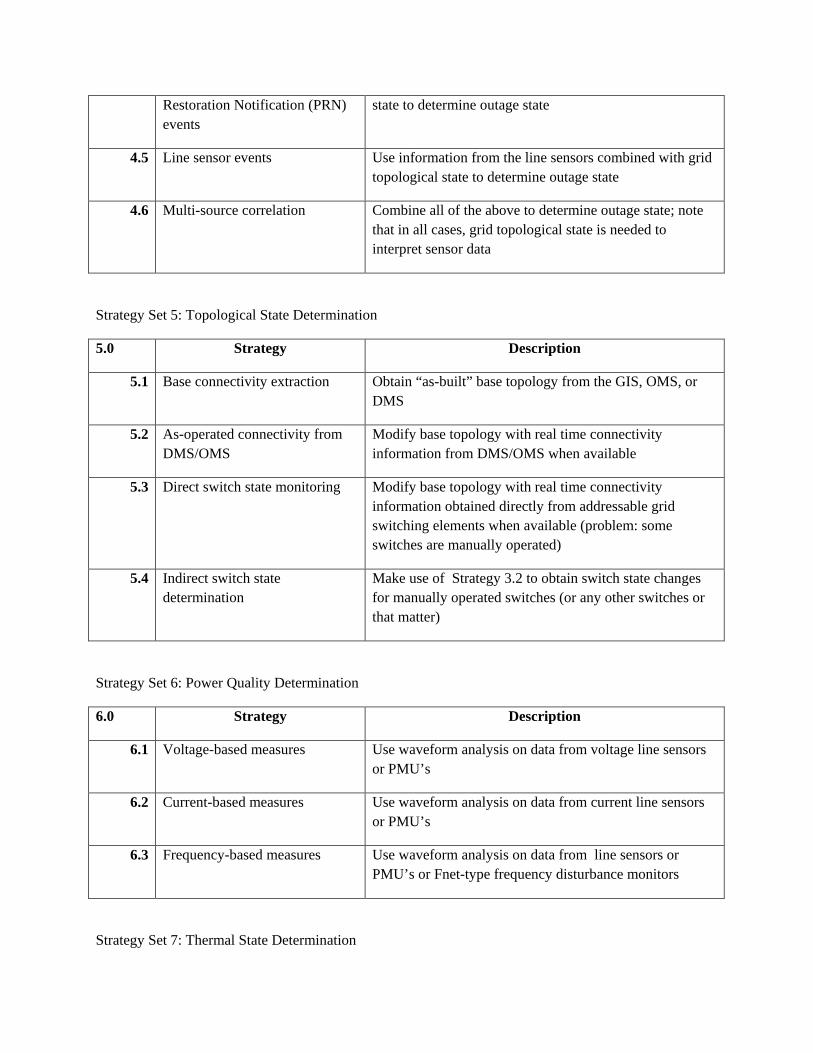
Restoration Notification (PRN) events
state to determine outage state
4.5 Line sensor events Use information from the line sensors combined with grid topological state to determine outage state
4.6 Multi-source correlation Combine all of the above to determine outage state; note that in all cases, grid topological state is needed to interpret sensor data
Strategy Set 5: Topological State Determination
5.0 Strategy Description
5.1 Base connectivity extraction Obtain “as-built” base topology from the GIS, OMS, or DMS
5.2 As-operated connectivity from DMS/OMS
Modify base topology with real time connectivity information from DMS/OMS when available
5.3 Direct switch state monitoring Modify base topology with real time connectivity information obtained directly from addressable grid switching elements when available (problem: some switches are manually operated)
5.4 Indirect switch state determination
Make use of Strategy 3.2 to obtain switch state changes for manually operated switches (or any other switches or that matter)
Strategy Set 6: Power Quality Determination
6.0 Strategy Description
6.1 Voltage-based measures Use waveform analysis on data from voltage line sensors or PMU’s
6.2 Current-based measures Use waveform analysis on data from current line sensors or PMU’s
6.3 Frequency-based measures Use waveform analysis on data from line sensors or PMU’s or Fnet-type frequency disturbance monitors
Strategy Set 7: Thermal State Determination
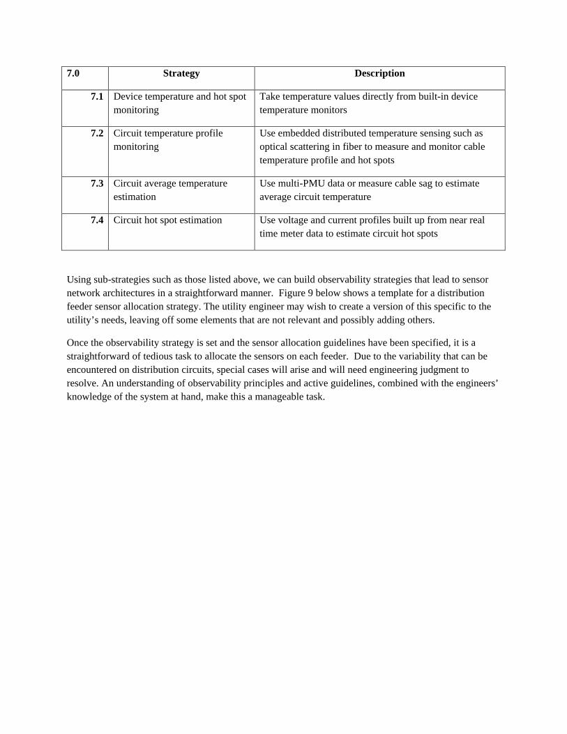
7.0 Strategy Description
7.1 Device temperature and hot spot monitoring
Take temperature values directly from built-in device temperature monitors
7.2 Circuit temperature profile monitoring
Use embedded distributed temperature sensing such as optical scattering in fiber to measure and monitor cable temperature profile and hot spots
7.3 Circuit average temperature estimation
Use multi-PMU data or measure cable sag to estimate average circuit temperature
7.4 Circuit hot spot estimation Use voltage and current profiles built up from near real time meter data to estimate circuit hot spots
Using sub-strategies such as those listed above, we can build observability strategies that lead to sensor network architectures in a straightforward manner. Figure 9 below shows a template for a distribution feeder sensor allocation strategy. The utility engineer may wish to create a version of this specific to the utility’s needs, leaving off some elements that are not relevant and possibly adding others.
Once the observability strategy is set and the sensor allocation guidelines have been specified, it is a straightforward of tedious task to allocate the sensors on each feeder. Due to the variability that can be encountered on distribution circuits, special cases will arise and will need engineering judgment to resolve. An understanding of observability principles and active guidelines, combined with the engineers’ knowledge of the system at hand, make this a manageable task.
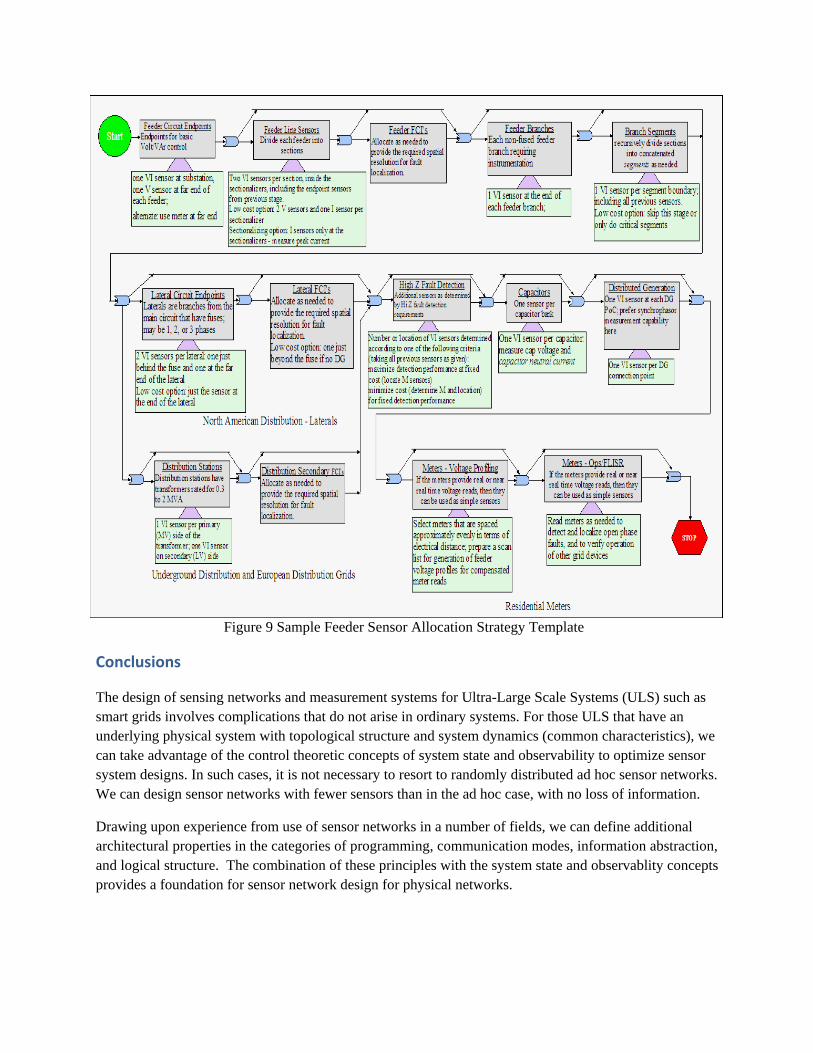
Figure 9 Sample Feeder Sensor Allocation Strategy Template
Conclusions
The design of sensing networks and measurement systems for Ultra-Large Scale Systems (ULS) such as smart grids involves complications that do not arise in ordinary systems. For those ULS that have an underlying physical system with topological structure and system dynamics (common characteristics), we can take advantage of the control theoretic concepts of system state and observability to optimize sensor system designs. In such cases, it is not necessary to resort to randomly distributed ad hoc sensor networks. We can design sensor networks with fewer sensors than in the ad hoc case, with no loss of information.
Drawing upon experience from use of sensor networks in a number of fields, we can define additional architectural properties in the categories of programming, communication modes, information abstraction, and logical structure. The combination of these principles with the system state and observablity concepts provides a foundation for sensor network design for physical networks.