Semiparametric GEE analysis in partially linear single ... · 2 CHEN, LI, LIANG AND WANG with dimensions d and p, respectively, and e(t) is the random error process. For the case

arX

iv:1

507.

0847

3v1

[m

ath.

ST]

30

Jul 2

015

The Annals of Statistics

2015, Vol. 43, No. 4, 1682–1715DOI: 10.1214/15-AOS1320c© Institute of Mathematical Statistics, 2015

SEMIPARAMETRIC GEE ANALYSIS IN PARTIALLY LINEAR

SINGLE-INDEX MODELS FOR LONGITUDINAL DATA

By Jia Chen∗, Degui Li∗, Hua Liang†,1 and Suojin Wang‡,2

University of York∗, George Washington University† and Texas A&MUniversity‡

In this article, we study a partially linear single-index model forlongitudinal data under a general framework which includes both thesparse and dense longitudinal data cases. A semiparametric estima-tion method based on a combination of the local linear smoothingand generalized estimation equations (GEE) is introduced to esti-mate the two parameter vectors as well as the unknown link func-tion. Under some mild conditions, we derive the asymptotic prop-erties of the proposed parametric and nonparametric estimators indifferent scenarios, from which we find that the convergence ratesand asymptotic variances of the proposed estimators for sparse lon-gitudinal data would be substantially different from those for denselongitudinal data. We also discuss the estimation of the covariance (orweight) matrices involved in the semiparametric GEE method. Fur-thermore, we provide some numerical studies including Monte Carlosimulation and an empirical application to illustrate our methodologyand theory.

1. Introduction. Consider a semiparametric partially linear single-indexmodel defined by

Y (t) =Z⊤(t)β + η(X⊤(t)θ) + e(t), t ∈ T ,(1.1)

where T is a bounded time interval, β and θ are two unknown vectors ofparameters with dimensions d and p, respectively, η(·) is an unknown linkfunction, Y (t) is a scalar stochastic process, Z(t) and X(t) are covariates

Received May 2014; revised February 2015.1Supported in part by NSF Grants DMS-14-40121 and DMS-14-18042 and by Award

Number 11228103, made by National Natural Science Foundation of China.2Supported in part by Award Number KUS-CI-016-04, made by King Abdullah Uni-

versity of Science and Technology (KAUST).AMS 2000 subject classifications. 62G09, 62H99, 62G99.Key words and phrases. Efficiency, GEE, local linear smoothing, longitudinal data,

semiparametric estimation, single-index models.

This is an electronic reprint of the original article published by theInstitute of Mathematical Statistics in The Annals of Statistics,2015, Vol. 43, No. 4, 1682–1715. This reprint differs from the original inpagination and typographic detail.

1

http://arxiv.org/abs/1507.08473v1

http://www.imstat.org/aos/

http://dx.doi.org/10.1214/15-AOS1320

http://www.imstat.org

http://www.ams.org/msc/

http://www.imstat.org

http://www.imstat.org/aos/

http://dx.doi.org/10.1214/15-AOS1320

2 CHEN, LI, LIANG AND WANG

with dimensions d and p, respectively, and e(t) is the random error process.For the case of independent and identically distributed (i.i.d.) or weakly de-pendent time series data, there has been extensive literature on statisticalinference of model (1.1) since its introduction by Carroll et al. (1997). Severaldifferent approaches have been proposed to estimate the unknown parame-ters and link function involved; see, for example, Xia, Tong and Li (1999),Yu and Ruppert (2002), Xia and Hardle (2006), Wang et al. (2010) and Maand Zhu (2013). A recent paper by Liang et al. (2010) further developedsemiparametric techniques for the variable selection and model specificationtesting issues in the context of model (1.1).

In this paper, we are interested in studying partially linear single-indexmodel (1.1) in the context of longitudinal data which arise frequently inmany fields of research, such as biology, climatology, economics and epi-demiology, and thus have attracted considerable attention in the literaturein recent years. Various parametric models and methods have been studiedin depth for longitudinal data; see Diggle et al. (2002) and the referencestherein. However, the parametric models may be misspecified in practice,and the misspecification may lead to inconsistent estimates and incorrectconclusions being drawn. Hence, to circumvent this issue, in recent years,there has been a large literature on how to relax the parametric assumptionson longitudinal data models and many nonparametric, and semiparametricmodels have thus been investigated; see, for example, Lin and Ying (2001),He, Zhu and Fung (2002), Fan and Li (2004), Wang, Carroll and Lin (2005),Lin and Carroll (2006), Wu and Zhang (2006), Li and Hsing (2010), Jiangand Wang (2011) and Yao and Li (2013).

Suppose that we have a random sample with n subjects from model (1.1).For the ith subject, i= 1, . . . , n, the response variable Yi(t) and the covari-ates Zi(t),Xi(t) are collected at random time points tij , j = 1, . . . ,mi,which are distributed in a bounded time interval T according to the prob-ability density function fT (t). Here mi is the total number of observationsfor the ith subject. To accommodate such longitudinal data, model (1.1) iswritten in the following framework:

Yi(tij) = Z⊤i (tij)β+ η(X⊤

i (tij)θ) + ei(tij)(1.2)

for i = 1, . . . , n and j = 1, . . . ,mi. When mi varies across the subjects, thelongitudinal data set under investigation is unbalanced. Several nonpara-metric and semiparametric models can be viewed as special cases of model(1.2). For instance, when β = 0, model (1.2) reduces to the single-index lon-gitudinal data model [Jiang and Wang (2011), Chen, Gao and Li (2013a)];when p= 1 and θ = 1, model (1.2) reduces to the partially linear longitudi-nal data model [Fan and Li (2004)]. To avoid confusion, we let β0 and θ0 bethe true values of the two parameter vectors. For identifiability reasons, θ0

PARTIALLY LINEAR SINGLE-INDEX MODELS 3

is assumed to be a unit vector with the first nonzero element being positive.Furthermore, we allow that there exists certain within-subject correlationstructure for ei(tij), which makes the model assumption more realistic butthe development of estimation methodology more challenging.

To estimate the parameters β0, θ0 as well as the link function η(·) inmodel (1.2), we first apply the local linear approximation to the unknownlink function, and then introduce a profile weighted least squares approachto estimate the two parameter vectors based on the technique of general-ized estimation equations (GEE). Under some mild conditions, we derivethe asymptotic properties of the developed parametric and nonparametricestimators in different scenarios. Our framework is flexible in that mi caneither be bounded or tend to infinity. Thus both the dense and sparse lon-gitudinal data cases can be included. Dense longitudinal data means thatthere exists a sequence of positive numbers Mn such that minimi ≥Mn, andMn →∞ as n→∞ [see, e.g., Hall, Muller and Wang (2006) and Zhang andChen (2007)], whereas sparse longitudinal data means that there exists apositive constant M∗ such that maximi ≤M∗; see, for example, Yao, Mullerand Wang (2005), Wang, Qian and Carroll (2010). We show that the conver-gence rates and asymptotic variances of our semiparametric estimators inthe sparse case are substantially different from those in the dense case. Fur-thermore, we show that the proposed semiparametric GEE (SGEE)-basedestimators are asymptotically more efficient than the profile unweighted leastsquares (PULS) estimators, when the weights in the SGEE method are cho-sen as the inverse of the covariance matrix of the errors. We also introducea semiparametric approach to estimate the covariance matrices (or weights)involved in the SGEE method, which is based on a variance–correlation de-composition and consists of two steps: first, estimate the conditional variancefunction using a robust nonparametric method that accommodates heavy-tailed errors, and second, estimate the parameters in the correlation matrix.A simulation study and a real data analysis are provided to illustrate ourmethodology and theory.

The rest of the paper is organized as follows. In Section 2, we introducethe SGEE methodology for estimating β0, θ0 and η(·). Section 3 establishesthe large sample theory for the proposed parametric and nonparametricestimators and gives some related discussions. Section 4 discusses how todetermine the weight matrices in the estimation equations. Section 5 givessome numerical examples to investigate the finite sample performance ofthe proposed approach. Section 6 concludes the paper. Technical assump-tions are given in Appendix A. The proofs of the main results are given inAppendix B. Some auxiliary lemmas and their proofs are provided in thesupplementary material [Chen et al. (2015)].


2. Estimation methodology. Various semiparametric estimationapproaches have been proposed to estimate model (1.1) in the case of i.i.d. ob-servations (or weakly dependent time series data). See, for example, Carrollet al. (1997) and Liang et al. (2010) for the profile likelihood method, Yuand Ruppert (2002) and Wang et al. (2010) for the “remove-one-component”technique using penalized spline and local linear smoothing, respectively,and Xia and Hardle (2006) for the minimum average variance estimationapproach. However, there is limited literature on partially linear single-indexmodels for longitudinal data because of the more complicated structures in-volved. Recently, Chen, Gao and Li (2013b) studied a partially linear single-index longitudinal data model with individual effects. To remove the indi-vidual effects and derive consistent semiparametric estimators, they had tolimit their discussions to the dense and balanced longitudinal data case. Ma,Liang and Tsai (2014) considered a partially linear single-index longitudinaldata model by using polynomial splines to approximate the unknown linkfunction, but their discussion was limited to the sparse and balanced lon-gitudinal data case. In contrast, as mentioned in Section 1, our frameworkincludes both the sparse and dense longitudinal data cases. Meanwhile, ob-servations are allowed to be collected at irregular and subject specific timepoints. All this provides much wider applicability of our framework. Further-more, to improve the efficiency of the semiparametric estimation, we developa new profile weighted least squares approach to estimate the parametersβ0, θ0 as well as the link function η0(·).

To simplify the presentation, let

Yi = (Yi(ti1), . . . , Yi(timi))⊤, Xi = (Xi(ti1), . . . ,Xi(timi

))⊤,

Zi = (Zi(ti1), . . . ,Zi(timi))⊤, ei = (ei(ti1), . . . , ei(timi

))⊤,

η(Xi,θ) = (η(X⊤i (ti1)θ), . . . , η(X

⊤i (timi

)θ))⊤.

With the above notation, model (1.2) can then be re-written as

Yi = Ziβ0 + η(Xi,θ0) + ei.(2.1)

We further let Y = (Y⊤1 , . . . ,Y

⊤n )

⊤, Z = (Z⊤1 , . . . ,Z

⊤n )

⊤, E = (e⊤1 , . . . ,e⊤n )

⊤,η(X,θ) = (η⊤(X1,θ), . . . ,η

⊤(Xn,θ))⊤. Then model (2.1) is equivalent to

Y= Zβ0 + η(X,θ0) +E.(2.2)

Our estimation procedure is based on the profile likelihood method, whichis commonly used in semiparametric estimation; see, for example, Carrollet al. (1997), Fan and Huang (2005) and Fan, Huang and Li (2007). LetYij = Yi(tij), Zij = Zi(tij) and Xij = Xi(tij). For given β and θ, we can


estimate η(·) and its derivative η(·) at point u by minimizing the followingloss function:

Ln(a, b|β,θ)(2.3)

=n∑

i=1

wi

h

mi∑

j=1

[Yij −Z⊤ijβ− a− b(X⊤

ijθ− u)]2K

(X

⊤ijθ− u

h

),

where K(·) is a kernel function, h is a bandwidth and wi, i= 1, . . . , n, aresome weights. It is well known that the local linear smoothing has advan-tages over the Nadaraya–Watson kernel method, such as higher asymptoticefficiency, design adaption and automatic boundary correction [Fan and Gij-bels (1996)]. Following the existing literature such as Wu and Zhang (2006),the weights wi can be specified by two schemes: wi = 1/Tn (type 1) andwi = 1/(nmi) (type 2), where Tn =

∑ni=1mi. The type 1 weight scheme cor-

responds to an equal weight for each observation, while the type 2 schemecorresponds to an equal weight within each subject. As discussed in Huang,Wu and Zhou (2002) and Wu and Zhang (2006), the type 2 scheme maybe appropriate if the number of observations varies across subjects. As thelongitudinal data under investigation in this paper are allowed to be unbal-anced, we use wi = 1/(nmi), which was also used by Li and Hsing (2010)and Kim and Zhao (2013). We denote

(η(u|β,θ), η(u|β,θ))⊤ = argmina,b

Ln(a, b|β,θ).(2.4)

By some elementary calculations [see, e.g., Fan and Gijbels (1996)], we have

η(u|β,θ) =

n∑

i=1

si(u|θ)(Yi −Ziβ)(2.5)

for given β and θ, where

si(u|θ) = (1,0)

[n∑

i=1

X⊤i (u|θ)Ki(u|θ)Xi(u|θ)

]−1

X⊤i (u|θ)Ki(u|θ),

Xi(u|θ) = (Xi1(u|θ), . . . ,Ximi(u|θ))⊤,

(2.6)Xij(u|θ) = (1,X⊤

ijθ− u)⊤,

Ki(u|θ) = diag

(wiK

(X

⊤i1θ− u

h

), . . . ,wiK

(X

⊤imi

θ− u

h

)).

Based on the profile least squares approach with the first-stage local lin-ear smoothing, we can construct estimators of the parameters β0 and θ0.


We start with the PULS method which ignores the possible within-subjectcorrelation structure. Define the PULS loss function by

Qn0(β,θ) =

n∑

i=1

[Yi −Ziβ− η(Xi|β,θ)]⊤[Yi −Ziβ− η(Xi|β,θ)]

(2.7)= [Y− Zβ− η(X|β,θ)]⊤[Y−Zβ− η(X|β,θ)],

where, for given β and θ, η(Xi|β,θ) and η(X|β,θ) are the local linearestimators of the vectors η(Xi,θ) and η(X,θ), respectively; that is, eachelement of η(Xi|β,θ) and η(X|β,θ) is defined as in (2.5). The PULS esti-mators of β0 and θ0 are obtained by minimizing the loss function Qn0(β,θ)with respect to β and θ and normalizing the minimizer θ. We denote the

resulting estimators by β and θ, respectively.Although it is easy to verify that both β and θ are consistent, they are

not efficient as the within-subject correlation structure is not taken intoaccount. Hence, to improve the efficiency of the parametric estimators, wenext introduce a GEE-based method to estimate the parameters β0 andθ0. Existing literature on GEE-based method in longitudinal data analysisincludes Liang and Zeger (1986), Xie and Yang (2003) and Wang (2011). LetW = diagW1, . . . ,Wn, where Wi =R

−1i and Ri is an mi ×mi working

covariance matrix whose estimation will be discussed in Section 4. Define

ρZ(Xi,θ) = (ρZ(X⊤i1θ|θ), . . . , ρZ(X

⊤imi

θ|θ))⊤, ρZ(u|θ) = E[Zij |X⊤ijθ = u],

ρX(Xi,θ) = (ρX(X⊤i1θ|θ), . . . , ρX(X⊤

imiθ|θ))⊤, ρX(u|θ) = E[Xij|X

⊤ijθ = u],

Λi(θ) = (Zi − ρZ(Xi,θ), [η(Xi,θ)⊗ 1⊤p ]⊙ [Xi − ρX(Xi,θ)]),

where η(Xi,θ) is a column vector with its elements being the derivatives of

η(·) at points X⊤ijθ, j = 1, . . . ,mi, 1p is a p-dimensional vector of ones, ⊗

is the Kronecker product and ⊙ denotes the componentwise product. Theconstruction of the parametric estimators is based on solving the followingequation with respect to β and θ:

n∑

i=1

Λ⊤

i (θ)Wi[Yi −Ziβ− η(Xi|β,θ)] = 0,(2.8)

where Λi(θ) is an estimator of Λi(θ) with ρZ(Xi,θ), ρX(Xi,θ) and η(Xi,θ)

replaced by their corresponding local linear estimated values. Let β and θ1

be the solutions to the estimation equations in (2.8), and let the SGEE-based

estimator of θ0 be defined as θ = θ1/‖θ1‖, where ‖ · ‖ is the Euclideannorm. Note that the solutions to the equations in (2.8) generally do nothave a closed form. In the numerical studies, we use the trust-region doglegalgorithm within the Matlab command “fsolve” to obtain the solutions to


(2.8). Corollary 1 below shows that the SGEE-based estimators β and θ are

generally asymptotically more efficient than the PULS estimators β and θ,when the weights are chosen appropriately.

Replacing β and θ in η(·) by β and θ, respectively, we obtain the locallinear estimator of the link function η(·) at u as

η(u) = η(u|β, θ) =

n∑

i=1

si(u|θ)(Yi −Ziβ).(2.9)

In Section 3 below, we will give the large sample properties of the esti-mators proposed above, and in Section 4, we will discuss how to choose theworking covariance matrix Ri.

3. Theoretical properties. Before establishing the large sample theoryfor the proposed parametric and nonparametric estimators, we introducesome notation. Let B0 be a p× (p− 1) matrix such that M= (θ0,B0) is ap× p orthogonal matrix, and define

I(B0) =

(Id Od×(p−1)

Op×d B0

),

where Ik is a k × k identity matrix and Ok×l is a k × l null matrix. LetΛi =Λi(θ0), and assume that there exist two positive semi-definite matricesΩ0 and Ω1 as well as a sequence of numbers ωn such that ωn →∞,

1

ωn

n∑

i=1

Λ⊤i WiΛi

P→Ω0,(3.1)

1

ωn

n∑

i=1

E[Λ⊤i Wieie

⊤i WiΛi]→Ω1,(3.2)

max1≤i≤n

E[Λ⊤i Wieie

⊤i WiΛi] = o(ωn),(3.3)

as n → ∞, and I⊤(B0)Ω0I(B0) is positive definite. Conditions (3.2) and

(3.3) ensure that the Lindeberg–Feller condition can be satisfied, and thusthe classical central limit theorem for independent sequence [Petrov (1995)]is applicable. It is not difficult to verify the assumption in (3.3) for the denseand sparse longitudinal data. In particular, (3.3) excludes the case wherethe term Λ

⊤i Wiei from one or a few subjects dominates those from the

others. For the latter case, it may be possible to derive the consistency of theproposed parametric estimation, but the proof of the asymptotic normalitywould be difficult. Let Ω

+0 be the Moore–Penrose inverse matrix of Ω0,

which is defined as Ω+0 = I(B0)[I

⊤(B0)Ω0I(B0)]−1

I⊤(B0). We next give the

asymptotic distribution theory for the SGEE-based estimators β and θ.


Theorem 1. Suppose that Assumptions 1–5 in Appendix A and (3.1)–(3.3) are satisfied. Then we have

ω1/2n

(β− β0

θ− θ0

)d

−→N(0,Ω+0 Ω1Ω

+0 )(3.4)

as n→∞.

Remark 1. Theorem 1 establishes the asymptotically normal distribu-

tion theory for β and θ with convergence rate ω1/2n . This ωn is linked to h

through n in a certain way. Specifically, the condition ωnh6 → 0 in Assump-

tion 5 needs to be satisfied to ensure that the bias term of the parametricestimation is asymptotically negligible. The specific forms of ωn, Ω0 andΩ1 can be derived for some particular cases, for instance, when longitudinaldata are balanced, that is, mi ≡m, ωn = nm. Furthermore, assume that thecovariates and the error are i.i.d. with E[e2i (tij)]≡ σ2

e , ei(tij) is independentof the covariates and Wi, i = 1, . . . , n, are m×m identity matrices. Thenwe can show that

Ω0 =

(Ω0(1) Ω0(2)

Ω⊤0 (2) Ω0(3)

)and Ω1 = σ2

e

(Ω0(1) Ω0(2)

Ω⊤0 (2) Ω0(3)

),

where

Ω0(1) = E[Z(t)− ρZ(X⊤(t)θ0|θ0)][Z(t)− ρZ(X

⊤(t)θ0|θ0)]⊤,

Ω0(2) = Eη(X⊤(t)θ0)[Z(t)− ρZ(X⊤(t)θ0|θ0)][X(t)− ρX(X

⊤(t)θ0|θ0)]⊤,

Ω0(3) = E[η(X⊤(t)θ0)]2[X(t)− ρX(X⊤(t)θ0|θ0)][X(t)− ρX(X⊤(t)θ0|θ0)]

⊤.

Hence Ω+0 Ω1Ω

+0 reduces to σ2

eΩ+0 .

In Theorem 1 above, we only require n→∞. As mentioned in Section 1,both the sparse and dense longitudinal data cases can be included in a unifiedframework. For the sparse longitudinal data case when mi is bounded by acertain positive constant, we can take ωn = n and prove that (3.4) holds. Forthe dense longitudinal data case where minimi ≥Mn with Mn →∞, undersome regularity conditions we may prove (3.4) with wn =

∑ni=1mi. As more

observations are available in the dense longitudinal data case and the orderfor the total number of the observations is higher than n, the convergencerate for the parametric estimators is faster than the well-known root-n ratein the sparse longitudinal data case.

Using Theorem 1, we can obtain the following corollary.

Corollary 1. Suppose that the weights Wi in (2.8) are chosen asthe inverse of the conditional covariance matrix of ei, and the conditions


of Theorem 1 are satisfied. Then the SGEE-based estimators β and θ areasymptotically more efficient than the PULS estimators β and θ defined inSection 2.

Remark 2. In the proof of the above corollary, we show that the asymp-

totic covariance matrix of the PULS estimators β and θ (after appropriate

normalization) minus that of the SGEE-based estimators β and θ is positivesemi-definite, although the two estimation methods have the same conver-gence rates. That is, under the conditions assumed in Theorem 1, the limitmatrix of ωn[Var(β, θ)−Var(β, θ)] is positive semi-definite. For the case ofindependent observations, a recent paper by Luo, Li and Yin (2014) dis-cussed the efficient bound for the semiparametric estimation in single-indexmodels. Following their idea, we conjecture that modification of our esti-mation procedure may be needed to obtain the efficient estimation in thepartially linear single-index longitudinal data models. We will study thisissue in our future research.

To establish the asymptotic distribution theory for the nonparametricestimator η(u) under a unified framework, we assume that there exist asequence ϕn(h) and a constant 0< σ2

∗ <∞ such that

ϕn(h) = o(ωn), ϕn(h) max1≤i≤n

E[si(u|θ0)eie⊤i s

⊤i (u|θ0)] = o(1)(3.5)

and

ϕn(h)n∑

i=1


⊤i (u|θ0)]→ σ2

∗ .(3.6)

The first restriction in (3.5) is imposed to ensure that the parametric con-vergence rates are faster than the nonparametric convergence rates, andthe second restriction in (3.5) and the condition in (3.6) are imposed forthe derivation of the asymptotic variance of the local linear estimator η(u)and the satisfaction of the Lindeberg–Feller condition. The specific forms ofϕn(h) and σ2

∗ will be discussed in Remark 3 below. Let µj =∫vjK(v)dv for

j = 0,1,2 and η0(·) be the second-order derivative of η0(·).

Theorem 2. Suppose that the conditions of Theorem 1, (3.5) and (3.6)are satisfied. Then we have

ϕ1/2n (h)[η(u)− η0(u)− bη(u)h

2]d

−→N(0, σ2∗),(3.7)

where bη(u) = η0(u)µ2/2.


Remark 3. Theorem 2 provides the asymptotically normal distribu-tion theory for the nonparametric estimator η(u) with a convergence rate

OP (ϕ−1/2n (h)+h2). The forms of ϕn(h) and σ2

∗ in Theorem 2 depend on thetype of the longitudinal data under study, that is, whether it is sparse ordense. We can derive their specific forms for some particular cases. Consider,for example, the case where ei(tij) = vi + εij , in which εij are i.i.d. across

both i and j with E[εij ] = 0 and E[ε2ij ] = σ2ε , and vi is an i.i.d. sequence of

random variables with E[vi] = 0 and E[v2i ] = σ2v and is independent of εij.

In this case, we note that

E

[mi∑

j=1

K

(X

⊤ijθ0 − u

h

)eij

]2

=E

[mi∑

j=1

K

(X

⊤ijθ0 − u

h

)(vi + εij)

]2

=

mi∑

j=1

E

[K2

(X⊤

ijθ0 − u

h

)(vi + εij)

2

]

+∑

j1 6=j2

E

[K

(X

⊤ij1

θ0 − u

h

)K

(X

⊤ij2

θ0 − u

h

)(vi + εij1)(vi + εij2)

]

∼mihν0fθ0(u)(σ2v + σ2

ε) +mi(mi − 1)h2µ20f

2θ0(u)σ2

v ,

where ν0 =∫K2(v)dv and fθ0(·) is the probability density function ofX⊤

ijθ0.

For the sparse longitudinal data case, mi(mi − 1)h2µ20f

2θ0(u)σ2

v is dom-

inated by mihν0fθ0(u)(σ2v + σ2

ε), as mi is bounded and h → 0. Then, byLemma 1 in the supplementary document [Chen et al. (2015)] and someelementary calculations, we can prove that

n∑

i=1


⊤i (u|θ0)]∼

1

(nh)2

n∑

i=1

mihν0(σ2v + σ2

ε)

m2i fθ0(u)

(3.8)

∼ν0(σ

2v + σ2

ε)

n2hfθ0(u)

n∑

i=1

1

mi.

Hence, in this case, we can take ϕn(h) = (n2h)(∑n

i=1 1/mi)−1 which has the

same order as nh, and σ2∗ = ν0(σ

2v + σ2

ε)/fθ0(u). This result is similar toTheorem 1(i) in Kim and Zhao (2013).

For the dense longitudinal data case, mihν0fθ0(u)(σ2v + σ2

ε) is dominatedby mi(mi − 1)h2µ2

0f2θ0(u)σ2

v if we assume that mih → ∞. Then, again by


Lemma 1 in the supplementary material [Chen et al. (2015)], we can provethat

n∑

i=1


⊤i (u|θ0)]∼

1

(nh)2

n∑

i=1

mi(mi − 1)h2µ20σ

2v

m2i

∼µ20σ

2v

n.

Hence, in this case, we can take ϕn(h) = n and σ2∗ = µ2

0σ2v , which are analo-

gous to those in Theorem 1(ii) of Kim and Zhao (2013) and quite differentfrom those in the sparse longitudinal data case.

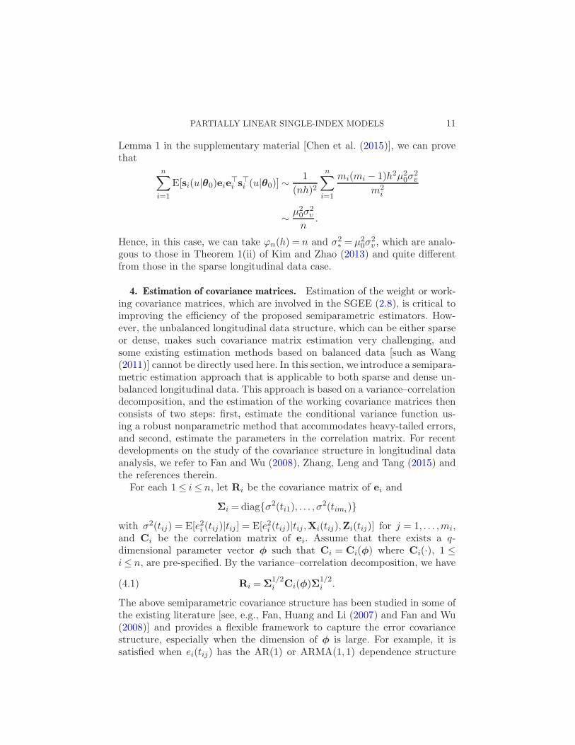
4. Estimation of covariance matrices. Estimation of the weight or work-ing covariance matrices, which are involved in the SGEE (2.8), is critical toimproving the efficiency of the proposed semiparametric estimators. How-ever, the unbalanced longitudinal data structure, which can be either sparseor dense, makes such covariance matrix estimation very challenging, andsome existing estimation methods based on balanced data [such as Wang(2011)] cannot be directly used here. In this section, we introduce a semipara-metric estimation approach that is applicable to both sparse and dense un-balanced longitudinal data. This approach is based on a variance–correlationdecomposition, and the estimation of the working covariance matrices thenconsists of two steps: first, estimate the conditional variance function us-ing a robust nonparametric method that accommodates heavy-tailed errors,and second, estimate the parameters in the correlation matrix. For recentdevelopments on the study of the covariance structure in longitudinal dataanalysis, we refer to Fan and Wu (2008), Zhang, Leng and Tang (2015) andthe references therein.

For each 1≤ i≤ n, let Ri be the covariance matrix of ei and

Σi = diagσ2(ti1), . . . , σ2(timi

)

with σ2(tij) = E[e2i (tij)|tij ] = E[e2i (tij)|tij ,Xi(tij),Zi(tij)] for j = 1, . . . ,mi,and Ci be the correlation matrix of ei. Assume that there exists a q-dimensional parameter vector φ such that Ci = Ci(φ) where Ci(·), 1 ≤i≤ n, are pre-specified. By the variance–correlation decomposition, we have

Ri =Σ1/2i Ci(φ)Σ

1/2i .(4.1)

The above semiparametric covariance structure has been studied in some ofthe existing literature [see, e.g., Fan, Huang and Li (2007) and Fan and Wu(2008)] and provides a flexible framework to capture the error covariancestructure, especially when the dimension of φ is large. For example, it issatisfied when ei(tij) has the AR(1) or ARMA(1,1) dependence structure


for each i; see, for example, the simulated example in Section 5.1. When

ei(tij) = σ(tij)(vi + εij) in which vi and εij satisfy the conditions discussedin Remark 3 and σ2

ε + σ2v = 1, we can also show that the semiparametric

covariance structure is satisfied with φ being σ2ε or σ2

v . Some existing pa-pers such as Wu and Pourahmadi (2003) suggest the use of a nonparametricsmoothing method to estimate the covariance matrix. However, they usuallyneed to assume that the longitudinal data are balanced or nearly balanced,which would be violated when the data are collected at irregular and possi-bly subject-specific time points. Yao, Muller and Wang (2005) proposed theapproach of functional data analysis to estimate the covariance structurefor sparse and irregularly-spaced longitudinal data. However, some substan-tial modification may be needed to extend the method of Yao, Muller andWang (2005) to our framework, which includes both the sparse and denselongitudinal data.

In the present paper, we first estimate the conditional variance functionσ2(·) in the diagonal matrix Σi by using a nonparametric method. In recentyears, there has been a rich literature on the study of nonparametric con-ditional variance estimation; see, for example, Fan and Yao (1998), Yu andJones (2004), Fan, Huang and Li (2007) and Leng and Tang (2011). However,when the errors are heavy-tailed, which is not uncommon in economic andfinancial data analysis, most of these existing methods may not performwell. This motivates us to devise an estimation method that is robust toheavy-tailed errors. Let r(tij) = [Yij −Z

⊤ijβ0 − η(X⊤

ijθ0)]2. We can then find

a random variable ξ(tij) so that r(tij) = σ2(tij)ξ2(tij) and E[ξ2(tij)|tij ] = 1

with probability one. By applying the log-transformation [see Peng and Yao(2003) and Chen, Cheng and Peng (2009) for the application of this trans-formation in time series analysis] to r(tij), we have

log r(tij) = log[τσ2(tij)] + log[τ−1ξ2(tij)]≡ σ2⋄(tij) + ξ⋄(tij),(4.2)

where τ is a positive constant such that E[ξ⋄(tij)] = Elog[τ−1ξ2(tij)]= 0.Here, ξ⋄(tij) could be viewed as an error term in model (4.2). As rij ≡ r(tij)are unobservable, we replace them with

rij = [Yij −Z⊤ijβ− η(X⊤

ij θ|β, θ)]2,

where β and θ are the PULS estimators of β0 and θ0, respectively. In orderto estimate σ2

⋄(t), we define

Ln(a, b) =

n∑

i=1

wi

h1

mi∑

j=1

[log(rij + ζn)− a− b(tij − t)]2K1

(tij − t

h1

),(4.3)

where K1(·) is a kernel function, h1 is a bandwidth satisfying Assumption 9in Appendix A, wi = 1/(nmi) as in Section 2 and ζn → 0 as n→∞. Through-out this paper, we set ζn = 1/Tn, where Tn =

∑ni=1mi. The ζn is added in


log(rij + ζn) to avoid the occurrence of invalid log 0 as ζn > 0 for any n.Such a modification would not affect the asymptotic distribution of the con-ditional variance estimation under certain mild restrictions. Then σ2

⋄(t) canbe estimated as

σ2⋄(t) = a where (a, b)⊤ = argmin

a,bLn(a, b).(4.4)

On the other hand, noting thatexpσ2

⋄(tij )τ ξ2(tij) = rij and E[ξ2(tij)] = 1,

the constant τ can be estimated by

τ =

[1

Tn

n∑

i=1

mi∑

j=1

rij exp−σ2⋄(tij)

]−1

.(4.5)

We then estimate σ2(t) by

σ2(t) =expσ2

⋄(t)

τ.(4.6)

It is easy to see that thus defined estimator σ2(t) is always positive.Suppose that there exists a sequence ϕn⋄(h1) which depends on h1, and

a constant 0< σ2⋄ <∞ such that

ϕn⋄(h1) = o(ωn),(4.7)

ϕn⋄(h1)

h21max1≤i≤n

w2iE

[mi∑

j=1

ξ⋄(tij)K1

(tij − t

h1

)]2= o(1)

and

ϕn⋄(h1)

fT (t)h21E

[n∑

i=1

wi

mi∑

j=1

ξ⋄(tij)K1

(tij − t

h1

)]2→ σ2

⋄ ,(4.8)

which are similar to those in (3.5) and (3.6), where fT (·) is the densityfunction of the observation times tij . Define

bσ1(t) =expσ2

⋄(t)

2τσ2⋄(t)

∫v2K1(v)dv,

bσ2(t) =expσ2

⋄(t)

2τE[σ2

⋄(tij)]

∫v2K1(v)dv,

where σ2⋄(·) is the second-order derivative of σ2

⋄(·). We then establish theasymptotic distribution of σ2(t) in the following theorem, whose proof isgiven in the supplementary material [Chen et al. (2015)].


Theorem 3. Suppose the conditions in Theorems 1 and 2, Assump-tions 6–9 in Appendix A, (4.7) and (4.8) are satisfied. Then we have

ϕ1/2n⋄ (h1)σ

2(t)− σ2(t)− [bσ1(t)− bσ2(t)]h21

d−→N

(0,

σ4(t)

fT (t)σ2⋄

).(4.9)

Remark 4. Theorem 3 can be seen as an extension of Theorem 1 inChen, Cheng and Peng (2009) from the time series case to the longitudinaldata case. The longitudinal data framework in this paper is more flexibleand includes both sparse and dense data types. If ξ⋄(tij) = v⋄i +ε⋄ij , where ε

⋄ij

are i.i.d. across both i and j with E[ε⋄ij ] = 0 and E[(ε⋄ij)2]<∞, and v⋄i is

an i.i.d. sequence of random variables with E[v⋄i ] = 0 and E[(v⋄i )2]<∞ and

is independent of ε⋄ij, following the discussion in Remark 3, we can again

show that the form of ϕn⋄(h1) depends on the type of the longitudinal data,and thus the nonparametric conditional variance estimation has differentconvergence rates for sparse and dense data.

We next discuss how to obtain the optimal value of the parameter vec-

tor φ. Construct the residuals ei =Yi − Ziβ − η(Xi, θ), where η(Xi, θ) isdefined in the same way as η(Xi,θ) but with η(·) and θ replaced by η(·)≡

η(·|β, θ) and θ, respectively. Let Λi ≡ Λi(θ), Σi = diagσ2(ti1), . . . , σ2(timi

),

and define R∗i (φ) = Σ

1/2

i Ci(φ)Σ1/2

i . Motivated by equations (3.1) and (3.2),we construct

Ω∗0(φ) =

n∑

i=1

Λ⊤

i [R∗i (φ)]

−1Λi(4.10)

and

Ω∗1(φ) =

n∑

i=1

Λ⊤

i [R∗i (φ)]

−1eie

⊤i [R

∗i (φ)]

−1Λi.(4.11)

By Theorem 1, the sandwich formula estimate [Ω∗0(φ)]

+Ω

∗1(φ)[Ω

∗0(φ)]

+ isasymptotically proportional to the asymptotic covariance of the proposedSGEE estimators when the inverse of R∗

i (φ) is chosen as the weight matrix.

The optimal value of φ, denoted by φ, can be chosen to minimize the de-terminant |[Ω∗

0(φ)]+Ω

∗1(φ)[Ω

∗0(φ)]

+|. Such a method is called the minimumgeneralized variance method [Fan, Huang and Li (2007)]. With the chosen

φ, we can estimate the covariance matrices by

Ri(φ) = Σ1/2

i Ci(φ)Σ1/2

i ,(4.12)

whose inverse will be used as the weight matrices in the SGEE method.


5. Numerical studies. In this section, we first study the finite sampleperformance of the proposed SGEE estimators through Monte Carlo sim-ulation, and then give an empirical application of the proposed model andmethodology.

5.1. Simulation studies. We investigate both sparse and dense longitu-dinal data cases with an average time dimension m of 10 for the sparsedata and 30 for the dense data. We use two types of within-subject cor-relation structure, AR(1) and ARMA(1,1), in the error terms ei(tij). Weinvestigate the finite sample performance of the proposed estimators underboth correct specification and misspecification of the correlation structure inthe construction of the covariance matrix estimator proposed in Section 4.For the misspecified case, we fit an AR(1) correlation structure while thetrue underlying structure is ARMA(1,1) and examine the robustness of theestimators.

Simulated data are generated from model (1.2) with two-dimensionalZi(tij) and three-dimensional Xi(tij), and

β0 = (2,1)⊤, θ0 = (2,1,2)⊤/3 and η(u) = 0.5exp(u).

The covariates (Z⊤i (tij),X

⊤i (tij))

⊤ are generated independently from a five-dimensional Gaussian distribution with mean 0, variance 1 and pairwisecorrelation 0.1. The observation times tij are generated in the same wayas in Fan, Huang and Li (2007): for each subject, 0,1,2, . . . , T is a set ofscheduled times, and each scheduled time from 1 to T has a 0.2 probabilityof being skipped; each actual observation time is a perturbation of a non-skipped scheduled time; that is, a uniform [0,1] random number is added tothe nonskipped scheduled time. Here T is set to be 12 or 36, which corre-sponds to an average time dimension of m= 10 or m= 30, respectively. Foreach i, the error terms ei(tij) are generated from a Gaussian process withmean 0, variance function

var[e(t)] = σ2(t) = 0.25exp(t/12)(5.1)

and serial correlation structure

cor(e(t), e(s)) =

1, t= s,

γρ|t−s|, t 6= s.(5.2)

Note that (5.2) corresponds to an ARMA(1,1) correlation structure andreduces to an AR(1) correlation structure when γ = 1. The number of sub-jects, n, is taken to be 30 or 50. The values for γ and ρ are (γ, ρ) = (0.85,0.9)in the ARMA(1,1) correlation structure and (γ, ρ) = (1,0.9) in the AR(1)structure.

For each combination of m, n, and the correlation structure, the numberof simulation replications is 200. For the selection of the bandwidth, however,


Table 1

Performance of parameter estimation methods under correct specification of anunderlying AR(1) correlation structure

n 30 50

m Parameters Methods Bias SD MAD Bias SD MAD

10 β1 PULS 0.0048 0.0402 0.0288 −0.0030 0.0308 0.0195SGEE −0.0026 0.0508 0.0081 −0.0016 0.0259 0.0074

β2 PULS −0.0024 0.0409 0.0243 0.0049 0.0267 0.0180SGEE −0.0018 0.0298 0.0110 0.0033 0.0310 0.0077

θ1 PULS −0.0049 0.0299 0.0180 −0.0009 0.0197 0.0134SGEE −0.0013 0.0164 0.0083 −0.0002 0.0118 0.0046

θ2 PULS 0.0011 0.0380 0.0229 −0.0016 0.0237 0.0161SGEE 0.0026 0.0188 0.0100 0.0006 0.0108 0.0067

θ3 PULS 0.0018 0.0314 0.0188 0.0006 0.0203 0.0147SGEE −0.0007 0.0182 0.0090 −0.0004 0.0088 0.0052

30 β1 PULS 0.0003 0.0408 0.0277 0.0016 0.0328 0.0222SGEE −0.0081 0.1134 0.0106 0.0007 0.0108 0.0083

β2 PULS −0.0020 0.0425 0.0317 0.0005 0.0351 0.0202SGEE −0.0017 0.0420 0.0096 −0.0064 0.0152 0.0079

θ1 PULS 0.0020 0.0315 0.0213 −0.0020 0.0244 0.0182

SGEE −0.0008 0.0247 0.0075 0.0001 0.0148 0.0064

θ2 PULS −0.0035 0.0340 0.0240 −0.0083 0.0278 0.0163SGEE −0.0027 0.0242 0.0090 −0.0013 0.0104 0.0066

θ3 PULS −0.0027 0.0321 0.0185 0.0045 0.0267 0.0169SGEE 0.0009 0.0230 0.0074 0.0001 0.0162 0.0068

due to the running time limitation, we first run a leave-one-unit-out (i.e.,leave out observations from one subject at a time) cross-validation (CV) tochoose the optimal bandwidths from 20 replications. We then use the aver-age of the optimal bandwidths from these 20 replications as the bandwidthin the 200 replications of the simulation study. For the SGEE method, wechoose the weight matrix as the inverse of the estimated within-subject co-variance matrix as constructed in (4.12) of Section 4. We first study theperformance of the proposed estimators in the case where the correlationstructure in the estimation of the covariance matrix is correctly specified,and then investigate the robustness of the estimators to the misspecifica-tion of the correlation structure. The bias, calculated as the average of theestimates from the 200 replications minus the true parameter values, thestandard deviation (SD), calculated as the sample standard deviation of the200 estimates and the median absolute deviation (MAD), calculated as themedian absolute deviation of the 200 estimates are reported in Tables 1


Table 2

Performance of parameter estimation methods under correct specification of anunderlying ARMA(1,1) correlation structure

n 30 50


10 β1 PULS −0.0029 0.0400 0.0280 0.0006 0.0322 0.0221SGEE −0.0025 0.0244 0.0155 0.0000 0.0193 0.0124

β2 PULS 0.0032 0.0386 0.0282 −0.0045 0.0299 0.0205SGEE 0.0009 0.0249 0.0171 0.0001 0.0212 0.0126

θ1 PULS −0.0004 0.0267 0.0181 −0.0003 0.0188 0.0126SGEE −0.0002 0.0161 0.0104 0.0006 0.0146 0.0073

θ2 PULS −0.0047 0.0343 0.0209 0.0005 0.0223 0.0156SGEE −0.0031 0.0192 0.0113 −0.0002 0.0145 0.0087

θ3 PULS 0.0008 0.0253 0.0158 −0.0009 0.0201 0.0121SGEE 0.0011 0.0148 0.0102 −0.0009 0.0146 0.0074

30 β1 PULS −0.0026 0.0450 0.0296 −0.0016 0.0374 0.0273SGEE 0.0005 0.0214 0.0138 0.0015 0.0288 0.0105

β2 PULS −0.0013 0.0461 0.0291 0.0035 0.0361 0.0252SGEE 0.0040 0.0335 0.0147 0.0014 0.0152 0.0104

θ1 PULS −0.0014 0.0296 0.0192 −0.0010 0.0207 0.0159SGEE −0.0005 0.0166 0.0095 0.0006 0.0092 0.0063

θ2 PULS −0.0050 0.0355 0.0231 0.0011 0.0229 0.0173SGEE −0.0037 0.0371 0.0120 −0.0003 0.0116 0.0072

θ3 PULS 0.0017 0.0279 0.0186 −0.0006 0.0215 0.0154SGEE 0.0009 0.0181 0.0095 −0.0007 0.0100 0.0070

and 2. Table 1 gives the results obtained under the correct specification ofan underlying within-subject AR(1) correlation structure in ei(tij), and Ta-ble 2 gives those obtained under the correct specification of an underlyingARMA(1,1) structure in ei(tij). For comparison, we also report the resultsfrom the PULS estimation. The results in Tables 1 and 2 show that theSGEE estimates are comparable with the PULS estimates in terms of biasand are more efficient than the PULS estimates, which supports the asymp-totic theory developed in Section 3. In Figures 1 and 2, we plot the locallinear estimated link function from a typical realization together with thereal curve for each combination of n and m.

To investigate the robustness of the SGEE and PULS estimators to cor-relation structure misspecification, we also carry out a simulation study inwhich an AR(1) correlation structure is used in the covariance matrix esti-mation detailed in Section 4, when the true underlying correlation structureis ARMA(1,1). Table 3 reports the results under this misspecification. The


(a) (b)

(c) (d)

Fig. 1. Estimated link function (dot-dashed line), together with the true link function(solid line), from a typical realization of model (1.2) with AR(1) correlation structure foreach combination of n and m: (a) n= 30, m= 10; (b) n= 50, m= 10; (c) n= 30, m= 30;(d) n= 50, m= 30.

table shows that in the presence of correlation structure misspecification,SGEE still produces more efficient parameter estimates than PULS.

We also include a simulated example where the covariates in Z followdiscrete distributions. The same model as above is used except that thecovariates X⊤

i (tij) are drawn independently from a three-dimensional Gaus-sian distribution with mean 0, variance 1 and pairwise correlation 0.1, andZ⊤i (tij) are independently drawn from a binomial distribution with success

probability 0.5. The errors ei(tij) are generated with the AR(1) serial corre-lation structure of (γ, ρ) = (1,0.9). The simulation results for this exampleare presented in Table 4. The same finding as above can be obtained. Someadditional results, that is, those on the average angles between the estimatedand the true parameter vectors, are given in Appendix D of the supplemen-tary material [Chen et al. (2015)].

5.2. Real data analysis. We next illustrate the partially linear single-index model and the proposed SGEE estimation method through an empir-ical example which explores the relationship between lung function and air


(a) (b)

(c) (d)

Fig. 2. Estimated link function (dot-dashed line), together with the true link function(solid line), from a typical realization of model (1.2) with ARMA(1,1) correlation structurefor each combination of n and m: (a) n = 30, m = 10; (b) n = 50, m = 10; (c) n = 30,m= 30; (d) n= 50, m= 30.

pollution. There is voluminous literature studying the effects of air pollu-tion on people’s health. For a review of the literature, the reader is referredto Pope, Bates and Raizenne (1995). Many studies have found associationbetween air pollution and health problems such as increased respiratorysymptoms, decreased lung function, increased hospitalizations or hospitalvisits for respiratory and cardiovascular diseases and increased respiratorymorbidity [Dockery et al. (1989), Kinney et al. (1989), Pope (1991), Braun-Fahrlander et al. (1992), Lipfert and Hammerstrom (1992)]. While earlierresearch often used time series or cross-sectional data to evaluate the healtheffects of air pollution, recent advances in longitudinal data analysis tech-niques offer greater opportunities for studying this problem. In this paper,we will examine whether air pollution has a significant adverse effect onlung function, and, if so, to what extent. The use of the partially linearsingle-index model and the SGEE method would provide greater modelingflexibility than linear models and allow the within-subject correlation to beadequately taken into account. We will use a longitudinal data set obtainedfrom a study where a total of 971 4th-grade children aged between 8 and 14


Table 3

Performance of parameter estimation methods under misspecification of an underlyingARMA(1,1) correlation structure

n 30 50


10 β1 PULS 0.0072 0.0410 0.0357 −0.0038 0.0299 0.0201SGEE −0.0054 0.0261 0.0210 −0.0055 0.0211 0.0147

β2 PULS 0.0068 0.0336 0.0256 0.0037 0.0290 0.0163SGEE 0.0025 0.0267 0.0157 0.0023 0.0190 0.0136

θ1 PULS 0.0037 0.0166 0.0114 0.0061 0.0157 0.0096SGEE 0.0033 0.0144 0.0122 0.0016 0.0163 0.0081

θ2 PULS −0.0092 0.0303 0.0184 −0.0084 0.0224 0.0174SGEE −0.0007 0.0198 0.0144 −0.0045 0.0203 0.0130

θ3 PULS −0.0005 0.0229 0.0158 −0.0028 0.0160 0.0111SGEE −0.0035 0.0141 0.0094 0.0000 0.0134 0.0092

30 β1 PULS 0.0066 0.0403 0.0259 −0.0221 0.0502 0.0252SGEE 0.0093 0.0144 0.0087 0.0001 0.0165 0.0118

β2 PULS −0.0138 0.0435 0.0353 0.0107 0.0312 0.0233SGEE −0.0017 0.0268 0.0096 0.0035 0.0170 0.0096

θ1 PULS 0.0027 0.0252 0.0165 0.0020 0.0181 0.0067SGEE 0.0054 0.0136 0.0078 0.0019 0.0096 0.0098

θ2 PULS −0.0063 0.0265 0.0245 0.0021 0.0315 0.0273SGEE 0.0009 0.0198 0.0118 0.0046 0.0136 0.0094

θ3 PULS −0.0011 0.0285 0.0258 −0.0042 0.0217 0.0136SGEE −0.0065 0.0178 0.0137 −0.0046 0.0120 0.0084

years (at their first visit to the hospital/clinic) were followed over 10 years.For each yearly visit of the children to the hospital/clinic, records on theirforced expiratory volume (FEV), asthma symptom at visit (ASSPM, 1 forthose with symptoms and 0 for those without), asthmatic status (ASS, 1 forasthma patient and 0 for nonasthma patient), gender (G, 1 for males and0 for females), race (R, 1 for nonwhites and 0 for whites), age (A), height(H), BMI and respiratory infection at visit (RINF, 1 for those with infectionand 0 for those without) were taken. Together with the measurements fromthe children, the mean levels of ozone and NO2 in the month prior to thevisit were also recorded. Due to dropout or other reasons, the majority ofchildren had 4 to 5 years of records, and the total number of observationsin the data set is 3809.

As in many other studies, the FEV will be used as a measure of lungfunction, and its log-transformed values, log(FEV), will be used as the re-sponse values in our model. Our main interest is to determine whether higher


Table 4

Performance of parameter estimation methods under correct specification of anunderlying AR(1) correlation structure when the covariates in Z are discrete

n 30 50


10 β1 PULS 0.0215 0.0530 0.0404 0.0018 0.0646 0.0472SGEE 0.0228 0.0511 0.0208 0.0037 0.0298 0.0138

β2 PULS −0.0309 0.0858 0.0735 0.0193 0.0526 0.0498SGEE 0.0024 0.0313 0.0193 0.0074 0.0339 0.0274

θ1 PULS −0.0012 0.0185 0.0090 −0.0116 0.0201 0.0175SGEE −0.0060 0.0157 0.0082 0.0020 0.0086 0.0066

θ2 PULS −0.0020 0.0263 0.0232 0.0138 0.0229 0.0172SGEE 0.0122 0.0241 0.0143 −0.0004 0.0087 0.0063

θ3 PULS 0.0012 0.0206 0.0075 0.0036 0.0153 0.0132SGEE −0.0008 0.0078 0.0048 −0.0020 0.0070 0.0034

30 β1 PULS 0.0075 0.0427 0.0222 0.0108 0.0723 0.0513SGEE 0.0061 0.0284 0.0233 0.0033 0.0226 0.0175

β2 PULS −0.0143 0.0768 0.0401 0.0023 0.0681 0.0417SGEE 0.0116 0.0275 0.0125 −0.0039 0.0259 0.0196

θ1 PULS −0.0159 0.0310 0.0252 0.0031 0.0218 0.0168SGEE −0.0030 0.0083 0.0045 0.0015 0.0098 0.0064

θ2 PULS −0.0026 0.0192 0.0112 0.0048 0.0252 0.0200SGEE 0.0040 0.0200 0.0133 0.0002 0.0115 0.0084

θ3 PULS 0.0151 0.0331 0.0308 −0.0067 0.0228 0.0150SGEE 0.0006 0.0133 0.0083 −0.0018 0.0103 0.0064

levels of ozone and NO2 would lead to decrements in lung function. Toaccount for the effects of other confounding factors, we include all otherrecorded variables. As age and height exhibit strong co-linearity (with acorrelation of 0.78), we will only use height in the study. In fitting the par-tially linear single-index model to the data, all the continuous variables (i.e.,FEV, H, BMI, OZONE and NO2) are log-transformed, and the log(BMI),log(OZONE) and log(NO2) are included in the single-index part. The log(H)and all the binary variables are included in the linear part of the model.

The scatter plots of the response variable against the continuous regres-sors are shown in Figure 3, and the box plots of the response against thebinary regressors are given in Figure 4. We use an ARMA(1,1) within-subject correlation structure in the estimation of the covariance matrix forthe proposed SGEE method. The resulting estimated model is as follows:

log(FEV)

≈ 0.0325 ∗G− 0.0111 ∗ASS− 0.0671 ∗R


Fig. 3. The scatter plots of the response variable log(FEV) against the continuous re-gressors, that is, (clockwise from top left) log(H), log(BMI), log(NO2), log(OZONE).

(0.0041) (0.0080) (0.0059)

− 0.0047 ∗ASSPM− 0.0068 ∗RINF+ 2.3206 ∗ log(H),

(0.0085) (0.0043) (0.0307)

+ η[0.9929 ∗ log(BMI)− 0.0924 ∗ log(OZONE)− 0.0753 ∗ log(NO2)]

(0.0560) (0.0127) (0.0125),

where the numbers in the parentheses under the estimated coefficien’s aretheir respective estimated standard errors. The estimated link function andits 95% point-wise confidence intervals are plotted in Figure 5.

From Figure 5, it can be seen that the estimated link function is overallincreasing. The 95% point-wise confidence intervals show that a linear func-tional form for the unknown link function would be rejected, and thus thepartially liner single-index model might be more appropriate than the tra-ditional linear regression model. Meanwhile, it can be seen from the aboveestimated model that height and BMI are significant positive factors in ac-counting for lung function. Taller children and children with larger BMI tendto have higher FEV. Furthermore, male and white children have, on average,higher FEV than female or nonwhite children. Furthermore, both OZONEand NO2 in the single-index component have negative effects on children’s


Fig. 4. The box plots of the response variable log(FEV) against the binary regressors,that is, (clockwise from top left) G, ASS, R, RINF, ASSPM.

lung function, as the estimated coefficients for OZONE and NO2 are nega-tive, and the estimated link function is increasing. Although these negativeeffects are relatively small in magnitude compared to the effect of BMI, theyare statistically significant. This means that higher levels of ozone and NO2

tend to lead to reduced lung function as represented by lower values of FEV.

6. Conclusions and discussions. In this paper, we study a partially linearsingle-index modeling structure for possibly unbalanced longitudinal data in

Fig. 5. The estimated link function and its 95% point-wise confidence intervals.


a general framework, which includes both the sparse and dense longitudinaldata cases. An SGEE method with the first-stage local linear smoothing isintroduced to estimate the two parameter vectors as well as the unspecifiedlink function.

In Theorems 1 and 2, we derive the asymptotic properties of the pro-posed parametric and nonparametric estimators in different scenarios, fromwhich we find that the convergence rates and asymptotic variances of theresulting estimators in the sparse longitudinal data case could be substan-tially different from those in the dense longitudinal data. In Section 4, wepropose a semiparametric method to estimate the error covariance matriceswhich are involved in the estimation equations. The conditional variancefunction is estimated by using the log-transformed local linear method, andthe parameters in the correlation matrices are estimated by the minimumgeneralized variance method. In particular, if the correlation matrices arecorrectly specified, as is stated in Corollary 1, the SGEE-based estimatorsβ and θ are generally asymptotically more efficient than the correspond-

ing PULS estimators β and θ in the sense that the asymptotic covariancematrix of the SGEE estimators minus that of the PULS estimators is nega-tive semi-definite. Both the simulation study and empirical data analysis inSection 5 show that the proposed methods work well in the finite samples.

Recently, Yao and Li (2013) developed a new nonparametric regressionfunction estimation method for a longitudinal regression model. This methodtakes into account the within-subject correlation information and thus gen-erally improves the asymptotic estimation efficiency. It would also be inter-esting to incorporate the within-subject correlation information in the locallinear estimation of the unknown link function in this paper and to examineboth theoretical and empirical performance of the resulting estimator. Wewill leave this issue for future research. Another possible future topic is toextend the semiparametric techniques of variable selection and specificationtesting proposed by Liang et al. (2010) from the i.i.d. case to the generallongitudinal data case discussed in the present paper.

APPENDIX A: REGULARITY CONDITIONS

To establish the asymptotic properties of the SGEE estimators proposedin Section 2, we introduce the following regularity conditions, although someof them might not be the weakest possible.

Assumption 1. The kernel function K(·) is a bounded and symmetricprobability density function with compact support. Furthermore, the kernelfunction has a continuous first-order derivative function denoted by K(·).


Assumption 2. (i) The errors eij ≡ ei(tij), 1 ≤ i ≤ n, 1 ≤ j ≤mi, areindependent across i; that is, ei defined in Section 2, 1≤ i≤ n, are mutuallyindependent.

(ii) The covariates Xij and Zij , 1 ≤ i ≤ n, 1 ≤ j ≤mi, are i.i.d. randomvectors.

(iii) The errors eij are independent of the covariates Zij and Xij , andfor each i, eij , 1≤ j ≤mi, may be correlated with each other. Furthermore,E[eij ] = 0, 0 < E[e2ij ] <∞ and E[|eij |

2+δ ] <∞ for some δ > 0. The largest

eigenvalues of Wi and WiE[eiei]Wi are bounded for any i.

Assumption 3. (i) The density function fθ(·) of X⊤ijθ is positive and

has a continuous second-order derivative in U = x⊤θ :x ∈X ,θ ∈Θ, whereΘ is a compact parameter space for θ and X is a compact support of Xij .

(ii) The function ρZ(u|θ) = E[Zij |X⊤ijθ = u] has a bounded and continuous

second-order derivative (with respect to u) for any θ ∈Θ, and E[‖Zij‖2+δ]<

∞, where δ was defined in Assumption 2(iii).

Assumption 4. The link function η(·) has continuous derivatives up tothe second order.

Assumption 5. The bandwidth h satisfies

ωnh6 → 0,

n2h2

Nn(h) logn→∞,

T2/(2+δ)n logn

h2Nn(h)= o(1),(A.1)

where Nn(h) =∑n

i=1 1/(mih), Tn =∑n

i=1mi and δ was defined in Assump-

tion 2(iii). Furthermore, max1≤i≤n(m4i +m3

ih−1) = o(wn).

Remark 5. Assumption 1 imposes some mild restrictions on the kernelfunctions, which have been used in the existing literature in i.i.d. and weaklydependent time series cases; see, for example, Fan and Gijbels (1996) andGao (2007). The compact support restriction on the kernel functions can beremoved if we impose certain restrictions on the tail of the kernel function.In Assumption 2(i), the longitudinal data under investigation is assumed tobe independent across subjects i, which is not uncommon in longitudinaldata analysis; see, for example, Wu and Zhang (2006) and Zhang, Fan andSun (2009). Assumption 2(ii) is imposed to simplify the presentation ofthe asymptotic results. However, we may replace Assumption 2(ii) with theconditions that the covariates Xij and Zij are i.i.d. across i and identicallydistributed across j, and in the case of dense longitudinal data, it is furthersatisfied that for κ= 0,1,2, . . . ,

Var

[1

mi

mi∑

j=1

Uij

h

(X

⊤ijθ− u

h

)κ

K

(X

⊤ijθ− u

h

)]≤C(mih)

−1(A.2)


uniformly for u ∈ U and θ ∈Θ, where Uij can be 1, ZijB1(Zij), orXijB2(Xij),B1(·) and B2(·) are two bounded functions, and C is a positive constantwhich is independent of i. When Xij and Zij are stationary and α-mixingdependent across j for the case of dense longitudinal data, it is easy to vali-date the high-level condition (A.2). In Assumption 2(iii), we allow the errorterms to have certain within-subject correlation, which makes the modelassumptions more realistic. Assumption 3 gives some commonly-used condi-tions in partially linear single-index models; see Xia and Hardle (2006) andChen, Gao and Li (2013b), for example. Assumption 4 is a mild smoothnesscondition on the link function imposed for the application of the local linearfitting. Assumption 5 gives a set of restrictions on the bandwidth h, whichis involved in the estimation of the link function. Note that the bandwidthconditions in Assumption 5 imply that the milder bandwidth conditions in(C.1) of Lemma 1 in the supplemental material [Chen et al. (2015)] aresatisfied. Hence we can use Lemma 1 to prove our main theoretical results.

We next give some regularity conditions, which are needed to derive theasymptotic property of the nonparametric conditional variance estimatorsin Section 4.

Assumption 6. The kernel function K1(·) is a continuous and symmet-ric probability density function with compact support.

Assumption 7. The observation times, tij , are i.i.d. and have a contin-uous and positive probability density function fT (t), which has a compactsupport T . The density function of ξ2(tij) is continuous and bounded. Letδ > 2, which strengthens the moment conditions in Assumptions 2 and 3.

Assumption 8. The conditional variance function σ2(·) has a continu-ous second-order derivative and satisfies inft∈T σ2(t)> 0. Let σ2(·) and σ2(·)be its first-order and second-order derivative functions, respectively.

Assumption 9. The bandwidth h1 satisfies

h1 → 0,T2/(2+δ/2)n logn

h21Nn(h1)= o(1),(A.3)

where Nn(h1) =∑n

i=1 1/(mih1).

Remark 6. Assumption 7 imposes a mild condition on the observationtimes [see, e.g., Jiang and Wang (2011)] and strengthens the moment condi-tions on eij and Zij . However, such moment conditions are not uncommonin the asymptotic theory for nonparametric conditional variance estimation


[Chen, Cheng and Peng (2009)]. Since the local linear smoothing techniqueis applied, a certain smoothness condition has to be assumed on σ2(·), asis done in Assumption 8. Assumption 9 gives some mild restrictions on thebandwidth h1, which is used in the estimation of the conditional variancefunction.

APPENDIX B: PROOFS OF THE MAIN RESULTS

In this appendix, we provide the detailed proofs of the main results givenin Section 3.

B.1. Proof of Theorem 1. By the definition of the weighted local linearestimators in (2.4) and (2.5), we have

η(u|β,θ)− η(u) =

n∑

i=1

si(u|θ)(Yi −Ziβ)− η(u)

=

n∑

i=1

si(u|θ)ei +

n∑

i=1

si(u|θ)Zi(β0 −β)

+n∑

i=1

si(u|θ)[η(Xi,θ0)− η(Xi,θ)](B.1)

+

n∑

i=1

si(u|θ)η(Xi,θ)− η(u)

≡ In1 + In2 + In3 + In4.

For In1, note that by a first-order Taylor expansion of K(·), we have, fori= 1, . . . , n and j = 1, . . . ,mi,

K

(X

⊤ijθ− u

h

)=K

(X

⊤ijθ0 − u

h

)+ K

(X

⊤ijθ∗ − u

h

)X

⊤ij(θ− θ0)

h,

where K(·) is the first-order derivative of K(·) and θ∗ = θ0 + λ∗(θ − θ0),0< λ∗ < 1. Hence, by some standard calculations and the assumption thatn2h2/Nn(h) logn→∞, we have

In1 =

n∑

i=1

si(u|θ0)ei +

n∑

i=1

[si(u|θ)− si(u|θ0)]ei

=n∑

i=1

si(u|θ0)ei +OP

(‖θ− θ0‖ ·

√Nn(h) logn

nh

)(B.2)


=

n∑

i=1

si(u|θ0)ei + oP (‖θ− θ0‖)

for any u ∈ U and θ ∈Θ.By Lemma 2 in the supplementary material [Chen et al. (2015)], we can

prove that

In2 =−ρ⊤Z(u)(β− β0) +OP (‖β− β0‖2 + ‖θ− θ0‖

2)(B.3)

for any u ∈ U , where ρZ(u)≡ ρZ(u|θ0) = E[Zij|X⊤ijθ0 = u].

Note that

η(X⊤ijθ)− η(X⊤

ijθ0) = η(X⊤ijθ0)X

⊤ij(θ− θ0) +OP (‖θ− θ0‖

2),

which, together with Lemma 3 in the supplementary material [Chen et al.(2015)], leads to

In3 =−η(u)ρ⊤X(u)(θ − θ0) +OP (‖θ− θ0‖2)(B.4)

for any u ∈ U , where ρX(u)≡ ρX(u|θ0) = E[Xij|X⊤ijθ0 = u].

By a second-order Taylor expansion of η(·) and the first-order Taylorexpansion of K(·) used to handle In1, we can prove that, for any u ∈ U , wehave

In4 =12µ2η(u)h

2[1 +OP (h)] + oP (‖θ − θ0‖).(B.5)

Recall that β and θ1 are the solutions to the equations in (2.8). By (B.1)–(B.5), we can prove that, uniformly for i= 1, . . . , n and j = 1, . . . ,mi,

η(X⊤ij θ1|β, θ1)− η(X⊤

ijθ0)

= η(X⊤ij θ1|β, θ1)− η(X⊤

ijθ0|β, θ1) + η(X⊤ijθ0|β, θ1)− η(X⊤

ijθ0)

= η(X⊤ijθ0|β, θ1)X

⊤ij(θ1 − θ0) + η(X⊤

ijθ0|β, θ1)− η(X⊤ijθ0)

+OP (‖θ1 − θ0‖2)(B.6)

= η(X⊤ijθ0)[Xij − ρX(X

⊤ijθ0)]

⊤(θ1 − θ0)(1 + oP (1))

+

n∑

k=1

sk(X⊤ijθ0)ek − ρ⊤Z(X

⊤ijθ0)(β−β0)(1 + oP (1))

+ 12µ2η(X

⊤ijθ0)h

2 +OP (h3) +OP (‖θ1 − θ0‖

2 + ‖β−β0‖2),

where sk(X⊤ijθ0)≡ sk(X

⊤ijθ0|θ0).

By the definitions of β and θ1 [see (2.8) in Section 2], we have

n∑

i=1

Λ⊤

i (θ1)Wi[Yi −Ziβ− η(Xi|β, θ1)] = 0.(B.7)


By the uniform consistency results for the local linear estimators (such asLemmas 2 and 3 in the supplementary material [Chen et al. (2015)]), we can

approximate Λi(θ1) in (B.7) by Λi =Λi(θ0) when deriving the asymptoticdistribution theory. Then we have

0=

n∑

i=1

Λ⊤

i (θ1)Wi[Yi −Ziβ− η(Xi|β, θ1)]

=

n∑

i=1

Λ⊤i Wi[Yi −Ziβ− η(Xi|β, θ1)](B.8)

+

n∑

i=1

(Λi(θ1)−Λi)⊤Wi[Yi −Ziβ− η(Xi|β, θ1)]

P∼

n∑

i=1

Λ⊤i Wi[Yi −Ziβ− η(Xi|β, θ1)][1 +OP (‖θ1 − θ0‖)],

where and below anP∼ bn denotes an = bn(1+oP (1)). Furthermore, note that

Yi −Ziβ− η(Xi|β, θ1) = ei −Zi(β−β0)− [η(Xi|β, θ1)− η(Xi,θ0)],

which, together with (B.6) and the bandwidth condition ωnh6 = o(1), implies

thatn∑

i=1

Λ⊤i Wi[Yi −Ziβ− η(Xi|β, θ1)]

=

n∑

i=1

Λ⊤i Wiei −

n∑

i=1

Λ⊤i WiZi(β−β0)

−

n∑

i=1

Λ⊤i Wi[η(Xi|β, θ1)− η(Xi,θ0)]

=−n∑

i=1

Λ⊤i Wi[Zi − ρZ(Xi,θ0)](β−β0)(1 + oP (1))

(B.9)

−

n∑

i=1

Λ⊤i Wi[η(Xi,θ0)⊗ 1

⊤p ]⊙ [Xi − ρX(Xi,θ0)]

× (θ1 − θ0)(1 + oP (1))

+

n∑

i=1

Λ⊤i Wi

[ei −

n∑

k=1

sk(Xi,θ0)ek

]

+OP (‖β− β0‖2 + ‖θ1 − θ0‖

2),


where sk(Xi,θ0) = [s⊤k (X⊤i1θ0), . . . , s

⊤k (X

⊤imi

θ0)]⊤, ρZ(Xi,θ0) and ρX(Xi,θ0)

were defined in Section 2. Following the standard proof in the existing lit-erature [see, e.g., Ichimura (1993), Chen, Gao and Li (2013b)], we can show

the weak consistency of β and θ1. Note that

n∑

i=1

Λ⊤i WiΛi

(β− β0

θ1 − θ0

)

=n∑

i=1

Λ⊤i Wi[η(Xi,θ0)⊗ 1

⊤p ]⊙ [Xi − ρX(Xi,θ0)](θ1 − θ0)

+

n∑

i=1

Λ⊤i Wi[Zi − ρZ(Xi,θ0)](β −β0)

andn∑

i=1

Λ⊤i Wi

[n∑

k=1

sk(Xi,θ0)ek

]= oP (ω

1/2n ),

which, together with (B.8) and (B.9), lead to[

n∑

i=1

Λ⊤i WiΛi

](β−β0

θ1 − θ0

)P∼

n∑

i=1

Λ⊤i Wiei.(B.10)

Define I(θ0,B0) = diagId,M,O(θ0) =(Od×d Od×1

Op×d θ0

), whereM= (θ0,B0)

was defined in Section 3. It is easy to find that

Id+p = I(θ0,B0)I⊤(θ0,B0) =O(θ0)O

⊤(θ0) + I(B0)I⊤(B0).(B.11)

By the identification condition on θ0, we may show that

θ− θ0 =θ1

‖θ1‖−

θ0

‖θ0‖=

θ1

‖θ1‖−

θ0

‖θ1‖+

θ0

‖θ1‖−

θ0

‖θ0‖

P∼

θ1 − θ0

‖θ0‖− θ0θ

⊤0

θ1 − θ0

‖θ0‖= (Ip − θ0θ

⊤0 )(θ1 − θ0),

which implies that θ− θ0 =B0B⊤0 (θ1 − θ0) and

(β−β0

θ− θ0

)= I(B0)I

⊤(B0)

(β−β0

θ1 − θ0

).(B.12)

By (B.10), (B.11) and using the fact that ΛiO(θ0) = 0, we have

I⊤(B0)

[n∑

i=1

Λ⊤i WiΛi

]I(B0)I

⊤(B0)

(β− β0

θ1 − θ0

)P∼ I

⊤(B0)

[n∑

i=1

Λ⊤i Wiei

],


which, together with (B.12), implies that(β− β0

θ− θ0

)P∼ I(B0)

I⊤(B0)

[n∑

i=1

Λ⊤i WiΛi

]I(B0)

−1

I⊤(B0)

[n∑

i=1

Λ⊤i Wiei

].

Thus, by (3.1)–(3.3), the definition of the Moore–Penrose inverse and theclassical central limit theorem for independent sequence, we can show that(3.4) in Theorem 1 holds.

B.2. Proof of Corollary 1. By Theorem 1, the PULS estimators β andθ have the following asymptotic normal distribution:

ω1/2n

(β−β0

θ− θ0

)d

−→N(0,Ω+0∗Ω1∗Ω

+0∗),(B.13)

where Ω0∗ and Ω1∗ are two matrices such that

1

ωn

n∑

i=1

Λ⊤i Λi

P→Ω0∗,

1

ωn

n∑

i=1

E[Λ⊤i ViΛi]→Ω1∗,

and Vi is the conditional covariance matrix of ei.On the other hand, when the weights Wi, i= 1, . . . , n, are chosen as the

inverse of Vi, by Theorem 1, we have

ω1/2n

(β−β0

θ− θ0

)d

−→N(0,Ω+∗ ),(B.14)

where Ω∗ is a positive semi-definite matrix such that

1

ωn

n∑

i=1

E[Λ⊤i V

−1i Λi]→Ω∗.

In order to prove Corollary 1, by (B.13) and (B.14), we need only to

show Ω+0∗Ω1∗Ω

+0∗ −Ω

+∗ is positive semi-definite. Letting Θi =Ω

+0∗ΛiV

1/2i −

Ω+∗ ΛiV

−1/2i , we have

ΘiΘ⊤i = (Ω+

0∗ΛiV1/2i −Ω

+∗ ΛiV

−1/2i )(Ω+

0∗ΛiV1/2i −Ω

+∗ ΛiV

−1/2i )⊤

=Ω+0∗ΛiViΛiΩ

+0∗ −Ω

+0∗ΛiΛiΩ

+∗ −Ω

+∗ ΛiΛiΩ

+0∗ +Ω

+∗ ΛiV

−1i ΛiΩ

+∗ ,

which indicates that

1

ωn

n∑

i=1

E[ΘiΘ⊤i ]→Ω

+0∗Ω1∗Ω

+0∗ −Ω

+∗ .(B.15)

As E[ΘiΘ⊤i ] is positive semi-definite, by (B.15) we know that Ω+

0∗Ω1∗Ω+0∗−

Ω+∗ is also positive semi-definite. Hence the proof of Corollary 1 is complete.


B.3. Proof of Theorem 2. Note that

η(u)− η(u) =

n∑

i=1

si(u|θ)(Yi −Z⊤i β)− η(u)

=

n∑

i=1

si(u|θ)ei +

[n∑

i=1

si(u|θ)η(Xi,θ0)− η(u)

]

(B.16)

+

n∑

i=1

si(u|θ)Z⊤i (β0 − β)

≡ In1,∗ + In2,∗ + In3,∗.

By Assumption 1, we have

K

(X

⊤ij θ− u

h

)=K

(X

⊤ijθ0 − u

h

)+ K

(X

⊤ijθ♦ − u

h

)X

⊤ij(θ− θ0)

h,(B.17)

where θ♦ = θ0 + λ♦(θ− θ0) for some 0< λ♦ < 1. By Theorem 1, we have

‖θ− θ0‖+ ‖β− β0‖=OP (ω−1/2n ).(B.18)

It follows from (B.17), (B.18) and (3.5) that

In3,∗ =n∑

i=1

si(u|θ0)Z⊤i (β0 − β) +

n∑

i=1

[si(u|θ)− si(u|θ0)]Z⊤i (β0 − β)

=OP (ω−1/2n ) +OP (ω

−1n )(B.19)

= oP (ϕ−1/2n (h)).

Similar to the proof of (B.5), we can show that

In2,∗ =12 η(u)µ2h

2(1 + oP (1)).(B.20)

For In1,∗, note that by (B.17) and (B.18), we can show that∑n

i=1 si(u|θ0)eiis the leading term of In1,∗. Letting zi(θ0) = si(u|θ0)ei and by Assumption 2,it is easy to check that zi(θ0) : i≥ 1 is a sequence of independent randomvariables. By Assumption 2(iii), we have E[zi(θ0)] = 0. By (3.5), (3.6) andthe central limit theorem, it can be readily seen that

ϕ1/2n (h)In1,∗

d→N(0, σ2

∗).(B.21)

In view of (B.16), (B.19)–(B.21), the proof of Theorem 2 is complete.

Acknowledgements. The authors wish to thank the Co-editor, the Asso-ciate Editor and two referees for their valuable comments and suggestions,which substantially improved an earlier version of the paper.


SUPPLEMENTARY MATERIAL

Supplement to “Semiparametric GEE analysis in partially linear single-

index models for longitudinal data” (DOI: 10.1214/15-AOS1320SUPP; .pdf).The supplement gives the proof of Theorem 3 and some technical lemmasthat were used to prove the main results in Appendix B. It also includessome additional results of our simulation studies described in Section 5.

REFERENCES

Braun-Fahrlander, C., Ackermann-Liebrich, U., Schwartz, J., Gnehm, H. P.,Rutishauser, M. and Wanner, H. U. (1992). Air pollution and respiratory symptomsin preschool children. Am. Rev. Respir. Dis. 145 42–47.

Carroll, R. J., Fan, J., Gijbels, I. and Wand, M. P. (1997). Generalized partiallylinear single-index models. J. Amer. Statist. Assoc. 92 477–489. MR1467842

Chen, L.-H., Cheng, M.-Y. and Peng, L. (2009). Conditional variance estimation inheteroscedastic regression models. J. Statist. Plann. Inference 139 236–245. MR2474001

Chen, J., Gao, J. and Li, D. (2013a). Estimation in single-index panel data models withheterogeneous link functions. Econometric Rev. 32 928–955. MR3041108

Chen, J., Gao, J. and Li, D. (2013b). Estimation in partially linear single-index paneldata models with fixed effects. J. Bus. Econom. Statist. 31 315–330. MR3173684

Chen, J., Li, D., Liang, H. and Wang, S. (2015). Supplement to “Semiparamet-ric GEE analysis in partially linear single-index models for longitudinal data.”DOI:10.1214/15-AOS1320SUPP.

Diggle, P. J., Heagerty, P. J., Liang, K.-Y. and Zeger, S. L. (2002). Analysis ofLongitudinal Data, 2nd ed. Oxford Univ. Press, Oxford. MR2049007

Dockery, D. W., Speizer, F. E., Stram, D. O., Ware, J. H., Spengler, J. D. andFerris, B. G. Jr. (1989). Effects of inhalable particles on respiratory health of children.Am. Rev. Respir. Dis. 139 587–594.

Fan, J. and Gijbels, I. (1996). Local Polynomial Modelling and Its Applications. Chap-man & Hall, London. MR1383587

Fan, J. and Huang, T. (2005). Profile likelihood inferences on semiparametric varying-coefficient partially linear models. Bernoulli 11 1031–1057. MR2189080

Fan, J., Huang, T. and Li, R. (2007). Analysis of longitudinal data with semiparametricestimation of convariance function. J. Amer. Statist. Assoc. 102 632–641. MR2370857

Fan, J. and Li, R. (2004). New estimation and model selection procedures for semipara-metric modeling in longitudinal data analysis. J. Amer. Statist. Assoc. 99 710–723.MR2090905

Fan, J. and Wu, Y. (2008). Semiparametric estimation of covariance matrixes for longi-tudinal data. J. Amer. Statist. Assoc. 103 1520–1533. MR2504201

Fan, J. and Yao, Q. (1998). Efficient estimation of conditional variance functions instochastic regression. Biometrika 85 645–660. MR1665822

Gao, J. (2007). Nonlinear Time Series: Semiparametric and Nonparametric Methods.Chapman & Hall/CRC, Boca Raton, FL. MR2297190

Hall, P., Muller, H.-G. and Wang, J.-L. (2006). Properties of principal componentmethods for functional and longitudinal data analysis. Ann. Statist. 34 1493–1517.MR2278365

He, X., Zhu, Z.-Y. and Fung, W.-K. (2002). Estimation in a semiparametric modelfor longitudinal data with unspecified dependence structure. Biometrika 89 579–590.MR1929164

http://dx.doi.org/10.1214/15-AOS1320SUPP

http://www.ams.org/mathscinet-getitem?mr=1467842




http://dx.doi.org/10.1214/15-AOS1320SUPP












Huang, J. Z., Wu, C. O. and Zhou, L. (2002). Varying-coefficient models and basisfunction approximations for the analysis of repeated measurements. Biometrika 89 111–128. MR1888349

Ichimura, H. (1993). Semiparametric least squares (SLS) and weighted SLS estimationof single-index models. J. Econometrics 58 71–120. MR1230981

Jiang, C.-R. and Wang, J.-L. (2011). Functional single index models for longitudinaldata. Ann. Statist. 39 362–388. MR2797850

Kim, S. and Zhao, Z. (2013). Unified inference for sparse and dense longitudinal models.Biometrika 100 203–212. MR3034333

Kinney, P. L., Ware, J. H., Spengler, J. D., Dockery, D. W., Speizer, F. E. andFerris, B. G. Jr. (1989). Short-term pulmonary function change in association withozone levels. Am. Rev. Respir. Dis. 139 56–61.

Leng, C. and Tang, C. Y. (2011). Improving variance function estimation in semipara-metric longitudinal data analysis. Canad. J. Statist. 39 656–670. MR2860832

Li, Y. and Hsing, T. (2010). Uniform convergence rates for nonparametric regression andprincipal component analysis in functional/longitudinal data. Ann. Statist. 38 3321–3351. MR2766854

Liang, K. Y. and Zeger, S. L. (1986). Longitudinal data analysis using generalizedlinear models. Biometrika 73 13–22. MR0836430

Liang, H., Liu, X., Li, R. and Tsai, C.-L. (2010). Estimation and testing for partiallylinear single-index models. Ann. Statist. 38 3811–3836. MR2766869

Lin, X. and Carroll, R. J. (2006). Semiparametric estimation in general repeated mea-sures problems. J. R. Stat. Soc. Ser. B. Stat. Methodol. 68 69–88. MR2212575

Lin, D. Y. and Ying, Z. (2001). Semiparametric and nonparametric regression analysisof longitudinal data. J. Amer. Statist. Assoc. 96 103–126. MR1952726

Lipfert, F. W. and Hammerstrom, T. (1992). Temporal patterns in air pollution andhospital admissions. Environ. Res. 59 374–399.

Luo, W., Li, B. and Yin, X. (2014). On efficient dimension reduction with respect to astatistical functional of interest. Ann. Statist. 42 382–412. MR3189490

Ma, S., Liang, H. and Tsai, C.-L. (2014). Partially linear single index models for re-peated measurements. J. Multivariate Anal. 130 354–375. MR3229543

Ma, Y. and Zhu, L. (2013). Doubly robust and efficient estimators for heteroscedasticpartially linear single-index models allowing high dimensional covariates. J. R. Stat.Soc. Ser. B. Stat. Methodol. 75 305–322. MR3021389

Peng, L. and Yao, Q. (2003). Least absolute deviations estimation for ARCH andGARCH models. Biometrika 90 967–975. MR2024770

Petrov, V. V. (1995). Limit Theorems of Probability Theory: Sequences of Indepen-dent Random Variables, Oxford Science Publications. Oxford Univ. Press, New York.MR1353441

Pope, C. A. III (1991). Respiratory hospital admissions associated with PM10 pollutionin utah, salt lake, and cache valleys. Archives of Environmental Health: An InternationalJournal 46 90–97.

Pope, C. A. III, Bates, D. V. and Raizenne, M. E. (1995). Health effects of particulateair pollution: Time for reassessment? Environ. Health Perspect. 103 472–480.

Wang, L. (2011). GEE analysis of clustered binary data with diverging number of covari-ates. Ann. Statist. 39 389–417. MR2797851

Wang, N., Carroll, R. J. and Lin, X. (2005). Efficient semiparametric marginal estima-tion for longitudinal/clustered data. J. Amer. Statist. Assoc. 100 147–157. MR2156825

Wang, S.,Qian, L. andCarroll, R. J. (2010). Generalized empirical likelihood methodsfor analyzing longitudinal data. Biometrika 97 79–93. MR2594418




















Wang, J.-L., Xue, L., Zhu, L. and Chong, Y. S. (2010). Estimation for a partial-linearsingle-index model. Ann. Statist. 38 246–274. MR2589322

Wu, W. B. and Pourahmadi, M. (2003). Nonparametric estimation of large covariancematrices of longitudinal data. Biometrika 90 831–844. MR2024760

Wu, H. and Zhang, J.-T. (2006). Nonparametric Regression Methods for LongitudinalData Analysis. Wiley, Hoboken, NJ. MR2216899

Xia, Y. and Hardle, W. (2006). Semi-parametric estimation of partially linear single-index models. J. Multivariate Anal. 97 1162–1184. MR2276153

Xia, Y., Tong, H. and Li, W. K. (1999). On extended partially linear single-indexmodels. Biometrika 86 831–842. MR1741980

Xie, M. and Yang, Y. (2003). Asymptotics for generalized estimating equations withlarge cluster sizes. Ann. Statist. 31 310–347. MR1962509

Yao, W. and Li, R. (2013). New local estimation procedure for a non-parametric regres-sion function for longitudinal data. J. R. Stat. Soc. Ser. B. Stat. Methodol. 75 123–138.MR3008274

Yao, F., Muller, H.-G. and Wang, J.-L. (2005). Functional data analysis for sparselongitudinal data. J. Amer. Statist. Assoc. 100 577–590. MR2160561

Yu, K. and Jones, M. C. (2004). Likelihood-based local linear estimation of the condi-tional variance function. J. Amer. Statist. Assoc. 99 139–144. MR2054293

Yu, Y. and Ruppert, D. (2002). Penalized spline estimation for partially linear single-index models. J. Amer. Statist. Assoc. 97 1042–1054. MR1951258

Zhang, J.-T. and Chen, J. (2007). Statistical inferences for functional data. Ann. Statist.35 1052–1079. MR2341698

Zhang, W., Fan, J. and Sun, Y. (2009). A semiparametric model for cluster data. Ann.Statist. 37 2377–2408. MR2543696

Zhang, W., Leng, C. and Tang, C. Y. (2015). A joint modelling approach for longitu-dinal studies. J. R. Stat. Soc. Ser. B. Stat. Methodol. 77 219–238. MR3299406

J. Chen

Department of Economics and Related Studies

University of York

Heslington West Campus

York, YO10 5DD

United Kingdom

E-mail: [email protected]

D. Li

Department of Mathematics

University of York

Heslington West Campus

York, YO10 5DD

United Kingdom


H. Liang

Department of Statistics

George Washington University

Washington, District of Columbia 20052

USA


S. Wang

Department of Statistics

Texas A&M University

College Station, Texas 77843

USA















mailto:[email protected]




Documents

Semiparametric GEE analysis in partially linear single ... · 2 CHEN, LI, LIANG AND WANG with dimensions d and p, respectively, and e(t) is the random error process. For the case