Semi-Trailer Structural Failure Analysis

Using Finite Element Method

A thesis submitted in partial fulfilment of the requirements for the

Degree of Master of Engineering in Mechanical Engineering in the

University of Canterbury

Author: Chetan Chandrakant Baadkar

Department of Mechanical Engineering

University of Canterbury

2010

TABLE OF CONTENTS

ACKNOWLEDGMENTS ............................................................................................................... I

LIST OF FIGURES ..................................................................................................................... II

LIST OF TABLE ...................................................................................................................... VIII

LIST OF SYMBOLS ................................................................................................................... IX

ABSTRACT ........................................................................................................................... XII

1 INTRODUCTION .............................................................................................................. 1

1.1 BACKGROUND OF THE STUDY .............................................................................................................................. 1 1.1.1 Company profile ................................................................................................................................ 1 1.1.2 SB330 Side-Lifter Trailer .................................................................................................................... 2 1.1.3 Problem definition ............................................................................................................................ 3 1.1.4 Speculations of cause ........................................................................................................................ 5

1.2 RESEARCH OBJECTIVES ....................................................................................................................................... 6 1.3 OUTLINE OF THE THESIS ..................................................................................................................................... 7 1.4 SCOPE AND LIMITATIONS OF THE RESEARCH .......................................................................................................... 9

2 LITERATURE SURVEY ...................................................................................................... 10

2.1 INTRODUCTION .............................................................................................................................................. 10

3 FEA: CAD AND FINITE ELEMENT MODELING ........................................................................ 19

3.1 INTRODUCTION .............................................................................................................................................. 19 3.2 OVERVIEW OF THE FEA PROCESS ...................................................................................................................... 20 3.3 BUILDING THE MODEL IN THE CAD SYSTEM FOR FEA ........................................................................................... 22

3.3.1 Physical Model of the trailer ........................................................................................................... 22 3.3.2 Modeling the Geometry ................................................................................................................. 23 3.3.3 Finalising the trailer geometry for FEA ........................................................................................... 26

3.4 MODELLING WITH FINITE ELEMENTS ................................................................................................................. 27 3.4.1 Analytical approach......................................................................................................................... 28 3.4.2 Finite element approach ................................................................................................................. 30

3.4.2.1 Automeshing solid model using ANSYS workbench ............................................................ 31 3.4.3 Discretization of the trailer solid model ......................................................................................... 51

4 FEA: STATIC STRUCTURAL ANALYSIS & RESULTS ................................................................... 53

4.1 INTRODUCTION .............................................................................................................................................. 53 4.2 MODES OF OPERATION OF THE TRAILER .............................................................................................................. 54

4.2.1 Normal loading/unloading condition ............................................................................................. 54 4.2.2 “Worst case” service condition ...................................................................................................... 56

4.3 FE STATIC ANALYSIS OF THE TRAILER .................................................................................................................. 59 4.3.1 Introduction..................................................................................................................................... 59 4.3.2 Analysis strategy for the trailer ...................................................................................................... 60

4.3.2.1 Global Model Simulation ...................................................................................................... 60 4.3.2.2 Sub-model Simulation ........................................................................................................... 66

4.3.3 Simulation results and discussion ................................................................................................... 68

5 VALIDATION OF THE FEA MODEL ....................................................................................... 73

5.1 INTRODUCTION .............................................................................................................................................. 73 5.2 GEOMETRIC VALIDITY OF THE FEA MODEL .......................................................................................................... 73 5.3 EXPERIMENTAL METHOD TO VALIDATE THE FEA MODEL ........................................................................................ 74

5.3.1 Fundamentals of Strain, stress, and Poisson’s Ratio...................................................................... 75 5.3.2 Strain gauge and Principal of strain measurement ........................................................................ 77

5.4 STRAIN GAUGE SYSTEM SET UP ......................................................................................................................... 79 5.5 EXPERIMENTAL PROCEDURE ............................................................................................................................. 81 5.6 RESULTS AND DISCUSSION ............................................................................................................................... 84

6 FEA: REVISED DESIGN ................................................................................................... 86

6.1 INTRODUCTION .............................................................................................................................................. 86 6.2 FATIGUE ANALYSIS OF THE CURRENT DESIGN ....................................................................................................... 86

6.2.1 LEFM Method .................................................................................................................................. 88 6.2.2 Stress-Life Method .......................................................................................................................... 91 6.2.3 Strain-Life Method .......................................................................................................................... 96

6.2.3.1 Results and discussion ........................................................................................................ 101 6.3 EVALUATION OF THE PROPOSED NEW DESIGN .................................................................................................... 102

7 CONCLUSION AND RECOMMENDATIONS ........................................................................... 106

7.1 CONCLUSION ............................................................................................................................................... 106 7.2 RECOMMENDATIONS .................................................................................................................................... 107

8 REFERENCES ............................................................................................................... 108

9 APPENDIX ................................................................................................................. 112

i

ACKNOWLEDGMENTS

I wish to acknowledge Steelbro New Zealand ltd for this research project and infrastructure.

I would like to thank Engineering Manager, Greg Muirsmith for giving me the opportunity to

work on this project as a part of my Master of Engineering degree and special thanks to

Product development Engineer, Greg Lowe for his support and guidance throughout my

service with Steelbro. I have gained a lot of practical knowledge and expertise through

working alongside him.

I would like to extend my gratitude to my supervisory team Dr. Elijah Van Houten and Dr.

David Aitchison for accepting my project and guiding me throughout the project.

I would like to thank Adam Latham and Paul Southward for their technical support,

particularly when there were computer problems.

I am very grateful for the technical help I received during the strain gauge installation from

Julian Philip.

Thank you to all my friends and fellow students on the third floor mechanical\civil

engineering building, who have made my time here interesting and enjoyable.

I would like to thank my parents, Chandrakant Baadkar and Shalini Baadkar for believing in

my dreams and supporting the best possible way they could.

Most importantly, I would like to thank my dear wife, Reshma Baadkar for her continued

support, encouragement, and understanding. Although life got hard at times, we made it

through; you deserve as much credit for this work as I do.

Finally, I would like to thank my baby daughter, Medha Baadkar whose beautiful face

always motivated me to carry on during the stressful times.

ii

LIST OF FIGURES

Figure 1-1: SB330 side-lifter semi-trailer ............................................................................... 2

Figure 1-2: Pictorial view of the Rub-plate assembly; showing the typical weld crack

appearance on cross-member pressing ............................................................................ 3

Figure 1-3: Cracks at the corner of the cross-member and RHS ground for welding is shown

on the actual trailer. ........................................................................................................ 4

Figure 1-4: Showing the additional strengthening plates welded to the Rub-plate cross

member ........................................................................................................................... 5

Figure 1-5: Organization of the thesis; Showing the logical approach to the problem ............ 8

Figure 3-1: Overview of the FEA process [20] [21].............................................................. 21

Figure 3-2: 2D drawing of the SB330 trailer showing the 20' and 40' container loading

positions. ...................................................................................................................... 24

Figure 3-3: showing the potential sliver geometry in the filet feature of the weld-beed in the

solid model. .................................................................................................................. 25

Figure 3-4: Showing the Final geometry for the FEA ........................................................... 27

Figure 3-5: Flat bar with shoulder fillet loaded as cantilevered beam. .................................. 29

Figure 3-6: Graph showing stress concentration factor with respect to shape of the geometry

[25] ............................................................................................................................... 30

Figure 3-7: showing the common type of elements used in FEA. [19] ................................. 32

Figure 3-8: 3D 4-node tetrahedron element .......................................................................... 33

Figure 3-9: 3D 10-node tetrahedron element [26] ................................................................. 34

Figure 3-10: 3D 8-node hexahedron element [26] ................................................................ 35

Figure 3-11: 3D 20-node hexahedron solid element [26] ...................................................... 36

Figure 3-12: showing the plate meshed with 20-node hexahedron elements ......................... 37

iii

Figure 3-13: showing the part meshed with 10-node tetrahedron elements .......................... 37

Figure 3-14: Final mesh with 20-node hexahedron element by manual refinement .............. 39

Figure 3-15: Final mesh of the plate for 10-node hexahedron element by manual ................ 40

Figure 3-16: showing the fine mesh refinement only at the high stress gradient ................... 41

Figure 3-17: (A) Showing the global model with cut boundary region (B) Sub-model with

20-node Hexahedron, and (C) Sub-model with 10-tetrahedron. ................................... 42

Figure 3-18: Aspect ratio calculation for (i) Triangle and (ii) Quadrilateral [26] .................. 44

Figure 3-19: Graph showing the aspect ratio distribution for Hexahedra 20-node element .. 45

Figure 3-20: Graph showing the aspect ratio distribution for tetrahedra 10-node element .... 45

Figure 3-21 : Ideal maximum corner angle (i) triangle face (ii) Quadrilateral face ............... 46

Figure 3-22: Graph showing the maximum corner angle distribution for Hex 20-node

element ......................................................................................................................... 47

Figure 3-23: Graph showing the maximum corner angle distribution for Tetrahedra 10-node

element ......................................................................................................................... 47

Figure 3-24: showing (i) Equilateral Triangle (ii) Skewed triangle (iii) Equiangular Quad,

and (iv) Skewed quad [28] ............................................................................................ 48

Figure 3-25: Graph showing the skewness distribution for Hexahedra 20-node element ...... 49

Figure 3-26: Graph showing the skewness distribution for Tetrahedra 10-node element ...... 49

Figure 3-27: Showing brick element with warping factor (i) Zero (ii) approximately 0.2 [28]

..................................................................................................................................... 50

Figure 3-28: Graph showing warping factor for 20-node element mesh ............................... 50

Figure 3-29: Graph showing the Jacobian ratio for the example problem for the element

mesh ............................................................................................................................. 51

Figure 3-30: Initial mesh of the trailer solid model ............................................................... 52

iv

Figure 4-1: Showing the boundary conditions in 20' container normal loading condition. .... 55

Figure 4-2 Showing the boundary conditions in 40' container normal loading condition. ..... 56

Figure 4-3: Top view of the trailer being reversed into a gateway showing the turning action

at rear of the trailer ....................................................................................................... 57

Figure 4-4: representing the boundary conditions for “worst case” analysis in 20' container

position ......................................................................................................................... 58

Figure 4-5: representing the boundary conditions for “worst case” analysis in 40' container

position ......................................................................................................................... 58

Figure 4-6: showing the contact surface area at the wheels for calculation of turning moment.

...................................................................................................................................... 62

Figure 4-7: showing the stress distribution in the global model in 20'container loading

position ......................................................................................................................... 64

Figure 4-8: showing the stress distribution in the global model in 40'container loading

position ......................................................................................................................... 65

Figure 4-9: showing the stress distribution in the global model for “worst case” in

20'container loading position ........................................................................................ 65

Figure 4-10: showing the stress distribution in the global model for “worst case” in

40'container loading position ........................................................................................ 66

Figure 4-11: showing the sub-model highlighting the weld beads at the cross-member and

cut boundary faces ........................................................................................................ 67

Figure 4-12: showing the submodel mesh detail using the “sphere of influence” mesh control

...................................................................................................................................... 68

Figure 4-13: Graph showing the stress convergence in normal loading condition. ............... 69

v

Figure 4-14: showing the critical maximum principal stress at the rub-plate cross- member

for 20’ loading condition .............................................................................................. 70

Figure 4-15: showing the critical maximum principal stress at the rub-plate cross- member

for 40’ loading condition .............................................................................................. 71

Figure 4-16: showing the critical stress more than the yield stress of the material in the

“worst case” 20' container position. .............................................................................. 71

Figure 4-17: showing the critical stress more than the yield stress of the material in the

“worst case” 40' container position. .............................................................................. 72

Figure 5-1: Graph showing the total percentage volume of the mesh of the FEA model

satisfying the shape checking criteria for 20' normal container loading condition. ....... 74

Figure 5-2: Illustrative example showing tensile and compressive force acting on a piece of

bar [32]. ........................................................................................................................ 76

Figure 5-3: Schematic of a general-purpose foil strain gauge (Kyowa, Japan), these were

used for the stress measurement on the Mainframe flanges [33]. ................................. 78

Figure 5-4: Schematic of a 3-element rosette strain gauge (Tokyo Sokki Kenkyujo, Japan),

these were used for the stress measurement of the Rub-plate cross-member ‘hot spot’

areas [33]. ..................................................................................................................... 78

Figure 5-5: Showing the block diagram of the strain-gauge experimental setup. .................. 79

Figure 5-6: Microlink-770 Data acquisition hardware (Biodata Limited, 2000, UK) [34]. ... 80

Figure 5-7: Circuit diagram of the quarter bridge connection used in the 594-Unit screw

terminal [34]. ................................................................................................................ 81

Figure 5-8: Complete setup of the strain gauge system at the chassis rub-plate, the enlarged

view of one of the Rosette strain gauge is shown at the bottom left corner of the picture.

..................................................................................................................................... 82

vi

Figure 5-9: The 20' full load testing position at STEELBRO yard. ....................................... 83

Figure 5-10: The 40' full load testing position at STEELBRO yard. .................................... 83

Figure 5-11: Showing the nature of the curve at a strain gauge location in 20' container

loading position. The maximum value of 158.84 MPa is recorded in the stable region of

the graph. ...................................................................................................................... 85

Figure 6-1: showing the nomenclature of fatigue loading. .................................................... 87

Figure 6-2: showing the total fatigue life and effect of the stress intensity on the fatigue life.

[35] ............................................................................................................................... 88

Figure 6-3: Showing the number of cycles to failure from initial crack size to critical crack

limit [35]. ...................................................................................................................... 89

Figure 6-4: showing the typical S-N curve for steel and non-ferrous alloys [35]. ................. 92

Figure 6-5: The strain life curve constructed in ANSYS using fatigue material properties. .. 97

Figure 6-6: constant amplitude zero-based loading; load fluctuates between zero and constant

maximum value. ......................................................................................................... 100

Figure 6-7: showing factor of safety at one of the critical location in 20' normal loading

condition. .................................................................................................................... 101

Figure 6-8: Showing the revised design at the cross-member joints and joints at the two

opposite faces of the cross-members are eliminated. .................................................. 102

Figure 6-9: Showing the revised design at the cross-member joints and joints at the two

opposite faces of the cross-members are eliminated. .................................................. 102

Figure 6-10: showing the stress distribution on one of the critical locations identified in the

old design for 20' normal loading condition. ............................................................... 103

Figure 6-11: showing the stress distribution on one of the critical locations identified in the

old design for 40' normal loading condition. ............................................................... 104

vii

Figure 6-12: showing the stress distribution on one of the critical locations identified in the

old design for 20' “worst case” service condition. ...................................................... 104

Figure 6-13: showing the stress distribution on one of the critical locations identified in the

old design for 40' “worst case” service condition. ...................................................... 105

viii

LIST OF TABLE

Table 3-1: showing the mechanical properties of A709M Grade 345 W [29] ....................... 23

Table 3-2: Analysis results for 20-node hexahedron elements .............................................. 38

Table 3-3: Analysis results for 10-node tetrahedron elements .............................................. 38

Table 4-1: Reaction force at the suspensions in 20' container loading position ..................... 61

Table 4-2: Reaction force at the suspensions in 40' container loading position ..................... 61

Table 4-3: calculated turning moment at the supports in 20' and 40' container position. ....... 63

Table 4-4: Factor of safety at the critical points in the normal loading conditions ................ 69

Table 5-1: Showing the percentage difference between the FEA and Strain gauge

measurements. .............................................................................................................. 84

Table 5-2: Showing the percentage difference between the Analytical and Strain gauge

measurements. .............................................................................................................. 84

Table 6-1: showing the factor of safety obtained at the critical locations for the normal

loading condition in the fatigue analysis of the current design. ................................... 101

ix

LIST OF SYMBOLS

Roman

�� Stress concentration factor

M Bending moment at the maximum stress

F Applied force at the free end of the plate

L Length of the plate form the free end to the point of maximum stress

B Breadth of the cross section of the plate

I Area moment of inertia for the plate cross section

H Height of the cross section at free end of the plate

C Vertical height from the natural axis to the outer fibre at the free end

[M] Mass matrix

[C] Damping matrix

[K] Global stiffness matrix

��� � Acceleration vector

��� � Velocity vector

��� Displacement vector

� Time

�� Force vector

� Factor of safety

L∆ Change in length

L Initial length

E Elastic modulus or Yong’s modulus

D diameter

D∆ Change in diameter

x

� Fracture toughness of the material for the thickness of interest

b fatigue strength exponent

Ka Surface condition modification factor

Kb Size modification factor

Kc Load modification factor

Kd Temperature modification factor

Ke Reliability factor

Kf Miscellaneous modification factor

�� Endurance limit of the actual component

��� Endurance limit of the test specimen

� Fatigue ductility exponent

2�� Fatigue life in reversals to failure

�� Cyclic strain coefficient of the material

�� Cyclic hardening exponent

S Nominal elastic stress

e Nominal elastic strain

Greek

���� Maximum stress

���� Minimum stress

�� Mean stress

� Stress ratio

∆� Stress range

∆� Stress intensity range

Poisson’s ratio

xi

��� Fatigue strength coefficient of the material

!�� Fatigue ductility coefficient of the material

��"� Nominal stress

�# Yield stress

maxρ Moment arm for tyre and the ground contact surface area (constant)

N Normal force on the wheels

σ Stress at the contact surface area

µ Coefficient of friction

! Strain

Lε Longitudinal strain

Tε Transverse strain

!$ Strain in axis 1

!% Strain in axis 2

!& Strain in axis 3

�'�( Ultimate tensile strength

�#( Yield strength

�� Fatigue strength when �� ≠ 0

��+ Fatigue strength in fully reversed loading condition, when �� = 0

∈�� Elastic strain amplitude

∈.� Plastic strain amplitude

∈ Total local strain

∈� Strain amplitude

�� Stress amplitude

xii

ABSTRACT

This project is centred on an ongoing trailer component failure problem at the STEELBRO

New Zealand Ltd due to cracks. In this research the problem has been systematically

approached using ANSYS finite element analysis software. The approach involves

investigation of the problem and structural analysis of the trailer subjected to two types of

service conditions. The service conditions are simulated in ANSYS which involved CAD

and finite element modelling of the trailer, and then the finite element model is validated

experimentally by strain gauges and geometrically by ANSYS element shape checking

capability. The finite element model subjected to static structural analysis confirmed the

crack locations and indicated the cause of the failure. Further fatigue analysis on one of the

loading condition revealed it’s potential to cause failure at the crack locations. Finally, this

research concludes with a proposal of revised component design to overcome the failure at

the crack locations and recommendations for further analysis on the trailer.

1

1 INTRODUCTION

1.1 Background of the study

1.1.1 Company profile

STEELBRO New Zealand Ltd is a world leader in self-loading container trailer manufacture.

The product base has evolved over a number of years since Steelbro first began producing

innovative and imaginative solutions for the transport industry in 1878. Since then, Steelbro

has manufactured a broad range of road-going equipment, including conventional and

specialised trailers, now sold in more than 100 countries.

Since 1979, the primary product for modern day STEELBRO is the self-loading semi-trailer

or truck, known as a Sidelifter. The Sidelifter consists of two sets of cranes that deploy to the

side of the trailer and typically load/unload an ISO container (generally conforming to ISO

668) from the ground, a dock, a companion trailer or a rail wagon. The Steelbro Sidelifter is

manufactured for a wide range of container types. Standard machines handle 40', 20' and

double 20’ ISO containers. Other container sizes can be accommodated including 10', 24',

30’, 45' or 48' units. Other than standard trailer chassis, the company has been involved in

manufacturing trombone and drop-deck trailers. The trombone trailer has feature of

extending and contracting between 20' and 40' container loading positions and the drop-deck

trailers are manufactured to very low deck heights. These two types of trailers are built to

suit very specific applications.

Steelbro is currently manufacturing Sidelifters in Europe, China, Malaysia and New Zealand

(Christchurch) and widely acknowledged within the industry as a world leader in the design

and manufacture of road-going container handling equipment.

2

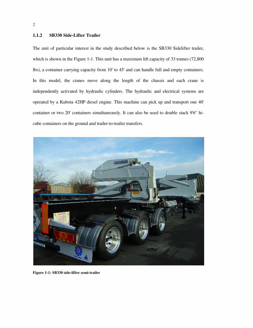
1.1.2 SB330 Side-Lifter Trailer

The unit of particular interest in the study described below is the SB330 Sidelifter trailer,

which is shown in the Figure 1-1. This unit has a maximum lift capacity of 33 tonnes (72,800

lbs), a container carrying capacity from 10' to 45' and can handle full and empty containers.

In this model, the cranes move along the length of the chassis and each crane is

independently activated by hydraulic cylinders. The hydraulic and electrical systems are

operated by a Kubota 42HP diesel engine. This machine can pick up and transport one 40'

container or two 20' containers simultaneously. It can also be used to double stack 9'6" hi-

cube containers on the ground and trailer-to-trailer transfers.

Figure 1-1: SB330 side-lifter semi-trailer

3

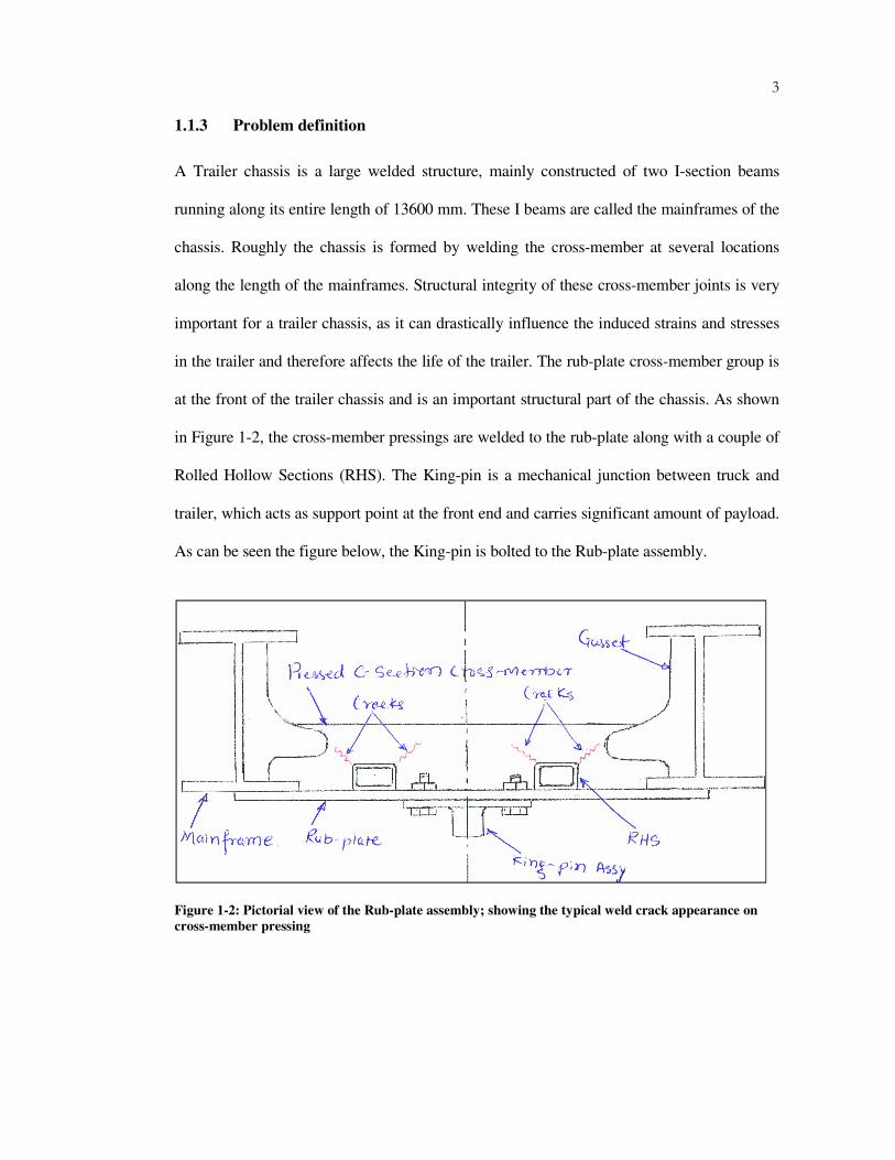
1.1.3 Problem definition

A Trailer chassis is a large welded structure, mainly constructed of two I-section beams

running along its entire length of 13600 mm. These I beams are called the mainframes of the

chassis. Roughly the chassis is formed by welding the cross-member at several locations

along the length of the mainframes. Structural integrity of these cross-member joints is very

important for a trailer chassis, as it can drastically influence the induced strains and stresses

in the trailer and therefore affects the life of the trailer. The rub-plate cross-member group is

at the front of the trailer chassis and is an important structural part of the chassis. As shown

in Figure 1-2, the cross-member pressings are welded to the rub-plate along with a couple of

Rolled Hollow Sections (RHS). The King-pin is a mechanical junction between truck and

trailer, which acts as support point at the front end and carries significant amount of payload.

As can be seen the figure below, the King-pin is bolted to the Rub-plate assembly.

Figure 1-2: Pictorial view of the Rub-plate assembly; showing the typical weld crack appearance on

cross-member pressing

4

In this particular SB330 trailer chassis, cracks have appeared in various cross-member joints

in early stages of its lifetime. Pictorial view of the cracks on the rub-plate cross-member

pressing is shown in Figure 1-2. Also, cracks ground for welding is shown in Figure 1-3. So

far a quick fix at service stations has eliminated all the cracks in the cross-member joints.

An additional strengthening plate added to the cross-member pressing can be seen in Figure

1-4, which has eliminated further cracking of the cross-member pressing. However an

alternative design level solution is sought for the rub-plate cross-member group based on its

structural importance in the trailer chassis.

Figure 1-3: Cracks at the corner of the cross-member and RHS ground for welding is shown on the

actual trailer.

5

Figure 1-4: Showing the additional strengthening plates welded to the Rub-plate cross member

1.1.4 Speculations of cause

There are two main factors considered to be seriously contributing to the above explained

problem. The factors are explained below:

Firstly, when the trailer is transporting loaded container, it tends to deflect (bow and hog) up

and down at the unsupported span of the chassis. This is perhaps due to change in inertia

forces, which causes the swinging action to act like a cyclic loading on the chassis. Also a

frequent loading/unloading operation can produce the same effect on the chassis. Altogether

this may exceed the fatigue limit of the material causing failure due to fatigue.

Secondly, Yard manoeuvres are as important as on road movements of a trailer, it can be

crucial if certain aspects are considered such as lateral deflection of the chassis. When the

trailer moves in a congested yard environment, manoeuvres such as turning around a sharp

corner or reversing in a confined space could produce a bowing effect on the chassis. If the

intensity of the lateral deflection due to yard manoeuvres is very high it could cause the

6

working stress to exceed yield stress of the material or repeated yard manoeuvres could

cause cyclic effects on the chassis leading to fatigue failure.

1.2 Research objectives

• Investigate and confirm the reasons behind the rub-plate cross-member cracks.

• Conduct the static and fatigue analysis on the current design using FEA techniques.

• Restructuring the cross-member joint design to overcome the particular cracking

problem.

• Develop suitable finite element procedure, which can be incorporated into the

STEELBRO’s conventional product development process.

7

1.3 Outline of the thesis

This section provides an outline of the organization and brief description of the remaining

sections of the thesis.

The body of this thesis consists of mainly seven chapters as shown in Figure 1-5. Initially the

problem is defined and sufficient literature survey is done to identify and gain knowledge

form the previous research in the related field. Then a suitable problem approach is adopted

to solve the problem. An experimental method, which employs the strain gauge technology,

is also used to validate the FEA predicted results. A chapter wise briefing is as follows:

Chapter 2 discusses some of the relevant literature such as journal papers, publications,

articles, theses on finite element method, stress analysis, trailer design, Sub-modelling

technique in FEA, fatigue analysis and so on.

Chapter 3 details the physical structure of the trailer. It shows complete solid modelling of

the trailer and presents associated technical details up to the discretization stage of the finite

element analysis.

Chapter 4 covers the static structural analysis of the trailer. The analysis is performed on the

trailer for two cases namely, static loading/unloading and perceived “worst case” condition.

This chapter also includes discussion on the causes of the failure based on the results

obtained from the finite element analysis of the trailer.

Chapter 5 validates the finite element model used for the static analysis using ANSYS shape

checking feature and strain values recorded for the rosette strain gauges. It also reports the

differences between the analytically calculated stress values and the linear strain gauge

results.

Chapter 6 use finite element analysis technique for the fatigue analysis of the current design

to determine the fatigue life. It also includes the redesign of the problem area to overcome

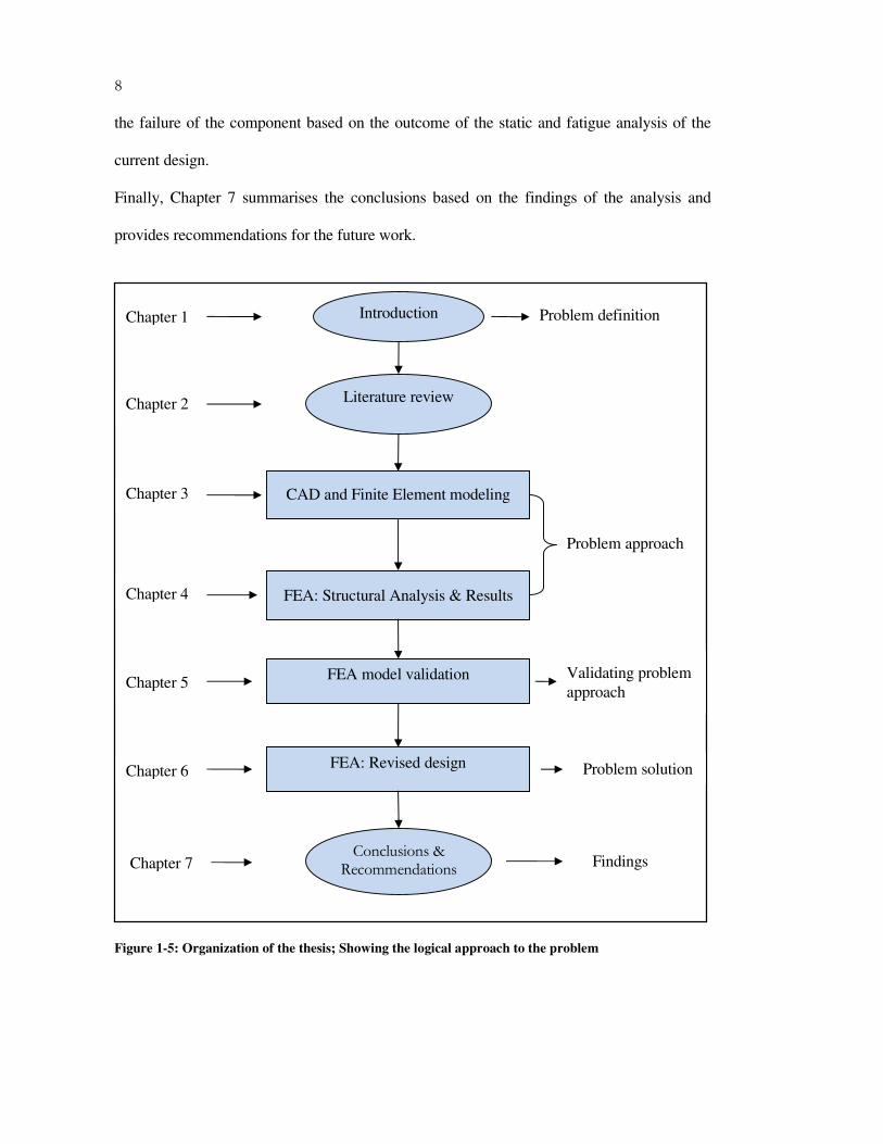
8

the failure of the component based on the outcome of the static and fatigue analysis of the

current design.

Finally, Chapter 7 summarises the conclusions based on the findings of the analysis and

provides recommendations for the future work.

Figure 1-5: Organization of the thesis; Showing the logical approach to the problem

Introduction

Literature review

CAD and Finite Element modeling

FEA: Structural Analysis & Results

FEA model validation

FEA: Revised design

Conclusions & Recommendations

Chapter 1

Chapter 2

Chapter 3

Chapter 4

Chapter 5

Chapter 6

Chapter 7

Problem definition

Problem approach

Problem solution

Findings

Validating problem

approach

9

1.4 Scope and limitations of the research

In this research the trailer design is verified for two important known loading conditions. The

outcome of the analysis could become the basis for further complex design analysis. In any

type of design analysis, engineering practice is to keep the working stress well below the

yield stress of the material. Therefore the approach followed in this study could be widely

used in trailer manufacturing industries.

In this study only linear elastic material model is used for the static analysis and non-linear

material behaviour is not considered, which could be important for further design analysis of

the structure. Also, the true characteristics of the shock absorbers in the suspension have not

been built into the model, which could be significant for further dynamic analysis of the

trailer. Finally, fatigue analysis performed on the current design is only based on FEA

method, which will have to be validated experimentally.

10

2 LITERATURE SURVEY

2.1 Introduction

The finite element method is now used in wide range of industries in research and product

development process. This is a result of continuous development of the technology over five

decades, ever since it was introduced in 1950s. In the past two decades, the technological

advancement in the field of the digital computers has turned finite element method into a

very sophisticated tool, which can analyze complex field problems. Hence rapid growth in

application of the FEA technology can be seen in this era. The advantages of using FEA

were soon realized in competitive industrial world and triggered research and development

within the industry for the effective use of the finite element tool. The investigation done in

this thesis is an ideal example of such a type. Scholarly and commercial research literatures

surveyed in the field of structural analysis using FEA indicates the commercial value of this

tool. Some of the researches, which are relevant to this research include static analysis, sub-

modeling, fatigue analysis, strain gauging, etc are briefed below.

Forest Engineering Research Institute of Canada (FERIC) has developed software for

designing light weight trailers for logging operations. This is interactive software based on

finite element analysis technique. To validate the trailer design software experiments were

conducted on the actual trailer for stress and deflection and also modal testing of the chassis

was carried out. For instance strain gauges and accelerometers were mounted on the chassis

to measure strain and acceleration at critical locations respectively. They found that the

experimental results obtained showed good correlation with the results of the trailer design

software and ANSYS, commercially available analysis software as well. Then prototype was

11

designed using trailer design software and manufactured. The experimental test showed the

results were well within the safe working limit [3].

According to Rahman, Tamin, and Kurdi (2008), highest stress point can be identified for

components by performing the stress analysis, which is essential for the fatigue life

prediction of components. In this research finite element analysis of the truck model is

performed using ABACUS analysis software. In the static structural analysis performed on

the truck, the static forces created by the truck body and the cargo are applied on the chassis.

Then the boundary condition resembling the physical situation is applied to constraint the

truck model. The model is discretized using 3D tetrahedral elements. The results showed the

highest stress point and maximum deflection in the chassis. The deflection is validated using

the analytical formula. As the highest stress point can be the initiation point for the fatigue

failure, this paper concludes with recommendation to reduce the magnitude of the stress at

the critical point [4].

According to Kassahun (2008), responses of the vehicle structural components to the static

and dynamic loads are very important to produce good quality vehicles with longer fatigue

life, greater strength, low weight and low cost. In this research this is achieved by studying

the structural response in terms of stress, strains, deflections and vibration and noise in the

components. In this study an ISUZU NPR commercial vehicle with van body is subjected to

the static and dynamic loading in finite element analysis software, ANSYS, and a van model

was also developed using the same software. Particularly static, modal and random vibration

analysis was done in ANSYS. As a result of these analyses the various structural components

of the van chassis, which are influenced by higher values of stress and deflection due to

different static and dynamic loading conditions, were identified [5].

12

Wang, and Rauch (2008) worked on fatigue analysis and design optimization of a trailer

hitch system. It involved testing the trailer hitch according to the customer specifications.

Locations of the failure were identified by the experimental testing. Design Modeler module

in ANSYS was used to model the global model of the trailer hitch. Then it was meshed using

uniform finite elements and a coarse finite element model was prepared. Later this model

was analyzed to identify the “hot spots”. It was found that the “hot spots” identified in the

analysis matched with the failure points identified in the experimental testing. The sub-

model was created form the global model of the trailer hitch at the area of interest and again

it was done in Design Modeler. The sub-model is then analyzed to obtain the local stress at

the area of interest. The data from the structural analysis then fed to the fatigue module of the

ANSYS to predict the fatigue life of the trailer hitch. Finally, parameter driven hitch

geometry was created and DesignXplorer ANSYS module was used to optimize the trailer

hitch design based on the simulation results [6].

Bekah, (2004), carried out fatigue analysis of a car door hinge using finite element analysis

and validated the results by experimental testing. This process involved modeling finite

element model of the door hinge. A couple of models were tried in the geometry check and

one of them was found more accurate. This led to the further verification in the static

analysis and one of the FE model was confirmed to be more accurate. The static analysis was

carried out on the FE model for uni-axial and multi-axial loading. The analysis was carried

out in MSC.NASRAN and the model was solved for stress and strains. The results obtained

from the static analysis were used in the fatigue analysis to predict the fatigue life of the door

hinge. Finally, on the basis of FE based fatigue analysis, the door hinge design was

optimized and fatigue life of the door hinge was improved [7].

13

Petracconi, Ferreira, and Palma (2009) presented a paper that investigated current life of a

rear tow hook assembly of a passenger car by experimental testing. It was found that the life

of the product was less than the expected life of the tow hook during service. Care was taken

to conduct the experimental testing according to the actual service condition. As result of the

testing failure region were identified. FE-based simulation of the tow hook confirmed the

failure region as it was identified in the experimental fatigue testing. Rosette strain gauges

were used to record the micro-strain at the failure region of the tow hook. The data was

recorded on a computer from the strain gauges through data acquisition system. Then the

fatigue life identified from the experimental fatigue testing is compared with the life

estimated from the FE-based simulation and it was found that the results are within the

acceptable limit. Based on this methodology new configurations of the tow hook were

simulation tested and best of design was proposed for manufacturing. Finally, the prototype

was experimentally tested for fatigue life and it was found that no cracks were found during

the expected service life of the tow hook [8].

Topac, Gunal, & Kuralay ( 2008) presented a paper that studied fatigue failure of a rear axle

housing and proposed a solution to increase its fatigue life. In this study prototype axle

housing was experimentally tested for fatigue life using hydraulic test rig. The results of the

test showed that the cracks appeared before the expected design life of the axle housing. The

next step in the research was to create the detailed model of the axle housing in the CATIA

V5R15 software. Then the solid model was imported into ANSYS Workbench 11 for the

static and fatigue analysis. The material properties and the S-N curve for the material were

obtained from the tensile test of the housing material test specimen. The FE-based fatigue

analysis performed in the ANSYS confirmed the critical region identified in the experimental

fatigue testing and the results showed that this is due to the stress concentration, which

14

reduced the expected life of the axle housing. Finally the study was concluded that the stress

concentration should be reduced to increase the fatigue life and proposed the design change

at the critical region and increase in the thickness of the reinforcement ring of the axle

housing [9].

Fermer & Svensson, ( 2001) presented a paper that discuses about FE-based fatigue analysis

methodology used in automotive industries. Generally spot welds and seam welds are

commonly used joining method in car and truck body building. The failures of these welds

have prompted continuous research and development in FE-based fatigue simulation to

minimize the cost of the production. This paper details few experiences of using FE-based

fatigue analysis in predicting fatigue life of the spot and seem welded joints. These analyses

showed that the method used for the fatigue analysis is good enough to be incorporated in the

design process. It also mentions about the growing trend of the finite element analysis in the

automotive industry. Finally, this paper conclude with the finding that the FE-based fatigue

life prediction of the weld in conjunction with the results obtained from the analytical

methods were in good correlation with the results obtained from the experimental fatigue

testing.[10]

Yongming, Startman, & Mahadevan, (2006) proposed a new multi-axial fatigue damage

model and “elasto-plastic” finite element model. In this paper a multi-axial fatigue damage

model was developed for railroad wheel, where complex rolling contact stresses are

involved, which is capable of predicting “both the initiation crack plane orientation and

fatigue initiation life”. In the next step of the research finite element model of the wheel/rail

contact was developed. This involved modeling a full scale model of the wheel/rail contact

and analyzing in ANSYS 7 software. In order to increase the efficiency and accuracy of the

finite element analysis, the sub-modeling technique is also included in the proposed finite

15

element model. Then the numerical example was used to qualitatively validate the proposed

models. Finally the proposed models were used to study the different parameters of the

wheel and its effects on the fatigue damage were investigated and recommendations were

suggested for the future work [11].

Ye & Moan, (2007) investigated aluminium box-stiffener /web frame connection for fatigue

life. Three types of designs used in this study these connections were designed in such a way

that the cost of fabrication could be reduced without compromising the fatigue strength.

Finite element analysis (FEA) and experimental fatigue tests were carried out to study the

static and fatigue behaviour of the connection. FEA analyzed the effect of weld parameters

and local geometry at the cracking area for stress gradient and stress concentration. Twelve

specimens of the three designs were experimentally tested for fatigue life. Experimental data

indicated that two of the three designs should be avoided due to possible defects introduced

by the welding procedure, which can reduce the fatigue life. Finally the study showed that

the size of the fillet weldment has a greater influence on the fatigue life of the joint [12].

Zhao, Li, & Shen, (2008) presented a paper on improving the fatigue life of the rubber mount

on the crack-shaft of an automobile wheel. In this research they investigated the fatigue crack

using the finite element model of the mount and the model was analyzed for fatigue in

MSC.MARC analysis software. Stress concentration was found at the interface of the rubber

and metal of the mount. Then the stress concentration was minimized by modifying the

structural parameters of the mount and the rubber material. As a result, fatigue life of the

rubber mount was increased. This new FEA process and methodology was also backed up by

experimental testing. Finally on this basis, a new FEA process and methodology was

proposed, which can improve product quality. The proposed technique was also cost

effective due to shortened product development cycle [13].

16

Karaoglu & Kuralay, (2002) conducted a study on stress analysis of a truck chassis with

riveted joints. The purpose of this study was to reduce the magnitude of the stress near the

riveted joints. Three geometric parameters of the components of the joints were varied and

analyzed in ANSYS version 5.3 analysis software. Three variables of the joints were

thickness of the sidebar and connection plate and length of the connection plate. During the

analysis it was found that increasing the sidebar thickness can reduce the stress but at the

consequence of high overall weight. This problem was overcome by just increasing the local

thickness of the sidebar using the local plate. Increasing the thickness of the connection plate

also reduced the stress in the connection plate with slightly increased stress in the sidebar. As

a final option, increase in the length of the connection plate also decreased the stress

distribution near the riveted joints. Finally, comparison of all three results of the analysis

concluded that stress near the riveted joints can be reduced by using local plate at the joints.

If not, increasing the length of the connection plate can be a better option to minimize the

stresses [14].

Colquhoun & Draper, (2000) presented a paper, which discusses the local strain-based

fatigue analysis using finite element model. In this analysis local strain based fatigue analysis

was integrated into software using finite element technique. This paper also discusses few

industrial experiences to validate the analysis. It was found that the experimental results were

in good agreement with the analysis results. The analysis process involved creating a CAD

model, exporting it to FEA software, initial stress analysis and then fatigue analysis. It was

found during the analysis that the fatigue results were mesh dependent and simple mesh can

estimate non-conservative fatigue life. This problem was overcome by using refined mesh.

Finally this paper concluded that the crack locations can be accurately determined and very

reliable fatigue life estimates can be done using finite element model [15].

17

Cowell, (2006) developed a methodology to predict the fatigue life of the rotary-wing

aircraft components using commercially available analysis software, namely, ANSYS and

Fe-safe. The primary objective of the research was to predict the fatigue life of the

components and confirm the suitability of the repaired ones for further use in the same

service conditions. Fatigue analysis of a flat plate with a centrally located hole is carried out

using this methodology and predicted fatigue life the plate is compared with the simulated

life obtained from stress and strain fatigue life algorithms based on previously published

experimental data. The predicted fatigue life found to be in good agreement with the

simulated results. When this methodology is applied to the helicopter main gear drag beam,

it was found to be effective in identifying the influence of beam thickness on fatigue life of

the component. Finally, it was concluded that developed methodology was effective enough

to predict the fatigue life of the aircraft components and also can be used to confirm the

continuous use of the repaired parts [16].

He, Wang, & Gao, (2010) investigated a failure of an automobile damper spring tower. In

this investigation, firstly, the service conditions of the suspension assembly were identified

in order to establish the failure analysis procedure. Then the finite element analysis was done

to determine the static stress distribution on the damper spring tower. Later the strain gauges

were mounted on the critical location to record the strain gauge signals during the service

conditions. The data available from the strain gauges and the strain-life approach was used to

predict the fatigue life of the component and compared with the failure records. The

estimated life calculated from the damper spring tower with broken damper spring test was

found to be in good agreement with the failure records. Thus the research showed that the

failure of the damper spring tower was due to the early failure of the spring damper and

finally, the study recommended further test to improve the spring damper [17].

18

Palma & Santos, (2002) conducted a fatigue damage analysis of an automobile stabilizer bar.

In this research fatigue damage was calculated using a “linear damage rule” with the data

obtained from experimental test performed in the laboratory and the actual service

environment. The results were also verified by analytical method. Finite element analysis

was used to identify the critical stress locations on the stabilizer bar to mount the strain

gauges. The comparison of the results of the stress analysis from all the methods used in this

study showed that the magnitude of the stress distribution was similar. Finally the fatigue

damage and life of the stabilizer bar was calculated for extreme field conditions and a fatigue

failure criterion was set for laboratory testing conditions [18].

19

3 FEA: CAD AND FINITE ELEMENT MODELING

3.1 Introduction

The Finite Element Analysis (FEA) or Finite Element Method (FEM) is a numerical

technique, which could give near accurate solutions to complex field problems. Basically this

method involves dividing the complex structures into known number of smaller structures or

elements. This ability of the method is called discretization or meshing, which makes the

technique more effective in analyzing irregular shaped structures in a variety verity of

engineering problems [19]. Mathematically it is nothing but representing most of physical

problems in terms of mathematical models formed by differential and integral equations.

Complexities such as irregular shape of the object or boundary conditions involved in the

physical problems can make these equations almost impossible to solve directly. In this

situation finite element analysis technique is adopted to obtain near accurate solution for the

physical problem by approximately solving the governing equations, which could not be

solved otherwise [20].

The traditional product development process is based on fundamental engineering equations

and effective in analyzing regular shaped simple problems. However for complex physical

problems the design process is more dependent on extensive testing, which normally makes

the process expensive. The modern product development process with FEA technology does

not eliminate the product testing process, but its ability to analyze complex physical problem

easily and effectively can reduce the initial prototype testing in the design stages of the

product development process [1]. This makes FEA technology valuable in today’s

competitive industrial environment. Therefore in this research the solution is sought for a

structural problem, originally designed by the traditional method. The following section

20

discusses how the FEA technology is adopted in the product development process of the

trailer, which is originally designed by the traditional product development process.

3.2 Overview of the FEA Process

The outline of the finite element analysis procedure used in this research is shown in Figure

3-1. The complete process could be categorized into two main objectives; Firstly, the design

analysis stage and secondly, the design revision stage. The design analysis stage can be seen

as two loops, first, an inner loop and second, an outer loop. The inner loop is responsible for

achieving desirable accuracy of the finite element model and outer loop is responsible for

achieving good quality model for the analysis. Therefore these two loops collectively

contribute to the accuracy of the final solution. [20] The verification step in the design

analysis decides which loop the analysis will get into. This decision is mainly based on

factors such as maximum stress, visual inspection of the discretized model and quality of the

element used for finite element modeling. In the first stage of the FEA process, it is

necessary to analyze the existing or initial design in order to determine the causes of the

problem, which could indicate the right direction to achieve better design against failure and

provide solution to the problem. This is because the revised design strategy solely depends

on the results of the initial assessment of the current design. The initial analysis of the trailer

involves understanding the physical problem, constructing the CAD model of the trailer,

finite element modeling of the CAD model, and, stress analysis of the trailer model using

ANSYS software. These topics are explained in their own sections and outcome of the stress

analysis dictated the design improvement, which is discussed later in chapter 6, in context

with the stress analysis results obtained for the trailer. But for now the first stages of the FEA

analysis is explained in detail in the following sections.

21

Figure 3-1: Overview of the FEA process [20] [21]

Yes

Option 2 No

Pre-processor Solver Postprocessor

Physical Problem

Revise FEA-Model

Design Improvisation:

Fatigue Analysis & Redesign

Terminate: Improved design

Construct/Change CAD Model

Improve model

Yes No

Computer software

Refine Analysis

No O

pti

on 1

Verification: Stress

convergence Mesh quality

Prepare FEA

Model

Display FE results:

Stress

Solve Mathematical/FEA Model

22

3.3 Building the Model in the CAD system for FEA

The seamless integration of FEA into the current product development process of the

company can only be achieved if CAD and FEA activities are co-linear. In a company like

STEELBRO, where design engineer and design analyst are a single role, there is a good

opportunity to build CAD geometry best suited for FEA modelling, which could be used in

the production line after the successful completion of the analysis. The ideal conditions for

using the CAD model for FEA and all downstream applications with minimum effort is

achieved if CAD modeling is done with either 3D solids or surfaces to form to complete

volumes. The volumes created in this way can be meshed with tetrahedral 3D elements or

brick elements discussed later in this chapter or should be capable of providing mid-surface

extraction to create finite element model using shell elements [1]. This concept of utilising

same model for CAD and FEA is further explored to determine its suitability for the

company’s general purpose finite element analysis requirement and for trailer analysis as

well.

3.3.1 Physical Model of the trailer

The SB330 trailer chassis is a completely welded large structure as shown in Figure 3-2. It is

made up of A709M Grade 345w structural steel. The mechanical properties of the steel are

given in the Table 3-1. I-section beams called mainframes are the main structural members

of the trailer. These mainframes are connected together at various locations using structural

members such as plates, rectangular hollow sections and C-sections. The suspension is

welded at the rear of the chassis.

23

Modulus of Elasticity (E) MPa

Poisson Ratio ( ν)- typical value for steel

Yield Stress (σy) MPa

186200 0.29 353

Table 3-1: showing the mechanical properties of A709M Grade 345 W [29]

3.3.2 Modeling the Geometry

The aim of this section is to create an understanding of the necessity of building the solid

model for FEA use. However, the same model should also be able to create production

drawings with no or little effort. This could be achieved if the solid model is built with the

consideration of the downstream applications, for example using proper parent-child

relationship in feature building, which could be used to suppress features not necessary in

FEA modelling. To satisfy finite element modelling needs of the solid model, a clean

geometry is essential. Clean geometries can be built by building the solid models with

features, which enhances the chances of quality FEA meshing without compromising the

accuracy of the solid model. This can be achieved by modelling the features in such a way

that the solid model does not challenge the meshing process, but allows the creation of

quality elements and manipulating the solid model in such a way that it does not affect the

structural integrity of the part, for instance by simplification of the part away from the area of

interest [1].

The objective of building CAD model for FEA is to ensure a good quality mesh is produced

in the finite element modelling of the solid model. The first step in this process is to identify

the features that could potentially lead to a poor mesh. One of the very common solid

modeling issues from the point of view of FEA use of the solid model is short edges and

sliver surfaces, which were frequently encountered in this project’s solid modelling. An

example of such a problem is shown in Figure 3-3.

24

Figure 3-2: 2D drawing of the SB330 trailer showing the 20' and 40' container loading positions.

25

Figure 3-3: showing the potential sliver geometry in the filet feature of the weld-beed in the solid

model.

Normally in CAD model filet edges close to the other edges of the geometry or misalignment

of the features can create short edges. If such edges are smaller than the smallest edge of the

model or nominal element size in a mesh, it could create element distortion, where one edge

of the element is much shorter than the others. Similarly Sliver surfaces are narrow faces

with very high aspect ratio. More often, automeshers create sliver surfaces by placing very

flat element on short edges encountered in the geometry during meshing. Therefore, as a

good modeling practice, the length of the edges in the solid model should be kept more than

one-third of the desired element edge length of the finite element mesh [1].

26

3.3.3 Finalising the trailer geometry for FEA

Physical model of the whole trailer including suspension was modelled using SolidWorks

modelling software. The assembly modelling was done such a way that the co-ordinate

system of the physical model coincides with the co-ordinate system of the FEA model later

in the simulation environment for the simplicity of the analysis. The suspension model was

obtained from Hendrickson Asia Pacific Pty Ltd. The imported suspension model was

converted from surface body to solid body with the intension of using it as a rigid body in the

analysis. The primary objective of this research is to study and analyze the chassis of the

trailer. The suspension being the third party component for STEELBRO, it is not of great

importance to the company. However, in reality, suspension does play an important role in

the load distribution along the length of the chassis. Therefore considering the geometric

importance of the suspension in relation with the chassis, the suspension is modeled as a

single component. Parent-child relations are suitably managed to create parts for the chassis

considering the future needs of the FEA modeling, where parts or features of the component

that could be insignificant for the finite element analysis can be easily suppressed. The

chassis is modeled as an assembly of various structural members. The entire SolidWorks

assembly is saved as a parasolid file, which can be imported into the Ansys Design Modeler

software. This is done due to an ANSYS license restriction to import SolidWorks files

directly into Design Modeler environment. Design Modeler was used to prepare the solid

model for the analysis due to its greater ability to simplify and prepare CAD model for

further analysis in the ANSYS simulation, e.g. “Inprint” faces, which allows applying point

load on a surface. “Inprint” faces are created on the chassis at the 20’ and 40’ container

mounting positions. Finalized geometry of the trailer which is used for the analysis is shown

in Figure 3-4.

27

Figure 3-4: Showing the Final geometry for the FEA

3.4 Modelling with Finite Elements

The accuracy of the solution of the physical problem depends on the finite element

modelling of the problem and accuracy of the finite element model depends on how well it

represents the physical behaviour of the problem, which is largely dependent on the quality

and quantity of the elements used to build the finite element model. If care is not taken, the

model can be too inaccurate or can waste valuable computer resources and time during the

analysis. As the whole modeling process is numerical approximation using polynomial

interpolation at elemental nodes [21][22], it is necessary to understand the capabilities and

limitation of the finite element method in order to ensure the proper finite element modelling

techniques are employed to achieve the desired results.

The following illustrative example obtained from the text book of ‘ANSYS Workbench

Software Tutorial’ [23] is used to demonstrate the effect of proper finite element modelling

technique in combination with proper element type on the accuracy of the results, which is

28

compared with the analytical solution calculated for the problem. It also serves as a basis for

the more complex analysis performed on the trailer chassis in the following chapter.

3.4.1 Analytical approach

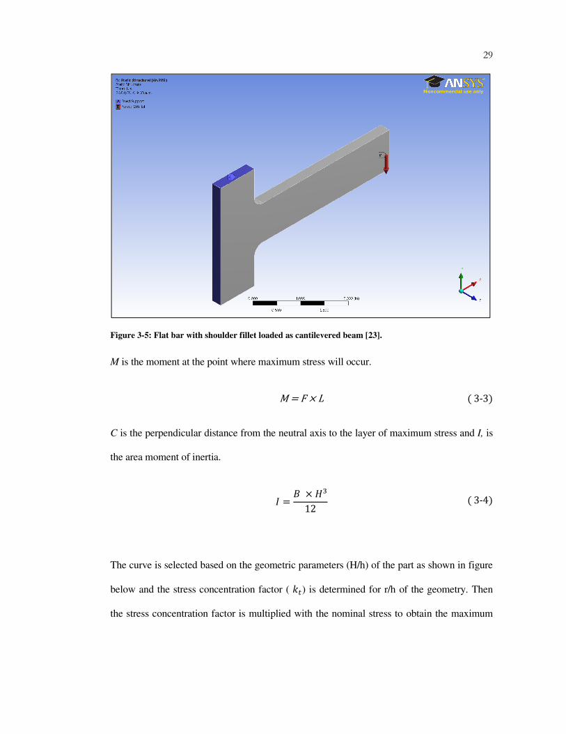
The physical object shown in the Figure 3-5 is a bar with shoulder fillet, loaded as a

cantilevered beam. Three faces at left side of the flat bar are fixed; Left, top and bottom face.

The free end of the part on the right face carries a bending load acting vertically downward

can be seen in Figure 3-5. The shape of the geometry shown in the figure can be assumed as

a cut off part from the rectangular plate. In this case, the total load carried by the original

rectangular plate cross section will now be loaded on to the remaining cross section of the

plate. Therefore the uniformly distributed stress over the original area of the plate now will

be concentrated at the change of cross section of the part. [24] Hence it can be predicted that

the stress concentration will occur at the fillet region of the part, where the fillet meets the

rectangular section of the unsupported part of the flat bar. The maximum stress at this

location can be calculated from elasticity theory using stress concentration factor (��) and the

equation (3.1). Stress concentration factor ( ��) can be obtained from the graph shown in

Figure 3-6 [23]. The graph is plotted based on theoretical elastic, homogeneous and isotropic

material considering only the shape of the part.

���� = �� × ��"� (3-1)

Where,

��"� = 5 × �6 (3-2)

29

Figure 3-5: Flat bar with shoulder fillet loaded as cantilevered beam [23].

M is the moment at the point where maximum stress will occur.

M=F×L (3-3)

C is the perpendicular distance from the neutral axis to the layer of maximum stress and I, is

the area moment of inertia.

6 = : × �&12 (3-4)

The curve is selected based on the geometric parameters (H/h) of the part as shown in figure

below and the stress concentration factor ( ��) is determined for r/h of the geometry. Then

the stress concentration factor is multiplied with the nominal stress to obtain the maximum

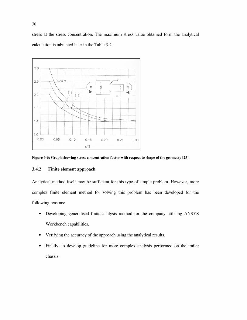
30

stress at the stress concentration. The maximum stress value obtained form the analytical

calculation is tabulated later in the Table 3-2.

Figure 3-6: Graph showing stress concentration factor with respect to shape of the geometry [23]

3.4.2 Finite element approach

Analytical method itself may be sufficient for this type of simple problem. However, more

complex finite element method for solving this problem has been developed for the

following reasons:

• Developing generalised finite analysis method for the company utilising ANSYS

Workbench capabilities.

• Verifying the accuracy of the approach using the analytical results.

• Finally, to develop guideline for more complex analysis performed on the trailer

chassis.

31

3.4.2.1 Automeshing solid model using ANSYS workbench

Meshing is the process of dividing the solids or surfaces into discrete elements. It can be

either done manually or automatically. In case of manual discretization, the model will be

built by specifying the coordinates of each nodes and connecting the nodes to form the

elements, which will eventually acquire the shape of the object being discretized. This

process can be tedious and laborious and may not be feasible for very complex parts. On the

other hand, ANSYS workbench automeshing algorithm extracts the geometric information

from the CAD model submitted for the analysis and uses the default setting based on the

analysis type to produces the mesh. [23] This mesh can be altered after the initial assessment

of the discretized model. The quality of the finite element model produced by automeshing is

governed by three factors. Namely, quality of the CAD model, mesh refinement at the

transition between the features, and the meshing algorithm’s ability to reform badly shaped

elements. Although the last one is not user controlled, the first two factors greatly influence

the third factor and in turn the accuracy of the result [1]. Building the proper geometry for

FEA use is already discussed in the previous section and the following sections deals with

the second factor. This includes element type and modelling procedure using ANSYS

meshing algorithm to obtain accurate solution.

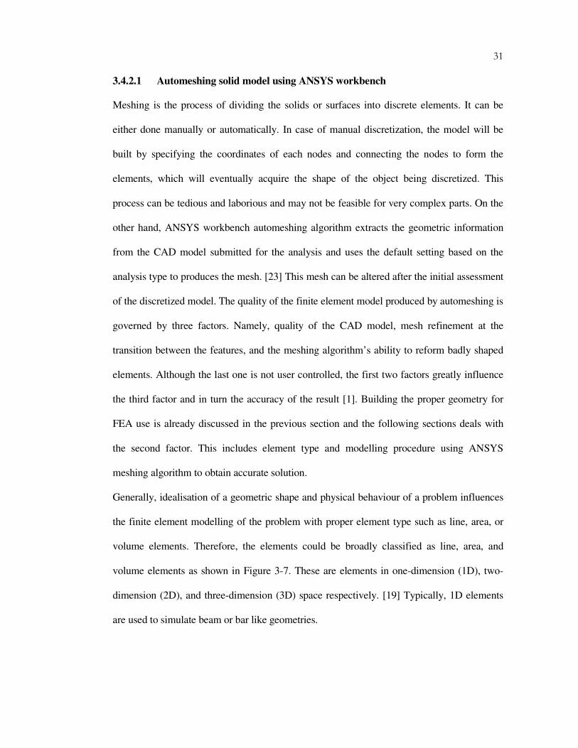
Generally, idealisation of a geometric shape and physical behaviour of a problem influences

the finite element modelling of the problem with proper element type such as line, area, or

volume elements. Therefore, the elements could be broadly classified as line, area, and

volume elements as shown in Figure 3-7. These are elements in one-dimension (1D), two-

dimension (2D), and three-dimension (3D) space respectively. [19] Typically, 1D elements

are used to simulate beam or bar like geometries.

32

Figure 3-7: showing the common type of elements used in FEA. [19]

The shell can be categorised as area element with a small thickness with respect to its area

and normally ideal for plate like geometries. For objects with symmetrical geometries, the

shell elements can be effectively utilised at a cost of mid-surface creation for the parts. This

process can be laborious and tedious for complex parts even with symmetry. This was

realised when an effort was made to create the surface geometry for the semi-trailer chassis.

The next obvious choice is 3D elements, which appear suitable for the company’s general

purposes and short product development cycle. Solid elements suit the company’s interest of

using the CAD model with little or no preparation for the analysis. Even though solid

elements are more resource intensive, it is possible to make the process less resource

intensive and achieve good quality results with special modelling technique like the sub-

modeling technique used in this project.

ANSYS Workbench pre-processor algorithm can default select solid elements depending on

the model to be analysed and provides options to select suitable elements. In order to analyse

33

the plate problem both default as well as user selection settings were used in the analysis.

Tetrahedron and hexahedron solid elements are considered for the analysis and the result of

the analysis is compared with the analytical solution obtained in the previous section. An

overview of different solid elements and its suitability for the analysis is discussed in the

following sections.

Constant strain Tetrahedron: The 4-node tetrahedron element is shown in Figure 3-8.

Each corner of the element has a node with three displacement degrees of freedom in X, Y,

and Z direction. In total, it has 12 displacement degrees of freedom for an element. The

element is a first order element and computes only a constant strain over span of the element.

Therefore, the element may be suitable where the strain is nearly constant for the length of

the element. The element is also inaccurate in modelling physical problem involving bending

and torsion, if the axis of such forces passing through or close to the element [21]. Therefore,

it may not be a good choice to use this element in the plate analysis as bending is involved.

Figure 3-8: 3D 4-node tetrahedron element

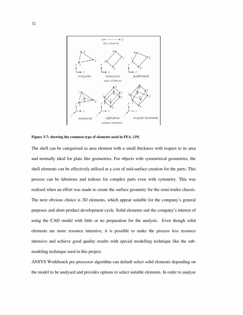
Linear strain tetrahedron: Linear strain 10-node tetrahedron is shown in Figure 3-9 below.

ANSYS identifies the element as SOLID187 and describes as 3D 10-node tetrahedral

structural solid element. The element has three displacement degrees of freedom at each

34 node in x, y, and z direction. In total,

element. It’s a higher order element with quadratic displacement behaviour, capable of

meshing irregular shapes modelled from CAD systems. The element is also capable of being

used in a situation of plasticity, creep, stress stiffening, large deflection

capabilities [26]. In addition, the ability to compute linear strain along the length of the

element enables it to model the bending situation more accuratel

element may be used for the analysis of the plate problem, where bending is involved.

Figure 3-9: 3D 10-node tetrahedron element

Trilinear Hexahedron: This element is popularly known as 8

in Figure 3-10. In ANSYS, the element is identified as SOLID185 and described as 3

node structural solid. The element has three translation degrees of freedom at each node in

X, Y, and Z direction. In total the element has 24

translation formulation of the element is

edges of the element remains straight during deformation

bending. Therefore, the element is unable to rep

remedy for shear locking may be possible but seems

total, it has 30 degrees of freedom for 10 nodes of an

higher order element with quadratic displacement behaviour, capable of

meshing irregular shapes modelled from CAD systems. The element is also capable of being

n a situation of plasticity, creep, stress stiffening, large deflection, and large strain

In addition, the ability to compute linear strain along the length of the

element enables it to model the bending situation more accurately [21]. Therefore this

for the analysis of the plate problem, where bending is involved.

element [26]

element is popularly known as 8-node brick element as shown

element is identified as SOLID185 and described as 3

The element has three translation degrees of freedom at each node in

otal the element has 24 translation degrees of freedom [26]

translation formulation of the element is missing few quadratic modes due to which, the

straight during deformation and undergoes shear locking in

the element is unable to represent beam behaviour very well [21]

locking may be possible but seems unnecessary when higher order

it has 30 degrees of freedom for 10 nodes of an

higher order element with quadratic displacement behaviour, capable of

meshing irregular shapes modelled from CAD systems. The element is also capable of being

, and large strain

In addition, the ability to compute linear strain along the length of the

herefore this

for the analysis of the plate problem, where bending is involved.

node brick element as shown

element is identified as SOLID185 and described as 3-D 8-

The element has three translation degrees of freedom at each node in

26]. The

due to which, the

undergoes shear locking in

[21]. The

when higher order

hexahedron element is available.

tetrahedron with 6-node wedge element, by collapsing two of its edges.

Figure 3-10: 3D 8-node hexahedron element

Quadratic Hexahedron: this element is shown in

and described as 3D 20-node structural solid in ANSYS workbench product. It is

order element with quadratic displacement be

node at every corner of the element and a mid

has three translation degrees of freedom at every node making up

freedom for the element. The mid

curved edges. When the element is rectangular, it is able to compute linear strain field more

correctly for the length of the element. Similar to linear strain tetrahedron, it is capable of

supporting plasticity, large defl

solid models produced form CAD packages. [26]

wedge element and 13-node pyramid element, when hex

analysis in ANSYS workbench.

hexahedron element is available. In ANSYS, it is possible to use the element as tri

node wedge element, by collapsing two of its edges.

node hexahedron element [26]

this element is shown in Figure 3-11. It is identified as SOLID186

node structural solid in ANSYS workbench product. It is

order element with quadratic displacement behaviour. As shown in the abov

node at every corner of the element and a mid-side node on the every edge of the element. It

has three translation degrees of freedom at every node making up total 48 degrees of

freedom for the element. The mid-side node of the element could be used to form straight or

curved edges. When the element is rectangular, it is able to compute linear strain field more

length of the element. Similar to linear strain tetrahedron, it is capable of

supporting plasticity, large deflection, large strain, etc and it is well suitable for modeling

solid models produced form CAD packages. [26] The element can be modified to 15

node pyramid element, when hex-dominant mesh is selected for the

bench.

35

In ANSYS, it is possible to use the element as tri-linear

. It is identified as SOLID186

node structural solid in ANSYS workbench product. It is a higher

haviour. As shown in the above figure, it has a

side node on the every edge of the element. It

total 48 degrees of

be used to form straight or

curved edges. When the element is rectangular, it is able to compute linear strain field more

length of the element. Similar to linear strain tetrahedron, it is capable of

ection, large strain, etc and it is well suitable for modeling

element can be modified to 15-node

dominant mesh is selected for the

36

Figure 3-11: 3D 20-node hexahedron solid element

From the above discussion of the solid elements available

that the use of higher order elements such as linear strain tetrahedron and quadratic

hexahedron may improve result quality

analysis. Figure 3-12 shows the 20-node hexahedron mesh produced by ANSYS Workbench

default setting and Figure 3-13 shows the 10

the user element setting to tetrahedron respectively.

node hexahedron solid element [26]

From the above discussion of the solid elements available in ANSYS workbench, it is seen

use of higher order elements such as linear strain tetrahedron and quadratic

improve result quality and therefore, these elements selected for further

node hexahedron mesh produced by ANSYS Workbench

shows the 10-node tetrahedron mesh produced by changing

the user element setting to tetrahedron respectively.

ANSYS workbench, it is seen

use of higher order elements such as linear strain tetrahedron and quadratic

selected for further

node hexahedron mesh produced by ANSYS Workbench

node tetrahedron mesh produced by changing

37

Figure 3-12: showing the plate meshed with 20-node hexahedron elements

Figure 3-13: showing the part meshed with 10-node tetrahedron elements

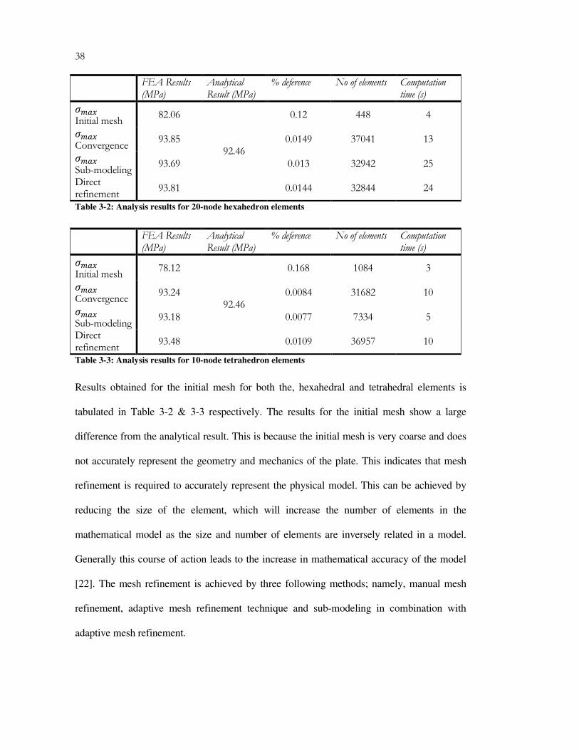
38

FEA Results (MPa)

Analytical Result (MPa)

% deference No of elements Computation time (s)

���� Initial mesh

82.06

92.46

0.12 448 4

���� Convergence

93.85 0.0149 37041 13

���� Sub-modeling

93.69 0.013 32942 25

Direct refinement

93.81 0.0144 32844 24

Table 3-2: Analysis results for 20-node hexahedron elements

FEA Results (MPa)

Analytical Result (MPa)

% deference No of elements Computation time (s)

���� Initial mesh

78.12

92.46

0.168 1084 3

���� Convergence

93.24 0.0084 31682 10

���� Sub-modeling

93.18 0.0077 7334 5

Direct refinement

93.48 0.0109 36957 10

Table 3-3: Analysis results for 10-node tetrahedron elements

Results obtained for the initial mesh for both the, hexahedral and tetrahedral elements is

tabulated in Table 3-2 & 3-3 respectively. The results for the initial mesh show a large

difference from the analytical result. This is because the initial mesh is very coarse and does

not accurately represent the geometry and mechanics of the plate. This indicates that mesh

refinement is required to accurately represent the physical model. This can be achieved by

reducing the size of the element, which will increase the number of elements in the

mathematical model as the size and number of elements are inversely related in a model.

Generally this course of action leads to the increase in mathematical accuracy of the model

[22]. The mesh refinement is achieved by three following methods; namely, manual mesh

refinement, adaptive mesh refinement technique and sub-modeling in combination with

adaptive mesh refinement.

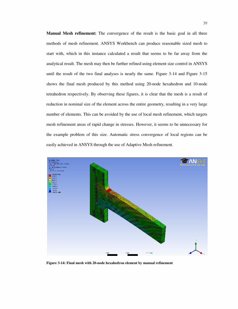
39

Manual Mesh refinement: The convergence of the result is the basic goal in all three

methods of mesh refinement. ANSYS Workbench can produce reasonable sized mesh to

start with, which in this instance calculated a result that seems to be far away from the

analytical result. The mesh may then be further refined using element size control in ANSYS

until the result of the two final analyses is nearly the same. Figure 3-14 and Figure 3-15

shows the final mesh produced by this method using 20-node hexahedron and 10-node

tetrahedron respectively. By observing these figures, it is clear that the mesh is a result of

reduction in nominal size of the element across the entire geometry, resulting in a very large

number of elements. This can be avoided by the use of local mesh refinement, which targets

mesh refinement areas of rapid change in stresses. However, it seems to be unnecessary for

the example problem of this size. Automatic stress convergence of local regions can be

easily achieved in ANSYS through the use of Adaptive Mesh refinement.

Figure 3-14: Final mesh with 20-node hexahedron element by manual refinement

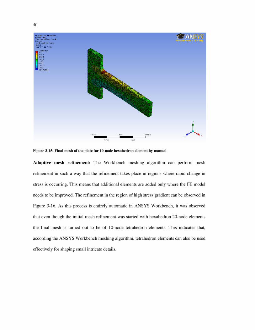
40

Figure 3-15: Final mesh of the plate for 10-node hexahedron element by manual

Adaptive mesh refinement: The Workbench meshing algorithm can perform mesh

refinement in such a way that the refinement takes place in regions where rapid change in

stress is occurring. This means that additional elements are added only where the FE model

needs to be improved. The refinement in the region of high stress gradient can be observed in

Figure 3-16. As this process is entirely automatic in ANSYS Workbench, it was observed

that even though the initial mesh refinement was started with hexahedron 20-node elements

the final mesh is turned out to be of 10-node tetrahedron elements. This indicates that,

according the ANSYS Workbench meshing algorithm, tetrahedron elements can also be used

effectively for shaping small intricate details.

41

Sub-modeling: Sub-modeling is based on St. Venant’s principal, which states that:

“If an actual distribution of forces is replaced by a statically equivalent system,

the distribution of stress and strain is altered only near the region of load

application”. [27]

According to this statement, stress concentration is a localised effect, which indicates that

accurate solution could be calculated for the area of interest, if the cut boundaries of the area

of interest covering the local stress are far away from the stress concentration. [27]

At this stage of the plate analysis, it is clear that the mesh density is extremely important;

Very coarse mesh can contain serious errors and finer mesh can require intensive computer

resources which make solution time relatively long. If the initial mesh reveals patches of

high stress gradient or any particular region of interest in a large structure, the sub-modelling

technique may be used to analyse the area of interest with very fine mesh. This technique

Figure 3-16: showing the fine mesh refinement only at the high stress gradient

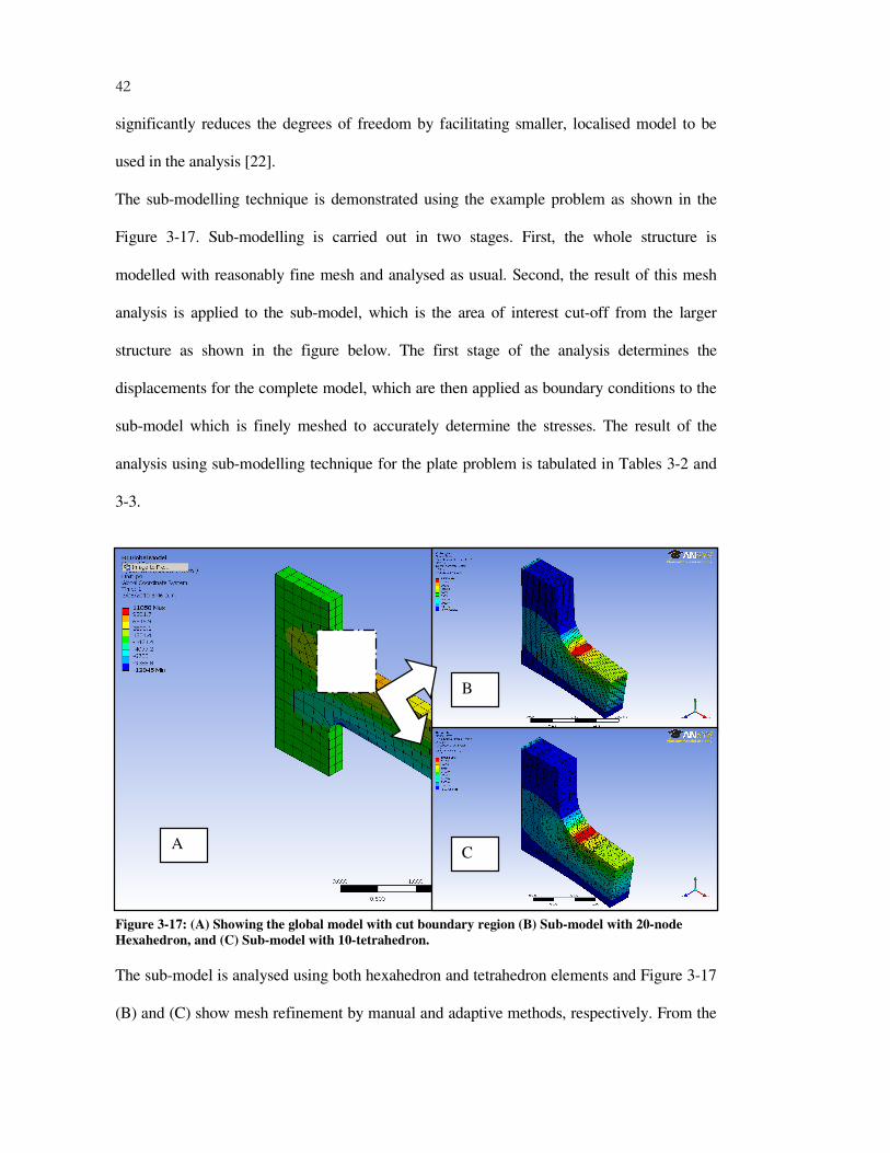
42

significantly reduces the degrees of freedom by facilitating smaller, localised model to be

used in the analysis [22].

The sub-modelling technique is demonstrated using the example problem as shown in the

Figure 3-17. Sub-modelling is carried out in two stages. First, the whole structure is

modelled with reasonably fine mesh and analysed as usual. Second, the result of this mesh

analysis is applied to the sub-model, which is the area of interest cut-off from the larger

structure as shown in the figure below. The first stage of the analysis determines the

displacements for the complete model, which are then applied as boundary conditions to the

sub-model which is finely meshed to accurately determine the stresses. The result of the

analysis using sub-modelling technique for the plate problem is tabulated in Tables 3-2 and

3-3.

The sub-model is analysed using both hexahedron and tetrahedron elements and Figure 3-17

(B) and (C) show mesh refinement by manual and adaptive methods, respectively. From the

A

B

C

Figure 3-17: (A) Showing the global model with cut boundary region (B) Sub-model with 20-node

Hexahedron, and (C) Sub-model with 10-tetrahedron.

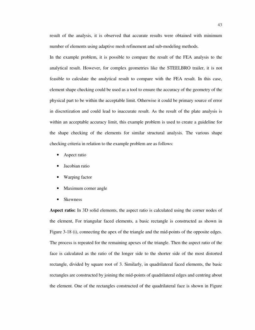
43

result of the analysis, it is observed that accurate results were obtained with minimum

number of elements using adaptive mesh refinement and sub-modeling methods.

In the example problem, it is possible to compare the result of the FEA analysis to the

analytical result. However, for complex geometries like the STEELBRO trailer, it is not

feasible to calculate the analytical result to compare with the FEA result. In this case,

element shape checking could be used as a tool to ensure the accuracy of the geometry of the

physical part to be within the acceptable limit. Otherwise it could be primary source of error

in discretization and could lead to inaccurate result. As the result of the plate analysis is

within an acceptable accuracy limit, this example problem is used to create a guideline for

the shape checking of the elements for similar structural analysis. The various shape

checking criteria in relation to the example problem are as follows:

• Aspect ratio

• Jacobian ratio

• Warping factor

• Maximum corner angle

• Skewness

Aspect ratio: In 3D solid elements, the aspect ratio is calculated using the corner nodes of

the element, For triangular faced elements, a basic rectangle is constructed as shown in

Figure 3-18 (i), connecting the apex of the triangle and the mid-points of the opposite edges.

The process is repeated for the remaining apexes of the triangle. Then the aspect ratio of the

face is calculated as the ratio of the longer side to the shorter side of the most distorted

rectangle, divided by square root of 3. Similarly, in quadrilateral faced elements, the basic

rectangles are constructed by joining the mid-points of quadrilateral edges and centring about

the element. One of the rectangles constructed of the quadrilateral face is shown in Figure

44

3-18 (ii). Then the aspect ratio for the face is calculated by dividing the longest edge to the

shortest edge of the most distorted rectangle. Likewise, the process is repeated for all the

faces of the quadrilateral element and the most distorted value of the aspect ratio among all

the faces of the element is considered the aspect ratio of the element. [26]

Figure 3-18: Aspect ratio calculation for (i) Triangle and (ii) Quadrilateral [26]

The ideal aspect ratio is 1 for a quadrilateral element and 1.15 for an equilateral triangle [22].

Large deviations from this will introduce some error into the calculations. The graph of

aspect ratios obtained for the example problem is shown in Figure 3-19 and Figure 3-20 for

hexahedral and tetrahedral elements respectively. In the graph of the hexahedral element, it is

observed that the aspect ratio for the hexahedral mesh ranged from 1 to 3. However, 90% of

the mesh has an aspect ratio close to 1. Similarly, the graph plotted for the tetrahedral mesh

of the same plate, shown in Figure 3-20, revealed that the aspect ratio ranged from 1 to 8.24,

with nearly 96% of the tetrahedral mesh is having an aspect ratio less than 3.

The percentage difference between the FEA result and the analytical result of the plate

problem and above observations confirms that aspect ratio from 1 to 3 can produce good

results and aspect ratios greater than 3 may be acceptable as long as it occurs away from the

area of interest [22].

O

R

P

Q

Midpoint

Rectangle

Triangle

Midpoint

Midpoint

Rectangle passing through midpoints

Quadrilateral

P

S

R

Q

O

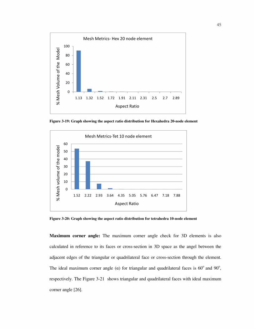
45

Figure 3-19: Graph showing the aspect ratio distribution for Hexahedra 20-node element

Figure 3-20: Graph showing the aspect ratio distribution for tetrahedra 10-node element

Maximum corner angle: The maximum corner angle check for 3D elements is also

calculated in reference to its faces or cross-section in 3D space as the angel between the

adjacent edges of the triangular or quadrilateral face or cross-section through the element.

The ideal maximum corner angle (α) for triangular and quadrilateral faces is 60o

and 90o,

respectively. The Figure 3-21 shows triangular and quadrilateral faces with ideal maximum

corner angle [26].

0

20

40

60

80

100

1.13 1.32 1.52 1.72 1.91 2.11 2.31 2.5 2.7 2.89

% M

esh

Vo

lum

e o

f th

e M

od

el

Aspect Ratio

Mesh Metrics- Hex 20 node element

0

10

20

30

40

50

60

1.52 2.22 2.93 3.64 4.35 5.05 5.76 6.47 7.18 7.88

% M

esh

vo

lum

e o

f th

e m

od

el

Aspect Ratio

Mesh Metrics-Tet 10 node element

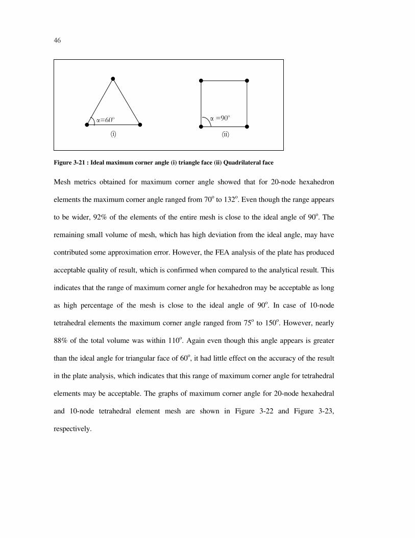
46

Figure 3-21 : Ideal maximum corner angle (i) triangle face (ii) Quadrilateral face

Mesh metrics obtained for maximum corner angle showed that for 20-node hexahedron

elements the maximum corner angle ranged from 70o to 132

o. Even though the range appears

to be wider, 92% of the elements of the entire mesh is close to the ideal angle of 90o. The

remaining small volume of mesh, which has high deviation from the ideal angle, may have

contributed some approximation error. However, the FEA analysis of the plate has produced

acceptable quality of result, which is confirmed when compared to the analytical result. This

indicates that the range of maximum corner angle for hexahedron may be acceptable as long

as high percentage of the mesh is close to the ideal angle of 90o. In case of 10-node

tetrahedral elements the maximum corner angle ranged from 75o to 150

o. However, nearly

88% of the total volume was within 110o. Again even though this angle appears is greater

than the ideal angle for triangular face of 60o, it had little effect on the accuracy of the result

in the plate analysis, which indicates that this range of maximum corner angle for tetrahedral

elements may be acceptable. The graphs of maximum corner angle for 20-node hexahedral

and 10-node tetrahedral element mesh are shown in Figure 3-22 and Figure 3-23,

respectively.

α =90o α=60o

(i) (ii)

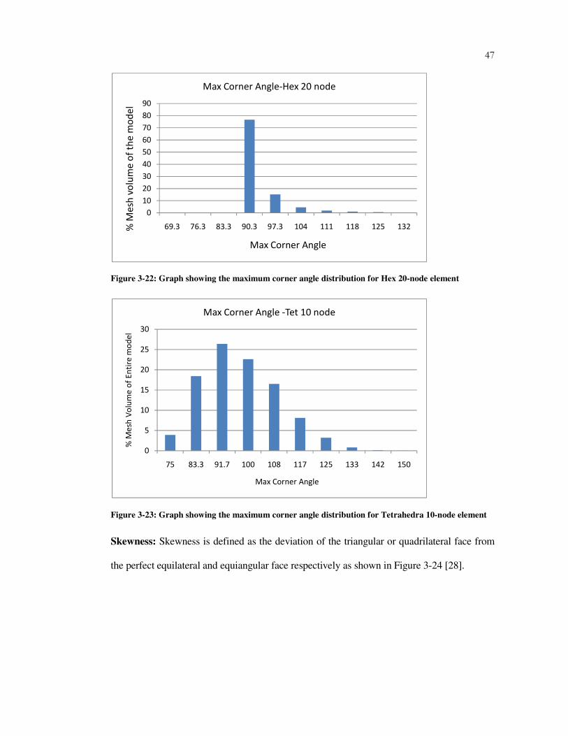
47

Figure 3-22: Graph showing the maximum corner angle distribution for Hex 20-node element

Figure 3-23: Graph showing the maximum corner angle distribution for Tetrahedra 10-node element

Skewness: Skewness is defined as the deviation of the triangular or quadrilateral face from

the perfect equilateral and equiangular face respectively as shown in Figure 3-24 [28].

0

10

20

30

40

50

60

70

80

90

69.3 76.3 83.3 90.3 97.3 104 111 118 125 132% M

esh

vo

lum

e o

f th

e m

od

el

Max Corner Angle

Max Corner Angle-Hex 20 node

0

5

10

15

20

25

30

75 83.3 91.7 100 108 117 125 133 142 150

% M

esh

Vo

lum

e o

f E

nti

re m

od

el

Max Corner Angle

Max Corner Angle -Tet 10 node

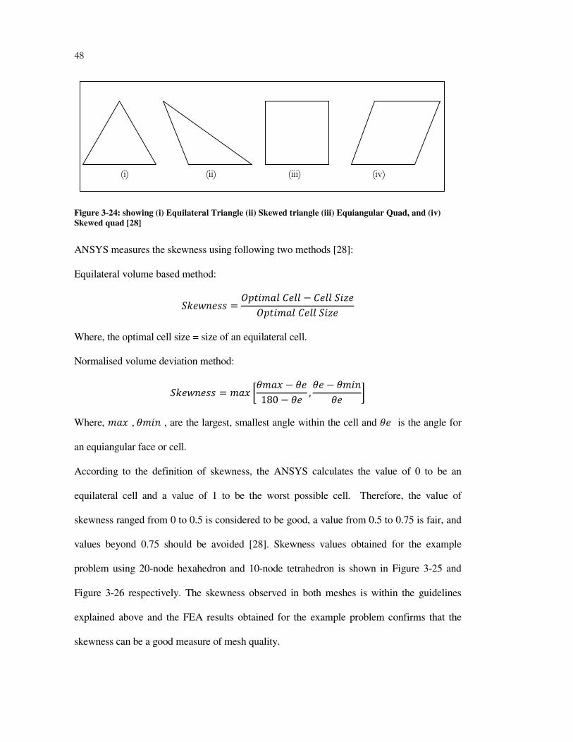
48

Figure 3-24: showing (i) Equilateral Triangle (ii) Skewed triangle (iii) Equiangular Quad, and (iv)

Skewed quad [28]

ANSYS measures the skewness using following two methods [28]:

Equilateral volume based method:

��<=�<�� = >�?@ABC<BB − C<BB�?E<>�?@ABC<BB�?E<

Where, the optimal cell size = size of an equilateral cell.

Normalised volume deviation method:

��<=�<�� = @A� FG@A� − G<180 − G< , G< − G@?�

G< J Where, @A� ,G@?� , are the largest, smallest angle within the cell and G< is the angle for

an equiangular face or cell.

According to the definition of skewness, the ANSYS calculates the value of 0 to be an

equilateral cell and a value of 1 to be the worst possible cell. Therefore, the value of

skewness ranged from 0 to 0.5 is considered to be good, a value from 0.5 to 0.75 is fair, and

values beyond 0.75 should be avoided [28]. Skewness values obtained for the example

problem using 20-node hexahedron and 10-node tetrahedron is shown in Figure 3-25 and

Figure 3-26 respectively. The skewness observed in both meshes is within the guidelines

explained above and the FEA results obtained for the example problem confirms that the

skewness can be a good measure of mesh quality.

(iv) (iii) (ii) (i)

49

Figure 3-25: Graph showing the skewness distribution for Hexahedra 20-node element

Figure 3-26: Graph showing the skewness distribution for Tetrahedra 10-node element

Warping factor: warping factor is only calculated for quadrilateral faces of the element. For

3D solid elements, as 4 nodes make up a face, the warping factor is calculated by dividing

the edge height difference of the twisted or lifted face by its square root of area. The warping

factor of 0 is a perfect shape of the element and a value beyond 1 is a poor shape. Figure

0

10

20

30

40

50

60

70

80

90

0.03 0.09 0.15 0.21 0.27 0.33 0.39 0.44 0.50 0.56% M

esh

Vo

lum

e o

f th

e M

od

el

Skewness

Skewness- Hex 20-node element

0

5

10

15

20

25

0.05 0.14 0.23 0.32 0.41 0.50 0.59 0.68 0.77 0.87% M

esh

Vo

lum

e o

f th

e M

od

el

Skesness

Skewness-Tet 10-node element

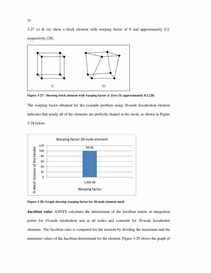
50

3-27 (i) & (ii) show a brick element with warping factor of 0 and approximately 0.2,

respectively [28].

Figure 3-27: Showing brick element with warping factor (i) Zero (ii) approximately 0.2 [28]

The warping factor obtained for the example problem using 20-node hexahedron element

indicates that nearly all of the elements are perfectly shaped in the mesh, as shown in Figure

3-28 below.

Figure 3-28: Graph showing warping factor for 20-node element mesh

Jacobian ratio: ANSYS calculates the determinant of the Jacobian matrix at integration

points for 10-node tetrahedron and at all nodes and centroids for 20-node hexahedral

elements. The Jacobian ratio is computed for the element by dividing the maximum and the

minimum values of the Jacobian determinant for the element. Figure 3-29 shows the graph of

99.96

0

20

40

60

80

100

120

5.00E-08

% M

esh

Vo

lum

e o

f th

e M

od

el

Warping factor

Warping factor-20 node element

(i) (ii)

51

the Jacobian ratio obtained for the 10-node tetrahedron and 20-node hexahedron. Form the

observation of the graphs; it is clear that the Jacobian ratio for both element types is close to

unity, which is an indication of well-shaped elements [28].

Figure 3-29: Graph showing the Jacobian ratio for the example problem for the element mesh

3.4.3 Discretization of the trailer solid model

The trailer solid model prepared according to the guidelines discussed in the CAD modeling

section is discretized using the knowledge gained by the analysis of the example problem in

the previous section. An initial mesh as shown in Figure 3-30 revealed that the model is very

large and requires too many elements if direct automeshing is applied. To avoid this over

discrimination, local meshing needed to be applied depending on the area of interest. The

area of interest in this study is the crack region at the rub-plate cross member as explained in

the Chapter 1. This area of interest is further discritised during the static analysis of the

trailer and will be discussed in the following chapter. The meshed finite element model of

the whole trailer chassis, which will be the “global model” in the finite element analysis, is

shown in Figure 3-30.

99.8

0

10

20

30

40

50

60

70

80

90

100

1.01

% M

esh

Vo

lum

e o

f th

e m

od

el

Jacobian Ratio

Jacobian Ratio- 10 node

Tetrahedron95.3

0

10

20

30

40

50

60

70

80

90

100

1.15%

Me

sh V

olu

me

of

the

mo

de

l

Jacobian Ratio

Jacobian Ratio- 20 node

Hexahedron

52

Figure 3-30: Initial mesh of the trailer solid model

53

4 FEA: STATIC STRUCTURAL ANALYSIS & RESULTS

4.1 Introduction

Generally, when designing mechanical structures, various analyses must be performed to

determine the strength of the structure against possible loads acting on the system. Among

these analyses, static analysis is the most common analysis performed on structures to

determine it’s strength against static loads acting on structure. This analysis is performed to

ensure the response of the structure to the static loads are within acceptable limit, otherwise

the structures would have little chance against other complex loads such as dynamic and/or

cyclic loads. Therefore, static analysis could be considered as the first step in structural

design analysis.

In this chapter, structural analysis is conducted on the trailer for two sets of static loading

situations. This is carried out to determine the effect of the static loading at the location of

the crack, as explained in the problem definition in the first chapter. The static structural

analysis is carried out with FEA numerical techniques using ANSYS finite element analysis

software. The systematic methodology for conducting the structural analysis of the trailer

using ANSYS software is proposed in this chapter. The procedure adopted in the analysis is

explained in the following sections.

54

4.2 Modes of operation of the trailer

The trailer model SB330 is designed for on-road container transport in New Zealand. It is

understood that the main use of the trailer is for transporting containers between shipyards

and warehouses in cities. The trailer typically carries 20' or 40' containers loaded within the

permissible payload. The trailer is equipped with two set of cranes, which facilitates loading

and unloading of containers. A typical trailer service would include loading the container at

the shipyard, carrying it to point of delivery and unloading with the help of cranes mounted

on the chassis or the reverse. Based on it’s normal service conditions, the following loading

conditions are considered for the analysis.

4.2.1 Normal loading/unloading condition

In this operating condition, the trailer is loaded with a 20'or 40' container. The containers are

positioned at “optimum” loading positions on the chassis as shown in Figure 3-2. The

container is placed on four docking points on the chassis and locked in its position by

devices called twist-locks. It is assumed that the load from the container is transferred to the

chassis at these four loading points. For this analysis, the maximum design load is applied on

the chassis and equally divided among the four docking points of the container. As

mentioned above, the cranes are also mounted on the chassis and the weight of the crane is

also equally divided between four contact points where it rests on the mainframe of the

chassis. The total load acting on the chassis is the weight of the container itself (in this case

maximum design load) and the weight of the two cranes. These loads acting on the chassis

form the force boundary condition on the chassis, as shown in Figures 4-1 & 4-2. The king-

pin connection to the trailer allows free rotation around Y-axis and Z-axis as shown in Figure

4-1 & Figure 4-2. The displacement and the rotation along the rest of the axes are fixed. This

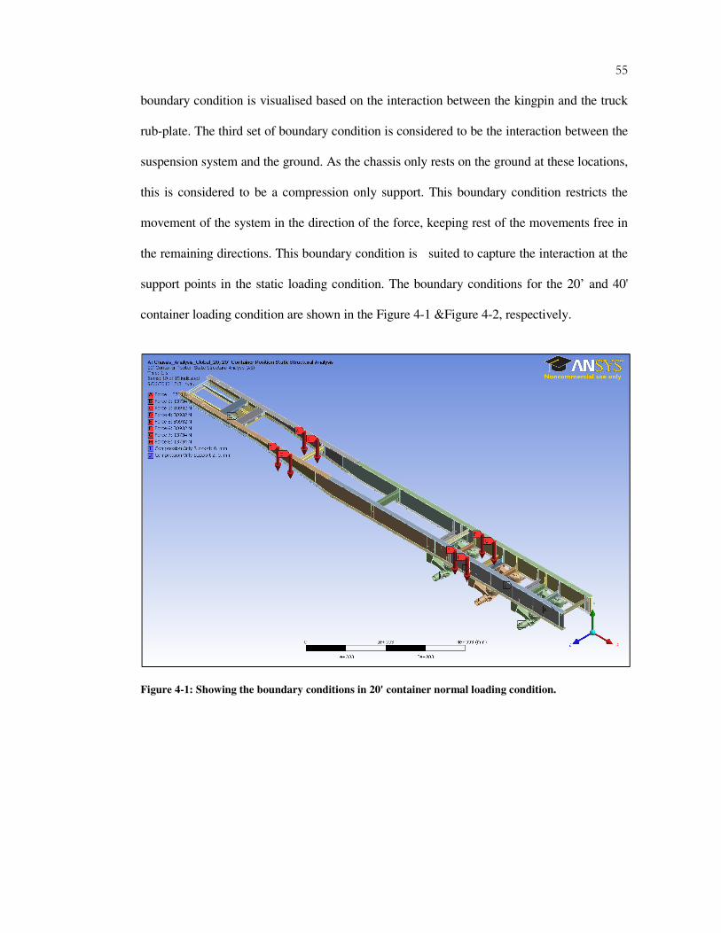
55

boundary condition is visualised based on the interaction between the kingpin and the truck

rub-plate. The third set of boundary condition is considered to be the interaction between the

suspension system and the ground. As the chassis only rests on the ground at these locations,

this is considered to be a compression only support. This boundary condition restricts the

movement of the system in the direction of the force, keeping rest of the movements free in

the remaining directions. This boundary condition is suited to capture the interaction at the

support points in the static loading condition. The boundary conditions for the 20’ and 40'

container loading condition are shown in the Figure 4-1 &Figure 4-2, respectively.

Figure 4-1: Showing the boundary conditions in 20' container normal loading condition.

56

Figure 4-2 Showing the boundary conditions in 40' container normal loading condition.

4.2.2 “Worst case” service condition

One possible reason for the appearance of the cracks at the rub-plate cross-member region is

the critical yard manoeuvres performed during service. In order to simulate the critical yard

manoeuvres, a hypothetical “worst case” scenario was developed where the trailer is

reversed into a shipyard gateway through the tightest possible corner. This condition is

simulated for both 20' and 40' container positions. This process is idealised as a quasi-static

case, where the trailer is being reversed at a very low speed. Meaning there is little or no

effect from dynamic forces. The pictorial representation of this situation is shown in Figure

4-3. As shown the trailer pivots at the king-pin. The pushing or pulling force at the king-pin

would produce turning moments at the wheels of the trailer, which could cause high stresses

at the rub-plate region. This boundary condition is simulated by applying the calculated

turning moment at the wheels and fixing the kingpin, as this would create a same effect of

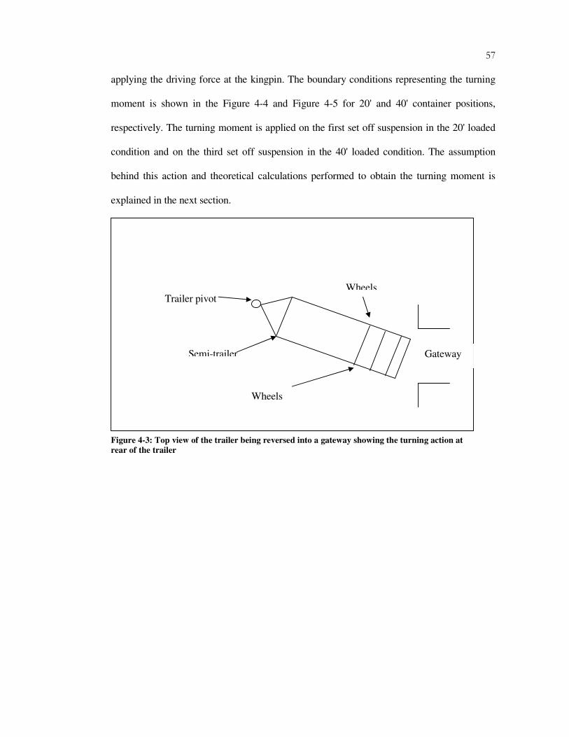
57

applying the driving force at the kingpin. The boundary conditions representing the turning

moment is shown in the Figure 4-4 and Figure 4-5 for 20' and 40' container positions,

respectively. The turning moment is applied on the first set off suspension in the 20' loaded

condition and on the third set off suspension in the 40' loaded condition. The assumption

behind this action and theoretical calculations performed to obtain the turning moment is

explained in the next section.

Trailer pivot

Semi-trailer

Wheels

Wheels

Gateway

Figure 4-3: Top view of the trailer being reversed into a gateway showing the turning action at

rear of the trailer

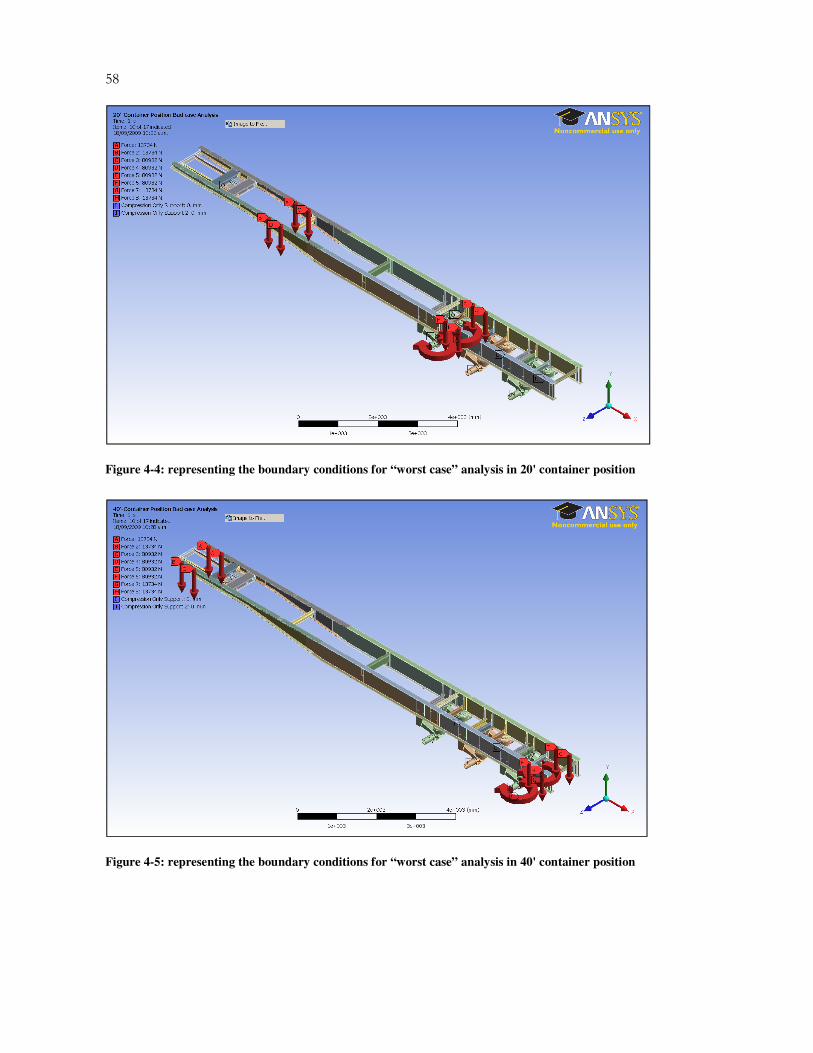
58

Figure 4-4: representing the boundary conditions for “worst case” analysis in 20' container position

Figure 4-5: representing the boundary conditions for “worst case” analysis in 40' container position

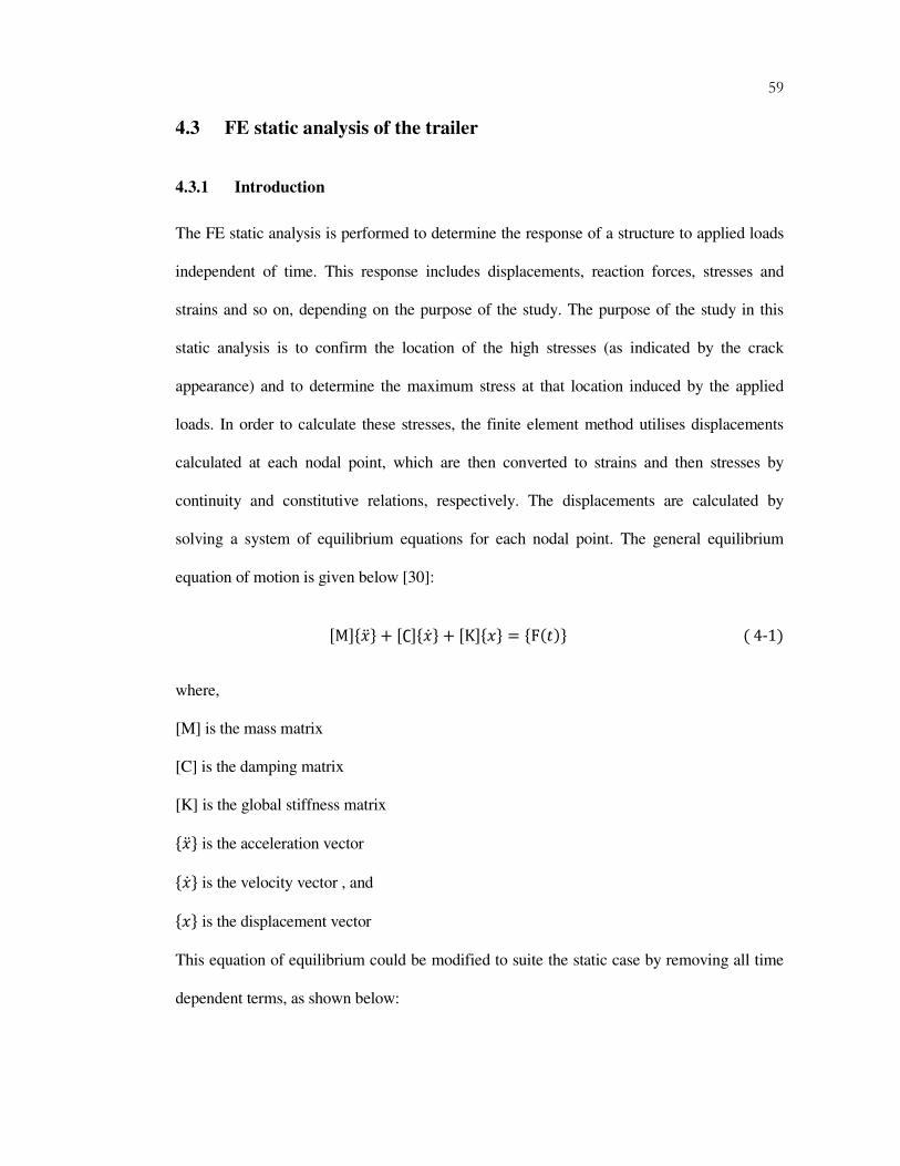
59

4.3 FE static analysis of the trailer

4.3.1 Introduction

The FE static analysis is performed to determine the response of a structure to applied loads

independent of time. This response includes displacements, reaction forces, stresses and

strains and so on, depending on the purpose of the study. The purpose of the study in this

static analysis is to confirm the location of the high stresses (as indicated by the crack

appearance) and to determine the maximum stress at that location induced by the applied

loads. In order to calculate these stresses, the finite element method utilises displacements

calculated at each nodal point, which are then converted to strains and then stresses by

continuity and constitutive relations, respectively. The displacements are calculated by

solving a system of equilibrium equations for each nodal point. The general equilibrium

equation of motion is given below [30]:

KML��� � + K∁L��� � + KKL��� = �F(�)� (4-1)

where,

[M] is the mass matrix

[C] is the damping matrix

[K] is the global stiffness matrix

��� � is the acceleration vector

��� � is the velocity vector , and

��� is the displacement vector

This equation of equilibrium could be modified to suite the static case by removing all time

dependent terms, as shown below:

60

KKL��� = �F� (4-2)

Where, the global stiffness matrix [K] is composed of elemental stiffness matrices[k]'. With

the application of known boundary conditions, the system of equation 4.2 is solved for

displacements at the nodes. These displacements are used to calculate strains and then

corresponding stresses are obtained. This numerical technique is performed on the trailer

using ANSYS workbench simulation environment to determine the stress distribution in the

structure.

4.3.2 Analysis strategy for the trailer

Success of the finite element method in today’s commercial world is largely because of the

computing power of the modern day computers. As the number of finite elements is directly

proportional to the accuracy of the mathematical model of the simulation environment,

computer memory and processing speed plays an important role in the analysis. It is

important to develop a finite element model that respects computing resources available for

the analysis. Without it, the analysis may not be feasible or it may be inaccurate. For

instance, the trailer is a large welded structure and analysing the full structure to obtain

accurate stresses across the entire structure may not be possible without exceeding the

elements or memory size limits. In this situation, the sub-modeling technique [31] offered in

ANSYS workbench appears to be a practical way reducing the size of the analysis while

retaining accuracy.

4.3.2.1 Global Model Simulation

The sub-modeling technique requires solving the global model or structure as usual by

applying the global boundary conditions, and then transforming the global loads to the area

of interest in the local region. The global model still needs to be solved with reasonable

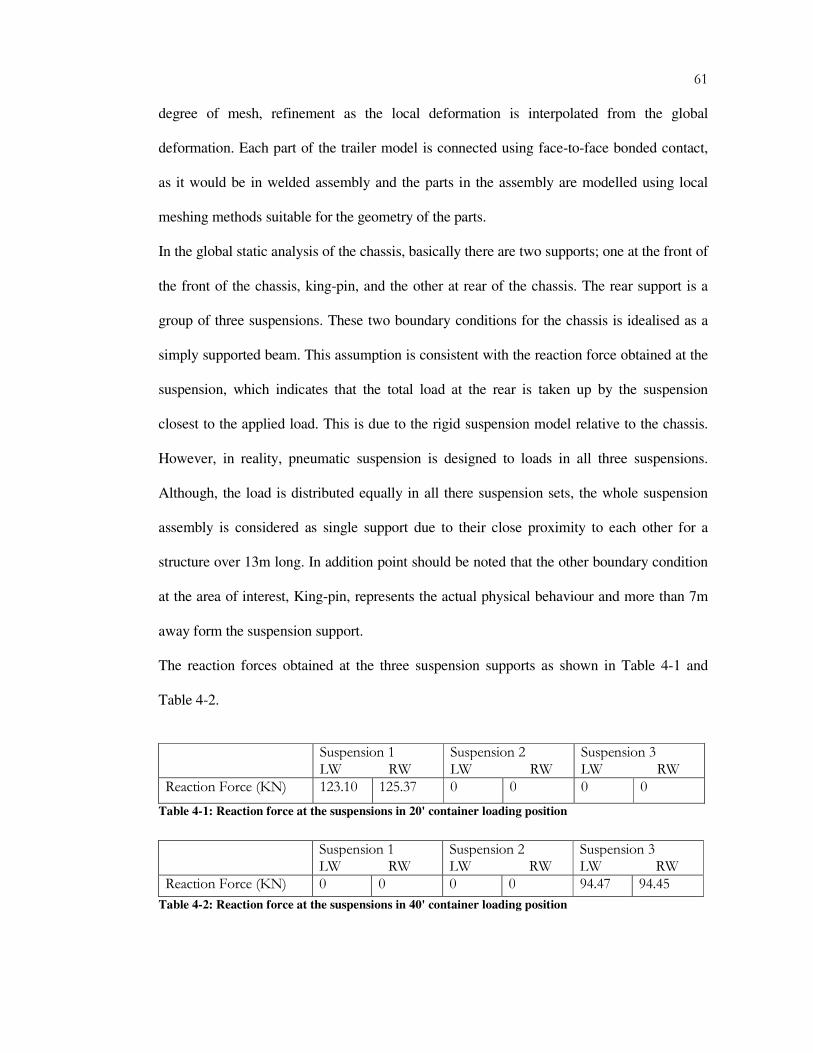
61

degree of mesh, refinement as the local deformation is interpolated from the global

deformation. Each part of the trailer model is connected using face-to-face bonded contact,

as it would be in welded assembly and the parts in the assembly are modelled using local

meshing methods suitable for the geometry of the parts.

In the global static analysis of the chassis, basically there are two supports; one at the front of

the front of the chassis, king-pin, and the other at rear of the chassis. The rear support is a

group of three suspensions. These two boundary conditions for the chassis is idealised as a

simply supported beam. This assumption is consistent with the reaction force obtained at the

suspension, which indicates that the total load at the rear is taken up by the suspension

closest to the applied load. This is due to the rigid suspension model relative to the chassis.

However, in reality, pneumatic suspension is designed to loads in all three suspensions.

Although, the load is distributed equally in all there suspension sets, the whole suspension

assembly is considered as single support due to their close proximity to each other for a

structure over 13m long. In addition point should be noted that the other boundary condition

at the area of interest, King-pin, represents the actual physical behaviour and more than 7m

away form the suspension support.

The reaction forces obtained at the three suspension supports as shown in Table 4-1 and

Table 4-2.

Suspension 1 LW RW

Suspension 2 LW RW

Suspension 3 LW RW

Reaction Force (KN) 123.10 125.37 0 0 0 0

Table 4-1: Reaction force at the suspensions in 20' container loading position

Suspension 1 LW RW

Suspension 2 LW RW

Suspension 3 LW RW

Reaction Force (KN) 0 0 0 0 94.47 94.45

Table 4-2: Reaction force at the suspensions in 40' container loading position

62

Based on the reaction forces obtained in the global static analysis, the turning moment is

applied at the first axle in the case of 20' “worst case” container position, while it is applied

to the third axle in the case of 40' “worst case” container position. The turning moment is

calculated from the normal force acting at suspension support (reaction force) and the

contact surface area of the tyres in laden condition, as shown in the Figure 4-6 below. The

contact area of 245mm x 510mm for the tyres is taken from company records, which is

245mm x 510mm for the tyres normally used for the trailer. The turning moment at the

support is calculated as follows and tabulated in Table 4-3.

FM δρδ *= (4-3)

AM δσρδ **=⇒ (4-4)

maxρ

M

245

510

Figure 4-6: showing the contact surface area for twin tyre for calculating the turning moment.

63

Assuming the moment arm and stress is constant at the contact surface and integrating the

equation (4-4) on both sides gives:

AAM δσρδσρδ ∫ ∫∫ ≈= *** max (4-5)

NAM **** maxmax µρσρ =≈ (4-6)

Substituting

=

A

N*µσ in the above equation

(4-7)

NM **max µρ≈ (4-8)

Where, M = turning moment at the wheel

msxρρ ≈ = moment arm for tyre ground contact surface area (constant)

N = Normal force on the wheels

=σ Stress at the contact surface area (constant)

µ = coefficient of friction for rubber on asphalt (dry) = 1.2 [40]

20’ loading condition-suspension 1 LW RW

40’ loading condition-suspension 3 LW RW

Moment in KN-mm 41789.98 42560.61 32070.68 32063.89 Table 4-3: calculated turning moment at the supports in 20' and 40' container position.

The purpose of the global analysis is to identify the region of highest stresses as shown in

Figure 4-7 to Figure 4-10 for the loading conditions investigated in this project. As a result of

global analysis very high stress are identified at the King-pin region, which is the area of

interest. The high stresses in this region are due to the stress raiser, as the global CAD model

does not represent a very accurate geometry at the kingpin region. Therefore, it is required to

model the geometry with accurate details including weldment. The analysis of the detailed

64

model of the kingpin region using sub-modeling analysis is explained in the following

section. The results obtained in the global analysis is saved and further used in the sub-

modeling analysis of the king-pin region.

Figure 4-7: showing the stress distribution in the global model in 20'container loading position

65

Figure 4-8: showing the stress distribution in the global model in 40'container loading position

Figure 4-9: showing the stress distribution in the global model for “worst case” in 20'container loading

position

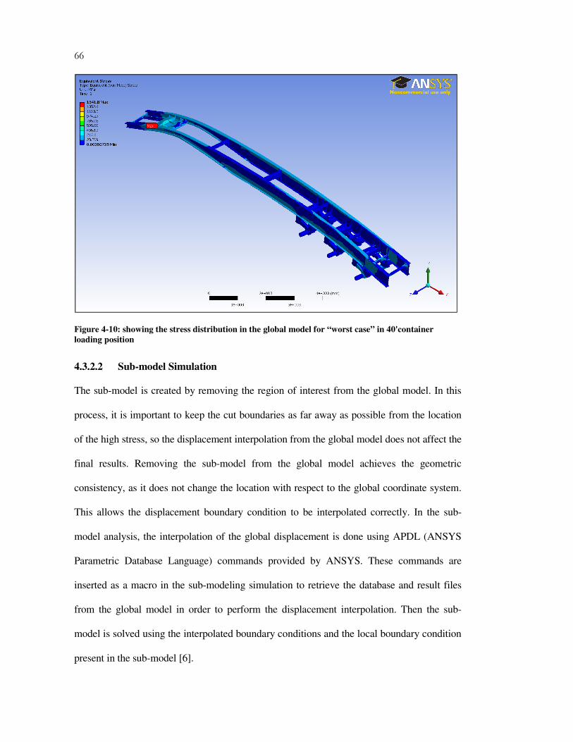
66

Figure 4-10: showing the stress distribution in the global model for “worst case” in 40'container

loading position

4.3.2.2 Sub-model Simulation

The sub-model is created by removing the region of interest from the global model. In this

process, it is important to keep the cut boundaries as far away as possible from the location

of the high stress, so the displacement interpolation from the global model does not affect the

final results. Removing the sub-model from the global model achieves the geometric

consistency, as it does not change the location with respect to the global coordinate system.

This allows the displacement boundary condition to be interpolated correctly. In the sub-

model analysis, the interpolation of the global displacement is done using APDL (ANSYS

Parametric Database Language) commands provided by ANSYS. These commands are

inserted as a macro in the sub-modeling simulation to retrieve the database and result files

from the global model in order to perform the displacement interpolation. Then the sub-

model is solved using the interpolated boundary conditions and the local boundary condition

present in the sub-model [6].

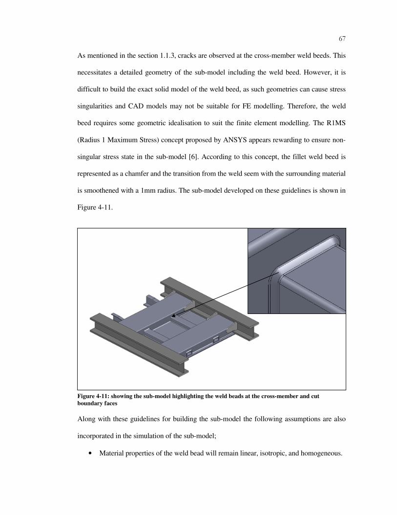
67

As mentioned in the section 1.1.3, cracks are observed at the cross-member weld beeds. This

necessitates a detailed geometry of the sub-model including the weld beed. However, it is

difficult to build the exact solid model of the weld beed, as such geometries can cause stress

singularities and CAD models may not be suitable for FE modelling. Therefore, the weld

beed requires some geometric idealisation to suit the finite element modelling. The R1MS

(Radius 1 Maximum Stress) concept proposed by ANSYS appears rewarding to ensure non-

singular stress state in the sub-model [6]. According to this concept, the fillet weld beed is

represented as a chamfer and the transition from the weld seem with the surrounding material

is smoothened with a 1mm radius. The sub-model developed on these guidelines is shown in

Figure 4-11.

Along with these guidelines for building the sub-model the following assumptions are also

incorporated in the simulation of the sub-model;

• Material properties of the weld bead will remain linear, isotropic, and homogeneous.

Figure 4-11: showing the sub-model highlighting the weld beads at the cross-member and cut

boundary faces

68

• Weld and HAZ (Heat Affected Zone) have the same properties as the base metal.

• Full penetration of the weld is attained.

• No residual stress due to forming will be included.

The sub-model is then meshed with fine elements to accurately represent the geometry. In

this sub-model, very fine mesh discretization was obtained using the “sphere of influence”

method available in ANSYS workbench platform, which allows local mesh control at the

area of interest in the sub-model [31]. The sub-model meshed using the “sphere of influence”

mesh control is shown in Figure 4-12 below.

Figure 4-12: showing the submodel mesh detail using the “sphere of influence” mesh control

4.3.3 Simulation results and discussion

The sub-modeling analysis of the critical area has confirmed the presence of the high stresses

in that region. This correlated well with the location where cracks have been observed on the

actual chassis, as shown in the Figure 1-2. The maximum principal stresses obtained in the

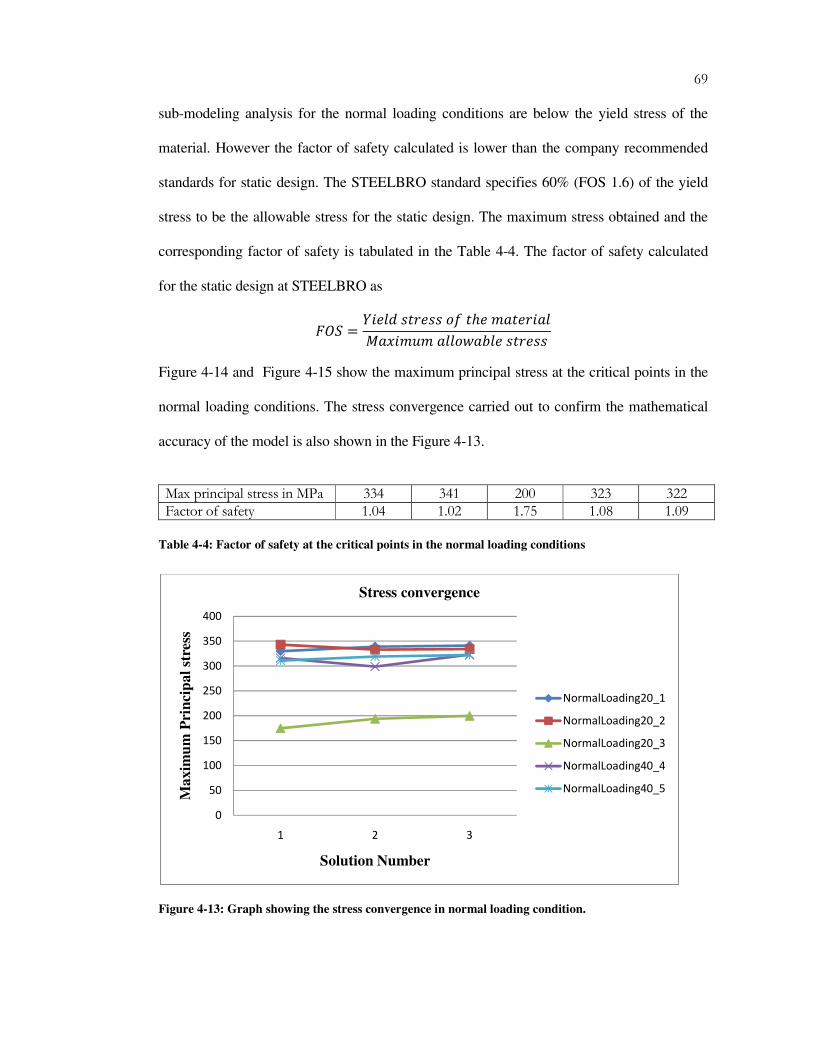
69

sub-modeling analysis for the normal loading conditions are below the yield stress of the

material. However the factor of safety calculated is lower than the company recommended

standards for static design. The STEELBRO standard specifies 60% (FOS 1.6) of the yield

stress to be the allowable stress for the static design. The maximum stress obtained and the

corresponding factor of safety is tabulated in the Table 4-4. The factor of safety calculated

for the static design at STEELBRO as

� = [?<B\��]<��^_�ℎ<@A�<]?AB5A�?@a@ABB^=AbB<��]<��

Figure 4-14 and Figure 4-15 show the maximum principal stress at the critical points in the

normal loading conditions. The stress convergence carried out to confirm the mathematical

accuracy of the model is also shown in the Figure 4-13.

Max principal stress in MPa 334 341 200 323 322 Factor of safety 1.04 1.02 1.75 1.08 1.09

Table 4-4: Factor of safety at the critical points in the normal loading conditions

Figure 4-13: Graph showing the stress convergence in normal loading condition.

0

50

100

150

200

250

300

350

400

1 2 3

Maxim

um

Pri

nci

pa

l st

ress

Solution Number

Stress convergence

NormalLoading20_1

NormalLoading20_2

NormalLoading20_3

NormalLoading40_4

NormalLoading40_5

70

The sub-modeling analysis of the “worst case” service condition showed that the maximum

principal stresses exceeds the yield stress of the material, which means either the structure

will fail or plastic deformation will occur. The analysis performed on the trailer uses only

“elastic model”, which indicates that any value beyond the elastic region will be a linear

estimate at the critical point and may not be an actual value. More accurate results at this

situation would require modelling trailer as an “elasto-plastic” model. However, determining

the stress in the plastic zone is not the aim of this analysis, as the main objective of this

research is to determine the causes of the failure and redesign the component to reduce the

maximum stresses below the failure criteria, which is 60% of the yield stress. The Figure

4-16 and Figure 4-17 shows the maximum stresses for the “worst case” service conditions.

Figure 4-14: showing the critical maximum principal stress at the rub-plate cross- member for 20’

loading condition

71

Figure 4-15: showing the critical maximum principal stress at the rub-plate cross- member for 40’

loading condition

Figure 4-16: showing the critical stress more than the yield stress of the material in the “worst case”

20' container position.

72

Figure 4-17: showing the critical stress more than the yield stress of the material in the “worst case”

40' container position.

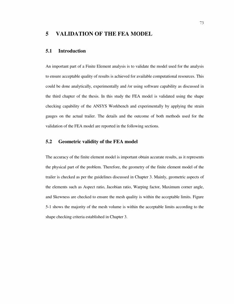
73

5 VALIDATION OF THE FEA MODEL

5.1 Introduction

An important part of a Finite Element analysis is to validate the model used for the analysis

to ensure acceptable quality of results is achieved for available computational resources. This

could be done analytically, experimentally and /or using software capability as discussed in

the third chapter of the thesis. In this study the FEA model is validated using the shape

checking capability of the ANSYS Workbench and experimentally by applying the strain

gauges on the actual trailer. The details and the outcome of both methods used for the

validation of the FEA model are reported in the following sections.

5.2 Geometric validity of the FEA model

The accuracy of the finite element model is important obtain accurate results, as it represents

the physical part of the problem. Therefore, the geometry of the finite element model of the

trailer is checked as per the guidelines discussed in Chapter 3. Mainly, geometric aspects of

the elements such as Aspect ratio, Jacobian ratio, Warping factor, Maximum corner angle,

and Skewness are checked to ensure the mesh quality is within the acceptable limits. Figure

5-1 shows the majority of the mesh volume is within the acceptable limits according to the

shape checking criteria established in Chapter 3.

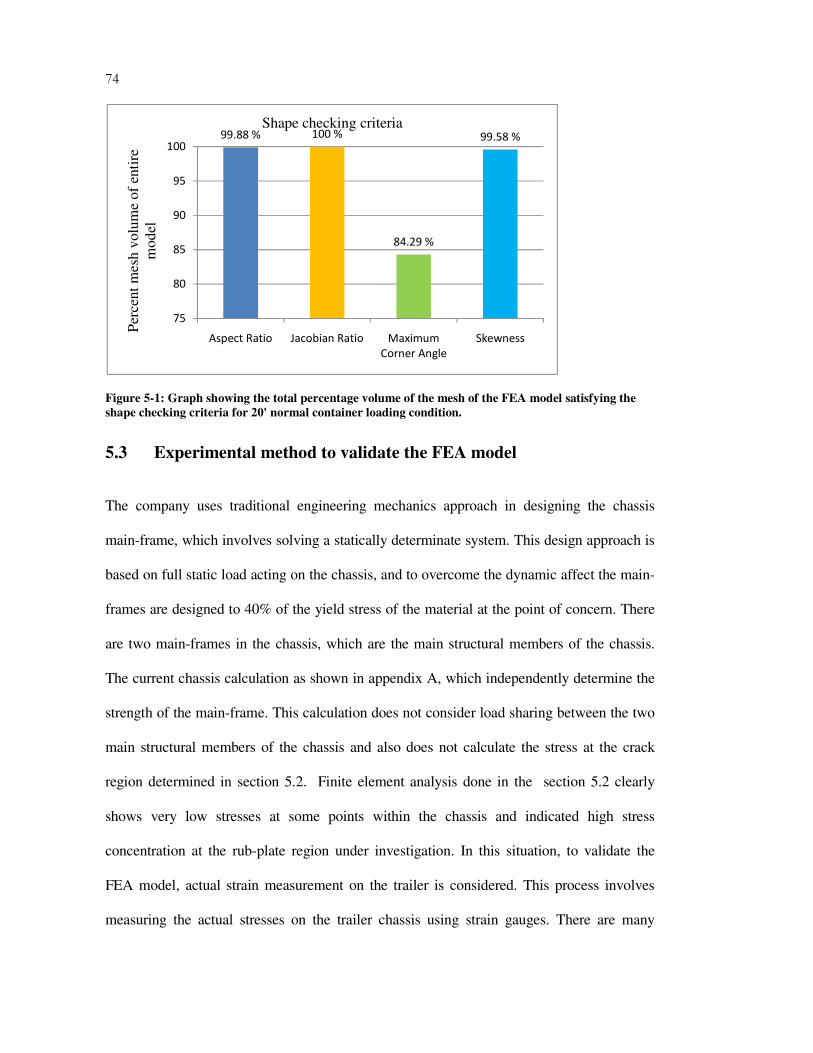
74

Figure 5-1: Graph showing the total percentage volume of the mesh of the FEA model satisfying the

shape checking criteria for 20' normal container loading condition.

5.3 Experimental method to validate the FEA model

The company uses traditional engineering mechanics approach in designing the chassis

main-frame, which involves solving a statically determinate system. This design approach is

based on full static load acting on the chassis, and to overcome the dynamic affect the main-

frames are designed to 40% of the yield stress of the material at the point of concern. There

are two main-frames in the chassis, which are the main structural members of the chassis.

The current chassis calculation as shown in appendix A, which independently determine the

strength of the main-frame. This calculation does not consider load sharing between the two

main structural members of the chassis and also does not calculate the stress at the crack

region determined in section 5.2. Finite element analysis done in the section 5.2 clearly

shows very low stresses at some points within the chassis and indicated high stress

concentration at the rub-plate region under investigation. In this situation, to validate the

FEA model, actual strain measurement on the trailer is considered. This process involves

measuring the actual stresses on the trailer chassis using strain gauges. There are many

99.88 % 100 %

84.29 %

99.58 %

75

80

85

90

95

100

Aspect Ratio Jacobian Ratio Maximum

Corner Angle

Skewness

Per

cen

t m

esh

vo

lum

e o

f en

tire

mo

del

Shape checking criteria

75

mechanical and electrical methods to measure the strain induced in a structural element.

However, Strain gauges are used in this project due to their ease of use and superior

measuring characteristics. Strain gauges record the mechanical strain induced due to

deformation caused by applied force or loads. These stains could be further converted to

stresses and loads to determine the factor of safety of a structural element or validate a FEA

model, as in this study.

Before proceeding to the application of the strain gauges in this project, it is necessary to

have a good understanding about the relevant engineering terminologies and principals in

context with the strain gauge technology. The following sections provide an overview of the

relevant terminologies discussed in the strain gauging process.

5.3.1 Fundamentals of Strain, stress, and Poisson’s Ratio

External force (P) applied on the body causes the deformation in the elastic material of the

body. As the body undergoes deformation, it develops resistance against the deformation.

Broadly, this resistance to deformation is known as stress (σ), which could either be tensile

or compressive in nature as shown in Figure 5-2. If the force is tensile, the initial length of

material extends by ∆L. while compressive forces contract the initial length of the body by

∆L known as Strain (ε ) and the ratio of the change in length to the initial length is expressed

as follows [32]:

(Tensile)L

L∆=ε

(Compressive)

L

L∆−=ε

=∆ L Change in length

=L Initial length

76

Figure 5-2: Illustrative example showing tensile and compressive force acting on a piece of bar [32].

This strain could be converted to stress using the Hooke’s law, which states that the stress is

proportional to the strain within the elastic limit of the material. Therefore the stress can be

determined by multiplying the corresponding strain with the Elastic Modulus of the material.

The Hooke’s law is expressed as below:

εσ E=

=σ Stress

=E Elastic modulus

=ε Strain

As shown in the above figure, when a tensile force is applied on the piece of bar, it induces

two types of strains in the body; longitudinal strain in the axial direction and transverse strain

in the transverse direction of the body. Both strains can be mathematically expressed as

follows [32]:

=1ε Longitudinal strain = L

L∆±

77

=2ε Transverse strain = D

D∆±

Poison’s ratio is a material property defined as the ratio of the absolute value of the

transverse and the longitudinal strains and mathematically expressed as below:

1

2

ε

εν =

where,

=ν Poisson’s Ratio

5.3.2 Strain gauge and Principal of strain measurement

Two types of strain gauges are used in this project. Basically, the strain gauges are made up

of fine electrical resistance wire or photographically etched metallic foil. As shown in Figure

5-3, the wire or metallic foil is bonded to an insulated surface and connected to the lead

wires. In order to measure strain, the insulated surface is glued onto the test specimen using

non-conductive adhesive. When the test specimen undergoes any deformation, a

corresponding change in the electrical resistance occurs in the wire or foil. This change in the

electrical resistance is recorded as the strain in the test specimen at the point of application of

the strain gauge. Linear strain gauges determine the strain in a single direction, while Tri-

axial strain gauge rosettes are able to determine the full state of strain at a point via equation

5-1, which includes the Young’s modulus and Poisson’s ratio of the material. Generally, the

tri-axial rosette gauges are used if the direction of the principal axis is uncertain [33]. The

strain gauge rosette used in this project is shown in Figure 5-4.

78

Figure 5-3: Schematic of a general-purpose foil strain gauge (Kyowa, Japan), these were used for the

stress measurement on the Mainframe flanges [33].

Figure 5-4: Schematic of a 3-element rosette strain gauge (Tokyo Sokki Kenkyujo, Japan), these were

used for the stress measurement of the Rub-plate cross-member ‘hot spot’ areas [33].

Maximum principal stress: ( ) ( ){ }

−+−

++

+

+=

2

32

2

3121 2

1

1

12εεεε

νν

εεE (5-1)

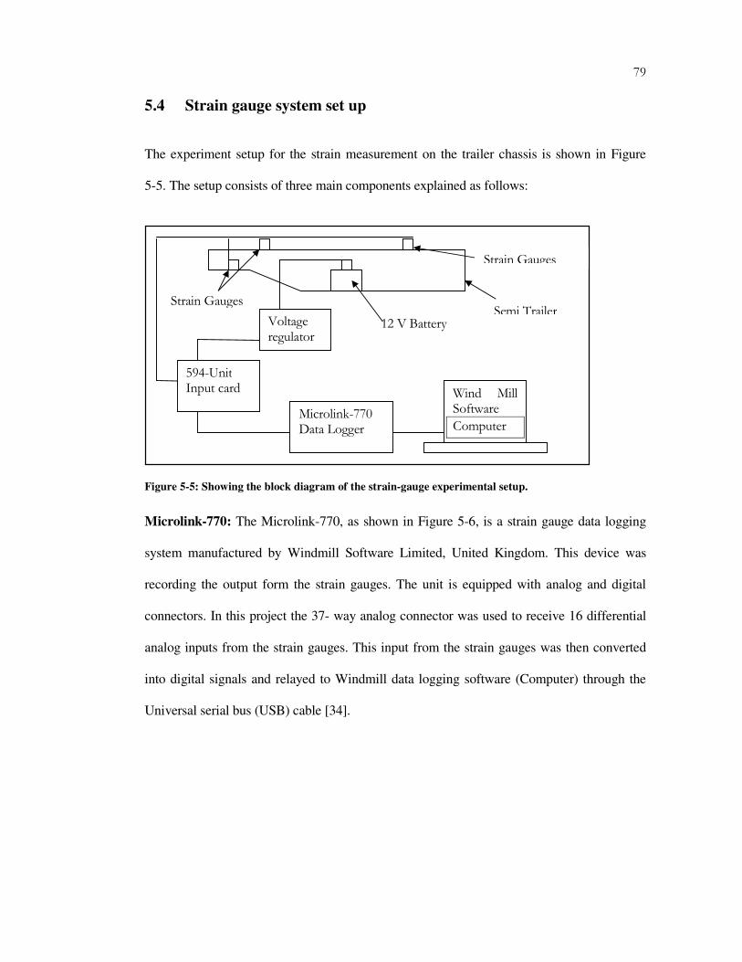
79

5.4 Strain gauge system set up

The experiment setup for the strain measurement on the trailer chassis is shown in Figure

5-5. The setup consists of three main components explained as follows:

Figure 5-5: Showing the block diagram of the strain-gauge experimental setup.

Microlink-770: The Microlink-770, as shown in Figure 5-6, is a strain gauge data logging

system manufactured by Windmill Software Limited, United Kingdom. This device was

recording the output form the strain gauges. The unit is equipped with analog and digital

connectors. In this project the 37- way analog connector was used to receive 16 differential

analog inputs from the strain gauges. This input from the strain gauges was then converted

into digital signals and relayed to Windmill data logging software (Computer) through the

Universal serial bus (USB) cable [34].

Microlink-770 Data Logger

Wind Mill Software

Computer

12 V Battery

Strain Gauges Semi Trailer

594-Unit Input card

Strain Gauges

Voltage regulator

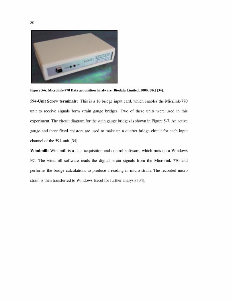
80

Figure 5-6: Microlink-770 Data acquisition hardware (Biodata Limited, 2000, UK) [34].

594-Unit Screw terminals: This is a 16 bridge input card, which enables the Micrlink-770

unit to receive signals form strain gauge bridges. Two of these units were used in this

experiment. The circuit diagram for the stain gauge bridges is shown in Figure 5-7. An active

gauge and three fixed resistors are used to make up a quarter bridge circuit for each input

channel of the 594-unit [34].

Windmill: Windmill is a data acquisition and control software, which runs on a Windows

PC. The windmill software reads the digital strain signals from the Microlink 770 and

performs the bridge calculations to produce a reading in micro strain. The recorded micro

strain is then transferred to Windows Excel for further analysis [34].

81

Figure 5-7: Circuit diagram of the quarter bridge connection used in the 594-Unit screw terminal [34].

5.5 Experimental procedure

The strain gauges were applied on the selected points on the trailer and connected to the

electronic set up as explained in the section 5.4. In an anticipation of human errors and

technical problems, 16 strain gauges were applied on the chassis. Eight of the strain gauges

were Rosette gauges attached to the selected points at the rub-plate cross-member region,

which is the failure region. As shown in Figure 5-8, each Rosette strain gauge consists of 3

gauges stacked on top of each other and these gauges occupied 24 channels in the 594-Unit

screw terminal. The remaining eight linear strain gauges were applied on top and bottom

flange of the left hand side mainframe of the chassis. The linear strain gauge application

points were selected based on the analytically calculated results, as the points could be

compared with strain gauge readings. Figure 5-8 shows the electronic set up of the

instruments at the rub-plate region of the trailer.

Active strain gauge

3 Fixed resistors

82

The following two testing scenarios were performed on the trailer to obtain the strain gauge

readings.

• Case 1 – Strain gauge data recorded during normal loading/unloading ( full load )in

static condition for 20’ container position (Figure 5-9)

• Case 2 – Strain gauge data collected during normal loading/ unloading (full load) in

static condition for 40’ container position (Figure 5-10)

Figure 5-8: Complete setup of the strain gauge system at the chassis rub-plate, the enlarged view

of one of the Rosette strain gauge is shown at the bottom left corner of the picture.

83

Figure 5-9: The 20' full load testing position at STEELBRO yard.

Figure 5-10: The 40' full load testing position at STEELBRO yard.

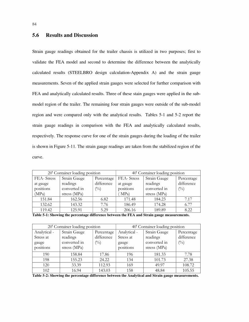
84

5.6 Results and Discussion

Strain gauge readings obtained for the trailer chassis is utilized in two purposes; first to

validate the FEA model and second to determine the difference between the analytically

calculated results (STEELBRO design calculation-Appendix A) and the strain gauge

measurements. Seven of the applied strain gauges were selected for further comparison with

FEA and analytically calculated results. Three of these stain gauges were applied in the sub-

model region of the trailer. The remaining four strain gauges were outside of the sub-model

region and were compared only with the analytical results. Tables 5-1 and 5-2 report the

strain gauge readings in comparison with the FEA and analytically calculated results,

respectively. The response curve for one of the strain gauges during the loading of the trailer

is shown in Figure 5-11. The strain gauge readings are taken from the stabilized region of the

curve.

20' Container loading position 40' Container loading position FEA- Stress at gauge positions (MPa)

Strain Gauge readings converted in stress (MPa)

Percentage difference (%)

FEA- Stress at gauge positions ( MPa)

Strain Gauge readings converted in stress (MPa)

Percentage difference (%)

151.84 162.56 6.82 171.48 184.23 7.17 132.62 143.32 7.76 186.49 174.28 6.77 119.42 125.91 5.29 206.16 189.89 8.22

Table 5-1: Showing the percentage difference between the FEA and Strain gauge measurements.

20' Container loading position 40' Container loading position Analytical - Stress at gauge positions

Strain Gauge readings converted in stress (MPa)

Percentage difference (%)

Analytical - Stress at gauge positions

Strain Gauge readings converted in stress (MPa)

Percentage difference (%)

190 158.84 17.86 196 181.33 7.78 198 155.23 24.22 134 101.73 27.38 120 33.39 112.93 169 49.97 108.72 102 16.94 143.03 158 48.84 105.55

Table 5-2: Showing the percentage difference between the Analytical and Strain gauge measurements.

85

The percentage difference between calculated FEA results and the strain gauge readings at

the cross-member region is between 5 to 9 % within the sub-model cross-member region of

the trailer. Considering the level of noise in the system due to diesel engine mounted on the

trailer, this is a good level of correlation between the FEA and experimental values. On the

other hand, comparison with the analytical values showed that the percentage difference was

large, especially at the strain gauges mounted at the rear end of the trailer. This large

percentage difference could be due to the simplification done in the analytical calculation for

the mainframe.

Figure 5-11: Showing the nature of the curve at a strain gauge location in 20' container loading

position. The maximum value of 158.84 MPa is recorded in the stable region of the graph.

-180.00

-160.00

-140.00

-120.00

-100.00

-80.00

-60.00

-40.00

-20.00

0.00

20.00

1

44

87

13

0

17

3

21

6

25

9

30

2

34

5

38

8

43

1

47

4

51

7

56

0

60

3

64

6

68

9

73

2

77

5

81

8

86

1

90

4

Str

ess

(M

Pa

)

Time (s)

Strain gauge data

86

6 FEA: REVISED DESIGN

6.1 Introduction

The aim of this study is to determine the cause of the observed failure, so that the component

can be redesigned to resist cracking. The analysis of Chapter 4 showed that “worst case”

service condition could be the cause of the failure, however if it is assumed that the trailer

never come across the “worst case” service condition, then the study must focus on normal

loading/unloading conditions. Even though the stresses determined in the static analysis are

below the yield stress, the phenomenon of metal fatigue could cause the failure under the

cyclic loading conditions. Therefore, this chapter further investigates the effect of cyclic

loading on the critical region identified in the static analysis for normal loading/unloading

conditions.

6.2 Fatigue analysis of the current design

Generally, the objective of fatigue analysis is to estimate the number of repeated cycles of

loading a component may experience in it’s life time so that the component can be designed

to withstand more than the desired number of loading cycles. For the fatigue analysis of the

current design, it is important to understand the nomenclature associated with the cyclic

loading, as shown in Figure 6-1.

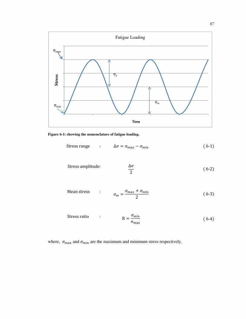
87

Figure 6-1: showing the nomenclature of fatigue loading.

Stressrange: ∆� = ���� − ���� (6-1)

Stressamplitude: ∆�2 (6-2)

Meanstress: �� = ���� + ����2 (6-3)

Stressratio: R = ����σnop (6-4)

where, ���� and ���� are the maximum and minimum stress respectively.

Str

ess

Time

Fatigue Loading

σmax

σmin

σm

σa

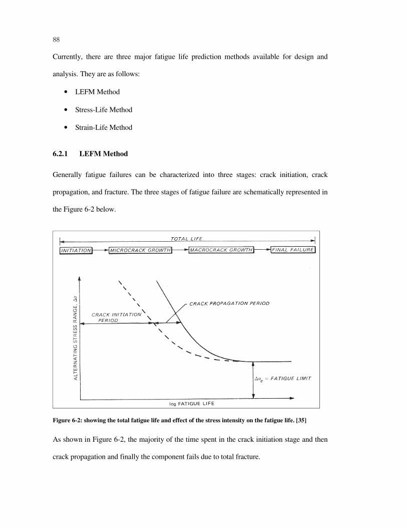
88

Currently, there are three major fatigue life prediction methods available for design and

analysis. They are as follows:

• LEFM Method

• Stress-Life Method

• Strain-Life Method

6.2.1 LEFM Method

Generally fatigue failures can be characterized into three stages: crack initiation, crack

propagation, and fracture. The three stages of fatigue failure are schematically represented in

the Figure 6-2 below.

Figure 6-2: showing the total fatigue life and effect of the stress intensity on the fatigue life. [35]

As shown in Figure 6-2, the majority of the time spent in the crack initiation stage and then

crack propagation and finally the component fails due to total fracture.

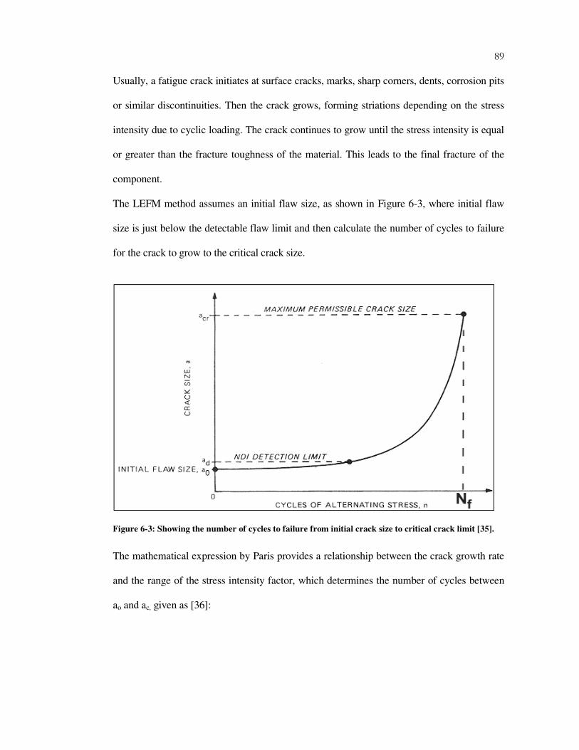
89

Usually, a fatigue crack initiates at surface cracks, marks, sharp corners, dents, corrosion pits

or similar discontinuities. Then the crack grows, forming striations depending on the stress

intensity due to cyclic loading. The crack continues to grow until the stress intensity is equal

or greater than the fracture toughness of the material. This leads to the final fracture of the

component.

The LEFM method assumes an initial flaw size, as shown in Figure 6-3, where initial flaw

size is just below the detectable flaw limit and then calculate the number of cycles to failure

for the crack to grow to the critical crack size.

Figure 6-3: Showing the number of cycles to failure from initial crack size to critical crack limit [35].

The mathematical expression by Paris provides a relationship between the crack growth rate

and the range of the stress intensity factor, which determines the number of cycles between

ao and ac, given as [36]:

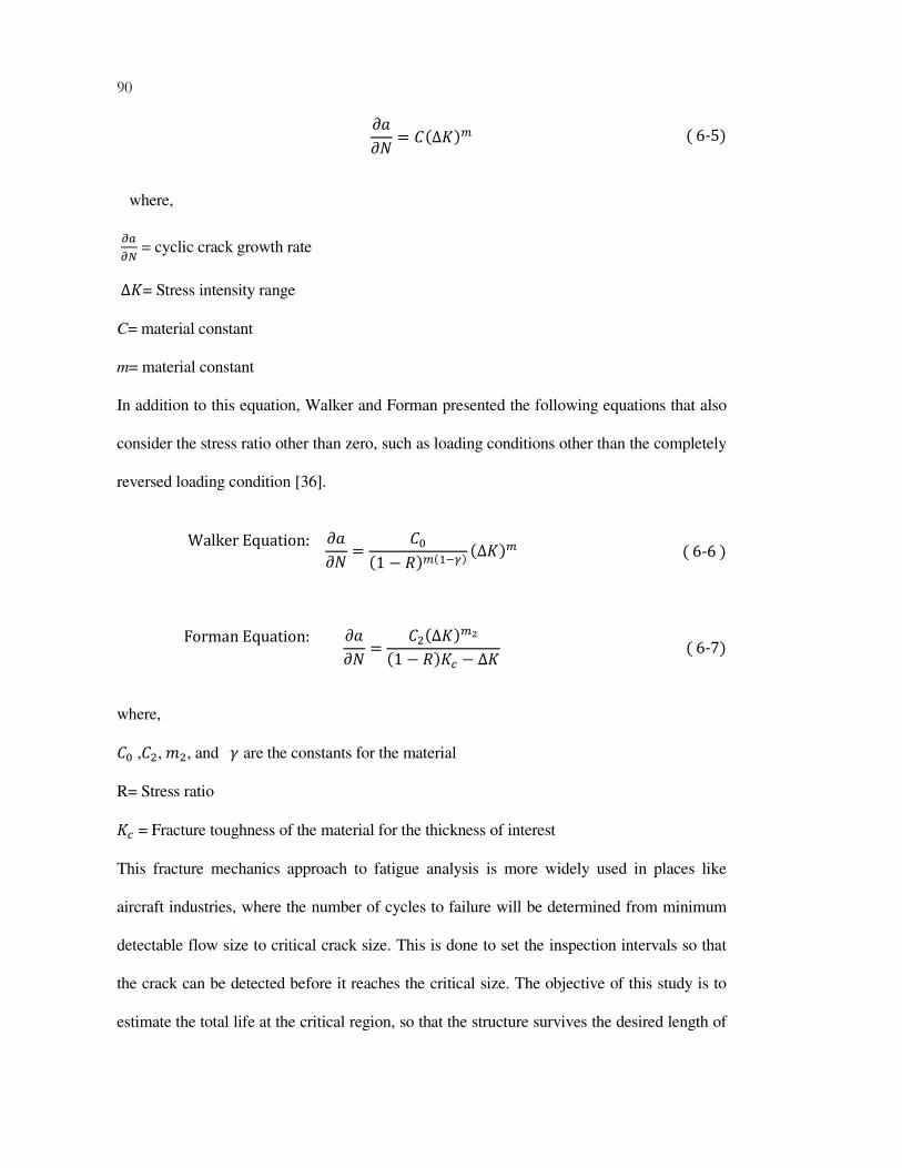
90

qAq� = C(∆�)� (6-5)

where,

r�rs = cyclic crack growth rate

∆�= Stress intensity range

C= material constant

m= material constant

In addition to this equation, Walker and Forman presented the following equations that also

consider the stress ratio other than zero, such as loading conditions other than the completely

reversed loading condition [36].

WalkerEquation: qAq� = Cx(1 − �)�($yz) (∆�)� (6-6)

FormanEquation: qAq� = C%(∆�)�{

(1 − �)� − ∆� (6-7)

where,

Cx ,C%,@%, and | are the constants for the material

R= Stress ratio

� = Fracture toughness of the material for the thickness of interest

This fracture mechanics approach to fatigue analysis is more widely used in places like

aircraft industries, where the number of cycles to failure will be determined from minimum

detectable flow size to critical crack size. This is done to set the inspection intervals so that

the crack can be detected before it reaches the critical size. The objective of this study is to

estimate the total life at the critical region, so that the structure survives the desired length of

91

time before any further inspection. This is more easily achieved using either stress-life

method or strain-life method, as explained in the following sections.

6.2.2 Stress-Life Method

The Stress-Life method is a traditional approach to analyze metal fatigue based on a stress-

life curve called S-N curve. It is derived from experimental data conducted on a test

specimen. This method was first introduced by German engineer August Wo� ller. This is also

called the “nominal stress” approach as it uses nominal or average stress acting on the

component for the fatigue analysis [36].

Generally, experimental data for a test specimen could be obtained by various fatigue testing

machines depending on the loading condition; for example, R. R. Moore rotating beam

machine is used for applying pure bending by means of weights [37]. Due to statistical

nature of the fatigue, several tests are required to determine the fatigue strength of a material

which eventually produces the S-N curve. Figure 6-4 shows the typical S-N curve for steels

and non-ferrous alloys.

92

Figure 6-4: showing the typical S-N curve for

The S-N curve is usually obtained by plotting the data points on semi

The resulting curve could be fitted by

the stress amplitude and number of cycles to failure

where,

'

fσ = fatigue strength of material

b = fatigue strength exponent

For steels, fatigue failures less than 10

cycle fatigue deals with failures at more than

“knee-bend” can be observed in the graph which indicate

limit” of the material ('

eS ). Beyond this limit the material will

N curve for steel and non-ferrous alloys [35].

N curve is usually obtained by plotting the data points on semi-log or log-log paper.

fitted by mathematical equation as shown below, which relates

the stress amplitude and number of cycles to failure [36].

( )b

ffa N2'σσ =

fatigue failures less than 103 cycles are considered as low cycle fatigue and

s at more than 103 cycles. As shown in Figure 6-4, for steels, a

” can be observed in the graph which indicates the “endurance limit” or

). Beyond this limit the material will not fail for any amount of

log paper.

mathematical equation as shown below, which relates

(6-8)

cycles are considered as low cycle fatigue and high

, for steels, a

or “fatigue

for any amount of

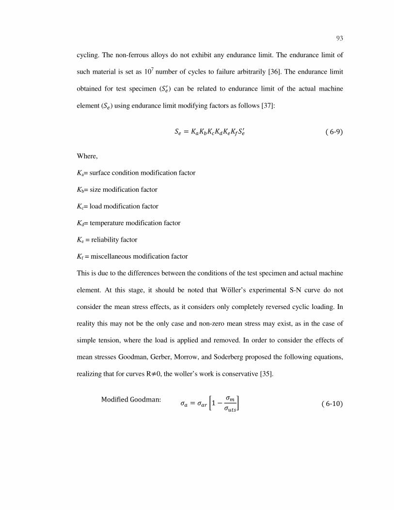
93

cycling. The non-ferrous alloys do not exhibit any endurance limit. The endurance limit of

such material is set as 107

number of cycles to failure arbitrarily [36]. The endurance limit

obtained for test specimen (���) can be related to endurance limit of the actual machine

element (��) using endurance limit modifying factors as follows [37]:

�� = ���}� �~������� (6-9)

Where,

Ka= surface condition modification factor

Kb= size modification factor

Kc= load modification factor

Kd= temperature modification factor

Ke = reliability factor

Kf = miscellaneous modification factor

This is due to the differences between the conditions of the test specimen and actual machine

element. At this stage, it should be noted that Wo� ller’s experimental S-N curve do not

consider the mean stress effects, as it considers only completely reversed cyclic loading. In

reality this may not be the only case and non-zero mean stress may exist, as in the case of

simple tension, where the load is applied and removed. In order to consider the effects of

mean stresses Goodman, Gerber, Morrow, and Soderberg proposed the following equations,

realizing that for curves R≠0, the woller’s work is conservative [35].

ModifiedGoodman: �� = ��+ F1 − ���'�(J (6-10)

94

Gerber: �� = ��+ �1 − � ���'�(�%� (6-11)

Soderberg: �� = ��+ �1 − ���#(� (6-12)

Morrow: �� = ��+ �1 − ����� � (6-13)

Where,

�� = mean stress

�'�( = ultimate tensile strength

�#( = yield strength

�� = fatigue strength when �� ≠ 0

��+ = fatigue strength in fully reversed loading condition, when �� = 0

Out of all the above equations, Soderberg is considered to be most conservative, as it uses

the yield stress to be the failure criteria. The Gerber equation more closely fits the

experimental data where mean tensile stress is involved and is not suitable for compressive

mean stress. Similarly the Goodman equation best fit the data for low-ductile material like

high tensile steel or brittle material and the equation modified by Morrow seems to have the

best correlation with ductile material experimental data when the true fracture stress is in

tension where a material constant ( ���) is considered as the failure criteria [36]. Therefore,

proper selection of the mean stress equation depends on many variables.

95

As mentioned previously, the Stress-Life approach is mainly based on experimental data. It

is reasonable to use this method to estimate fatigue life, for estimating fatigue life, if the S-N

curve or experimental fatigue data exist for the material. This method is accurate for high

cycle fatigue, where the fatigue life is dominated by elastic strain of the component.

In this project ANSYS Workbench FEA fatigue module has been used to estimate the fatigue

life of the component. The FEA fatigue module requires an S-N curve, which is not readily

available for the trailer material to be used as a input to calculate the fatigue life in the stress-

life method. Although the S-N curve could be produced analytically using the limited

experimental data available for the material, the process could be more complex and it would

be easier to use strain-life method, which would need only fatigue parameters to estimate

fatigue life in ANSYS Workbench fatigue software. The Strain-Life method used to estimate

the fatigue life at the critical location of the component is explained in the next section.

96

6.2.3 Strain-Life Method

Fatigue cracks normally start at local discontinuities. Strain-Life fatigue analysis considers

deformation as a cumulative effect of elastic and plastic strains. This method is very

successful in defining shorter life span of components, where plasticity causes the majority

of the damage. The method can also be used for high cycle fatigue problems as it considers

the elastic and plastic strain responsible for fatigue failure. Strain-Life method can thus

considered as comprehensive approach to deal with the fatigue problem [36].

This strain based approach estimates local stress and strain at the crack region. Most

importantly, it considers the local yielding at the crack region and uses cyclic stress-strain

and strain-life curves in the fatigue life estimation process. For this study, the strain-life

curve shown in Figure 6-5 was constructed in ANSYS fatigue module using previously

published fatigue properties of the trailer material [29].

Figure 6-5 shows elastic, plastic, and total strain components. The total strain is

mathematically represented as follows [35]:

∈�=∈��+∈.� (6-14)

Where, ∈��= elastic strain amplitude, ∈.�= plastic strain amplitude

The elastic and plastic strain lines in the strain-life curve are fitted with following equations

respectively [35]:

∈��= ��� = ���� �2���} (6-15)

97

∈.�= !���2��� (6-16)

Where c = fatigue ductility exponent, E = Young’s modulus.

Figure 6-5: The strain life curve constructed in ANSYS using fatigue material properties.

According to the Coffin-Manson relation, when the elastic and plastic equations are

combined, the total strain can be related to total life. The Coffin-Manson relation is presented

as below [35]:

∈�=���� �2���} + !���2��� (6-17)

Similarly, for cyclic stress-strain curve, the Ramberg-Osgood equation can be presented as

follows [35]:

98

∈�= ��� + ������$�� (6-18)

Here total strain amplitude is the sum of elastic and plastic strains, �� is strain hardening

coefficient, and �� is the strain hardening exponent.

Equations 6.17 and 6.18 can be defined using six parameters; four strain-life material

properties and two cyclic stress-strain material properties. Given these fatigue material

properties, the ANSYS Workbench fatigue module can construct the strain-life curve and

cyclic stress strain curve for estimating the fatigue life.

As mentioned before, the strain-life equations uses elastic and plastic strain inputs to

calculate fatigue life. This collective approach can lead to a lengthy finite element simulation

to determine the total response. If the total life is dominated by elastic strain, the time spent

on plastic deformation analysis will not provide any significant result. Therefore ANSYS

fatigue module assumes nominal elastic response and then uses Neuber’s equation to relate

local stress/strain to nominal stress/strain at the critical area. [38].

Neuber’s rule used in ANSYS is presented below:

∈ � = ��%<� (6-19)

Where,

∈ = total local strain

� = local stress

S = nominal elastic stress

�� = elastic stress concentration factor

e = nominal elastic strain

99

The ANSYS fatigue module simultaneously solves the above equation along with Ramberg-

Osgood cyclic strain equation to calculate the total response at the local region using only the

elastic strain. In the above calculation, ANSYS sets the value of Kt as 1, assuming a

perfectly refined mesh of the component [38]. It is therefore necessary to achieve the best

possible stress convergence in the static finite element analysis at the region of fatigue

interest before the fatigue analysis is carried out.

In order to perform the fatigue analysis using strain-life method, two decisions need to be

made to define the fatigue simulation in ANSYS Workbench fatigue module. First the type

of cyclic loading applied on the structure must be identified. In this study, only the container

loading/unloading scenario is considered. In this case a constant load applied and removed.

This could be identified as constant amplitude loading. This is a simple bending load, which

does not change the direction of the principal stress axis. Therefore it could further be

identified as proportional loading and collectively this scenario could be explained as

constant amplitude proportional loading, where the load applied once and then removed ( the

load fluctuates between maximum constant value and zero). As this loading is analyzed as

proportional loading, only a single set of maximum principal stress from the static finite

element results are fed to fatigue module to estimate the fatigue life at the critical location of

the structure [38]. Figure 6-6 showing the graphical representation of the zero based loading

type applied on the trailer.

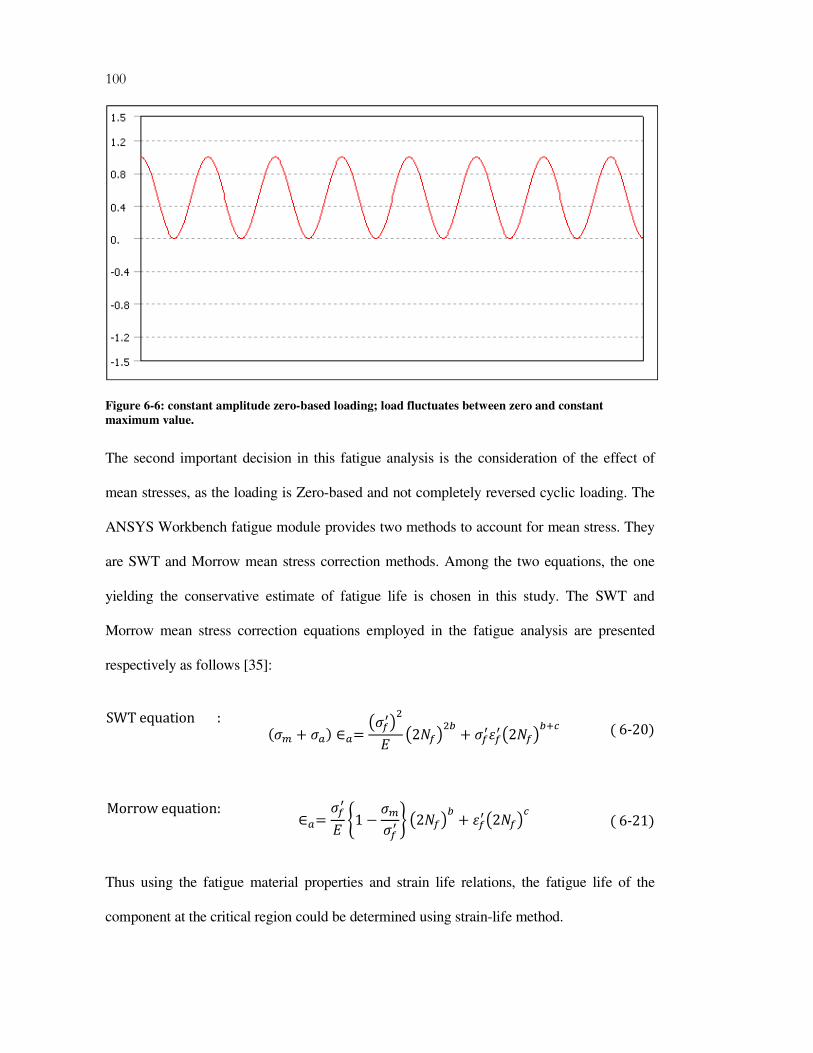
100

Figure 6-6: constant amplitude zero-based loading; load fluctuates between zero and constant

maximum value.

The second important decision in this fatigue analysis is the consideration of the effect of

mean stresses, as the loading is Zero-based and not completely reversed cyclic loading. The

ANSYS Workbench fatigue module provides two methods to account for mean stress. They

are SWT and Morrow mean stress correction methods. Among the two equations, the one

yielding the conservative estimate of fatigue life is chosen in this study. The SWT and

Morrow mean stress correction equations employed in the fatigue analysis are presented

respectively as follows [35]:

SWTequation: (�� + ��) ∈�= �����%� �2���%} + ���!���2���}� (6-20)

Morrowequation: ∈�= ���� �1 − ����� � �2���} + !���2��� (6-21)

Thus using the fatigue material properties and strain life relations, the fatigue life of the

component at the critical region could be determined using strain-life method.

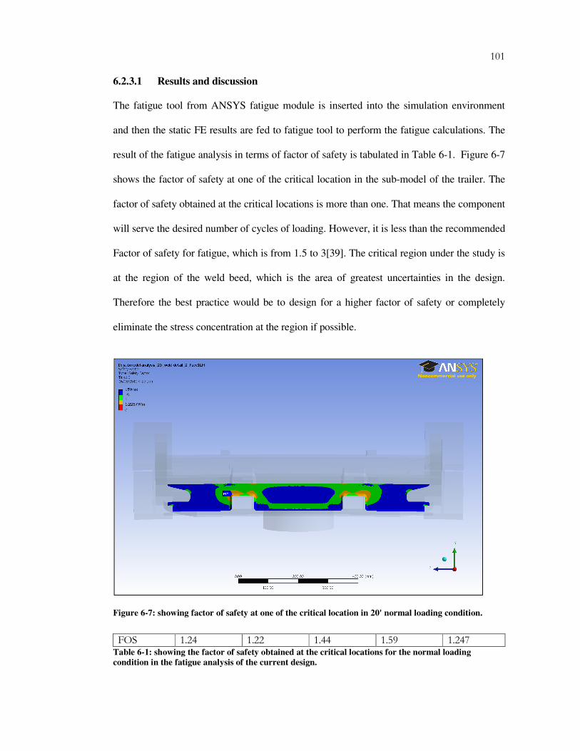
101

6.2.3.1 Results and discussion

The fatigue tool from ANSYS fatigue module is inserted into the simulation environment

and then the static FE results are fed to fatigue tool to perform the fatigue calculations. The

result of the fatigue analysis in terms of factor of safety is tabulated in Table 6-1. Figure 6-7

shows the factor of safety at one of the critical location in the sub-model of the trailer. The

factor of safety obtained at the critical locations is more than one. That means the component

will serve the desired number of cycles of loading. However, it is less than the recommended

Factor of safety for fatigue, which is from 1.5 to 3[39]. The critical region under the study is

at the region of the weld beed, which is the area of greatest uncertainties in the design.

Therefore the best practice would be to design for a higher factor of safety or completely

eliminate the stress concentration at the region if possible.

Figure 6-7: showing factor of safety at one of the critical location in 20' normal loading condition.

FOS 1.24 1.22 1.44 1.59 1.247 Table 6-1: showing the factor of safety obtained at the critical locations for the normal loading

condition in the fatigue analysis of the current design.

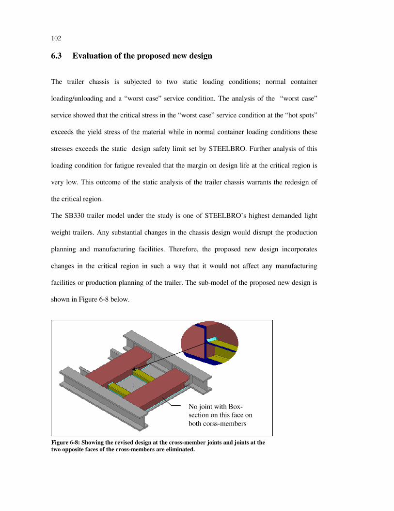
102

6.3 Evaluation of the proposed new design

The trailer chassis is subjected to two static loading conditions; normal container

loading/unloading and a “worst case” service condition. The analysis of the “worst case”

service showed that the critical stress in the “worst case” service condition at the “hot spots”

exceeds the yield stress of the material while in normal container loading conditions these

stresses exceeds the static design safety limit set by STEELBRO. Further analysis of this

loading condition for fatigue revealed that the margin on design life at the critical region is

very low. This outcome of the static analysis of the trailer chassis warrants the redesign of

the critical region.

The SB330 trailer model under the study is one of STEELBRO’s highest demanded light

weight trailers. Any substantial changes in the chassis design would disrupt the production

planning and manufacturing facilities. Therefore, the proposed new design incorporates

changes in the critical region in such a way that it would not affect any manufacturing

facilities or production planning of the trailer. The sub-model of the proposed new design is

shown in Figure 6-8 below.

No joint with Box-

section on this face on

both corss-members

Figure 6-8: Showing the revised design at the cross-member joints and joints at the

two opposite faces of the cross-members are eliminated.

103

Cracks have appeared at the intersection of the rub-plate cross-member and box-section as

shown in Figure 1.1. The finite element analysis has also confirmed the critical spots in the

rub-plate sub-model. Therefore effort has been made to change the joint design at the cross-

member without affecting the structural integrity of the chassis. As shown in the Figure 6-8,

this is achieved by removing the notches in the cross-member for the box-section and

shortening the box-section at both ends. Originally the box-sections were passed through the

cross-members. This is not necessary, as the load transfers from the king-pin through the

rub-plate and cross-member. The proposed new design is subjected to both loading

conditions and results are presented in the Figure 6-10 to Figure 6-13 respectively.

The proposed new design has simplified the joint design at the cross-member region and

eliminated the stress intensity at the stress region, as shown in Figure 6-10 through Figure

6-13. More importantly, this design change is at the drawing level and will not affect any

manufacturing facilities or production planning of the current manufacturing system at the

company.

Figure 6-10: showing the stress distribution on one of the critical locations identified in the old design

for 20' normal loading condition.

104

Figure 6-11: showing the stress distribution on one of the critical locations identified in the old design

for 40' normal loading condition.

Figure 6-12: showing the stress distribution on one of the critical locations identified in the old design

for 20' “worst case” service condition.

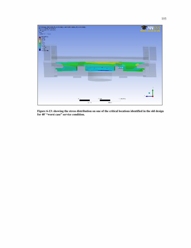
105

Figure 6-13: showing the stress distribution on one of the critical locations identified in the old design

for 40' “worst case” service condition.

106

7 CONCLUSION AND RECOMMENDATIONS

7.1 Conclusion

The structural analysis of the trailer using Finite element analysis is carried out in this study

for two loading conditions; normal loading/unloading condition and a “worst case” loading

condition. These two cases were selected to determine their influence on the cross-member

cracks at the rub-plate region of the trailer. Based on the outcome of the analysis performed

in this study, the following can be concluded.

• If the trailer chassis under goes the “worst case” service condition, it has high

potential to cause damage at the critical region and could be the cause of the failure.

• Static analysis of the normal loading/unloading condition showed that the maximum

stress is below the yield stress. However, the maximum stresses are more than the

recommended static design safety limit.

• Fatigue analysis performed on the normal loading/ unloading condition revealed that

the margin of safety at the critical region against the fatigue loading is low and could

cause failure considering the statistical nature of fatigue failure.

• Finally, a new design is proposed to overcome the potential failure in the static

loading condition for the two loading conditions.

107

7.2 Recommendations

This research was carried to determine the effect of the two loading conditions on an

ongoing problem. In this quest, the above conclusions showed that the trailer chassis

subjected to these loading conditions has a significant effect. However, some

recommendations to be considered in future development of the trailer chassis:

• Fatigue analysis for the normal loading condition showed that the factor of safety is

low at the critical region, even without subjecting the trailer to dynamic loading

conditions. This loading condition could occur for example when trailer is

transporting a loaded container. Therefore fatigue analysis sould be performed

considering the dynamic stress hysteresis to more accurately determine the fatigue

life at the critical region.

• Finite element analysis performed in this research provides global picture of stress

distribution on the chassis. At some locations it can be seen that the stress is very

low, which warrants further investigation for weight to strength ratio optimization of

the chassis. This investigation should also extend to detailed dynamic analysis of the

trailer.

• This thesis is focused on investigating “area of interest”, rub-plate region. Therefore

some assumptions were made at the suspension area and experimental results were

found consistent at the area of interest. However, for future analysis such as dynamic

or complete structural analysis, true characteristics of the suspension assembly

should incorporated in the analysis.

• Fatigue analysis performed using the finite element method should also be validated

by experimental methods.

108

8 REFERENCES

[1] Adams, V., & Askenazi, A. (1999). Building Better Products With Finite Element Analysis.

Santa Fe, USA: OnWard Press.

[2] Cook, R. D., Malkus, D. S., Plesha, M. E., & Witt, R. J. (2002). Concepts And Aplications Of

Finite Element Analysis (4th Edition ed.). USA: John Wiley & Sons, Inc.

[3] Transport Canada. (n.d.). Transport Development Centre:Energy-efficient Light Trailer Engineering

Design (TP 12982E). Retrieved August 28, 2009, from Transport Canada Web site:

www.tc.gc.ca/innovation/tdc/summary/12900/12982e.html

[4] Rahman, A. R., Tamin, M. N., & Kurdi, O. (2008). Stress analysis of heavy duty truck

chassis as a preliminary data for its fatigue life prediction using FEM. Journal Mekanikal ,

76-85.

[5] Kassahum, M. (2008). Static And Dynamic Analysis of a Commercial Vehical With Van Body.

Unpublished Master's Thesis, Addis Ababa University. Ethiopia: Retrieved from

http://etd.aau.edu.et/dspace/handle/123456789/1535.

[6] Wang, E., & Rauch, R. (2008). Fatigue Analysis and Design Optimization of a Trailer

Hitch System. Proceedings of International ANSYS Conference. Germany: Retrived from

http://www.ansys.com/events/proceedings/2008.asp.

[7] Bekah, S. (2004). Fatigue Life Prediction In A Door Hinge System Under Uni-axial and Multi-

axial Loading Condition. Master's Thesis, Ryerson University, Toronto, Canada.

[8] Petracconi, C. L., Ferreira, S. E., & Palma, E. S. (2009). Fatigue Life simulation of A

Rear Tow Hook Assembly of A Passenger Car. Engineering Failure Analysis ,

doi:10.1016/j.engfailanal.2009.09.002.

109

[9] Topac, M. M., Gunal, H., & Kuralay, N. S. (2008). Fatigue Failure Prediction of A Rear

Axle Housing Prototype by Using Finite Element Analysis. Engineering Failure Analysis ,

16, 1474-1482.

[10] Fermer, M., & Svensson, H. (2001). Industrial Experiences of FE-based Fatigue Life

Predictions of Weldid Automotive Structures. Fatigue and Fracture of Engineering Materials

and Structures , 24, 489-500.

[11] Ye, N., & Moan, T. (2007). Static And Fatigue Analysis of Three Types of Aluminium

Box-stiffener Frame Connections. International Journal of Fatigue , 29, 1426-1433.

[12] Yongming, L., Startman, B., & Mahadevan, S. (2006). Fatigue Crack Initiation Life

prediction of Railroad Wheels. International Journal of Fatigue , 28, 747-756.

[13] Zhao, J., Li, Q., & Shen, X. (2008). Finite Element Analysis and Structural Optimisatin

for Improving the Fatigue Life of Rubber Mounts. Journal of Macromolecular Sciience,Part A

, 45:6, 479-484.

[14] Karaoglu, C., & Kuralay, N. S. (2002). Stress Analysis of A Truck Chassis with Riveted

Joints. Finite Elements in Analysis and Design , 38, 1115-1130.

[15] Colquhoun, C., & Draper, J. (2000). Fatigue Analysis of a FEA Model of A Suspension

Component and Comparsion with Experimental Data. Proceedings NAFEMS Conference:

Fatigue Analysis from Finite Element Models. Wiesbaden,Germany.

[16] Cowell, J. M. (2006). Development of A Practical Fatigue Analysis Methodology for Life

Preciction of Rotary-Wing Aircraft Components. Master's Thesis . Raleigh, North

Carolina.

[17] He, B., Wang, S., & Gao, F. (2010). Failure Analysis of an Automobile damper Spring

Tower. Engineering Failure Analysis , 498-505.

110

[18] Palma, E. S., & Santos, E. S. (2002). Fatigue Damage Analysis in an Automobile

Stabilizer Bar. Proceedings of the Institution of Mechanical Engneers Part D: J Automobile

Engineering, 216, pp. 865-871.

[19] Madenci, E., & Guven, I. (2007). The Finite Element Method and Applications in Engineering

Using ANSYS. New York, USA: Springer Science+Busness Media,LLC.

[20] Mac Donald, B. J. (2007). Practical Stress Analysis with Finite Elements. Dublin,Ireland:

Glasnevin Publishing.

[21] Cook, R. D. (1995). Finite Element Modeling for Stress Analysis. New York, USA: Johan

Wiley & Sons , Inc.

[22] Fagan, M. J. (1992). Finite Element Analysis. Singapore: Longman Singapore Publishers

(Pte) Ltd.

[23] Dadkhah, F., & Jack Zecher, P. E. (2007). Ansys Workbench: Software Tutorial with

Multimedia CD Release 11. Mission,KS,USA: SDC Publications.

[24] Edwards, K. S., & McKee, R. B. (1991). Fundamentals of Mechanical Components Design.

New York,USA: McGraw-Hill,Inc.

[25] Juvinall, R. C., & Marshek, K. M. (1991). Fundamentals of Machine Componet Design (2nd

Edition ed.). New York,USA: John Wiley & Sons.

[26] ANSYS Inc. (2009). Manual :Theory Reference for the Mechanical APDL and

Mechanical Applications. ( ANSYS Release 12.1). Canonsburg, USA.

[27] ANSYS Inc. (2007, January). Manual: Advanced Analysis Techniques Guide. (ANSYS

Release 11). canonsburg, USA.

[28] ANSYS Inc. (2009). Manual: ANSYS Workbench Meshing Guide. ANSYS Release 12.1.

Canonsburg, USA.

[29] Dusicka, P., Itani, A. M., & Buckle, I. G. (2007). Cyclic Response of Plate Steels Under

Large Inelastic Strains. Journal of Constructional Steel Research , 156-164.

111

[30] ANSYS Inc. (2007). Structural Analysis.

[31] Looman, D. (2007). Submodeling In Ansys Workbench. Ansys Advantage , I (2), pp. 34-

36.

[32] KYOWA Electronic Instrument Co., Ltd. (n.d.). howsgw.pdf. Retrieved July 10, 2009,

from KYOWA Electronic Instrument Co., Ltd's website: www.kyowa-

ei.co.jp/english/products/gages/pdf/howsgw.pdf

[33] Tokyo Sokki Kenkyujo Co., Ltd. (n.d.). TML Pam E-101R STRAIN GAUGES.

Retrieved 02 03, 2009, from Tokyo Sokki Kenkyujo Co., Ltd's website:

www.tml.jp/e/product/strain_gauge/catalog_PDF/straingauge1.pdf

[34] Biodata Limited,2000. (2000). Microlink Hardware and Software User Manual. Manchester,

UK: Biodata Limited.

[35] Karl, M. (n.d.). Fracture Mechanics and Failure Analysis. (Powerpoint slides) Retrieved from

http://blackboard.canterbury.ac.nz

[36] Dowling, N. E. (2007). Mechanical Behavior Of Materials (3rd Edition ed.). New Jersey,

USA: Pearson Prentice Hall.

[37] G, R., Budynas, J, K., & Nisbett. (2008). Shigley's Mechanical Engineering Design (8th Edition

ed.). USA: McGraw−Hill Primis.

[38] Hancq, A., & Browell, R. (2006, March 29). Calculating And Displaying Fatigue Results.

Retrieved August 05, 2009, from ANSYS,Inc: www.ansys.com/assets/white-

papers/wp-fatigue.pdf

[39] Autodesk.inc. (n.d.). Safety Factors : Safety factor of fatigue loaded weld joint . Retrieved April

2010, from Autodesk.inc website: http://wikihelp.autodesk.com

[40] Heckathorn, D. (n.d.). Codfficient of Friction-Slide 1 (Powerpoint Slides). Retrieved 10 2009,

from www.web.cvcaroyals.org

112

9 APPENDIX

Bending stress calculations from STEELBRO is presented below. For points form the

bending stress results were selected to compare with the strain gauge results.

113

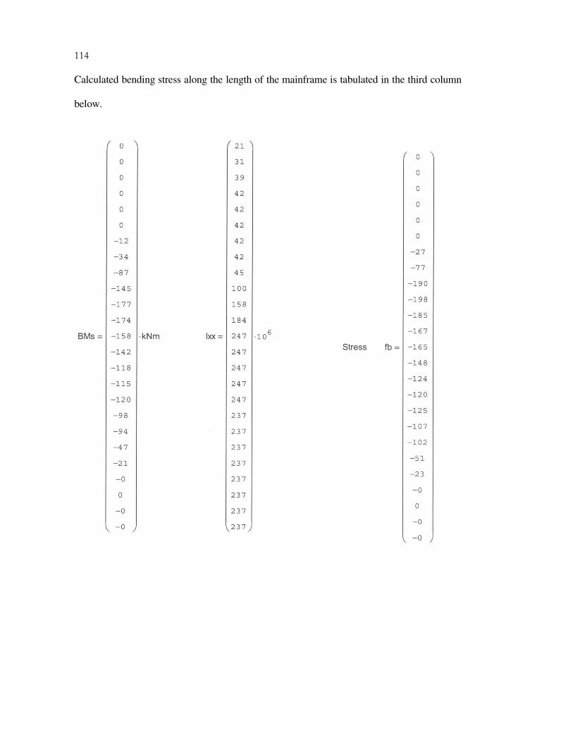
114

Calculated bending stress along the length of the mainframe is tabulated in the third column

below.