Embed Size (px)
Citation preview

Semi-Supervised Classificationlearning from labeled and unlabeled data
Xiaojin “Jerry” Zhu
Computer Science Department
University of Wisconsin, Madison
Semi-supervised classification. Xiaojin Zhu. Univ. Wisconsin-Madison – p. 1/76

“Eclipse”
Semi-supervised classification. Xiaojin Zhu. Univ. Wisconsin-Madison – p. 2/76
“Eclipse”
A good classifier needs good labeled training data.
Semi-supervised classification. Xiaojin Zhu. Univ. Wisconsin-Madison – p. 3/76

Labels can be hard to get
Human annotation is slow, boring
Semi-supervised classification. Xiaojin Zhu. Univ. Wisconsin-Madison – p. 4/76

Labels can be hard to get
Human annotation is slow, boring
It may require expert knowledge
Semi-supervised classification. Xiaojin Zhu. Univ. Wisconsin-Madison – p. 4/76
Labels can be hard to get
Human annotation is slow, boring
It may require expert knowledge
It may require special, expensive devices
Semi-supervised classification. Xiaojin Zhu. Univ. Wisconsin-Madison – p. 4/76
Labels can be hard to get
Human annotation is slow, boring
It may require expert knowledge
It may require special, expensive devices
Your graduate student is on vacation
Semi-supervised classification. Xiaojin Zhu. Univ. Wisconsin-Madison – p. 4/76
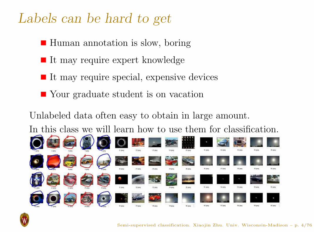
Labels can be hard to get
Human annotation is slow, boring
It may require expert knowledge
It may require special, expensive devices
Your graduate student is on vacation
Unlabeled data often easy to obtain in large amount.
In this class we will learn how to use them for classification.
Semi-supervised classification. Xiaojin Zhu. Univ. Wisconsin-Madison – p. 4/76
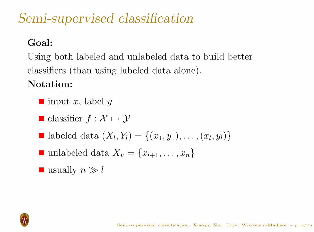
Semi-supervised classification
Goal:
Using both labeled and unlabeled data to build better
classifiers (than using labeled data alone).
Notation:
input x, label y
classifier f : X 7→ Y
labeled data (Xl, Yl) = {(x1, y1), . . . , (xl, yl)}
unlabeled data Xu = {xl+1, . . . , xn}
usually n ≫ l
Semi-supervised classification. Xiaojin Zhu. Univ. Wisconsin-Madison – p. 5/76

Outline
We will discuss some representative semi-supervised learning
methods
1. Self-training and Co-training
2. Generative probabilistic models
3. Semi-supervised support vector machines
4. Graph-based semi-supervised learning
Semi-supervised classification. Xiaojin Zhu. Univ. Wisconsin-Madison – p. 6/76

1. Self- and Co- Training
Semi-supervised classification. Xiaojin Zhu. Univ. Wisconsin-Madison – p. 7/76
Self-training
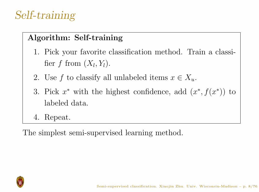
Algorithm: Self-training
1. Pick your favorite classification method. Train a classi-
fier f from (Xl, Yl).
2. Use f to classify all unlabeled items x ∈ Xu.
3. Pick x∗ with the highest confidence, add (x∗, f(x∗)) to
labeled data.
4. Repeat.
The simplest semi-supervised learning method.
Semi-supervised classification. Xiaojin Zhu. Univ. Wisconsin-Madison – p. 8/76

An example
Each image is divided into small patches
(10 × 10 grid, random size in 10 ∼ 20)
20 40 60 80 100 120 140
20
40
60
80
100
120
140
Semi-supervised classification. Xiaojin Zhu. Univ. Wisconsin-Madison – p. 9/76

An example
All patches are normalized.
Define a dictionary of 200 ‘visual words’ (cluster centroids)
with k-means clustering on all patches.
Patches represented by the index of the closest visual word.
Semi-supervised classification. Xiaojin Zhu. Univ. Wisconsin-Madison – p. 10/76
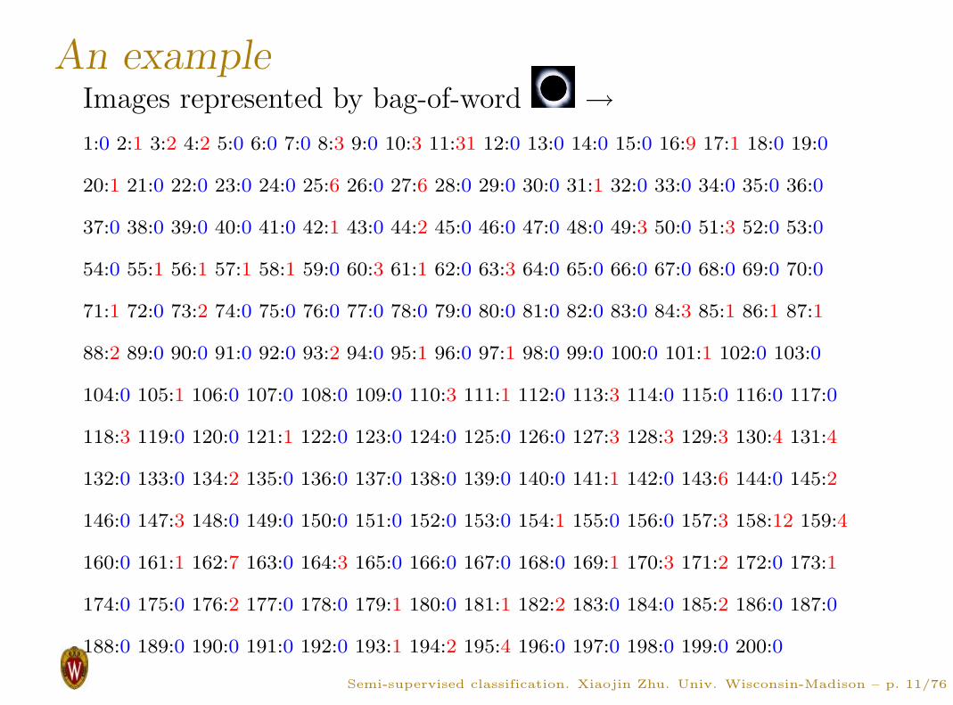
An exampleImages represented by bag-of-word →
1:0 2:1 3:2 4:2 5:0 6:0 7:0 8:3 9:0 10:3 11:31 12:0 13:0 14:0 15:0 16:9 17:1 18:0 19:0
20:1 21:0 22:0 23:0 24:0 25:6 26:0 27:6 28:0 29:0 30:0 31:1 32:0 33:0 34:0 35:0 36:0
37:0 38:0 39:0 40:0 41:0 42:1 43:0 44:2 45:0 46:0 47:0 48:0 49:3 50:0 51:3 52:0 53:0
54:0 55:1 56:1 57:1 58:1 59:0 60:3 61:1 62:0 63:3 64:0 65:0 66:0 67:0 68:0 69:0 70:0
71:1 72:0 73:2 74:0 75:0 76:0 77:0 78:0 79:0 80:0 81:0 82:0 83:0 84:3 85:1 86:1 87:1
88:2 89:0 90:0 91:0 92:0 93:2 94:0 95:1 96:0 97:1 98:0 99:0 100:0 101:1 102:0 103:0
104:0 105:1 106:0 107:0 108:0 109:0 110:3 111:1 112:0 113:3 114:0 115:0 116:0 117:0
118:3 119:0 120:0 121:1 122:0 123:0 124:0 125:0 126:0 127:3 128:3 129:3 130:4 131:4
132:0 133:0 134:2 135:0 136:0 137:0 138:0 139:0 140:0 141:1 142:0 143:6 144:0 145:2
146:0 147:3 148:0 149:0 150:0 151:0 152:0 153:0 154:1 155:0 156:0 157:3 158:12 159:4
160:0 161:1 162:7 163:0 164:3 165:0 166:0 167:0 168:0 169:1 170:3 171:2 172:0 173:1
174:0 175:0 176:2 177:0 178:0 179:1 180:0 181:1 182:2 183:0 184:0 185:2 186:0 187:0
188:0 189:0 190:0 191:0 192:0 193:1 194:2 195:4 196:0 197:0 198:0 199:0 200:0
Semi-supervised classification. Xiaojin Zhu. Univ. Wisconsin-Madison – p. 11/76

An example
1. Train a naıve Bayes classifier on initial labeled data
2. Classify unlabeled data, sort by confidence log p(y = a|x)
. . .
Semi-supervised classification. Xiaojin Zhu. Univ. Wisconsin-Madison – p. 12/76

An example
3. Add the most confident images (and computed labels) to
labeled data
4. Re-train classifier, classify unlabeled data, repeat
. . .
Semi-supervised classification. Xiaojin Zhu. Univ. Wisconsin-Madison – p. 13/76
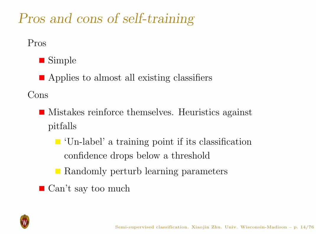
Pros and cons of self-training
Pros
Simple
Applies to almost all existing classifiers
Cons
Mistakes reinforce themselves. Heuristics against
pitfalls
‘Un-label’ a training point if its classification
confidence drops below a threshold
Randomly perturb learning parameters
Can’t say too much
Semi-supervised classification. Xiaojin Zhu. Univ. Wisconsin-Madison – p. 14/76

Co-training
Two views of an item: image and HTML text
Semi-supervised classification. Xiaojin Zhu. Univ. Wisconsin-Madison – p. 15/76

Feature split
Each item is represented by two kinds of features
x = [x(1); x(2)]
x(1) = image features
x(2) = web page text
This is a natural feature split (or multiple views)
Co-training idea:
Train an image classifier and a text classifier
The two classifiers teach each other
Semi-supervised classification. Xiaojin Zhu. Univ. Wisconsin-Madison – p. 16/76

Co-training algorithm
Algorithm: Co-training
1. Train two classifiers: f (1) from (X(1)l , Yl), f (2) from
(X(2)l , Yl).
2. Classify Xu with f (1) and f (2) separately.
3. Add f (1)’s k-most-confident (x, f (1)(x)) to f (2)’s labeled
data.
4. Add f (2)’s k-most-confident (x, f (2)(x)) to f (1)’s labeled
data.
5. Repeat.
Semi-supervised classification. Xiaojin Zhu. Univ. Wisconsin-Madison – p. 17/76

Co-training assumptions
Co-training assumes that
feature split x = [x(1); x(2)] exists
x(1) or x(2) alone is sufficient to train a good classifier
x(1) and x(2) are conditionally independent given the
class
X1 view X2 view
++
++
++
+
++
+
−
− −−
−
−−
−+
−++
++
++
+++
+++
+
+
++
− −
− −
−
−
−−
−
−−
−
+
+
+
++
+
+
+
++
+
−
−−
−−
−
−−
−
+++
+
+
+
+ +
+
+
+
+
+
++
+
−
−
−
−−
−−
−
−
−
−
−
Semi-supervised classification. Xiaojin Zhu. Univ. Wisconsin-Madison – p. 18/76

Pros and cons of co-training
Pros
Simple. Applies to almost all existing classifiers
Less sensitive to mistakes
Cons
Feature split may not exist
Models using BOTH features should do better
Semi-supervised classification. Xiaojin Zhu. Univ. Wisconsin-Madison – p. 19/76
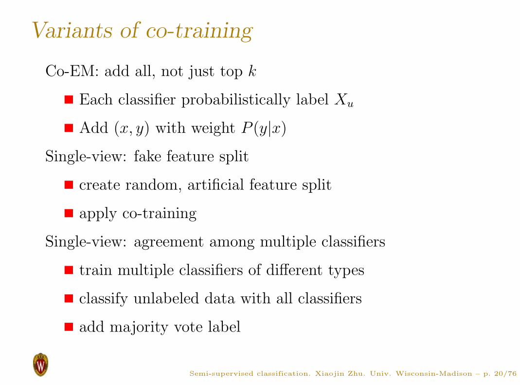
Variants of co-training
Co-EM: add all, not just top k
Each classifier probabilistically label Xu
Add (x, y) with weight P (y|x)
Single-view: fake feature split
create random, artificial feature split
apply co-training
Single-view: agreement among multiple classifiers
train multiple classifiers of different types
classify unlabeled data with all classifiers
add majority vote label
Semi-supervised classification. Xiaojin Zhu. Univ. Wisconsin-Madison – p. 20/76

2. Generative probabilisticmodels
Semi-supervised classification. Xiaojin Zhu. Univ. Wisconsin-Madison – p. 21/76

A simple example
Labeled data (Xl, Yl)
−5 −4 −3 −2 −1 0 1 2 3 4 5−5
−4
−3
−2
−1
0
1
2
3
4
5
Assuming each class has a Gaussian distribution in feature
space, what is the most likely decision boundary?
Semi-supervised classification. Xiaojin Zhu. Univ. Wisconsin-Madison – p. 22/76

The most-likely model
−5 −4 −3 −2 −1 0 1 2 3 4 5−5
−4
−3
−2
−1
0
1
2
3
4
5
Semi-supervised classification. Xiaojin Zhu. Univ. Wisconsin-Madison – p. 23/76
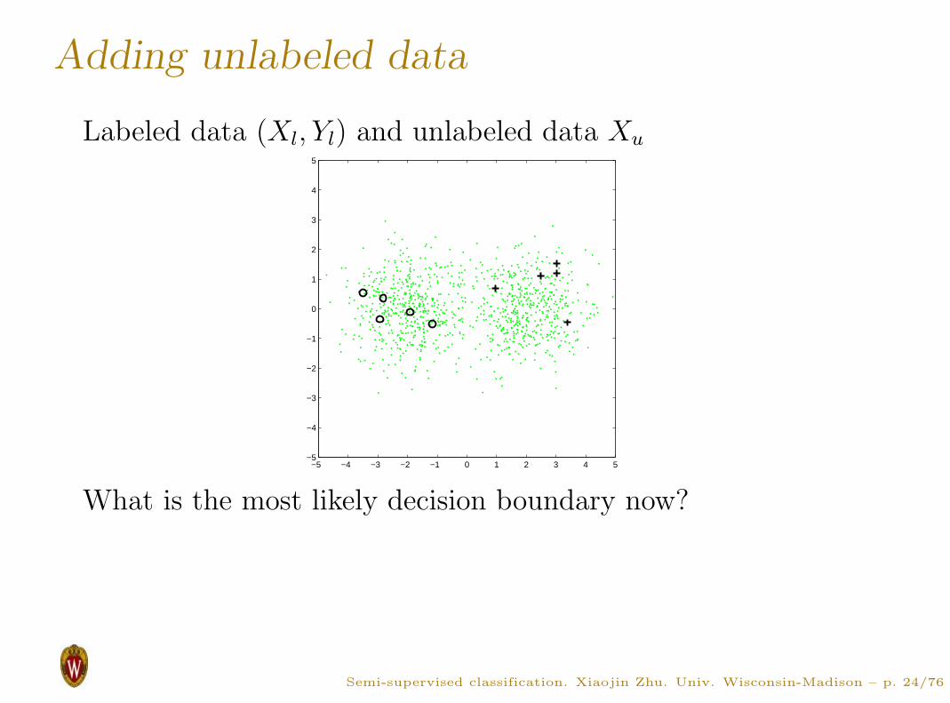
Adding unlabeled data
Labeled data (Xl, Yl) and unlabeled data Xu
−5 −4 −3 −2 −1 0 1 2 3 4 5−5
−4
−3
−2
−1
0
1
2
3
4
5
What is the most likely decision boundary now?
Semi-supervised classification. Xiaojin Zhu. Univ. Wisconsin-Madison – p. 24/76
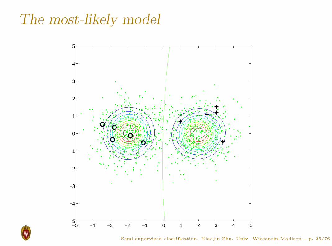
The most-likely model
−5 −4 −3 −2 −1 0 1 2 3 4 5−5
−4
−3
−2
−1
0
1
2
3
4
5
Semi-supervised classification. Xiaojin Zhu. Univ. Wisconsin-Madison – p. 25/76
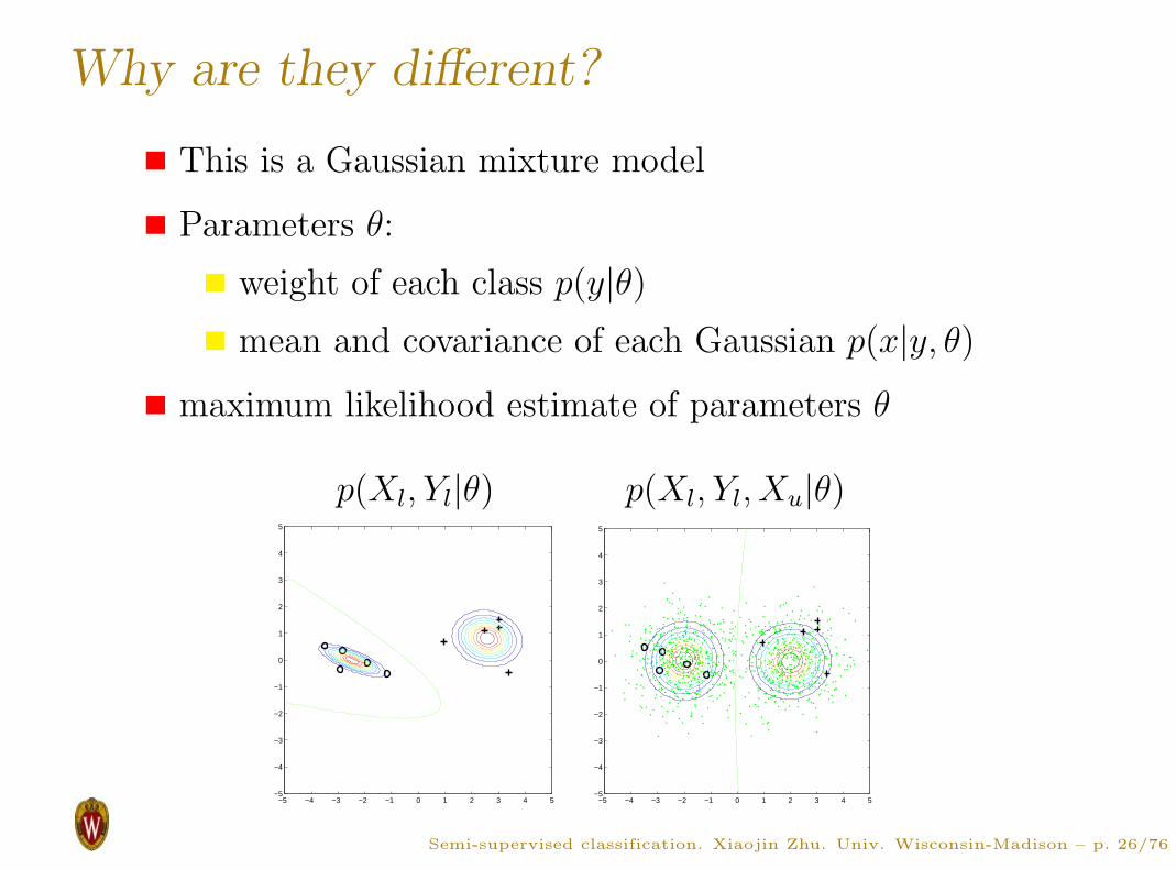
Why are they different?
This is a Gaussian mixture model
Parameters θ:
weight of each class p(y|θ)
mean and covariance of each Gaussian p(x|y, θ)
maximum likelihood estimate of parameters θ
p(Xl, Yl|θ) p(Xl, Yl, Xu|θ)
−5 −4 −3 −2 −1 0 1 2 3 4 5−5
−4
−3
−2
−1
0
1
2
3
4
5
−5 −4 −3 −2 −1 0 1 2 3 4 5−5
−4
−3
−2
−1
0
1
2
3
4
5
Semi-supervised classification. Xiaojin Zhu. Univ. Wisconsin-Madison – p. 26/76

Maximizing different likelihood
With labeled data only
log p(Xl, Yl|θ) =∑l
i=1 log p(yi|θ)p(xi|yi, θ)
maximum likelihood estimate (MLE) for θ trivial
With labeled and unlabeled data
log p(Xl, Yl, Xu|θ) =∑l
i=1 log p(yi|θ)p(xi|yi, θ)
+∑l+u
i=l+1 log(
∑2y=1 p(y|θ)p(xi|y, θ)
)
MLE harder (hidden variables)
Expectation-Maximization (EM), variational
approximation, etc.
Maximum a posteriori (MAP) possible with prior p(θ)
Semi-supervised classification. Xiaojin Zhu. Univ. Wisconsin-Madison – p. 27/76

Generative probabilistic models
A joint probabilistic model p(x, y|θ), e.g.,
Gaussian mixture models
Multinomial mixture models (Naive Bayes)
Latent Dirichlet allocation variants
Hidden Markov models (HMMs)
In contrast to discriminative models which model p(y|x)
directly (logistic regression, support vector machines,
conditional random fields etc.)
Semi-supervised classification. Xiaojin Zhu. Univ. Wisconsin-Madison – p. 28/76

Generative models algorithm
Algorithm: Generative models
1. Choose a generative model p(x, y|θ)
2. Find the MLE on labeled and unlabeled data
θ∗ = arg maxθ
p(Xl, Yl, Xu|θ)
3. Compute class distribution using Bayes’ rule
p(y|x, θ∗) =p(x, y|θ∗)
∑
y′ p(x, y′|θ∗)
We will discuss one method for finding θ∗: the EM
algorithm.
Semi-supervised classification. Xiaojin Zhu. Univ. Wisconsin-Madison – p. 29/76
EM for Gaussian mixture models
Start from MLE θ on (Xl, Yl)
p(y|θ): proportion of data with label y
p(x|y, θ): mean and covariance of data with label y
Repeat the two steps
1. E-step: compute the expected labels p(y|x, θ) for all
x ∈ Xu
assign class 1 to p(y = 1|x, θ) fraction of x
assign class 2 to p(y = 2|x, θ) fraction of x
2. M-step: update MLE θ with the original labeled and
(now labeled) unlabeled data
Semi-supervised classification. Xiaojin Zhu. Univ. Wisconsin-Madison – p. 30/76
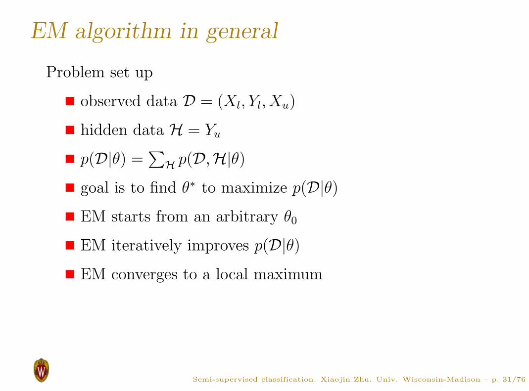
EM algorithm in general
Problem set up
observed data D = (Xl, Yl, Xu)
hidden data H = Yu
p(D|θ) =∑
Hp(D,H|θ)
goal is to find θ∗ to maximize p(D|θ)
EM starts from an arbitrary θ0
EM iteratively improves p(D|θ)
EM converges to a local maximum
Semi-supervised classification. Xiaojin Zhu. Univ. Wisconsin-Madison – p. 31/76

How EM works
Instead of p(D|θ), EM works on log p(D|θ) ≡ L(θ)
EM constructs a lower bound F(q, θ) ≤ L(θ)
auxiliary distribution q
Jensen’s inequality, concavity of log
F(q, θ) is easier to optimize than L(θ)
coordinate ascent
fix θ, optimize q: the E-step
fix q, optimize θ: the M-step
Semi-supervised classification. Xiaojin Zhu. Univ. Wisconsin-Madison – p. 32/76

Jensen’s inequality on log()
∀∑
qi = 1, qi ≥ 0, log∑
qihi ≥∑
qi log hi
0 0.5 1 1.5 2−2.5
−2
−1.5
−1
−0.5
0
0.5
1
log(h1)
log(h2)
0.5 log(h1) + 0.5 log(h
2)
log(0.5 h1 + 0.5 h
2)
Semi-supervised classification. Xiaojin Zhu. Univ. Wisconsin-Madison – p. 33/76
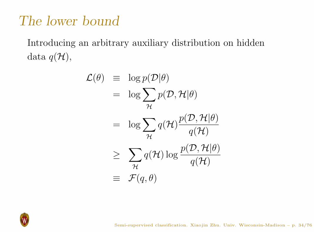
The lower bound
Introducing an arbitrary auxiliary distribution on hidden
data q(H),
L(θ) ≡ log p(D|θ)
= log∑
H
p(D,H|θ)
= log∑
H
q(H)p(D,H|θ)
q(H)
≥∑
H
q(H) logp(D,H|θ)
q(H)
≡ F(q, θ)
Semi-supervised classification. Xiaojin Zhu. Univ. Wisconsin-Madison – p. 34/76

Coordinate ascent on q
Fixing θ, F(q, θ) is maximizes when
∂
∂q(H)q(H) log
p(D,H|θ)
q(H)= 0
s.t.∑
H
q(H) = 1
The maximizing q∗(H) = p(H|D, θ)
q∗(H) is the expected label under θ
The E-step
Under q∗(H), F(q∗, θ) = L(θ): the lower bound is tight
Semi-supervised classification. Xiaojin Zhu. Univ. Wisconsin-Madison – p. 35/76

Coordinate ascent on θ
Fixing q∗, F(q∗, θ) is maximized by maximizing
∑
H
q∗(H) log p(D,H|θ)
‘Fractional’ labels with probability q∗(H)
The M-step
EM never decreases likelihood:
L(θ)E-step
= F(q∗, θ)M-step
≤ F(q∗, θ′)Jensen
≤ L(θ′)
EM converges to a local maximum.
Semi-supervised classification. Xiaojin Zhu. Univ. Wisconsin-Madison – p. 36/76

Review: Generative models algorithm
Algorithm: Generative models
1. Choose a generative model p(x, y|θ)
2. Find the MLE on labeled and unlabeled data
θ∗ = arg maxθ
p(Xl, Yl, Xu|θ)
EM is one method.
3. Compute class distribution using Bayes’ rule
p(y|x, θ∗) =p(x, y|θ∗)
∑
y′ p(x, y′|θ∗)
The Baum-Welch algorithm for HMMs is a form of EM, or
semi-supervised learning method.
Semi-supervised classification. Xiaojin Zhu. Univ. Wisconsin-Madison – p. 37/76

Pros and cons of generative models
Pro: clear probabilistic framework
Con: unlabeled data may hurt if generative model is
wrong
−6 −4 −2 0 2 4 6−6
−4
−2
0
2
4
6
Class 1
Class 2
Semi-supervised classification. Xiaojin Zhu. Univ. Wisconsin-Madison – p. 38/76
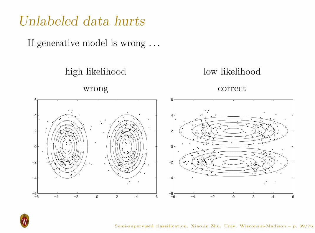
Unlabeled data hurts
If generative model is wrong . . .
high likelihood low likelihood
wrong correct
−6 −4 −2 0 2 4 6−6
−4
−2
0
2
4
6
−6 −4 −2 0 2 4 6−6
−4
−2
0
2
4
6
Semi-supervised classification. Xiaojin Zhu. Univ. Wisconsin-Madison – p. 39/76

Briefly mentioned
Clustering algorithms can be used for semi-supervised
classification too:
Run your favorite clustering algorithm on Xl, Xu.
Label all points within a cluster by the majority of
labeled points in the cluster.
Pro: Yet another simple method using existing algorithms.
Con: Hard to analyze.
Semi-supervised classification. Xiaojin Zhu. Univ. Wisconsin-Madison – p. 40/76

3. Semi-SupervisedSupport Vector Machines
Semi-supervised classification. Xiaojin Zhu. Univ. Wisconsin-Madison – p. 41/76
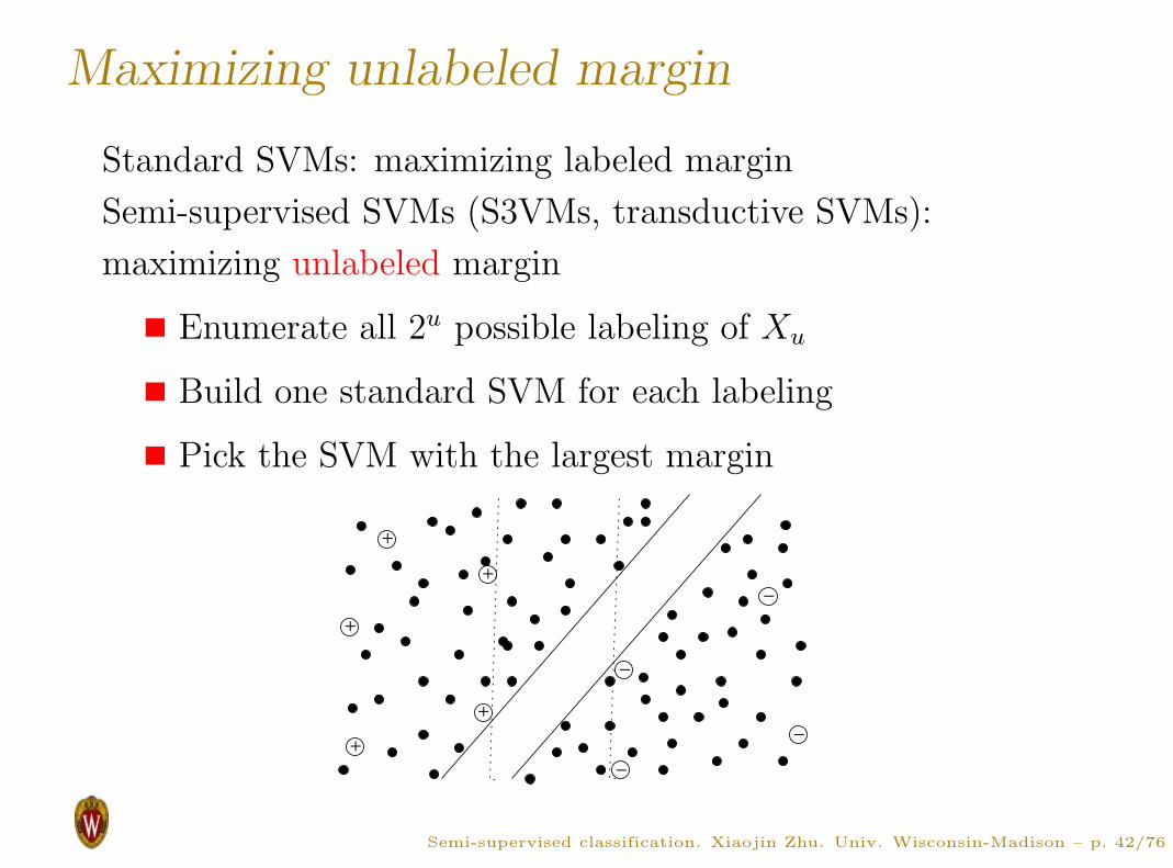
Maximizing unlabeled margin
Standard SVMs: maximizing labeled margin
Semi-supervised SVMs (S3VMs, transductive SVMs):
maximizing unlabeled margin
Enumerate all 2u possible labeling of Xu
Build one standard SVM for each labeling
Pick the SVM with the largest margin
+
+
+
+
+
−
−
−
−
Semi-supervised classification. Xiaojin Zhu. Univ. Wisconsin-Madison – p. 42/76

SVM review
The setting of support vector machines
two classes y ∈ {+1,−1}
labeled data (Xl, Yl)
a kernel K
the reproducing Hilbert kernel space HK
SVM finds a function f(x) = h(x) + b with h ∈ HK
Classify x by sign(f(x))
Semi-supervised classification. Xiaojin Zhu. Univ. Wisconsin-Madison – p. 43/76

Linearly separable SVMs
The linearly separable SVM: all training points must be
outside the corresponding margin.
minh,b
‖h‖2HK
subject to h(xi) + b ≥ 1 , if yi = 1 ∀i = 1 . . . l
h(xi) + b ≤ −1 , if yi = −1
The two constraints can be written as
yi(h(xi) + b) ≥ 1 ∀i = 1 . . . l
Data may not be linearly separable, even in HK .
Semi-supervised classification. Xiaojin Zhu. Univ. Wisconsin-Madison – p. 44/76
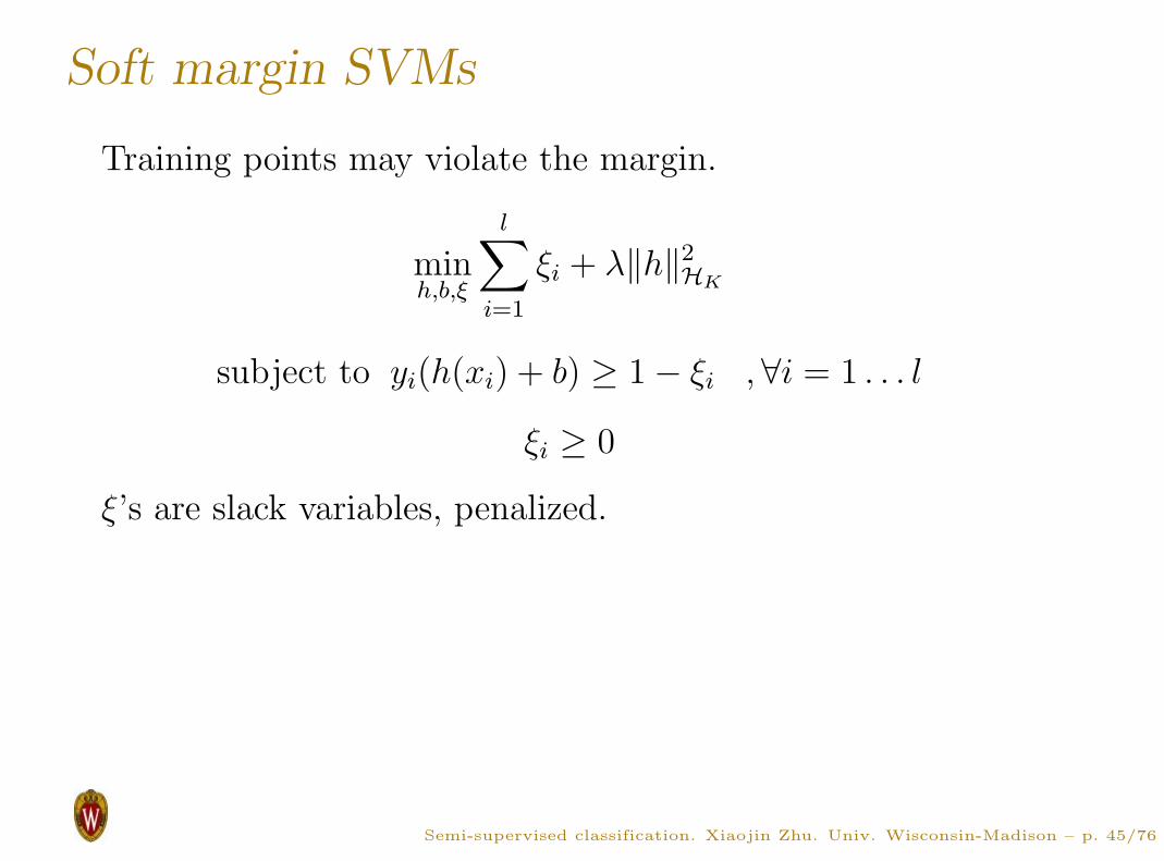
Soft margin SVMs
Training points may violate the margin.
minh,b,ξ
l∑
i=1
ξi + λ‖h‖2HK
subject to yi(h(xi) + b) ≥ 1 − ξi ,∀i = 1 . . . l
ξi ≥ 0
ξ’s are slack variables, penalized.
Semi-supervised classification. Xiaojin Zhu. Univ. Wisconsin-Madison – p. 45/76

Hinge function
minξ
ξ
subject to ξ ≥ z
ξ ≥ 0
If z ≤ 0, min ξ = 0
If z > 0, min ξ = z
Therefore the constrained optimization problem above is
equivalent to the hinge function
(z)+ = max(z, 0)
Semi-supervised classification. Xiaojin Zhu. Univ. Wisconsin-Madison – p. 46/76

SVM with hinge function
Let zi = 1 − yi(h(xi) + b) = 1 − yif(xi), the problem
minh,b,ξ
l∑
i=1
ξi + λ‖h‖2HK
subject to yi(h(xi) + b) ≥ 1 − ξi ,∀i = 1 . . . l
ξi ≥ 0
is equivalent to
minf
l∑
i=1
(1 − yif(xi))+ + λ‖h‖2HK
Semi-supervised classification. Xiaojin Zhu. Univ. Wisconsin-Madison – p. 47/76
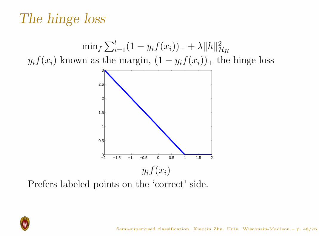
The hinge loss
minf
∑l
i=1(1 − yif(xi))+ + λ‖h‖2HK
yif(xi) known as the margin, (1 − yif(xi))+ the hinge loss
−2 −1.5 −1 −0.5 0 0.5 1 1.5 20
0.5
1
1.5
2
2.5
3
yif(xi)
Prefers labeled points on the ‘correct’ side.
Semi-supervised classification. Xiaojin Zhu. Univ. Wisconsin-Madison – p. 48/76
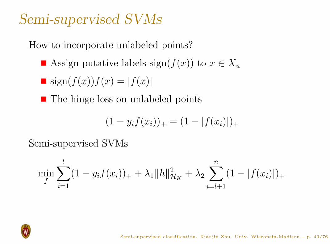
Semi-supervised SVMs
How to incorporate unlabeled points?
Assign putative labels sign(f(x)) to x ∈ Xu
sign(f(x))f(x) = |f(x)|
The hinge loss on unlabeled points
(1 − yif(xi))+ = (1 − |f(xi)|)+
Semi-supervised SVMs
minf
l∑
i=1
(1 − yif(xi))+ + λ1‖h‖2HK
+ λ2
n∑
i=l+1
(1 − |f(xi)|)+
Semi-supervised classification. Xiaojin Zhu. Univ. Wisconsin-Madison – p. 49/76
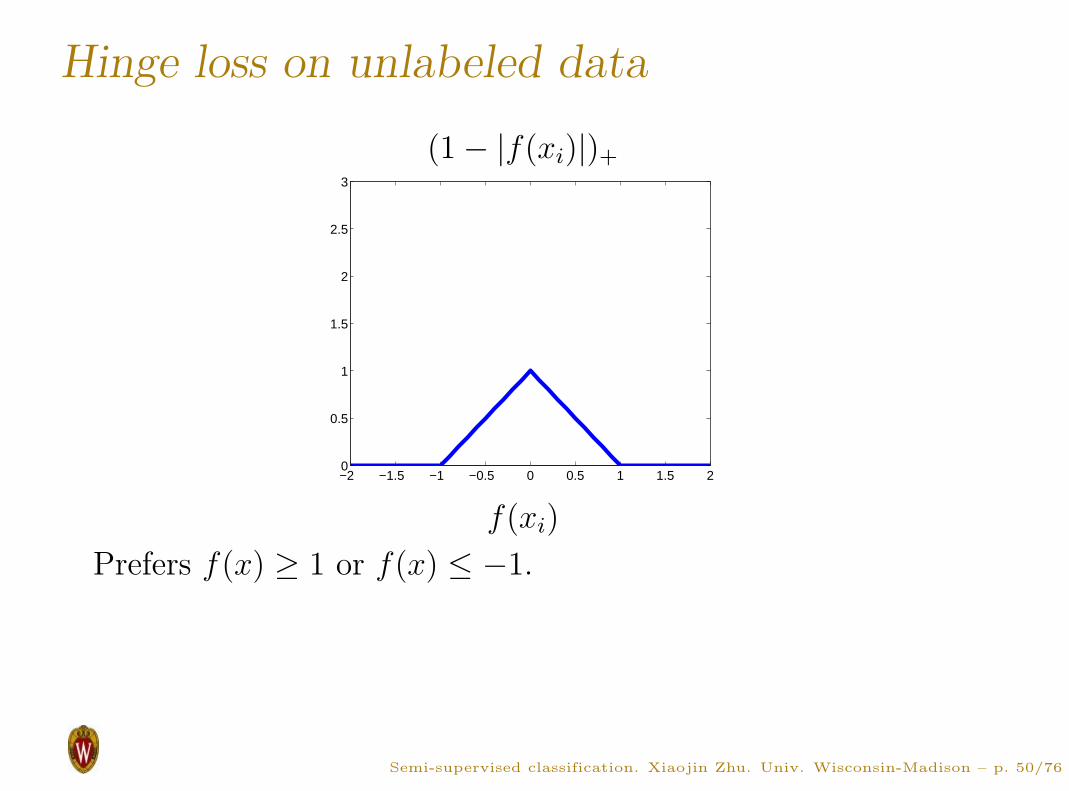
Hinge loss on unlabeled data
(1 − |f(xi)|)+
−2 −1.5 −1 −0.5 0 0.5 1 1.5 20
0.5
1
1.5
2
2.5
3
f(xi)
Prefers f(x) ≥ 1 or f(x) ≤ −1.
Semi-supervised classification. Xiaojin Zhu. Univ. Wisconsin-Madison – p. 50/76
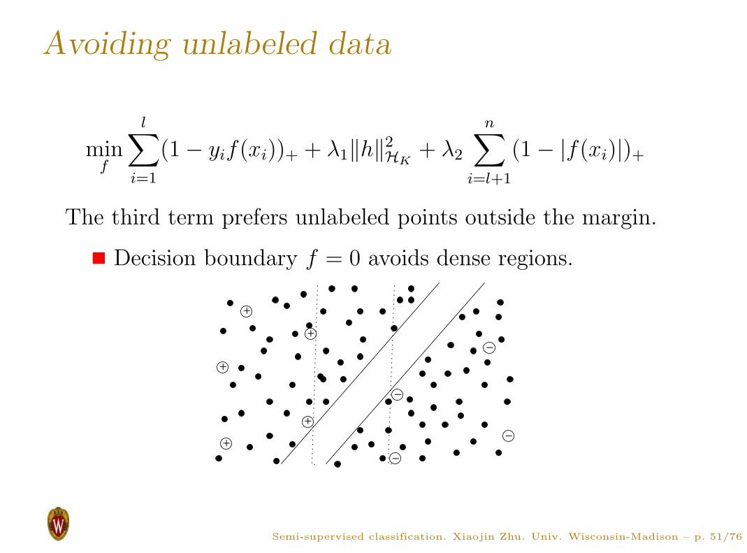
Avoiding unlabeled data
minf
l∑
i=1
(1 − yif(xi))+ + λ1‖h‖2HK
+ λ2
n∑
i=l+1
(1 − |f(xi)|)+
The third term prefers unlabeled points outside the margin.
Decision boundary f = 0 avoids dense regions.
+
+
+
+
+
−
−
−
−
Semi-supervised classification. Xiaojin Zhu. Univ. Wisconsin-Madison – p. 51/76
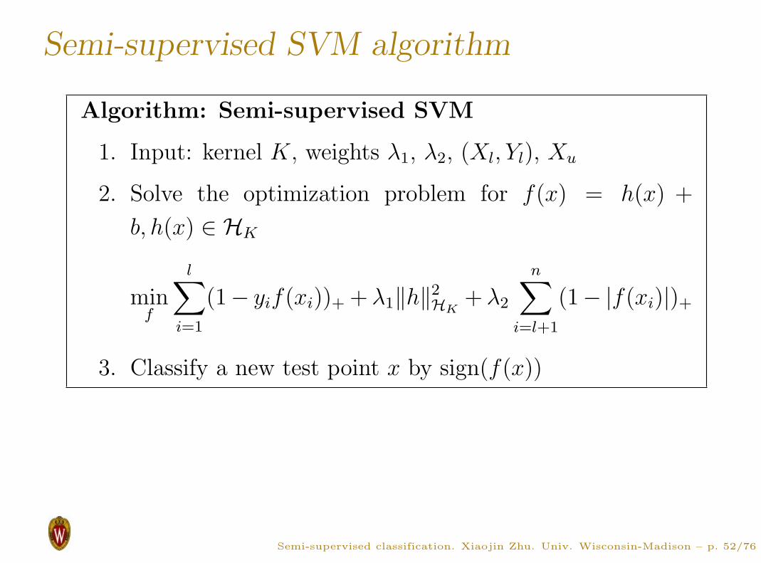
Semi-supervised SVM algorithm
Algorithm: Semi-supervised SVM
1. Input: kernel K, weights λ1, λ2, (Xl, Yl), Xu
2. Solve the optimization problem for f(x) = h(x) +
b, h(x) ∈ HK
minf
l∑
i=1
(1− yif(xi))+ + λ1‖h‖2HK
+ λ2
n∑
i=l+1
(1− |f(xi)|)+
3. Classify a new test point x by sign(f(x))
Semi-supervised classification. Xiaojin Zhu. Univ. Wisconsin-Madison – p. 52/76
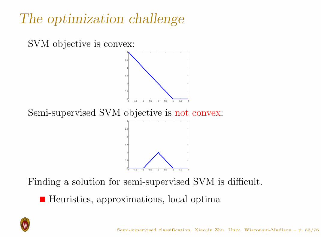
The optimization challenge
SVM objective is convex:
−2 −1.5 −1 −0.5 0 0.5 1 1.5 20
0.5
1
1.5
2
2.5
3
Semi-supervised SVM objective is not convex:
−2 −1.5 −1 −0.5 0 0.5 1 1.5 20
0.5
1
1.5
2
2.5
3
Finding a solution for semi-supervised SVM is difficult.
Heuristics, approximations, local optima
Semi-supervised classification. Xiaojin Zhu. Univ. Wisconsin-Madison – p. 53/76

Pros and Cons of S3VMs
Pros:
Applicable wherever SVMs are applicable
Clear mathematical framework
Cons:
Avoiding unlabeled dense region may not be the right
assumption
Optimization difficult, (currently) slow
Semi-supervised classification. Xiaojin Zhu. Univ. Wisconsin-Madison – p. 54/76
4. Graph-BasedSemi-Supervised Learning
Semi-supervised classification. Xiaojin Zhu. Univ. Wisconsin-Madison – p. 55/76
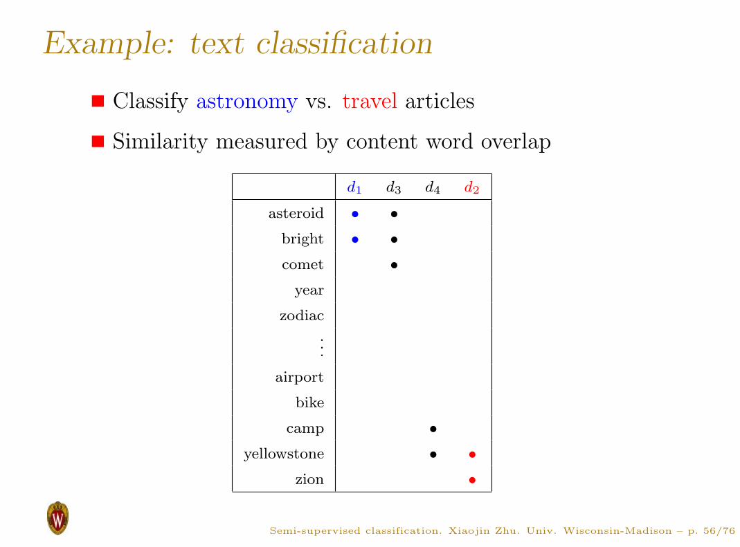
Example: text classification
Classify astronomy vs. travel articles
Similarity measured by content word overlap
d1 d3 d4 d2
asteroid • •
bright • •
comet •
year
zodiac
.
..
airport
bike
camp •
yellowstone • •
zion •
Semi-supervised classification. Xiaojin Zhu. Univ. Wisconsin-Madison – p. 56/76
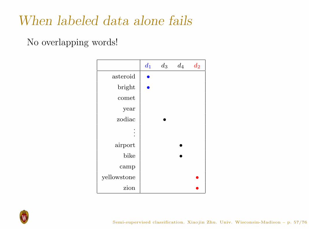
When labeled data alone fails
No overlapping words!
d1 d3 d4 d2
asteroid •
bright •
comet
year
zodiac •
...
airport •
bike •
camp
yellowstone •
zion •
Semi-supervised classification. Xiaojin Zhu. Univ. Wisconsin-Madison – p. 57/76

Unlabeled data: stepping stones
Labels propagate via similar unlabeled articles.
d1 d5 d6 d7 d3 d4 d8 d9 d2
asteroid •
bright • •
comet • •
year • •
zodiac • •
...
airport •
bike • •
camp • •
yellowstone • •
zion •
Semi-supervised classification. Xiaojin Zhu. Univ. Wisconsin-Madison – p. 58/76

Another example
Handwritten digits recognition with pixel-wise Euclidean
distance
not similar ‘indirectly’ similar
with stepping stones
Semi-supervised classification. Xiaojin Zhu. Univ. Wisconsin-Madison – p. 59/76

The graph
Nodes: Xl ∪ Xu
Edges: similarity weights computed from features, e.g.,
k-nearest-neighbor graph, unweighted (0, 1 weights)
fully connected graph, weight decays with distance
w = exp (−‖xi − xj‖2/σ2)
Want: implied similarity via all paths
d1
d2
d4
d3
Semi-supervised classification. Xiaojin Zhu. Univ. Wisconsin-Madison – p. 60/76
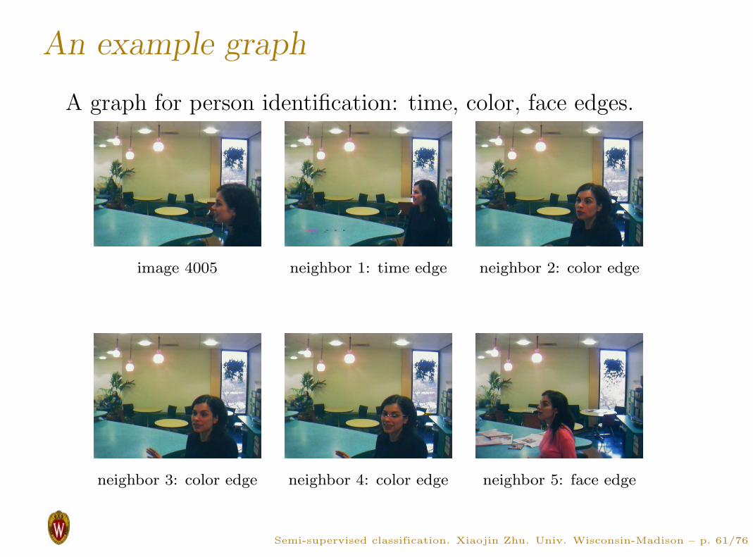
An example graph
A graph for person identification: time, color, face edges.
image 4005 neighbor 1: time edge neighbor 2: color edge
neighbor 3: color edge neighbor 4: color edge neighbor 5: face edge
Semi-supervised classification. Xiaojin Zhu. Univ. Wisconsin-Madison – p. 61/76
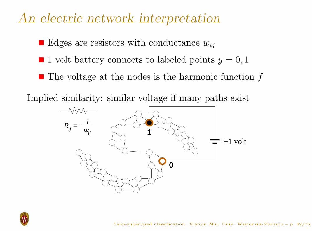
An electric network interpretation
Edges are resistors with conductance wij
1 volt battery connects to labeled points y = 0, 1
The voltage at the nodes is the harmonic function f
Implied similarity: similar voltage if many paths exist
+1 volt
wijR =ij
1
1
0
Semi-supervised classification. Xiaojin Zhu. Univ. Wisconsin-Madison – p. 62/76
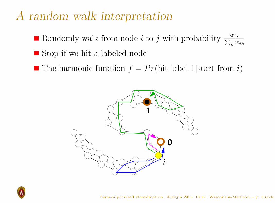
A random walk interpretation
Randomly walk from node i to j with probabilitywij
P
k wik
Stop if we hit a labeled node
The harmonic function f = Pr(hit label 1|start from i)
Semi-supervised classification. Xiaojin Zhu. Univ. Wisconsin-Madison – p. 63/76

The harmonic function
The harmonic function f satisfies
f(xi) = yi for i = 1 . . . l
f minimizes the energy∑
i∼j
wij(f(xi) − f(xj))2
average of neighbors f(xi) =P
j∼i wijf(xj)P
j∼i wij,∀xi ∈ Xu
We compute f using the graph Laplacian.
Semi-supervised classification. Xiaojin Zhu. Univ. Wisconsin-Madison – p. 64/76
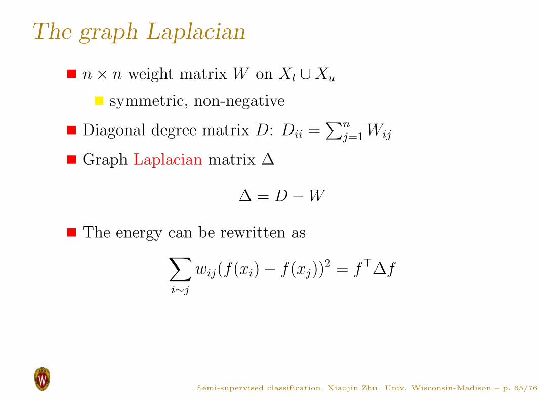
The graph Laplacian
n × n weight matrix W on Xl ∪ Xu
symmetric, non-negative
Diagonal degree matrix D: Dii =∑n
j=1 Wij
Graph Laplacian matrix ∆
∆ = D − W
The energy can be rewritten as∑
i∼j
wij(f(xi) − f(xj))2 = f⊤∆f
Semi-supervised classification. Xiaojin Zhu. Univ. Wisconsin-Madison – p. 65/76

Harmonic solution with Laplacian
The harmonic solution minimizes energy subject to the
given labels
minf
∞
l∑
i=1
(f(xi) − yi)2 + f⊤∆f
Partition the Laplacian matrix ∆ =
∆ll ∆lu
∆ul ∆uu
Harmonic solution
fu = −∆uu−1∆ulYl
Semi-supervised classification. Xiaojin Zhu. Univ. Wisconsin-Madison – p. 66/76

Graph spectrum ∆ =∑n
i=1 λiφiφ⊤i
λ1=0.00 λ
2=0.00 λ
3=0.04 λ
4=0.17 λ
5=0.38
λ6=0.38 λ
7=0.66 λ
8=1.00 λ
9=1.38 λ
10=1.38
λ11
=1.79 λ12
=2.21 λ13
=2.62 λ14
=2.62 λ15
=3.00
λ16
=3.34 λ17
=3.62 λ18
=3.62 λ19
=3.83 λ20
=3.96
Semi-supervised classification. Xiaojin Zhu. Univ. Wisconsin-Madison – p. 67/76
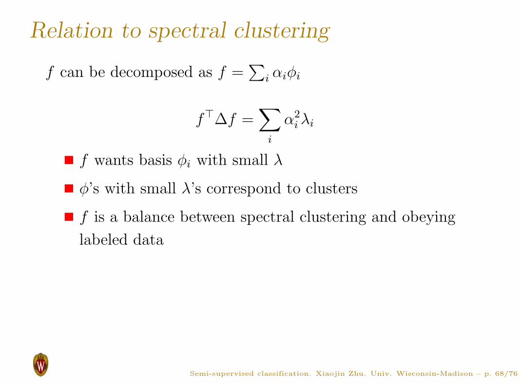
Relation to spectral clustering
f can be decomposed as f =∑
i αiφi
f⊤∆f =∑
i
α2i λi
f wants basis φi with small λ
φ’s with small λ’s correspond to clusters
f is a balance between spectral clustering and obeying
labeled data
Semi-supervised classification. Xiaojin Zhu. Univ. Wisconsin-Madison – p. 68/76
Problems with harmonic solution
Harmonic solution has two issues
It fixes the given labels Yl
What if some labels are wrong?
Want to be flexible and disagree with given labels
occasionally
It cannot handle new test points directly
f is only defined on Xu
We have to add new test points to the graph, and
find a new harmonic solution
Semi-supervised classification. Xiaojin Zhu. Univ. Wisconsin-Madison – p. 69/76

Manifold regularization
Manifold regularization solves the two issues
Allows but penalizes f(Xl) 6= Yi using hinge loss
Automatically applies to new test data
Defines function in kernel K induced RKHS:
f(x) = h(x) + b, h(x) ∈ HK
Still prefers low energy f⊤1:n∆f1:n
minf
l∑
i=1
(1 − yif(xi))+ + λ1‖h‖2HK
+ λ2f⊤
1:n∆f1:n
Semi-supervised classification. Xiaojin Zhu. Univ. Wisconsin-Madison – p. 70/76

Manifold regularization algorithm
Algorithm: Manifold regularization algorithm
1. Input: kernel K, weights λ1, λ2, (Xl, Yl), Xu
2. Construct similarity graph W from Xl, Xu, compute
graph Laplacian ∆
3. Solve the optimization problem for f(x) = h(x) +
b, h(x) ∈ HK
minf
l∑
i=1
(1 − yif(xi))+ + λ1‖h‖2HK
+ λ2f⊤
1:n∆f1:n
4. Classify a new test point x by sign(f(x))
Semi-supervised classification. Xiaojin Zhu. Univ. Wisconsin-Madison – p. 71/76
Pros and Cons of graph-based method
Pros:
Clear mathematical framework
Performance is good if the graph is good
Cons:
Performance is bad if the graph is bad
How to construct a good graph?
Semi-supervised classification. Xiaojin Zhu. Univ. Wisconsin-Madison – p. 72/76

Summary
Semi-supervised classification. Xiaojin Zhu. Univ. Wisconsin-Madison – p. 73/76

Which method is the best?
They make different assumptions
co-training: feature split, conditional independence
generative model: the particular model
S3VM: avoid dense regions
graph-based: edge weights
On-going research.
Semi-supervised classification. Xiaojin Zhu. Univ. Wisconsin-Madison – p. 74/76
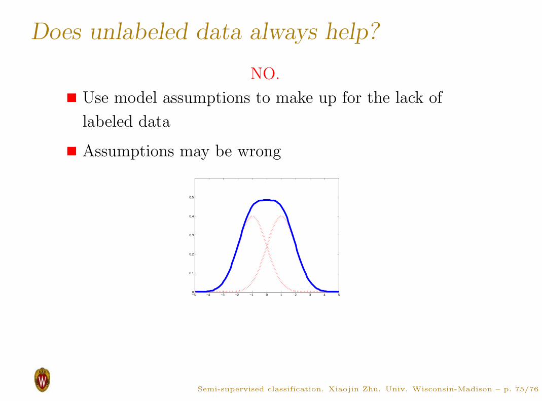
Does unlabeled data always help?
NO.
Use model assumptions to make up for the lack of
labeled data
Assumptions may be wrong
−5 −4 −3 −2 −1 0 1 2 3 4 50
0.1
0.2
0.3
0.4
0.5
Semi-supervised classification. Xiaojin Zhu. Univ. Wisconsin-Madison – p. 75/76

References
1. Xiaojin Zhu (2005). Semi-supervised learning literature
survey. TR-1530. University of Wisconsin-Madison
Department of Computer Science.
2. Olivier Chapelle, Alexander Zien, Bernhard Scholkopf
(Eds.). (2006). Semi-supervised learning. MIT Press.
3. Matthias Seeger (2001). Learning with labeled and
unlabeled data. Technical Report. University of
Edinburgh.
Semi-supervised classification. Xiaojin Zhu. Univ. Wisconsin-Madison – p. 76/76


![Semi-supervised Learning with Ladder Networkspapers.nips.cc/...semi-supervised-learning-with-ladder-networks.pdf · Semi-Supervised Learning with Ladder Networks ... 3] or classification](https://img.pdfslide.us/doc/110x75/5af9e4237f8b9ae92b8cfd03/semi-supervised-learning-with-ladder-learning-with-ladder-networks-3-or-classication.jpg)