Operations Research Letters 30 (2002) 408–414

OperationsResearchLetters

www.elsevier.com/locate/dsw

Semi-on-line problems on two identical machineswith combined partial information�

Zhiyi Tana;b, Yong Heb;∗

aCollege of Electronic Engineering, Zhejiang University, Hangzhou 310027, People’s Republic of ChinabDepartment of Mathematics, Zhejiang University, Hangzhou 310027, People’s Republic of China

Received 11 February 2002; received in revised form 16 April 2002; accepted 10 May 2002

Abstract

This paper considers the semi-on-line versions of scheduling problem P2‖Cmax. We study the semi-on-line problems withcombination of two types of information. Five basic types of partial information are considered. For two kinds of pairwisecombination, we present their respective optimal semi-on-line algorithms which show that combination can admit to constructbetter algorithms. c© 2002 Elsevier Science B.V. All rights reserved.

MSC: 90B35; 90C27

Keywords: Semi-on-line; Parallel machine scheduling; Approximation algorithm; Competitive analysis

1. Introduction

In most literature on scheduling theory, problemsare classi<ed as o=-line and on-line [2]. If full infor-mation on jobs to be scheduled is available in advance,we call the scheduling problem o+-line. By contrast,if the jobs are not known a priori, but arrive one byone, and we are required to schedule jobs irrevocablyon the machines as soon as they are given, withoutany knowledge about jobs that follow later on, thisproblem is called on-line.

With the development of scheduling theory and ap-plication, such classi<cation is not suBcient to in-clude all scheduling problems discussed. In recentyears, semi-on-line scheduling problems gained much

� This research is supported by TRAPOYT of China, NSFCof China (19701028) and National 973 Fundamental ResearchProject of China (1998030401(2)).

∗ Corresponding author.E-mail address: heyong@math.zju.edu.cn (Y. He).

interest due to their increased application in prac-tice [1,3,6,7]. Here, a scheduling problem is calledsemi-on-line if some partial additional informationabout jobs is available in advance, and we cannot re-arrange any job which has been assigned to machines.Semi-on-line is neither o=-line nor on-line, but some-how in between. Though it is a relatively new area,various papers and enormous results appeared in thelast decade [4,8,10,11].

For semi-on-line scheduling problems, we still usecompetitive analysis to measure the performance ofapproximation algorithms. Competitive analysis is atype of worst-case analysis where the performanceof an on-line or semi-on-line algorithm is comparedto that of an optimal o=-line algorithm [9]. For anon-line or semi-on-line algorithm A, let CA denote themakespan of a schedule produced by A, and COPT

denote the corresponding makespan of some optimalschedule. Then the competitive ratio of A is de<nedas the smallest number c such that CA6 cCOPT forall instances. An algorithm with a competitive ratio

0167-6377/02/$ - see front matter c© 2002 Elsevier Science B.V. All rights reserved.PII: S 0167 -6377(02)00164 -5

Z. Tan, Y. He / Operations Research Letters 30 (2002) 408–414 409

c is called c-competitive algorithm. An on-line orsemi-on-line problem has a lower bound � if no on-lineor semi-on-line algorithm can be �′-competitive with�′ ¡ �. An on-line or semi-on-line algorithm is calledoptimal if its competitive ratio matches the lowerbound of the on-line or semi-on-line problem.

In general, in a semi-on-line version of a problemthe conditions to be considered on-line are somehowrelaxed. Di=erent ways of relaxing the conditions giverise to di=erent semi-on-line versions; one wishes toachieve improvement of the performance of the opti-mal semi-on-line algorithm with respect to the on-lineversion by using additional information. Let us takethe most classical scheduling problem P2‖Cmax as anexample. It is clear that List Scheduling (LS) is anoptimal on-line algorithm with competitive ratio 3

2 . In[6], Kellerer et al., considered a semi-on-line versionwhere the total processing time of all jobs is knownin advance. They presented an optimal semi-on-linealgorithm H3 with competitive ratio 4

3 . In [5], He andZhang considered a semi-on-line version where thelargest processing time of all jobs is known in ad-vance. They presented an optimal semi-on-line algo-rithm PLS with competitive ratio 4

3 , too. In [8], Seidenet al., studied another semi-on-line version where jobsarrive in order of non-increasing processing times.They proved LS is still an optimal semi-on-line algo-rithm with competitive ratio 7

6 .To shed further light on the usefulness of di=er-

ent types of information, in this paper we considerwhether the combination of two types of informationcan admit to construct a semi-on-line algorithm withmuch smaller competitive ratio than that of the casewhere only one type of information is available in ad-vance. In fact, even the combination of two uselesstypes of information may reach a satisfactory result.For example, in [12], Zhang and Ye considered thecombination of information suggestive and LargestLast. The <rst type of information means that at thetime the last job arrives, the scheduler is informedthat it is indeed the last one. The second one meansthat the last job of the instance is the largest one.Each type of the above information itself is useless,which can be proved by job sequences with process-ing times {1; 1; 2} and {1; 1; �}; {1; 1} and {1; 1; 2},respectively, where � ¿ 0 and � → 0. But algorithmA1 presented in [12] is an optimal semi-on-line algo-rithm with competitive ratio

√2 for this problem.

This paper is organized as follows. In Section 2, wewill give some basic notations and preliminary results.In Sections 3 and 4, we will consider two semi-on-lineversions where two types of additional informationare combined, and present their respective optimal al-gorithms with smaller competitive ratios than thoseof the versions where only one information is avail-able in advance. Finally some conclusions are madein Section 5.

2. Preliminary

The scheduling problem P2‖Cmax can be describedas follows: We are given a set J = {p1; p2; : : : ; pn}of independent jobs, each with a positive process-ing time, that must be scheduled on two parallelidentical machines M1 and M2. We identify the jobswith their processing times. The machines are avail-able at time zero and no preemption is allowed.The objective is to minimize the overall completiontime Cmax, called makespan. Five basic semi-on-lineversions concerned in our paper are listed asfollows.

sum: The total processing time of all jobs T=∑n

j=1 pi

is known in advance.max: The largest processing time of all jobs pmax =

max16j6n pj is known in advance.decr: Jobs arrive in order of non-increasing processing

times, i.e. pi¿pi+1; i¿ 1.sugg: At the same time the last job arrives, we will be

indicating that this is the last one.LL: The last job pn has the largest processing time,

i.e. pn = pmax.

We use P2|s|Cmax to denote the semi-on-line prob-lem with information s, where s∈{sum; max; sugg;decr; LL}. Moreover, we use P2|s1 & s2|Cmax to de-note the semi-on-line problem where both informa-tion s1 and s2 are available in advance. The followinglemma is trivial but useful.

Lemma 2.1. (1) If the lower bounds of P2|s1|Cmax;P2|s2|Cmax and P2|s1 & s2|Cmax are c1; c2; and c12;respectively; then we have c126min {c1; c2};

(2) If A is a semi-on-line algorithm for P2|s1|Cmax

(or P2|s2|Cmax) with competitive ratio cA, then the

410 Z. Tan, Y. He / Operations Research Letters 30 (2002) 408–414

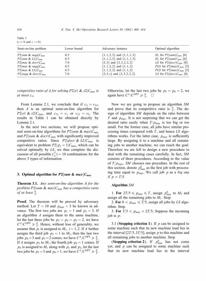
Table 1(� ¿ 0 and � → 0)

Semi-on-line problem Lower bound Adversary instance Optimal algorithm

P2|sum & sugg|Cmax 4=3 {1; 1; 2; 2} and {1; 1; 1; 3} H3 for P2|sum|Cmax [6]P2|sum & LL|Cmax 4=3 {1; 1; 2; 2} and {1; 1; 1; 3} H3 for P2|sum|Cmax [6]P2|max & decr|Cmax 7=6 {3; 3} and {3; 3; 2; 2; 2} LS for P2|decr|Cmax [8]P2|max & sugg|Cmax 4=3 {1; 1; 2; 2} and {1; 1; 2} PLS for P2|max|Cmax [5]P2|max & LL|Cmax 4=3 {1; 1; 2; 2} and {1; 1; 2} PLS for P2|max|Cmax [5]P2|sugg & decr|Cmax 7=6 {3; 3; �} and {3; 3; 2; 2; 2} LS for P2|decr|Cmax [8]

competitive ratio of A for solving P2|s1 & s2|Cmax isat most cA.

From Lemma 2.1, we conclude that if cA = c12,then A is an optimal semi-on-line algorithm forP2|s1 & s2|Cmax, and c12 = c1 or c12 = c2. Theresults in Table 1 can be obtained directly byLemma 2.1.

In the next two sections, we will propose opti-mal semi-on-line algorithms for P2|sum & max|Cmax

and P2|sum & decr|Cmax with signi<cantly improvedcompetitive ratios. Since P2|decr & LL|Cmax isequivalent to problem P2|pj = 1|Cmax, which can besolved optimally by LS, we thus complete the dis-cussion of all possible ( 5

2 ) = 10 combinations for theabove 5 types of information.

3. Optimal algorithm for P2|sum & max|Cmax

Theorem 3.1. Any semi-on-line algorithm A for theproblem P2|sum & max|Cmax has a competitive ratioof at least 6

5 .

Proof. The theorem will be proved by adversarymethod. Let T = 10 and pmax = 3 be known in ad-vance. The <rst two jobs are p1 = 1 and p2 = 3. Ifan algorithm A assigns them to the same machine;let the last three jobs be p3 = p4 = p5 = 2; we haveCA=COPT¿ 6

5 . Hence; without loss of generality; weassume that pi is assigned to Mi; i = 1; 2. If A furtherassigns the third job p3 = 1 to M2; then the last twojobs p4 =3 and p5 =2 comes; we have CA=COPT¿ 6

5 .If A assigns p3 to M1; the fourth job p4 = 1 comes. Ifp4 is assigned to M1 along with p1 and p3; let the lasttwo jobs be p5 =3 and p6 =1; we have CA=COPT¿ 6

5 .

Otherwise; let the last two jobs be p5 = p6 = 2; weagain have CA=COPT¿ 6

5 .

Now we are going to propose an algorithm SMand prove that its competitive ratio is 6

5 . The de-sign of algorithm SM depends on the ratio betweenT and pmax. It is not surprising that we can get thedesired ratio easily when T=pmax is too big or toosmall. For the former case, all jobs have similar pro-cessing times compared with T , and hence LS algo-rithms works. For the latter case, pmax is suBcientlylarge. By assigning it to a machine and all remain-ing jobs to another machine, we can reach the goal.Therefore we are left to design a new procedure todeal with the remaining cases carefully. In fact, SMconsists of three procedures. According to the valueof T=pmax; SM chooses one procedure. In the rest ofthis section, denote p0

max as the <rst job with process-ing time equal to pmax. We call job p as a big oneif p ¿ T=5.

Algorithm SM

1. For 2T=56pmax6T , assign p0max to M2 and

assign all the remaining jobs to M1. Stop.2. For 0 ¡ pmax6T=5, assign all jobs by LS algo-

rithm. Stop.3. For T=5 ¡ pmax ¡ 2T=5; Suppose the incoming

job is p.

3.1 (Stopping criterion 1). If p can be assigned tosome machine such that its new machine load lies inthe interval [2T=5; 3T=5], assign p to this machine andall remaining jobs to another machine. Stop.

(Stopping criterion 2). If p0max has not come

yet, and p can be assigned to some machine suchthat its new machine load lies in the interval

Z. Tan, Y. He / Operations Research Letters 30 (2002) 408–414 411

[2T=5−pmax; 3T=5−pmax], assign p and p0max to this

machine and all remaining jobs to another machine.Stop.

3.2. If p6T=5 or p is p0max, assign it to M1. Other-

wise, if p is a big job other than p0max, assign it to M2.

If there are already two big jobs on M2, then assignall remaining jobs to M1. Stop.

3.3. If p is not the last job, return to Step 3.

Lemma 3.2. Once one of the two Stopping criteriais satis<ed; CSM =COPT6 6

5 .

Proof. Obviously; no matter which criterion issatis<ed; the load of the machine scheduling p liesin the interval [2T=5; 3T=5]. On the other hand; theload of another machine is also no greater thanT − 2T=5 = 3T=5. Thus; CSM 6 3T=56 6COPT=5.

Theorem 3.3. SM has a competitive ratio of 65 and

is an optimal algorithm for the semi-on-line problemP2|sum & max|Cmax.

Proof. It is clear that for T=26pmax6T; SMyields an optimal schedule. For 2T=56pmax ¡ T=2;we have CSM 6T − pmax6 3T=56 6COPT=5. For0 ¡ pmax6T=5; SM assigns jobs by LS rule. As thedi=erence between the <nal loads of two machinesnever exceeds pmax; we have CSM 6 (T − pn)=2 +pn6 (T + pmax)=26 3T=56 6COPT=5. Hence weare left to consider the case of T=5 ¡ pmax ¡ 2T=5.

We prove it by contradiction. By Lemma 3.2, weonly need to consider the case where two Stoppingcriteria are not satis<ed. Note that p0

max should alwaysbe assigned to M1 for this case. Moreover, only bigjobs can be assigned to M2. If there are already twobig jobs pi1 ; pi2 on M2 before p0

max arrives, we havepi1 +pi2 ¿ 2T=5 and thus by Lemma 3.2, CSM =pi1 +pi2 ¿ 3T=5. Because pi1 6pmax; pi2 6pmax and inany optimal schedule, there exists a machine whichprocesses at least two jobs in {pi1 ; pi2 ; pmax}; SM getan optimal solution. Otherwise, by Stopping criterion2, the current load of M1 is less than 2T=5−pmax whenp0

max comes. To avoid SM assigning jobs accordingto Stopping criterion 1, two big jobs other than p0

maxmust come (Perhaps one of them comes before p0

max).Using the same method as above we can see that SMget an optimal solution.

4. Optimal algorithm for P2|sum & decr|Cmax

Theorem 4.1. Any semi-on-line algorithm A for theproblem P2|sum & decr|Cmax has a competitive ratioof at least 10

9 .

Proof. Let the total processing time of jobs be 18. Ifan algorithm A assigns the <rst two jobs p1 = p2 = 4to the same machine; the last four jobs with pro-cessing times p3 = p4 = p5 = p6 = 5

2 come; wehave CA=COPT¿ 10

9 . Otherwise; let the last four jobsare p3 = p4 = p5 = 3 and p6 = 1; we again haveCA=COPT¿ 10

9 .

Now we present an optimal algorithm SD. SD <rstassigns the <rst two jobs according to their total pro-cessing time. If the sum of these two jobs is between4T=9 and 5T=9, then SD assigns all remaining jobs toanother machine. Otherwise SD assigns all remainingjobs by LS except that the incoming job satis<es oneof the two Stopping criteria.

Algorithm SD1. Assign p1 to M1.2. For 4T=96p1 + p26 5T=9, assign p2 to M1

and the remaining jobs to M2. Stop.3. For p1 +p2 ¡ 7T=18, assign p2 to M1 and go to

Step 5.4. For 7T=186p1+p2 ¡ 4T=9 or p1+p2 ¿ 5T=9,

assign p2 to M2, go to Step 5.5. Suppose the incoming job is p.

5.1 (Stopping criterion 1). If p can be assigned tosome machine such that its new machine load lies inthe interval [4T=9; 5T=9], then assign p to this machineand all remaining jobs to another machine. Stop.

(Stopping criterion 2). If p can be assigned to themachine with minimum current load such that the newload is greater than 5T=9, assign p to this machine andall the remaining jobs to another machine. Stop.

5.2. Assign p to the machine with minimum currentload (If two machines have the same current loads,assign p to M2).

5.3. If p is not the last job, return to Step 5.

In the rest of the section, we normalize theprocessing time of all jobs in such a way thatT = 18. Thus we have Cmax¿T=2 = 9: DenotePi = {p1; : : : ; pi}; 16 i6 n.

412 Z. Tan, Y. He / Operations Research Letters 30 (2002) 408–414

Theorem 4.2. SD has a competitive ratio of 109 and

is an optimal algorithm for the semi-on-line problemP2|sum & decr|Cmax.

Proof. We will prove the theorem by contradic-tion. Assume there exists an instance such thatCSD ¿ 10COPT=9¿ 10; which implies that algorithmSD must enter Stopping criterion 2. Suppose pt isthe <rst job assigned to the machine with minimumcurrent load and the new load of this machine ex-ceeds 10 whereas both machines have load smallerthan 8 before pt arrives. Hence; pt ¿ 2. We call pt akey job. As jobs arrive in the order of non-increasingprocessing times; no machine can schedule more than3 jobs before pt arrives. We conclude t6 7. In thefollowing; we distinguish several cases with respectto the value of t. For each case; only situations whereStopping criterion 1 is not satis<ed are considered.We use (J1; J2) to denote the assignment of jobs inJ1 ∪ J2 ⊂ J in a given schedule; i.e. denote Ji to bejobs already assigned to Mi; i = 1; 2.

Case 1: t = 7.If p1 + p2 ¿ 10, then T ¿

∑7i=1 pi =(p1 + p2)+

∑7i=3 pi ¿ 10+2·5 ¿ 18, a contradiction. If 86p1+

p26 10, obviously we have CA6 10, which impliesthe desired competitive ratio. If p1 + p2 ¡ 8, we canconclude only that the following three possible assign-ments of P6 by algorithm SD should be considered:

A1: ({p1; p4; p5}; {p2; p3; p6});A2: ({p1; p2; p6}; {p3; p4; p5});A3: ({p1; p4; p6}; {p2; p3; p5}):In fact, since no machine can schedule more than 3jobs before pt arrives, we only need consider the SDassignments that each machine schedules 3 jobs of P6.Among totally 1

2 (63 ) = 10 such possible assignments,

we show that the following NA1–NA7 are impossible.

NA1: ({p1; p5; p6}; {p2; p3; p4});NA2: ({p1; p3; p4}; {p2; p5; p6});NA3: ({p1; p3; p5}; {p2; p4; p6});NA4: ({p1; p3; p6}; {p2; p4; p5});NA5: ({p1; p2; p3}; {p4; p5; p6});NA6: ({p1; p2; p4}; {p3; p5; p6});NA7: ({p1; p2; p5}; {p3; p4; p6}):If the assignment of P6 is NA1, we have p1 ¿ p2 +p3. Otherwise, p4 should be assigned to M1 in Step

5.2, a contradiction. Hence, we get p1 ¿ 4 and thusp1 + p5 + p6 ¿ 4 + 2 · 2 = 8, which violates theassumption that p7 is the key job. If the assignmentof P6 is one of NA2–NA4; p1¿p2 implies that p3

should be assigned to M2 in Step 5.2, a contradiction.If the assignment of P6 is one of NA5–NA7, we havep1 +p2 ¡ 7, which deduces that p3; p4; p5 should allbe assigned to M2 in Step 5.2, a contradiction again.We thus conclude that the assignments NA1–NA7 areimpossible. In the following we will get contradictionby considering A1, A2 and A3 separately, which cancomplete the proof of Case 1.

Subcase 1.1: The assignment of P6 is A1.In this subcase, we have CSD = min {p1 + p4 +

p5; p2 + p3 + p6}+ p7. Moreover, since p1 and p2

are not assigned to the same machine by algorithmSD, we have p1 + p2¿ 7.

Consider the assignment of P7 in an optimal sched-ule. If one machine processes at least <ve jobs, wehave COPT¿

∑7i=3 pi. If the distribution of P7 in an

optimal schedule is 4:3, it is not diBcult to verify thateither COPT¿p1 + p2 + p7, or COPT¿p2 + p5 +p6 + p7. For each case, we will show below that oneof the following two results is valid: (i) T ¿ 18, (ii)there exists i and j such that i ¿ j and pi ¿ pj. Bothare the desired contradictions.

1. COPT¿∑7

i=3 pi.By 9(p2 + p3 + p6 + p7)¿ 9CSD ¿ 10COPT¿

10∑7

i=3 pi, we have 9p2 ¿ 10(p4 +p5)+p3 +p6 +p7 ¿ 23p7¿ 46, i.e. p2 ¿ 5. Thus, T ¿

∑7i=1 pi¿

2p2 + 5p7 ¿ 20.2. COPT¿p1 + p2 + p7.We only prove the case of CSD =p1+p4+p5+p7;

the case of CSD = p2 + p3 + p6 + p7 can be provedsimilarly. It implies p1 + p4 + p56p2 + p3 + p6. Ifp4 + p56p2 + 1, then from p1 + p2 + p7 ¿ 9, wehave 9CSD = 9(p1 + p7 + p4 + p5)6 9(p1 + p7) +9(p2 +1)6 10(p1 +p2 +p7)6 10COPT. Otherwise,T ¿

∑7i=1 pi¿ 2(p1 +p4 +p5)+p7 ¿ 2(p1 +p2 +

1) + p7 ¿ 18.3. COPT¿p2 + p5 + p6 + p7.

By 9(p2 + p3 + p6 + p7)¿ 9CSD ¿ 10COPT¿10(p2 + p5 + p6 + p7), we have 9p3 ¿ 10p5 + p2 +p6 + p7. If p2 ¿ 3, then 9p3 ¿ p2 + 12p7 ¿ 27 andT ¿ (p1+p2)+p3+4p7¿ 7+3+8=18. Otherwise,9p3 ¿ p2 + 12p7¿p2 + 24¿ 9p2.

Z. Tan, Y. He / Operations Research Letters 30 (2002) 408–414 413

Subcase 1.2: The assignment of P6 is A2.Obviously, CSD=min {p1+p2+p6;

∑5i=3 pi}+p7.

If the assignment of P7 in an optimal scheduleis ({p1; p2; p3}; {p4; p5; p6; p7}), then we knowCOPT¿max {∑3

i=1 pi;∑7

i=4 pi}. Otherwise, nomatter what the distribution of P7 in an optimal sched-ule is, we have COPT¿p3 +

∑7i=5 pi. We show that

any of the above lower bounds of COPT can get thesame contradictions as Subcase 1.1.

1. COPT¿p3 +∑7

i=5 pi.Obviously, 9(

∑5i=3 pi +p7)¿ 9CSD ¿ 10COPT¿

10(p3 +∑7

i=5 pi). It follows 9p4 ¿ 10p6 + p3 +p5 + p7. If p3 ¿ 3, then 9p4 ¿ p3 + 12p7 ¿ 27 andT ¿ 4p4+3p7 ¿ 12+6=18. Otherwise, 9p4 ¿ p3+24¿ 9p3, a contradiction, again.

2. COPT¿max{∑3i=1 pi;

∑7i=4 pi}.

If∑3

i=1 pi6∑7

i=4 pi, by 9(∑5

i=3 pi + p7)¿9CSD ¿ 10COPT¿ 10

∑7i=4 pi, we have 9p3 ¿ p4 +

p5 + 10p6 + p7¿∑3

i=1 pi + 9p6¿ 3p3 + 9p6, i.e.p3 ¿ 3p6=2 ¿ 3. Then T ¿ 2

∑3i=1 pi ¿ 18.

Otherwise, 9∑3

i=1 pi ¿ 9∑7

i=4 pi =9(∑5

i=3 pi +p7)+9p6−9p3 ¿ 10

∑3i=1 pi +9p6−9p3=10(p1+

p2) + 9p6 + p3 since 9CSD ¿ 10COPT. It follows9p3 ¿ p1 + p2 + 9p6 + p3, i.e. p3 ¿ 3p6=2 ¿ 3. Onthe other hand, as 9(

∑5i=3 pi + p7) ¿ 10

∑3i=1 pi ¿

9∑3

i=1 pi +∑7

i=4 pi, we have 8(p4 + p5 + p7)¿ 9(p1 + p2) + p6. Hence, 72 = 4T ¿8∑7

i=4 pi ¿ 9(p1 +p2 +p6), i.e. p1 +p2 +p6 ¡ 8,which violates the inequality p3 ¿ 3.

Subcase 1.3: The assignment of P6 is A3.Obviously, CSD = min {p1 + p4 + p6; p2 + p3 +

p5}+ p7, the same arguments as above can show theresult. The proof of Case 1 is thus completed.

Case 2: t = 6.Using the same approach as Case 1, the possible

assignment of P5 by algorithm SD can be listed asfollows:

A4: ({p1; p5}; {p2; p3; p4});A5: ({p1; p4; p5}; {p2; p3});A6: ({p1; p4}; {p2; p3; p5}):

Subcase 2.1: The assignment of P5 is A4.We have CSD = min {p1 + p5;

∑4i=2 pi} + p6.

The distribution of P6 in an optimal schedule cannotbe 3:3 to avoid CSD6COPT. So COPT¿

∑6i=3 pi.

Moreover, if p1 + p2 ¿ 10, then T ¿ p1 + p2 +4p6 ¿ 10+8=18. So p1+p2 ¡ 8 and p16

∑4i=2 pi.

Since∑5

i=2 pi ¿ 8, we know∑5

i=2 pi ¿ 10 by Stop-ping criterion 1. Combining it with p1 + p2 ¡ 8,we have

∑5i=3 pi ¿ p1 + 2. By 9(p1 + p5 +

p6)¿ 9CSD ¿ 10COPT¿ 10∑6

i=3 pi, we have9∑5

i=3 pi ¿ 9p1 +18 ¿ 10(p3 +p4)+p5 +p6 +18.It implies 9p5 ¿

∑6i=3 pi + 18¿ 3p5 + 20, i.e.

p5 ¿ 10=3. Thus, T ¿ 5p5 + p6 ¿ 56=3 ¿ 18, acontradiction.

Subcase 2.2: The assignment of P5 is A5.We have CSD = min {p1 + p4 + p5; p2 +

p3} + p6. To avoid CSD6COPT, the only twopossible assignments of P6 in an optimal sched-ule are ({p1; p2}; {p3; p4; p5; p6}) and ({p1; p3};{p2; p4; p5; p6}). It implies COPT¿

∑6i=3 pi. If

p2 + p3 + p5 ¡ 8, then p2 + p3 + p6 ¡ 8, whichviolates the de<nition of p6. So p2 + p3 + p5 ¿ 10.If p1 ¿ 4, then T ¿ p1 + (p2 + p3 + p5) +2p6 ¿ 18. Otherwise, by 9(p1 + p4 + p5 +p6)¿ 9CSD ¿ 10COPT¿ 10

∑6i=3 pi, we have

36¿ 9p1 ¿ 10p3 + p4 + p5 + p6¿ 10p3 + 6, i.e.p3 ¡ 3. It follows p2 ¿ 10 − (p3 + p5) ¿ 4¿p1.

Subcase 2.3: The assignment of P5 is A6.Obviously, CSD = min {p1 + p4; p2 + p3 +

p5} + p6. Three possible assignments of P6

in an optimal schedule to avoid CSD6COPT

are ({p1; p2}; {p3; p4; p5; p6}); ({p1; p3}; {p2; p4;p5; p6}) and ({p1; p5; p6}; {p2; p3; p4}). Similararguments as Subcase 2.1 and Subcase 1.3 can <nishthe proof of the <rst two cases and the last one, re-spectively. We omit the detail here and Case 2 is thus<nished.

Case 3: t = 5.We only need to consider the situation that the

assignment of P4 by algorithm SD is ({p1; p4};{p2; p3}), while the possible assignments of P5 inan optimal schedule are ({p1; p2}; {p3; p4; p5})or ({p1; p3}; {p2; p4; p5}). Hence COPT¿p1 + p3

and COPT¿∑5

i=3 pi. We distinguish three subcasesaccording to the value of p1; p2 and p3.

Subcase 3.1: p1 + p3 ¿ 10.By 9(p2 +p3 +p5)¿ 9CSD ¿ 10COPT¿ 10(p1 +

p3) ¿ 100, we have p2 + p3 + p5 ¿ 11. It impliesp1 + p4 ¡ 7. Combining it with p1 + p3 ¿ 10, wehave p3 ¿ p4 + 3¿ 5 and T ¿ 3p3 + 2p5 ¿ 19, acontradiction.

414 Z. Tan, Y. He / Operations Research Letters 30 (2002) 408–414

Subcase 3.2: p1 + p2 ¿ 10 and p1 + p3 ¡ 8.Obviously, p2 ¿ p3 + 2. If COPT¿p2 + p4 + p5,

we have 9p3 ¿ p2 + p5 + 10p4 ¿ p3 + 2 + p5 +10p4, i.e. 8p3 ¿ 24. As p1+p3 ¡ 8, we have p1 ¡ 5,which violates the inequality p1 + p2 ¿ 10. Other-wise, COPT¿p1 +p2, we have 9(p3 +p5) ¿ 10p1 +p2 ¿ 9p1 + 10, i.e. p3 + p5 ¿ p1 + 1 ¿ 6. Thus,T ¿ (p1 + p2) + (p3 + p5) + p4 ¿ 18.

Subcase 3.3: p1 + p2 ¡ 8.As p5 is a key job, we have p2 + p3 + p5 ¿ 10

and thus p3 +p5 ¿ p1 +2. If p1 +p4 ¿ p2 +p3, by9(p2+p3+p5)¿ 9CSD ¿ 10COPT¿ 10

∑5i=3 pi, we

have 10p2=9p2+p2 ¿ 10p4+p3+p5+p2 ¿ 10p4+10, i.e. p2 ¿ p4 + 1. Moreover, p1 ¿ p2 + p3 −p4¿p3 + 1 and p1 + p2 ¿ p3 + p4 + 2 ¿ p3 +p5 + 2 ¿ p1 + 2 + 2. Thus p2 ¿ 4, which violatesthe inequality p1 + p2 ¡ 8. Otherwise, by 9(p1 +p4 + p5)¿ 9CSD ¿ 10COPT¿ 10

∑5i=3 pi, we have

9(p3 + p5) ¿ 9p1 + 18 ¿ 10p3 + p4 + p5 + 18. Itimplies 9p5 ¿ p3 + p4 + p5 + 18, i.e. p5 ¿ 3. More-over, 9(p2 +p3)¿ 9(p1 +p4) ¿ 10p3 +10p4 +p5.It follows 9p2 ¿ p3+10p4+p5, i.e. p2 ¿ 4p5=3=4,which violates the inequality p1 + p2 ¡ 8 again. Theproof of Case 3 is thus <nished. As the case of t6 4is trivial, the proof of Theorem 4.2 is completed.

5. Conclusions

This paper considered the semi-on-line versionsof scheduling problem P2‖Cmax. We gave a com-prehensive study on the semi-on-line versions withcombination of two types of information among<ve basic ones. For two versions among them weshowed that combination is more useful to devisesemi-on-line algorithm with smaller competitive ra-tio. The <rst is that the total processing time of alljobs and the largest processing time of all jobs areknown in advance. The second is that the total pro-cessing time of all jobs is known in advance andjobs arrive in order of non-increasing processing

times. We presented their respective optimal algo-rithms with competitive ratio 6

5 and 109 , respectively.

For the remaining versions, we can conclude from Ta-ble 1 which type of information is not necessary whileanother one is already available.

Acknowledgements

The authors would like to acknowledge the com-ments by the referee which have improved the presen-tation of the paper.

References

[1] Y. Azar, O. Regev, Online bin stretching, Proceedings of theRANDOM’98, Barcelona, Spain, 1998, pp. 71–82.

[2] B. Chen, C.N. Potts, G. Woeginger, A review of machinescheduling: Complexity, algorithms and approximability, in:D.-Z. Du, P.M. Pardalos (Eds.), Handbook of CombinatorialOptimization, Kluwer Academic Publishers, Dordrecht, 1998.

[3] Y. He, The optimal on-line parallel machine scheduling,Comput. Math. Appl. 39 (2000) 117–121.

[4] Y. He, Z. Tan, Ordinal online scheduling for maximizingthe minimum machine completion time, J. Combin. Optim.6 (2002) 199–206.

[5] Y. He, G.C. Zhang, Semi on-line scheduling on two identicalmachines, Computing 62 (1999) 179–187.

[6] H. Kellerer, V. Kotov, M.G. Speranza, Z. Tuza, Semi on-linealgorithms for the partition problem, Oper. Res. Lett. 21(1997) 235–242.

[7] W.P. Liu, J.B. Sidney, A. van Vliet, Ordinal algorithmsfor parallel machine scheduling, Oper. Res. Lett. 18 (1996)223–232.

[8] S. Seiden, J. Sgall, G. Woeginger, Semi-online schedulingwith decreasing job sizes, Oper. Res. Lett. 27 (2000)215–227.

[9] D. Sleator, R.E. Tarjan, Amortized eBciency of list updateand paging rules, Commun. ACM 28 (1985) 202–208.

[10] Z. Tan, Y. He, Semi-on-line scheduling with ordinal data ontwo uniform machines, Oper. Res. Lett. 28 (2001) 221–231.

[11] Z. Tan, Y. He, Ordinal algorithms for parallel machinescheduling with nonsimultaneous machine available times.Comput. Math. Appl., to appear.

[12] G.C. Zhang, D.S. Ye, A note on on-line scheduling withpartial information, Comput. Math. Appl., to appear.