Int. J. Dynam. ControlDOI 10.1007/s40435-016-0288-0

Semi-global output feedback nonlinear stabilization of variablespeed grid connected direct drive wind turbine generator systems

Ali Abdul Razzaq Al Tahir1

Received: 3 May 2016 / Revised: 15 November 2016 / Accepted: 17 November 2016© The Author(s) 2016. This article is published with open access at Springerlink.com

Abstract The goal of the present work is to achieve non-linear semi-global output feedback stabilization of variablespeed grid connected direct drive wind turbine generatorDDWTG systems under wind energy conversion systems toprovide the electricity demand for electrical networks. Thestudy will address the sensorless control of variable speedwind energy generation systems, namely optimized rotorspeed and direct-axis current control to determine the mostappropriate structure and to improve both robustness and reli-ability of this kind of distributed generators. The proposednonlinear observer is robust with respect to measurementserror and perturbations of the sampling schedule. The sim-ulation results of the case study support the presented maintheorem that reflects the effect of measurement errors andthe improvement with respect to global convergence prop-erties. The novelty of the present study resides in takinginto account the difficulties and control problem complex-ity that faced the nonlinear output feedback control undergo:

Preliminaries and NotationsThroughout this paper, |.| means the absolute value. Let us consider

Rdef= (−∞,∞), R+ def= (0, ∞) positive real number space, R+

0 =[0,∞], and let us define ||.|| be the Euclidean norm or the inducedmatrix norm. For p, q, n, m ∈ N , set of natural numbers, R p×q

represents the set of real matrices of order p × q and Ip ∈ I R p×p

stands for the identity matrix of order p × p. The notation ||P||, forP ∈ R p×q , represents the L2-norm of P and X T , represent thetransposed vector of X. One say that α In ≤ P ≤ β In whereP ∈ Rn×n if, λmin (P) ≥ α and λmax (P) ≥ β where λmin (.) andλmax (.) denote, respectively the smallest and the biggesteigenvalues of the square matrix. In all this study, the initialboundary time is called t0 ∈ [0, ∞).

B Ali Abdul Razzaq Al Tahirrazzaqali2007@yahoo.com; ali.altahir@uokerbala.edu.iq

1 Electrical Engineering Department, College of Engineering,University of Kerbala, Ministery of Higher Education andScientific Research, Kerbala, Iraq

(i) the proposed system nonlinearity and loss the observ-ability of sensorless PMSG near the singularity point of therotor speed; (ii) inaccessibility measurements for all systemstate variables; (iii) maximum power point tracking of opti-mum reference angular rotor speed; (IV) magnetizing anddemagnetizing direct-axis current at standstill; (V) the pro-posed semi-global observer has dynamic high-gain designparameter DHGO. The simulation results of variable speedgrid connected DDWTG, in general, confirm the main theo-remdeveloped underDHGOparameter and lead us to enlargeand prolongation the admissible sampling period using non-linear Lyapunov stability control techniques.

Keywords AC/DC/AC double converters · MPPT · Semi-global observer · Sampled measurements · Backsteppingcontrol · Lyapunov stability tools

List of symbols

Ra Resistance of armature windings for PMSG(�)

La Armature winding inductance for PMSG (H)Vgα, Vgβ α–β axis of wind turbine generator voltage (V)Igα, Igβ α–β axis of wind turbine generator current (A)ωg Angular velocity of the generator rotor (rad/s)Tm External input mechanical torque (Nm)p Number of pole pairsJ Total inertia of the WTG rotor (Nm/rad/ss)F Total viscous friction ofWTGrotor (Nm/rad/s)θm Mechanical rotor position angle (rad)ψP M Permanent Magnent flux constant (Wb)Cbus DC link capacitor (F)Pm Mechanical output power (W)ρ Air density (1.225) (kg/m3)

123

A. A. R. Al Tahir

C p The power coefficient (unit less)C f il Capacitance of LCL filter (F)A The swept area of the turbine blade (m2)Vw The wind speed velocity (m/s)D The rotor diameter (m)L f il Inductance of LCL filter (H)

1 Introduction

Recently, wind energy is a promised energy for the com-ing years and pollution-free energy, which can help us toreduce the carbon emissions. Also, it will reduce the elec-tricity bill for household operations. Wind energy reducesnational reliance on carbon-based fuels, and it will decreasethe production of greenhouse gas emissions that will reflectpositive effects on environments, limits the pollution andtackle climate change, in the world. DDWTG can be usedto generate electricity in remote location such as mountainsand remote countryside [1].

Although, several works deal with wind turbine sim-ulator have been done in the past few years. They havebeen some studies on wind turbine simulator based onDC generators, inductions generators and permanent mag-net synchronous generators. Moreover, to avoid the need oftach generators and differentiation of rotor position and toguarantee redundancy of information, few solutions havebeen suggested to observe simultaneously the states tra-jectories, perturbation and all mechanical and electricalparameters [2].

A new variable speed wind energy control system witha permanent magnet synchronous generator and impedancesource inverter has been proposed in [3]. Characteristics ofimpedance source inverter are used for maximum powerpoint tracking control and delivering power to the grid simul-taneously. Two control methods are proposed for deliveringpower to the grid: capacitor voltage control and DC- busvoltage control. The maximum power point tracking MPPTalgorithmused in thismethod is basedon relationbetween theDC voltage and the generator speed. In the WECS, wind tur-bine can operatewith either variable speed or fixed speed. Forfixed speedwind generation system, because of the generatoris directly connected to the grid, the turbulence of the windwill result in power variations, and so affect the power qual-ity in the grid, whereas for variable speed generation system,the generator is controlled by power electronic converter. So,variable speed wind energy conversion systems have manyadvantages over fixed speed generation, such as maximumpower point tracking control method, increased power cap-ture, power quality, improved efficiency and they can be con-trolled in order to reduce aerodynamic noise and mechanicalstress.

With the development of power electronics technology,it’s possible to control the rotor speed, to increase windenergy production and to reduce drive train loads. Thus thevariable speedwind turbine generator system is becoming themost important and fastest growing application of wind gen-eration system. The use of the PMSG is becoming more andmore common for several reasons such as: very high torquecan be achieved at low speeds because PMSG is connecteddirectly to the turbine without gearbox; lower operationalnoise is achieved; no significant losses are generated in therotor and external excitation current is not needed. So, theefficiency of a PMSG basedWECS has been assessed higherthan other generators and PMSG is an attractive choice forvariable-speed generation system. In the case of PMSGbasedWECS, because of the advance of power electronic technol-ogy, decreasing equipment costs [4].Wind power productionhas been under the main focus for the past decade in powerproduction and tremendous amount of researchwork is goingon renewable energy, specifically on wind power extraction.Wind power provides an eco-friendly power generation andhelps to meet the national energy demand when there is adiminishing trend in terms of non-renewable resources. Asalready mentioned, mechanical sensors based solutions aremost costly and unreliable. Then, state observers turn out tobe a quite natural alternative to get estimates of mechanicalvariables using only measurable electrical state variables [5].

There are many literatures concerning with the design ofcontinuous-time high gain observers for example as in [6],the authors proposed a global observer with the global Lip-schitz condition of the system. Nevertheless, this assumptionis removed through the Lipschitz extension technique whenthe semi-global observer is proposed. For continuous-timesystems introduced by [7–9] are designed in order to addressthe issue of the sensitivity to measurements error inherentto these kinds of observers. A robust high-gain observer fornonlinear systems to provide a solution to the noise sensitiv-ity of high-gain observers, which behaves well with respectto noise and the high gainExtendedKalmanFilter EKF that isperformant with respect to large perturbations, was proposedby [10].

Several studies had been addressed the problemof control-ling power generation in variable speed wind turbines, suchas sliding mode control and backstepping control strategieshave been proposed to ensure stable operation in differentoperating regions [11–13]. Many nonlinear control tech-niques have been proposed, such as fuzzy logic-control,backstepping control technique, differential Flatness basedcontrol, and sliding mode control. However, most of theabove works need continuous-time measurements of the ACvoltages, the AC-currents, and the dc-voltage. This requiresmany of voltage and current sensors, whichwill increase sys-tem complexity, cost, space and reduces system reliability ofoperation.

123

Semi-global output feedback nonlinear stabilization of variable speed grid connected direct. . .

A simple control strategy for the operation of a variablespeed stand-alone wind turbine with a permanent magnetsynchronous generator (PMSG) to meet maximum powerextraction from the available wind power through DC–DC bidirectional buck-boost converter, which is connectedbetween batteries bank and DC-link voltage, is used to main-tain the DC-bus voltage at a constant value claimed by [14].Existing MPPT methods can be separated in two categories.The first one includesmethods based on the explicit use of thewind turbine power characteristics, which necessitate onlinemeasurements of wind velocity and (turbine/PMSG) rotorvelocity [15]. In fact, the required wind velocity measure-ment is a kind of average value of wind velocity along theturbine blade which is not easy to measure. This drawback isovercome in [16]where the proposedMPPTmethod involvesa Kalman predictor estimating the load/turbine torque basedon rotor speed measurements. The whole control design,including the Kalman predictor, is based on a linear approxi-mation of the wind turbine systems and no formal analysis ismade therefor the proposed control strategy was not proved.The second category of MPPT methods, using perturbationobservation technique, without needing turbine characteris-tics as provided in [17,18]. These methods are most suitablefor small scale wind turbine generator systems.

Output feedback control using high-gain observers aswell as measurement noise for a class of nonlinear sys-tems was provided by [19], A brief introduction to high-gainobservers in nonlinear feedback control introduced by [20],with emphasis on the peaking phenomenon and the roleof control saturation in dealing with it. The paper surveysrecent results on the nonlinear separation principle, condi-tional servo compensators, extended high-gain observers,performance in the presence of measurement noise andsampled-data control. A semi-global stabilization throughoutput-feedback for a class of uncertain nonlinear systemswas presented by [21]. An output-feedback controller is con-structed for the systemswith the appropriate choice of designparameters; this controller can make the closed-loop systemglobally attractive and semi-globally exponentially stable atthe region of attraction.

In this study, semi-global sampled high-gain observerdesign having dynamic HGO parameter is proposed to getonline estimates of the generator rotor speed, rotor positionangle and external input generator torque from the mea-surements of stator voltages and output currents. The rotorposition is derived from the estimated rotor fluxes in (α–β)stationary reference frame without needing initial rotor posi-tion detection. The major contributions of this work can besummarized as follows:

1. The successful construction of mathematical model ofa variable speed grid connected direct drive wind tur-

bine generator system and integrated it to the electricalnetworks.

2. Maximum power point extraction for best generator rotorangular speed.

3. On line estimation of the mechanical states variables,which are rotor angular speed, aerodynamic generatortorque, taking into accounts the electrical variables (out-put currents and input control voltages) are accessible formeasurements.

4. Estimation of rotor position anglewhenever the estimatesof the rotor fluxvector [ψrα, ψrβ ]T in stationary referenceframe become available.

5. Best selection of direct-axis stator current component toensure cancelation of reluctance torque and provide themaximum torque i.e., regulating the current id to tracka reference value idre f . With this control, the generatortorque is coordinated with the q-axis current,

6. Regulation of DC bus voltage, control of active and reac-tive power, and satisfying unity power factor correctionunder variable speed wind condition.

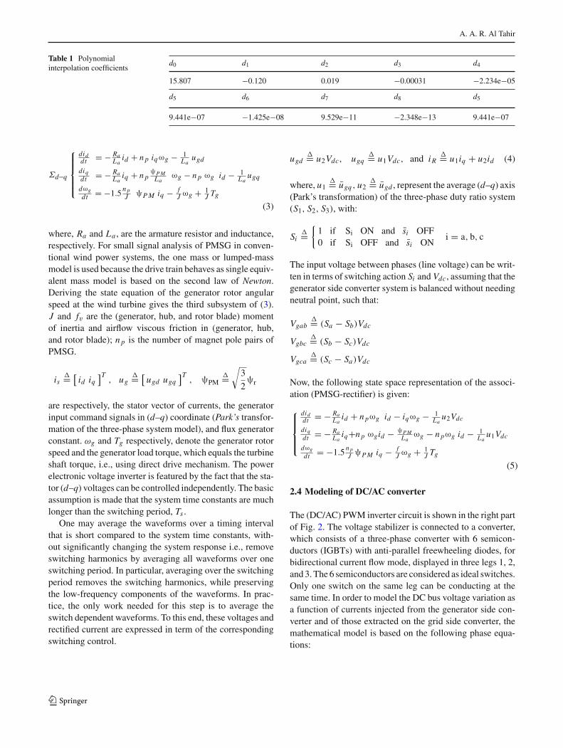
One of the challenges faced this work that the electromag-netic torque is not direct output injected and another difficultythat the stator and rotor current vector is inaccessible to mea-surements all the time. Only sampled-data measurementsare presently available at each sampling instant. This paperwill focus on the generating system shown in Fig. 2, whichconsists of a PMSG that converts wind power into outputvoltage whose amplitude and frequency vary accordinglywith wind velocity. The three-phase variable frequency, volt-age generated from the wind turbine is rectified using arectifier-inverter (AC/DC/AC) IGBT PWM converter), con-nected through a DC bus power transfer. The AC side of therectifier is connected to the PMSG stator, the inverter DC/ACoutput is tied to the electrical grid via an inductive filter thatperforms the filtering of current harmonics due to the inverterswitching actions. The PMSG is controlled through the abovepower converter that switches the phases depending on thegenerator rotor position. An observer based on sampled-datamechanism is used to reconstruct the rotor speed actuatorand the control laws are reconfigured using the estimatedstate information.

This paper is organized as follows. Section 2 introducesthe mathematical model for variable speed DDWT system,Sect. 3 presents state feedback nonlinear controller designobjectives. Section 4 deals with DC voltage regulator andreactive power control. Section 5 focuses on semi-global out-put feedback nonlinear controller design; meanwhile, Sect. 6stability convergence analysis of the proposed semi-globalsampledHGOobserver are discussed. Simulation results andverifications are shown in Sect. 7. Finally, the conclusion andremarks are drawn in Sect. 8.

123

A. A. R. Al Tahir

2 Mathematical formulation for variable speedDDWTG

2.1 Modeling of wind turbine

Some of wind turbines do not contain a gearbox andinstead use a direct drive mechanism to produce powerfrom the generator, which converts the aerodynamic energyto mechanical, electric energy and delivers it to the dis-tribution system. As the wind velocity varies, the powercaptured which converted and transmitted to electricalsload also varies [22]. The transmitted power is generallydeduced from the wind power, using the power coefficientC p as:

Pm = 0.5 ρ A C pV 3w

C p = c1 ×(

c21

λ0− c3θp − c4

)e−c5

1

λ0+ c6λ

λ = Rωr

Vw

,1

λ0= 1

λ + 0.08θp− 0.035

1 + (θ p)3 (1)

Vw = Vb + Vg + Vr + Vnoise

where, Pm is the mechanical output power in watt, the airdensity ρ in kg/m3. C p (called the power coefficient or windturbine efficiency), is a nonlinear function of tip speed ratioλ = Rωr/Vw, unit less, A = π D2/4 is the swept andrecovered area of the wind turbine blades in m2, D is rotordiameter in m, and Vw is the wind velocity (m/s). With aero-dynamic wind turbine coefficients, c1, c2, c3, c4, c5 and c6.Wind model chosen for this study is consists of four compo-nents of wind speed (m/s), which are, Vb, Vg, Vr and Vnoise.The base component is a constant speed and wind gust com-ponent can be usually represented as a sinusoidal function.The noise component may occur from wind acceleration andturbulence.

Wind turbine comprises of the blades and nacelle. Thenacelle houses, electrical control systems, mechanical brake,electromagnetic brake and the PMSG. The blades drive thegenerator round which generates the electricity. Inverter asthe voltage from the generator is different to that of the grid;the power from the generator needs to be converted to DC.The inverter then changes the output ensuring it is suit ablefor the local grid system [23]. The ideal power curve exhibitsthree different regions with distinctive generation objectives.At lowwind velocity region, the available power is lower thanrated power. The available power is defined as the power inthe wind passing through the rotor area multiplied by thebest power coefficient; C p−opt (λ, β) < 1. So, the gener-ation objective in first region is to extract all the availablepower. Therefore, the ideal power curve in this region fol-lows a cubic parabola defined by system (1). On the otherhand, the generation goal in the high wind velocity is to

limit the generated power below its rated value to avoid overloading.

In this region, the available power exceeds rated power;therefore the wind turbine must be operated with efficiencylower thanC p−opt . Finally, second region is actually a transi-tion between the optimum power curve of first region and theconstant power line of third region. In second region, rotorspeed is limited to maintain acoustic noise emission withinadmissible levels and to keep centrifugal forces below valuestolerated by the rotor.

2.2 Sensorless speed reference optimization approach

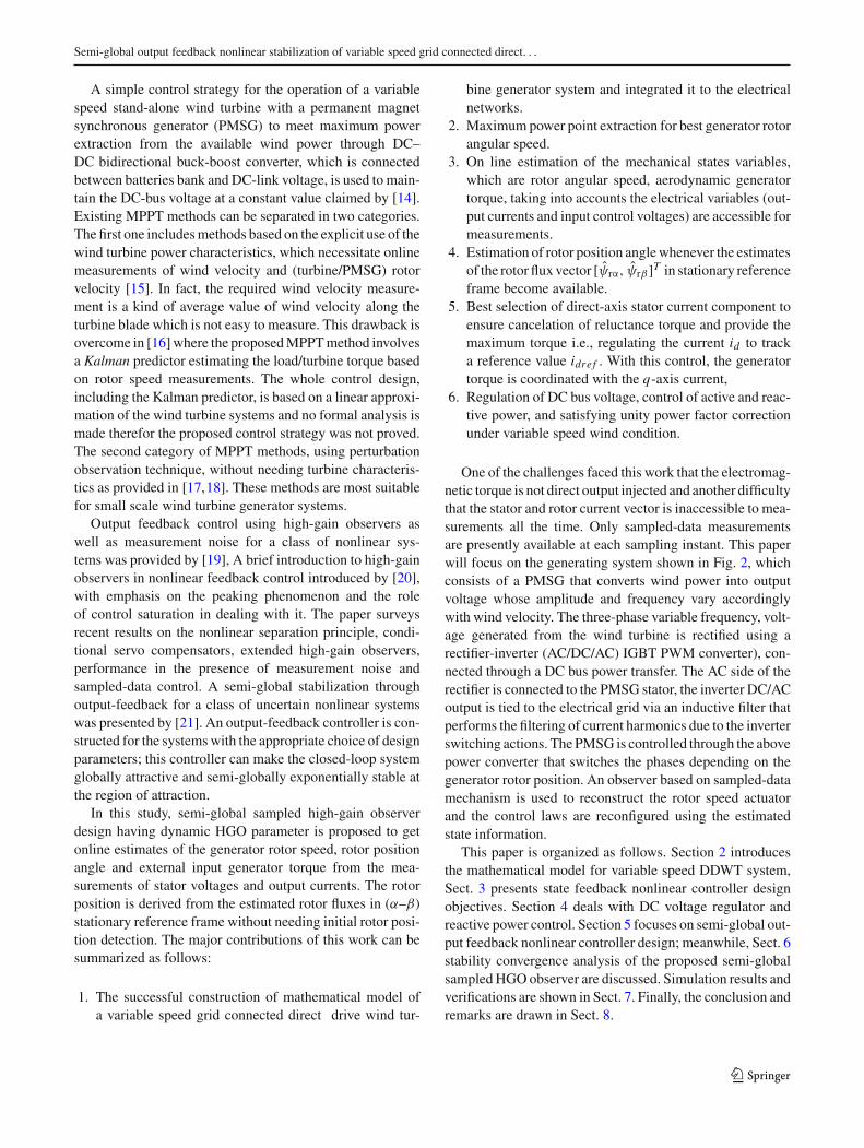
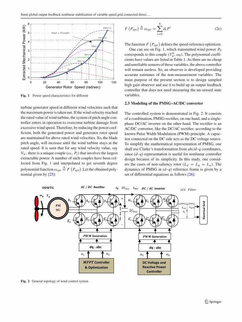
This study is looking for maximizing DDWTG efficiencyat low wind velocity; the PMSG will be connected to theblades through a MPPT controller and optimization systeminstead of step-up gear box that will help us to overcomethe cyclic maintenance for gear box. Specifically, the opti-mizer is expected to compute online the best speed valueωopt so that, if the turbine rotor speed ω is made equal toωopt then, maximal wind energy is captured, and transmit-ted to the circuit utility throughout wind turbine generatorWTG [24]. The speed-reference optimizer design is basedon the turbine power characteristic and features the fact thatit does not require wind velocity measurement. Figure 1,demonstrates turbine mechanical power versus rotor speedfor variable wind velocities. The aerodynamic behavior of awind turbine is described by the power coefficient curve C p,so that it must be defined for each wind turbine. Structure ofwind energy conversion system using PMSG is described inFig. 2, which operates according to the well-known PWMfundamental. A coupling LCL filter is used to connect thegrid side converter to the electrical grid. The aerodynamicbehavior of a wind turbine is described by the power coef-ficient curve C p, so that it must be defined for each windturbine. Structure of wind energy conversion system usingPMSG is described in Fig. 1, which operates according tothe well-known PWM fundamental. Thus, when the windvelocity changes, the speed of PMSG is controlled to fol-low the maximum power point trajectory and, the optimumrotational speed of the generator can be simply estimated asfollows:

ωopt = Vwλopt

D/2(2a)

The optimum extracted power curve from WTG is definedas:{

Popt = Koptω3opt i f Vw < Vrated

Popt = 7.5 kW i f Vw ≥ Vrated(2b)

Consequently, the MPPT sensorless control evaluates thebest wind velocity of PMSG and then regulating the wind

123

Semi-global output feedback nonlinear stabilization of variable speed grid connected direct. . .

Generator Rotor Speed (rad/sec)0 20 40 60 80 100 120

Ext

ract

ed M

echa

nica

l Pow

er (k

W)

0

1

2

3

4

5

6

Fig. 1 Power speed characteristics for different

turbine generator speed in different wind velocities such thatthemaximumpower is taken out. If thewind velocity reachedthe rated value ofwind turbine, the system of pitch angle con-troller enters in operation to overcome turbine damage fromexcessivewind speed.Therefore, by reducing the power coef-ficient, both the generated power and generator rotor speedare maintained for above rated wind velocities. So, the bladepitch angle, will increase until the wind turbine stays at therated speed. It is seen that for any wind velocity value, sayVw, there is a unique couple (ωi , Pi ) that involves the largestextractable power. A number of such couples have been col-lected from Fig. 1 and interpolated to get seventh degree

polynomial functionωopt�= F

(Popt

). Let the obtained poly-

nomial given by [25]:

F(Popt

) �= ωopt =8∑

i=0

di Pi (2c)

The function F(Popt

)defines the speed-reference optimizer.

One can see on Fig. 1, which transmitted wind power P0

corresponds to this couple (V 0w, ω0). The polynomial coeffi-

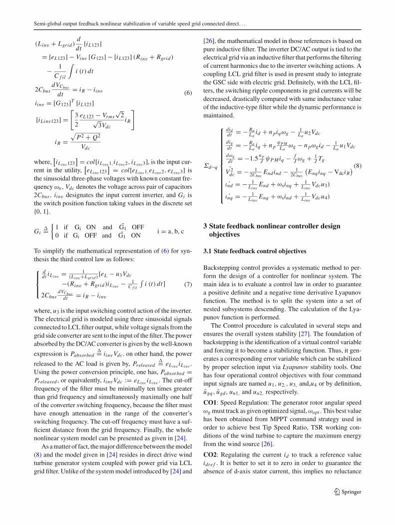
cients have values are listed in Table 1. As there are no cheapand unreliable sensors of these variables, the above controllerwill remain useless. So, an observer is developed providingaccurate estimates of the non-measurement variables. Themain purpose of the present section is to design sampledhigh gain observer and use it to build up an output feedbackcontroller that does not need measuring the un-sensed statevariables.

2.3 Modeling of the PMSG–AC/DC converter

The controlled system is demonstrated in Fig. 2. It consistsof a combination, PMSG-rectifier, on one hand, and a single-phase DC/AC inverter on the other hand. The rectifier is anAC/DC converter, like the DC/AC rectifier, according to theknown Pulse Width Modulation (PWM) principle. A capac-itor connected on the DC side acts as the DC voltage source.To simplify the mathematical representation of PMSG, oneshall use Clarke‘s transformation from abc/d–q coordinates,since (d–q) representation is useful for nonlinear controllerdesign because of its simplicity. In this study, one consid-ers the cases of non-saliency rotor (Ld = Lq = La). Thedynamics of PMSG in (d–q) reference frame is given by aset of differential equations as follows [26]:

Fig. 2 General topology of wind control system

123

A. A. R. Al Tahir

Table 1 Polynomialinterpolation coefficients

d0 d1 d2 d3 d4

15.807 −0.120 0.019 −0.00031 −2.234e−05

d5 d6 d7 d8 d5

9.441e−07 −1.425e−08 9.529e−11 −2.348e−13 9.441e−07

Σd–q

⎧⎪⎪⎪⎨⎪⎪⎪⎩

diddt = − Ra

Laid + n p iqωg − 1

Laugd

diqdt = − Ra

Laiq + n p

ψP MLa

ωg − n p ωg id − 1La

ugq

dωgdt = −1.5

n pJ ψP M iq − f

J ωg + 1J Tg

(3)

where, Ra and La , are the armature resistor and inductance,respectively. For small signal analysis of PMSG in conven-tional wind power systems, the one mass or lumped-massmodel is used because the drive train behaves as single equiv-alent mass model is based on the second law of Newton.Deriving the state equation of the generator rotor angularspeed at the wind turbine gives the third subsystem of (3).J and fv are the (generator, hub, and rotor blade) momentof inertia and airflow viscous friction in (generator, hub,and rotor blade); n p is the number of magnet pole pairs ofPMSG.

is�= [ id iq

]T, ug

�= [ ugd ugq]T

, ψPM�=√3

2ψr

are respectively, the stator vector of currents, the generatorinput command signals in (d–q) coordinate (Park’s transfor-mation of the three-phase system model), and flux generatorconstant. ωg and Tg respectively, denote the generator rotorspeed and the generator load torque, which equals the turbineshaft torque, i.e., using direct drive mechanism. The powerelectronic voltage inverter is featured by the fact that the sta-tor (d–q) voltages can be controlled independently. The basicassumption is made that the system time constants are muchlonger than the switching period, Ts .

One may average the waveforms over a timing intervalthat is short compared to the system time constants, with-out significantly changing the system response i.e., removeswitching harmonics by averaging all waveforms over oneswitching period. In particular, averaging over the switchingperiod removes the switching harmonics, while preservingthe low-frequency components of the waveforms. In prac-tice, the only work needed for this step is to average theswitch dependent waveforms. To this end, these voltages andrectified current are expressed in term of the correspondingswitching control.

ugd�= u2Vdc, ugq

�= u1Vdc, and iR�= u1iq + u2id (4)

where, u1�= ugq , u2

�= ugd , represent the average (d–q) axis(Park’s transformation) of the three-phase duty ratio system(S1, S2, S3), with:

Si�={1 if Si ON and si OFF0 if Si OFF and si ON

i = a, b, c

The input voltage between phases (line voltage) can be writ-ten in terms of switching action Si and Vdc, assuming that thegenerator side converter system is balanced without needingneutral point, such that:

Vgab�= (Sa − Sb)Vdc

Vgbc�= (Sb − Sc)Vdc

Vgca�= (Sc − Sa)Vdc

Now, the following state space representation of the associ-ation (PMSG-rectifier) is given:

⎧⎪⎪⎨⎪⎪⎩

diddt = − Ra

Laid + n pωg id − iqωg − 1

Lau2Vdc

diqdt = − Ra

Laiq+n p ωgid − ψP M

Laωg − n pωg id − 1

Lau1Vdc

dωgdt = −1.5 n p

J ψP M iq − fJ ωg + 1

J Tg

(5)

2.4 Modeling of DC/AC converter

The (DC/AC) PWM inverter circuit is shown in the right partof Fig. 2. The voltage stabilizer is connected to a converter,which consists of a three-phase converter with 6 semicon-ductors (IGBTs) with anti-parallel freewheeling diodes, forbidirectional current flow mode, displayed in three legs 1, 2,and 3. The 6 semiconductors are considered as ideal switches.Only one switch on the same leg can be conducting at thesame time. In order to model the DC bus voltage variation asa function of currents injected from the generator side con-verter and of those extracted on the grid side converter, themathematical model is based on the following phase equa-tions:

123

Semi-global output feedback nonlinear stabilization of variable speed grid connected direct. . .

(Linv + Lgrid)d

dt[iL123]

= [eL123] − Vinv [G123] − [iL123] (Rinv + Rgrid)

− 1

C f il

∫i (t) dt

2CbusdVCbus

dt= iR − iinv

iinv = [G123]T [iL123]

[iLinv123] =[3

2

eL123 − Vrms√2√

3VdciR

]

iR =√

P2 + Q2

Vdc

(6)

where,[iLinv123

] = col[iLinv1,iLinv2, iLinv3], is the input cur-rent in the utility,

[eLinv123

] = col[eLinv1,eLinv2, eLinv3] isthe sinusoidal three-phase voltages with known constant fre-quency ωn, Vdc denotes the voltage across pair of capacitors2Cbus, iinv designates the input current inverter, and Gi isthe switch position function taking values in the discrete set{0, 1}.

Gi�={1 if Gi ON and G1 OFF0 if Gi OFF and G1 ON

i = a, b, c

To simplify the mathematical representation of (6) for syn-thesis the third control law as follows:

⎧⎪⎨⎪⎩

ddt iLinv

= 1(Linv+Lgrid )

[eL − u3Vdc

−(Rinv + Rgrid)iLinv− 1

C f il

∫i (t) dt]

2CbusdVCbus

dt = iR − iinv

(7)

where, u3 is the input switching control action of the inverter.The electrical grid is modeled using three sinusoidal signalsconnected toLCLfilter output, while voltage signals from thegrid side converter are sent to the input of the filter. The powerabsorbed by theDC/AC converter is given by thewell-known

expression is Pabsorbed�= iinvVdc. on other hand, the power

released to the AC load is given by, Preleased�= eLinv

iLinv.

Using the power conversion principle, one has, Pabsorbed =Preleased , or equivalently, iinvVdc := eLinv

iLinv. The cut-off

frequency of the filter must be minimally ten times greaterthan grid frequency and simultaneously maximally one halfof the converter switching frequency, because the filter musthave enough attenuation in the range of the converter’sswitching frequency. The cut-off frequency must have a suf-ficient distance from the grid frequency. Finally, the wholenonlinear system model can be presented as given in [24].

As amatter of fact, themajor difference between themodel(8) and the model given in [24] resides in direct drive windturbine generator system coupled with power grid via LCLgrid filter. Unlike of the systemmodel introduced by [24] and

[26], the mathematical model in those references is based onpure inductive filter. The inverter DC/AC output is tied to theelectrical grid via an inductive filter that performs the filteringof current harmonics due to the inverter switching actions. Acoupling LCL grid filter is used in present study to integratethe GSC side with electric grid. Definitely, with the LCL fil-ters, the switching ripple components in grid currents will bedecreased, drastically compared with same inductance valueof the inductive-type filter while the dynamic performance ismaintained.

Σd–q

⎧⎪⎪⎪⎪⎪⎪⎪⎪⎪⎪⎪⎪⎪⎨⎪⎪⎪⎪⎪⎪⎪⎪⎪⎪⎪⎪⎪⎩

diddt = − Ra

Laid + n piqωg − 1

Lau2Vdc

diqdt = − Ra

Laiq + n p

ψP MLa

ωg − n pωgid − 1La

u1Vdc

dωgdt = −1.5 n p

J ψP Miq − fJ ωg + 1

J Tg

˙V 2dc = − 1

2CbusEndind − 1

2Cbus

(Enqinq − VdciR

)˙ιnd = − 1

LinvEnd + ωsinq + 1

LinvVdcu3)

˙ιnq = − 1Linv

Enq + ωsind + 1Linv

Vdcu4)

(8)

3 State feedback nonlinear controller designobjectives

3.1 State feedback control objectives

Backstepping control provides a systematic method to per-form the design of a controller for nonlinear system. Themain idea is to evaluate a control law in order to guaranteea positive definite and a negative time derivative Lyapunovfunction. The method is to split the system into a set ofnested subsystems descending. The calculation of the Lya-punov function is performed.

The Control procedure is calculated in several steps andensures the overall system stability [27]. The foundation ofbackstepping is the identification of a virtual control variableand forcing it to become a stabilizing function. Thus, it gen-erates a corresponding error variable which can be stabilizedby proper selection input via Lyapunov stability tools. Onehas four operational control objectives with four commandinput signals are named u1, u2,, u3, and,u4 or by definition,ugq , ugd , un1, and un2, respectively.

CO1: Speed Regulation: The generator rotor angular speedωg must track as given optimized signal,ωopt . This best valuehas been obtained from MPPT command strategy used inorder to achieve best Tip Speed Ratio, TSR working con-ditions of the wind turbine to capture the maximum energyfrom the wind source [26].

CO2: Regulating the current id to track a reference valueidre f . It is better to set it to zero in order to guarantee theabsence of d-axis stator current, this implies no reluctance

123

A. A. R. Al Tahir

torque.Only the q-axis reactance is involved in producing thefinal voltage, i.e., there is no direct magnetization or demag-netization of d-axis, only the field windings contribute toproduce the flux along this direction [28].

CO3: Ensuring a satisfactory power factor correction (PFC)at the (grid-DDWTG) connection. The inverter output cur-rents (iLinv1,iLinv2,iLinv3) must be sinusoidal with the samefrequency.

CO4: Ensuring a tight regulation of the DC output voltagedespite of wind acceleration and turbulence.

3.2 State feedback speed regulation design

For eachwind velocity, there is best TSR that keeps the powercoefficient at its best value. In order to achieve the best nom-inal TSR, it is required to control rotor speed follows bestrotor speed, which can be produced by either measuring orestimatingwind velocity. The speed regulator design is basedon second and third equation of system (3), where the inputcontrol signal usq represents the q-axis actual input, using thefollowing backstepping design technique [29] to ensure anaccurate optimized rotor speed tracking that leads us to opti-mize the capture wind energy equivalent to reference rotorspeed.

Step 1: Let us define the following generator rotor angular

speed tracking error is εω�= ωg − ωopt

In view of third equation of system (3), the above errorwill submit to the following equation:

εω = dωg

dt− ωopt = −1.5

n p

JψPMiq − f

Jωg

+ 1

JTg − ω·

opt (9)

According to (9), the design parameter: ρ = −1.5 n pJ ψPMiq ,

stands up as a virtual control input for first error dynamics,εω.

Let us consider ρre f denotes the stabilizing function con-cerning to ρ. It is readily observed from (9) that, if ρ = ρre f

with:

ρre f�= −h1εω + f

Jωg − 1

JTg + ε·

opt (10)

with h1 is positive design parameter. As a matter of fact, ifρ = ρre f , one has εω = −h1εω, which readily is asymptoti-cally stable with respect to the Lyapunov function:

W1 (εω)�= 1

2ε2ω (11)

Then take the time derivative along (8), yields

W1 (εω) = −εωεω < 0 (12)

As, ρ = −1.5 n pJ ψPMiq is just a virtual control input, one

cannot consider, ρ = ρre f .However, the above expression of ρre f is considered as

first stabilizing function and a new error is presented by:

εq�= ρ − ρre f = −1.5

n p

JψPMiq + 1.5

n p

JψPMiqre f

εq�= (iqre f − iq)

3n p

JψPM (13)

Using systems (10)–(13), it follows from (9) the first errordynamics is, εω:

εω = −h1εω + εq (14)

Step 2: The next step composite of determining the firstcontrol input u1, such that the error system (εω, εq) is asymp-totically stable. Let us get the trajectory of error, εq . The timederivative εq along the closed-loop trajectory of (13):

εq = ρ − ˙ρre f = −1.5n p

JψPM ιq + 1.5

n p

JψPM ιqre f (15)

Substituting the right hand side of (8), with aid of second andthird equation of system (5) in (15), one can obtain:

εq = ξ(id , iq,ωg

)− h21εω + h1εq + n p

JψPMu1Vdc (16)

with, ξ(id , iq,ωg

)is a nonlinear function defined in form:

ξ(id , iq,ωg

) �= n p

JψPM

(1.5

Ra

Laiq+n pωgid − n p

LaψPMωg

)

+(

f

J

)2

ωg + f n p

J 2ψPMiq − f Tg

J 2 + 1

JTg − ¨ρre f (17)

The error dynamics (14) and (16) are given the compact form:

εω = −h1εω + εq (18a)

εq = ξ(id , iq,ωg

)−h21εω + h1εq + n p

JψPMu1Vdc

(18b)

To compute stabilization control law for (18b); let us definethe quadratic Lyapunov function candidate:

W2(εω, εq

) �= W3 (εω) + 1

2ε2ω (19)

In view of (12), the time derivative of W2(εω, εq

)along the

trajectories can be rewritten as:

W2(εω, εq

) = −h1ε2ω + εωεq + εq εq (20a)

123

Semi-global output feedback nonlinear stabilization of variable speed grid connected direct. . .

This illustrates that for the system error(εω, εq

)to be global

asymptotically stable GAS, it is sufficient to choose the con-trol input signal u1, such that:

W2(εω, εq

) = −h1ε2ω − h2ε

2q (20b)

with h2 is a new positive design parameter. Using (20b),equation (20a) is guaranteed if:

εq = −h2εq − εω (21)

Comparing (21) and second subsystem of (18) yields thefollowing average generator q-axis of the three-phase (dutycycle) system ( S1, S2, S3) :

u1 = J

n pψPM

[− (h1 + h2) εq +

(h21 − 1

)

εω − ξ(id , iq,ωg

) ]/Vdc (22)

Let us define, u1�= ugq, which represents the average q-axis

system duty cycle:

ugq = ugq Vdc (23)

Remark 1 Indeed, it is easily checked that the denominatorof (22) never vanish (never tends to zero) in practice becauseof the generator residual flux (remnant flux in rotor).

3.3 Direct-axis current regulation design

Step 3: The direct-axis stator current id stated in system (32)such that the following quantity is presented at steady statecondition:

Λ(iq,ωg,Vdc)�= n p iqωg− 1

Lau2Vdc (24)

The ideal machine has zero resistance and leakage reactance,infinite permeability, and no saturation, as well as zero reluc-tance torque. To ensure that the reluctance torque TR is omit-ted, Tg = TP M + TR = 3n p

2 [ψP Miq + ( Ld − Lq)id iq ],where first and second term represents permanent torque andreluctance torque, respectively. This decouples the torqueand flux providing faster transient response, which makesthe control task easier. The reference direct axis current ire f

dmust be equal zero, it follows that the new tracking error is:

εd�= id − ire f

d = id (25)

The time derivative of εd is:

εd = 1

ktεω + Λ(iq,ωg,Vdc) (26)

with, kt = LaRa

is the electrical time constant. To get thesecond stabilizing control signal for system (26), let us definethe following quadratic Lyapunov function:

W3(εd)�= 1

2ε2d (27)

It is readily checked, if the virtual control signal is to be:

Λ(iq,ωg,Vdc

) �= −(

1

Kt+ h3

)εd , (28)

with h3 is positive design parameter. Substituting the righthand side of (28) in (25), one gets third error:

εd =(

1

Ktεd − 1

Ktεω − h3εd

)= −h3εd (29)

Thus,

W3(ed) = εd εd = εd (−h3εd) = −h3ε2d < 0 (30)

So, it is easily checked that the actual control input sig-nal is obtained by substituting (28) in (24) and after simplemathematical manipulation, one gets:

1

Ktεd − h3εd = n p iqωg− 1

Lau2Vdc

Or, u2 = La

Vdc

[n p iqωg − 1

Ktεd + h3εd

]�= ugd

(31)

It represents the average direct- and q-axis.

ugd = ugd Vdc (32)

Let us define state feedback practical control law in (α–β)

coordinates as,

[uα

uβ

]=[cos θre − sin θre

sin θre cos θre

][

ucd

ucq

]= uSFC

�= ζ(Tg, ωg, iq , id

)(33)

Finally, PWM concept is used in order to produce the controlsignal to implement the nonlinear control for the PMSG. Thecontrol voltages u1 and u2 are calculated using equation (22)and (31); they are converted to three-phase voltages usingPark’s transformation.

4 DC voltage controller and reactive power

In controlling a power factor correction, the main objectiveis to obtain a sinusoidal output current and the injection

123

A. A. R. Al Tahir

or extraction of a desired reactive power in the electricnetwork. The continuous voltage Vdcmust track a given ref-erence signal Vdcre f . These objectives lead to two controlloops. The first loop ensures the regulation of the DC voltageand the second ensures the injection of the desired reactivepower.

Based on system (8), the equation involving the controlinput u3 will now be designed, using the backstepping tech-nique, so that the squared DC-link voltage follows well anyreference signal Vdcre f > 0. As the system (5) is relativedegree 2, the design towards that equation is performed intwo steps.

4.1 DC Voltage controller

Step 1. DC link voltage tracking errorLet εV dc denote the DC link voltage tracking error:

εV dc = V 2dc − V 2

dcre f (34)

The problem at hand is to design of third control law u3

such that theDC squared voltage,V 2dc tracks a given reference

signal, V 2dcre f where,Vdcre f is a desired reference signal must

be greater than, 2 ∗ Vgn , to ensure the occurance elevationfeature of the boost power converter. In view of (8d), theabove error submits to the following dynamic error:

εV dc = − 1

2CbusEndind

+ Υ(id, iq,ωg, V 2

dc, ind inq , εω, εq , εd

)

− V 2dcre f Υ

(id, iq,ωg, V 2

dc, ind inq , εω, εq , εd

)

εV dc = − 1

2CbusEnqinq + JLa

3n pψPM√3/2{

(h1 + h2) εq − h21εω + 4

(id, iq,ωg, V 2

dc, ind inq , t)iq

−La

(h3εd − Ra

Laεd + n pidωg

)id

}(35)

In (35), the magnitude ρ2 = − 12Cbus

Endind stands up assecond virtual control input for the εV dc dynamics becausethe third actual control input u3effects on εV dcindirectlythrough ρ2. Following the nonlinear backstepping designtechnique, the Lyapunov function candidate is considered as:

W4 = 1

2ε2V dc (36)

Deriving W4 along the closed-loop trajectory of (35),yields:

W4 = εV dcεV dc

= −εV dc

(− 1

2CbusEndind

−Υ(id, iq,ωg, V 2

dc, ind inq , εω, εq , εd

)+ V 2

dcre f

)(37)

This puts for the second virtual control law ρ2 the followingcontrol law as follows:

ρre f2 = −h4εV dc

−Υ(id, iq,ωg, V 2

dc, ind inq , εω, εq , εd

)

+V 2dcre f (38)

where h4 is positive design parameter, h4 > 0. So, back—substituting ρ

re f2 to ρ2 = − 1

2CbusEndind , it will give, W4 =

−h4ε2V dc, which ensures negative definite in εV dc. As ρ2 is

only a virtual control input, one cannot set ρ2 = ρre f2 . Still

the above expression of ρre f2 is retained and a new error is

introduced as:

εnd = ρ2 − ρre f2 (39)

Using (38), it follows from (35) that the εV dcdynamics under-goes the following equation:

εV dc = −h4εV dc + εnd (40)

Step 2. Now, the aim is to make the couple of errors(εV dc, εnd) null asymptotically. The closed-loop trajectoryof the error end is obtained by taking time derivation of (39)i.e.:

εnd = − 1

2CbusEndind + Υ

×(id, iq,ωg, V 2

dc, ind , inq , εω, εq , εd

)

+ h4εV dc + V 2dcre f (41)

Using (40) and (8d)–(8e) combined in (41), yields:

εnd = Υ1

(id, iq,ωg, V 2

dc, ind , i nq , εω, εq , εd , εV dc, εnd

)

− 1

2Cbus Linv

Endu3Vdc (42)

with

Υ1

(id, iq,ωg, V 2

dc, ind , inq , εω, εq , εd , εV dc, εnd

)�= −h4εV dc

123

Semi-global output feedback nonlinear stabilization of variable speed grid connected direct. . .

+Υ(id, iq,ωg, V 2

dc, ind , inq , εω, εq , εd

)

−V 2dcre f + E2

nd

2Cbus Linv

− End

2Cbusωsinq

To determine a stabilizing control law for (8d)–(8e), let usconsider the quadratic Lyapunov function candidate:

W5 = 1

2ε2V dc + 1

2ε2nd (43)

Using (40)–(42), one gets from (43) the time derivative offifth Lyapunov function that is:

W5 = εV dcεV dc + εnd εnd

W5 = −h4ε2V dc + εnd

{εV dc

+Υ1

(id, iq,ωg, V 2

dc, ind , inq , εω, εq , εd , εV dc, εnd

)

− 1

2Cbus Linv

u3Vdc

}(44)

This gives us the third practical control law u3 as:

u3 ={

h5εnd + εV dc

+Υ1

(id, iq,ωg, V 2

dc, ind , inq , εω, εq , εd , εV dc, εnd

)}2Cbus Linv

End Vdc(45)

with h5 is a positive design parameter, h5 > 0. So, substitut-ing (45) in (44), yields:

W5 = −h4ε2V dc − h5ε

2nd < 0 (46)

Now, substituting (45) in (42) one obtains the DC voltageclosed-loop control system:

εV dc = −h4εV dc + εnd , εnd = −h5εnd − εV dc (47)

4.2 Reactive power control

This study shall pay attention to the control objective CO3

that involves the network reactive power, Qn , which isrequired to track its reference Qnre f . The electrical reac-tive power injected in the electrical network is given by

Qn�= Endinq − Enqind . To normalize notation throughout

this section, the corresponding tracking error is denoted as,

εnq�= Qn − Qnre f . It follows from (8e–8f) that εnq submits

to the following differential equation:

εnq = Υ2(ind,inq

)+ Vdc

Linv

(Endu4 − Enqu3

)(48)

with, Υ2(ind , inq

) �= −ωs(Endind + Enqinq

)− Qnre f

As the Eq. (48) is first order differential equation, it canbe globally asymptotically stabilized using a simple propor-tional control law with, h6 > 0:

Vdc

Linv

(Endu4 − Enqu3

) = −h6εnq − Υ2(ind , inq

)(49)

Then the fourth practical control law u4is given as:

u4 = −Linv(h6εnq + Υ2(ind , inq

)End

(50)

It can be easily checked that the dynamic of εnq submits tothe following equation:

εnq = −h6εnq (51)

The control closed-loops induced by the DC link voltage andreactive power practical control laws thus, defined by (45)and (50) are analysed and discussed successfully.

5 Semi-global output feedback controller design

The controller developed in section three has been formallyshown to achieve all the control objectives listed in Sect. 3.1.The point is that this controller was designed using the (d–q)model which necessitates for online measurements of sev-eral state variables including the rotor position. As there areno cheap and unreliable sensors of these variables, the abovecontroller will remain useless. So, an observer is developedproviding accurate estimates of the non-measurement vari-ables. The main purpose of the present section is to designsampled high-gain observer and use it to build up an outputfeedback controller that does not need measuring the opti-mized wind velocity, rotor speed and generator torque.

5.1 Modeling of PMSG in (α–β) reference frame

Modeling is a basic tool for analysis, such as optimization,project, design and control. Wind energy conversion systemsare very different in nature from conventional generators, andtherefore dynamic studies must be addressed in order to inte-grate wind power into the power system. Models utilized forsteady state analysis are extremely simple, while the dynamicmodels for wind energy conversion systems are not easy todevelop. Dynamic modelling is needed for various types ofanalysis related to system dynamics: stability, control sys-tem, and optimization.

123

A. A. R. Al Tahir

The PMSG model is constructed in (α–β) stationary ref-erence frame, which is most suitable for sampled data statespace observer design. The control objective is to deter-mine under what sufficient conditions that all the PMSGstates variables, which are ig, ψr ωg and Tg can be deter-mined from the generator input and output measurements,namely the stator current and the generator input commandvoltage signal, ig and ug . The rotor reference frame (d–q)is generally used for its simplicity in nonlinear feedbackcontroller design,which needs the initial rotor position detec-tion before stating up the wind turbine generator DDWTGsystem. Introduced by [27,28], the DDWTG system modelis:

� PMSG

⎧⎪⎪⎪⎪⎪⎨⎪⎪⎪⎪⎪⎩

di gdt = − Ra

Laig − n p

Laωg T2ψr − 1

Laug

d ψrdt = n pωgT2ψr

dωgdt = − 3

2n pJ i T

g T2ψr − fJ ωg + 1

J Tg

dTgdx ≈ 0

(52)

with ig�= [ igα igβ

]T , ψr�= [ψrα ψrβ

]T , ug�= [ ugα ugβ

]Tare respectively, the stator vector of currents, the rotor fluxesand the generator input command signals.ωg and Tgd respec-tively, denote the generator rotor speed and the generatortorque with influence of wind turbulence, which is unknownbut bounded and that its upper bound is available. T2 is the

matrix ∈ R2×2 defined as follows: T2 =[0 −11 0

]; J and f

are the generator moment of inertia and viscous friction; n p

is the number of pole pairs of. The electrical parameters, Ra

and La are the armature resistor and inductance, respectively.The (AC/DC/AC) power electronics converter is divided

in two components: the generator side converter and the gridside converter [30].

Let us study the observability concept of system (52) byconsidering the stator current output measurement in (α–β)

reference frame is y�= ig as output vector. For sake of clarity,

one can introduce the following state vectors:

x�= ( x1 x2 x3

)T,

with

⎧⎪⎪⎨⎪⎪⎩

x1�= (x11, x12)T = (igα, igβ)T

x2�= (x21, x22)T = (ωg, Tg)

T

x3�= (x31, x32)T = (ψrα, ψrβ)T

(53)

where x1, x2 and x3 are the pair of distinct states. As a result,the notation Ik and 0k will be used to denote k× k is identitymatrix and the k× k is null matrix, respectively. The rectan-gular (k × m ) null matrix will be denoted by 0k×m. System(1) can then be re-written under the following compact formfor MIMO system:

{x = f

(x, ug

)+ BcTg

y = Ccx (t) = x1 = h (x)(54)

where, the vector field function,

f(x, ug

) �=⎛⎝ f1

(x, ug

)f2(x, ug)

f3(x, ug)

⎞⎠

=⎛⎜⎝

− n pLs

x21T2x3 − RsLs

x1 − 1Ls

ug

n px21T2x3{−3n p2J xT

1 T2x2 − fJ x31 + 1

J x32, 0}⎞⎟⎠

The nonlinear system matrices are: Bc�= [

05×11]T

, Cc�=

[I20202].

5.2 Observability analysis of sensorless PMSG

The proposed wind turbine generator system is not in nor-mal form of observability concept. Thus, it is required definesufficient conditions such that the considered state transfor-mation is globally diffeomorphic. The observation objectiveis to reconstruct the rotor speed, rotor flux assuming that theyare unavailable by measurement and moreover under the factthat the armature winding resistance and armature windinginductance are known.

One can conclude that, the system (3) is observable forany generator input ug . Consequently, it will be observablein the full rank as soon as the observability map �(x) existsand is regular almost everywhere. Notice that, we shouldfind a sufficient condition under which the Jacobian matrixis full rank almost everywhere. From first subsystem modelof (3) wind turbine generator in (α–β) reference frame,gives

[ digαdtdigβdt

]= − Ra

La

[igαigβ

]+ n p

Laωm

[ψrβ

−ψrα

]− 1

La

[ugαugβ

]

(55)

Let us denote: h (x)�= [h1(x), h2(x)]T = [igα, igβ ]T .

The property of observability can be evaluated from themeasured state variables and their corresponding derivatives,respectively. Let us consider the following observation spacecontaining the information that generated for the observabil-ity criterion knowing that Lk

f h is called the k’th order Lie-derivative of the function h(x) with respect to the vectorfield, f

(x, ug

) = [ f 1(x, ug

), f2

(x, ug

), f 3

(x, ug

)]T .Lie-derivative of the function h(x) along the vector field

f (x) is a new scalar function defined by L f h (x), which isobtained as:

123

Semi-global output feedback nonlinear stabilization of variable speed grid connected direct. . .

OW T Gh(x) ={

h1 (x) , h2 (x) , L f h1 (x) ,

L f h2 (x) , L2f h1 (x) , L2

f h2(x)}

(56)

Such that, h (x)�=[

L0f h1(x), L0

f h2)(x)]T = [h1 (x) ,

h2 (x)]T .Then, the observability analysis of the WTG is made by

verifying if the observability matrix is locally observableat x0. It is obvious that the observability analysis is madeby evaluating the Jacobian of nonlinear systems, JOW T G h(x),

with respect to all machine state variablesx , where x0 ∈ X ⊂R6 is a certain point from its state space representation.

JOW T G h (x)�= ∂

∂xOW T Gh(x)|x=x0 (57)

The Jacobian matrix characterizes is the observability of theWTG model in the rank sense. If the JOW T G h(x) has fullrank, this means that, dim

(JOW T G h (x)

) |x=x0 = 6, so if theobservability rank condition holds ∀x ∈ R6, then system(54) is observable in the rank sense.

rank{

JOW T G h (x)} |x=x0

= rank

⎛⎜⎜⎜⎜⎜⎜⎜⎝

dh1(x)

dh2(x)

d L f h1(x)

d L f h2(x)

d L2f h1(x)

d L2f h2(x)

⎞⎟⎟⎟⎟⎟⎟⎟⎠

= n = 6 (58)

where d is the usual partial derivative. The state of the sys-tem model (52) is observable. The associated observabilitymatrix gives observability criterion matrix has dimensions of(6 × 6), is:

JOW T G h (x)

�=

⎡⎢⎢⎢⎢⎢⎢⎢⎢⎢⎣

1 0 0 0 0 00 1 0 0 0 0

∂L f h1(x)

∂x11∂L f h1(x)

∂x12∂L f h1(x)

∂x21∂L f h1(x)

∂x22∂L f h1(x)

∂x31∂L f h1(x)

∂x32∂L f h2(x)

∂x11∂L f h2(x)

∂x12∂L f h2(x)

∂x21∂L f h2(x)

∂x22∂L f h2(x)

∂x31∂L f h2(x)

∂x32∂L2

f h1(x)

∂x11

∂L2f h1(x)

∂x12

∂L2f h1(x)

∂x21

∂L2f h1(x)

∂x22

∂L2f h1(x)

∂x31

∂L2f h1(x)

∂x32∂L2

f h2(x)

∂x11

∂L2f h2(x)

∂x12

∂L2f h2(x)

∂x21

∂L2f h2(x)

∂x22

∂L2f h2(x)

∂x31

∂L2f h2(x)

∂x32

⎤⎥⎥⎥⎥⎥⎥⎥⎥⎥⎦

(59)

It is obvious that the Jacobian matrix, JOW T G h(x) is offull rank if and only if the square matrix is also full ranknonsingular,

JOW T G h (x) �

=

⎡⎢⎢⎣

∂L f h2(x)

∂x21∂L f h2(x)

∂x22∂L f h2(x)

∂x31∂L f h2(x)

∂x32∂L2

f h1(x)

∂x21

∂L2f h1(x)

∂x22

∂L2f h1(x)

∂x31

∂L2f h1(x)

∂x32∂L2

f h2(x)

∂x21

∂L2f h2(x)

∂x22

∂L2f h2(x)

∂x31

∂L2f h2(x)

∂x32

⎤⎥⎥⎦ (60)

Now, it will be proved that, JOW T G h(x) is regular squarematrix,which canbe computed thedeterminant of JOW T G h(x)

after simple algebraic manipulation, yields:

det{

JOW T G h(x)} = n4

p Ra

J L5a

(x21)2(x32−x31) (61)

It can be explained by using the original PMSG system statevariables as follows:

det {JW T Gh(x)} = n4p Ra

J L5a

(ωg)2ψr (62)

Notice that, one can concentrate on the matrix JOW T G h(x)

in order to introduce a sufficient condition such that thismatrix, or equivalently, JOW T G h(x), is of full rank almosteverywhere. Actually, this means that observability is inde-pendent of the system inputs and thus can permit designof uniform observer also independent of the systemsinputs.

Remark 2 From this, one can say that if, det (JOW T G h(x)) �=0, wind turbine generator system WTG, is observable in therank sense. It has been emphasized that, as the norm of therotor flux is constant and never vanish at all times. Practically,the observability concept is lost only at the singular pointcorresponding to zero speed and the det (JOW T G h(x)) �= 0will never vanish if and only if the generator speed is nullthat implies in standstill.

5.3 Model transformation of PMSG dynamics

A model transformation is required to construct an observernormal form; however it is proved that for some classes ofnonlinear systems, it is necessary to support the state trans-formation. The present system is expressed in the observernormal form; a sampled high gain observer can be designed.It consists of a copy of the dynamics of the original systemcorrected by an output injection term with the matrix high-gain of the form θ�−1K .

Once, a state transformation is required to construct anobserver normal form; however it is proved that for someclasses of nonlinear systems, it is necessary to support thestate transformation. This system is expressed in the observ-ability normal form, a sampled-data high gain observer canbe designed. It consists of a copy of the dynamics of theoriginal system corrected by an output injection term. Let usdefine the following state transformation of the observabilitymap:-

123

A. A. R. Al Tahir

� : R6 → R6,

(x

ug

) →(

zug

)

�=

⎛⎜⎜⎜⎜⎜⎜⎝

z11z12z21z22z31z32

⎞⎟⎟⎟⎟⎟⎟⎠

= �(x,ug

)(63)

�(x,ug

) �= [h1(x)h2(x)L f h1(x)L f h2(x)L2f h1(x)L2

f h2(x)]T

One can demonstrate that the above state transformationthat puts system (5236) under the following form onegets:

z1 = [L f h1 (x) , L f h2(x)]T = z2 + ϕ1(z1, ug)

z2 = [L2f h1 (x) , L2

f h2(x)]T = z3 + ϕ2(z1, z2) (64)

z3 = ϕ3(z) + Bcb (z) Tgopt

Knowing that the state transformation mapping elementsare,

⎧⎪⎪⎪⎪⎨⎪⎪⎪⎪⎩

�1 (x) = h (x)�=[

L0f h1 (x) , L0

f h2(x)]T

= [h1(x), h2(x)]T

�2 (x) = [L f h1 (x) , L f h2(x)]T

�3 (x) = [L2f h1 (x) , L2

f h2(x)]T

After this state transformation and for a suitable situa-tion, the system model (64) will present in more compactform:

Σz

{z = Acz + ϕ

(z, ug

)+ Bcb(z)Tgopt

y = Ccz = z1(65)

where the whole system state variable vector, z�=[

z11 z12 z21 z22 z31 z32]T ∈ R6, thematrices Ac, Bc appear-

ing in the previous state-space equation of system (52) andthe function ϕ

(z, ug

) ∈ R6 has block triangular structurewith respect to z uniformly in input ug .

Ac =

⎡⎢⎢⎢⎢⎢⎢⎣

0 1 0 0 0 00 0 1 0 0 00 0 0 1 0 00 0 0 0 1 00 0 0 0 0 10 0 0 0 0 0

⎤⎥⎥⎥⎥⎥⎥⎦

∈ R6 (66)

The state sampled HGO nonlinear observer for the trans-formed system of (65) is

⎧⎪⎪⎪⎪⎪⎪⎪⎪⎨⎪⎪⎪⎪⎪⎪⎪⎪⎩

˙z = Acz + ϕ(sat (z), ug

)− θ�−1K(h(z)− w

)w = L f h

(�(x)) = Cc(Acz + ϕo

(sat(z), ug)

∀t ∈ [tk, tk+1) , k ∈ N

w (tk+1) = y (tk+1)

θ = g (θ) , θ (t0) > 1∀ t ∈ R+y = Ccz = z1 = (ιgα, ιgβ)T

z (t0) = z0

(67)

It is also possible to express the state SDHGO using a non-linear model, i.e.,

˙x = f(x)− Lθ�−1 (h (x)− w

)(68)

It will be shown that the nonlinear observer gain L is givenby:

L =(

JNOW T Gh(x)

)−1K (69)

where the matrix JW T Gh(x) is the Jacobian of the new coor-dinates, z11, z12, z21, z22, z31, z32 , which is obtained afterthe nonlinear state transformation and θ�−1K is the HGOevaluated for the linearized equivalent of the system (67).The matrix high-gain θ�−1K can be obtained through thefollowing procedure:

dz =[dh1

(x)

dh2(x)

d L f h1(x)

d L f h2(x)

d L2f h1(x)

d L2f h2(x)]T

(70)

Or, equivalently,

˙z = JNOW T Gh(x) ˙x (71)

It holds that the Jacobianmatrix of,∂�(x)

∂ x =∇OW T Gh(x)

Using the state observer dynamics described in (68), one gets:

∂�(x)

∂ x˙x = ∂�

(x)

∂ xf(x)+ ∂�

(x)

∂ xL(x)

(h(x) − w

)(72)

Let us consider that for the first row of the Jacobian matrix,it holds, �

(x) = h

(x), one obtains:

∂h(x)

∂ x˙x = ∂h

(x)

∂ xf(x)− θ�−1K

(h(x)− w

)(73)

Or, equivalently,

˙z1 = L f h(x)+ ϕ1

(z1, ug

)− θ�−1K1(h(x)− w

)(74)

Furthermore, it holds L f h(x) = z2, �−1 = I2, this

implies that:

123

Semi-global output feedback nonlinear stabilization of variable speed grid connected direct. . .

˙z1 = z2 + ϕ1(z1, ug

)− θ K1(h(x)− w

)˙z2 = z3 + ϕ1 (z1, z2) − θ2K2

(h(x)− w

)(75)

˙z3 = ϕ3 (z) − θ3K3(h(x)− w

)

Using the previous notation, one gets the mathematical for-mulation of the nonlinear observation’s gain Las a functionof the observation gain K for the linearized equivalent of thesystem observer of (68), so finally one has the same equationspecified in (82).

(NOW T G h(x))Lθ�−1 = θ�−1K →L = (NOW T G h(x))−1K (76)

The next step will propose a nonlinear sampled-data highgain observer design based on sensorless outputprediction.

5.4 Semi-global sampled high gain observer synthesis

The main purpose of this section is to provide a SDHGOfor the system model given in (52). This observer will leadto online estimation of generator state variables, which areig, ψr , ωg and Tg including the rotor position using the gen-erator input output measurements of the generator stator

currents igα�= (igα, igβ)T and the generator input control

signal ug�= [ugα ugβ

]T.

Indeed, because of the state feedback controller is gen-erally designed using the (d–q) rotor reference frame, forits simplicity in controller design to estimate online severalstate variables involving the generator rotor position. If theestimates of the generator rotor flux (ψrα, ψrβ)T becomeavailable, themechanical rotor position calculated using [31].The position angle is bounded by the estimates of the rotorflux vector [ψrα, ψrβ ]T in stationary reference frame, themechanical rotor position can be obtained using followingwell-known formula; where n p is number of pole pairs. Themechanical rotor position of the PMSG is the mechanicalrotor position of the PMSG as:

θrm = 1

n pθre = 1

n ptan−1

(ψrβ

ψrα

)(77)

For a suitable situation, the system model (56) will presentin compact form for MIMO system is (after doing modeltransformation):

Σz

{z = Acz + ϕ

(z, ug

)+ Bcb(z)Tgopt

y = Ccz = zn(78)

This study defines the following mathematical notationswhich are widely used for high gain observer design:

Let us consider � be the block diagonal matrix defined:

��= diag

(I2,

1

θI2,

1

θ2I2

)∈ R6 (79)

with, θ (t0) > 1,∀t0 ≥ 0 is DHGO parameter.Let us take K∈ R6×2 be gainmatrix such that (Ac −K Cc)

is Hurwitz (all its eigenvalues have negative real parts). Thischoice is always possible since the pair (Ac; Cc) is observ-able. The gain matrix K can be chosen as:

K T �=[

k11 00 k12

,k21 00 k22

,k31 00 k32

](80)

where, ki j (i = 1; 2; 3 and j = 1; 2) is a real positiveconstant corresponding to gain of measurement error. Foreach K , there exists a symmetric positive definite matrixP ∈ R6×6, P = PT > 0, μ > 0 positive free constant,I6 ∈ R6×6 is identity matrix such that the following alge-braic Lyapunov equation is satisfied:

P (Ac − K Cc) + (Ac − K Cc)T P ≤ −μI6 (81)

where Ac and Ccare respectively, defined above. This is use-ful tool for checking convergence properties and for checkingLyapunov stability test.

One supposes that the following inductive hypotheses arevalid, which are usually used when designing high-gain stateobservers. Using these hypotheses, the searcher will presentsome new results on designing state observers for a class ofLipschitz nonlinear systems.

H1 : The functions ϕi(z, ug

) : R6 × R6 → R6are locallyLipschitz and globally bounded with respect to z in domainof interest, uniformly in ug i.e., ∃β0 > 0, Lipchitz positive

constant is a maximum of∣∣∣∣∣∣ ∂ f∂z (x, ug)

∣∣∣∣∣∣, such that, ∀ (z, z

) ∈Rn ×Rn,∀ug ∈ U, q ∈ R, one can easilywrite the followingnonlinear matrix inequality for θ(t0) > 1, which is useful forsynthesis semi-global observer based on Lipschitz extensionfunction as:∣∣∣∣∣∣∣∣�θr

[ϕo(sat (z), ug

)− ϕ(sat (z), ug

)]∣∣∣∣∣∣∣∣ ≤ √

qβ0 ||εz ||

Or,∣∣∣∣[ϕo

(sat (z), ug

)− ϕ(sat (z), ug

)]∣∣∣∣ ≤ √qβ0 ||ez ||

(82)

where sat (z)is an element wise saturation function, whichis saturated outside of z. Note that the dynamics zn dependson all saturated state variables sat (z1), . . . , sat (z6) throughLipchitz extension function, ϕ(sat (z), ug). The motivationsof usingH1 are first one is related to the observability analysisof sensorless PMSG and second one is that proposed sam-pled HGO needs the Lipschitz property of the vector matrix

123

A. A. R. Al Tahir

f(x, ug

)→ f(sat (x), ug

), because the observer gain cho-

sen is based on the dynamic HGO approach.For physical point of view and domain of working princi-

ple, it is supposed that all physical state variables are boundedin domain of interest as stated in H2. To overcome the blowup state variables in finite time that may reduce the escapetime of the system and to restrict the initial peaking phenom-enon. They are practically reasonable.

H2 : The functions ϕi(sat (z), ug

)are lowering triangular

structure in z, i.e,∂ϕi (sat (z),ug)

∂zk+1= 0, k = i, . . . , n − 1 to

provide semi-global observer design

ϕ(sat (z) , ug

) =

⎛⎜⎜⎜⎝

ϕ1(sat (z1) , ug

)ϕ2(sat (z1), sat (z2), ug)

...

ϕn(sat (z) , ug

)

⎞⎟⎟⎟⎠ ∈ R6, (83)

Using the saturation function, sat (.), one limits the mal-effect of the wrong state estimate, and reduce the effect ofpeaking phenomenon at the starting time of operation sincethe large observation and tracking errors in previous statewill make the observation errors in current state difficult toestimate. In fact, this hypothesis is highly recommended forstability convergence analysis.

5.5 Sampled-output high-gain observer structure

The purposed structure is to design a semi-global sampledhigh-gain observer having dynamic continuous-time designparameter θ for the system given in (52). The semi-globalexponential convergence takes place whenever θ is satisfac-tory large enough value. Thus θ must evolve between greaterthan unity and high enough value, whose existence has to beproven below.

Let us consider the following semi-global sampled high-gain observer SDHGOhaving dynamic continuous-timehighgain design parameter and coupled with predictor introducedby [32] and the references therein for more details:⎧⎪⎪⎪⎪⎪⎪⎪⎪⎪⎨⎪⎪⎪⎪⎪⎪⎪⎪⎪⎩

˙z = Acz + ϕo(sat(z), ug)− θ�−1K

(Cc(z)− w

)w = Cc

(Acz + ϕo

(sat(z), ug)∀t∈ [tk , tk+1) , k ∈ N

w (tk+1) = y (tk+1)

θ = g (θ) , θ (t0) > 1∀t ∈ R+

y = Ccz = z1 = (ιgα, ιgβ)T

z (t0) = z0

(84)

with the state vector, z ∈ R6 is the continuous-time estimateof the real system state, z ∈ R6 and �, K are well-definedin (79), (80), respectively. The vector w = [w1, w2]T ,

represents the output prediction between two consecutivesampling points. The output state prediction w is updatedat each sampling instant tk to predict future output signal.

The functiong: R → R is sufficiently smooth functioni.e., (infinite continuous time derivative function with ini-tial value must greater than unity). Indeed, the dynamicalcontinuous-time design parameter is increasing in the timeinterval [tk, tk+1), N is set of nonnegative integers suchthat θ (t0) > 1, t0 ≥ 0,∀t ∈ R+ and tk+1 = tk + Ts .

It should be confirmed that the authors in [24] and [26]focused on state-affine system model running with inter-connected Kalman-like observer injected by persistenceexcitation inputs and system output state measurements incontinuous-time mode. Actually, the searchers consideredthe output state vector is accessible without taking intoaccount the concept of inter-sampled behaviour in designprocess for such state observer synthesis.

Theorem (Main Result): Given class of nonlinear systemstated in (76) with compact form, which submits to inductivehypotheses named H1,H2,H3 such that the evaluation ofdynamical continuous time design parameter has been cho-sen as closed-loop gain smooth function:

θ�= −θ

r

[μ

2θ + 2r

θ + ∣∣θ ∣∣β0λmax (P)

θ λmin (P)

](85)

The maximal admissible sampling period Tmax satisfyingthe following nonlinear inequality in terms of other sampledHGO parameters to ensure semi-global exponential conver-gence of the observation error for q ∈ R, β0 > 0, r > 0are strictly positive real number chosen sufficiently largeenough.

Tmax ≤√

μλmin (P)√2θmaxλmax (P) ||K ||

(θmax + √

6β0

) (86)

thus, ∀θmax ≥ θ (t0) > 1, and ∀Ts ∈ (0, Tmax ] is piecewisefunction, the system stated in (84) is semi-global exponen-tial observer (SGEO) for the system model defined in (78).Dynamic HGO for continuous-time systems is designed inorder to address the issue of the sensitivity measurementserror inherent this kind of nonlinear state observers.

Proof This study will give a formal analysis and elegant fullprove of the main theorem using tools of Lyapunov stabil-ity nonlinear control approach. Let us consider the systemstates observations error between estimated and actual statevariables are:

ez(t)�= [ ez1 (t) ez2 (t) ez3 (t)

]T �= z(t) − z(t) (87)

The time derivative of the observation error is given by:

ez(t) = ˙z(t) − z(t) (88)

123

Semi-global output feedback nonlinear stabilization of variable speed grid connected direct. . .

For writing convenience, the time index, t can be cancelledand let us define, ew denotes the output prediction errorbetween the output state predictor and the actual output mea-surements:

ew�= w − y

�= w − Ccz =[

wα − z11wβ − z12

](89)

In view of systems (78) and (84), the time derivative of outputprediction error gives: ew = w − y = w − Ccz

Notice that from (89), one defines: wdef= ew + y = ew +

Ccz used in the new error dynamics structure shown below∀ t ∈ [tk, tk+1) , k ∈ N,∀t ∈ R+:

ez =(

Ac − θ�−1K Cc

)ez + ϕo

(sat (z), ug

)− ϕ

(sat (z), ug

)+ θ�−1K ew − Bcb (z) Tgopt

ew = Cc(Acez + Cc{ϕo(sat(z), ug)

− ϕ(sat (z), ug

)} − C Bcb (z) Tgopt

θ = g (θ) , θ (t0) > 1

(90)

It is simply checked the following mathematical identities:�−1Ac� = θ−1Ac and Cc� = Cc�

−1 = Cc, therefore, itis easily checked that the new system error dynamics can bere-written ∀t ∈ [tk, tk+1) , k ∈ N as follows:

ez = θ�−1 (Ac − K Cc) �ez + ϕo(sat (z), ug

)− ϕ

(at (z), ug

)+ θ�−1K ew − Bcb (z) Tgopt

ew = ez2 + ϕo1(sat (z), ug

)− ϕ1(at (z), ug

)− C Bcb (z) Tgopt θ = g (θ) , θ (t0) > 1, ∀t ∈ R+

(91)

Let us apply the following principle of change of coordinates:

εz�= 1

θr�ez (92)

In order to facilitate themathematical calculations, as� isinvertible block diagonal matrix and the number r is a strictlypositive real number chosen sufficiently large enough value,that will be defined later in this paper:

Notice that:

εz = 1

θr�ez + d

dt

(1

θr�

)ez (93)

So, in view of the first subsystem of (52), the first term ofthe right hand side of (54) gives:

1

θr�ez = θ (Ac − K Cc) εz

+ 1

θr�{ϕo(sat(z), ug)− ϕ

(at (z), ug

)}

+ 1

θr−1 K ew − 1

θr�Bcb (z) Tgopt

(94)

On other hand, the time derivative of the second term in theright hand side of system (93) combined with the definitionof block diagonal matrix stated in (79) for � will give:

d

dt

(1

θr�

)ez = d

dt

(1

θrdiag

{I2,

1

θI2,

1

θ2I2

})ez

= d

dt

(diag

{θ−r , θ−r−1, θ−r−2

}I2)

ez

Therefore,

d

dt

(1

θr�

)ez = −θ

θr+1 diag {r, r + 1, r + 2} �ez (95)

from (95) and (92), one concludes that:

d

dt

(1

θr�

)ez = −θ

θD

(1

θr�ez

)= −θ

θDεz (96)

where, D�= diag {r, r + 1, r + 2, . . . , n − 1}. D

�=r In + E , and

E�= diag {0, 1, 2, . . . , n − 1} (97)

Combining (94) and (96), one has the solution of system(93):

εz = θ (Ac − K Cc) εz

+ 1

θr�(ϕo(sat (z), ug

)− ϕ(sat (z), ug

))

+ 1

θrθ K ew − 1

θr�Bcb (z) Tgopt − θ

θDεz (98)

So, ∀t ∈ [tk, tk+1) , k ∈ N, the new system dynamics erroris:

εz = θ�−1 (Ac − K Cc) �ez + ϕo(sat(z), ug)

−ϕ(sat (z) , ug

)+ Ce

ew = ez2 + ϕo1(sat (z), ug

)(99)

−ϕ1(z, ug

)− C Bcb (z) Tgopt

θ = g(θ), θ (t0) > 1∀t ∈ R+

with,Ce = θ�−1K ew − Bcb (z) Tgopt − θθ

Dεz is the innova-tion correction term for the proposed sampledHGOobserver.

��

123

A. A. R. Al Tahir

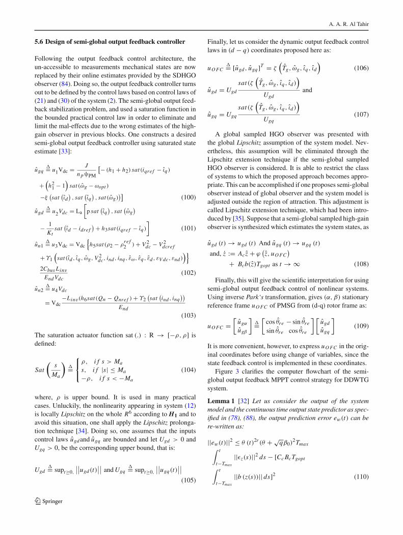
5.6 Design of semi-global output feedback controller

Following the output feedback control architecture, theun-accessible to measurements mechanical states are nowreplaced by their online estimates provided by the SDHGOobserver (84). Doing so, the output feedback controller turnsout to be defined by the control laws based on control laws of(21) and (30) of the system (2). The semi-global output feed-back stabilization problem, and used a saturation function inthe bounded practical control law in order to eliminate andlimit the mal-effects due to the wrong estimates of the high-gain observer in previous blocks. One constructs a desiredsemi-global output feedback controller using saturated stateestimate [33]:

ugq�= u1Vdc = J

n pψPM

[− (h1 + h2) sat (iqre f − ιq )

+(

h21 − 1)

sat (ωg − ωopt )

−ξ(sat(ιd), sat

(ιq), sat (ωg)

)](100)

ugd�= u2Vdc = La

[p sat

(ιq), sat

(ωg)

− 1

Ktsat(ιd − idre f

)+ h3sat (iqre f − ιq )

](101)

un1�= u3Vdc = Vdc

{h5sat (ρ2 − ρ

re f2 ) + V 2

dc − V 2dcre f

+Υ1

(sat (ιd , ιq , ωg, V 2

dc, ind , inq , εω, εq , εd , εV dc, εnd ))}

2Cbus Linv

End Vdc(102)

un2�= u4Vdc

= Vdc−Linv(h6sat (Qn − Qnre f ) + Υ2

(sat(ind , inq

))End

(103)

The saturation actuator function sat (.) : R → [−ρ, ρ] isdefined:

Sat

(s

Ma

)�=⎧⎨⎩

ρ, i f s > Ma

s, i f |s| ≤ Ma

−ρ, i f s < −Ma

(104)

where, ρ is upper bound. It is used in many practicalcases. Unluckily, the nonlinearity appearing in system (12)is locally Lipschitz on the whole R6 according to H1 and toavoid this situation, one shall apply the Lipschitz prolonga-tion technique [34]. Doing so, one assumes that the inputscontrol laws ugdand ugq are bounded and let Ugd > 0 andUgq > 0, be the corresponding upper bound, that is:

Ugd�= supt≥0,

∣∣∣∣ugd(t)∣∣∣∣ andUgq

�= supt≥0,

∣∣∣∣ugq(t)∣∣∣∣(105)

Finally, let us consider the dynamic output feedback controllaws in (d − q) coordinates proposed here as:

uO FC�= [ugd , ugq ]T = ζ

(Tg, ωg, ιq , ιd

)(106)

ugd = Ugd

sat (ζ(

Tg, ωg, ιq , ιd))

Ugdand

ugq = Ugq

sat (ζ(

Tg, ωg, ιq , ιd))

Ugq(107)

A global sampled HGO observer was presented withthe global Lipschitz assumption of the system model. Nev-ertheless, this assumption will be eliminated through theLipschitz extension technique if the semi-global sampledHGO observer is considered. It is able to restrict the classof systems to which the proposed approach becomes appro-priate. This can be accomplished if one proposes semi-globalobserver instead of global observer and the system model isadjusted outside the region of attraction. This adjustment iscalled Lipschitz extension technique, which had been intro-duced by [35]. Suppose that a semi-global sampled high-gainobserver is synthesized which estimates the system states, as

ugd (t) → ugd (t) And ugq (t) → ugq (t)

and, z := Acz + ϕ(z, uO FC

)+ Bcb(z)Tgopt as t → ∞ (108)

Finally, this will give the scientific interpretation for usingsemi-global output feedback control of nonlinear systems.Using inverse Park‘s transformation, gives (α, β) stationaryreference frame uO FC of PMSG from (d-q) rotor frame as:

uO FC =[

ugα

ugβ

]�=[cos θre − sin θre

sin θre cos θre

] [ugd

ugq

](109)

It is more convenient, however, to express uO FC in the orig-inal coordinates before using change of variables, since thestate feedback control is implemented in these coordinates.

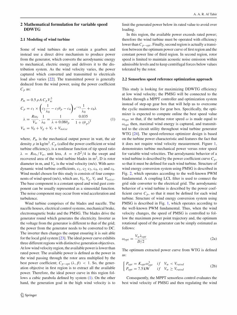
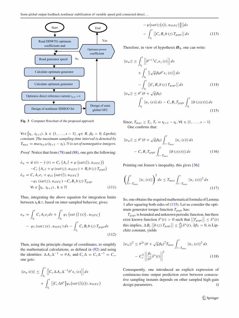
Figure 3 clarifies the computer flowchart of the semi-global output feedback MPPT control strategy for DDWTGsystem.

Lemma 1 [32] Let us consider the output of the systemmodel and the continuous time output state predictor as spec-ified in (78), (88), the output prediction error ew(t) can bere-written as:

||ew(t)||2 ≤ θ (t)2r (θ + √qβ0)

2Tmax∫ t

t−Tmax

||εz(s)||2 ds − [Cc BcTgopt

∫ t

t−Tmax

||b (z(s))|| ds]2 (110)

123

Semi-global output feedback nonlinear stabilization of variable speed grid connected direct. . .

Read DDWTG optimum coefficients and

Read generator speed

Design of nonlinear SDHGO for

Yes

Calculate optimum generator

Design of semi global OFC

Start

Calculate optimum generator

Optimize direct reference current

End

Optimum powercoefficient

No

Fig. 3 Computer flowchart of the proposed approach

∀t∈ [tk, tk+1) , k ∈ {1, . . . , s − 1} , q∈ R, β0 > 0, Lipchitzconstant. The maximum sampling time interval is denoted byTmax = maxk∈N (tk+1 − tk),N is set of nonnegative integers.

Proof Notice that from (78) and (88), one gets the following:

ew = w (t) − y (t) = Cc(

Acz + ϕ(sat (z), uO FC

))−Cc

(Acz + ϕ (sat (z), uO FC ) + Bcb (z) Tgopt

)ew = Cc Acez + ϕo1

(sat (z), uO FC

)−ϕ1 (sat (z), uO FC ) −Cc Bcb (z) Tgopt

∀t ∈ [tk, tk+1) , k ∈ N (111)

Thus, integrating the above equation for integration limitsbetween tk& t , based on inter-sampled behavior, gives:

ew =∫ t

tkCc Acezds +

∫ t

tkϕ1(sat(z (s)

), uO FC

)

− ϕ1 (satz (s) , uO FC ) ds −∫ t

tkCc Bcb (z) Tgopt ds

(112)

Then, using the principle change of coordinates, to simplifythe mathematical calculations, as defined in (92) and usingthe identities: �Ac�

−1 = θ Ac and Cc� = Cc�−1 = Cc,

one gets:

||ew (t)|| ≤∫ t

tk

∣∣∣∣∣∣Cc�Ac�−1θrεz (s)

∣∣∣∣∣∣ ds

+∫ t

tk

∣∣∣∣Cc�θr [ϕo(sat (z

(s)), uO FC

)

−ϕ(sat (z

(s)), uO FC

)]∣∣∣∣ds

−∫ t

tk

∣∣∣∣Cc Bcb (z) Tgopt∣∣∣∣ ds (113)

Therefore, in view of hypothesis H1, one can write:

||ew|| ≤∫ t

tk

∣∣∣∣∣∣θr+1Ccεz (s)∣∣∣∣∣∣ ds

+∫ t

tk

∣∣∣∣√qβ0θrεz (s)

∣∣∣∣ ds

−∫ t

tk

∣∣∣∣Cc Bcb (z) Tgopt∣∣∣∣ ds (114)

||ew|| ≤ θr (θ + √qβ0)∫ t

tk||εz (s)|| ds − Cc BcTgopt

∫ t

tk||b (z(s))|| ds

(115)

Since, Tmax ≥ Ts, Ts = tk+1 − tk,∀k ∈ {1, . . . , s − 1}One confirms that:

||ew|| ≤ θr (θ + √qβ0)

∫ t

t−Tmax

||εz (s)|| ds

− Cc BcTgopt

∫ t

t−Tmax

||b (z(s))|| ds (116)

Pointing out Jensen‘s inequality, this gives [36]:

(∫ t

t−Tmax

||εz (s)||)2

ds ≤ Tmax

∫ t

t−Tmax

||εz (s)||2 ds

(117)

So, one obtains the requiredmathematical formula of Lemma1 after squaring both sides of (115). Let us consider the opti-mum generator torque function Tgopt has:

Tgopt is bounded and unknown periodic function, but thereexist known function δ∗(t) > 0 such that

∣∣∣∣Tgopt∣∣∣∣ ≤ δ∗(t)

this implies, �Bc∣∣∣∣b (z) Tgopt

∣∣∣∣ ≤ β1θ2

δ∗(t), ∃β1 > 0, is Lip-chitz constant, yields

||ew||2 ≤ θ2r (θ + √qβ0)

2Tmax

∫ t

t−Tmax

||εz (s)||2 ds

− C2c

∣∣∣∣∣∣∣∣β1

θ2δ∗(t)

∣∣∣∣∣∣∣∣2

(118)

Consequently, one introduced an explicit expression ofcontinuous-time output prediction error between consecu-tive sampling instants depends on other sampled high-gaindesign parameters. ��

123

A. A. R. Al Tahir

6 Stability analysis of the proposed sampled HGOdesign

Part I: Stability convergence analysisIn order to prepare an upper bound solution of maximum

admissible sampling period and to ensure the semi-globalexponential convergence of the observation error towardszero, this study will re-formulate the theoretical resultsintroduced by [32] in a more convenient and compati-ble for the case study in form of the Lyapunov-basedanalysis,which consists of directLyapunov function andLya-punov Krasovskii functional LKFmethod for time dependentsampled-data systems:

W0 (εz)�= εT

z Pεz + 1

Tmax

∫ t

t−Tmax

∫ t

s||εz ||2 (ξ)dξ ds

(119)

where P is a symmetric positive definite SPD matrix suchthat P = PT ≥ 0, P ∈ R6×6.

For some real constant 0 < σ ≤ 1, σ In ≤ P ≤ In ,therefore, P satisfies the algebraic Lyapunov equation statedin (81). Let us split the proposed overall Lyapunov functioninto two functions named, W1 and W2, such that:

W4 (εz)�= εT

z Pεz (120)

W5 (εz)�= 1

Tmax

∫ t

t−Tmax

∫ t

s||εz(ξ)||2 dξds (121)

The time derivative of the overall Lyapunov functions alongthe closed-loop trajectory of (98) in (118) and (119) is givenby:

W0 (εz) = W4 (εz) + W5 (εz)

One still use, W4 (εz) = εTz P εz + εz

T Pεz (122)

Let us use the variable, t0 ∈ R, within the integrationlimits of (119), one can re-write (119) in new form as:

W5 (εz)�=∫ t

t0||εz (ξ)||2 dξ

− 1

Tmax

∫ t

t−Tmax

∫ s

t0||εz (ξ)||2dξds

So, the time derivative of the fifth Lyapunov functions alongthe closed-loop trajectory of (99) is:

W5 (εz) = ||εz ||2 − 1

Tmax

∫ t

t−Tmax

||εz (s)||2 ds (123)

In view of (98), one can calculate the time derivative of thefourth Lyapunov function along the closed loop trajectory as:

W4 = θεTz

[(Ac − K Cc)

T P]εz

+ 2

θrεT

z P�{ϕo(sat (z), uO FC

)−ϕ (sat (z), uO FC )}

+ 2

θr−1 εTz P K ew − 2

θrPεT

z Bcb (z) Tgopt

−2θ

θεT

z P Dεz (124)

In view of algebraic Lyapunov function stated in (81) tochoose P and the definition of diagonal matrix stated in (79),the time derivative of fourth Lyapunov function in (122):

W4 (εz) ≤ −(

θμ + 2rθ

θ

)I6W1 (εz)

+ 2

θrεT

z P�{ϕo(sat(z), uO FC

)− ϕ (sat (z) , uO FC )}

+ 2

θr−1 εTz P K ew − 2

θrPεT

z Bcb (z) Tgopt − 2θ

θεT

z P Eεz

(125)

Aswell as the strictly positive real number r > 1, is chosensuch that it satisfies the following linear matrix inequality[32]:

− r P ≤ P E + E P ≤ r P (126)

Thus, according to (124), the last term of (123) becomes:

−2θ

θεT

z P Eεz ≤ r

∣∣θ ∣∣θ

εT Pεz (127)

W4 (εz) ≤ −(

θμ + 2rθ

θ− r

∣∣θ ∣∣θ

)W1 (εz)

+ 2

θrεT

z P�{ϕo(sat (z), uO FC

)− ϕ (sat (z), uO FC )}

+ 2

θr−1 εTz P K ew − 2

θrPεT

z Bcb (z) Tgopt (128)

In view of first inductive hypothesisH1 for locally Lipschitzfunction, one deduces that:

W4 (εz) ≤ −[θμ + 2r

θ

θ− r

∣∣θ ∣∣θ

− 2√

qβ0λmax (P)

λmin (P)

]

×W1 (εz)

+ 2

θr−1 εTz P K ew − 2

θrεT

z P Bcb (z) Tgopt (129)

Using the well-known inequality called Young’s inequality,let us choose X = Y = 2 → 1

X + 1Y = 1, that is a2

ϑ+ϑb2 ≥

ab, ∀ϑ > 0, one shall choose, ϑ = μθλmin(P)2 , this implies:

123

Semi-global output feedback nonlinear stabilization of variable speed grid connected direct. . .

W4 (εz) ≤ −[

θ

2μ + 2r

θ

θ− r

∣∣θ ∣∣θ

− 2√

qβ0λmax (P)

λmin (P)

]

W1 (εz) + 2λmax2 (P)

θ2r−2μλmin (P)

||K ||2 ||ew||2 − 2

θrεT

z P�Bcb (z) Tgopt (130)

According to Lemma 1, it leads us to get the followingexpression for Lyapunov equation ∀t∈ [tk, tk+1):

W4(εz) ≤ −[θ

2μ + 2r

θ

θ− r

|θ |θ

− 2√

qβ0λmax(P)

λmin(P)

]

W1(εz) + Tmax θ2r[θ +√qβ0

]2(

2 λ max2(P)

θ2r−1 μλ min(P)||K ||2

∫ t

t−Tmax

||εz (s)||2 ds

− 2

θrεz

T P�Bb(z)Tgopt (131)

Adding the time derivative of Lyapunov functions statedin (122) and (128), respectively, which will give the overalltime derivative ofLyapunov function is: W0 (εz) = W4 (εz)+W5 (εz)

W0 (εz) = −[

θ

2μ + 2r

θ

θ− r

∣∣θ ∣∣θ

− 2√6β0

λmax (P)

λmin (P)

]W1 (εz)

+Tmax [θ + √6β0])2 2θλmax2 (P)

μλmin (P)||K ||2

∫ t

t−Tmax

||εz (s)||2 ds − + 2

θrεT

z P�Bcb (z) Tgopt

−C2c

∣∣∣∣∣∣∣∣β1

θ2δ

∣∣∣∣∣∣∣∣2

+[||εz ||2 − + 1

Tmax

∫ t

t−Tmax∫ t

s||εz (s)||2 ds

](132)

Part II: Derivative of maximum allowable samplingperiod

Let us bound the parameter q = 6, for the sample studyof sixth order state-space representation.

W0 (εz) ≤−[

θ

2μ+2r

θ

θ t− r

∣∣θ ∣∣θ t

− 2√6β0

λmax (P)

λmin (P)

]

W1 (εz) −[

1

Tmax−T max

2θλmax2 (P)

μλmin (P)||K ||2

(θ + √

6 β0

)]2∫ t

t−Tmax

||εz (s)||2 ds − 2

θrεT

z P�Bcb (z) Tgopt

−C2c

∣∣∣∣∣∣∣∣β1

θ2δ

∣∣∣∣∣∣∣∣2

(133)

To create semi-global exponential convergence of the obser-vation error under output feedback nonlinear control andto ensure that the time derivative of the overall Lyapunov

function given in (130) is negative, this study will introducean explicit expression for upper bound of sampling intervaldepends on other design parameters as follows:

[1

Tmax− Tmax

2θλmax2 (P)

μλmin (P)||K ||2

(θ + √

6β0

)2] ≥ 0

Finally, taking root mean square for both sides, q = 6, andθ → θmax , thus, ∀θmax ≥ θ (t0) > 1, and ∀Ts ∈ (0, Tmax ] ispiecewise function, yields:

Tmax ≤√

μλmin (P)√2θmaxλmax (P) ||K || (θmax + √

6β0(134)

where, θmax is the maximum amplitude of the high gaindesign parameter, ∀t ∈ R+, β0 > 0 and λmin (P), λmax (P)

are respectively the largest and smallest eigenvalues of thepositive definite matrix P. Using the following property:

λmin (P) ||εz (s)||2 ≤ W1 (εz) ≤ λmax (P) ||εz ||2, andone shall get after substituting (131) in (130),

W0 (εz) ≤ −[

θ

2μ + 2r

θ

θ− r

∣∣θ ∣∣θ

− 2√6β0

λmax (P) + 1

λmin (P)

]

W1 (εz) − + 2

θrεT

z P�Bcb (z) Tgopt − C2c

∣∣∣∣∣∣∣∣β1

θ2δ∗(t)

∣∣∣∣∣∣∣∣2

(135)

As the dynamic HGO design parameter is increasing in thediscrete time interval

[tk , tk+1), let us select the dynamic

high-gain observer design parameter θ or g (θ) , g : R → Rfunction describing the observer design parameter with theadaptation process is driven by assessment of the systemmodel nonlinearities that will guarantee to enlarge the sam-pling period with fast convergence:

θ�= −θ

r

[μ

2θ + 2r

θ + ∣∣θ ∣∣β0λmax (P)

θ λmin (P)

](136)

The adaptation is driven by assessment of the system modelnonlinearities.

To summarize the proposed main theorem, using Lya-punov stability approach of nonlinear systems, one concludesthat, with the choice for the gain matrix corresponding tomeasurements error K stated in (80) and it submitted toalgebraic Lyapunov equation in (81), the DHGOdesign para-meter θ = g (θ) proposed in (133) and explicitly introduce anupper bound of positive sampling period Tmax stated in (131)supported by semi-global sampled HGO observer defined in(84), ∀t ∈ [tk, tk+1) , k ∈ N, as well as introduce an explicitexpression for output prediction error for time dependentof sampled systems in terms of other design parameters forwhatever initial state variables stated in (116) and confirming

123

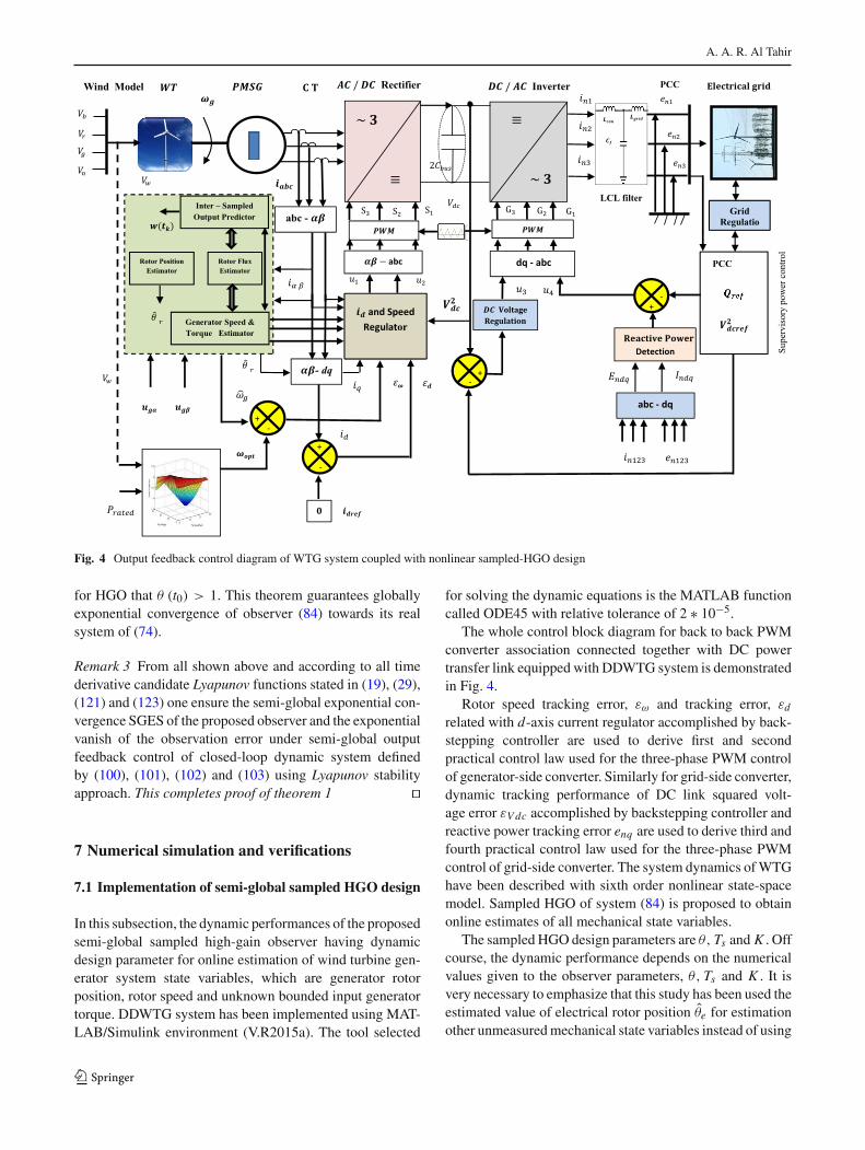
A. A. R. Al Tahir

Fig. 4 Output feedback control diagram of WTG system coupled with nonlinear sampled-HGO design

for HGO that θ (t0) > 1. This theorem guarantees globallyexponential convergence of observer (84) towards its realsystem of (74).

Remark 3 From all shown above and according to all timederivative candidate Lyapunov functions stated in (19), (29),(121) and (123) one ensure the semi-global exponential con-vergence SGES of the proposed observer and the exponentialvanish of the observation error under semi-global outputfeedback control of closed-loop dynamic system definedby (100), (101), (102) and (103) using Lyapunov stabilityapproach. This completes proof of theorem 1 ��

7 Numerical simulation and verifications

7.1 Implementation of semi-global sampled HGO design

In this subsection, the dynamic performances of the proposedsemi-global sampled high-gain observer having dynamicdesign parameter for online estimation of wind turbine gen-erator system state variables, which are generator rotorposition, rotor speed and unknown bounded input generatortorque. DDWTG system has been implemented using MAT-LAB/Simulink environment (V.R2015a). The tool selected

for solving the dynamic equations is the MATLAB functioncalled ODE45 with relative tolerance of 2 ∗ 10−5.

The whole control block diagram for back to back PWMconverter association connected together with DC powertransfer link equipped with DDWTG system is demonstratedin Fig. 4.

Rotor speed tracking error, εω and tracking error, εd

related with d-axis current regulator accomplished by back-stepping controller are used to derive first and secondpractical control law used for the three-phase PWM controlof generator-side converter. Similarly for grid-side converter,dynamic tracking performance of DC link squared volt-age error εV dc accomplished by backstepping controller andreactive power tracking error enq are used to derive third andfourth practical control law used for the three-phase PWMcontrol of grid-side converter. The system dynamics ofWTGhave been described with sixth order nonlinear state-spacemodel. Sampled HGO of system (84) is proposed to obtainonline estimates of all mechanical state variables.

The sampled HGO design parameters are θ, Ts and K . Offcourse, the dynamic performance depends on the numericalvalues given to the observer parameters, θ, Ts and K . It isvery necessary to emphasize that this study has been used theestimated value of electrical rotor position θe for estimationother unmeasuredmechanical state variables instead of using

123

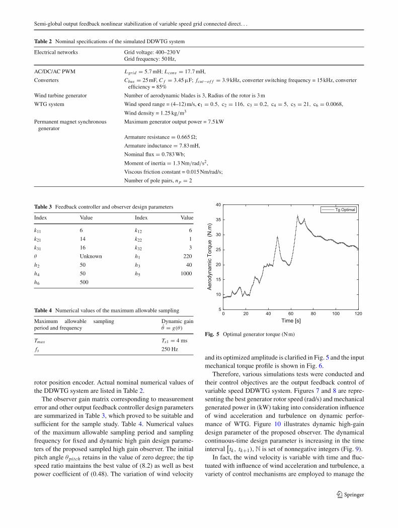
Semi-global output feedback nonlinear stabilization of variable speed grid connected direct. . .

Table 2 Nominal specifications of the simulated DDWTG system

Electrical networks Grid voltage: 400–230VGrid frequency: 50Hz,

AC/DC/AC PWM Lgrid = 5.7mH; Lconv = 17.7mH,

Converters Cbus = 25mF, C f = 3.45μF; fcut−of f = 3.9kHz, converter switching frequency = 15kHz, converterefficiency = 85%

Wind turbine generator Number of aerodynamic blades is 3, Radius of the rotor is 3m

WTG system Wind speed range = (4–12)m/s, c1 = 0.5, c2 = 116, c3 = 0.2, c4 = 5, c5 = 21, c6 = 0.0068,

Wind density = 1.25 kg/m3

Permanent magnet synchronousgenerator

Maximum generator output power = 7.5kW

Armature resistance = 0.665�;

Armature inductance = 7.83mH,

Nominal flux = 0.783Wb;

Moment of inertia = 1.3Nm/rad/s2,

Viscous friction constant = 0.015Nm/rad/s;

Number of pole pairs, n p = 2

Table 3 Feedback controller and observer design parameters

Index Value Index Value

k11 6 k12 6

k21 14 k22 1

k31 16 k32 3

θ Unknown h1 220

h2 50 h3 40

h4 50 h5 1000

h6 500

Table 4 Numerical values of the maximum allowable sampling

Maximum allowable samplingperiod and frequency

Dynamic gainθ = g(θ)

Tmax Ts1 = 4 ms

fs 250 Hz

rotor position encoder. Actual nominal numerical values ofthe DDWTG system are listed in Table 2.

The observer gain matrix corresponding to measurementerror and other output feedback controller design parametersare summarized in Table 3, which proved to be suitable andsufficient for the sample study. Table 4. Numerical valuesof the maximum allowable sampling period and samplingfrequency for fixed and dynamic high gain design parame-ters of the proposed sampled high gain observer. The initialpitch angle θpitch retains in the value of zero degree; the tipspeed ratio maintains the best value of (8.2) as well as bestpower coefficient of (0.48). The variation of wind velocity

Time [s]0 20 40 60 80 100 120

Aer

odyn

amic

Tor

que

(N.m

)

5

10

15

20

25

30

35

40Tg Optimal

Fig. 5 Optimal generator torque (Nm)

and its optimized amplitude is clarified in Fig. 5 and the inputmechanical torque profile is shown in Fig. 6.

Therefore, various simulations tests were conducted andtheir control objectives are the output feedback control ofvariable speed DDWTG system. Figures 7 and 8 are repre-senting the best generator rotor speed (rad/s) and mechanicalgenerated power in (kW) taking into consideration influenceof wind acceleration and turbulence on dynamic perfor-mance of WTG. Figure 10 illustrates dynamic high-gaindesign parameter of the proposed observer. The dynamicalcontinuous-time design parameter is increasing in the timeinterval

[tk, tk+1), N is set of nonnegative integers (Fig. 9).

In fact, the wind velocity is variable with time and fluc-tuated with influence of wind acceleration and turbulence, avariety of control mechanisms are employed to manage the

123

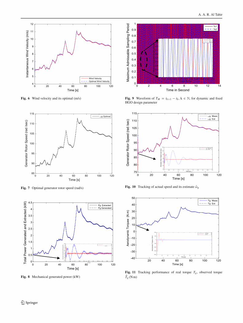
A. A. R. Al Tahir

Time [s]0 20 40 60 80 100 120

Inst

anta

neou

s W

ind

Velo

city

(m/s

)

4

5

6

7

8

9

10

11

12

Fig. 6 Wind velocity and its optimal (m/s)

Time [s]0 20 40 60 80 100 120

Gen

erat

or R

otor

Spe

ed (r

ad /s

ec)

85

90

95

100

105

110

115

Fig. 7 Optimal generator rotor speed (rad/s)

Time [s]

Time [s]

0 20 40 60 80 100 120Tota

l Pow

er G

ener

ated

and

Ext

ract

ed (k

W)

0

0.5

1

1.5

2

2.5

3

3.5

4

4.5

0 0.05 0.1 0.15 0.2 0.25 0.3 0.35 0.4 0.45 0.5

Tota

l Pow

er G

ener

ated

and

Ext

ract

ed (k

W)

0.35

0.4

0.45

0.5

0.55

0.6

0.65

0.7

0.75

0.8

0.85

Pg Extracted

Pg Generated

Pg ExtractedPg Generated

Fig. 8 Mechanical generated power (kW)

Time in Second0 2 4 6 8 10 12 14

Max

imum

Adm

issa

ble

Sam

plin

g P

erio

d

0

0.1

0.2

0.3

0.4

0.5

0.6

0.7

0.8

0.9

1

Fig. 9 Waveform of TM = tk+1 − tk , k ∈ N, for dynamic and fixedHGO design parameter

Time [s]

Time [s]

0 20 40 60 80 100 120

Gen

erat

or R

otor

Spe

ed (r

ad /s

ec)

75

80

85

90

95

100

105

110

115

0 0.05 0.1 0.15 0.2 0.25 0.3 0.35 0.4 0.45 0.5

Gen

erat

or R

otor

Spe

ed (r

ad /s

ec)

75

80

85

90

95

100

105

Fig. 10 Tracking of actual speed and its estimate ωg

Time [s]20 40 60 80 100 120

Aero

dyna

mic

Tor

quee

(N

.m)

-40

-30

-20

-10

0

10

20

30

40

50

Time [s]0 0.1 0.2 0.3 0.4 0.5 0.6 0.7 0.8 0.9 1

Aer

odyn

amic

Tor

quee

(N

.m)

-2000

-1500

-1000

-500

0

500

1000Tg MeasTg Est

Fig. 11 Tracking performance of real torque Tg , observed torqueTg (Nm)

123

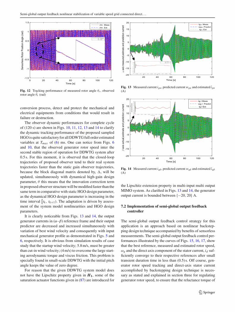
Semi-global output feedback nonlinear stabilization of variable speed grid connected direct. . .

Fig. 12 Tracking performance of measured rotor angle θr , observedrotor angle θr (rad)

conversion process, detect and protect the mechanical andelectrical equipments from conditions that would result infailure or destruction.

The observer dynamic performances for complete cycleof (120 s) are shown in Figs. 10, 11, 12, 13 and 14 to clarifythe dynamic tracking performance of the proposed sampledHGOis quite satisfactory for allDDWTGfull order estimatedvariables at Tmax of (6) ms. One can notice from Figs. 6and 10, that the observed generator rotor speed inter thesecond stable region of operation for DDWTG system after0.5 s. For this moment, it is observed that the closed-looptrajectories of proposed observer tend to their real systemtrajectories faster than the static gain observer trajectories,because the block diagonal matrix denoted by, �, will beupdated, simultaneously with dynamical high-gain designparameter, θ this means that the innovation correction termin proposed observer structurewill bemodified faster than thesame term in comparative with static HGO design parameter,as the dynamical HGO design parameter is increasing in thetime interval

[tk, tk+1). The adaptation is driven by assess-

ment of the system model nonlinearities and HGO designparameters.

It is clearly noticeable from Figs. 13 and 14, the outputgenerator currents in (α–β) reference frame and their outputpredictor are decreased and increased simultaneously withvariation of best wind velocity and consequently with inputmechanical generator profile as demonstrated in Figs. 5 and6, respectively. It is obvious from simulation results of casestudy that the startup wind velocity; 5.8m/s, must be greaterthan cut-in wind velocity; (4m/s) to overcome the large start-ing aerodynamic torque and viscus friction. This problem isspecially found in small-scale DDWTGwith the initial pitchangle keeps the value of zero degree.

For reason that the given DDWTG system model doesnot have the Lipschitz property given in H1, some of thesaturation actuator functions given in (87) are introduced for

Fig. 13 Measured current igα , predicted currentwgα and estimated ιgα

(A)

Fig. 14 Measured current igβ , predicted currentwgβ and estimated ιgβ(A)

the Lipschitz extension property in multi-input multi outputMIMO system. As clarified in Figs. 13 and 14, the generatoroutput current is bounded between {−20, 20} A.

7.2 Implementation of semi-global output feedbackcontroller

The semi-global output feedback control strategy for thisapplication is an approach based on nonlinear backstep-ping design technique accompanied by benefits of sensorlessmeasurements. The semi-global output feedback control per-formances illustrated by the curves of Figs. 15, 16, 17, showthat the best reference, measured and estimated rotor speed,ωg and the direct axis component of the stator current, id suf-ficiently converge to their respective references after smalltransient duration time in less than (0.5) s. Off course, gen-erator rotor speed tracking and direct-axis stator currentaccomplished by backstepping design technique is neces-sary as stated and explained in section three for regulatinggenerator rotor speed, to ensure that the reluctance torque of

123

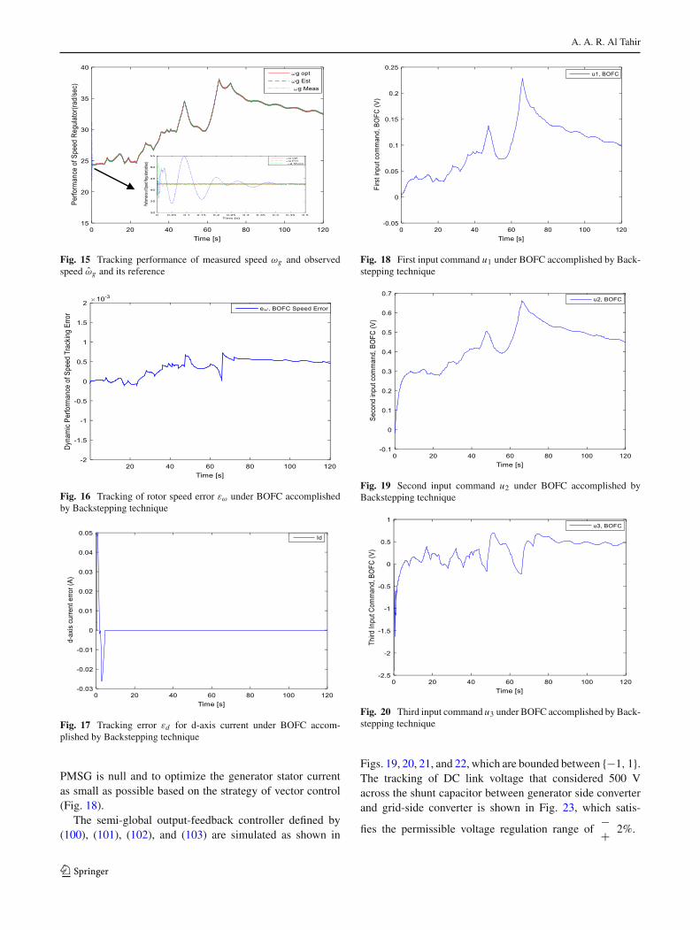
A. A. R. Al Tahir

Fig. 15 Tracking performance of measured speed ωg and observedspeed ωg and its reference

Fig. 16 Tracking of rotor speed error εω under BOFC accomplishedby Backstepping technique

Fig. 17 Tracking error εd for d-axis current under BOFC accom-plished by Backstepping technique

PMSG is null and to optimize the generator stator currentas small as possible based on the strategy of vector control(Fig. 18).

The semi-global output-feedback controller defined by(100), (101), (102), and (103) are simulated as shown in

Fig. 18 First input command u1 under BOFC accomplished by Back-stepping technique

Fig. 19 Second input command u2 under BOFC accomplished byBackstepping technique

Fig. 20 Third input command u3 under BOFC accomplished by Back-stepping technique

Figs. 19, 20, 21, and 22, which are bounded between {−1, 1}.The tracking of DC link voltage that considered 500 Vacross the shunt capacitor between generator side converterand grid-side converter is shown in Fig. 23, which satis-

fies the permissible voltage regulation range of−+ 2%.

123

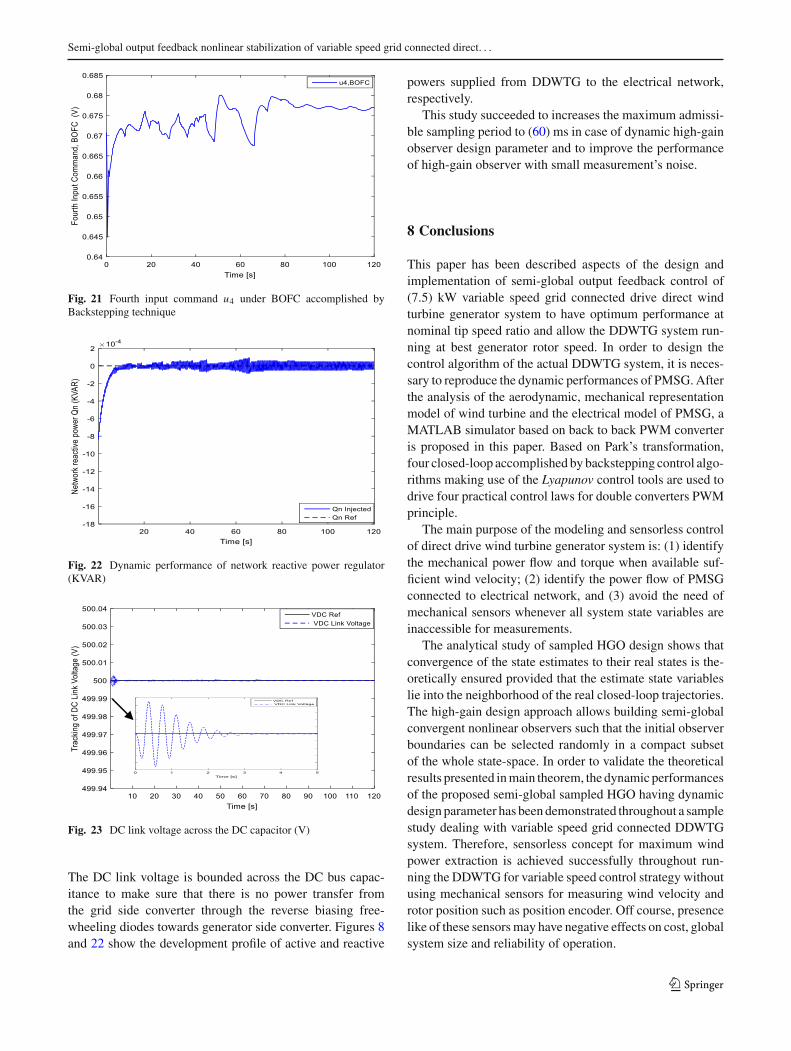
Semi-global output feedback nonlinear stabilization of variable speed grid connected direct. . .

Fig. 21 Fourth input command u4 under BOFC accomplished byBackstepping technique

Fig. 22 Dynamic performance of network reactive power regulator(KVAR)

Fig. 23 DC link voltage across the DC capacitor (V)

The DC link voltage is bounded across the DC bus capac-itance to make sure that there is no power transfer fromthe grid side converter through the reverse biasing free-wheeling diodes towards generator side converter. Figures 8and 22 show the development profile of active and reactive

powers supplied from DDWTG to the electrical network,respectively.

This study succeeded to increases the maximum admissi-ble sampling period to (60) ms in case of dynamic high-gainobserver design parameter and to improve the performanceof high-gain observer with small measurement’s noise.

8 Conclusions

This paper has been described aspects of the design andimplementation of semi-global output feedback control of(7.5) kW variable speed grid connected drive direct windturbine generator system to have optimum performance atnominal tip speed ratio and allow the DDWTG system run-ning at best generator rotor speed. In order to design thecontrol algorithm of the actual DDWTG system, it is neces-sary to reproduce the dynamic performances of PMSG. Afterthe analysis of the aerodynamic, mechanical representationmodel of wind turbine and the electrical model of PMSG, aMATLAB simulator based on back to back PWM converteris proposed in this paper. Based on Park’s transformation,four closed-loop accomplished by backstepping control algo-rithms making use of the Lyapunov control tools are used todrive four practical control laws for double converters PWMprinciple.

The main purpose of the modeling and sensorless controlof direct drive wind turbine generator system is: (1) identifythe mechanical power flow and torque when available suf-ficient wind velocity; (2) identify the power flow of PMSGconnected to electrical network, and (3) avoid the need ofmechanical sensors whenever all system state variables areinaccessible for measurements.

The analytical study of sampled HGO design shows thatconvergence of the state estimates to their real states is the-oretically ensured provided that the estimate state variableslie into the neighborhood of the real closed-loop trajectories.The high-gain design approach allows building semi-globalconvergent nonlinear observers such that the initial observerboundaries can be selected randomly in a compact subsetof the whole state-space. In order to validate the theoreticalresults presented inmain theorem, the dynamic performancesof the proposed semi-global sampled HGO having dynamicdesign parameter has beendemonstrated throughout a samplestudy dealing with variable speed grid connected DDWTGsystem. Therefore, sensorless concept for maximum windpower extraction is achieved successfully throughout run-ning the DDWTG for variable speed control strategy withoutusing mechanical sensors for measuring wind velocity androtor position such as position encoder. Off course, presencelike of these sensorsmay have negative effects on cost, globalsystem size and reliability of operation.

123

A. A. R. Al Tahir

The Lyapunov Krasovskii candidate functional LKFapproach makes possible the design of semi-global outputfeedback control considering different specifications dealingwith stability and stabilization of sampled control systemswith applications concerning with several sciences and prac-tical engineering applications.

On other hand, state-feedback control may cause degra-dation or deterioration of the control performance, expensivecontrol and unreliable behaviors. Consequently, semi-globaloutput feedback process is very important for the reason thatin the practical engineering applications, some of the statevariables cannot be measured directly throughout measure-ment devices such as generator rotor speed and rotor positionangle.

The simulation results of the demonstrated sample studyhave been shown that the proposed sampled HGO hasfast transient response, which makes control task easier,good input generator mechanical torque rejection due to thedisturbing effect and wind turbulence, accurate power track-ing response, robustness of observer performance, smoothmotion at low generator speed and efficient operation at highrotor angular speed. The simulation results supported thepresented main theory and the improvement with respect tosemi-global convergence properties and system state esti-mates.

Furthermore, the analysis of the control structure is devel-oped depending on the advanced chosen power electronicconverters such as buck to buck PWM converter. The speedcontrol scheme for DDWTG system has been presented andsimulated, showing that this approach offers an excellent per-formance to place the PMSG at the desired speed regulation.The active power is generated using DC bus voltage regula-tor and the reactive power is set as the requirements of theelectrical grid, and omitted if a unity power factor correctionis the demanded.

Acknowledgements This work is partially supported by the ministryof higher education and scientific research in Iraq to carry out thisresearch with original results.

Open Access This article is distributed under the terms of the CreativeCommons Attribution 4.0 International License (http://creativecommons.org/licenses/by/4.0/), which permits unrestricted use, distribution,and reproduction in any medium, provided you give appropriate creditto the original author(s) and the source, provide a link to the CreativeCommons license, and indicate if changes were made.

References

1. Executive Office of the President (2013) The president’s climateaction plan. White house washington. www.whitehouse.gov

2. Jia Y, Wang Q, Yang Z (2007) Experimental study of control strat-egy for wind generation system. IEEE power electronics specialistconference, PESC, pp 1202–1207

3. Dehghan M, Mohamadian M, Varjani AY (2009) A new variable-speed wind energy conversion system using permanent-magnetsynchronous generator and z-source inverter. IEEE Trans EnergyConvers 24(3):714–724

4. Errami Y, Ouassaid M, Maaroufi M (2011) Modelling and controlstrategy of PMSG based variable speed wind energy conversionsystem. International conference on multimedia computing andsystems—ICMCS, Ouarzazate, pp 1–6

5. Babu N, Arulmozhivarman P (2013) Wind energy conversionsystems—a technical review. J Eng Sci Technol 8(4):493–507

6. Shim H, Seo JH (2000) Recursive observer design beyond the uni-form observability. In: Proceedings of the 39th IEEE conferenceon decision and control, vol 1, pp 809–814

7. Gauthier J, Kupka I (2001) Deterministic observation theory andapplications. Cambridge University Press, Cambridge. ISBN 0521805937

8. Andrieu V, Parly L, Astolfi A (2009) High-gain observers withupdated gain and homogeneous correction terms. Automatica45(2):422–428

9. Ahrens J, Khalil HK (2009) High-gain observers in the pres-ence of measurement noise: a switched-gain approach. Automatica45:936–943

10. Boizot N, Busvelle E, Gauthier JP (2010) An adaptive high gainobserver for nonlinear systems. Automatica 46(9):1483–1488

11. Beltran B, Ahmed-Ali T, Benbouzid ME (2007) Sliding modepower control of variable speed wind energy conversion systems.IEEE Trans Energy Convers 23(2):943–948

12. Barambones O (2012) Sliding mode control strategy for wind tur-bine power maximization. J Energ 5(7):2330–2330

13. Loucif M, Boumedine A, Mechernene A (2014) Maximum powerpoint tracking based on backstepping control of wind turbine. Elec-tromicanica Electromachanica Autom 62(3):103–109

14. HusseinM, Senjyu T, Orabi M,WahabM, HamadaM (2013) Con-trol of a stand-alone variable speed wind energy supply system.Appl Sci 3(2):437–456

15. Senjyu T, Ochi Y, Kikunaga Y, Tokudome M, Yona A, MuhandoB, Urasaki N, Funabashi T (2009) Sensorless maximum powerpoint tracking control for wind generation system with squirrelcage induction generator. Renew Energy 34(4):994–999

16. Rocha R (2011) A sensorless control for a variable speed windturbine operating at partial load. Renew Energy 36(1):132–141

17. Fu D, Xing Y, Mas Y (2010) MPPT of VSCF wind energyconversion systemusingxtremumcontrol strategy.Worldnon-grid-connected wind power and energy conference (WNWEC), IEEEconference, pp 1–6

18. Kesraoui M, Korichi N, Belkadi A (2011) Maximum power pointtracker of wind energy conversion system. Renew Energy GenerAppl 36(10):2655–2662

19. Khalil H, Laurent P (2014) High-gain observers in nonlinear feed-back control. Int J Robust Nonlinear Control 24(6):993–1015

20. Dabroom AM, Khalil HK (2001) Output feedback sampled-datacontrol of nonlinear systems using high-gain observers. IEEETransAutomat Control 46:1712–1725

21. Liu M, Liu Y, Li F (2015) Semi-global stabilization via output-feedback for a class of non-triangular nonlinear systems with anunknown coefficient. Hindawi Publishing Corporation Mathemat-ical Problems in Engineering, pp 3–8

22. Burton T, Jenkins N, Sharpe D, Bossanyi E (2011) Wind energyhandbook, 2nd edn. Wiley, New York

23. Bianchi D, Battista H, Mantz R (2007) Wind turbine control sys-tems: principles, modelling and gain scheduling design. Springer,London

24. ElMagri A, Giri F, Abouloifa A, El Fadili A (2009) Nonlinear con-trol of associations including wind turbine PMSG and AC/DC/ACconverter—speed regulation and power factor correction. IEEEEuropean control conference, pp 23–26

123

Semi-global output feedback nonlinear stabilization of variable speed grid connected direct. . .

25. Moreno JS, BesanconG,Martinez J (2013) Observer—basedmax-imum power tracking in wind turbines with only generator speedmeasurements. European control conference, Switzerland, pp 478–483

26. El Magri A, Giri F, Abouloifa A, Fatima Z (2009) Nonlinear con-trol of associations including synchronous motors and AC/DC/ACconverters: a formal analysis of speed regulation and power factorcorrection. IEEE, American control conference, pp 3470–3475

27. Boumédiène A, Boucherit M, Boudjema F (2007) A robustnesscomparative study of several types of speed controllers with thekind based on backstepping for pmsm control fed by a three-levelvoltage source inverter. Int Rev Electr Eng 2(4):619–633

28. Rashid H (2011) Power electronics handbook: devices, circuits,and applications, 3rd edn. Elsevier Inc, New York. ISBN-10:0123820367

29. Krstic M, Kanellakopoulos I, Kokotovic PV (1995) Nonlinear andadaptive control design. Wiley, New York

30. Koutroulis E (2006) Design of a maximum power tracking sys-tem for wind-energy conversion applications. IEEE Trans IndustrElectron 53(2):486–494

31. El Magri A, Giri F, El fadili A (2013) AC electric motors control:advanced design techniques. Wiley, Oxford. ISBN: 978-1-118-33152-1

32. Hann C (2014) Contribution to the synthesis of observers fornonlinear systems under communication constrains. Ph.D. thesis,UCBN, France

33. Shim H, Seo JH (2000) Nonlinear output feedback stabilization ona bounded region of attraction. Int J Control 73(5):416–426

34. ShimH,TeelAR (2001)Onperformance improvement of an outputfeedback control for non-uniformly observable nonlinear systems.In: Proceeding of the 40’th IEEE conference on decision and con-trol, Orlando, USAP, pp 1354–1359

35. Shim H, Young I, Seo JH (2001) Semi-global observer for multi-output nonlinear systems. Syst Control Lett 42(2001):233–244

36. Fridman E (2014) Introduction to time-delay systems: analysis andcontrol. Birkhauser, Basel. ISBN 9783319093932

123