Semi-Dense Visual Odometry for a Monocular Camera∗

Jakob Engel, Jurgen Sturm, Daniel CremersTU Munchen, Germany

Abstract

We propose a fundamentally novel approach to real-timevisual odometry for a monocular camera. It allows to ben-efit from the simplicity and accuracy of dense tracking –which does not depend on visual features – while runningin real-time on a CPU. The key idea is to continuously esti-mate a semi-dense inverse depth map for the current frame,which in turn is used to track the motion of the camera usingdense image alignment. More specifically, we estimate thedepth of all pixels which have a non-negligible image gradi-ent. Each estimate is represented as a Gaussian probabilitydistribution over the inverse depth. We propagate this in-formation over time, and update it with new measurementsas new images arrive. In terms of tracking accuracy andcomputational speed, the proposed method compares favor-ably to both state-of-the-art dense and feature-based visualodometry and SLAM algorithms. As our method runs inreal-time on a CPU, it is of large practical value for roboticsand augmented reality applications.

1. Towards Dense Monocular Visual OdometryTracking a hand-held camera and recovering the three-

dimensional structure of the environment in real-time isamong the most prominent challenges in computer vision.In the last years, dense approaches to these challenges havebecome increasingly popular: Instead of operating solelyon visual feature positions, they reconstruct and track onthe whole image using a surface-based map and therebyare fundamentally different from feature-based approaches.Yet, these methods are to date either not real-time capableon standard CPUs [11, 15, 17] or require direct depth mea-surements from the sensor [7], making them unsuitable formany practical applications.

In this paper, we propose a novel semi-dense visualodometry approach for a monocular camera, which com-bines the accuracy and robustness of dense approacheswith the efficiency of feature-based methods. Further, itcomputes highly accurate semi-dense depth maps from themonocular images, providing rich information about the 3D

∗ This work was supported by the ERC Starting Grant ConvexVisionand the DFG project Mapping on Demand

far

closeFigure 1. Semi-Dense Monocular Visual Odometry: Our ap-proach works on a semi-dense inverse depth map and combines theaccuracy and robustness of dense visual SLAM methods with theefficiency of feature-based techniques. Left: video frame, Right:color-coded semi-dense depth map, which consists of depth esti-mates in all image regions with sufficient structure.

structure of the environment. We use the term visual odom-etry as supposed to SLAM, as – for simplicity – we deliber-ately maintain only information about the currently visiblescene, instead of building a global world-model.

1.1. Related Work

Feature-based monocular SLAM. In all feature-basedmethods (such as [4, 8]), tracking and mapping consists oftwo separate steps: First, discrete feature observations (i.e.,their locations in the image) are extracted and matched toeach other. Second, the camera and the full feature posesare calculated from a set of such observations – disregard-ing the images themselves. While this preliminary abstrac-tion step greatly reduces the complexity of the overall prob-lem and allows it to be tackled in real time, it inherentlycomes with two significant drawbacks: First, only imageinformation conforming to the respective feature type andparametrization – typically image corners and blobs [6] orline segments [9] – is utilized. Second, features have tobe matched to each other, which often requires the costlycomputation of scale- and rotation-invariant descriptors androbust outlier estimation methods like RANSAC.

Dense monocular SLAM. To overcome these limitationsand to better exploit the available image information, densemonocular SLAM methods [11, 17] have recently been pro-posed. The fundamental difference to keypoint-based ap-proaches is that these methods directly work on the images

1

instead of a set of extracted features, for both mapping andtracking: The world is modeled as dense surface while inturn new frames are tracked using whole-image alignment.This concept removes the need for discrete features, andallows to exploit all information present in the image, in-creasing tracking accuracy and robustness. To date how-ever, doing this in real-time is only possible using modern,powerful GPU processors.

Similar methods are broadly used in combination withRGB-D cameras [7], which directly measure the depth ofeach pixel, or stereo camera rigs [3] – greatly reducing thecomplexity of the problem.

Dense multi-view stereo. Significant prior work exists onmulti-view dense reconstruction, both in a real-time setting[13, 11, 15], as well as off-line [5, 14]. In particular for off-line reconstruction, there is a long history of using differentbaselines to steer the stereo-inherent trade-off between ac-curacy and precision [12]. Most similar to our approach isthe early work of Matthies et al., who proposed probabilis-tic depth map fusion and propagation for image sequences[10], however only for structure from motion, i.e., not cou-pled with subsequent dense tracking.

1.2. Contributions

In this paper, we propose a novel semi-dense approach tomonocular visual odometry, which does not require featurepoints. The key concepts are

• a probabilistic depth map representation,

• tracking based on whole-image alignment,

• the reduction on image-regions which carry informa-tion (semi-dense), and

• the full incorporation of stereo measurement uncer-tainty.

To the best of our knowledge, this is the first featureless,real-time monocular visual odometry approach, which runsin real-time on a CPU.

1.3. Method Outline

Our approach is partially motivated by the basic princi-ple that for most real-time applications, video informationis abundant and cheap to come by. Therefore, the computa-tional budget should be spent such that the expected infor-mation gain is maximized. Instead of reducing the imagesto a sparse set of feature observations however, our methodcontinuously estimates a semi-dense inverse depth map forthe current frame, i.e., a dense depth map covering all imageregions with non-negligible gradient (see Fig. 2). It is com-prised of one inverse depth hypothesis per pixel modeledby a Gaussian probability distribution. This representationstill allows to use whole-image alignment [7] to track new

far

closeoriginal image semi-dense depth map (ours)

keypoint depth map [8] dense depth map [11] RGB-D camera [16]

Figure 2. Semi-Dense Approach: Our approach reconstructs andtracks on a semi-dense inverse depth map, which is dense in allimage regions carrying information (top-right). For comparison,the bottom row shows the respective result from a keypoint-basedapproach, a fully dense approach and the ground truth from anRGB-D camera.

frames, while at the same time greatly reducing computa-tional complexity compared to volumetric methods. Theestimated depth map is propagated from frame to frame,and updated with variable-baseline stereo comparisons. Weexplicitly use prior knowledge about a pixel’s depth to se-lect a suitable reference frame on a per-pixel basis, and tolimit the disparity search range.

The remainder of this paper is organized as follows: Sec-tion 2 describes the semi-dense mapping part of the pro-posed method, including the derivation of the observationaccuracy as well as the probabilistic data fusion, propaga-tion and regularization steps. Section 3 describes how newframes are tracked using whole-image alignment, and Sec. 4summarizes the complete visual odometry method. A qual-itative as well as a quantitative evaluation is presented inSec. 5. We then give a brief conclusion in Sec. 6.

2. Semi-Dense Depth Map EstimationOne of the key ideas proposed in this paper is to esti-

mate a semi-dense inverse depth map for the current cam-era image, which in turn can be used for estimating thecamera pose of the next frame. This depth map is continu-ously propagated from frame to frame, and refined with newstereo depth measurements, which are obtained by perform-ing per-pixel, adaptive-baseline stereo comparisons. Thisallows us to accurately estimate the depth both of close-byand far-away image regions. In contrast to previous workthat accumulates the photometric cost over a sequence ofseveral frames [11, 15], we keep exactly one inverse depthhypothesis per pixel that we represent as Gaussian proba-bility distribution.

This section is comprised of three main parts: Sec-

reference small baseline medium baseline large baseline

0 0.05 0.1 0.15 0.2 0.25 0.30

1

2

smallmediumlarge

cost

inverse depth d

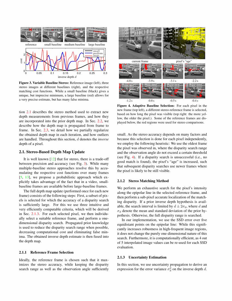
Figure 3. Variable Baseline Stereo: Reference image (left), threestereo images at different baselines (right), and the respectivematching cost functions. While a small baseline (black) gives aunique, but imprecise minimum, a large baseline (red) allows fora very precise estimate, but has many false minima.

tion 2.1 describes the stereo method used to extract newdepth measurements from previous frames, and how theyare incorporated into the prior depth map. In Sec. 2.2, wedescribe how the depth map is propagated from frame toframe. In Sec. 2.3, we detail how we partially regularizethe obtained depth map in each iteration, and how outliersare handled. Throughout this section, d denotes the inversedepth of a pixel.

2.1. Stereo-Based Depth Map Update

It is well known [12] that for stereo, there is a trade-offbetween precision and accuracy (see Fig. 3). While manymultiple-baseline stereo approaches resolve this by accu-mulating the respective cost functions over many frames[5, 13], we propose a probabilistic approach which ex-plicitly takes advantage of the fact that in a video, small-baseline frames are available before large-baseline frames.

The full depth map update (performed once for each newframe) consists of the following steps: First, a subset of pix-els is selected for which the accuracy of a disparity searchis sufficiently large. For this we use three intuitive andvery efficiently computable criteria, which will be derivedin Sec. 2.1.3. For each selected pixel, we then individu-ally select a suitable reference frame, and perform a one-dimensional disparity search. Propagated prior knowledgeis used to reduce the disparity search range when possible,decreasing computational cost and eliminating false min-ima. The obtained inverse depth estimate is then fused intothe depth map.

2.1.1 Reference Frame Selection

Ideally, the reference frame is chosen such that it max-imizes the stereo accuracy, while keeping the disparitysearch range as well as the observation angle sufficiently

current frame pixel’s “age”

-4.8 s -3.9 s -3.1 s -2.2 s

-1.2 s -0.8 s -0.5 s -0.4 s

Figure 4. Adaptive Baseline Selection: For each pixel in thenew frame (top left), a different stereo-reference frame is selected,based on how long the pixel was visible (top right: the more yel-low, the older the pixel.). Some of the reference frames are dis-played below, the red regions were used for stereo comparisons.

small. As the stereo accuracy depends on many factors andbecause this selection is done for each pixel independently,we employ the following heuristic: We use the oldest framethe pixel was observed in, where the disparity search rangeand the observation angle do not exceed a certain threshold(see Fig. 4). If a disparity search is unsuccessful (i.e., nogood match is found), the pixel’s “age” is increased, suchthat subsequent disparity searches use newer frames wherethe pixel is likely to be still visible.

2.1.2 Stereo Matching Method

We perform an exhaustive search for the pixel’s intensityalong the epipolar line in the selected reference frame, andthen perform a sub-pixel accurate localization of the match-ing disparity. If a prior inverse depth hypothesis is avail-able, the search interval is limited by d± 2σd, where d andσd denote the mean and standard deviation of the prior hy-pothesis. Otherwise, the full disparity range is searched.

In our implementation, we use the SSD error over fiveequidistant points on the epipolar line: While this signifi-cantly increases robustness in high-frequent image regions,it does not change the purely one-dimensional nature of thissearch. Furthermore, it is computationally efficient, as 4 outof 5 interpolated image values can be re-used for each SSDevaluation.

2.1.3 Uncertainty Estimation

In this section, we use uncertainty propagation to derive anexpression for the error variance σ2

d on the inverse depth d.

In general this can be done by expressing the optimal in-verse depth d∗ as a function of the noisy inputs – here weconsider the images I0, I1 themselves, their relative orien-tation ξ and the camera calibration in terms of a projectionfunction π1

d∗ = d(I0, I1, ξ, π). (1)

The error-variance of d∗ is then given by

σ2d = JdΣJ

Td , (2)

where Jd is the Jacobian of d, and Σ the covariance of theinput-error. For more details on covariance propagation, in-cluding the derivation of this formula, we refer to [2]. Forsimplicity, the following analysis is performed for patch-free stereo, i.e., we consider only a point-wise search for asingle intensity value along the epipolar line.

For this analysis, we split the computation into threesteps: First, the epipolar line in the reference frame is com-puted. Second, the best matching position λ∗ ∈ R along it(i.e., the disparity) is determined. Third, the inverse depthd∗ is computed from the disparity λ∗. The first two stepsinvolve two independent error sources: the geometric error,which originates from noise on ξ and π and affects the firststep, and the photometric error, which originates from noisein the images I0, I1 and affects the second step. The thirdstep scales these errors by a factor, which depends on thebaseline.

Geometric disparity error. The geometric error is the er-ror ελ on the disparity λ∗ caused by noise on ξ and π. Whileit would be possible to model, propagate, and estimate thecomplete covariance on ξ and π, we found that the gainin accuracy does not justify the increase in computationalcomplexity. We therefore use an intuitive approximation:Let the considered epipolar line segment L ⊂ R2 be de-fined by

L :=l0 + λ

(lxly

)|λ ∈ S

, (3)

where λ is the disparity with search interval S, (lx, ly)T thenormalized epipolar line direction and l0 the point corre-sponding to infinite depth. We now assume that only theabsolute position of this line segment, i.e., l0 is subject toisotropic Gaussian noise εl. As in practice we keep thesearched epipolar line segments short, the influence of rota-tional error is small, making this a good approximation.

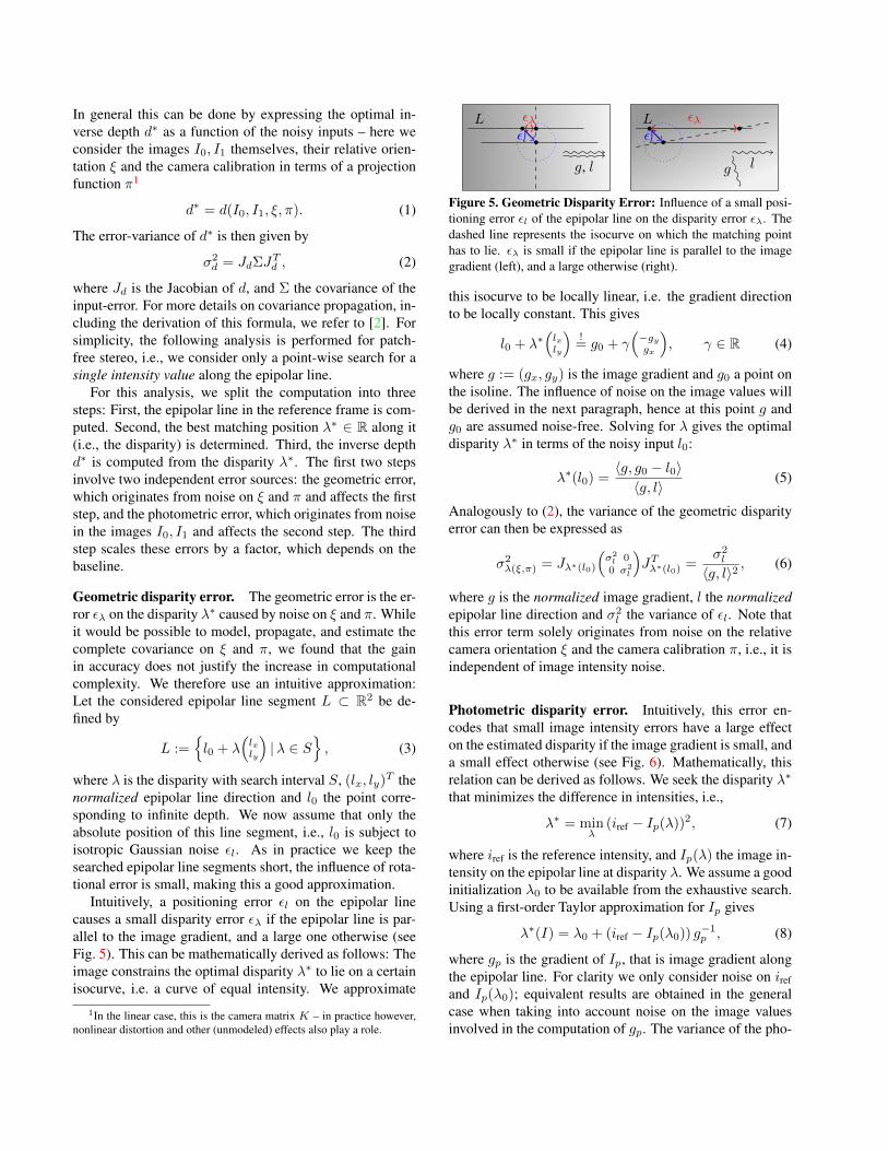
Intuitively, a positioning error εl on the epipolar linecauses a small disparity error ελ if the epipolar line is par-allel to the image gradient, and a large one otherwise (seeFig. 5). This can be mathematically derived as follows: Theimage constrains the optimal disparity λ∗ to lie on a certainisocurve, i.e. a curve of equal intensity. We approximate

1In the linear case, this is the camera matrix K – in practice however,nonlinear distortion and other (unmodeled) effects also play a role.

L ελεl

g, l

L ελεl

lg

Figure 5. Geometric Disparity Error: Influence of a small posi-tioning error εl of the epipolar line on the disparity error ελ. Thedashed line represents the isocurve on which the matching pointhas to lie. ελ is small if the epipolar line is parallel to the imagegradient (left), and a large otherwise (right).

this isocurve to be locally linear, i.e. the gradient directionto be locally constant. This gives

l0 + λ∗(lxly

)!= g0 + γ

(−gygx

), γ ∈ R (4)

where g := (gx, gy) is the image gradient and g0 a point onthe isoline. The influence of noise on the image values willbe derived in the next paragraph, hence at this point g andg0 are assumed noise-free. Solving for λ gives the optimaldisparity λ∗ in terms of the noisy input l0:

λ∗(l0) =〈g, g0 − l0〉〈g, l〉

(5)

Analogously to (2), the variance of the geometric disparityerror can then be expressed as

σ2λ(ξ,π) = Jλ∗(l0)

(σ2l 00 σ2

l

)JTλ∗(l0)

=σ2l

〈g, l〉2, (6)

where g is the normalized image gradient, l the normalizedepipolar line direction and σ2

l the variance of εl. Note thatthis error term solely originates from noise on the relativecamera orientation ξ and the camera calibration π, i.e., it isindependent of image intensity noise.

Photometric disparity error. Intuitively, this error en-codes that small image intensity errors have a large effecton the estimated disparity if the image gradient is small, anda small effect otherwise (see Fig. 6). Mathematically, thisrelation can be derived as follows. We seek the disparity λ∗

that minimizes the difference in intensities, i.e.,

λ∗ = minλ

(iref − Ip(λ))2, (7)

where iref is the reference intensity, and Ip(λ) the image in-tensity on the epipolar line at disparity λ. We assume a goodinitialization λ0 to be available from the exhaustive search.Using a first-order Taylor approximation for Ip gives

λ∗(I) = λ0 + (iref − Ip(λ0)) g−1p , (8)

where gp is the gradient of Ip, that is image gradient alongthe epipolar line. For clarity we only consider noise on irefand Ip(λ0); equivalent results are obtained in the generalcase when taking into account noise on the image valuesinvolved in the computation of gp. The variance of the pho-

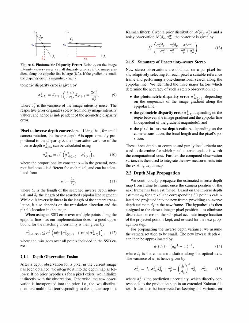
i

λ

Ip

εi

ελ

i

λ

Ipεi

ελ

Figure 6. Photometric Disparity Error: Noise εi on the imageintensity values causes a small disparity error ελ if the image gra-dient along the epipolar line is large (left). If the gradient is small,the disparity error is magnified (right).

tometric disparity error is given by

σ2λ(I) = Jλ∗(I)

(σ2i 00 σ2

i

)Jλ∗(I) =

2σ2i

g2p, (9)

where σ2i is the variance of the image intensity noise. The

respective error originates solely from noisy image intensityvalues, and hence is independent of the geometric disparityerror.

Pixel to inverse depth conversion. Using that, for smallcamera rotation, the inverse depth d is approximately pro-portional to the disparity λ, the observation variance of theinverse depth σ2

d,obs can be calculated using

σ2d,obs = α2

(σ2λ(ξ,π) + σ2

λ(I)

), (10)

where the proportionality constant α – in the general, non-rectified case – is different for each pixel, and can be calcu-lated from

α :=δdδλ, (11)

where δd is the length of the searched inverse depth inter-val, and δλ the length of the searched epipolar line segment.While α is inversely linear in the length of the camera trans-lation, it also depends on the translation direction and thepixel’s location in the image.

When using an SSD error over multiple points along theepipolar line – as our implementation does – a good upperbound for the matching uncertainty is then given by

σ2d,obs-SSD ≤ α2

(minσ2

λ(ξ,π)+ minσ2λ(I)

), (12)

where the min goes over all points included in the SSD er-ror.

2.1.4 Depth Observation Fusion

After a depth observation for a pixel in the current imagehas been obtained, we integrate it into the depth map as fol-lows: If no prior hypothesis for a pixel exists, we initializeit directly with the observation. Otherwise, the new obser-vation is incorporated into the prior, i.e., the two distribu-tions are multiplied (corresponding to the update step in a

Kalman filter): Given a prior distribution N (dp, σ2p) and a

noisy observation N (do, σ2o), the posterior is given by

N

(σ2pdo + σ2

odp

σ2p + σ2

o

,σ2pσ

2o

σ2p + σ2

o

). (13)

2.1.5 Summary of Uncertainty-Aware Stereo

New stereo observations are obtained on a per-pixel ba-sis, adaptively selecting for each pixel a suitable referenceframe and performing a one-dimensional search along theepipolar line. We identified the three major factors whichdetermine the accuracy of such a stereo observation, i.e.,

• the photometric disparity error σ2λ(ξ,π), depending

on the magnitude of the image gradient along theepipolar line,

• the geometric disparity error σ2λ(I), depending on the

angle between the image gradient and the epipolar line(independent of the gradient magnitude), and

• the pixel to inverse depth ratio α, depending on thecamera translation, the focal length and the pixel’s po-sition.

These three simple-to-compute and purely local criteria areused to determine for which pixel a stereo update is worththe computational cost. Further, the computed observationvariance is then used to integrate the new measurements intothe existing depth map.

2.2. Depth Map Propagation

We continuously propagate the estimated inverse depthmap from frame to frame, once the camera position of thenext frame has been estimated. Based on the inverse depthestimate d0 for a pixel, the corresponding 3D point is calcu-lated and projected into the new frame, providing an inversedepth estimate d1 in the new frame. The hypothesis is thenassigned to the closest integer pixel position – to eliminatediscretization errors, the sub-pixel accurate image locationof the projected point is kept, and re-used for the next prop-agation step.

For propagating the inverse depth variance, we assumethe camera rotation to be small. The new inverse depth d1can then be approximated by

d1(d0) = (d−10 − tz)−1, (14)

where tz is the camera translation along the optical axis.The variance of d1 is hence given by

σ2d1 = Jd1σ

2d0J

Td1 + σ2

p =

(d1d0

)4

σ2d0 + σ2

p, (15)

where σ2p is the prediction uncertainty, which directly cor-

responds to the prediction step in an extended Kalman fil-ter. It can also be interpreted as keeping the variance on

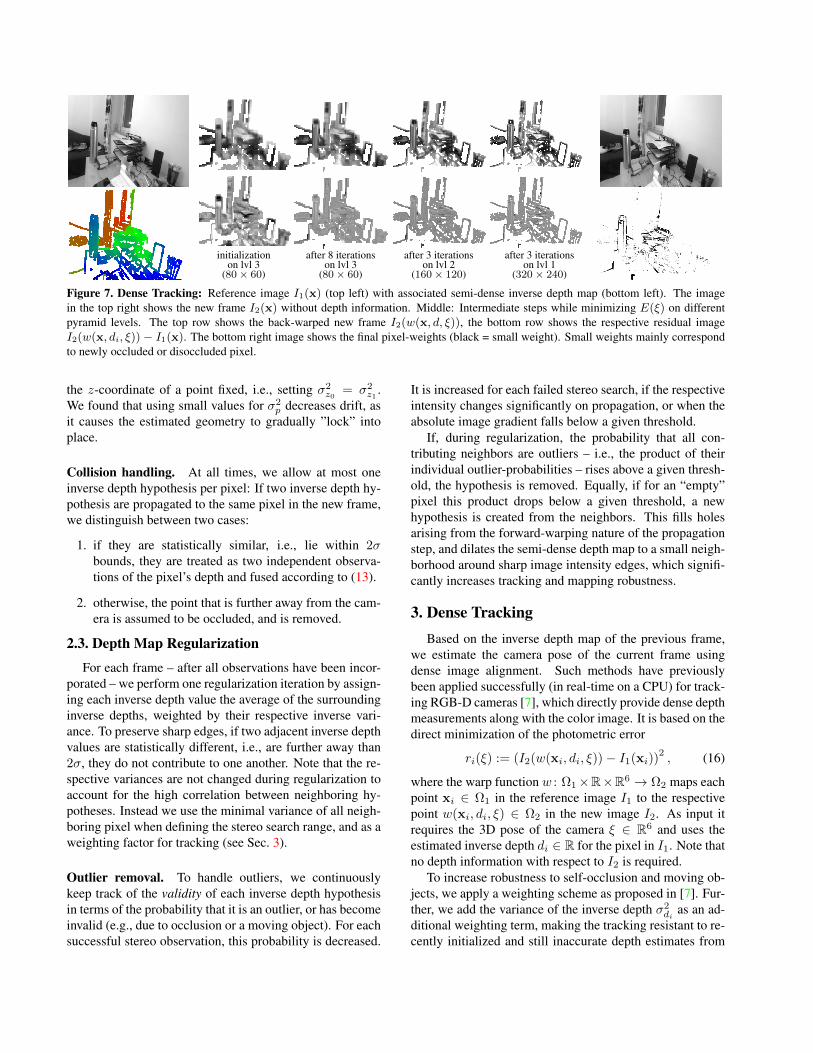
initialization after 8 iterations after 3 iterations after 3 iterationson lvl 3 on lvl 3 on lvl 2 on lvl 1

(80× 60) (80× 60) (160× 120) (320× 240)

Figure 7. Dense Tracking: Reference image I1(x) (top left) with associated semi-dense inverse depth map (bottom left). The imagein the top right shows the new frame I2(x) without depth information. Middle: Intermediate steps while minimizing E(ξ) on differentpyramid levels. The top row shows the back-warped new frame I2(w(x, d, ξ)), the bottom row shows the respective residual imageI2(w(x, di, ξ))− I1(x). The bottom right image shows the final pixel-weights (black = small weight). Small weights mainly correspondto newly occluded or disoccluded pixel.

the z-coordinate of a point fixed, i.e., setting σ2z0 = σ2

z1 .We found that using small values for σ2

p decreases drift, asit causes the estimated geometry to gradually ”lock” intoplace.

Collision handling. At all times, we allow at most oneinverse depth hypothesis per pixel: If two inverse depth hy-pothesis are propagated to the same pixel in the new frame,we distinguish between two cases:

1. if they are statistically similar, i.e., lie within 2σbounds, they are treated as two independent observa-tions of the pixel’s depth and fused according to (13).

2. otherwise, the point that is further away from the cam-era is assumed to be occluded, and is removed.

2.3. Depth Map Regularization

For each frame – after all observations have been incor-porated – we perform one regularization iteration by assign-ing each inverse depth value the average of the surroundinginverse depths, weighted by their respective inverse vari-ance. To preserve sharp edges, if two adjacent inverse depthvalues are statistically different, i.e., are further away than2σ, they do not contribute to one another. Note that the re-spective variances are not changed during regularization toaccount for the high correlation between neighboring hy-potheses. Instead we use the minimal variance of all neigh-boring pixel when defining the stereo search range, and as aweighting factor for tracking (see Sec. 3).

Outlier removal. To handle outliers, we continuouslykeep track of the validity of each inverse depth hypothesisin terms of the probability that it is an outlier, or has becomeinvalid (e.g., due to occlusion or a moving object). For eachsuccessful stereo observation, this probability is decreased.

It is increased for each failed stereo search, if the respectiveintensity changes significantly on propagation, or when theabsolute image gradient falls below a given threshold.

If, during regularization, the probability that all con-tributing neighbors are outliers – i.e., the product of theirindividual outlier-probabilities – rises above a given thresh-old, the hypothesis is removed. Equally, if for an “empty”pixel this product drops below a given threshold, a newhypothesis is created from the neighbors. This fills holesarising from the forward-warping nature of the propagationstep, and dilates the semi-dense depth map to a small neigh-borhood around sharp image intensity edges, which signifi-cantly increases tracking and mapping robustness.

3. Dense TrackingBased on the inverse depth map of the previous frame,

we estimate the camera pose of the current frame usingdense image alignment. Such methods have previouslybeen applied successfully (in real-time on a CPU) for track-ing RGB-D cameras [7], which directly provide dense depthmeasurements along with the color image. It is based on thedirect minimization of the photometric error

ri(ξ) := (I2(w(xi, di, ξ))− I1(xi))2, (16)

where the warp function w : Ω1×R×R6 → Ω2 maps eachpoint xi ∈ Ω1 in the reference image I1 to the respectivepoint w(xi, di, ξ) ∈ Ω2 in the new image I2. As input itrequires the 3D pose of the camera ξ ∈ R6 and uses theestimated inverse depth di ∈ R for the pixel in I1. Note thatno depth information with respect to I2 is required.

To increase robustness to self-occlusion and moving ob-jects, we apply a weighting scheme as proposed in [7]. Fur-ther, we add the variance of the inverse depth σ2

dias an ad-

ditional weighting term, making the tracking resistant to re-cently initialized and still inaccurate depth estimates from

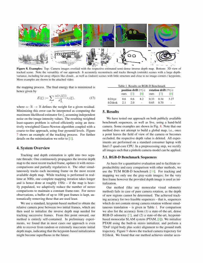
Figure 8. Examples: Top: Camera images overlaid with the respective estimated semi-dense inverse depth map. Bottom: 3D view oftracked scene. Note the versatility of our approach: It accurately reconstructs and tracks through (outside) scenes with a large depth-variance, including far-away objects like clouds , as well as (indoor) scenes with little structure and close to no image corners / keypoints.More examples are shown in the attached video.

the mapping process. The final energy that is minimized ishence given by

E(ξ) :=∑i

α(ri(ξ))

σ2di

ri(ξ), (17)

where α : R → R defines the weight for a given residual.Minimizing this error can be interpreted as computing themaximum likelihood estimator for ξ, assuming independentnoise on the image intensity values. The resulting weightedleast-squares problem is solved efficiently using an itera-tively reweighted Gauss-Newton algorithm coupled with acoarse-to-fine approach, using four pyramid levels. Figure7 shows an example of the tracking process. For furtherdetails on the minimization we refer to [1].

4. System Overview

Tracking and depth estimation is split into two sepa-rate threads: One continuously propagates the inverse depthmap to the most recent tracked frame, updates it with stereo-comparisons and partially regularizes it. The other simul-taneously tracks each incoming frame on the most recentavailable depth map. While tracking is performed in real-time at 30Hz, one complete mapping iteration takes longerand is hence done at roughly 15Hz – if the map is heav-ily populated, we adaptively reduce the number of stereocomparisons to maintain a constant frame-rate. For stereoobservations, a buffer of up to 100 past frames is kept, au-tomatically removing those that are used least.

We use a standard, keypoint-based method to obtain therelative camera pose between two initial frames, which arethen used to initialize the inverse depth map needed fortracking successive frames. From this point onward, ourmethod is entirely self-contained. In preliminary experi-ments, we found that in most cases our approach is evenable to recover from random or extremely inaccurate initialdepth maps, indicating that the keypoint-based initializationmight become superfluous in the future.

Table 1. Results on RGB-D Benchmarkposition drift (cm/s) rotation drift (deg/s)ours [7] [8] ours [7] [8]

fr2/xyz 0.6 0.6 8.2 0.33 0.34 3.27fr2/desk 2.1 2.0 - 0.65 0.70 -

5. Results

We have tested our approach on both publicly availablebenchmark sequences, as well as live, using a hand-heldcamera. Some examples are shown in Fig. 8. Note that ourmethod does not attempt to build a global map, i.e., oncea point leaves the field of view of the camera or becomesoccluded, the respective depth value is deleted. All exper-iments are performed on a standard consumer laptop withIntel i7 quad-core CPU. In a preprocessing step, we rectifyall images such that a pinhole camera-model can be applied.

5.1. RGB-D Benchmark Sequences

As basis for a quantitative evaluation and to facilitate re-producibility and easy comparison with other methods, weuse the TUM RGB-D benchmark [16]. For tracking andmapping we only use the gray-scale images; for the veryfirst frame however the provided depth image is used as ini-tialization.

Our method (like any monocular visual odometrymethod) fails in case of pure camera rotation, as the depthof new regions cannot be determined. The achieved track-ing accuracy for two feasible sequences – that is, sequenceswhich do not contain strong camera rotation without simul-taneous translation – is given in Table 1. For comparisonwe also list the accuracy from (1) a state-of-the-art, denseRGB-D odometry [7], and (2) a state-of-the-art, keypoint-based monocular SLAM system (PTAM, [8]). We initializePTAM using the built-in stereo initializer, and perform a7DoF (rigid body plus scale) alignment to the ground truthtrajectory. Figure 9 shows the tracked camera trajectory forfr2/desk. We found that our method achieves similar accu-

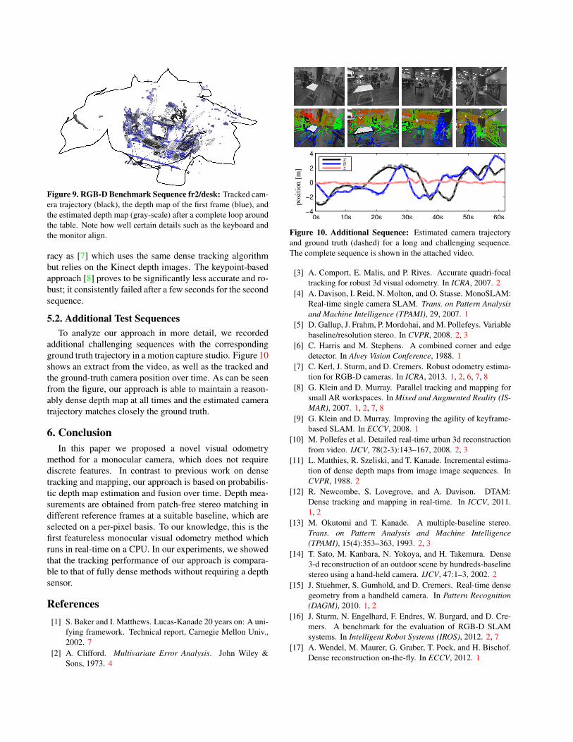
Figure 9. RGB-D Benchmark Sequence fr2/desk: Tracked cam-era trajectory (black), the depth map of the first frame (blue), andthe estimated depth map (gray-scale) after a complete loop aroundthe table. Note how well certain details such as the keyboard andthe monitor align.

racy as [7] which uses the same dense tracking algorithmbut relies on the Kinect depth images. The keypoint-basedapproach [8] proves to be significantly less accurate and ro-bust; it consistently failed after a few seconds for the secondsequence.

5.2. Additional Test SequencesTo analyze our approach in more detail, we recorded

additional challenging sequences with the correspondingground truth trajectory in a motion capture studio. Figure 10shows an extract from the video, as well as the tracked andthe ground-truth camera position over time. As can be seenfrom the figure, our approach is able to maintain a reason-ably dense depth map at all times and the estimated cameratrajectory matches closely the ground truth.

6. ConclusionIn this paper we proposed a novel visual odometry

method for a monocular camera, which does not requirediscrete features. In contrast to previous work on densetracking and mapping, our approach is based on probabilis-tic depth map estimation and fusion over time. Depth mea-surements are obtained from patch-free stereo matching indifferent reference frames at a suitable baseline, which areselected on a per-pixel basis. To our knowledge, this is thefirst featureless monocular visual odometry method whichruns in real-time on a CPU. In our experiments, we showedthat the tracking performance of our approach is compara-ble to that of fully dense methods without requiring a depthsensor.

References[1] S. Baker and I. Matthews. Lucas-Kanade 20 years on: A uni-

fying framework. Technical report, Carnegie Mellon Univ.,2002. 7

[2] A. Clifford. Multivariate Error Analysis. John Wiley &Sons, 1973. 4

0s 10s 20s 30s 40s 50s 60s−4

−2

0

2

4

xyz

posi

tion

[m]

Figure 10. Additional Sequence: Estimated camera trajectoryand ground truth (dashed) for a long and challenging sequence.The complete sequence is shown in the attached video.

[3] A. Comport, E. Malis, and P. Rives. Accurate quadri-focaltracking for robust 3d visual odometry. In ICRA, 2007. 2

[4] A. Davison, I. Reid, N. Molton, and O. Stasse. MonoSLAM:Real-time single camera SLAM. Trans. on Pattern Analysisand Machine Intelligence (TPAMI), 29, 2007. 1

[5] D. Gallup, J. Frahm, P. Mordohai, and M. Pollefeys. Variablebaseline/resolution stereo. In CVPR, 2008. 2, 3

[6] C. Harris and M. Stephens. A combined corner and edgedetector. In Alvey Vision Conference, 1988. 1

[7] C. Kerl, J. Sturm, and D. Cremers. Robust odometry estima-tion for RGB-D cameras. In ICRA, 2013. 1, 2, 6, 7, 8

[8] G. Klein and D. Murray. Parallel tracking and mapping forsmall AR workspaces. In Mixed and Augmented Reality (IS-MAR), 2007. 1, 2, 7, 8

[9] G. Klein and D. Murray. Improving the agility of keyframe-based SLAM. In ECCV, 2008. 1

[10] M. Pollefes et al. Detailed real-time urban 3d reconstructionfrom video. IJCV, 78(2-3):143–167, 2008. 2, 3

[11] L. Matthies, R. Szeliski, and T. Kanade. Incremental estima-tion of dense depth maps from image image sequences. InCVPR, 1988. 2

[12] R. Newcombe, S. Lovegrove, and A. Davison. DTAM:Dense tracking and mapping in real-time. In ICCV, 2011.1, 2

[13] M. Okutomi and T. Kanade. A multiple-baseline stereo.Trans. on Pattern Analysis and Machine Intelligence(TPAMI), 15(4):353–363, 1993. 2, 3

[14] T. Sato, M. Kanbara, N. Yokoya, and H. Takemura. Dense3-d reconstruction of an outdoor scene by hundreds-baselinestereo using a hand-held camera. IJCV, 47:1–3, 2002. 2

[15] J. Stuehmer, S. Gumhold, and D. Cremers. Real-time densegeometry from a handheld camera. In Pattern Recognition(DAGM), 2010. 1, 2

[16] J. Sturm, N. Engelhard, F. Endres, W. Burgard, and D. Cre-mers. A benchmark for the evaluation of RGB-D SLAMsystems. In Intelligent Robot Systems (IROS), 2012. 2, 7

[17] A. Wendel, M. Maurer, G. Graber, T. Pock, and H. Bischof.Dense reconstruction on-the-fly. In ECCV, 2012. 1