Tina Memo No. 2013-004Internal Memo

Semi-automatic Landmark Point Annotation for Geometric

Morphometrics

P.A. Bromiley, A.C. Schunke, H. Ragheb, N.A. Thacker and D. Tautz

Last updated6 / 9 / 2013

Imaging Science and Biomedical Engineering Division,Medical School, University of Manchester,

Stopford Building, Oxford Road,Manchester, M13 9PT.

Semi-automatic Landmark Point Annotation

for Geometric Morphometrics

P.A. Bromiley1, A.C. Schunke2, H. Ragheb1,N.A. Thacker1 and D. Tautz2

1. Imaging Science and Biomedical Engineering, School of Cancer and Imaging Sciences,University of Manchester, Stopford Building, Oxford Road, Manchester M13 9PT, UK.

2. Max Planck Institute for Evolutionary Biology, Department for Evolutionary Genetics,August-Thienemann-Str. 2, 24306 Plon, Germany.

paul.bromiley@manchester.ac.uk

Abstract

Background: In previous work, the authors described a software package for the digitisation of 3Dlandmarks for use in geometric morphometrics. In this paper, we describe extensions to this softwarethat allow semi-automatic location of 3D landmarks, given a database of manually annotated trainingimages. Multi-stage registration was applied to align image patches from the database to a query image,and the results from multiple database images were combined using an array-based voting scheme. Thesoftware automatically highlighted points that had been located with low confidence, allowing manualcorrection.

Results: Evaluation was performed on micro-CT images of rodent skulls for which two independentsets of manual landmark annotations had been performed. This allowed assessment of landmark ac-curacy in terms of both the absolute distance between manual and automatic annotations, and therepeatability of manual and automatic annotation. Automatic annotation attained accuracies equiv-alent to those achievable through manual annotation by an expert for 80% of the points in a typicallandmark annotation process, with significantly higher repeatability.

Conclusions: Whilst user input was required to produce the training data and in a final error cor-rection stage, the software was capable of accelerating the process of landmark identification in 3Ddata by a factor of ten, potentially allowing much larger datasets to be annotated and thus increasingthe statistical power of the results from subsequent processing e.g. Procrustes/principle componentanalysis. The time taken to automatically annotate an image volume was similar to the time requiredby an expert to perform the task manually using AMIRA (www.vsg3d.com/amira). The software isfreely available, under the GNU General Public Licence, from our web-site (www.tina-vision.net).

1 Introduction

There is an increasing level of interest in morphological and morphometric analyses, both for combination withmolecular or ecological data and for a more thorough understanding of forms, e.g. investigations of shape spacesor functional morphology as well as phylogeny reconstruction (e.g. [4, 11, 45, 30]). This is supported by moderndata acquisition methodologies, mainly high resolution CT scans, which provide a multitude of characters on outerand inner surfaces. However, the approaches to landmark assignments have to be adjusted to the special situationof 3D data. 2D images of specimens allow for intersections of a structure, e.g. a suture, and the backgroundof the image, while 3D objects have more degrees of freedom in rotation, so the same points would need to bespecified e.g. as the anterior-most point of a suture. The result is that the process of manual landmark annotationis more difficult, and therefore more time consuming, when 3D data are used. This has significant implications forsubsequent analysis of the data, since the statistical power of any analysis technique, and so the confidence limitson the conclusions, will be dictated in part by the number of data sets that are used.

In [37] the authors described a software package designed to support the process of manual landmark annotationon 3D medical image volumes, with particular reference to micro-CT images. The software presents both 2D and

3D renderings of the image volume, the latter using a fast volume rendering algorithm [26, 25] in order to providethe most informative view of the data possible whilst not imposing requirements for specific graphics hardware,and provides numerous functions designed to accelerate the landmark annotation process. However, the manualinput required to annotate a significant number of landmark points is still considerable. In this work, the authorsdescribe an extension to the software package that supports semi-automatic location of morphological landmarksin a query image.

The problem addressed here was to find the locations of landmarks in a 3D query image volume given a database ofexample image volumes containing similar structures in which the required landmarks had been manually annotatedi.e. to find the mappings from the landmarks in the database images to the corresponding positions in the queryimage. Such mappings constitute sparse transformations from the coordinate systems of the database images tothat of the query image, and so the problem falls into the general domain of registration. Registration is a coreproblem in machine vision and medical image analysis with a correspondingly extensive literature; general reviewsof medical image registration are provided by [23], [46], [32] and [29]), whilst [1], [42] and [41] provide recent reviewsof surface registration algorithms, with particular reference to surfaces represented by point clouds or meshes.

Significant effort has been applied to the problem of non-rigid registration of medical images i.e. of estimating adense deformation field that transforms one image into the coordinate system of another; [39] provides a recentreview. Such methods frequently use a cost function based on two terms; a data term based on the comparison ofimage intensities or derived features, and a regularisation term that constrains the deformation using an assumedphysical model such as viscous fluid flow, elasticity, diffusion etc. However, methods based on free-form deforma-tions of image patches or sub-regions, which attempt to minimise or eliminate the influence of assumed models,have also been investigated. [27] described a hierarchical approach, in which a grid of overlapping sub-regionswere independently registered using cost functions based on mutual information (MI; [12], [43], [44]), normalisedmutual information (NMI; [40]) and the correlation coefficient (CC; [23]), without a regularisation term. A densedeformation field was then estimated from the sparse field of displacement vectors at the region centres by medianfiltering and Gaussian interpolation, introducing an assumption of smoothness. [28] described a method in whichonly those sub-regions with high information content were used. Irregularly spaced sub-regions with high localvariance were selected and registered using the CC; again, a dense deformation field was estimated from the sparsefield of displacement vectors at the region centres by interpolation with thin-plate splines (TPS; [5]), introduc-ing a smoothness assumption based on minimising the bending energy. [38] extended this approach by analysingthe quality of the optimum alignment found for each sub-region using the second derivative of the cost function.Sub-regions on a regular grid were independently aligned using a NMI cost function, and an elastic relaxation wasapplied depending on the alignment quality: when the cost function exhibited a clear optimum, no relaxation wasapplied; a combination of data and elastic terms were applied when the optimum was degenerate; and the relax-ation was performed with no data term when the optimum was indistinct or absent. B-spline interpolation wasthen applied to estimate a dense deformation field. [19] adopted a similar approach, and provided a mathematicalframework for the use of eigenvectors of the Hessian matrix of the cost function for estimation of alignment quality,in terms of a Taylor series expansion of the shape of the cost function at the optimum. This method can also bederived within a statistical framework in terms of the minimum variance bound ([7, 8]). Finally, [24] describeda patch-based registration method inspired by patch-based, multi-atlas segmentation algorithms. The methodassumed that the deformation fields between a set of training images and a template were known; a dictionaryof patches from the training images, and their deformations, was then constructed. A query image could then beregistered to the template by selecting patches around points of high information (high Canny edge detector [10]responses were used), finding the most similar patches in the dictionary, and constructing a weighted combina-tion of the deformations of those dictionary patches. A dense deformation field was then constructed using TPSinterpolation, again introducing a smoothness assumption.

Significant effort has also been applied to the problem of automatic landmark point location in 2D images withinthe computer vision field. One popular approach has been the use of statistical shape models, in algorithms such asthe Active Shape Model (ASM) [16, 17] and related work. In the original work, a set of training images were alignedinto a common coordinate system and the coordinates of the landmarks from each training image, in this referenceframe, were concatenated to form a single, high-dimensional vector, such that the complete set of training imagesdefined a point cloud in a high-dimensional space. A principle component analysis (PCA) was applied to extractthe major modes of variation of this point cloud. The shape model then consisted of two components; a linearcombination of these modes, weighted by a set of shape parameters, and a global rigid transformation that locatedthe model within an image. The model was fitted to a query image by optimising the weights and transformationmodel parameters in order to maximise the image intensity gradient at the landmark point positions i.e. assumingthat landmarks would be located on edges in the image. The Active Appearance Model (AAM) [14] extendedthe same approach to include image intensities, thus producing a model of both shape and appearance. Laterdevelopments, for example the Constrained Local Model (CLM) [18], replaced the global appearance model with

3

a set of texture patches around the landmark points. Fitting consisted of a registration of image patches learnedfrom the training data, or reconstructed from the appearance model, to the query image, with the shape modelused as a constraint during optimisation in order to ensure that the relative locations of the patches represented ahigh-probability shape given the training data. AAMs and related algorithms learn a model directly from trainingdata with no other input. However alternative approaches that incorporate a model of an object as a collection ofinterconnected parts, e.g. the Pictorial Structure Model (PSM) [20], have also been developed. Whilst most efforthas been focused on the application of these techniques to 2D images of faces or objects in natural scenes, theyhave also been applied to 3D medical image data for purposes such as segmentation; see [22] for a recent review.

The methods described above all perform a registration by optimising a cost function that measures the similaritybetween the intensities of two images, or image patches, regularised using a model that describes the probabilityof a given deformation. They exist on a spectrum of model complexity, from very limited models assuming onlythat the deformation field is smooth and continuous, through full physical (e.g. elastic) models of the allowabledeformations, to AAMs that are bootstrapped from training data. However, several considerations militatedagainst using a model-based regularisation in the work described here. Most importantly, the aim was to producelandmarks for geometric morphometrics, which would be analysed with the standard techniques used in that areaof research, including Procrustes analysis followed by PCA and interpolation between landmarks using thin-platesplines i.e. the same techniques used in model construction for deformable registration. Therefore, the subsequentanalysis would be capable of recovering the registration model; any mode of shape variation in the data thatwas not included in the model would therefore directly affect the results of the subsequent analysis. In practice,such unmodeled modes of variation would always be present. For example, the training data for an AAM wouldneed to exhibit all possible shape variation within the relevant shapes in order to guarantee full coverage; thiswould make the training set prohibitively large. Similarly, a smoothness assumption would not allow points ofinfinite curvature in the deformation field. However, such points could be present at the interface between slidingsurfaces e.g. the points of contact between the upper and lower molar rows, which would be relevant landmarklocations for many studies comparing morphology with ecology. Furthermore, the bootstrapped models used inAAMs and related algorithms require extensive offline training; since the aim here was to maximally acceleratethe landmark annotation process, a method without this requirement was preferred. Finally, much of the workon AAMs and related algorithms has focused on 2D images of natural scenes, where out-of-plane rotations canresult in significant deformations between the source and target images that cannot be recovered using a 2Dtransformation. The algorithm described here was designed for use on high-resolution, 3D, tomographic medicalimages, where the problem of out-of-plane rotations is not present and so the significance of the regularisation termis reduced, although not eliminated.

The work described here adopted the hierarchical, patch-based registration approach whilst avoiding any model-based shape constraint. This approach proved successful in earlier work on automatic landmark annotation formorphometric analysis of microscope images of fly wings i.e. 2D images of planar objects with no out-of-planerotations [34, 35]. The software required a database of images similar to the query image, in which the requiredlandmarks had been manually annotated. In the absence of regularisation, a multi-stage registration approachwas developed in order to compensate for shape variations between the database and query images, which wouldnecessarily be present. The initial stages operated on the whole image, and so were affected by shape variations.However, the results from the initial stages were used only to initialise later stages operating on texture patchesaround each landmark. Multiple patch-based stages with reducing patch sizes were used, with the intention thatthe effect of global shape variation would be reduced as the patches became smaller. Automatic image registrationalgorithms are typically incapable of dealing with gross misalignments e.g. where the images are rotated by180◦with respect to one another, and so manual intervention was required to provide an initialisation. In the workdescribed here, four non-coplanar landmark points in each volume were used for this purpose. Future versionsof the software could potentially achieve the same end by prompting the user to rotate the image to a standardorientation in a 3D rendering of the data, and this stage of the algorithm can be omitted completely if care istaken during sample preparation, such that the specimens are in approximately the same orientation in all imagevolumes used. The point-based stage of the registration minimised the RMS distances between the registrationpoints. All image-based stages minimised the χ2 of the scaled intensity gradients in the database and query images;the scaling provided some independence to variations in scanner parameters and average bone density, and wasestimated using maximum likelihood after the point-based stage of registration.

Each database image produced one estimate of the location of each landmark in the query image; these werecombined to generate the final estimated landmark location. However, significant shape variation between adatabase image and the query image close to a landmark might cause the registration for that image and landmarkto fail i.e. the results might be contaminated with outliers. Therefore, a robust alternative to simple approachessuch as averaging was required. Since the introduction of the generalised Hough transform [2], array based votingschemes have been shown to be effective for locating structures in images. In particular, several recent papers (e.g.

4

[21, 15]) have used Random Forests [6] to locate structures in images, combining the estimates from each tree in avoting array. A similar approach was adopted here; the estimated positions of a given landmark from each databaseentry cast votes into a 3D array, which was then convolved with a Gaussian kernel to approximate the random erroron the estimates. Outliers resulting from failed registrations formed a broad background distribution, whilst pointsfrom the signal distribution (i.e. successful registrations) were randomly scattered around the true location of thelandmark point in the query image according to the random error on the estimation process, and so contributedto a single, dominant peak in the voting array. The most significant mode in the smoothed array was taken as theestimated location for the landmark. This provided a degree of robustness to outliers; however, situations mightstill occur in which no element of the database provided a good estimate of the landmark location. Therefore,a robust outlier detection method was applied to the final estimated locations, based on testing for consistencybetween the result from the array-based voting and the estimated χ2 per degree of freedom on the points thatcontributed to the array.

2 The Multi-Stage Registration Algorithm

The automatic landmark annotation process was based on a hierarchical, free-form registration of image patchesfrom the database to the query image. An initial alignment was derived from four landmark points, by minimisingthe root-mean-squared (RMS) distances between corresponding points over a nine-parameter affine transformation(i.e. 3D translation, rotation and scale) using the simplex algorithm [31]. An automated check was implementedto ensure that the points were not coplanar. This point-based registration could have been decomposed into in-dividual transformations, deriving the translation parameters by aligning the centroids of the four points and thescaling parameters from the standard deviations of the points, leaving only the rotation to be obtained throughoptimisation. However, in practice all nine parameters of the transformation model were obtained via the optimi-sation, so that the distance between the centroids of the points in each registered image volume could be used asa semi-independent, automated check.

Once the initial manual alignment had been obtained, it was used to initialise a multi-stage automatic registra-tion process. The first stage was performed on the entire image volume, and optimised a nine-parameter affinetransformation using the simplex algorithm [31]. The latter stages operated on patches of image data around eachlandmark point. As described above, the intention was to terminate the process with patches small enough that theeffects of shape variation between the database and query images were minimised. However, registration of smallpatches had a correspondingly small capture range: in preliminary work, a single stage of patch-based registrationproved to be insufficient to attain accuracies equivalent to manual annotation. Therefore, additional stages ofpatch-based registration were included, with the patch size reduced between each stage; an empirical evaluation ofaccuracy and time vs. the number of registration stages was performed, and the optimal number of patch-basedstages was shown to be three, for a total of five stages of registration including the point-based initialisation andthe global, image-based stage (see Appendix C). Some experiments in geometric morphometrics may include land-marks specified as the extremal points on curved surfaces from certain view directions. The inclusion of rotation inthe patch-based registration would destabilise the registration in such cases (e.g. registration of an arc of a circleto that circle is degenerate over rotation, but not translation or scaling). Therefore, the transformation modelused in the patch-based stages of registration consisted of 3D translation and scaling. Each stage of registrationwas initialised using the concatenation of the transformation matrices from all previous stages. However, a simplecheck was included to prevent problems with fit failures; if the result from any stage of registration generated aprojected location that lay outside the boundaries of the query image volume, then the parameters of that stagewere set to an identity transformation.

Since a nine-parameter affine transformation model was used, the problem was over-determined with realistic patchsizes. Therefore, rather than using cuboids from the data as image patches, 2D slices aligned to the major axes ofthe image volume and centred on the landmark points were used; in the first stage, operating on the entire imagevolumes, the slices were taken through the centre point of the volumes. This considerably reduced the amountof data included in the cost function calculation, and so reduced the processor time required without significantimpact on accuracy.

The cost function for all automatic registration stages was the χ2 per degree of freedom of the scaled images orimage patches (a derivation is provided in Appendix A)

χ2 =1

(N −D)

∑

v

(Jv − γIv)2

σ2J + σ2

Iγ2

where γ =|J ||I| (1)

where, assuming without loss of generality that I is the source (database) image and J the target (query) image,Ji is the value of voxel i in the target image, Ii is the value of the corresponding voxel in the transformed source

5

image after re-sampling onto the voxel grid of the target image using an interpolation algorithm, N is the numberof voxels in the images or image patches, σI and σJ are the standard deviations of the noise on the scaled images orpatches, D is the number of transformation model parameters being optimised, and γ is a scaling factor, providingsome degree of independence to differences in scanner parameters and average bone density. Trilinear interpolationwas used in the resampling. The scaling factor was obtained through a maximum-likelihood based approach (seeAppendix A). Inevitably, the scaling could be computed only from aligned images. Therefore, it was computedafter the point-based stage of registration, and then remained fixed through all of the image-based registrationstages.

In order to reduce the noise on the images and thus provide a smoother cost function, reducing the probabilitythat the optimisation would become trapped in a local minimum, Gaussian smoothing was applied to all imagepatches prior to registration. The kernel was truncated at three standard deviations from the mean and, in orderto ensure that no edge effects were present, a boundary equal to three standard deviations of the smoothing kernelwas added around all stored image patches and included in the smoothing, but excluded from the χ2 calculation,thus ensuring that all smoothed voxels contributing the the χ2 were calculated from equal numbers of un-smoothedvoxels.

Rather than operating directly on the image intensities, the cost function was applied to image intensity gradientsin order to provide further robustness to differences in average bone density or scanner parameters. The χ2 perdegree of freedom for each gradient component was calculated separately and then summed, in order to avoidthe intensity-dependent noise term that would be required if gradient magnitude were used. Therefore, the finalχ2 per degree of freedom was calculated from six image patches; the horizontal and vertical gradient componentsof each of the three orthogonal patches through each landmark point. Note that N in Eq. 1 refers to the totalnumber of voxels included in the orthogonal patches, not the total number in the derivative patches, since the x-and y-derivative images of each patch were obtained from the same original data.

Explicit inclusion of the noise term in the cost function allowed the χ2 per degree of freedom at the end of theregistration to be used as a check on registration error, through comparison to the χ2 distribution. The noise onthe original images was estimated from the width of zero crossings in horizontal and vertical gradient histograms[33]. Smoothing reduced the noise by a factor of 4πσ2

K where σK was the standard deviation of the smoothingkernel [13] (see Appendix B). Image gradients were calculated by finite differencing, introducing a further factorof 1/2 into the noise calculation.

Particular care was required in cases where part of an image patch lay outside the volume. Simply ignoring suchregions would bias the registration towards moving the patches almost completely outside the query image volumein cases where there was any shape difference. Therefore, any regions lying outside the image volumes were zero-padded and included in the χ2 calculation. Furthermore, image masks were generated for all patches, recordingthe zero-padded regions. The cost function was then calculated as three separate terms i.e. one for voxels lyinginside both volumes, one for voxels where the I image voxel was zero padded, and one for voxels where the J imagevoxel was zero padded; the fourth combination, where both voxels were zero-padded, was identically zero. Thecorrect noise term was used in each case (σ2

J + γ2σ2I , γ

2σ2I , and σ2

J respectively, divided by the correction factorsfor smoothing and differentiation). These three χ2 terms were then summed prior to division by the number ofdegrees of freedom, the total number of voxels included in all three terms minus the number of parameters in thetransformation model.

Array-based Voting

The result from the various stages of registration was a projected location, in the coordinate system of the queryimage, for each landmark point in each database entry. The multiple estimates for each landmark were thencombined in order to generate a single, final estimate of the location of that landmark in the query image. Anysimple approach, such as taking the mean or median of the multiple estimates, would include an implicit assumptionthat the estimates were drawn from a single distribution. In practice, however, the possibility of registrationfailures due to shape differences between the volumes, or local minima in the cost function due to noise, remained.Therefore, an alternative approach inspired by the array-based voting used in methods such as Hough transformswas implemented. A 3D voting array was constructed, each point cast a vote into that array as a Kroneckerdelta function, and the array was then smoothed using a Gaussian kernel. The position of the most significantmode in the smoothed array was then used as the final estimate of the landmark point location. This procedureavoided the logical AND implied in a simple mean or median, instead using a logical OR i.e. finding the mostprobable location for the final estimate based on any sub-set of the multiple estimates, allowing outliers to beignored. The kernel size was a free parameter of the algorithm (see Appendix C); however, future development ofthe algorithm could potentially include the implementation of probabilistic voting, by estimating the covariance

6

matrix on the registration parameters using the techniques described in [7, 8], applying error propagation tocalculate the covariance matrix on the spatial location of the projected point, and casting votes in the arrayaccording to this matrix.

Prior to creation of the voting array for each landmark point, the projected locations of the corresponding databasepoints in the coordinate system of the query image were compared to the boundaries of that image; any point lyingoutside the boundary plus a border of three times the standard deviation of the smoothing kernel was omittedfrom the voting process, in order to prevent problems with severe outliers, on the basis that these points could notcontribute to a valid final estimate in any case. The size of the array was then determined by finding the maximumand minimum x, y and z values of the projected locations for the remaining points.

Outlier Detection

In order for the final algorithm to have any utility, it was essential that it should provide a reliable indication ofthe accuracy of automatic annotations; otherwise, much of the manual interaction that it was intended to replacewould be re-introduced through a requirement for manual inspection of the results. An outlier detection methodwith an extremely low false positive rate i.e. an extremely low number of outliers flagged as accurate annotations,was therefore required.

If a given database image patch formed a perfect model of the corresponding query image patch, then the onlysource of errors on the optimised transformation model parameters would be the random noise on the images.Since a maximum likelihood estimator was used as the registration cost function, the minimum variance bound(MVB; [7, 8]) could be applied to estimate this distribution; error propagation could then be applied to findthe distribution of the estimated landmark locations. However, in practice there will always be shape differencesbetween the database and query images, introducing a systematic error onto each patch registration. Assumingthese systematic errors to be uncorrelated across the database images, they introduce a secondary distribution i.e.the multiple estimated landmark locations generated from the database images will be randomly scattered aroundthe true landmark location in the query image according to a distribution dependent on random shape differences(which could be termed “shape noise”). This will add to the distribution due to random image noise, and so theMVB will provide an underestimate of the true distribution of the estimated landmark locations.

As stated above, [38] and [19] developed a method that measured the shape of the cost function around the optimumusing the eigenvectors of the Hessian matrix, allowing the rejection of results where shape differences destabilisedthe registration to the point where there was no clear optimum. However, this method was limited to analysisof the cost functions for individual registrations. In the work described here, the multiple registration results foreach landmark supported an analysis of the distribution of registration parameters induced by shape variationbetween the database images. The number of samples available was too small to allow a full characterisation ofthe distribution; therefore, unreliable results were identified through an analysis of the available point estimates.The individual registration results were first sorted into order based on the χ2 per degree of freedom at the endof the registration process. A threshold was then placed on the distance between the results and the final locationgenerated by the array-based voting. The threshold and the number of comparisons performed were free parametersof the algorithm (see Appendix C); in practice, comparison to three points proved optimal. Any final location forwhich any one of the three registration results with the lowest χ2 per degree of freedom was more distant than thethreshold was flagged as a potential outlier. The technique therefore imposed a requirement that the patches whichwere estimated to provide the best models of the query image patch, based on their χ2 per degree of freedom,formed a distribution within the voting array no broader than the threshold.

Software

The semi-automatic point location algorithm was implemented within the TINA Geometric Morphometrics toolkit,which also includes the TINA Manual Landmarking tool [37], and algorithms that perform quantitative shapeanalysis with weighted covariance estimates for increased statistical efficiency [36]. This package has been madeavailable as free and open source software (FOSS) under the GNU General Public Licence (www.gnu.org) and,together with the User Guide [9], can be obtained via the TINA web-site (www.tina-vision.net). Figure 1 showsa screen-shot of the software in operation. The 3D renderings and associated landmark annotations are shown inmore detail in Figure 2.

7

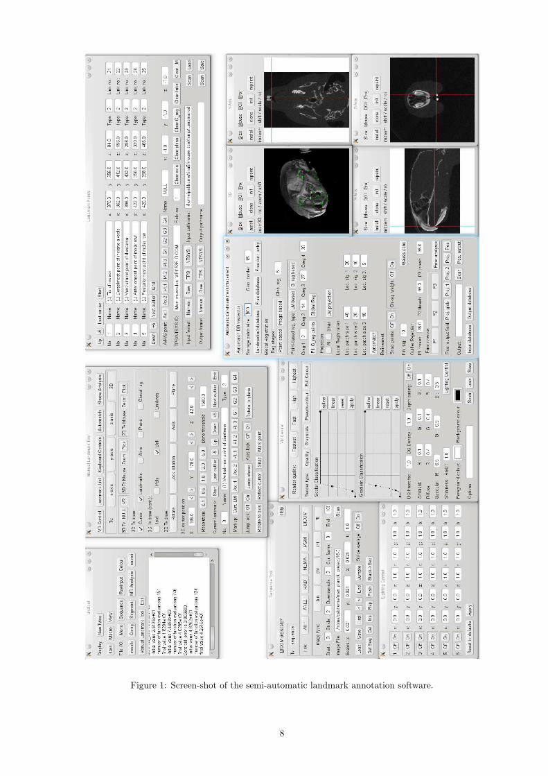
Figure 1: Screen-shot of the semi-automatic landmark annotation software.

8

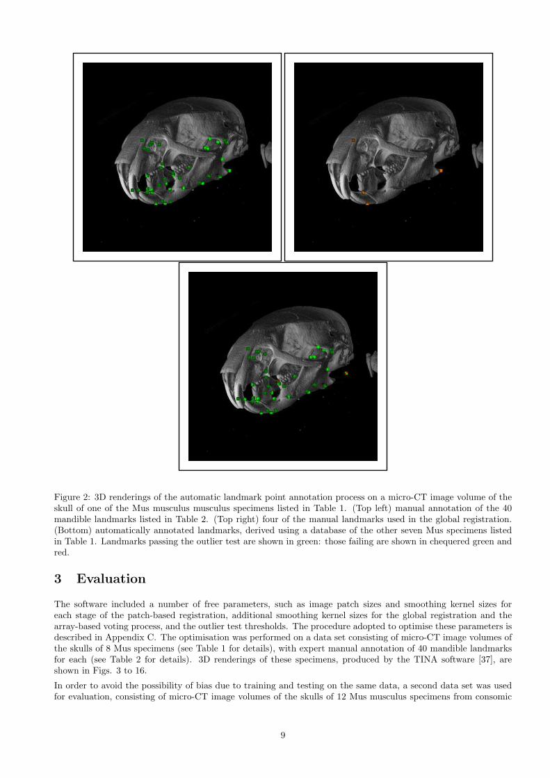
Figure 2: 3D renderings of the automatic landmark point annotation process on a micro-CT image volume of theskull of one of the Mus musculus musculus specimens listed in Table 1. (Top left) manual annotation of the 40mandible landmarks listed in Table 2. (Top right) four of the manual landmarks used in the global registration.(Bottom) automatically annotated landmarks, derived using a database of the other seven Mus specimens listedin Table 1. Landmarks passing the outlier test are shown in green: those failing are shown in chequered green andred.

3 Evaluation

The software included a number of free parameters, such as image patch sizes and smoothing kernel sizes foreach stage of the patch-based registration, additional smoothing kernel sizes for the global registration and thearray-based voting process, and the outlier test thresholds. The procedure adopted to optimise these parameters isdescribed in Appendix C. The optimisation was performed on a data set consisting of micro-CT image volumes ofthe skulls of 8 Mus specimens (see Table 1 for details), with expert manual annotation of 40 mandible landmarksfor each (see Table 2 for details). 3D renderings of these specimens, produced by the TINA software [37], areshown in Figs. 3 to 16.

In order to avoid the possibility of bias due to training and testing on the same data, a second data set was usedfor evaluation, consisting of micro-CT image volumes of the skulls of 12 Mus musculus specimens from consomic

9

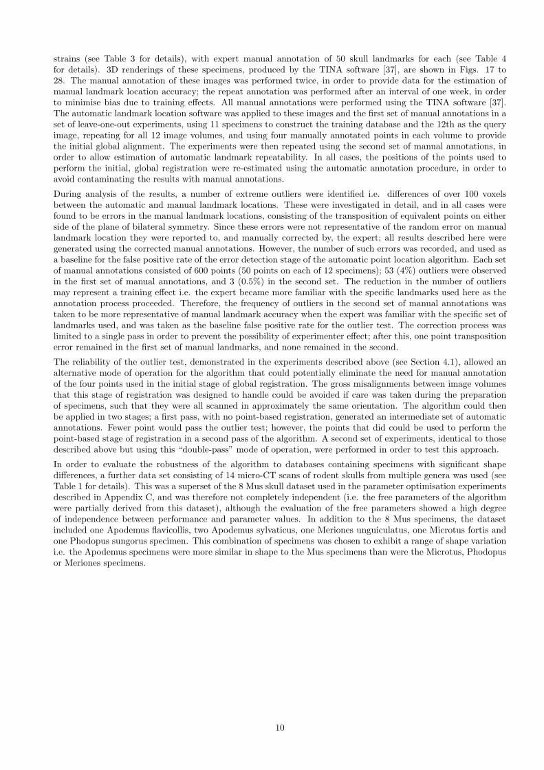
strains (see Table 3 for details), with expert manual annotation of 50 skull landmarks for each (see Table 4for details). 3D renderings of these specimens, produced by the TINA software [37], are shown in Figs. 17 to28. The manual annotation of these images was performed twice, in order to provide data for the estimation ofmanual landmark location accuracy; the repeat annotation was performed after an interval of one week, in orderto minimise bias due to training effects. All manual annotations were performed using the TINA software [37].The automatic landmark location software was applied to these images and the first set of manual annotations in aset of leave-one-out experiments, using 11 specimens to construct the training database and the 12th as the queryimage, repeating for all 12 image volumes, and using four manually annotated points in each volume to providethe initial global alignment. The experiments were then repeated using the second set of manual annotations, inorder to allow estimation of automatic landmark repeatability. In all cases, the positions of the points used toperform the initial, global registration were re-estimated using the automatic annotation procedure, in order toavoid contaminating the results with manual annotations.

During analysis of the results, a number of extreme outliers were identified i.e. differences of over 100 voxelsbetween the automatic and manual landmark locations. These were investigated in detail, and in all cases werefound to be errors in the manual landmark locations, consisting of the transposition of equivalent points on eitherside of the plane of bilateral symmetry. Since these errors were not representative of the random error on manuallandmark location they were reported to, and manually corrected by, the expert; all results described here weregenerated using the corrected manual annotations. However, the number of such errors was recorded, and used asa baseline for the false positive rate of the error detection stage of the automatic point location algorithm. Each setof manual annotations consisted of 600 points (50 points on each of 12 specimens); 53 (4%) outliers were observedin the first set of manual annotations, and 3 (0.5%) in the second set. The reduction in the number of outliersmay represent a training effect i.e. the expert became more familiar with the specific landmarks used here as theannotation process proceeded. Therefore, the frequency of outliers in the second set of manual annotations wastaken to be more representative of manual landmark accuracy when the expert was familiar with the specific set oflandmarks used, and was taken as the baseline false positive rate for the outlier test. The correction process waslimited to a single pass in order to prevent the possibility of experimenter effect; after this, one point transpositionerror remained in the first set of manual landmarks, and none remained in the second.

The reliability of the outlier test, demonstrated in the experiments described above (see Section 4.1), allowed analternative mode of operation for the algorithm that could potentially eliminate the need for manual annotationof the four points used in the initial stage of global registration. The gross misalignments between image volumesthat this stage of registration was designed to handle could be avoided if care was taken during the preparationof specimens, such that they were all scanned in approximately the same orientation. The algorithm could thenbe applied in two stages; a first pass, with no point-based registration, generated an intermediate set of automaticannotations. Fewer point would pass the outlier test; however, the points that did could be used to perform thepoint-based stage of registration in a second pass of the algorithm. A second set of experiments, identical to thosedescribed above but using this “double-pass” mode of operation, were performed in order to test this approach.

In order to evaluate the robustness of the algorithm to databases containing specimens with significant shapedifferences, a further data set consisting of 14 micro-CT scans of rodent skulls from multiple genera was used (seeTable 1 for details). This was a superset of the 8 Mus skull dataset used in the parameter optimisation experimentsdescribed in Appendix C, and was therefore not completely independent (i.e. the free parameters of the algorithmwere partially derived from this dataset), although the evaluation of the free parameters showed a high degreeof independence between performance and parameter values. In addition to the 8 Mus specimens, the datasetincluded one Apodemus flavicollis, two Apodemus sylvaticus, one Meriones unguiculatus, one Microtus fortis andone Phodopus sungorus specimen. This combination of specimens was chosen to exhibit a range of shape variationi.e. the Apodemus specimens were more similar in shape to the Mus specimens than were the Microtus, Phodopusor Meriones specimens.

10

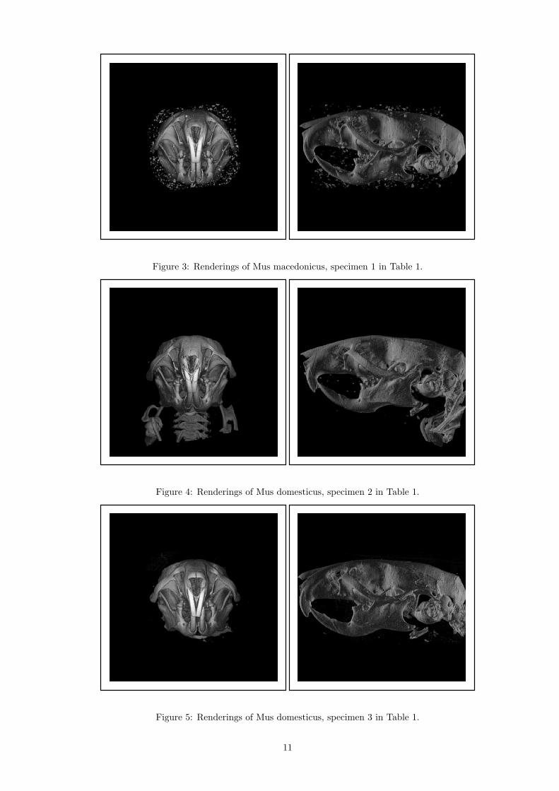
Figure 3: Renderings of Mus macedonicus, specimen 1 in Table 1.

Figure 4: Renderings of Mus domesticus, specimen 2 in Table 1.

Figure 5: Renderings of Mus domesticus, specimen 3 in Table 1.

11

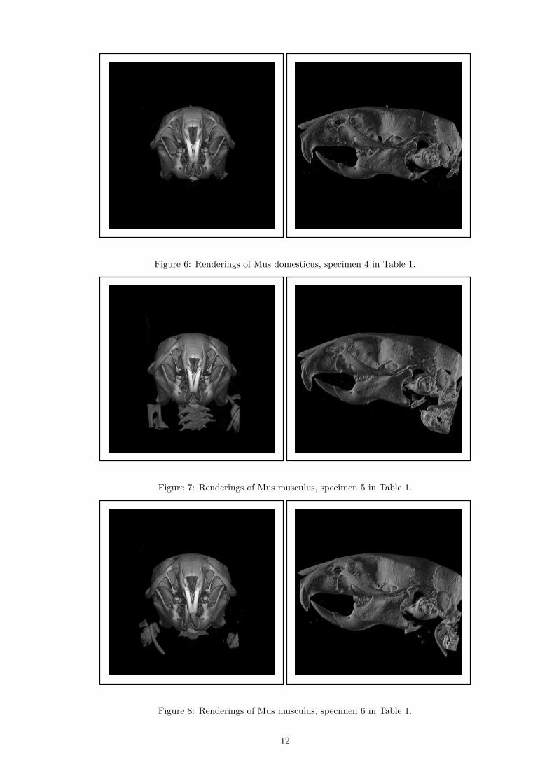
Figure 6: Renderings of Mus domesticus, specimen 4 in Table 1.

Figure 7: Renderings of Mus musculus, specimen 5 in Table 1.

Figure 8: Renderings of Mus musculus, specimen 6 in Table 1.

12

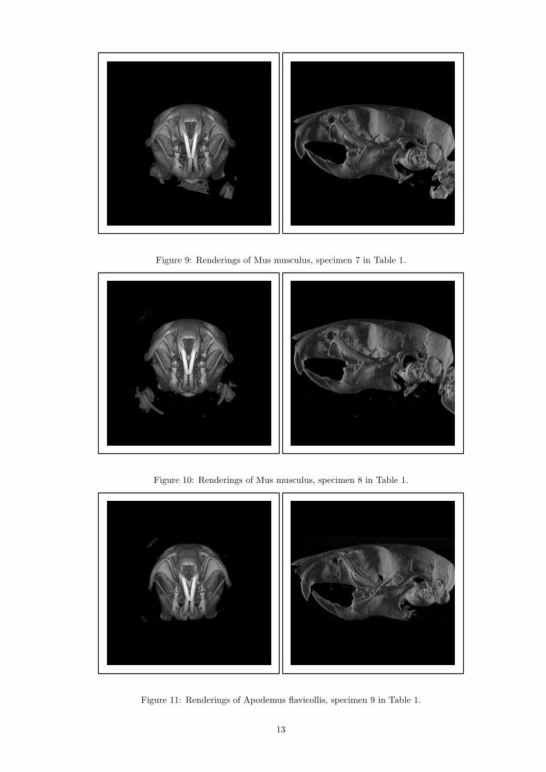
Figure 9: Renderings of Mus musculus, specimen 7 in Table 1.

Figure 10: Renderings of Mus musculus, specimen 8 in Table 1.

Figure 11: Renderings of Apodemus flavicollis, specimen 9 in Table 1.

13

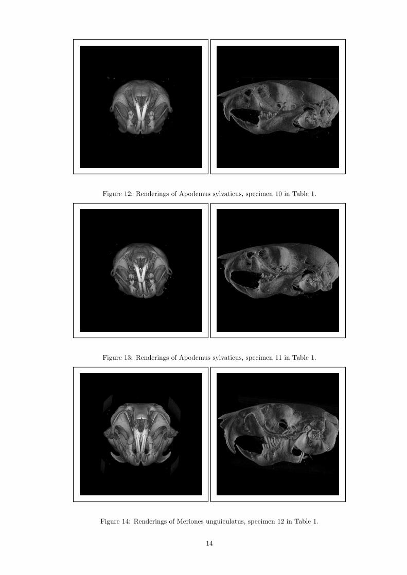
Figure 12: Renderings of Apodemus sylvaticus, specimen 10 in Table 1.

Figure 13: Renderings of Apodemus sylvaticus, specimen 11 in Table 1.

Figure 14: Renderings of Meriones unguiculatus, specimen 12 in Table 1.

14

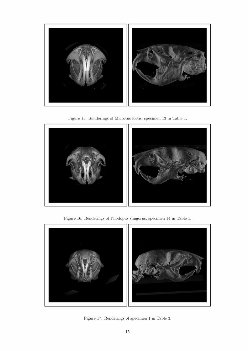
Figure 15: Renderings of Microtus fortis, specimen 13 in Table 1.

Figure 16: Renderings of Phodopus sungorus, specimen 14 in Table 1.

Figure 17: Renderings of specimen 1 in Table 3.

15

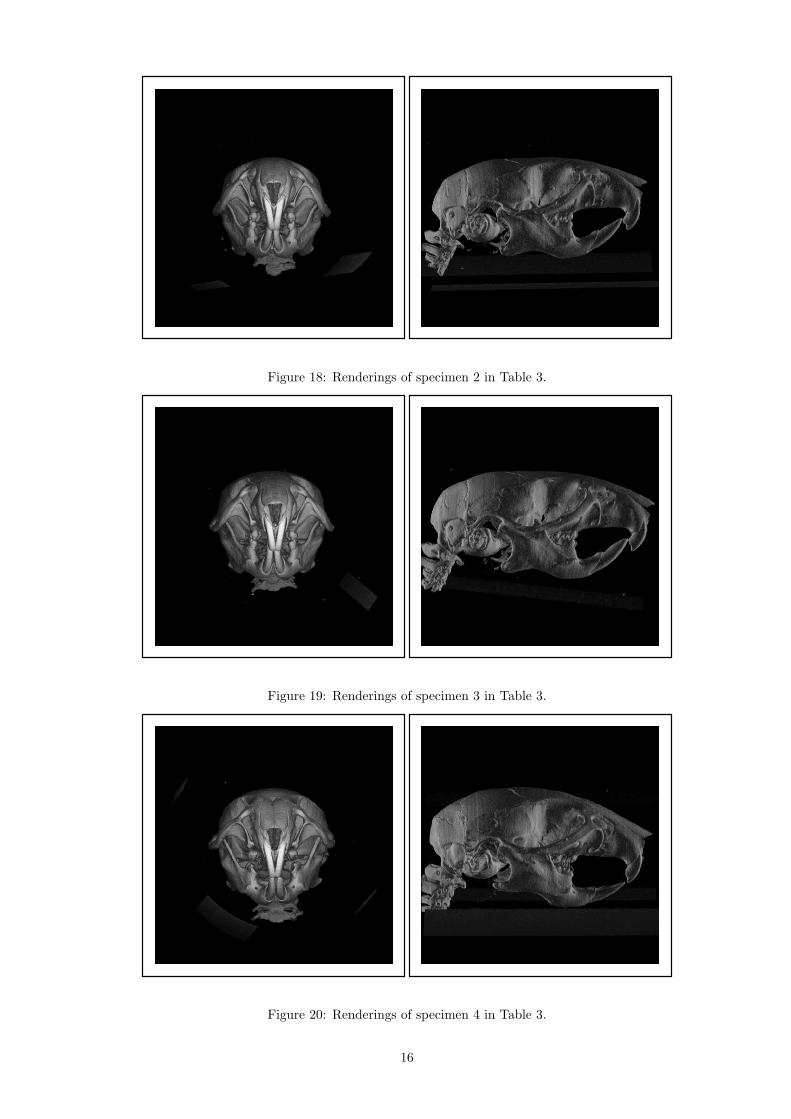
Figure 18: Renderings of specimen 2 in Table 3.

Figure 19: Renderings of specimen 3 in Table 3.

Figure 20: Renderings of specimen 4 in Table 3.

16

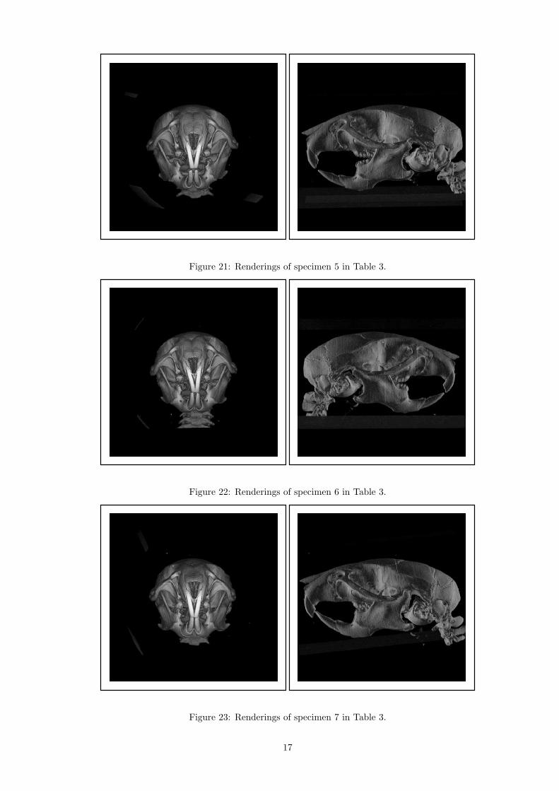
Figure 21: Renderings of specimen 5 in Table 3.

Figure 22: Renderings of specimen 6 in Table 3.

Figure 23: Renderings of specimen 7 in Table 3.

17

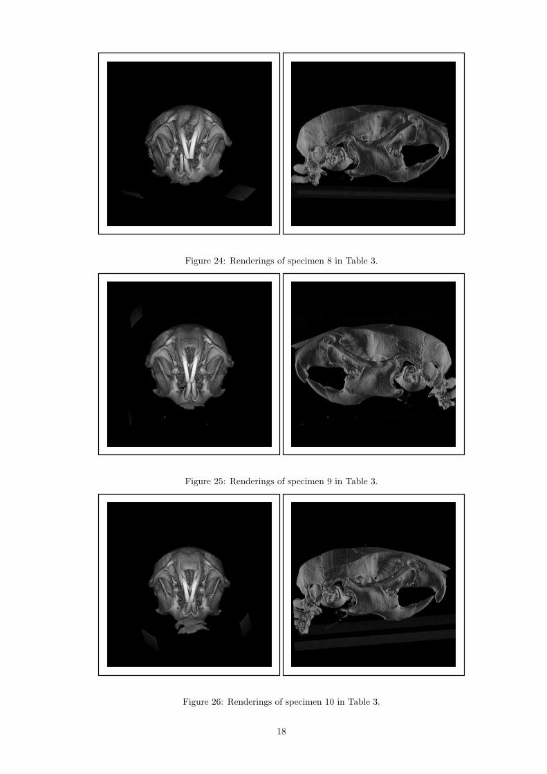
Figure 24: Renderings of specimen 8 in Table 3.

Figure 25: Renderings of specimen 9 in Table 3.

Figure 26: Renderings of specimen 10 in Table 3.

18

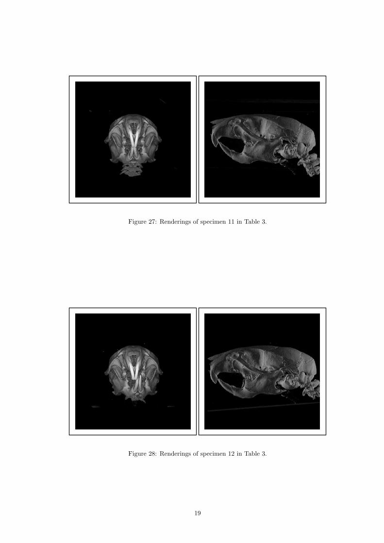
Figure 27: Renderings of specimen 11 in Table 3.

Figure 28: Renderings of specimen 12 in Table 3.

19

Specimen Description1 Mus macedonicus (Macedonian mouse)2 Mus musculus domesticus (House mouse)3 Mus musculus domesticus (House mouse)4 Mus musculus domesticus (House mouse)5 Mus musculus musculus (House mouse)6 Mus musculus musculus (House mouse)7 Mus musculus musculus (House mouse)8 Mus musculus musculus (House mouse)9 Apodemus flavicollis (Yellow-necked mouse)10 Apodemus sylvaticus (Wood mouse)11 Apodemus sylvaticus (Wood mouse)12 Meriones unguiculatus (Mongolian gerbil)13 Microtus fortis (Reed vole)14 Phodopus sungorus (Djungarian hamster)

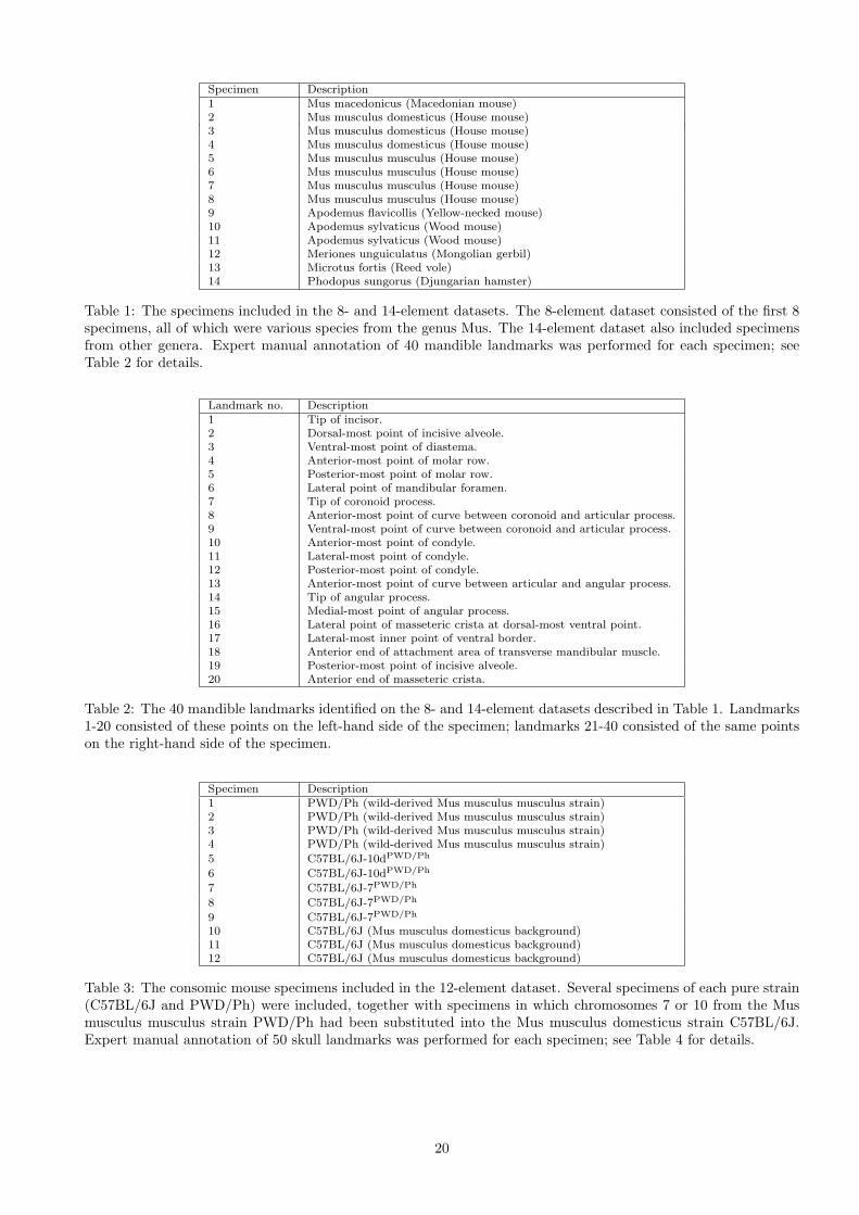
Table 1: The specimens included in the 8- and 14-element datasets. The 8-element dataset consisted of the first 8specimens, all of which were various species from the genus Mus. The 14-element dataset also included specimensfrom other genera. Expert manual annotation of 40 mandible landmarks was performed for each specimen; seeTable 2 for details.

Landmark no. Description1 Tip of incisor.2 Dorsal-most point of incisive alveole.3 Ventral-most point of diastema.4 Anterior-most point of molar row.5 Posterior-most point of molar row.6 Lateral point of mandibular foramen.7 Tip of coronoid process.8 Anterior-most point of curve between coronoid and articular process.9 Ventral-most point of curve between coronoid and articular process.10 Anterior-most point of condyle.11 Lateral-most point of condyle.12 Posterior-most point of condyle.13 Anterior-most point of curve between articular and angular process.14 Tip of angular process.15 Medial-most point of angular process.16 Lateral point of masseteric crista at dorsal-most ventral point.17 Lateral-most inner point of ventral border.18 Anterior end of attachment area of transverse mandibular muscle.19 Posterior-most point of incisive alveole.20 Anterior end of masseteric crista.

Table 2: The 40 mandible landmarks identified on the 8- and 14-element datasets described in Table 1. Landmarks1-20 consisted of these points on the left-hand side of the specimen; landmarks 21-40 consisted of the same pointson the right-hand side of the specimen.

Specimen Description1 PWD/Ph (wild-derived Mus musculus musculus strain)2 PWD/Ph (wild-derived Mus musculus musculus strain)3 PWD/Ph (wild-derived Mus musculus musculus strain)4 PWD/Ph (wild-derived Mus musculus musculus strain)

5 C57BL/6J-10dPWD/Ph

6 C57BL/6J-10dPWD/Ph

7 C57BL/6J-7PWD/Ph

8 C57BL/6J-7PWD/Ph

9 C57BL/6J-7PWD/Ph

10 C57BL/6J (Mus musculus domesticus background)11 C57BL/6J (Mus musculus domesticus background)12 C57BL/6J (Mus musculus domesticus background)

Table 3: The consomic mouse specimens included in the 12-element dataset. Several specimens of each pure strain(C57BL/6J and PWD/Ph) were included, together with specimens in which chromosomes 7 or 10 from the Musmusculus musculus strain PWD/Ph had been substituted into the Mus musculus domesticus strain C57BL/6J.Expert manual annotation of 50 skull landmarks was performed for each specimen; see Table 4 for details.

20

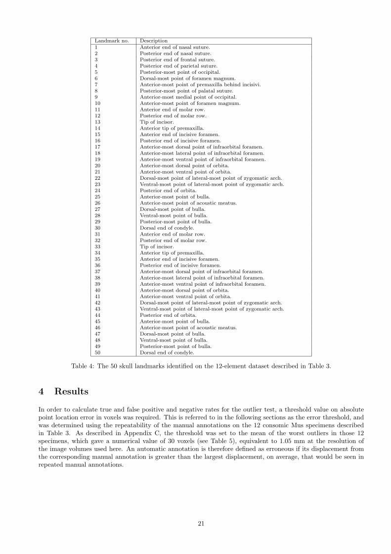
Landmark no. Description1 Anterior end of nasal suture.2 Posterior end of nasal suture.3 Posterior end of frontal suture.4 Posterior end of parietal suture.5 Posterior-most point of occipital.6 Dorsal-most point of foramen magnum.7 Anterior-most point of premaxilla behind incisivi.8 Posterior-most point of palatal suture.9 Anterior-most medial point of occipital.10 Anterior-most point of foramen magnum.11 Anterior end of molar row.12 Posterior end of molar row.13 Tip of incisor.14 Anterior tip of premaxilla.15 Anterior end of incisive foramen.16 Posterior end of incisive foramen.17 Anterior-most dorsal point of infraorbital foramen.18 Anterior-most lateral point of infraorbital foramen.19 Anterior-most ventral point of infraorbital foramen.20 Anterior-most dorsal point of orbita.21 Anterior-most ventral point of orbita.22 Dorsal-most point of lateral-most point of zygomatic arch.23 Ventral-most point of lateral-most point of zygomatic arch.24 Posterior end of orbita.25 Anterior-most point of bulla.26 Anterior-most point of acoustic meatus.27 Dorsal-most point of bulla.28 Ventral-most point of bulla.29 Posterior-most point of bulla.30 Dorsal end of condyle.31 Anterior end of molar row.32 Posterior end of molar row.33 Tip of incisor.34 Anterior tip of premaxilla.35 Anterior end of incisive foramen.36 Posterior end of incisive foramen.37 Anterior-most dorsal point of infraorbital foramen.38 Anterior-most lateral point of infraorbital foramen.39 Anterior-most ventral point of infraorbital foramen.40 Anterior-most dorsal point of orbita.41 Anterior-most ventral point of orbita.42 Dorsal-most point of lateral-most point of zygomatic arch.43 Ventral-most point of lateral-most point of zygomatic arch.44 Posterior end of orbita.45 Anterior-most point of bulla.46 Anterior-most point of acoustic meatus.47 Dorsal-most point of bulla.48 Ventral-most point of bulla.49 Posterior-most point of bulla.50 Dorsal end of condyle.

Table 4: The 50 skull landmarks identified on the 12-element dataset described in Table 3.

4 Results

In order to calculate true and false positive and negative rates for the outlier test, a threshold value on absolutepoint location error in voxels was required. This is referred to in the following sections as the error threshold, andwas determined using the repeatability of the manual annotations on the 12 consomic Mus specimens describedin Table 3. As described in Appendix C, the threshold was set to the mean of the worst outliers in those 12specimens, which gave a numerical value of 30 voxels (see Table 5), equivalent to 1.05 mm at the resolution ofthe image volumes used here. An automatic annotation is therefore defined as erroneous if its displacement fromthe corresponding manual annotation is greater than the largest displacement, on average, that would be seen inrepeated manual annotations.

21

Experiment. M1 (voxels) M2 (voxels) O1 (voxels) O2 (voxels) % passing % withinthreshold

12 Mus, SP, LM 1 3.66 ± 1.54 4.93 ± 4.47 18.11 ± 5.49 23.15 ± 13.08 87.0 ± 7.1 98.5 ± 1.512 Mus, SP, LM 2 3.60 ± 1.38 4.58 ± 3.63 20.42 ± 6.12 19.52 ± 6.25 87.5 ± 9.6 98.3 ± 2.112 Mus, DP 1st iter., LM 1 3.99 ± 1.81 5.16 ± 3.93 17.31 ± 2.52 17.87 ± 6.12 72.0 ± 21.4 96.3 ± 3.312 Mus, DP 2nd iter., LM 1 3.79 ± 1.61 4.82 ± 4.36 16.14 ± 2.28 22.53 ± 13.33 86.2 ± 6.7 97.7 ± 2.112 Mus, DP 1st iter., LM 2 3.85 ± 1.56 4.84 ± 3.77 17.57 ± 3.38 18.25 ± 5.88 69.8 ± 21.0 96.7 ± 2.112 Mus, DP 2nd iter., LM 2 3.49 ± 1.38 4.35 ± 3.27 13.69 ± 2.03 16.88 ± 7.12 87.3 ± 7.6 97.8 ± 2.0Manual repeatability 3.34 ± 1.43 4.53 ± 4.89 28.76 ± 5.98 29.33 ± 12.23 - -12 Mus, SP repeatability 1.41 ± 0.59 2.09 ± 1.64 7.03 ± 1.43 7.43 ± 2.28 81.8 ± 9.6 -12 Mus, DP repeatability 2.00 ± 0.59 2.22 ± 1.59 7.71 ± 1.46 7.93 ± 2.39 81.5 ± 8.9 -14 rodents 5.11 ± 2.43 6.91 ± 5.71 22.90 ± 2.03 23.09 ± 6.06 41.4 ± 25.3 82.7 ± 22.514 rodents, Mus only 5.11 ± 2.29 6.69 ± 5.14 22.03 ± 3.92 22.18 ± 6.63 57.8 ± 10.7 95.0 ± 4.814 rodents, Apodemus only 6.83 ± 3.51 9.12 ± 7.11 24.20 ± 2.06 25.52 ± 4.20 38.3 ± 10.4 90.0 ± 4.314 rodents, others - - - - 0.0 42.5 ± 9.08 Mus from 14 rodent set 5.24 ± 2.37 6.78 ± 5.03 21.04 ± 4.88 22.35 ± 6.78 73.8 ± 12.7 95.3 ± 5.3

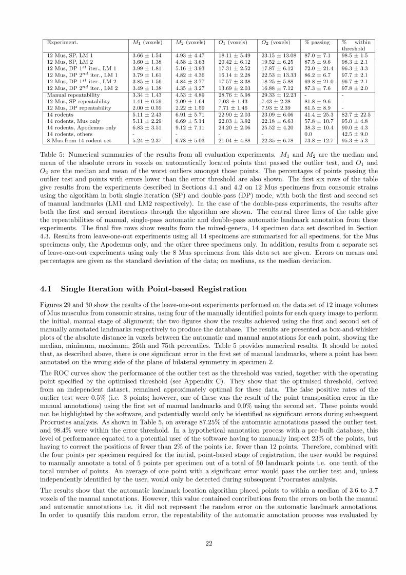
Table 5: Numerical summaries of the results from all evaluation experiments. M1 and M2 are the median andmean of the absolute errors in voxels on automatically located points that passed the outlier test, and O1 andO2 are the median and mean of the worst outliers amongst those points. The percentages of points passing theoutlier test and points with errors lower than the error threshold are also shown. The first six rows of the tablegive results from the experiments described in Sections 4.1 and 4.2 on 12 Mus specimens from consomic strainsusing the algorithm in both single-iteration (SP) and double-pass (DP) mode, with both the first and second setof manual landmarks (LM1 and LM2 respectively). In the case of the double-pass experiments, the results afterboth the first and second iterations through the algorithm are shown. The central three lines of the table givethe repeatabilities of manual, single-pass automatic and double-pass automatic landmark annotation from theseexperiments. The final five rows show results from the mixed-genera, 14 specimen data set described in Section4.3. Results from leave-one-out experiments using all 14 specimens are summarised for all specimens, for the Musspecimens only, the Apodemus only, and the other three specimens only. In addition, results from a separate setof leave-one-out experiments using only the 8 Mus specimens from this data set are given. Errors on means andpercentages are given as the standard deviation of the data; on medians, as the median deviation.

4.1 Single Iteration with Point-based Registration

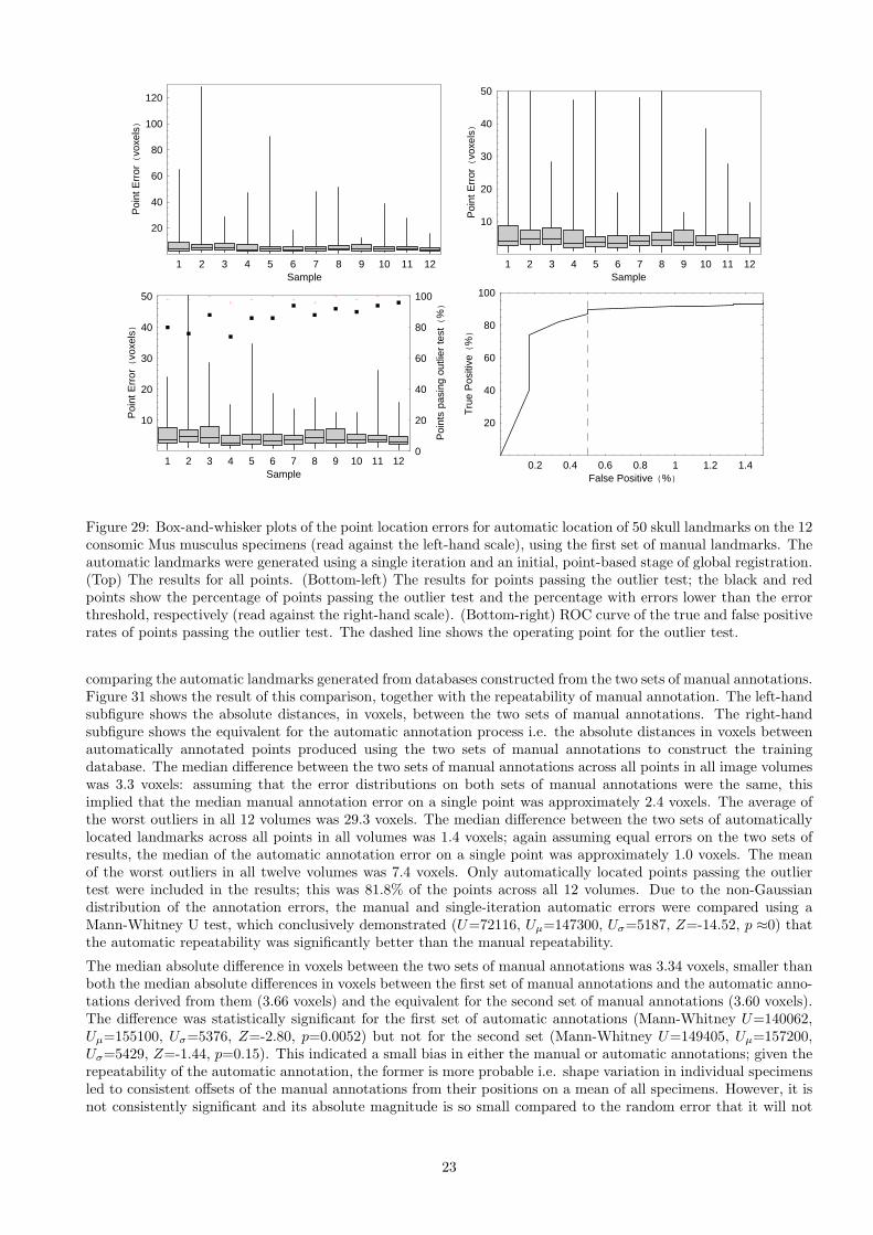
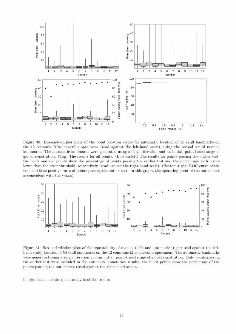
Figures 29 and 30 show the results of the leave-one-out experiments performed on the data set of 12 image volumesof Mus musculus from consomic strains, using four of the manually identified points for each query image to performthe initial, manual stage of alignment; the two figures show the results achieved using the first and second set ofmanually annotated landmarks respectively to produce the database. The results are presented as box-and-whiskerplots of the absolute distance in voxels between the automatic and manual annotations for each point, showing themedian, minimum, maximum, 25th and 75th percentiles. Table 5 provides numerical results. It should be notedthat, as described above, there is one significant error in the first set of manual landmarks, where a point has beenannotated on the wrong side of the plane of bilateral symmetry in specimen 2.

The ROC curves show the performance of the outlier test as the threshold was varied, together with the operatingpoint specified by the optimised threshold (see Appendix C). They show that the optimised threshold, derivedfrom an independent dataset, remained approximately optimal for these data. The false positive rates of theoutlier test were 0.5% (i.e. 3 points; however, one of these was the result of the point transposition error in themanual annotations) using the first set of manual landmarks and 0.0% using the second set. These points wouldnot be highlighted by the software, and potentially would only be identified as significant errors during subsequentProcrustes analysis. As shown in Table 5, on average 87.25% of the automatic annotations passed the outlier test,and 98.4% were within the error threshold. In a hypothetical annotation process with a pre-built database, thislevel of performance equated to a potential user of the software having to manually inspect 23% of the points, buthaving to correct the positions of fewer than 2% of the points i.e. fewer than 12 points. Therefore, combined withthe four points per specimen required for the initial, point-based stage of registration, the user would be requiredto manually annotate a total of 5 points per specimen out of a total of 50 landmark points i.e. one tenth of thetotal number of points. An average of one point with a significant error would pass the outlier test and, unlessindependently identified by the user, would only be detected during subsequent Procrustes analysis.

The results show that the automatic landmark location algorithm placed points to within a median of 3.6 to 3.7voxels of the manual annotations. However, this value contained contributions from the errors on both the manualand automatic annotations i.e. it did not represent the random error on the automatic landmark annotations.In order to quantify this random error, the repeatability of the automatic annotation process was evaluated by

22

1 2 3 4 5 6 7 8 9 10 11 12Sample

20

40

60

80

100

120

Poi

ntE

rror(

voxe

ls)

1 2 3 4 5 6 7 8 9 10 11 12Sample

10

20

30

40

50

Poi

ntE

rror(

voxe

ls)

1 2 3 4 5 6 7 8 9 10 11 12Sample

10

20

30

40

50

Poi

ntE

rror(

voxe

ls)

0

20

40

60

80

100

Poi

nts

pasi

ngou

tlier

test(

%)

0.2 0.4 0.6 0.8 1 1.2 1.4False Positive (%)

20

40

60

80

100

Tru

eP

ositi

ve(

%)

Figure 29: Box-and-whisker plots of the point location errors for automatic location of 50 skull landmarks on the 12consomic Mus musculus specimens (read against the left-hand scale), using the first set of manual landmarks. Theautomatic landmarks were generated using a single iteration and an initial, point-based stage of global registration.(Top) The results for all points. (Bottom-left) The results for points passing the outlier test; the black and redpoints show the percentage of points passing the outlier test and the percentage with errors lower than the errorthreshold, respectively (read against the right-hand scale). (Bottom-right) ROC curve of the true and false positiverates of points passing the outlier test. The dashed line shows the operating point for the outlier test.

comparing the automatic landmarks generated from databases constructed from the two sets of manual annotations.Figure 31 shows the result of this comparison, together with the repeatability of manual annotation. The left-handsubfigure shows the absolute distances, in voxels, between the two sets of manual annotations. The right-handsubfigure shows the equivalent for the automatic annotation process i.e. the absolute distances in voxels betweenautomatically annotated points produced using the two sets of manual annotations to construct the trainingdatabase. The median difference between the two sets of manual annotations across all points in all image volumeswas 3.3 voxels: assuming that the error distributions on both sets of manual annotations were the same, thisimplied that the median manual annotation error on a single point was approximately 2.4 voxels. The average ofthe worst outliers in all 12 volumes was 29.3 voxels. The median difference between the two sets of automaticallylocated landmarks across all points in all volumes was 1.4 voxels; again assuming equal errors on the two sets ofresults, the median of the automatic annotation error on a single point was approximately 1.0 voxels. The meanof the worst outliers in all twelve volumes was 7.4 voxels. Only automatically located points passing the outliertest were included in the results; this was 81.8% of the points across all 12 volumes. Due to the non-Gaussiandistribution of the annotation errors, the manual and single-iteration automatic errors were compared using aMann-Whitney U test, which conclusively demonstrated (U=72116, Uµ=147300, Uσ=5187, Z=-14.52, p ≈0) thatthe automatic repeatability was significantly better than the manual repeatability.

The median absolute difference in voxels between the two sets of manual annotations was 3.34 voxels, smaller thanboth the median absolute differences in voxels between the first set of manual annotations and the automatic anno-tations derived from them (3.66 voxels) and the equivalent for the second set of manual annotations (3.60 voxels).The difference was statistically significant for the first set of automatic annotations (Mann-Whitney U=140062,Uµ=155100, Uσ=5376, Z=-2.80, p=0.0052) but not for the second set (Mann-Whitney U=149405, Uµ=157200,Uσ=5429, Z=-1.44, p=0.15). This indicated a small bias in either the manual or automatic annotations; given therepeatability of the automatic annotation, the former is more probable i.e. shape variation in individual specimensled to consistent offsets of the manual annotations from their positions on a mean of all specimens. However, it isnot consistently significant and its absolute magnitude is so small compared to the random error that it will not

23

1 2 3 4 5 6 7 8 9 10 11 12Sample

20

40

60

80

100

Poi

ntE

rror(

voxe

ls)

1 2 3 4 5 6 7 8 9 10 11 12Sample

10

20

30

40

50

Poi

ntE

rror(

voxe

ls)

1 2 3 4 5 6 7 8 9 10 11 12Sample

10

20

30

40

50

Poi

ntE

rror(

voxe

ls)

0

20

40

60

80

100

Poi

nts

pasi

ngou

tlier

test(

%)

0.2 0.4 0.6 0.8 1 1.2 1.4False Positive (%)

20

40

60

80

100

Tru

eP

ositi

ve(

%)

Figure 30: Box-and-whisker plots of the point location errors for automatic location of 50 skull landmarks onthe 12 consomic Mus musculus specimens (read against the left-hand scale), using the second set of manuallandmarks. The automatic landmarks were generated using a single iteration and an initial, point-based stage ofglobal registration. (Top) The results for all points. (Bottom-left) The results for points passing the outlier test;the black and red points show the percentage of points passing the outlier test and the percentage with errorslower than the error threshold, respectively (read against the right-hand scale). (Bottom-right) ROC curve of thetrue and false positive rates of points passing the outlier test. In this graph, the operating point of the outlier testis coincident with the y-axis).

1 2 3 4 5 6 7 8 9 10 11 12Sample

10

20

30

40

50

Poi

ntE

rror(

voxe

ls)

1 2 3 4 5 6 7 8 9 10 11 12Sample

10

20

30

40

50

Poi

ntE

rror(

voxe

ls)

0

20

40

60

80

100

Poi

nts

pass

ing

outli

erte

st(

%)

Figure 31: Box-and-whisker plots of the repeatability of manual (left) and automatic (right; read against the left-hand scale) location of 50 skull landmarks on the 12 consomic Mus musculus specimens. The automatic landmarkswere generated using a single iteration and an initial, point-based stage of global registration. Only points passingthe outlier test were included in the automatic annotation results; the black points show the percentage of thepoints passing the outlier test (read against the right-hand scale).

be significant in subsequent analysis of the results.

24

1 2 3 4 5 6 7 8 9 10 11 12Sample

50

100

150

200

250

300

350

Poi

ntE

rror(

voxe

ls)

1 2 3 4 5 6 7 8 9 10 11 12Sample

10

20

30

40

50

Poi

ntE

rror(

voxe

ls)

1 2 3 4 5 6 7 8 9 10 11 12Sample

10

20

30

40

50

Poi

ntE

rror(

voxe

ls)

0

20

40

60

80

100

Poi

nts

pasi

ngou

tlier

test(

%)

0.5 1 1.5 2 2.5False Positive (%)

20

40

60

80

100

Tru

eP

ositi

ve(

%)

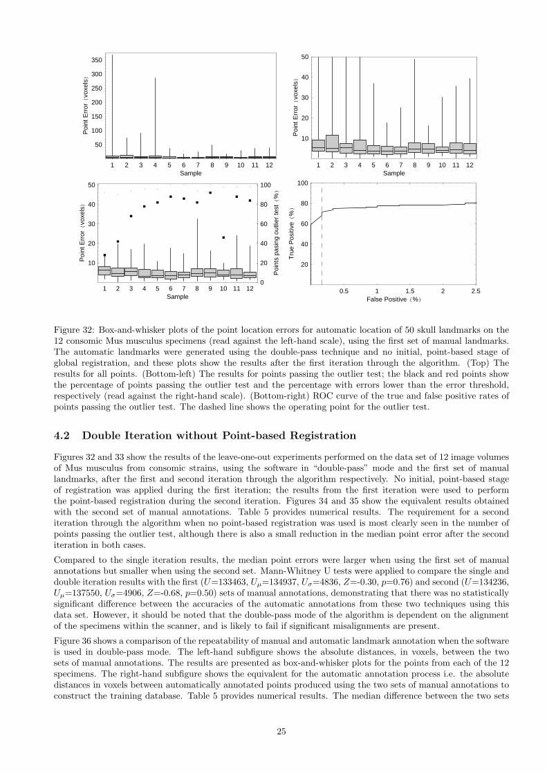
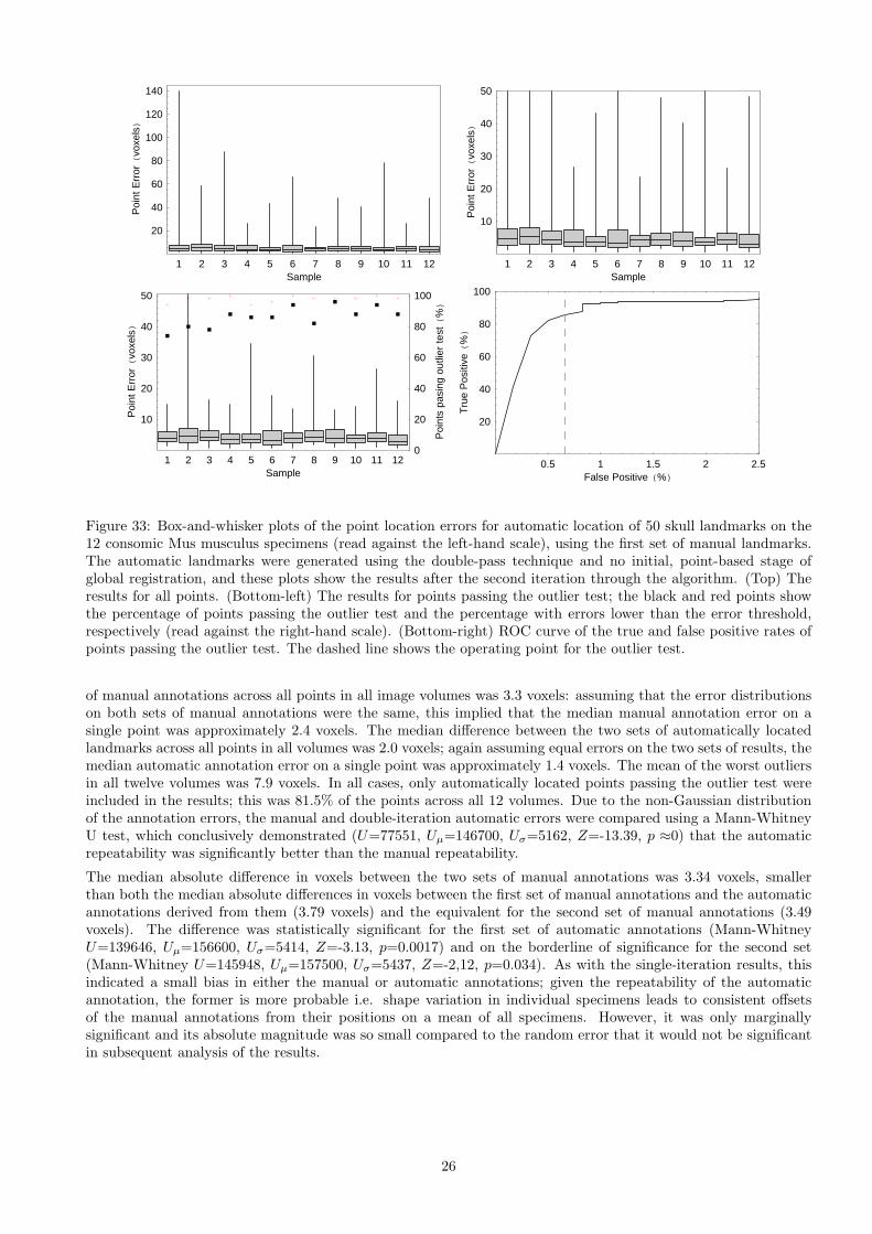
Figure 32: Box-and-whisker plots of the point location errors for automatic location of 50 skull landmarks on the12 consomic Mus musculus specimens (read against the left-hand scale), using the first set of manual landmarks.The automatic landmarks were generated using the double-pass technique and no initial, point-based stage ofglobal registration, and these plots show the results after the first iteration through the algorithm. (Top) Theresults for all points. (Bottom-left) The results for points passing the outlier test; the black and red points showthe percentage of points passing the outlier test and the percentage with errors lower than the error threshold,respectively (read against the right-hand scale). (Bottom-right) ROC curve of the true and false positive rates ofpoints passing the outlier test. The dashed line shows the operating point for the outlier test.

4.2 Double Iteration without Point-based Registration

Figures 32 and 33 show the results of the leave-one-out experiments performed on the data set of 12 image volumesof Mus musculus from consomic strains, using the software in “double-pass” mode and the first set of manuallandmarks, after the first and second iteration through the algorithm respectively. No initial, point-based stageof registration was applied during the first iteration; the results from the first iteration were used to performthe point-based registration during the second iteration. Figures 34 and 35 show the equivalent results obtainedwith the second set of manual annotations. Table 5 provides numerical results. The requirement for a seconditeration through the algorithm when no point-based registration was used is most clearly seen in the number ofpoints passing the outlier test, although there is also a small reduction in the median point error after the seconditeration in both cases.

Compared to the single iteration results, the median point errors were larger when using the first set of manualannotations but smaller when using the second set. Mann-Whitney U tests were applied to compare the single anddouble iteration results with the first (U=133463, Uµ=134937, Uσ=4836, Z=-0.30, p=0.76) and second (U=134236,Uµ=137550, Uσ=4906, Z=-0.68, p=0.50) sets of manual annotations, demonstrating that there was no statisticallysignificant difference between the accuracies of the automatic annotations from these two techniques using thisdata set. However, it should be noted that the double-pass mode of the algorithm is dependent on the alignmentof the specimens within the scanner, and is likely to fail if significant misalignments are present.

Figure 36 shows a comparison of the repeatability of manual and automatic landmark annotation when the softwareis used in double-pass mode. The left-hand subfigure shows the absolute distances, in voxels, between the twosets of manual annotations. The results are presented as box-and-whisker plots for the points from each of the 12specimens. The right-hand subfigure shows the equivalent for the automatic annotation process i.e. the absolutedistances in voxels between automatically annotated points produced using the two sets of manual annotations toconstruct the training database. Table 5 provides numerical results. The median difference between the two sets

25

1 2 3 4 5 6 7 8 9 10 11 12Sample

20

40

60

80

100

120

140

Poi

ntE

rror(

voxe

ls)

1 2 3 4 5 6 7 8 9 10 11 12Sample

10

20

30

40

50

Poi

ntE

rror(

voxe

ls)

1 2 3 4 5 6 7 8 9 10 11 12Sample

10

20

30

40

50

Poi

ntE

rror(

voxe

ls)

0

20

40

60

80

100

Poi

nts

pasi

ngou

tlier

test(

%)

0.5 1 1.5 2 2.5False Positive (%)

20

40

60

80

100

Tru

eP

ositi

ve(

%)

Figure 33: Box-and-whisker plots of the point location errors for automatic location of 50 skull landmarks on the12 consomic Mus musculus specimens (read against the left-hand scale), using the first set of manual landmarks.The automatic landmarks were generated using the double-pass technique and no initial, point-based stage ofglobal registration, and these plots show the results after the second iteration through the algorithm. (Top) Theresults for all points. (Bottom-left) The results for points passing the outlier test; the black and red points showthe percentage of points passing the outlier test and the percentage with errors lower than the error threshold,respectively (read against the right-hand scale). (Bottom-right) ROC curve of the true and false positive rates ofpoints passing the outlier test. The dashed line shows the operating point for the outlier test.

of manual annotations across all points in all image volumes was 3.3 voxels: assuming that the error distributionson both sets of manual annotations were the same, this implied that the median manual annotation error on asingle point was approximately 2.4 voxels. The median difference between the two sets of automatically locatedlandmarks across all points in all volumes was 2.0 voxels; again assuming equal errors on the two sets of results, themedian automatic annotation error on a single point was approximately 1.4 voxels. The mean of the worst outliersin all twelve volumes was 7.9 voxels. In all cases, only automatically located points passing the outlier test wereincluded in the results; this was 81.5% of the points across all 12 volumes. Due to the non-Gaussian distributionof the annotation errors, the manual and double-iteration automatic errors were compared using a Mann-WhitneyU test, which conclusively demonstrated (U=77551, Uµ=146700, Uσ=5162, Z=-13.39, p ≈0) that the automaticrepeatability was significantly better than the manual repeatability.

The median absolute difference in voxels between the two sets of manual annotations was 3.34 voxels, smallerthan both the median absolute differences in voxels between the first set of manual annotations and the automaticannotations derived from them (3.79 voxels) and the equivalent for the second set of manual annotations (3.49voxels). The difference was statistically significant for the first set of automatic annotations (Mann-WhitneyU=139646, Uµ=156600, Uσ=5414, Z=-3.13, p=0.0017) and on the borderline of significance for the second set(Mann-Whitney U=145948, Uµ=157500, Uσ=5437, Z=-2,12, p=0.034). As with the single-iteration results, thisindicated a small bias in either the manual or automatic annotations; given the repeatability of the automaticannotation, the former is more probable i.e. shape variation in individual specimens leads to consistent offsetsof the manual annotations from their positions on a mean of all specimens. However, it was only marginallysignificant and its absolute magnitude was so small compared to the random error that it would not be significantin subsequent analysis of the results.

26

1 2 3 4 5 6 7 8 9 10 11 12Sample

50

100

150

200

250

300

350

Poi

ntE

rror(

voxe

lsL

1 2 3 4 5 6 7 8 9 10 11 12Sample

10

20

30

40

50

Poi

ntE

rror(

voxe

lsL

1 2 3 4 5 6 7 8 9 10 11 12Sample

10

20

30

40

50

Poi

ntE

rror(

voxe

lsL

0

20

40

60

80

100

Poi

nts

pasi

ngou

tlier

test(

%L

0.5 1 1.5 2 2.5False Positive (%L

20

40

60

80

100

Tru

eP

ositi

ve(

%L

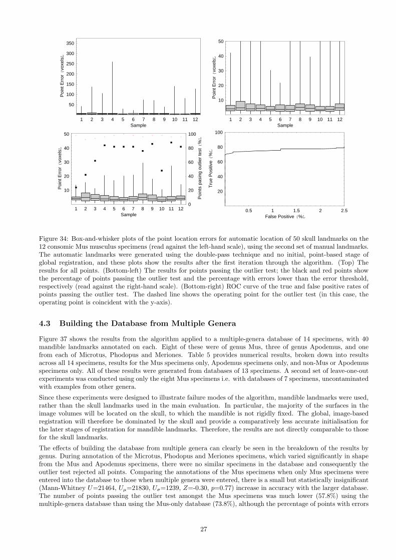
Figure 34: Box-and-whisker plots of the point location errors for automatic location of 50 skull landmarks on the12 consomic Mus musculus specimens (read against the left-hand scale), using the second set of manual landmarks.The automatic landmarks were generated using the double-pass technique and no initial, point-based stage ofglobal registration, and these plots show the results after the first iteration through the algorithm. (Top) Theresults for all points. (Bottom-left) The results for points passing the outlier test; the black and red points showthe percentage of points passing the outlier test and the percentage with errors lower than the error threshold,respectively (read against the right-hand scale). (Bottom-right) ROC curve of the true and false positive rates ofpoints passing the outlier test. The dashed line shows the operating point for the outlier test (in this case, theoperating point is coincident with the y-axis).

4.3 Building the Database from Multiple Genera

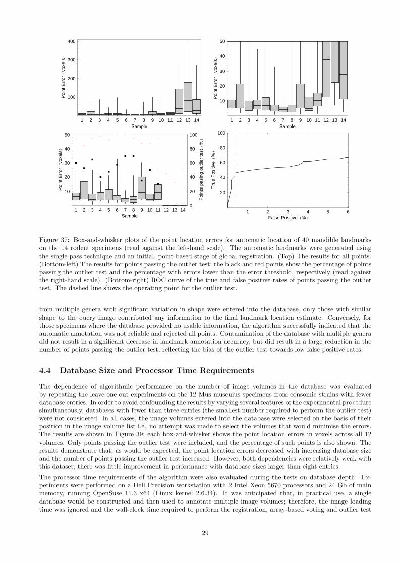
Figure 37 shows the results from the algorithm applied to a multiple-genera database of 14 specimens, with 40mandible landmarks annotated on each. Eight of these were of genus Mus, three of genus Apodemus, and onefrom each of Microtus, Phodopus and Meriones. Table 5 provides numerical results, broken down into resultsacross all 14 specimens, results for the Mus specimens only, Apodemus specimens only, and non-Mus or Apodemusspecimens only. All of these results were generated from databases of 13 specimens. A second set of leave-one-outexperiments was conducted using only the eight Mus specimens i.e. with databases of 7 specimens, uncontaminatedwith examples from other genera.

Since these experiments were designed to illustrate failure modes of the algorithm, mandible landmarks were used,rather than the skull landmarks used in the main evaluation. In particular, the majority of the surfaces in theimage volumes will be located on the skull, to which the mandible is not rigidly fixed. The global, image-basedregistration will therefore be dominated by the skull and provide a comparatively less accurate initialisation forthe later stages of registration for mandible landmarks. Therefore, the results are not directly comparable to thosefor the skull landmarks.

The effects of building the database from multiple genera can clearly be seen in the breakdown of the results bygenus. During annotation of the Microtus, Phodopus and Meriones specimens, which varied significantly in shapefrom the Mus and Apodemus specimens, there were no similar specimens in the database and consequently theoutlier test rejected all points. Comparing the annotations of the Mus specimens when only Mus specimens wereentered into the database to those when multiple genera were entered, there is a small but statistically insignificant(Mann-Whitney U=21464, Uµ=21830, Uσ=1239, Z=-0.30, p=0.77) increase in accuracy with the larger database.The number of points passing the outlier test amongst the Mus specimens was much lower (57.8%) using themultiple-genera database than using the Mus-only database (73.8%), although the percentage of points with errors

27

1 2 3 4 5 6 7 8 9 10 11 12Sample

20

40

60

80

100

120

Poi

ntE

rror(

voxe

ls)

1 2 3 4 5 6 7 8 9 10 11 12Sample

10

20

30

40

50

Poi

ntE

rror(

voxe

ls)

1 2 3 4 5 6 7 8 9 10 11 12Sample

10

20

30

40

50

Poi

ntE

rror(

voxe

ls)

0

20

40

60

80

100

Poi

nts

pasi

ngou

tlier

test(

%)

0.25 0.5 0.75 1 1.25 1.5 1.75 2False Positive (%)

20

40

60

80

100

Tru

eP

ositi

ve(

%)

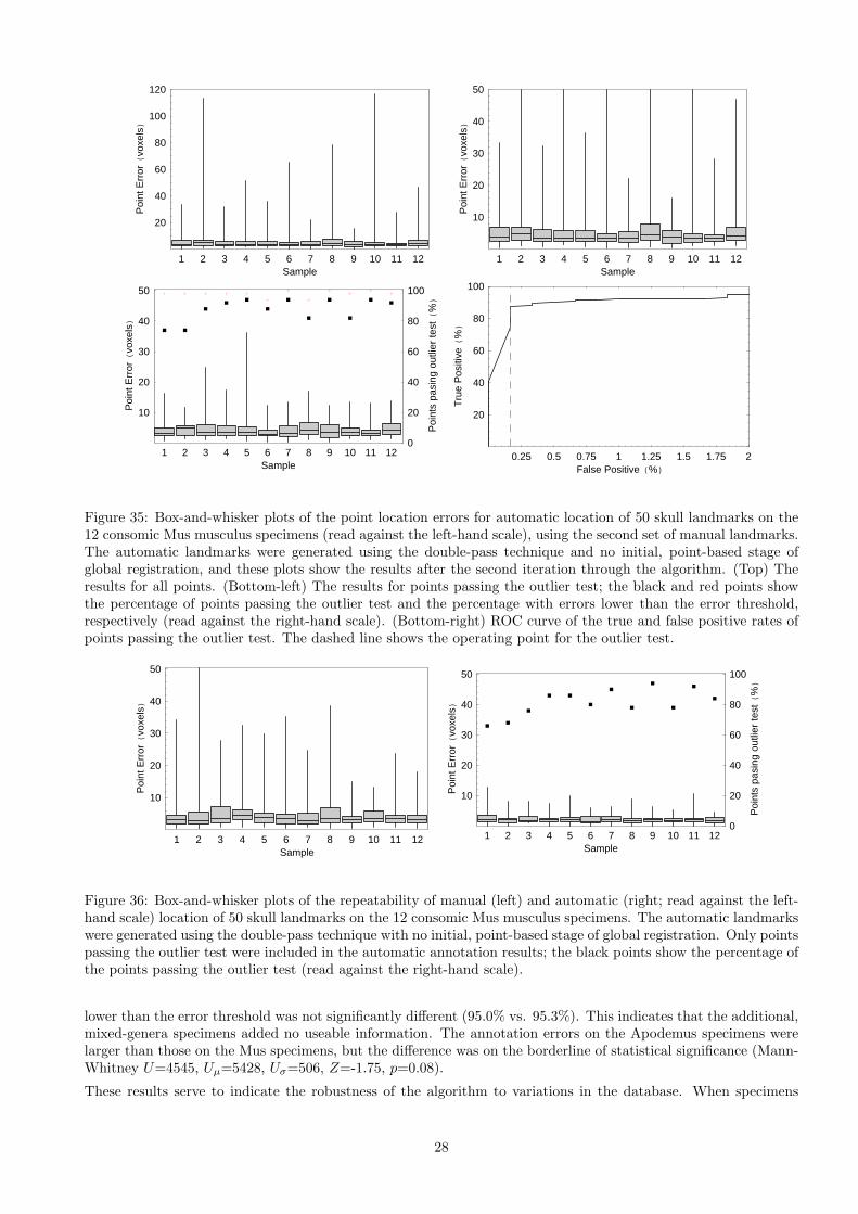
Figure 35: Box-and-whisker plots of the point location errors for automatic location of 50 skull landmarks on the12 consomic Mus musculus specimens (read against the left-hand scale), using the second set of manual landmarks.The automatic landmarks were generated using the double-pass technique and no initial, point-based stage ofglobal registration, and these plots show the results after the second iteration through the algorithm. (Top) Theresults for all points. (Bottom-left) The results for points passing the outlier test; the black and red points showthe percentage of points passing the outlier test and the percentage with errors lower than the error threshold,respectively (read against the right-hand scale). (Bottom-right) ROC curve of the true and false positive rates ofpoints passing the outlier test. The dashed line shows the operating point for the outlier test.

1 2 3 4 5 6 7 8 9 10 11 12Sample

10

20

30

40

50

Poi

ntE

rror(

voxe

ls)

1 2 3 4 5 6 7 8 9 10 11 12Sample

10

20

30

40

50

Poi

ntE

rror(

voxe

ls)

0

20

40

60

80

100

Poi

nts

pasi

ngou

tlier

test(

%)

Figure 36: Box-and-whisker plots of the repeatability of manual (left) and automatic (right; read against the left-hand scale) location of 50 skull landmarks on the 12 consomic Mus musculus specimens. The automatic landmarkswere generated using the double-pass technique with no initial, point-based stage of global registration. Only pointspassing the outlier test were included in the automatic annotation results; the black points show the percentage ofthe points passing the outlier test (read against the right-hand scale).

lower than the error threshold was not significantly different (95.0% vs. 95.3%). This indicates that the additional,mixed-genera specimens added no useable information. The annotation errors on the Apodemus specimens werelarger than those on the Mus specimens, but the difference was on the borderline of statistical significance (Mann-Whitney U=4545, Uµ=5428, Uσ=506, Z=-1.75, p=0.08).

These results serve to indicate the robustness of the algorithm to variations in the database. When specimens

28

1 2 3 4 5 6 7 8 9 10 11 12 13 14Sample

100

200

300

400

Poi

ntE

rror(

voxe

ls)

1 2 3 4 5 6 7 8 9 10 11 12 13 14Sample

10

20

30

40

50

Poi

ntE

rror(

voxe

ls)

1 2 3 4 5 6 7 8 9 10 11 12 13 14Sample

10

20

30

40

50

Poi

ntE

rror(

voxe

ls)

0

20

40

60

80

100

Poi

nts

pasi

ngou

tlier

test(

%)

1 2 3 4 5 6False Positive (%)

20

40

60

80

100

Tru

eP

ositi

ve(

%)

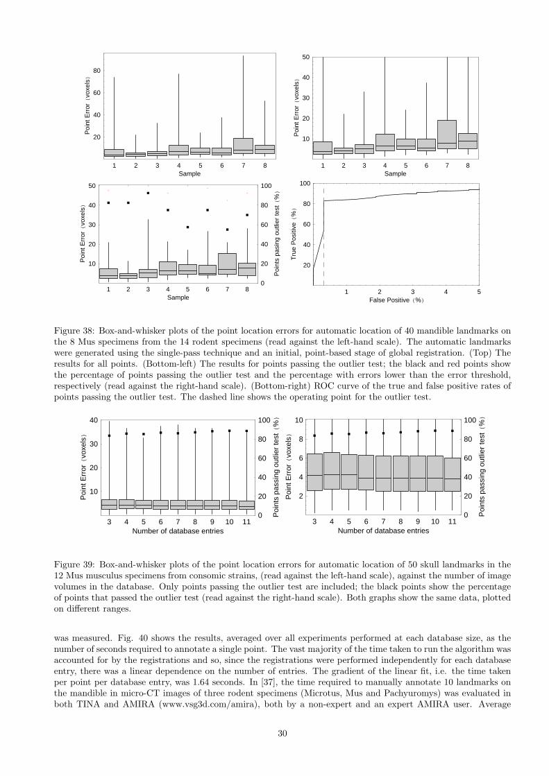
Figure 37: Box-and-whisker plots of the point location errors for automatic location of 40 mandible landmarkson the 14 rodent specimens (read against the left-hand scale). The automatic landmarks were generated usingthe single-pass technique and an initial, point-based stage of global registration. (Top) The results for all points.(Bottom-left) The results for points passing the outlier test; the black and red points show the percentage of pointspassing the outlier test and the percentage with errors lower than the error threshold, respectively (read againstthe right-hand scale). (Bottom-right) ROC curve of the true and false positive rates of points passing the outliertest. The dashed line shows the operating point for the outlier test.

from multiple genera with significant variation in shape were entered into the database, only those with similarshape to the query image contributed any information to the final landmark location estimate. Conversely, forthose specimens where the database provided no usable information, the algorithm successfully indicated that theautomatic annotation was not reliable and rejected all points. Contamination of the database with multiple generadid not result in a significant decrease in landmark annotation accuracy, but did result in a large reduction in thenumber of points passing the outlier test, reflecting the bias of the outlier test towards low false positive rates.

4.4 Database Size and Processor Time Requirements

The dependence of algorithmic performance on the number of image volumes in the database was evaluatedby repeating the leave-one-out experiments on the 12 Mus musculus specimens from consomic strains with fewerdatabase entries. In order to avoid confounding the results by varying several features of the experimental proceduresimultaneously, databases with fewer than three entries (the smallest number required to perform the outlier test)were not considered. In all cases, the image volumes entered into the database were selected on the basis of theirposition in the image volume list i.e. no attempt was made to select the volumes that would minimise the errors.The results are shown in Figure 39; each box-and-whisker shows the point location errors in voxels across all 12volumes. Only points passing the outlier test were included, and the percentage of such points is also shown. Theresults demonstrate that, as would be expected, the point location errors decreased with increasing database sizeand the number of points passing the outlier test increased. However, both dependencies were relatively weak withthis dataset; there was little improvement in performance with database sizes larger than eight entries.

The processor time requirements of the algorithm were also evaluated during the tests on database depth. Ex-periments were performed on a Dell Precision workstation with 2 Intel Xeon 5670 processors and 24 Gb of mainmemory, running OpenSuse 11.3 x64 (Linux kernel 2.6.34). It was anticipated that, in practical use, a singledatabase would be constructed and then used to annotate multiple image volumes; therefore, the image loadingtime was ignored and the wall-clock time required to perform the registration, array-based voting and outlier test

29

1 2 3 4 5 6 7 8Sample

20

40

60

80

Poi

ntE

rror(

voxe

ls)

1 2 3 4 5 6 7 8Sample

10

20

30

40

50

Poi

ntE

rror(

voxe

ls)

1 2 3 4 5 6 7 8Sample

10

20

30

40

50

Poi

ntE

rror(

voxe

ls)

0

20

40

60

80

100

Poi

nts

pasi

ngou

tlier

test(

%)

1 2 3 4 5False Positive (%)

20

40

60

80

100

Tru

eP

ositi

ve(

%)

Figure 38: Box-and-whisker plots of the point location errors for automatic location of 40 mandible landmarks onthe 8 Mus specimens from the 14 rodent specimens (read against the left-hand scale). The automatic landmarkswere generated using the single-pass technique and an initial, point-based stage of global registration. (Top) Theresults for all points. (Bottom-left) The results for points passing the outlier test; the black and red points showthe percentage of points passing the outlier test and the percentage with errors lower than the error threshold,respectively (read against the right-hand scale). (Bottom-right) ROC curve of the true and false positive rates ofpoints passing the outlier test. The dashed line shows the operating point for the outlier test.

3 4 5 6 7 8 9 10 11Number of database entries

10

20

30

40

Poi

ntE

rror(

voxe

ls)

0

20

40

60

80

100

Poi

nts

pass

ing

outli

erte

st(

%)

3 4 5 6 7 8 9 10 11Number of database entries

2

4

6

8

10

Poi

ntE

rror(

voxe

ls)

0

20

40

60

80

100

Poi

nts

pass

ing

outli

erte

st(

%)

Figure 39: Box-and-whisker plots of the point location errors for automatic location of 50 skull landmarks in the12 Mus musculus specimens from consomic strains, (read against the left-hand scale), against the number of imagevolumes in the database. Only points passing the outlier test are included; the black points show the percentageof points that passed the outlier test (read against the right-hand scale). Both graphs show the same data, plottedon different ranges.

was measured. Fig. 40 shows the results, averaged over all experiments performed at each database size, as thenumber of seconds required to annotate a single point. The vast majority of the time taken to run the algorithm wasaccounted for by the registrations and so, since the registrations were performed independently for each databaseentry, there was a linear dependence on the number of entries. The gradient of the linear fit, i.e. the time takenper point per database entry, was 1.64 seconds. In [37], the time required to manually annotate 10 landmarks onthe mandible in micro-CT images of three rodent specimens (Microtus, Mus and Pachyuromys) was evaluated inboth TINA and AMIRA (www.vsg3d.com/amira), both by a non-expert and an expert AMIRA user. Average

30

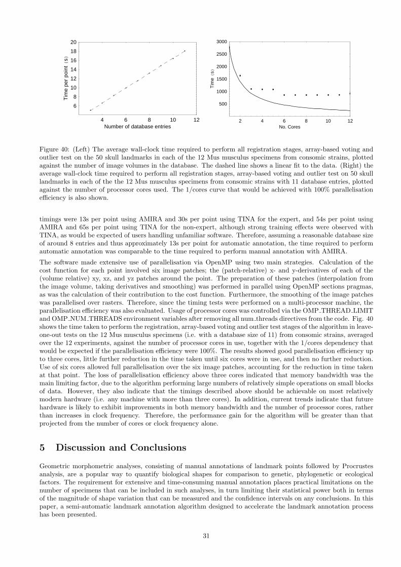
4 6 8 10 12Number of database entries

6

8

10

12

14

16

18

20

Tim

epe

rpo

int(

s)

2 4 6 8 10 12No. Cores

500

1000

1500

2000

2500

3000

Tim

e(

s)

Figure 40: (Left) The average wall-clock time required to perform all registration stages, array-based voting andoutlier test on the 50 skull landmarks in each of the 12 Mus musculus specimens from consomic strains, plottedagainst the number of image volumes in the database. The dashed line shows a linear fit to the data. (Right) theaverage wall-clock time required to perform all registration stages, array-based voting and outlier test on 50 skulllandmarks in each of the the 12 Mus musculus specimens from consomic strains with 11 database entries, plottedagainst the number of processor cores used. The 1/cores curve that would be achieved with 100% parallelisationefficiency is also shown.

timings were 13s per point using AMIRA and 30s per point using TINA for the expert, and 54s per point usingAMIRA and 65s per point using TINA for the non-expert, although strong training effects were observed withTINA, as would be expected of users handling unfamiliar software. Therefore, assuming a reasonable database sizeof around 8 entries and thus approximately 13s per point for automatic annotation, the time required to performautomatic annotation was comparable to the time required to perform manual annotation with AMIRA.

The software made extensive use of parallelisation via OpenMP using two main strategies. Calculation of thecost function for each point involved six image patches; the (patch-relative) x- and y-derivatives of each of the(volume relative) xy, xz, and yz patches around the point. The preparation of these patches (interpolation fromthe image volume, taking derivatives and smoothing) was performed in parallel using OpenMP sections pragmas,as was the calculation of their contribution to the cost function. Furthermore, the smoothing of the image patcheswas parallelised over rasters. Therefore, since the timing tests were performed on a multi-processor machine, theparallelisation efficiency was also evaluated. Usage of processor cores was controlled via the OMP THREAD LIMITand OMP NUM THREADS environment variables after removing all num threads directives from the code. Fig. 40shows the time taken to perform the registration, array-based voting and outlier test stages of the algorithm in leave-one-out tests on the 12 Mus musculus specimens (i.e. with a database size of 11) from consomic strains, averagedover the 12 experiments, against the number of processor cores in use, together with the 1/cores dependency thatwould be expected if the parallelisation efficiency were 100%. The results showed good parallelisation efficiency upto three cores, little further reduction in the time taken until six cores were in use, and then no further reduction.Use of six cores allowed full parallelisation over the six image patches, accounting for the reduction in time takenat that point. The loss of parallelisation efficiency above three cores indicated that memory bandwidth was themain limiting factor, due to the algorithm performing large numbers of relatively simple operations on small blocksof data. However, they also indicate that the timings described above should be achievable on most relativelymodern hardware (i.e. any machine with more than three cores). In addition, current trends indicate that futurehardware is likely to exhibit improvements in both memory bandwidth and the number of processor cores, ratherthan increases in clock frequency. Therefore, the performance gain for the algorithm will be greater than thatprojected from the number of cores or clock frequency alone.

5 Discussion and Conclusions

Geometric morphometric analyses, consisting of manual annotations of landmark points followed by Procrustesanalysis, are a popular way to quantify biological shapes for comparison to genetic, phylogenetic or ecologicalfactors. The requirement for extensive and time-consuming manual annotation places practical limitations on thenumber of specimens that can be included in such analyses, in turn limiting their statistical power both in termsof the magnitude of shape variation that can be measured and the confidence intervals on any conclusions. In thispaper, a semi-automatic landmark annotation algorithm designed to accelerate the landmark annotation processhas been presented.

31

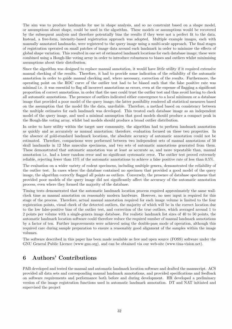
The aim was to produce landmarks for use in shape analysis, and so no constraint based on a shape model,or assumptions about shape, could be used in the algorithm. These models or assumptions would be recoveredby the subsequent analysis and therefore potentially bias the results if they were not a perfect fit to the data.Instead, a free-form, intensity-based registration approach was adopted. Multiple example images, each withmanually annotated landmarks, were registered to the query image using a multi-scale approach. The final stagesof registration operated on small patches of image data around each landmark in order to minimise the effects ofglobal shape variation. This resulted in one set of estimated landmark locations for each database image; these werecombined using a Hough-like voting array in order to introduce robustness to biases and outliers whilst minimisingassumptions about their distribution.

Since the algorithm was designed to replace manual annotation, it would have little utility if it required extensivemanual checking of the results. Therefore, it had to provide some indication of the reliability of the automaticannotation in order to guide manual checking and, where necessary, correction of the results. Furthermore, theoperating point on the ROC curve of the outlier test had to be biased such that the false positive rate wasminimal i.e. it was essential to flag all incorrect annotations as errors, even at the expense of flagging a significantproportion of correct annotations, in order that the user could trust the outlier test and thus avoid having to checkall automatic annotations. The presence of outliers indicated either convergence to a local minimum or a databaseimage that provided a poor model of the query image; the latter possibility rendered all statistical measures basedon the assumption that the model fits the data, unreliable. Therefore, a method based on consistency betweenthe multiple estimates for each landmark was developed. This treated each database image as an independentmodel of the query image, and used a minimal assumption that good models should produce a compact peak inthe Hough-like voting array, whilst bad models should produce a broad outlier distribution.

In order to have utility within the target user community, the algorithm had to perform landmark annotationas quickly and as accurately as manual annotation; therefore, evaluation focused on these two properties. Inthe absence of gold-standard landmark locations, the absolute accuracy of automatic annotation could not beestimated. Therefore, comparisons were performed between two independent sets of manual annotations of 50skull landmarks in 12 Mus musculus specimens, and two sets of automatic annotations generated from them.These demonstrated that automatic annotation was at least as accurate as, and more repeatable than, manualannotation i.e. had a lower random error and no significant systematic error. The outlier test proved extremelyreliable, rejecting fewer than 15% of the automatic annotations to achieve a false positive rate of less than 0.5%.

The evaluation on a wider variety of rodent specimens, including multiple genera, demonstrated the reliability ofthe outlier test. In cases where the database contained no specimen that provided a good model of the queryimage, the algorithm correctly flagged all points as outliers. Conversely, the presence of database specimens thatprovided poor models of the query image did not significantly affect the accuracy of the automatic annotationprocess, even where they formed the majority of the database.

Timing tests demonstrated that the automatic landmark location process required approximately the same wall-clock time as manual annotation on reasonably modern hardware. However, no user input is required for thisstage of the process. Therefore, actual manual annotation required for each image volume is limited to the fourregistration points, visual check of the detected outliers, the majority of which will be in the correct location dueto the low false-positive bias of the outlier test, and correction of the true outliers, which averaged around 1 to2 points per volume with a single-genera image database. For realistic landmark list sizes of 40 to 50 points, theautomatic landmark location software could therefore reduce the required number of manual landmark annotationsby a factor of ten. Further improvements were achieved using the double-pass mode of operation, although thisrequired care during sample preparation to ensure a reasonably good alignment of the samples within the imagevolumes.

The software described in this paper has been made available as free and open source (FOSS) software under theGNU General Public Licence (www.gnu.org), and can be obtained via our web-site (www.tina-vision.net).

6 Authors’ Contributions

PAB developed and tested the manual and automatic landmark location software and drafted the manuscript. ACSprovided all data sets and corresponding manual landmark annotations, and provided specifications and feedbackon software requirements and performance both before and during development. HR developed a preliminaryversion of the image registration functions used in automatic landmark annotation. DT and NAT initiated andsupervised the project

32

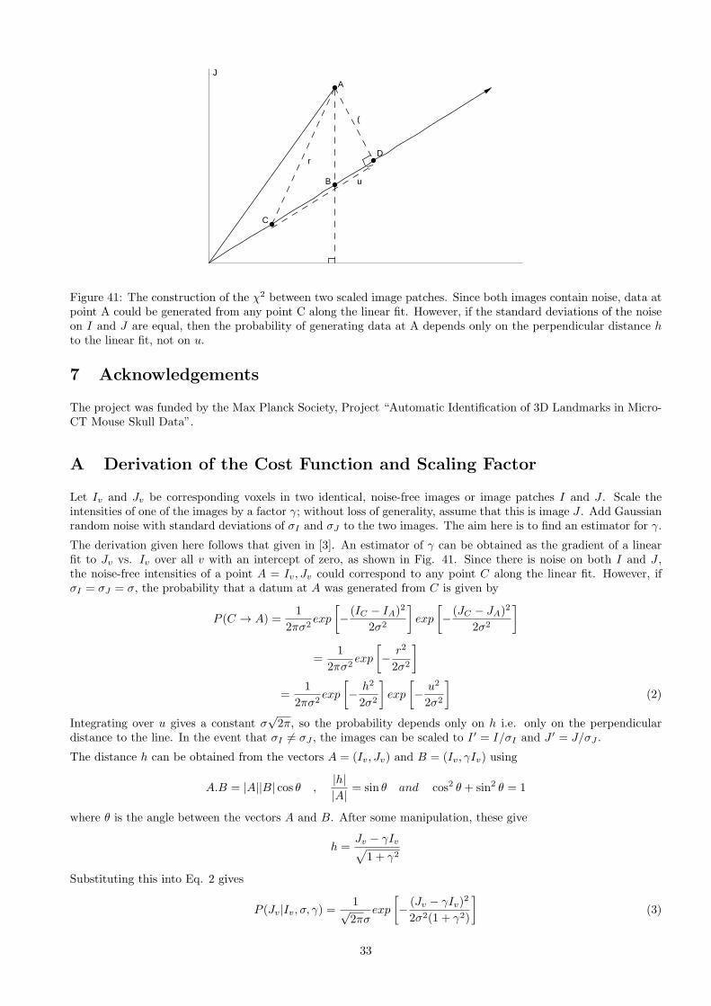
A

B

C

D

I

J

u

r

(

Figure 41: The construction of the χ2 between two scaled image patches. Since both images contain noise, data atpoint A could be generated from any point C along the linear fit. However, if the standard deviations of the noiseon I and J are equal, then the probability of generating data at A depends only on the perpendicular distance hto the linear fit, not on u.

7 Acknowledgements

The project was funded by the Max Planck Society, Project “Automatic Identification of 3D Landmarks in Micro-CT Mouse Skull Data”.

A Derivation of the Cost Function and Scaling Factor

Let Iv and Jv be corresponding voxels in two identical, noise-free images or image patches I and J . Scale theintensities of one of the images by a factor γ; without loss of generality, assume that this is image J . Add Gaussianrandom noise with standard deviations of σI and σJ to the two images. The aim here is to find an estimator for γ.

The derivation given here follows that given in [3]. An estimator of γ can be obtained as the gradient of a linearfit to Jv vs. Iv over all v with an intercept of zero, as shown in Fig. 41. Since there is noise on both I and J ,the noise-free intensities of a point A = Iv, Jv could correspond to any point C along the linear fit. However, ifσI = σJ = σ, the probability that a datum at A was generated from C is given by

P (C → A) =1

2πσ2exp

[

− (IC − IA)2

2σ2

]

exp

[

− (JC − JA)2

2σ2

]

=1

2πσ2exp

[

− r2

2σ2

]

=1

2πσ2exp

[

− h2

2σ2

]

exp

[

− u2

2σ2

]

(2)

Integrating over u gives a constant σ√2π, so the probability depends only on h i.e. only on the perpendicular

distance to the line. In the event that σI 6= σJ , the images can be scaled to I ′ = I/σI and J ′ = J/σJ .

The distance h can be obtained from the vectors A = (Iv, Jv) and B = (Iv, γIv) using

A.B = |A||B| cos θ ,|h||A| = sin θ and cos2 θ + sin2 θ = 1

where θ is the angle between the vectors A and B. After some manipulation, these give

h =Jv − γIv√

1 + γ2

Substituting this into Eq. 2 gives

P (Jv|Iv, σ, γ) =1√2πσ

exp

[

− (Jv − γIv)2

2σ2(1 + γ2)

]

(3)

33

or equivalently

χ2 =∑

v

(Jv − γIv)2

σ2(1 + γ2)∝

∑

v

(Jv − γIv)2

1 + γ2

In order to obtain an estimator for γ, differentiate the χ2 w.r.t. γ and set the result equal to zero. After somemanipulation, this gives

∑

v

γ2IvJv + γ(I2v − J2v )− IvJv

(1 + γ2)2= 0

The numerator in this fraction must be equal to zero, since the denominator cannot be regardless of the value ofγ. Therefore, substituting

|I|2 =∑

v

I2v , |J |2 =∑

v

J2v and I.J =

∑

v

IvJv

givesγ2I.J + γ(|I|2 − |J |2)− I.J = 0

This quadratic can be solved in the usual way to give γ, an estimator for γ

γ =−b±

√b2 − 4ac

2awhere a = I.J , b = |I|2 − |J |2 and c = −I.J

This gives

γ =|J |2 − |I|2 ±

√

(|I|2 − |J |2)2 + 4(I.J)2

2I.J

Now, I.J = |I||J |cosφ where, if the intensities from I and J were concatenated to form two vectors in a v-dimensional space, φ would be the angle between those two vectors. This angle will be small if the signal-to-noiseratio is high, and so assuming that φ ≈ 0,

γ =|J |2 − |I|2 ±

√

(|I|2 + |J |2)22|I||J |

which gives

γ =|J ||I| or γ = − |I|

|J |The two solutions are perpendicular and give the best and worst linear fit to the data. The positive estimator isused when the correlation between I and J is positive, and the negative estimator when the correlation is negative.A negative correlation may be seen with some image modalities, such as MR images acquired with different pulsesequences; however, in the work presented here micro-CT images were used, and so only the positive solution isrelevant. The estimator is both a maximum likelihood and minimum χ2 estimator.

The above derivation also provides the cost function for registration of I and J used in the work described here asEquation 3

χ2 =∑

v

(Jv − γIv)2

σ2(1 + γ2)

This is valid only if the noise on I and J are equal. In the more general case where they are not equal, the imagescan be scaled to to I ′ = I/σI and J ′ = J/σJ ; let γ′ represent γ estimated in the I ′, J ′ space, so that the costfunction becomes

χ2 =∑

v

(Jv/σJ − γ′Iv/σI)2

(1 + γ′2)

Rearranging gives

χ2 =∑

v

(Jv − γ′ σJ

σIIv)

2

σ2J(1 + γ′2)

and, since

γ′ =|J ′||I ′| =

σI

σJ

|J ||I|

letting γ = |J |/|I|, the cost function becomes

χ2 =∑

v

(Jv − γIv)2

σ2J + σ2

Iγ2

34

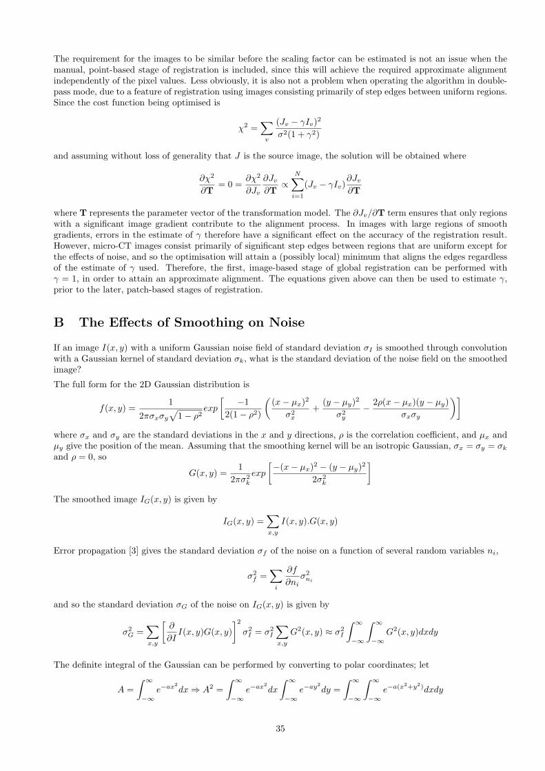
The requirement for the images to be similar before the scaling factor can be estimated is not an issue when themanual, point-based stage of registration is included, since this will achieve the required approximate alignmentindependently of the pixel values. Less obviously, it is also not a problem when operating the algorithm in double-pass mode, due to a feature of registration using images consisting primarily of step edges between uniform regions.Since the cost function being optimised is

χ2 =∑

v

(Jv − γIv)2

σ2(1 + γ2)

and assuming without loss of generality that J is the source image, the solution will be obtained where

∂χ2

∂T= 0 =

∂χ2

∂Jv

∂Jv∂T

∝N∑

i=1

(Jv − γIv)∂Jv∂T

where T represents the parameter vector of the transformation model. The ∂Jv/∂T term ensures that only regionswith a significant image gradient contribute to the alignment process. In images with large regions of smoothgradients, errors in the estimate of γ therefore have a significant effect on the accuracy of the registration result.However, micro-CT images consist primarily of significant step edges between regions that are uniform except forthe effects of noise, and so the optimisation will attain a (possibly local) minimum that aligns the edges regardlessof the estimate of γ used. Therefore, the first, image-based stage of global registration can be performed withγ = 1, in order to attain an approximate alignment. The equations given above can then be used to estimate γ,prior to the later, patch-based stages of registration.

B The Effects of Smoothing on Noise

If an image I(x, y) with a uniform Gaussian noise field of standard deviation σI is smoothed through convolutionwith a Gaussian kernel of standard deviation σk, what is the standard deviation of the noise field on the smoothedimage?

The full form for the 2D Gaussian distribution is

f(x, y) =1

2πσxσy

√

1− ρ2exp

[ −1

2(1− ρ2)

(

(x− µx)2

σ2x

+(y − µy)

2

σ2y

− 2ρ(x− µx)(y − µy)

σxσy

)]

where σx and σy are the standard deviations in the x and y directions, ρ is the correlation coefficient, and µx andµy give the position of the mean. Assuming that the smoothing kernel will be an isotropic Gaussian, σx = σy = σk

and ρ = 0, so

G(x, y) =1

2πσ2k

exp

[−(x− µx)2 − (y − µy)

2

2σ2k

]

The smoothed image IG(x, y) is given by

IG(x, y) =∑

x,y

I(x, y).G(x, y)

Error propagation [3] gives the standard deviation σf of the noise on a function of several random variables ni,

σ2f =

∑

i

∂f

∂ni

σ2ni

and so the standard deviation σG of the noise on IG(x, y) is given by

σ2G =

∑

x,y

[

∂

∂II(x, y)G(x, y)

]2

σ2I = σ2

I

∑

x,y

G2(x, y) ≈ σ2I

∫

∞

−∞

∫

∞

−∞

G2(x, y)dxdy

The definite integral of the Gaussian can be performed by converting to polar coordinates; let

A =

∫

∞

−∞

e−ax2

dx ⇒ A2 =

∫

∞

−∞

e−ax2

dx

∫

∞

−∞

e−ay2

dy =

∫

∞

−∞

∫

∞

−∞

e−a(x2+y2)dxdy

35

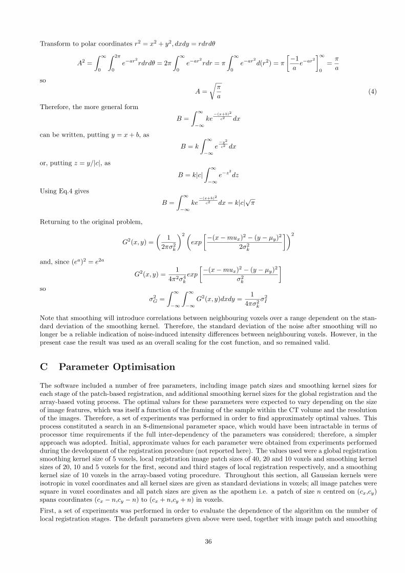
Transform to polar coordinates r2 = x2 + y2, dxdy = rdrdθ

A2 =

∫

∞

0

∫ 2π

0

e−ar2rdrdθ = 2π

∫

∞

0

e−ar2rdr = π

∫

∞

0

e−ar2d(r2) = π

[−1

ae−ar2

]

∞

0

=π

a

so

A =

√

π

a(4)

Therefore, the more general form

B =

∫

∞

−∞

ke−(x+b)2

c2 dx

can be written, putting y = x+ b, as

B = k

∫

∞

−∞

e−y2

c2 dx

or, putting z = y/|c|, asB = k|c|

∫

∞

−∞

e−z2

dz

Using Eq.4 gives

B =

∫

∞

−∞

ke−(x+b)2

c2 dx = k|c|√π

Returning to the original problem,

G2(x, y) =

(

1

2πσ2k

)2 (

exp

[−(x−mux)2 − (y − µy)

2

2σ2k

])2

and, since (ea)2 = e2a

G2(x, y) =1

4π2σ4k

exp

[−(x−mux)2 − (y − µy)

2

σ2k

]

so

σ2G =

∫

∞

−∞

∫

∞

−∞

G2(x, y)dxdy =1

4πσ2k

σ2I

Note that smoothing will introduce correlations between neighbouring voxels over a range dependent on the stan-dard deviation of the smoothing kernel. Therefore, the standard deviation of the noise after smoothing will nolonger be a reliable indication of noise-induced intensity differences between neighbouring voxels. However, in thepresent case the result was used as an overall scaling for the cost function, and so remained valid.

C Parameter Optimisation

The software included a number of free parameters, including image patch sizes and smoothing kernel sizes foreach stage of the patch-based registration, and additional smoothing kernel sizes for the global registration and thearray-based voting process. The optimal values for these parameters were expected to vary depending on the sizeof image features, which was itself a function of the framing of the sample within the CT volume and the resolutionof the images. Therefore, a set of experiments was performed in order to find approximately optimal values. Thisprocess constituted a search in an 8-dimensional parameter space, which would have been intractable in terms ofprocessor time requirements if the full inter-dependency of the parameters was considered; therefore, a simplerapproach was adopted. Initial, approximate values for each parameter were obtained from experiments performedduring the development of the registration procedure (not reported here). The values used were a global registrationsmoothing kernel size of 5 voxels, local registration image patch sizes of 40, 20 and 10 voxels and smoothing kernelsizes of 20, 10 and 5 voxels for the first, second and third stages of local registration respectively, and a smoothingkernel size of 10 voxels in the array-based voting procedure. Throughout this section, all Gaussian kernels wereisotropic in voxel coordinates and all kernel sizes are given as standard deviations in voxels; all image patches weresquare in voxel coordinates and all patch sizes are given as the apothem i.e. a patch of size n centred on (cx,cy)spans coordinates (cx − n,cy − n) to (cx + n,cy + n) in voxels.

First, a set of experiments was performed in order to evaluate the dependence of the algorithm on the number oflocal registration stages. The default parameters given above were used, together with image patch and smoothing

36

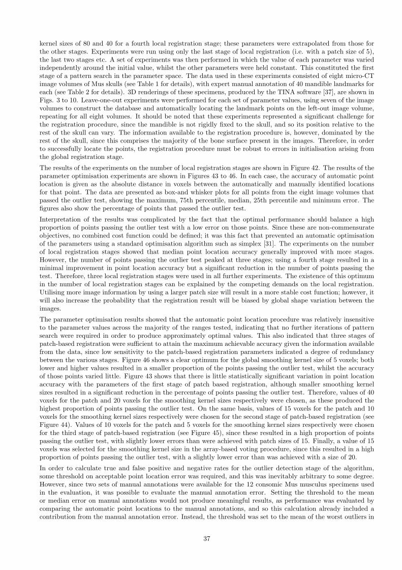
kernel sizes of 80 and 40 for a fourth local registration stage; these parameters were extrapolated from those forthe other stages. Experiments were run using only the last stage of local registration (i.e. with a patch size of 5),the last two stages etc. A set of experiments was then performed in which the value of each parameter was variedindependently around the initial value, whilst the other parameters were held constant. This constituted the firststage of a pattern search in the parameter space. The data used in these experiments consisted of eight micro-CTimage volumes of Mus skulls (see Table 1 for details), with expert manual annotation of 40 mandible landmarks foreach (see Table 2 for details). 3D renderings of these specimens, produced by the TINA software [37], are shown inFigs. 3 to 10. Leave-one-out experiments were performed for each set of parameter values, using seven of the imagevolumes to construct the database and automatically locating the landmark points on the left-out image volume,repeating for all eight volumes. It should be noted that these experiments represented a significant challenge forthe registration procedure, since the mandible is not rigidly fixed to the skull, and so its position relative to therest of the skull can vary. The information available to the registration procedure is, however, dominated by therest of the skull, since this comprises the majority of the bone surface present in the images. Therefore, in orderto successfully locate the points, the registration procedure must be robust to errors in initialisation arising fromthe global registration stage.

The results of the experiments on the number of local registration stages are shown in Figure 42. The results of theparameter optimisation experiments are shown in Figures 43 to 46. In each case, the accuracy of automatic pointlocation is given as the absolute distance in voxels between the automatically and manually identified locationsfor that point. The data are presented as box-and whisker plots for all points from the eight image volumes thatpassed the outlier test, showing the maximum, 75th percentile, median, 25th percentile and minimum error. Thefigures also show the percentage of points that passed the outlier test.

Interpretation of the results was complicated by the fact that the optimal performance should balance a highproportion of points passing the outlier test with a low error on those points. Since these are non-commensurateobjectives, no combined cost function could be defined; it was this fact that prevented an automatic optimisationof the parameters using a standard optimisation algorithm such as simplex [31]. The experiments on the numberof local registration stages showed that median point location accuracy generally improved with more stages.However, the number of points passing the outlier test peaked at three stages; using a fourth stage resulted in aminimal improvement in point location accuracy but a significant reduction in the number of points passing thetest. Therefore, three local registration stages were used in all further experiments. The existence of this optimumin the number of local registration stages can be explained by the competing demands on the local registration.Utilising more image information by using a larger patch size will result in a more stable cost function; however, itwill also increase the probability that the registration result will be biased by global shape variation between theimages.

The parameter optimisation results showed that the automatic point location procedure was relatively insensitiveto the parameter values across the majority of the ranges tested, indicating that no further iterations of patternsearch were required in order to produce approximately optimal values. This also indicated that three stages ofpatch-based registration were sufficient to attain the maximum achievable accuracy given the information availablefrom the data, since low sensitivity to the patch-based registration parameters indicated a degree of redundancybetween the various stages. Figure 46 shows a clear optimum for the global smoothing kernel size of 5 voxels; bothlower and higher values resulted in a smaller proportion of the points passing the outlier test, whilst the accuracyof those points varied little. Figure 43 shows that there is little statistically significant variation in point locationaccuracy with the parameters of the first stage of patch based registration, although smaller smoothing kernelsizes resulted in a significant reduction in the percentage of points passing the outlier test. Therefore, values of 40voxels for the patch and 20 voxels for the smoothing kernel sizes respectively were chosen, as these produced thehighest proportion of points passing the outlier test. On the same basis, values of 15 voxels for the patch and 10voxels for the smoothing kernel sizes respectively were chosen for the second stage of patch-based registration (seeFigure 44). Values of 10 voxels for the patch and 5 voxels for the smoothing kernel sizes respectively were chosenfor the third stage of patch-based registration (see Figure 45), since these resulted in a high proportion of pointspassing the outlier test, with slightly lower errors than were achieved with patch sizes of 15. Finally, a value of 15voxels was selected for the smoothing kernel size in the array-based voting procedure, since this resulted in a highproportion of points passing the outlier test, with a slightly lower error than was achieved with a size of 20.

In order to calculate true and false positive and negative rates for the outlier detection stage of the algorithm,some threshold on acceptable point location error was required, and this was inevitably arbitrary to some degree.However, since two sets of manual annotations were available for the 12 consomic Mus musculus specimens usedin the evaluation, it was possible to evaluate the manual annotation error. Setting the threshold to the meanor median error on manual annotations would not produce meaningful results, as performance was evaluated bycomparing the automatic point locations to the manual annotations, and so this calculation already included acontribution from the manual annotation error. Instead, the threshold was set to the mean of the worst outliers in

37

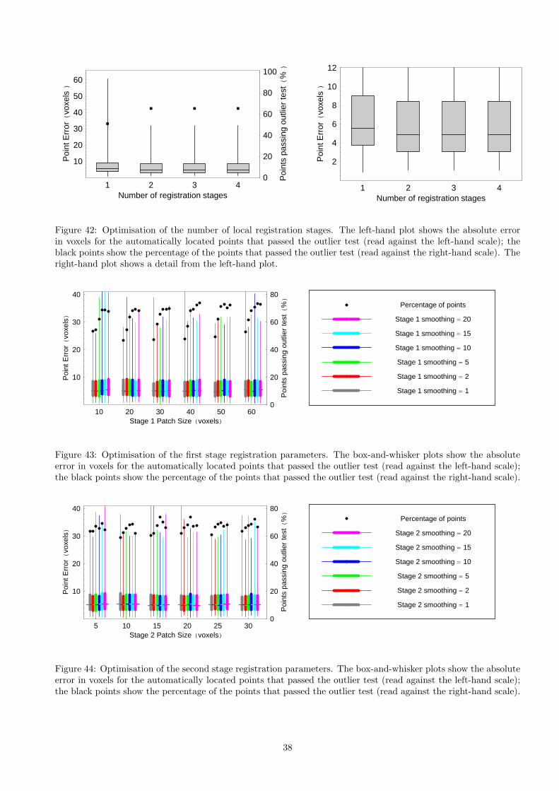
1 2 3 4Number of registration stages

10

20

30

40

50

60

Poi

ntE

rror(

voxe

ls)

0

20

40

60

80

100

Poi

nts

pass

ing

outli

erte

st(

%)

1 2 3 4Number of registration stages

2

4

6

8

10

12

Poi

ntE

rror(

voxe

ls)

Figure 42: Optimisation of the number of local registration stages. The left-hand plot shows the absolute errorin voxels for the automatically located points that passed the outlier test (read against the left-hand scale); theblack points show the percentage of the points that passed the outlier test (read against the right-hand scale). Theright-hand plot shows a detail from the left-hand plot.

10 20 30 40 50 60Stage 1 Patch Size (voxels)

10

20

30

40

Poi

ntE

rror(

voxe

ls)

0

20

40

60

80

Poi

nts

pass

ing

outli

erte

st(

%)

Stage 1 smoothing = 1

Stage 1 smoothing = 2

Stage 1 smoothing = 5

Stage 1 smoothing = 10

Stage 1 smoothing = 15

Stage 1 smoothing = 20

Percentage of points

Figure 43: Optimisation of the first stage registration parameters. The box-and-whisker plots show the absoluteerror in voxels for the automatically located points that passed the outlier test (read against the left-hand scale);the black points show the percentage of the points that passed the outlier test (read against the right-hand scale).

5 10 15 20 25 30Stage 2 Patch Size (voxels)

10

20

30

40

Poi

ntE

rror(

voxe

ls)

0

20

40

60

80

Poi

nts

pass

ing

outli

erte

st(

%)

Stage 2 smoothing = 1

Stage 2 smoothing = 2

Stage 2 smoothing = 5

Stage 2 smoothing = 10

Stage 2 smoothing = 15

Stage 2 smoothing = 20

Percentage of points

Figure 44: Optimisation of the second stage registration parameters. The box-and-whisker plots show the absoluteerror in voxels for the automatically located points that passed the outlier test (read against the left-hand scale);the black points show the percentage of the points that passed the outlier test (read against the right-hand scale).

38

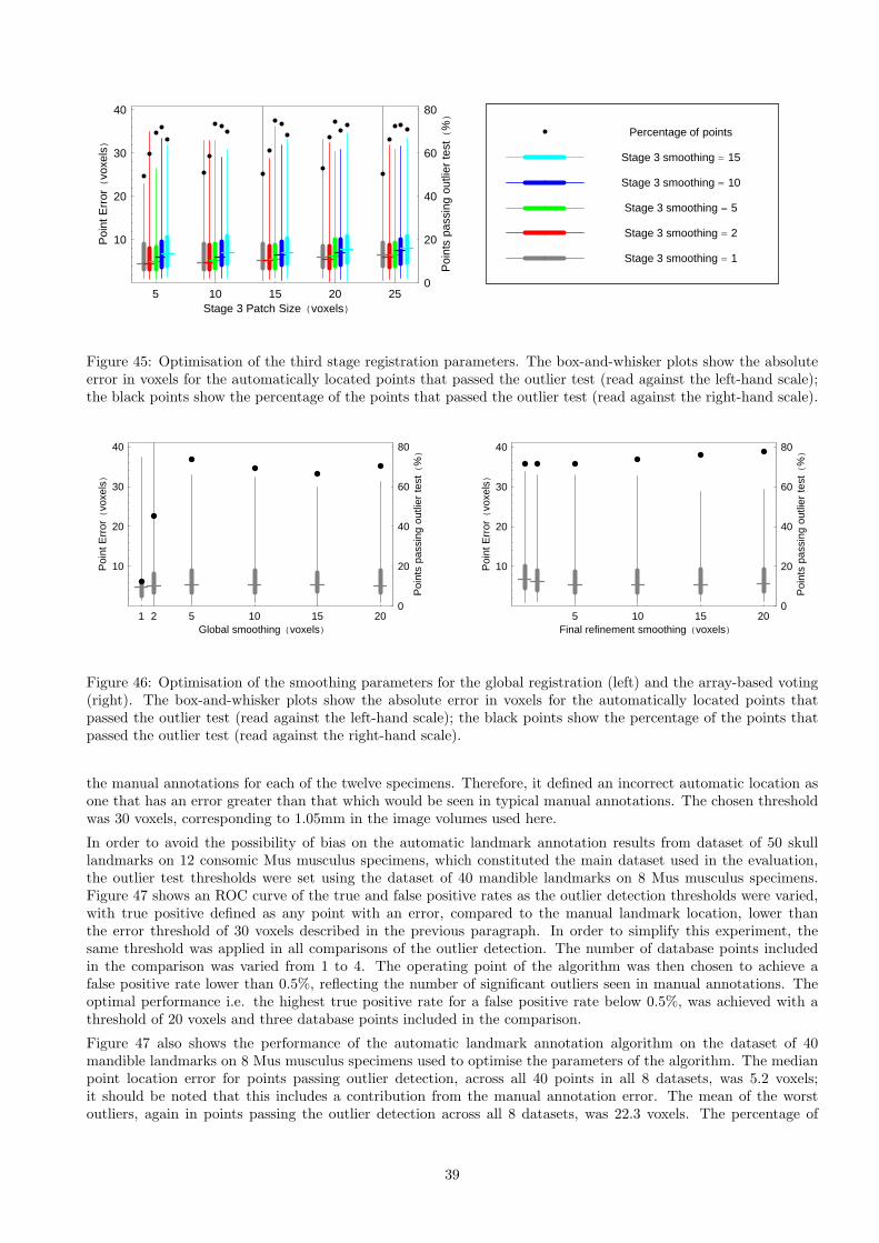
5 10 15 20 25Stage 3 Patch Size (voxels)

10

20

30

40P

oint

Err

or(

voxe

ls)

0

20

40

60

80

Poi

nts

pass

ing

outli

erte

st(

%)

Stage 3 smoothing = 1

Stage 3 smoothing = 2

Stage 3 smoothing = 5

Stage 3 smoothing = 10

Stage 3 smoothing = 15

Percentage of points

Figure 45: Optimisation of the third stage registration parameters. The box-and-whisker plots show the absoluteerror in voxels for the automatically located points that passed the outlier test (read against the left-hand scale);the black points show the percentage of the points that passed the outlier test (read against the right-hand scale).

1 2 5 10 15 20Global smoothing (voxels)

10

20

30

40

Poi

ntE

rror(

voxe

ls)

0

20

40

60

80

Poi

nts

pass

ing

outli

erte

st(

%)

5 10 15 20Final refinement smoothing (voxels)

10

20

30

40

Poi

ntE

rror(

voxe

ls)

0

20

40

60

80

Poi

nts

pass

ing

outli

erte

st(

%)

Figure 46: Optimisation of the smoothing parameters for the global registration (left) and the array-based voting(right). The box-and-whisker plots show the absolute error in voxels for the automatically located points thatpassed the outlier test (read against the left-hand scale); the black points show the percentage of the points thatpassed the outlier test (read against the right-hand scale).

the manual annotations for each of the twelve specimens. Therefore, it defined an incorrect automatic location asone that has an error greater than that which would be seen in typical manual annotations. The chosen thresholdwas 30 voxels, corresponding to 1.05mm in the image volumes used here.

In order to avoid the possibility of bias on the automatic landmark annotation results from dataset of 50 skulllandmarks on 12 consomic Mus musculus specimens, which constituted the main dataset used in the evaluation,the outlier test thresholds were set using the dataset of 40 mandible landmarks on 8 Mus musculus specimens.Figure 47 shows an ROC curve of the true and false positive rates as the outlier detection thresholds were varied,with true positive defined as any point with an error, compared to the manual landmark location, lower thanthe error threshold of 30 voxels described in the previous paragraph. In order to simplify this experiment, thesame threshold was applied in all comparisons of the outlier detection. The number of database points includedin the comparison was varied from 1 to 4. The operating point of the algorithm was then chosen to achieve afalse positive rate lower than 0.5%, reflecting the number of significant outliers seen in manual annotations. Theoptimal performance i.e. the highest true positive rate for a false positive rate below 0.5%, was achieved with athreshold of 20 voxels and three database points included in the comparison.

Figure 47 also shows the performance of the automatic landmark annotation algorithm on the dataset of 40mandible landmarks on 8 Mus musculus specimens used to optimise the parameters of the algorithm. The medianpoint location error for points passing outlier detection, across all 40 points in all 8 datasets, was 5.2 voxels;it should be noted that this includes a contribution from the manual annotation error. The mean of the worstoutliers, again in points passing the outlier detection across all 8 datasets, was 22.3 voxels. The percentage of

39

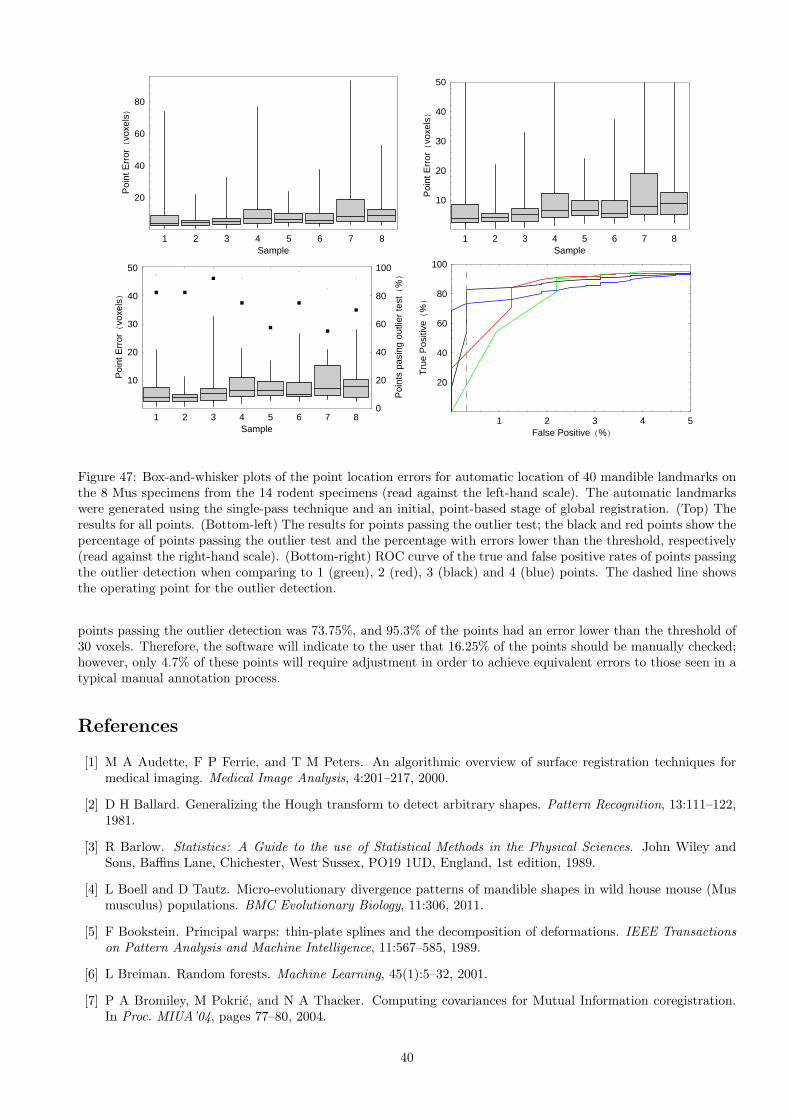
1 2 3 4 5 6 7 8Sample

20

40

60

80

Poi

ntE

rror(

voxe

ls)

1 2 3 4 5 6 7 8Sample

10

20

30

40

50

Poi

ntE

rror(

voxe

ls)

1 2 3 4 5 6 7 8Sample

10

20

30

40

50

Poi

ntE

rror(

voxe

ls)

0

20

40

60

80

100

Poi

nts

pasi

ngou

tlier

test(

%)

1 2 3 4 5False Positive (%)

20

40

60

80

100

Tru

eP

ositi

ve(

%)

Figure 47: Box-and-whisker plots of the point location errors for automatic location of 40 mandible landmarks onthe 8 Mus specimens from the 14 rodent specimens (read against the left-hand scale). The automatic landmarkswere generated using the single-pass technique and an initial, point-based stage of global registration. (Top) Theresults for all points. (Bottom-left) The results for points passing the outlier test; the black and red points show thepercentage of points passing the outlier test and the percentage with errors lower than the threshold, respectively(read against the right-hand scale). (Bottom-right) ROC curve of the true and false positive rates of points passingthe outlier detection when comparing to 1 (green), 2 (red), 3 (black) and 4 (blue) points. The dashed line showsthe operating point for the outlier detection.

points passing the outlier detection was 73.75%, and 95.3% of the points had an error lower than the threshold of30 voxels. Therefore, the software will indicate to the user that 16.25% of the points should be manually checked;however, only 4.7% of these points will require adjustment in order to achieve equivalent errors to those seen in atypical manual annotation process.

References

[1] M A Audette, F P Ferrie, and T M Peters. An algorithmic overview of surface registration techniques formedical imaging. Medical Image Analysis, 4:201–217, 2000.

[2] D H Ballard. Generalizing the Hough transform to detect arbitrary shapes. Pattern Recognition, 13:111–122,1981.

[3] R Barlow. Statistics: A Guide to the use of Statistical Methods in the Physical Sciences. John Wiley andSons, Baffins Lane, Chichester, West Sussex, PO19 1UD, England, 1st edition, 1989.

[4] L Boell and D Tautz. Micro-evolutionary divergence patterns of mandible shapes in wild house mouse (Musmusculus) populations. BMC Evolutionary Biology, 11:306, 2011.

[5] F Bookstein. Principal warps: thin-plate splines and the decomposition of deformations. IEEE Transactionson Pattern Analysis and Machine Intelligence, 11:567–585, 1989.

[6] L Breiman. Random forests. Machine Learning, 45(1):5–32, 2001.

[7] P A Bromiley, M Pokric, and N A Thacker. Computing covariances for Mutual Information coregistration.In Proc. MIUA’04, pages 77–80, 2004.

40

[8] P A Bromiley, M Pokric, and N A Thacker. Emprical evaluation of covariance estimates for Mutual Informationcoregistration. In Proc. MICCAI’04, pages 607–614, 2004.

[9] P A Bromiley, H Ragheb, and N A Thacker. The TINA geometric morphometrics toolkit. http://www.

tina-vision.net/docs/memos/2010-007.pdf.

[10] J Canny. A computational approach to edge detection. IEEE Transactions on Pattern Analysis and MachineIntelligence, 8(6):679–698, 1986.

[11] A Cardini and S Elton. Does the skull carry a phylogenetic signal? Evolution and modularity in the guenons.Biological Journal of the Linnean Society, 93:813–834, 2008.

[12] A Collignon, F Maes, D Delaere, D Vandermeulan, P Suetens, and G Marchal. Automated multi-modalityimage registration based on information theory. In Y Bizais, C Barillot, and R Di Paola, editors, InformationProcessing in Medical Imaging, pages 263–274. Kulwer Academic, Dordrecht, 1995.

[13] J J Condon. Errors in elliptical Gaussian fits. Publications of the Astronomical Society of the Pacific,109(732):166–172, 1997.

[14] T F Cootes, G J Edwards, and C J Taylor. Active appearance models. IEEE Transactions on Pattern Analysisand Machine Intelligence, 23:681–685, 2001.

[15] T F Cootes, M C Ionita, C Lindner, and P Sauer. Robust and accurate shape model fitting using randomforest regression voting. In Proc. ECCV’12, pages 278–291, 2012.

[16] T F Cootes and C J Taylor. Active shape models - ‘smart snakes’. In Proc. British Machine Vision Conference(BMVC’92), pages 266–275, 1992.

[17] T F Cootes, C J Taylor, D Cooper, and J Graham. Active shape models - their training and application.Computer Vision and Image Understanding, 61:38–59, 1995.

[18] D Cristinacce and T F Cootes. Automatic feature localisation with constrained local models. Journal ofComputer Vision, 61:55–79, 2005.

[19] M Erdt, S Steger, and S Wesarg. Deformable registration of MR images using a hierarchical patch based ap-proach with a normalized metric quality measure. In Biomedical Imaging (ISBI), 2012 9th IEEE InternationalSymposium on, pages 1347–1350, 2012.

[20] P Felzenswalb and D Hutenocher. Pictorial structures for object recognition. International Hournal of Com-puter Vision, 61:55–79, 2005.

[21] J Gall and V Lempitsky. Class-specific Hough forests for object detection. In Proc. IEEE Conference onComputer Vision and Pattern Recognition (CVPR’09), pages 1022–1029, 2009.

[22] T Heimann and H Meinzer. Statistical shape models for 3D medical image segmentation: A review. MedicalImage Analysis, 13(4):543–563, 2009.

[23] D L G Hill, P G Batchelor, M Holden, and D J Hawkes. Medical image registration. Physics in Medicine andBiology, 46:R1–R45, 2001.

[24] M Kim, G Wu, and D Shen. Sparse patch-guided deformation estimation for improved image registration. InFei Wang, Dinggang Shen, Pingkun Yan, and Kenji Suzuki, editors, Machine Learning in Medical Imaging,volume 7588 of Lecture Notes in Computer Science, pages 54–62. Springer Berlin Heidelberg, 2012.

[25] P Lacroute and M Levoy. The Volpack volume rendering library. http://graphics.stanford.edu/software/volpack/.

[26] P Lacroute and M Levoy. Fast volume rendering using a shear-warp factorization of the viewing transform.In Proc. SIGGRAPH ’94, July 24-29, Orlando, Florida, pages 451–458, 1994.

[27] Y H Lau, M Braun, and B F Hutton. Non-rigid image registration using a median-filtered coarse-to-finedisplacement field and a symmetric correlation ratio. Physics in Medicine and Biology, 46:12971319, 2001.

[28] U Malsch, C Thieke, P E Huber, and R Bendl. An enhanced block matching algorithm for fast elasticregistration in adaptive radiotherapy. Physics in Medicine and Biology, 51(19):4789–4806, 2006.

41

[29] V R S Mani and S Arivazhagan. Survey of medical image registration. Journal of Biomedical Engineeringand Technology, 1(2):8–25, 2013.

[30] C Meloro and P OHiggins. Ecological adaptations of mandibular form in fissiped carnivora. Journal ofMammalian Evolution, 18:185–200, 2011.

[31] J A Nelder and R Meade. A simplex method for function minimisation. Computer Journal, 7:308–313, 1965.

[32] F P MOliveira and J M R S Tavares. Medical image registration: a review. Computer Methods in Biomechanicsand Biomedical Engineering, pages 1–21, 2012.

[33] S I Olsen. Estimation of noise in images: An evaluation. CVGIP: Graphical Models and Image Processing,55:319–323, 1993.

[34] S Palaniswamy, N A Thacker, and C P Klingenberg. Automatic identification of morphometric landmarks indigital images. In Proc. BMVC’07, 10-13 September, Warwick, U.K., page 112, 2007.

[35] S Palaniswamy, N A Thacker, and C P Klingenberg. Automated landmark extraction in digital images -performance evaluation. In Proc. VIE’08, July 19 - Aug 1, Xi’an, China, 2008.

[36] H Ragheb, N A Thacker, P A Bromiley, D Tautz, and A C Schunke. Quantitative shape analysis with weightedcovariance estimates for increased statistical efficiency. Frontiers in Zoology, 10(16):1–23, 2013.

[37] A C Schunke, P A Bromiley, D Tautz, and N A Thacker. TINA manual landmarking tool: software for theprecise digitization of 3D landmarks. Frontiers in Zoology, 9(6), 2012.

[38] M Sohn, M Birkner, Y Chi, J Wang, D Yan, B Berger, and M Alber. Model-independent, multimodalitydeformable image registration by local matching of anatomical features and minimization of elastic energy.Medical Physics, 35(3):866–878, 2008.

[39] A Sotiras, C Davatzikos, and N Paragios. Deformable medical image registration: A survey. IEEE Transactionson Medical Imaging, 32(7):1153–1190, 2013.

[40] C Studholme, D L G Hill, and D J Hawkes. An overlap invariant entropy measure of 3D medical imagealignment. Pattern Recognition, 32:71–86, 1999.

[41] G K L Tam, Z-Q Cheng, Y-K Lai, F C Langbein, Y Liu, D Marshall, R R Martin, X-F Sun, and P LRosin. Registration of 3D point clouds and meshes: A survey from rigid to nonrigid. IEEE Transactions onVisualization and Computer Graphics, 19(7):1199–1217, 2013.

[42] O van Kaick, H Zhang, G Hamarneh, and D Cohen-Or. A survey on shape correspondence. Computer GraphicsForum, 30(6):1681–1707, 2011.

[43] P Viola and W M Wells. Alignment by maximisation of mutual information. In Proceedings ICCV’95, page 16,1995.

[44] P Viola andWMWells. Alignment by maximisation of mutual information. International Journal of ComputerVision, 24(2):137–154, 1997.

[45] N von Cramon-Taubadel. Global human mandibular variation reflects differences in agricultural and hunter-gatherer subsistance strategies. PNAS, 108(49):19546–19551, 2011.

[46] M V Wyawahare, P M Patil, and H K Abhyankar. Image registration techniques: An overview. InternationalJournal of Signal Processing, Image Processing and Pattern Recognition, 2(3):11–28, 2009.

42