Semi-Annual Report, Feb. 2002

A NEW GENERATION CHEMICAL FLOODING SIMULATOR

Semi-annual Report for the PeriodSept. 1, 2001 – Feb. 28, 2002

By

Gary A. Pope, Kamy Sepehrnoori, and Mojdeh Delshad

Center for Petroleum and Geosystems Engineering

Work Performed under Contract No. DE–FC-26-00BC15314

Sue Mehlhoff, Project Manager

U.S. Dept of Energy

National Petroleum Technology Office

One West Third Street, Suite 1400

Tulsa, OK 74103-3159

Prepared byThe University of Texas

Center for Petroleum and Geosystems EngineeringAustin, TX 78712

ii

A NEW GENERATION CHEMICAL FLOODING SIMULATOR

Contract No. DE–FC-26-00BC15314

The University of TexasAustin, TX, 78712

Contract Date: October 1, 2001Anticipated Completion: August 31, 2004Government Award: $930,801 (Total funding)

Principal Investigators:Gary A. PopeKamy SepehrnooriMojdeh Delshad

Contract Officer:Richard RogusNational Petroleum Technology Office

Reporting Period: Sept. 1, 2001 – Feb. 28, 2002

1

ABSTRACTThe premise of this research is that a general-purpose reservoir simulator for

several improved oil recovery processes can and should be developed so that high-

resolution simulations of a variety of very large and difficult problems can be achieved

using state-of-the-art computing and computers. Such a simulator is not currently

available to the industry. The goal of this proposed research is to develop a new-

generation chemical flooding simulator that is capable of efficiently and accurately

simulating oil reservoirs with at least a million gridblocks in less than one day on

massively parallel computers. Task 1 is the formulation and development of solution

scheme, Task 2 is the implementation of the chemical module, and Task 3 is validation

and application. We have made significant progress on all three tasks and we are on

schedule on both technical and budget. In this report, we will detail our progress on

Tasks 1 through 3 for the first six months of the project.

SUMMARYDuring the past several years, an advanced and efficient reservoir simulation

framework named IPARS, Integrated Parallel Accurate Reservoir Simulator (Parashar et

al., 1997) has been developed by the research team at the University of Texas. IPARS

includes a number of advanced features such as providing all the necessary infrastructure

for physical models, from message passing and input/output to solvers and well handling,

run on a range of platforms, from a single PC with Linux Operating System to massively

parallel machines or clusters of workstation. The framework supports isothermal, three-

dimensional, multiple phases containing multiple species plus an immobile solid rock

phase with adsorbing components. Phase densities and viscosities may be arbitrary

functions of pressure and composition. Porosity and permeability may vary with

location. Physical properties such as relative permeability and capillary pressure are

functions of saturations and rock type. An arbitrary number of wells may be completed

at arbitrary locations. Finite difference formulations with a block-centered grid are

assumed in the framework. The nonlinear difference equations are solved by either fully

implicit or semi-implicit techniques. Both mass balance and volume balance is

supported. Since the portability of the simulator is very important, FORTRAN 77 is used

2

wherever possible. For memory management and user interaction, classical C is used.

Commercial libraries are prohibited except in the graphics front end to the simulator.

The simulator is formulated for a distributed memory, message passing machine. Free-

format keyword input is used for direct data input. The simulator uses a single set of

units to solve the partial differential equations. However, the user may choose any

physically correct units for the input variables and they will then be converted to the

default internal unit using appropriate conversion factor.

The overall structure of IPARS consists of 3 layers:

� Executive layer that consists of routines that direct the overall course of the

simulation

� Work routines that are typically FORTRAN subroutines that perform grid

element computations.

� Data-management layer that handles the distribution of grid across processing

nodes, local storage allocation, dynamic reallocation and dynamic load

balancing, and communication rescheduling. The data-management layer is

also responsible for checkpoint/restart, input/output and visualization.

The fully implicit EOS compositional formulation has already been implemented

into the IPARS framework and successfully tested. The Peng-Robinson EOS is used for

hydrocarbon phase behavior calculations. The linear solvers from PETSc package are

used for the solution of underlying linear equations. The framework provides hooks for

implementing specific physical models. Such hooks bridge the models with the

framework. There are several executive routines, and any communications between the

processors and compositional model are performed in these routines. Many tests have

been performed using the EOS compositional simulator on variety of computer platforms

such as IBM SP and a cluster of PCs (Wang et al., 1999).

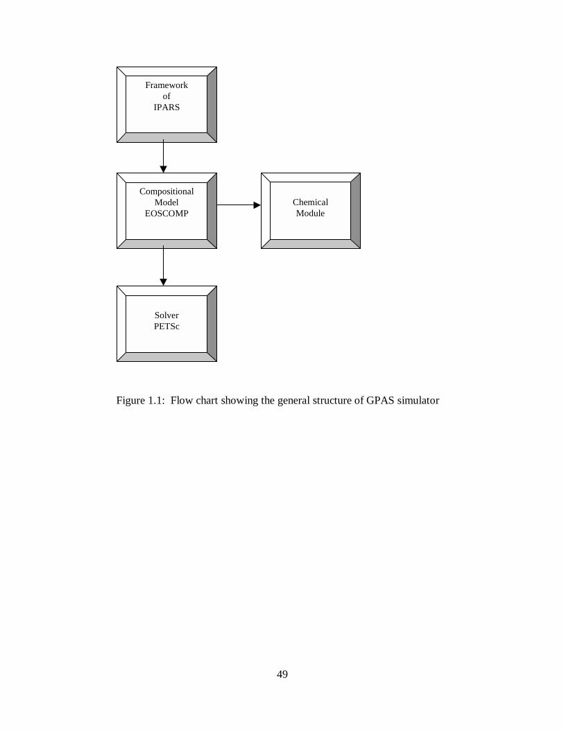
The goal of this project is to add a chemical module to the existing compositional

Peng-Robinson cubic equation of state (EOS). The simulator called GPAS, General

Purpose Adaptive Reservoir Simulator, will then include the IPARS framework, and the

3

compositional and chemical modules as illustrated in Figure 1.1. In this report, we will

detail our progress on Tasks 1 through 3 for the first six months of the project.

Task 1: Formulation and Development of Solution Scheme

The effort on this task was directed towards the formulation of tracer and polymer

options. For completeness, we first give a brief review of the mathematical formulation

of the compositional model. The assumptions made in developing the formulation are:

� Reservoir is isothermal.

� Darcy's law describes the multiphase flow of fluids through the porous media.

� Impermeable zones represented by the no-flow boundaries surround the reservoir.

� The injection and production of fluids are treated as source or sink terms.

� The rock is slightly compressible and immobile.

� Each hydrocarbon phase is composed of nc hydrocarbon components, which may

include the non-hydrocarbon components such as CO2, N2 or H2S.

� Instantaneous local thermodynamic equilibrium between hydrocarbon phases.

� Negligible capillary pressure effects on hydrocarbon phase equilibrium.

� Water is slightly compressible and water viscosity is constant.

Mass conservation equation

The general mass conservation equation for species i in a volume V can be

expressed as

{Rate of accumulation of i in V }

= {Rate of i transported into V }

- {Rate of i transported from V }

+ {Rate of production of i in V }, i = 1,…., cN

(1)

The differential form for the species conservation equation can be expressed as:

4

0��

�

iii RN

tW

(2)

where iW is the overall concentration of i in units of mass of i per unit bulk

volume, iN is the flux vector of species i in units of mass of i per surface area-time and

iR is the mass rate of production in units of mass of i per bulk volume-time.

The mass balance equation can be expressed in terms of moles per unit time by

defining each term of Equation (2 in terms of the porous media and fluid properties such

as porosity, permeability, density, saturations, compositions, rates etc. The accumulation

term for a porous medium becomes

��

�

pn

jijjji xSW

1�� (3)

where � is the porosity, j� is the molar density of phase j , jS is the saturation of phase

j and ijx is the mole fraction of component i in phase j .

The flux vector of component i is a sum of the convective and the dispersive

flux, and can be expressed as

��

��

pn

jijijjjjijj xKSuxN

1�� (4)

where ju represents the superficial velocity or flux of phase j . The flux is evaluated

using the Darcy's law for multiphase flow of fluids through porous media.

)( DPKu jjrjj �� (5)

Darcy's law is a fundamental relationship describing the flow of fluids in

permeable media under laminar flow conditions. The differential form of Darcy's law

can be used to treat multiphase unsteady state flow, non-uniform permeability, non-

uniform pressure gradients. It is used to govern the transport of phases from one cell to

another under the local pressure gradient, rock permeability, relative permeability and

viscosity. Converting each of the terms in the mass balance equation to units of moles

per unit time and expressing the flux using Darcy's law, the mass balance for each

component i is the following partial differential equation:

5

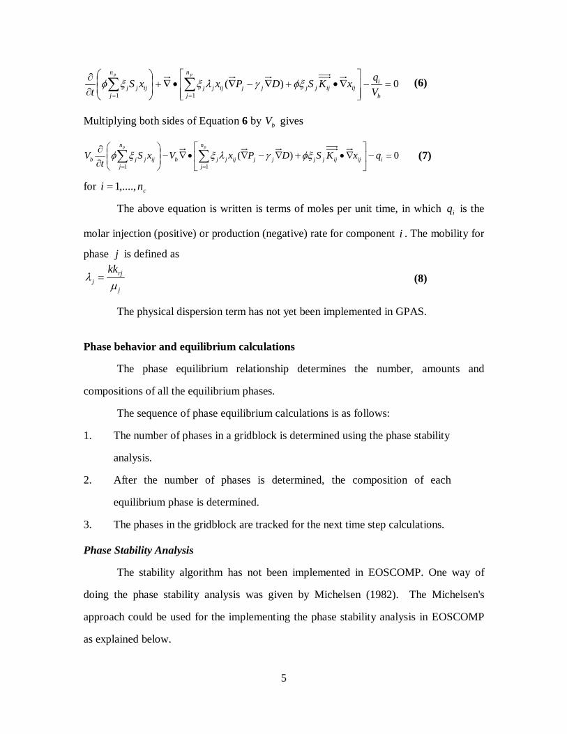
0)(11

��

�

��

��

�

�

��

�

�

�

�� b

in

jijijjjjjijjj

n

jijjj V

qxKSDPxxSt

pp

�� (6)

Multiplying both sides of Equation 6 by bV gives

0)(11

��

��

��

�

��

�

�

��

i

n

jijijjjjjijjjb

n

jijjjb qxKSDPxVxS

tV

pp

��

for cni ,....,1�

(7)

The above equation is written is terms of moles per unit time, in which iq is the

molar injection (positive) or production (negative) rate for component i . The mobility for

phase j is defined as

j

rjj

kk�

� � (8)

The physical dispersion term has not yet been implemented in GPAS.

Phase behavior and equilibrium calculations

The phase equilibrium relationship determines the number, amounts and

compositions of all the equilibrium phases.

The sequence of phase equilibrium calculations is as follows:

1. The number of phases in a gridblock is determined using the phase stability

analysis.

2. After the number of phases is determined, the composition of each

equilibrium phase is determined.

3. The phases in the gridblock are tracked for the next time step calculations.

Phase Stability Analysis

The stability algorithm has not been implemented in EOSCOMP. One way of

doing the phase stability analysis was given by Michelsen (1982). The Michelsen's

approach could be used for the implementing the phase stability analysis in EOSCOMP

as explained below.

6

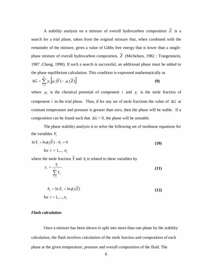
A stability analysis on a mixture of overall hydrocarbon composition Z is a

search for a trial phase, taken from the original mixture that, when combined with the

remainder of the mixture, gives a value of Gibbs free energy that is lower than a single-

phase mixture of overall hydrocarbon composition, Z (Michelsen, 1982 ; Trangenstein,

1987 ,Chang, 1990). If such a search is successful, an additional phase must be added to

the phase equilibrium calculation. This condition is expressed mathematically as

� ��

��

cn

iiii ZYyG

1)()( �� (9)

where i� is the chemical potential of component i and iy is the mole fraction of

component i in the trial phase. Thus, if for any set of mole fractions the value of G� at

constant temperature and pressure is greater than zero, then the phase will be stable. If a

composition can be found such that G� < 0, the phase will be unstable.

The phase stability analysis is to solve the following set of nonlinear equations for

the variables iY

0)(lnln �� iii hYY �

for i = 1,.., cn

(10)

where the mole fraction Y and ih is related to these variables by

��

�

cn

is

ii

Y

Yy

1

(11)

)(lnln ZZh iii ��

for cni ,....,1�

(12)

Flash calculation

Once a mixture has been shown to split into more than one phase by the stability

calculation, the flash involves calculation of the mole fraction and composition of each

phase at the given temperature, pressure and overall composition of the fluid. The

7

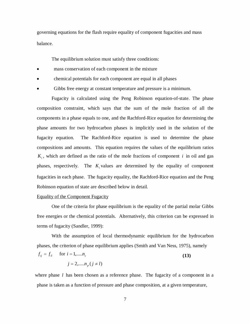
governing equations for the flash require equality of component fugacities and mass

balance.

The equilibrium solution must satisfy three conditions:

� mass conservation of each component in the mixture

� chemical potentials for each component are equal in all phases

� Gibbs free energy at constant temperature and pressure is a minimum.

Fugacity is calculated using the Peng Robinson equation-of-state. The phase

composition constraint, which says that the sum of the mole fraction of all the

components in a phase equals to one, and the Rachford-Rice equation for determining the

phase amounts for two hydrocarbon phases is implicitly used in the solution of the

fugacity equation. The Rachford-Rice equation is used to determine the phase

compositions and amounts. This equation requires the values of the equilibrium ratios

iK , which are defined as the ratio of the mole fractions of component i in oil and gas

phases, respectively. The iK values are determined by the equality of component

fugacities in each phase. The fugacity equality, the Rachford-Rice equation and the Peng

Robinson equation of state are described below in detail.

Equality of the Component Fugacity

One of the criteria for phase equilibrium is the equality of the partial molar Gibbs

free energies or the chemical potentials. Alternatively, this criterion can be expressed in

terms of fugacity (Sandler, 1999):

With the assumption of local thermodynamic equilibrium for the hydrocarbon

phases, the criterion of phase equilibrium applies (Smith and Van Ness, 1975), namely

ilij ff � for cni ,.....1�

)(,.....2 ljnj p ��

(13)

where phase l has been chosen as a reference phase. The fugacity of a component in a

phase is taken as a function of pressure and phase composition, at a given temperature,

8

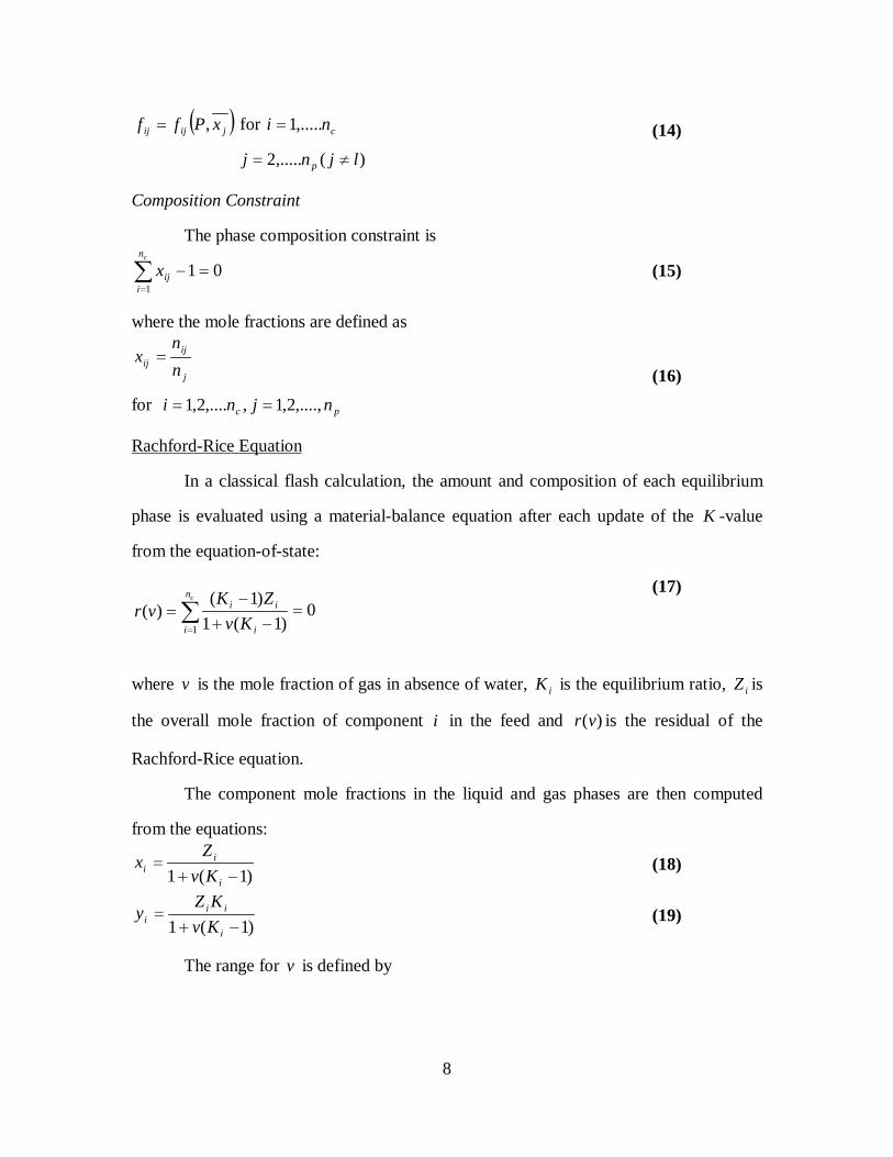
� �jijij xPff ,� for cni ,.....1�

)(,.....2 ljnj p ��

(14)

Composition Constraint

The phase composition constraint is

011

��

cn

iijx

where the mole fractions are defined as

j

ijij n

nx �

for pc njni ,....,2,1,,....2,1 ��

(15)

(16)

Rachford-Rice Equation

In a classical flash calculation, the amount and composition of each equilibrium

phase is evaluated using a material-balance equation after each update of the K -value

from the equation-of-state:

��

�

��

�

�

cn

i i

ii

KvZK

vr1

0)1(1

)1()(

(17)

where v is the mole fraction of gas in absence of water, iK is the equilibrium ratio, iZ is

the overall mole fraction of component i in the feed and )(vr is the residual of the

Rachford-Rice equation.

The component mole fractions in the liquid and gas phases are then computed

from the equations:

)1(1 ��

�

i

ii Kv

Zx (18)

)1(1 ��

�

i

iii Kv

KZy (19)

The range for v is defined by

9

01

1

01

1

min

max

�

�

�

�

�

�

Kv

Kv

r

l (20)

Equation 17 is a monotonically decreasing function of v with asymptotes at

lv and rv . Usually, a Newton iteration can efficiently solve Equations 18 and 19 for v .

However, round-off errors occur when solving Equation 17.

Leibovici and Neoschil Equation

EOSCOMP solves the Rachford-Rice Equation. As was described above, round-

off errors occur when solving the Rachford-Rice equation. To avoid the round off errors

that occur when solving Equation 17, the original Rachford-Rice equation can be

changed into a form that is more nearly linear with respect to v as done by Leibovici and

Neoschil (1992) and this approach could be implemented in EOSCOMP. The Leibovici

and Neoschil equation is given by:

��

�

��

�

��

cn

i i

iirl K

ZKr

10

)1(1)1(

))(()(~�

�� (21)

The range for v is defined by

��

��

�

�

��

11

maxmini

ii

KKZ

v

for 1�iK and 0�iZ

(22)

��

��

�

�

��

11

minmaxi

i

KZ

v

for 1�iK and 0�iZ

(23)

Also, the Newton procedure is used to solve Equation 21 for v .

Equation of State

The Peng Robinson equation of state ( Peng and Robinson, 1976 ) is

)()()(

bVbbVVTa

bVRTP

��

�

�

� (24)

The parameters a and b for a pure component are computed from

10

)(45724.0)(22

TPTR

Tac

c�� (25)

��

�

�

��

�

��

cTT11 �� (26)

c

c

PRTb 07780.0� (27)

226992.054226.137464.0 �� ,

if 49.0��

(28)

32 0.016666 + 0.164423 - 1.485030 + 0.379640 ��

if 49.0��

(29)

For a multi component mixture, the mixing rules for the two parameters are

�

��

�

� �

�

��

c

c c

N

iii

N

i

N

jijjiji

bxb

and

kaaxxa

1

1 1)1(

(30)

where for component i , the ia is computed from Equation 25, and ib is computed from

Equation 27 The constant, ijk is called the binary interaction coefficient between

components i and j .

The Peng Robinson Equation of state can be written in the form

023�� ZZZ (31)

where RT

VPZ � is the compressibility factor, and the parameters are expressed as

B�� 1� (32)

BBA 23 2�� (33)

32 BBAB �� (34)

2)(RTaPA � (35)

RTbPB � (36)

11

In GPAS, the equation-of-state calculations are done in the subroutine named

XEOS, which contains the four subroutines EOSPURE, EOSMIX, EOSPHI and

EOSPARTIAL. The equation-of-state parameters for each pure component are

calculated in the subroutine EOSPURE. Mixture values are calculated in the subroutine

EOSMIX. The fugacity coefficient is calculated from the equation-of-state in the

subroutine EOSPHI and the equation-of-state related derivatives are computed in the

EOSPARTIAL subroutine. The subroutine EOSCUB solves the Peng Robinson cubic

equation-of-state and calculates the compressibility factor and its derivative. EOSCOMP

requires the pure component critical temperature, critical pressure, critical volume,

acentric factors, molecular weights and binary interaction coefficients to calculate the

equation of state parameters. The volume shift parameter is not implemented in GPAS.

The main flash subroutine in GPAS is XFLASH. This subroutine performs the

flash calculation at a given initial composition, temperature and pressure. The number of

components, binary interaction coefficients and the equilibrium ratio values are also part

of the input to this subroutine. An initial estimate of the equilibrium values is done in the

subroutine STABL, which is then passed to the flash calculations. The flash subroutine

calculates the liquid and vapor phase mole fractions, liquid and vapor compressibility

factors, and also the negative residual of component i in cell k . The subroutine SOLVE

solves the Rachford-Rice equation for finding the phase composition and the phase

amounts.

Phase identification and tracking

Phase identification deals with the labeling of a phase as oil, gas, or aqueous

phase at the initial conditions and also when a new phase appears. After a phase has been

identified, phase tracking does the labeling of a phase during the simulation. Labeling

phases consistently is important because of the need to assign a consistent relative

permeability to each phase during a numerical simulation. Perschke (1988) developed a

12

method for the phase identification and tracking in which both phase mass density and

phase composition are used. This is the procedure followed in GPAS. Once a phase has

been identified, it is tracked during simulation by comparing the mole fraction value of a

selected or key component in the equilibrium phases at the new time step with the values

at the old time step. The phases at the new time step are labeled such that the mole

fraction values are closest to the values at the old time step.

The algorithm used in GPAS for naming a phase when the hydrocarbon mixture is

a single phase is similar to that proposed by Gosset et al. (1996). The parameters A and

B of a two-parameter cubic EOS are computed from

�2

2

2)( TPPT

RTaPA

c

ca�� (37)

TPPT

RTbPB

c

cb�� (38)

where

077796074.0457235529.0

��

��

b

a

Dividing Equation 37 by Equation 38 gives:

�

TT

BA

b

ca

�

�� (39)

where � is defined in Equation 26.

A fluid is assumed to be in single-phase if cTT � , which also implies 1�� .

From Equation 39, this implies

b

a

BA

�

�� (40)

or its molar volume to be greater than the critical molar volume, cvv � , which implies

b

cBZZ�

� (41)

In GPAS, the subroutine EOS_1PH identifies a single phase as oil or gas using

the above method. Also, an option is provided in the code to identify a single phase by

13

the conventional method: The fluid is liquid when sum of 1�ii KZ , and the fluid is gas

when the sum of 1/ �ii KZ .

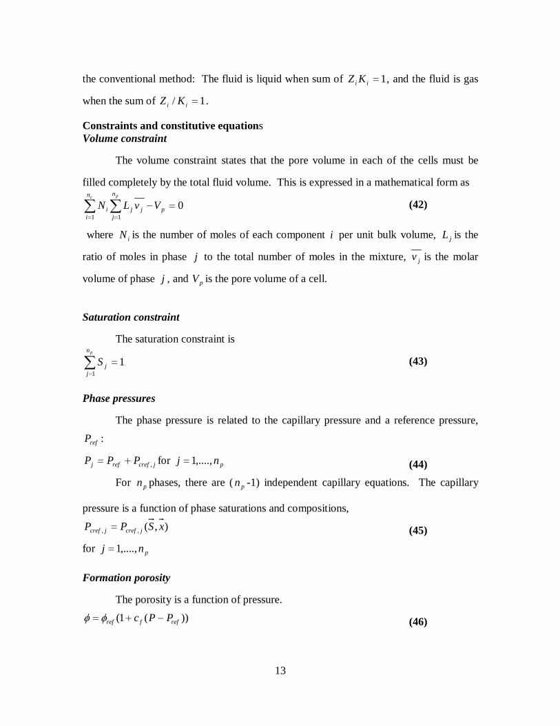
Constraints and constitutive equationsVolume constraint

The volume constraint states that the pore volume in each of the cells must be

filled completely by the total fluid volume. This is expressed in a mathematical form as

01 1

��

p

n

i

n

jjji VvLN

c p

(42)

where iN is the number of moles of each component i per unit bulk volume, jL is the

ratio of moles in phase j to the total number of moles in the mixture, jv is the molar

volume of phase j , and pV is the pore volume of a cell.

Saturation constraint

The saturation constraint is

11

��

pn

jjS (43)

Phase pressures

The phase pressure is related to the capillary pressure and a reference pressure,

refP :

jcrefrefj PPP ,�� for pnj ,....,1� (44)For pn phases, there are ( pn -1) independent capillary equations. The capillary

pressure is a function of phase saturations and compositions,

),(,, xSPP jcrefjcref �

for pnj ,....,1�

(45)

Formation porosity

The porosity is a function of pressure.

))(1( reffref PPc �� (46)

14

where ref� is the porosity at the reference pressure, Pref and � is calculated at the pressure

P.

In GPAS, the porosity calculation is performed in the subroutine AQUEOUS.

The AQUEOUS subroutine also calculates the aqueous phase molar and mass densities.

Physical property models

In this section, the physical models implemented in GPAS to calculate the

viscosities, interfacial tension, relative permeability, capillary pressure, phase molar

density and the hydrocarbon solubility in water are described.

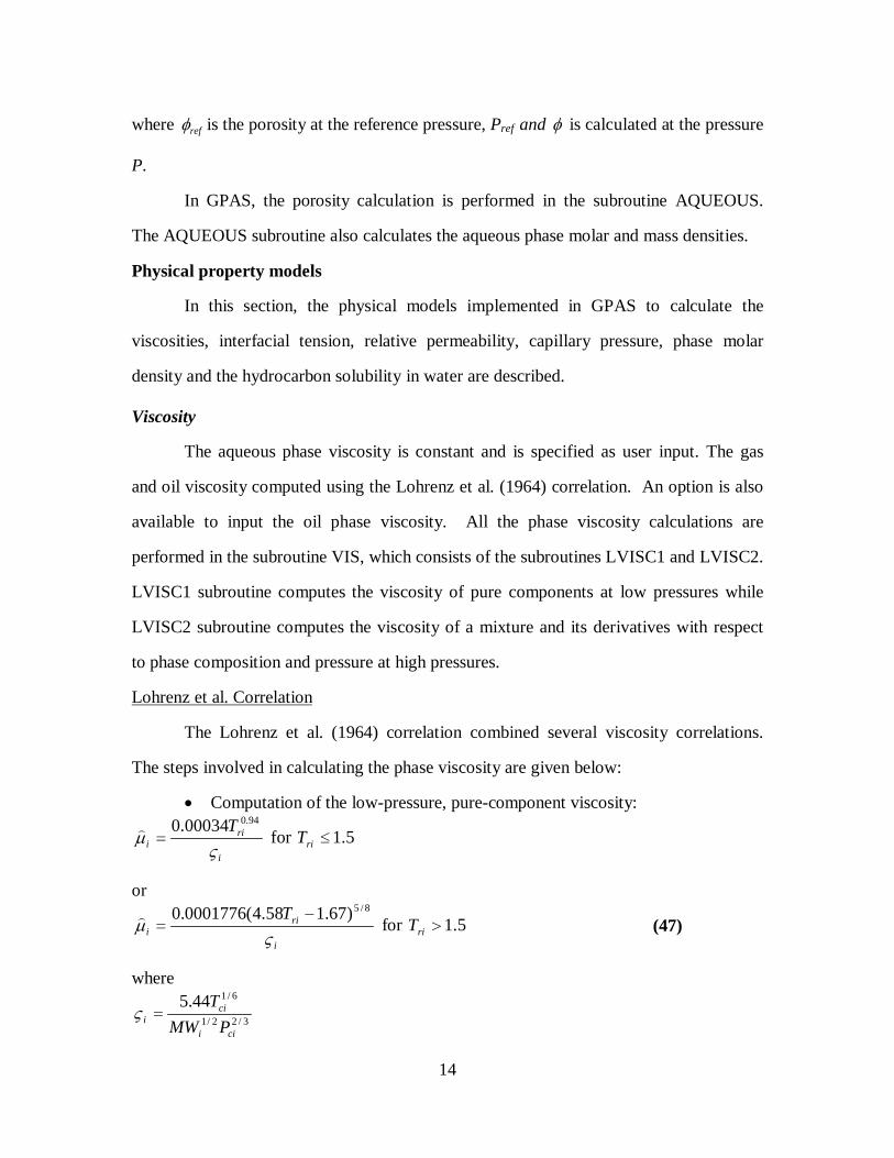
Viscosity

The aqueous phase viscosity is constant and is specified as user input. The gas

and oil viscosity computed using the Lohrenz et al. (1964) correlation. An option is also

available to input the oil phase viscosity. All the phase viscosity calculations are

performed in the subroutine VIS, which consists of the subroutines LVISC1 and LVISC2.

LVISC1 subroutine computes the viscosity of pure components at low pressures while

LVISC2 subroutine computes the viscosity of a mixture and its derivatives with respect

to phase composition and pressure at high pressures.

Lohrenz et al. Correlation

The Lohrenz et al. (1964) correlation combined several viscosity correlations.

The steps involved in calculating the phase viscosity are given below:

� Computation of the low-pressure, pure-component viscosity:

i

rii

T�

�

94.000034.0�

� for 5.1�riT

or

i

rii

T�

�

8/5)67.158.4(0001776.0 ��

� for 5.1�riT

where

(47)

3/22/1

6/144.5

cii

cii PMW

T��

15

� Calculation of the low pressure viscosity :

�

�

�

�

�

c

c

n

iiij

n

iiiij

j

MWx

MWx

1

1*�

�

�

(48)

� The reduced phase molar density calculation

3/2

1

2/1

1

6/1

1

1

44.5

��

��

��

��

�

��

��

�

�

�

��

�

�

��

�

�

cc

c

c

n

iciij

n

iiij

n

iciij

j

n

iciijjjr

PxMWx

Tx

Vx

�

�� (49)

� The Phase viscosity calculation at the desired pressure

j

jrjj

�

�� 000205.0*

�� for 18.0�jr�

j

jjj

�

�� 4

4*

10)1( ��

� for 18.0�jr� (50)

432 093324.040758.058533.023364.0023.1 jrjrjrjrj

where��

Interfacial Tension

The interfacial tension between two hydrocarbon phases is calculated from the

Macleod-Sudgen correlation as reported in Reid, Prausnitz and Poling (1987):4

1)(016018.0 ��

��

��

�

cn

iillijjijl xx �� (51)

where i� is the parachor of component i.

In GPAS, the interfacial tension between gas and oil for gridblock k and the

derivatives of the interfacial tension are calculated in the subroutine IFT.

16

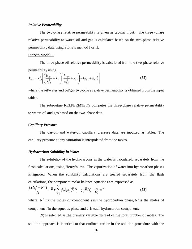
Relative Permeability

The two-phase relative permeability is given as tabular input. The three -phase

relative permeability to water, oil and gas is calculated based on the two-phase relative

permeability data using Stone’s method I or II.

Stone’s Model II

The three-phase oil relative permeability is calculated from the two-phase relative

permeability using

� ��

�

��

��

��

��

��

�� 3130

2

2310

2

21022 rrr

r

rr

r

rrr kkk

kkk

kkkk (52)

where the oil/water and oil/gas two-phase relative permeability is obtained from the input

tables.

The subroutine RELPERM3EOS computes the three-phase relative permeability

to water, oil and gas based on the two-phase data.

Capillary Pressure

The gas-oil and water-oil capillary pressure data are inputted as tables. The

capillary pressure at any saturation is interpolated from the tables.

Hydrocarbon Solubility in Water

The solubility of the hydrocarbons in the water is calculated, separately from the

flash calculations, using Henry’s law. The vaporization of water into hydrocarbon phases

is ignored. When the solubility calculations are treated separately from the flash

calculations, the component molar balance equations are expressed as

��

��

��pn

j b

ijjijjj

ai

hi

VqDPx

tNN

10)()(

�� (53)

where hiN is the moles of component i in the hydrocarbon phase, a

iN is the moles of

component i in the aqueous phase and i is each hydrocarbon component.hiN is selected as the primary variable instead of the total number of moles. The

solution approach is identical to that outlined earlier in the solution procedure with the

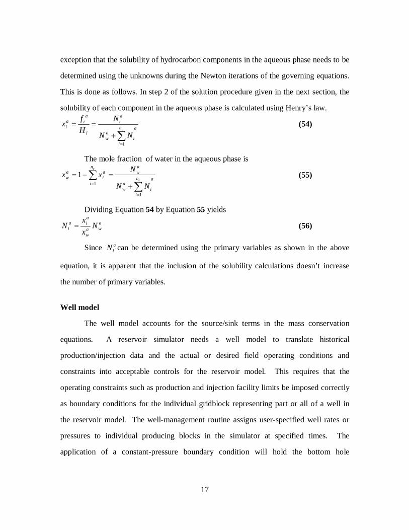
17

exception that the solubility of hydrocarbon components in the aqueous phase needs to be

determined using the unknowns during the Newton iterations of the governing equations.

This is done as follows. In step 2 of the solution procedure given in the next section, the

solubility of each component in the aqueous phase is calculated using Henry’s law.

��

�

��cn

i

a

iaw

ai

i

aia

i

NN

NHf

x

1

(54)

The mole fraction of water in the aqueous phase is

��

�

�

�

��c

c

n

i

a

iaw

aw

n

i

ai

aw

NN

Nxx

1

1

1 (55)

Dividing Equation 54 by Equation 55 yieldsawa

w

aia

i Nxx

N � (56)

Since aiN can be determined using the primary variables as shown in the above

equation, it is apparent that the inclusion of the solubility calculations doesn’t increase

the number of primary variables.

Well model

The well model accounts for the source/sink terms in the mass conservation

equations. A reservoir simulator needs a well model to translate historical

production/injection data and the actual or desired field operating conditions and

constraints into acceptable controls for the reservoir model. This requires that the

operating constraints such as production and injection facility limits be imposed correctly

as boundary conditions for the individual gridblock representing part or all of a well in

the reservoir model. The well-management routine assigns user-specified well rates or

pressures to individual producing blocks in the simulator at specified times. The

application of a constant-pressure boundary condition will hold the bottom hole

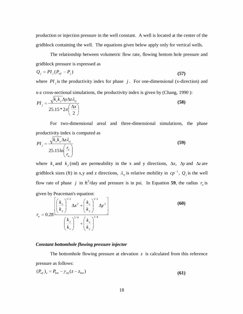
18

production or injection pressure in the well constant. A well is located at the center of the

gridblock containing the well. The equations given below apply only for vertical wells.

The relationship between volumetric flow rate, flowing bottom hole pressure and

gridblock pressure is expressed as

)( jwfjj PPPIQ �� (57)where jPI is the productivity index for phase j . For one-dimensional (x-direction) and

x-z cross-sectional simulations, the productivity index is given by (Chang, 1990 ):

��

��

� �

��

22*15.25 x

zykkPI rjyx

j

�

� (58)

For two-dimensional areal and three-dimensional simulations, the phase

productivity index is computed as

��

��

�

��

w

o

rjyxj

rr

zkkPI

ln15.25

� (59)

where xk and yk (md) are permeability in the x and y directions, ,x� y� and z� are

gridblock sizes (ft) in x,y and z directions, rj� is relative mobility in 1�cp , jQ is the well

flow rate of phase j in ft3/day and pressure is in psi. In Equation 59, the radius or is

given by Peaceman's equation:

4/14/1

2

2/1

2

2/1

28.0

��

�

�

��

�

��

�

��

�

��

��

�

�

��

�

�

��

�

��

��

�

�

��

�

�

�

y

x

x

y

y

x

y

x

o

kk

kk

ykkx

kk

r

(60)

Constant bottomhole flowing pressure injector

The bottomhole flowing pressure at elevation z is calculated from this reference

pressure as follows:

)()( botinjbotzwf zzPP �� (61)

19

where inj� is the specific weight of the injected fluid at the well pressure. The

bottomhole reference depth for each well can be assigned in the input file.

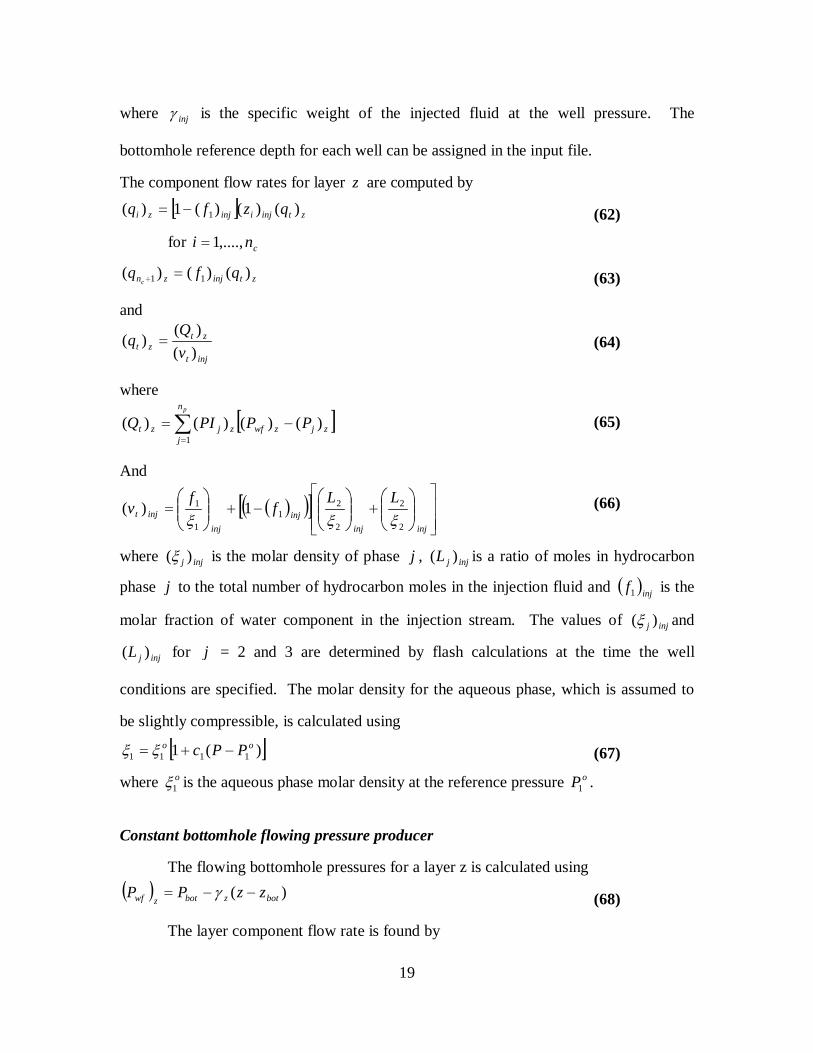
The component flow rates for layer z are computed by

� � ztinjiinjzi qzfq )()()(1)( 1��

for cni ,....,1�

(62)

ztinjzn qfqc

)()()( 11 �� (63)

and

injt

ztzt v

Qq)()(

)( � (64)

where

� ��

��

pn

jzjzwfzjzt PPPIQ

1)()()()( (65)

And

� ��

�

�

��

�

�

��

�

� ��

�

�

��

�

�

��

injinjinj

injinjt

LLf

fv

2

2

2

21

1

1 1)(��

(66)

where injj )(� is the molar density of phase j , injjL )( is a ratio of moles in hydrocarbon

phase j to the total number of hydrocarbon moles in the injection fluid and � �injf1 is the

molar fraction of water component in the injection stream. The values of injj )(� and

injjL )( for j = 2 and 3 are determined by flash calculations at the time the well

conditions are specified. The molar density for the aqueous phase, which is assumed to

be slightly compressible, is calculated using

� �)(1 1111oo PPc �� (67)

where o1� is the aqueous phase molar density at the reference pressure oP1 .

Constant bottomhole flowing pressure producer

The flowing bottomhole pressures for a layer z is calculated using� � )( botzbotzwf zzPP �� (68)

The layer component flow rate is found by

20

��

��

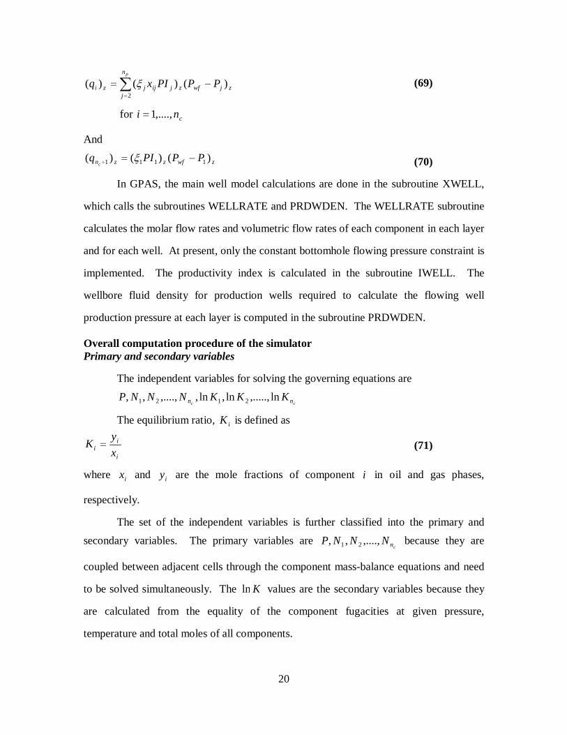
pn

jzjwfzjijjzi PPPIxq

2)()()( �

for cni ,....,1�

(69)

And

zwfzzn PPPIqc

)()()( 1111 ��

� (70)

In GPAS, the main well model calculations are done in the subroutine XWELL,

which calls the subroutines WELLRATE and PRDWDEN. The WELLRATE subroutine

calculates the molar flow rates and volumetric flow rates of each component in each layer

and for each well. At present, only the constant bottomhole flowing pressure constraint is

implemented. The productivity index is calculated in the subroutine IWELL. The

wellbore fluid density for production wells required to calculate the flowing well

production pressure at each layer is computed in the subroutine PRDWDEN.

Overall computation procedure of the simulatorPrimary and secondary variables

The independent variables for solving the governing equations are

cc nn KKKNNNP ln,.....,ln,ln,,....,,, 2121

The equilibrium ratio, iK is defined as

i

ii x

yK � (71)

where ix and iy are the mole fractions of component i in oil and gas phases,

respectively.

The set of the independent variables is further classified into the primary and

secondary variables. The primary variables are cnNNNP ,....,,, 21 because they are

coupled between adjacent cells through the component mass-balance equations and need

to be solved simultaneously. The Kln values are the secondary variables because they

are calculated from the equality of the component fugacities at given pressure,

temperature and total moles of all components.

21

Solution procedure

A fully implicit solution method is used to solve the governing equations. The

equations are nonlinear and must be solved iteratively. A Newton procedure is used in

which the system of nonlinear equations is approximated by a system of linear equations.

The Jacobian term refers to the matrix whose elements are the derivatives of the

governing equations with respect to the independent variables.

The sequence of steps involved in the solution of the governing equations for the

independent variables over a timestep include:

1. Initialization in each gridblock : The Pressure, overall composition and

temperature of the fluids in each gridblock are specified.

The initialization and calculation of the initial fluid in place is done in the

subroutine INFLUID0. This subroutine is the main driver for the

computation of the initial fluid in place.

2. Phase identification and Physical properties calculation: The flash

calculations are performed in each gridblock and the phase saturations,

compositions and densities are determined. The phases are then

identified as gas, oil or aqueous phase. Phase viscosities and relative

permeabilities are subsequently computed. The flash calculations are

performed in the subroutine XFLASH and currently are limited to two

phases. The Rachford-Rice equation that determines the phase fractions

is coded in the subroutine SOLVE. All the fluid physical properties like

the fluid viscosity, relative permeability and phase density calculations

are determined in the PROP subroutine. The PROP subroutine calls

separate routines to determine the different physical properties. It calls

the subroutine LVISC2 to calculate the phase viscosity using the Lorenz

coefficient, the subroutine RELPERM3EOS to calculate the three-phase

relative permeability using Stone's model or calls the LOOKUP

22

subroutine to interpret the two-phase relative permeability from the

relative permeability tables.

3. Governing Equations Linearization. All the governing equations are

linearized in terms of the independent variables and the elements of the

Jacobian are calculated.

The subroutine JACOBIAN that in turn calls PREROW generates the

Jacobian for the linear system. PREROW is the main subroutine that calls

the other subroutines, each with a specific task of computing the

derivatives of separate equations and terms. The subroutine JACCUM

calculates the derivatives of the accumulation term of the component

balance. The subroutine JACO2 calculates the derivatives related to

transmissibility terms. The subroutine JMASS calculates the derivatives

related to the component mass balance in X, Y and Z directions. The

derivatives of the source/sink terms are calculated in JSOURCE.

4. Jacobian Factorization and reduction of the linear systems. A row

elimination is performed to reduce the size of the linear system from

12 �cn to cn for each gridblock. To achieve this, the linearized phase-

equilibrium relations and the linearized volume constraint are used to

eliminate the secondary variables and one of the overall component

moles from the linearized component mass balance equations.

The subroutine EOS_JACO forms the jacobian for row elimination for

two-phase cells.

5. Solution of the reduced system of the linear equations for the primary

variables. The reduced system of linear equations is simultaneously

solved for pressure and the overall moles of 1�cn components per unit

bulk volume for all the cells.

6. Secondary variables calculation. A back substitution method is

23

employed to compute the secondary variables Kln and overall moles of

the component eliminated in Step 4 using the factorized Jacobian. The

phase-stability analysis is then carried out for all the gridblocks using the

newly updated pressure and overall component moles.

7. Updating phase densities and viscosities, determination of single-phase

state and estimation of phase relative permeability.

The subroutine XUPDATE updates the phase composition and the phase

properties as phase density, viscosity, relative permeability and

determination of single phase in each cell. The main subroutine in the

compositional model EOSCOMP is XSTEP. XSTEP calls XDELTA,

which in turn calls the XUPDATE subroutine.

8. Check for convergence. The residuals of the linear system obtained in

step 3 are used to determine convergence. If a tolerance is exceeded, the

elements of the Jacobian and the residuals of the governing equations are

then updated and another Newton iteration is performed by returning to

Step 4. If the tolerance is met, a new timestep is then started by returning

to Step 3.

The subroutine XSTEP is the contact routine between the IPARS

framework code and the EOSCOMP compositional model code. The

residuals are checked in XSTEP and if the tolerance is met, a new

timestep is started, else another newton iteration is performed.

Executive routines in EOSCOMP

The executive routines in the EOSCOMP model are as follows:

XISDAT All the initial scalar data are read by this subroutine. These

include the physical properties of each component, default

number of iterations, convergence tolerances for a variety of

24

calculations, output flags, operation specific flags and chemical

property data. No grid-element arrays can be reference in this

subroutine.

XARRAY This subroutine allocates memory for all the grid element

arrays

XIADAT The entire grid element array input as the pressure, water

saturation, feed composition is read in and written out to a file

XIVDAT. Performs the model initialization before time iteration. The

PETSc linear solver is also initialized.

XSTEP The main subroutine that performs all the calculations over a

timestep.

XQUIT Exits from the simulation when it meets the maximum time,

production limits, or if an error occurs.

The communication between processors for the compositional model is performed

in the executive subroutines. There is no argument attached to these calls. Those

variables associated with grids are passed into these routines through pointers that are

stored in common block. These common blocks are included as header files in the

subroutines. The executive routines call the work routines to perform all the calculations.

The grid dimensions and variables are passed into these work routines through a C

routine called CALLWORK, which is handled by the framework. The CALLWORK

function passes the variables as an index argument list to the function being called.

Description of the Solver

PETSc (Balay et al., 1997, 1998; Wang et al., 1999) is a large suite of parallel,

general-purpose, object-oriented solvers for the scalable solution of partial differential

equations discretized using implicit and semi-implicit methods. PETSc is implemented in

C, and is usable from C, Fortran, and C++. It uses MPI for communication across

25

processors. GPAS uses the linear solver component of PETSc to solve the linearized

Newton system of equations and uses the parallel data formats provided by PETSc to

store the Jacobian and the vectors.

The linear solver components of PETSc provides a unified interface to various

Krylov methods, such as conjugate gradient (CG), generalized minimal residual

(GMRES), biconjugate gradient, etc. and also to various parallel preconditioners such as

Jacobi, block preconditioners like block Jacobi, domain decomposition preconditioners

like additive Schwartz. GPAS uses the biconjugate gradient stabilized approach as the

Krylov method and block Jacobi preconditioner, with point block incomplete

factorization (ILU) on the subdomain blocks. The point block refers to treating all the

variables associated with a single gridblock as a single unit. The number of subdomain

blocks for block Jacobi is chosen to match the number of processors used, so that each

processor gets a complete subdomain of the problem and does a single local incomplete

factorization on the Jacobian corresponding to this subdomain.

For three-phase flow, the compositional model. EOSCOMP generates 12 �cn

equations per gridblock, causing the Jacobian to have a point-block structure and a point-

block sparse storage format is used to store the matrix. These 12 �cn equations do not

result in complete coupling of all the variables across gridblocks. This causes the

Jacobian to have some 1�cn point-block locations with zero values. Thus a block size of

1�cn is chosen for this matrix type eliminating the need to store the � �1�cn � �1�cn

blocks with zero values. The usage of the point-block sparse matrix storage lead to the

improvement in the performance of the matrix routines.

26

Task 2: Formulation and Implementation of Chemical Module

The first set of chemical species added to the GPAS simulator is the tracer. Thus,

although all the formulation in the aqueous species modeling applies to tracer, polymer

and surfactant, each of these species modeling can involve, in addition, its own

assumptions, formulations and special properties. Henceforth, the aqueous species refers

to a species present in trace quantities in the aqueous phase and this includes a tracer,

polymer or surfactant, the main subroutine XAQCOMP solving for the aqueous species

concentration as a function of space and time is referred as the chemical subroutine and

the whole module encompassing all the separate subroutines modeling the tracer,

polymer and surfactant features is referred as the chemical module. The final output of

the chemical subroutine XAQCOMP is the dimensionless aqueous species concentration,

which also applies as the physical tracer concentration.

In GPAS simulator, the chemical module was linked to the equation-of-state

compositional model EOSCOMP in an explicit manner. After EOSCOMP solves for the

pressures, saturations and compositions of the non-aqueous species components for a

particular time step and the convergence for the mass balance equations is attained, the

chemical subroutine imports the required input from the host EOSCOMP and solves for

the aqueous species mass balance equation to find the concentration at a given point in

space and time.

This decoupled approach is more computationally efficient than solving all of the

equations simultaneously in EOSCOMP.

Maroongroge (1994) used the following approach for tracer calculations in

UTCOMP:

� Solution of the pressure equation.

� Solution of the mass conservation equations for species other than tracers

27

� Flash calculation to calculate the phase compositions of species other than

tracers.

� Computation of the phase densities, saturations, relative permeabilities,

and capillary pressures.

� Solution of the mass conservation equations for tracer components from

the independent variables. This includes the re-determination of the

upstream locations from the potentials, the calculation of the convection

terms from the transmissibility coefficients, phase mole fractions, densities

and fluxes, and the recalculation of the well flow rates in each layer.

� Return to the first step, the solution of the pressure equation for a new

time step.

In GPAS, the parameters such as the phase flux, phase saturation, phase density

and upstream locations are already being calculated in EOSCOMP. Because the aqueous

species do not alter the phase behavior, the equation-of-state flash calculations are

performed only for the non-aqueous species and subsequently the phase saturations,

phase densities and phase fluxes are determined. In order to make the code efficient,

these fluid flow and rock parameters were transferred from EOSCOMP at the last

Newtonian iteration of each timestep to the chemical subroutine. The grid-block

pressures are no longer required as the other parameters have already accounted for the

pressure term.

The simplified method used in GPAS is as follows:

� Transfer of phase saturations, phase densities, phase flux, upstream

locations and the well molar flow rates from EOSCOMP to the chemical

subroutine.

� Solution of the mass conservation equation for the aqueous species

incorporating the convection terms and the source/sink terms.

� Return to Step 1 for a new time step

28

A notable feature of this method is that the chemical module calculations are not

performed for each Newtonian iteration in a timestep, since the equations for aqueous

species flow are decoupled and can be solved explicitly. This saves considerable

computing time for reservoir simulations with a large number of gridblocks.

Mathematical formulation

Aqueous Species Mass Conservation Equation

The differential form for the species mass conservation equation is expressed as:

NciR

KSuSt

i

Np

jijijsjjijj

Np

jissijjj

,..,1,

)()1(11

��

��

��

��

��

��

��

�

��

�� (2.1)

where j� is the mass density of phase j , jS is the saturation of phase j , ij� is the mass

fraction of species i in j , s� is the mass density of the stationary phase s , ijK is the

dispersion tensor, is� is the mass fraction of species i in the stationary phase s , ju is the

flux of phase j , and iR is the source/sink term.

The species mass conservation equation was simplified to model the aqueous

species flow using the below assumptions:

� Aqueous species do not occupy any volume

� Physical dispersion is neglected.

� Radioactive decay does not occur

� Aqueous species stay in the aqueous phase and do not partition to the oil

or gas phase.

The additional specific assumptions that apply only to a physical tracer are

� Tracers do not change the physical properties of the fluids.

� Tracer adsorption does not take place

� Tracers do not undergo chemical reactions

29

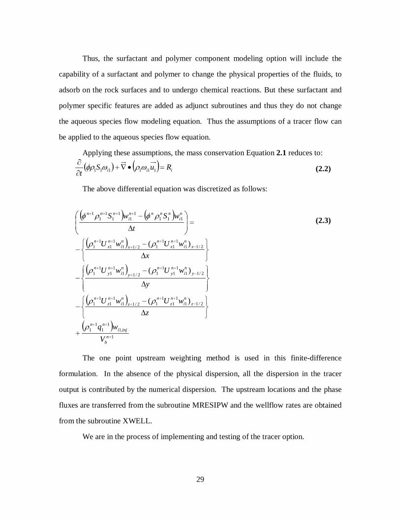
Thus, the surfactant and polymer component modeling option will include the

capability of a surfactant and polymer to change the physical properties of the fluids, to

adsorb on the rock surfaces and to undergo chemical reactions. But these surfactant and

polymer specific features are added as adjunct subroutines and thus they do not change

the aqueous species flow modeling equation. Thus the assumptions of a tracer flow can

be applied to the aqueous species flow equation.

Applying these assumptions, the mass conservation Equation 2.1 reduces to:

� � � � iii RuSt

��

�111111 �� (2.2)

The above differential equation was discretized as follows:

� � � �

� �

� �

� �

� �1

,11

11

1

2/111

11

12/111

11

1

2/111

11

12/111

11

1

2/111

11

12/111

11

1

1111

11

11

11

)(

)(

)(

�

��

�

��

�

��

�

��

�

��

�

��

�

��

��

�

��

��

�

�

��

�

��

�

��

��

�

��

�

��

�

�

�

nb

injinn

zni

nz

nz

ni

nz

n

yni

ny

ny

ni

ny

n

xni

nx

nx

ni

nx

n

ni

nnnni

nnn

Vwq

zwUwU

y

wUwU

xwUwU

twSwS

�

��

��

��

�� (2.3)

The one point upstream weighting method is used in this finite-difference

formulation. In the absence of the physical dispersion, all the dispersion in the tracer

output is contributed by the numerical dispersion. The upstream locations and the phase

fluxes are transferred from the subroutine MRESIPW and the wellflow rates are obtained

from the subroutine XWELL.

We are in the process of implementing and testing of the tracer option.

30

Task 3: Validation and Application

Test cases were run on GPAS and the results were compared with both analytical

solutions and output from the miscible-gas flooding compositional simulator, UTCOMP

(Chang, 1990), or the chemical flooding simulator, UTCHEM (Delshad et al., 1996), to

check the correctness of the code. The flash algorithm was tested with a batch flash

calculation for a binary mixture. A Buckley-Leverett problem was run on GPAS and

compared with the analytical solution and output from the chemical flooding simulator

UTCHEM. A comparison of the results from GPAS with UTCOMP of an example

simulation of carbon dioxide sequestration is also given. The standard SPE fifth

comparative solution project (Killough and Kossack, 1987) was modified and simulations

were carried out on GPAS and UTCOMP. The comparison of these results from GPAS

with UTCOMP for the modified SPE fifth comparative solution project is discussed.

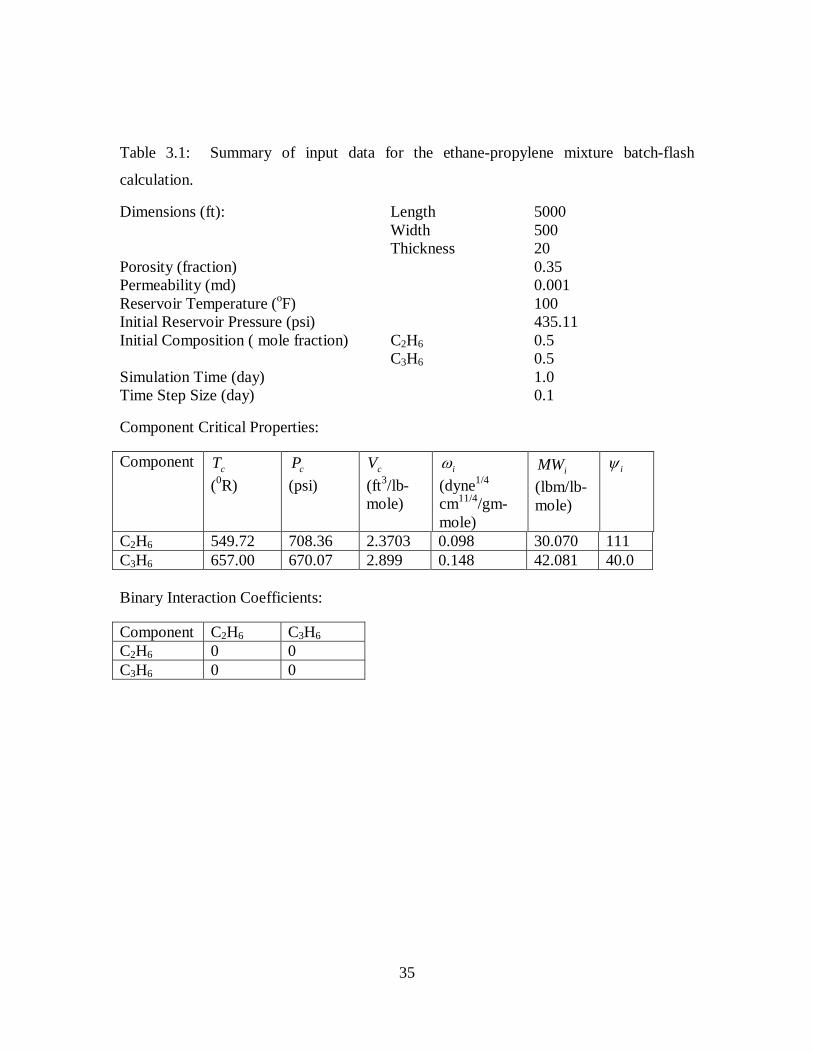
Batch flash of Ethane-Propylene binary mixture

The goal is to verify the correctness of the flash calculations. The mathematical

formulation of the flash algorithm is discussed in Task 1. The test case considered here is

a mixture of ethane and propylene. The simulation domain dimensions are 5000 ft in

length, 500 ft in width and 20 ft in thickness. Since the simulation is a batch flash, there

is no well section in the input. The initial composition is 0.5 mole fraction each of ethane

and propylene. The details of the input file including the critical properties of the

components are given in Table 3.1. The simulation is run for one day. A program for

multi-component vapor-liquid equilibrium calculations using the Peng-Robinson cubic

equation-of-state, VLMU (Sandler, 1999) was also used as a basis for comparison.

UTCOMP and GPAS use the same form of PR EOS while VLMU uses a slightly

different form of PR EOS. For acentric factor values less than 0.49, all the three codes

use the same equations. The only difference is that GPAS and UTCOMP use a different

expression for the calculation of � (Equation 29) for the acentric factor values greater

31

than 0.49 while VLMU uses the same expression for all values of acentric factors

(Equation 28). Since in this test case, the acentric factor for both the components is less

than 0.49, all the three codes essentially use the same PR EOS equations. The iteration

tolerances in UTCOMP and GPAS are set at 10-8. The volume shift parameter

functionality is available in UTCOMP but is not implemented in GPAS and VLMU.

Hence the volume shift parameter is taken as zero in UTCOMP.

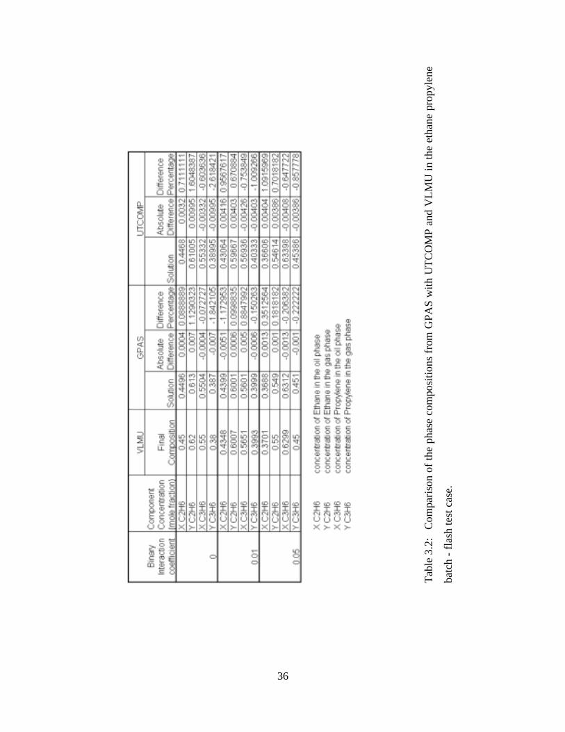
Changing the binary interaction coefficient to 0, 0.01 and 0.05, three simulation

runs were made. The oil and gas phase compositions from GPAS, UTCOMP and VLMU

are compared in Table 3.2. The differences in the concentrations were based on VLMU

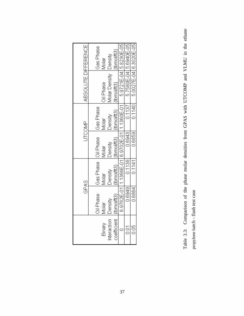
solution. The oil and gas phase molar densities obtained from GPAS and UTCOMP are

compared in Table 3.3. A reasonable agreement was obtained for the flash calculation

results between GPAS and UTCOMP.

Buckley Leverett 1-D water flood

The Buckley-Leverett problem was chosen as a test problem because there is an

analytical solution available for comparison. This problem often serves as a test for new

numerical methods and as a building block of simulation models involving simultaneous

flow of immiscible fluids in porous media.

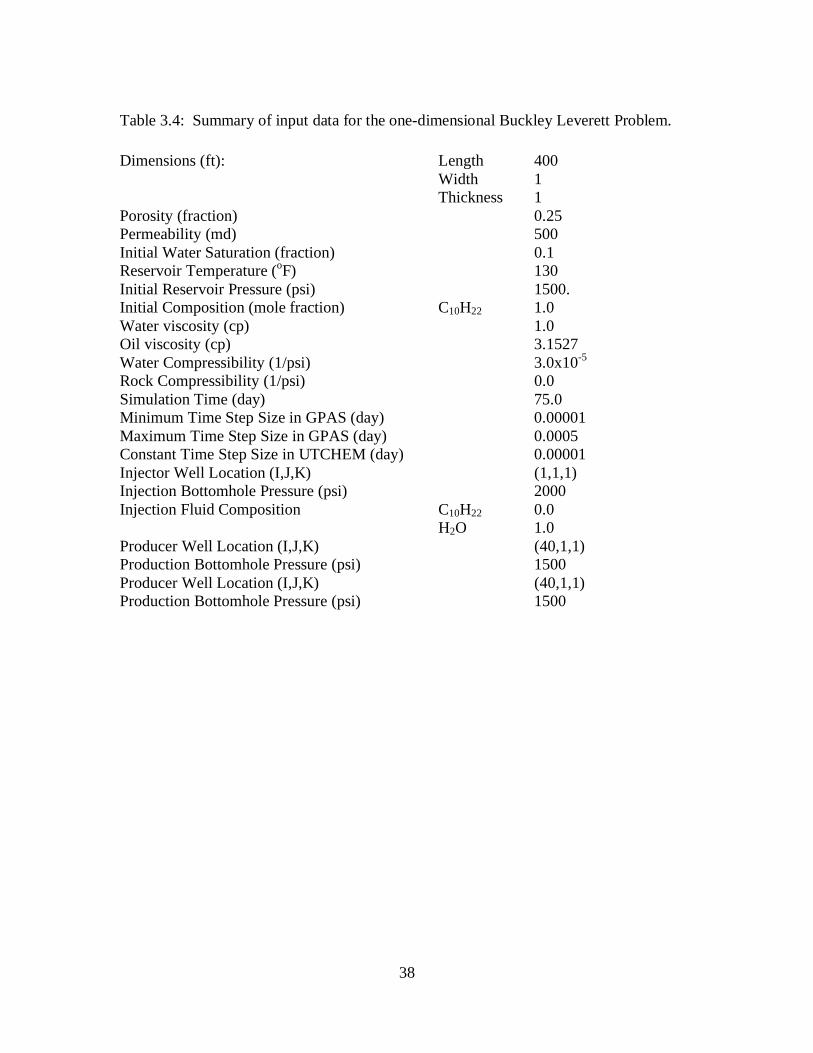
The problem considered is a one-dimensional waterflood in a gas free,

homogenous, isotropic reservoir. The homogenous permeability is 500 md. The

simulation domain extends to 400 ft in the x direction, 1 ft in the y direction and 1 ft in

the z direction. A 40x1x1 grid was used for this run. The initial water saturation in the

reservoir is 0.1. The only injector is located at gridblock (1,1,1) and the only producer is

located at gridblock (40,1,1). The initial reservoir pressure is 1500 psia. Water is injected

at a constant bottom hole pressure of 2000 psia and the producer is maintained at a

constant bottom hole pressure of 1500 psia. The relative permeability curves used for

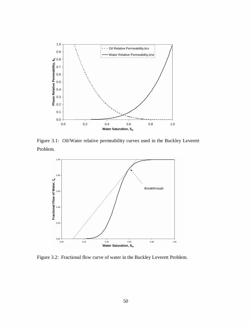
this problem are shown in Figure 3.1. The two-phase relative permeability tables, used

32

in GPAS, were generated based on these functions. The end point mobility ratio is 3.15.

The reservoir description, the hydrocarbon component properties and the time step details

of the input file are given in Table 3.4. The fractional flow curves of oil and water are

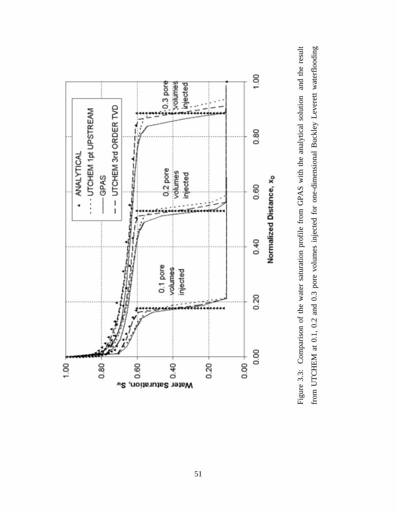
presented in Figure 3.2. The water saturation profile results from GPAS, at different

injected pore volumes, was compared with the output from UTCHEM and the analytical

solution in Figure 3.3 The one-point upstream weighting numerical method is employed

for this simulation in GPAS, while both one point upstream and third order TVD (total

variation diminishing) methods are employed in UTCHEM. A constant time step of 0.1

days in used in UTCHEM while in GPAS the maximum time step is 0.0005 days and the

minimum time step is 0.00001 days. When the third order TVD numerical method (total

variation diminishing) is used in UTCHEM, its results are closer to the analytical solution

than when the one point upstream weighing method is used.

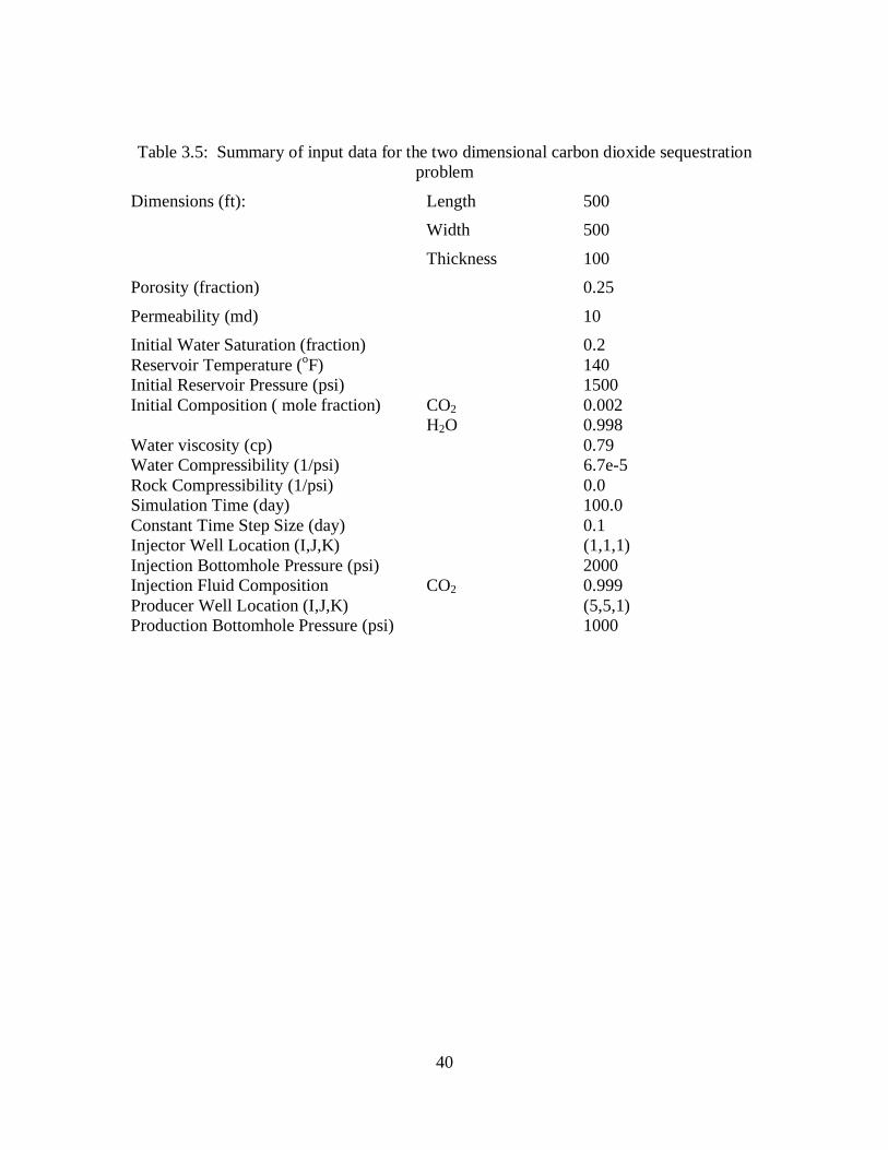
Carbon dioxide sequestration case

The injection of carbon dioxide into a two-dimensional, isotropic, homogenous

aquifer was simulated. After making the simulations with GPAS and UTCOMP, the

pressure, saturation and composition profiles were compared.

The simulation domain is 500 ft in length, 500 ft in width and 100 ft in thickness.

A 5x5x1 grid was used for this simulation. Water is treated here as a component so that

the solubility of the carbon dioxide in the liquid water phase can be calculated from the

equation-of-state. Phase 2 is the active liquid water phase and phase 3 is the gas phase in

these simulations. The usual water phase is 1, but it plays no significant role in these

simulations. Its saturation was a constant equal to 0.2. Carbon dioxide is injected into

the aquifer through the injector located at gridblock (1,1,1) at a bottom hole pressure of

2000 psi. The producer well is located at gridblock (5,5,1) with a constant bottom hole

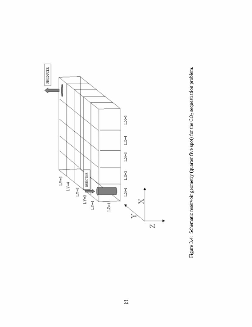
pressure of 1000 psi. The initial reservoir pressure is 1500 psi. Figure 3.4 shows a

diagram of the reservoir. A summary of the input data is given in Table 3.5.

33

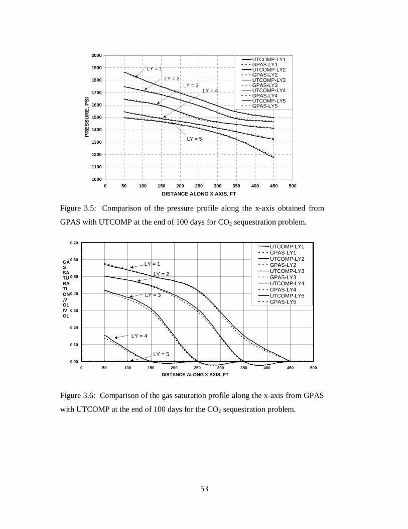
The simulation is carried out for 100 days and the pressure, the saturation and

composition profiles at the end of 100 days compared with good agreement. The

pressure profile along the x-axis has been plotted for every Y index in Figure 3.5. The

gas saturation profile along the x-axis was plotted for every Y grid index in Figure 3.6.

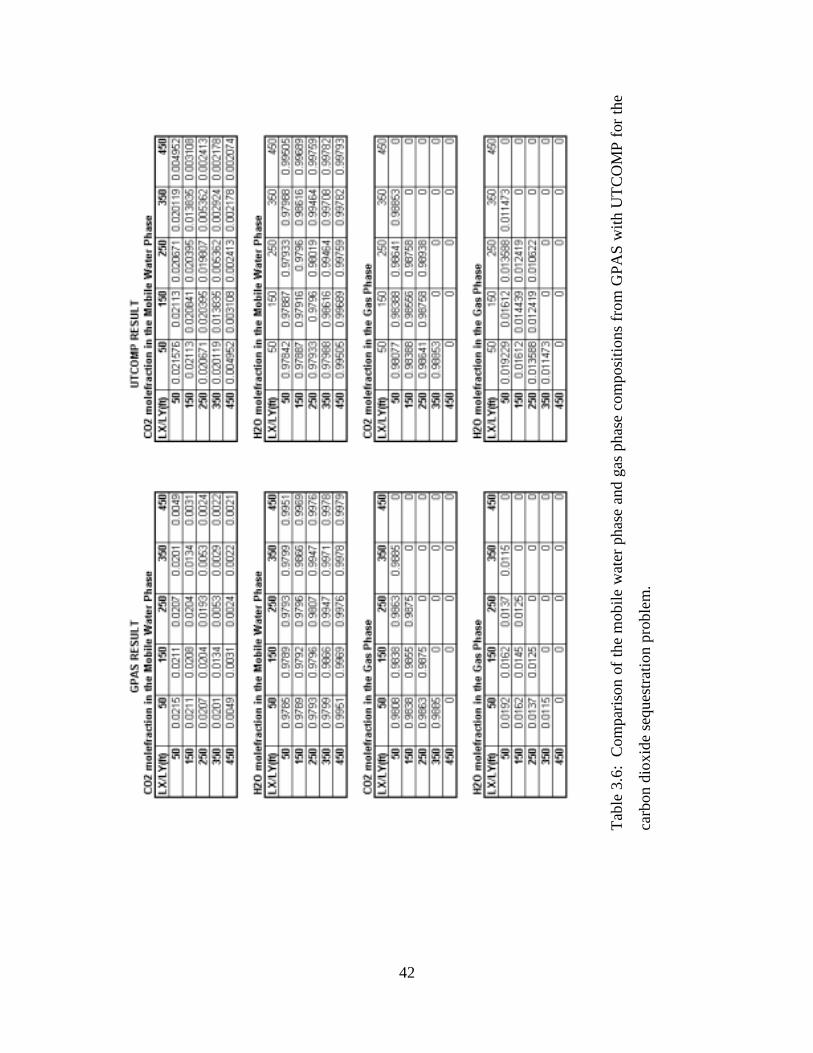
The compositions of the water phase and the gaseous phase at the end of 100 days from

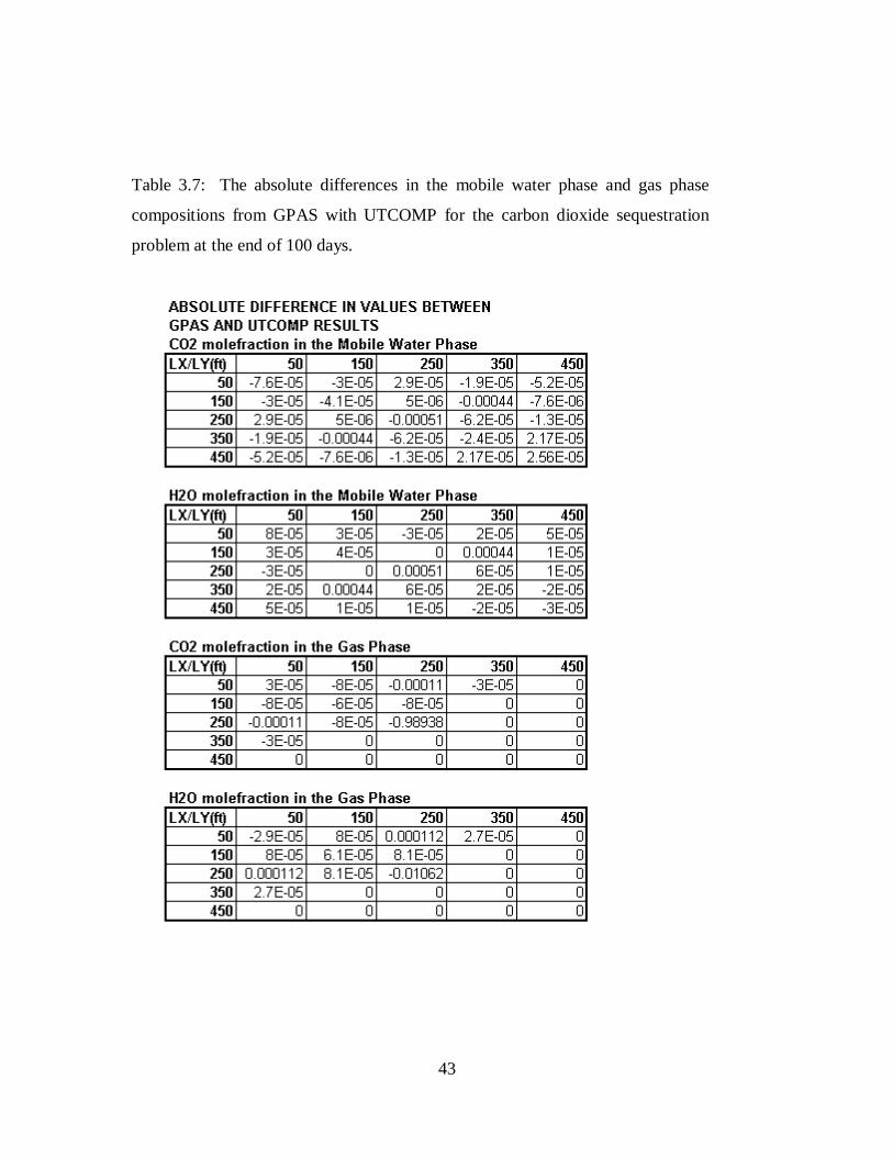
GPAS and UTCOMP are given in Table 3.6. The absolute differences between the

compositions obtained from GPAS and UTCOMP at the end of 100 days are given in

Table 3.7.

Six-Component compositional simulation example

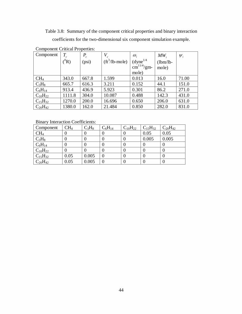
This test is a modified version of the SPE fifth comparative solution problem.

The hydrocarbon phase consists of six components. The hydrocarbon component critical

properties are given in Table 3.8. Two-dimensional and three-dimensional simulations

of the same problem were run to verify the correctness of the two- and three-dimensional

features of the simulator.

Two Dimensional Quarter Five Spot Case

A quarter five spot pattern (5x5x1) is used for this run. The reservoir description

and the well constraints are presented in Table 3.9. The simulation domain comprises of

500 ft in the x direction, 500 ft in the y direction and 100 ft in the z direction. The

injector well is located at (1,1,1) and the producer well is located at (5,5,1). Gas is

injected into the reservoir and it pushes the oil towards the producer. The water phase is

immobile. The pressure profile and the saturation profile at the end of 100 days obtained

from GPAS and UTCOMP was compared and a good agreement was obtained. The

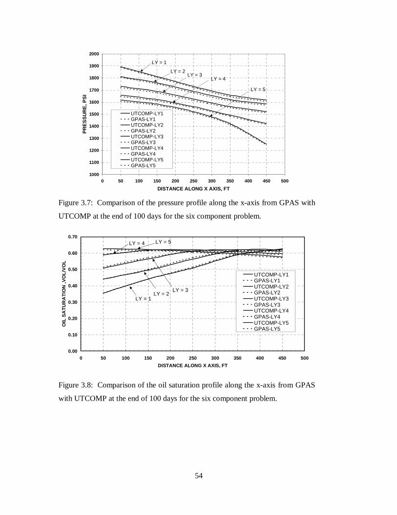
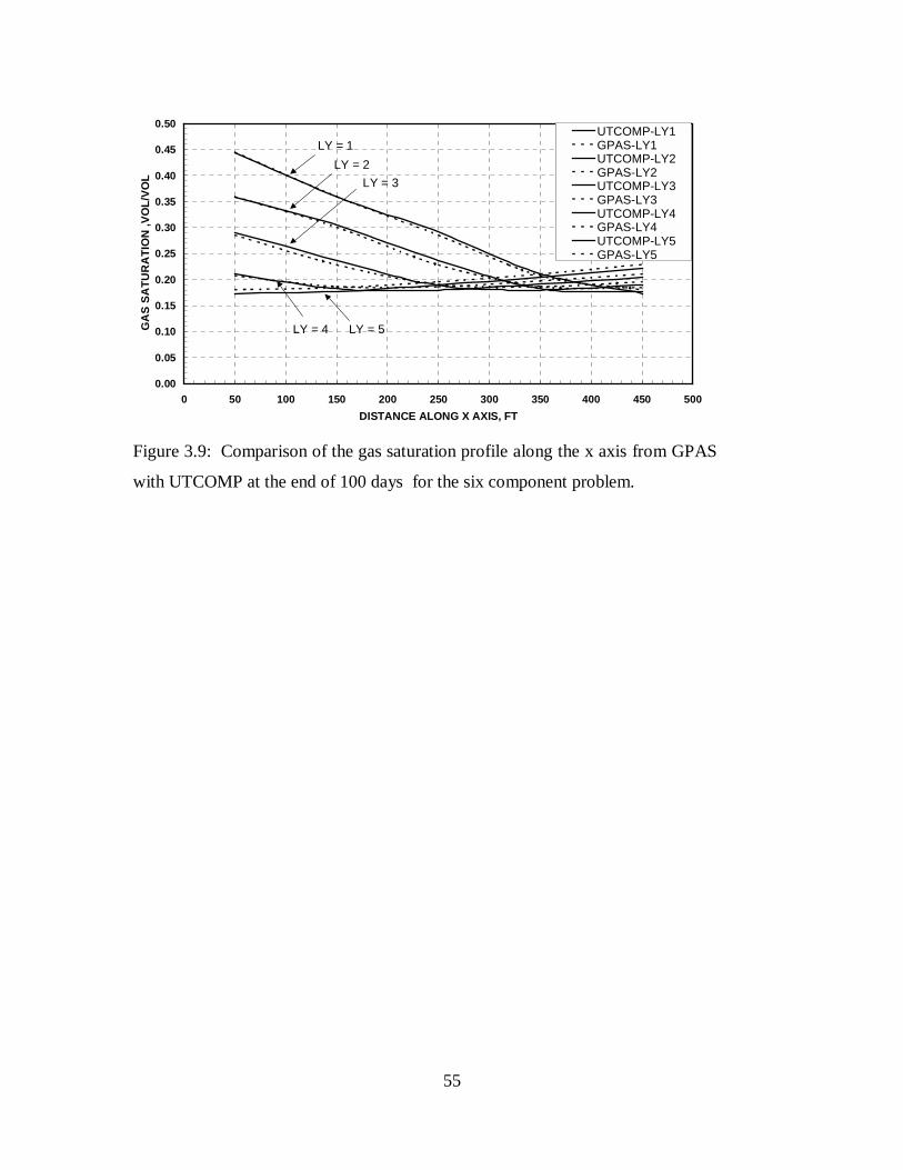
pressure profile along the x-axis has been plotted for every Y index in Figure 3.7. The

oil saturation profile and the gas saturation profile along the x-axis for every y index is

plotted in Figure 3.8 and Figure 3.9 respectively and as shown there is a reasonably

34

good agreement obtained between the two simulator results. This supports the

correctness of the two dimensional three phase compositional capabilities of GPAS.

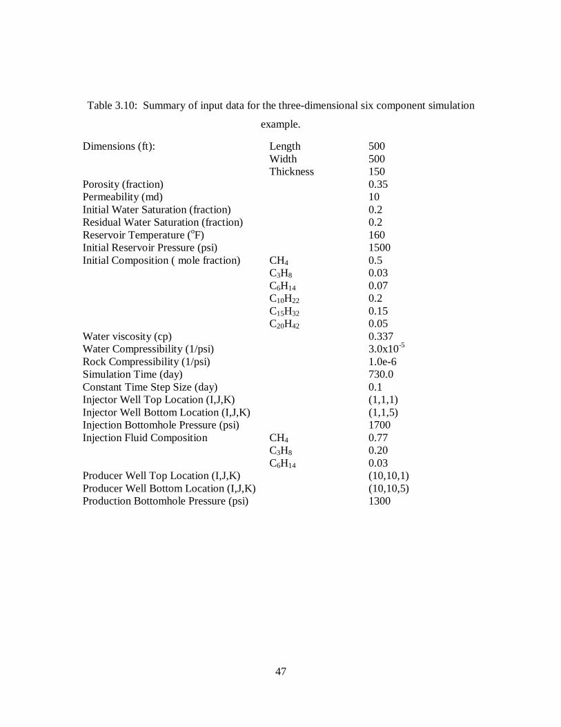
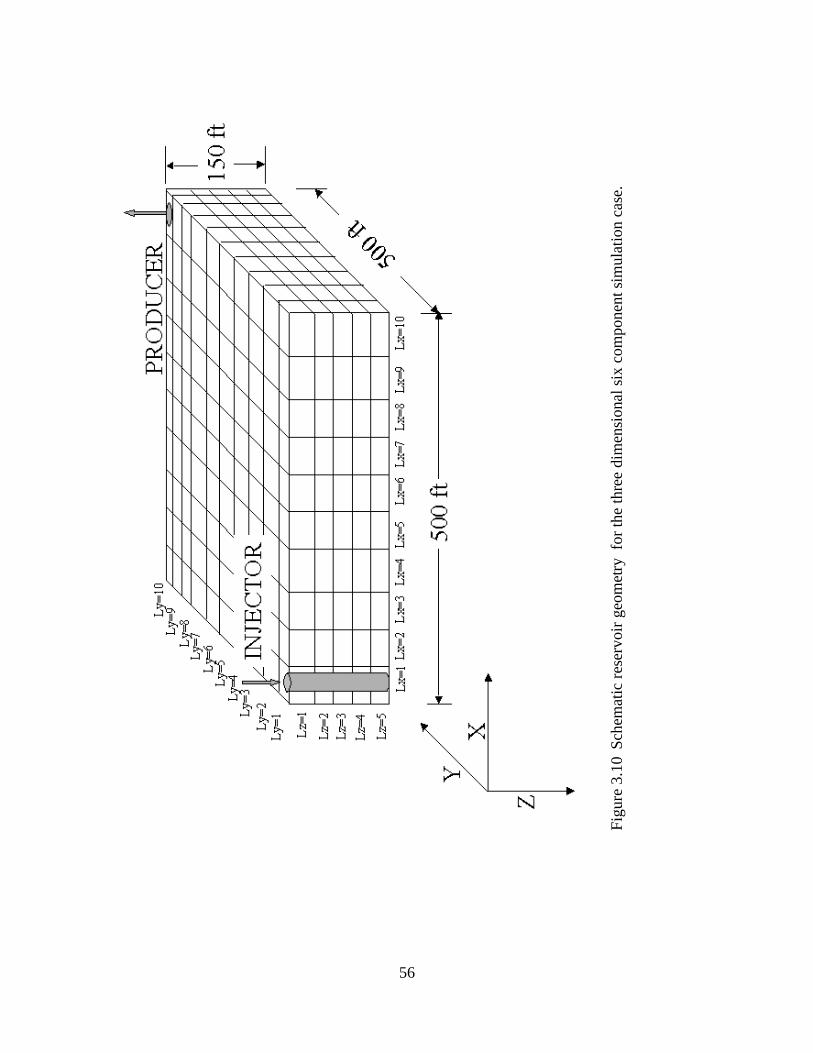
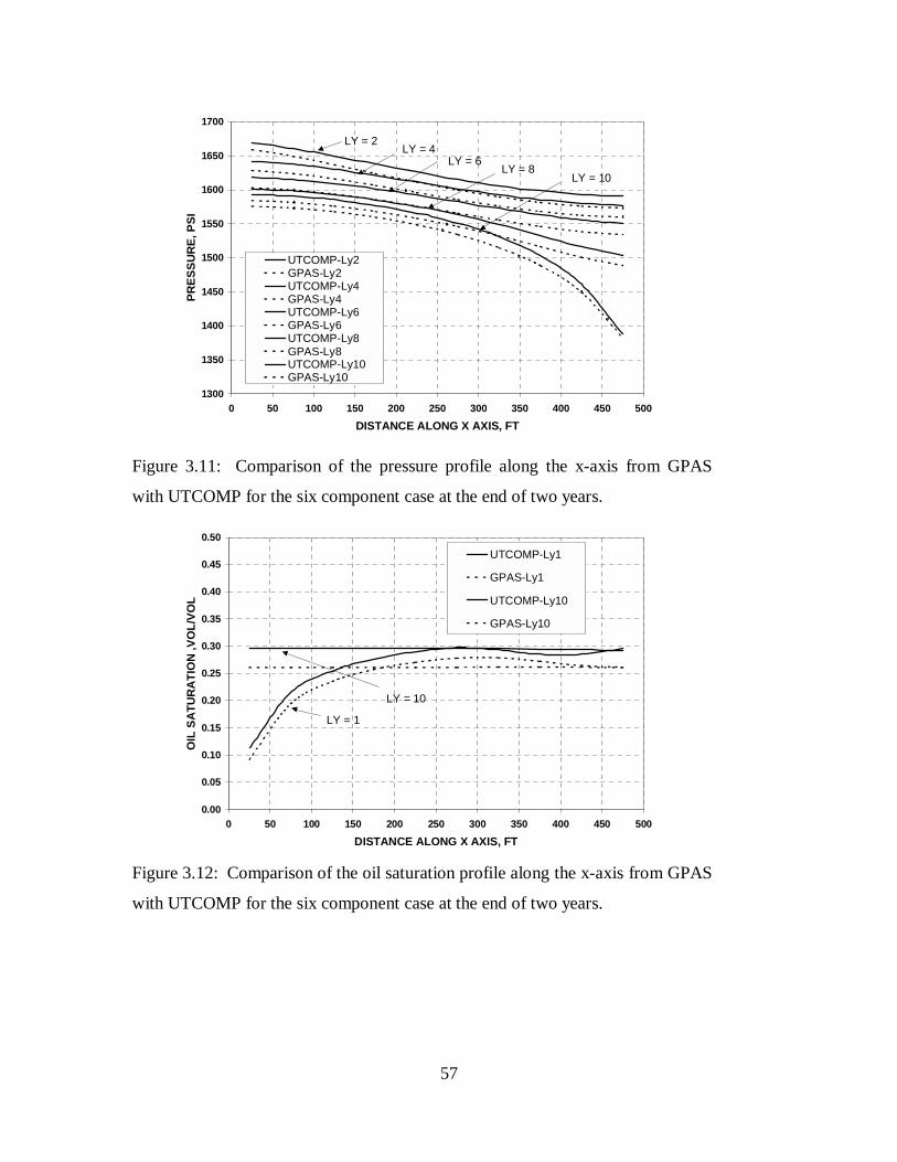
Three Dimensional Case

A 10x10x5 finite difference grid was used as shown in Figure 3.10. The input

data summary for this run is given in Table 3.10. The critical properties and the binary

interaction coefficients are given in Table 3.8. The injector well and the producer well

are completed through all the five layers. The injector is located at (1,1) and the producer

well is located at (10,10). Gas is continuously injected at a constant bottomhole pressure

of 1700 psi and the producer well is constantly maintained at 1300 psi. The initial

reservoir pressure is 1500 psi. The water phase is immobile. The test case is run on

GPAS and UTCOMP for a simulation period of two years. The pressure distribution,

fluid saturations and concentrations from GPAS compared well with UTCOMP. The

plots of the pressure profile along the x axis for the even grid index in the Y direction and

only for the top layer at the end of two years is plotted in Figure 3.11. The oil saturation

profile and the gas saturation profile along the x-axis, only for the extreme Y grid index

in the top layer and at the end of two years, from GPAS and UTCOMP were compared in

Figure 3.12 and Figure 3.13 respectively. The average reservoir pressure history from

GPAS and UTCOMP were compared in Figure 3.14. The overall production gas oil

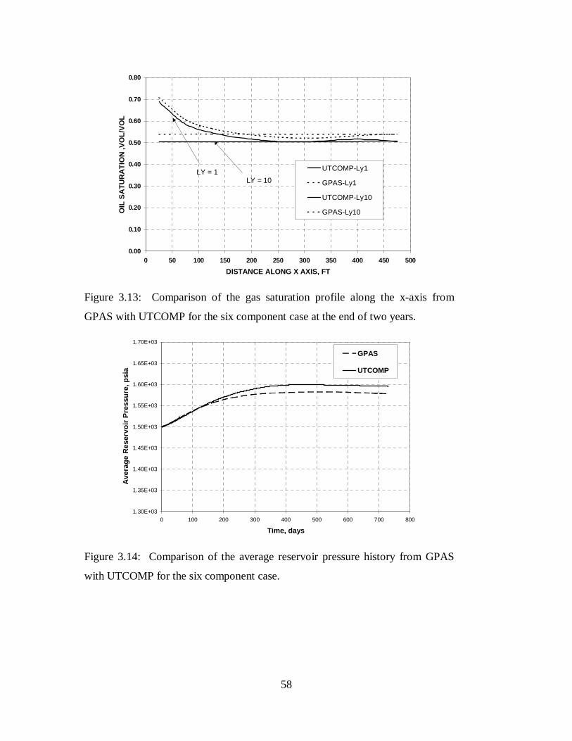
ratio comparison plots are shown in Figure 3.15.

35

Table 3.1: Summary of input data for the ethane-propylene mixture batch-flash

calculation.

Dimensions (ft): Length 5000Width 500Thickness 20

Porosity (fraction) 0.35Permeability (md) 0.001Reservoir Temperature (oF) 100Initial Reservoir Pressure (psi) 435.11Initial Composition ( mole fraction) C2H6 0.5

C3H6 0.5Simulation Time (day) 1.0Time Step Size (day) 0.1

Component Critical Properties:

Component cT(0R)

cP(psi)

cV(ft3/lb-mole)

i�

(dyne1/4

cm11/4/gm-mole)

iMW(lbm/lb-mole)

i�

C2H6 549.72 708.36 2.3703 0.098 30.070 111C3H6 657.00 670.07 2.899 0.148 42.081 40.0

Binary Interaction Coefficients:

Component C2H6 C3H6C2H6 0 0C3H6 0 0

36

Tabl

e 3.

2:

Com

paris

on o

f the

pha

se c

ompo

sitio

ns fr

om G

PAS

with

UTC

OM

P an

d V

LMU

in th

e et

hane

pro

pyle

ne

batc

h - f

lash

test

cas

e.

37

Tabl

e 3.

3:

Com

paris

on o

f th

e ph

ase

mol

ar d

ensi

ties

from

GPA

S w

ith U

TCO

MP

and

VLM

U i

n th

e et

hane

prop

ylen

e ba

tch

- fla

sh te

st c

ase

38

Table 3.4: Summary of input data for the one-dimensional Buckley Leverett Problem.


Porosity (fraction) 0.25Permeability (md) 500Initial Water Saturation (fraction) 0.1Reservoir Temperature (oF) 130Initial Reservoir Pressure (psi) 1500.Initial Composition (mole fraction) C10H22 1.0Water viscosity (cp) 1.0Oil viscosity (cp) 3.1527Water Compressibility (1/psi) 3.0x10-5

Rock Compressibility (1/psi) 0.0Simulation Time (day) 75.0Minimum Time Step Size in GPAS (day) 0.00001Maximum Time Step Size in GPAS (day) 0.0005Constant Time Step Size in UTCHEM (day) 0.00001Injector Well Location (I,J,K) (1,1,1)Injection Bottomhole Pressure (psi) 2000Injection Fluid Composition C10H22 0.0

H2O 1.0Producer Well Location (I,J,K) (40,1,1)Production Bottomhole Pressure (psi) 1500Producer Well Location (I,J,K) (40,1,1)Production Bottomhole Pressure (psi) 1500

39

Table 3.4 (Cont.)

Component Critical Properties:Component cT

(0R)cP

(psi)cV

(ft3/lb-mole)

i�

(dyne1/4

cm11/4/gm-mole)

iMW(lbm/lb-mole)

i�

C10H22 1111.8 304.0 12.087 0.488 142.3 431.0

Relative Permeability functions used for generating the tables

1.04

101

�

�

�

wr

r

SmK

04

102

�

�

�

or

r

SnK

� �morr

wror

wrw

SKK

SSSSS

11

1

�

��

�

� � �norr SKK �� 122

40

Table 3.5: Summary of input data for the two dimensional carbon dioxide sequestrationproblem

Dimensions (ft): Length 500

Width 500

Thickness 100

Porosity (fraction) 0.25

Permeability (md) 10

Initial Water Saturation (fraction) 0.2Reservoir Temperature (oF) 140Initial Reservoir Pressure (psi) 1500Initial Composition ( mole fraction) CO2 0.002

H2O 0.998Water viscosity (cp) 0.79Water Compressibility (1/psi) 6.7e-5Rock Compressibility (1/psi) 0.0Simulation Time (day) 100.0Constant Time Step Size (day) 0.1Injector Well Location (I,J,K) (1,1,1)Injection Bottomhole Pressure (psi) 2000Injection Fluid Composition CO2 0.999Producer Well Location (I,J,K) (5,5,1)Production Bottomhole Pressure (psi) 1000

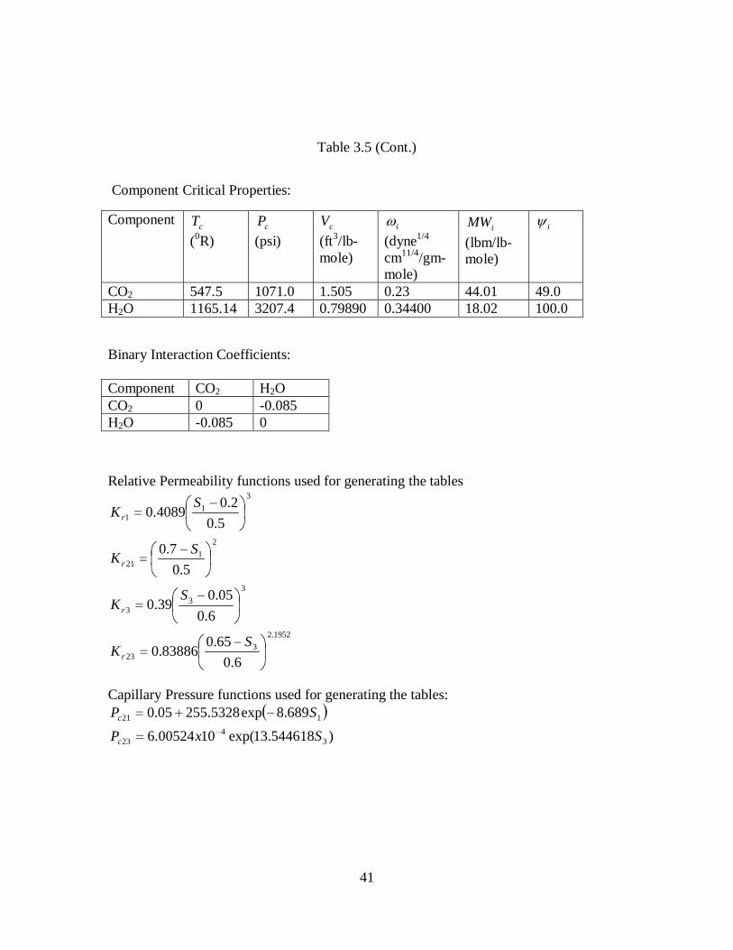
41

Table 3.5 (Cont.)

Component Critical Properties:

Component cT(0R)

cP(psi)

cV(ft3/lb-mole)

i�

(dyne1/4

cm11/4/gm-mole)

iMW(lbm/lb-mole)

i�

CO2 547.5 1071.0 1.505 0.23 44.01 49.0H2O 1165.14 3207.4 0.79890 0.34400 18.02 100.0

Binary Interaction Coefficients:

Component CO2 H2OCO2 0 -0.085H2O -0.085 0


1952.23

23

33

3

21

21

31

1

6.065.0

83886.0

6.005.0

39.0

5.07.0

5.02.0

4089.0

��

��

� ��

��

��

� ��

��

��

� ��

��

��

� ��

SK

SK

SK

SK

r

r

r

r

Capillary Pressure functions used for generating the tables:� �

)544618.13exp(1000524.6689.8exp5328.25505.0

34

23

121

SxPSP

c

c�

�

��

42

Tabl

e 3.

6: C

ompa

rison

of t

he m

obile

wat

er p

hase

and

gas

pha

se c

ompo

sitio

ns fr

om G

PAS

with

UTC

OM

P fo

r the

carb

on d

ioxi

de se

ques

tratio

n pr

oble

m.

43

Table 3.7: The absolute differences in the mobile water phase and gas phase

compositions from GPAS with UTCOMP for the carbon dioxide sequestration

problem at the end of 100 days.

44

Table 3.8: Summary of the component critical properties and binary interaction

coefficients for the two-dimensional six component simulation example.

Component Critical Properties:Component cT

(0R)cP

(psi)cV

(ft3/lb-mole)i�

(dyne1/4

cm11/4/gm-mole)

iMW(lbm/lb-mole)

i�

CH4 343.0 667.8 1.599 0.013 16.0 71.00C3H8 665.7 616.3 3.211 0.152 44.1 151.0C6H14 913.4 436.9 5.923 0.301 86.2 271.0C10H22 1111.8 304.0 10.087 0.488 142.3 431.0C15H32 1270.0 200.0 16.696 0.650 206.0 631.0C20H42 1380.0 162.0 21.484 0.850 282.0 831.0

Binary Interaction Coefficients:Component CH4 C3H8 C6H14 C10H22 C15H32 C20H42CH4 0 0 0 0 0.05 0.05C3H8 0 0 0 0 0.005 0.005C6H14 0 0 0 0 0 0C10H22 0 0 0 0 0 0C15H32 0.05 0.005 0 0 0 0C20H42 0.05 0.005 0 0 0 0

45

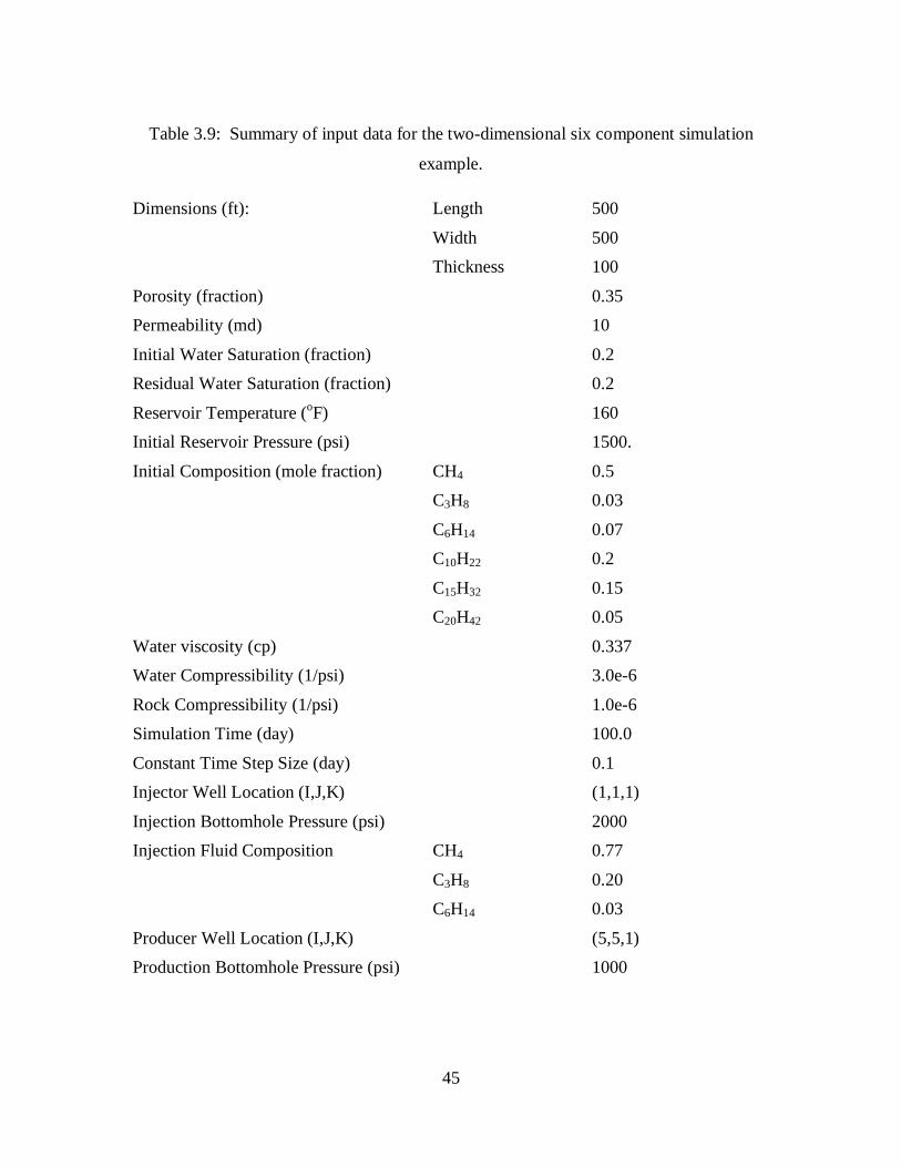
Table 3.9: Summary of input data for the two-dimensional six component simulation

example.

Dimensions (ft): Length 500

Width 500

Thickness 100

Porosity (fraction) 0.35

Permeability (md) 10

Initial Water Saturation (fraction) 0.2

Residual Water Saturation (fraction) 0.2

Reservoir Temperature (oF) 160

Initial Reservoir Pressure (psi) 1500.

Initial Composition (mole fraction) CH4 0.5

C3H8 0.03

C6H14 0.07

C10H22 0.2

C15H32 0.15

C20H42 0.05

Water viscosity (cp) 0.337

Water Compressibility (1/psi) 3.0e-6

Rock Compressibility (1/psi) 1.0e-6

Simulation Time (day) 100.0

Constant Time Step Size (day) 0.1

Injector Well Location (I,J,K) (1,1,1)

Injection Bottomhole Pressure (psi) 2000

Injection Fluid Composition CH4 0.77

C3H8 0.20

C6H14 0.03

Producer Well Location (I,J,K) (5,5,1)

Production Bottomhole Pressure (psi) 1000

46

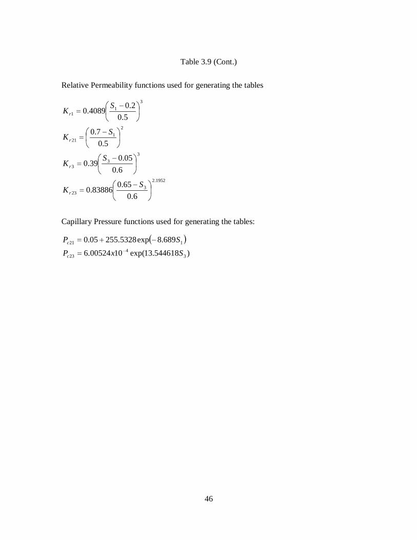
Table 3.9 (Cont.)


1952.23

23

33

3

21

21

31

1

6.065.0

83886.0

6.005.0

39.0

5.07.0

5.02.0

4089.0

��

��

� ��

��

��

� ��

��

��

� ��

��

��

� ��

SK

SK

SK

SK

r

r

r

r

Capillary Pressure functions used for generating the tables:

� �

)544618.13exp(1000524.6689.8exp5328.25505.0

34

23

121

SxPSP

c

c�

�

��

47

Table 3.10: Summary of input data for the three-dimensional six component simulation

example.


Porosity (fraction) 0.35Permeability (md) 10Initial Water Saturation (fraction) 0.2Residual Water Saturation (fraction) 0.2Reservoir Temperature (oF) 160Initial Reservoir Pressure (psi) 1500Initial Composition ( mole fraction) CH4 0.5

C3H8 0.03C6H14 0.07C10H22 0.2C15H32 0.15C20H42 0.05

Water viscosity (cp) 0.337Water Compressibility (1/psi) 3.0x10-5

Rock Compressibility (1/psi) 1.0e-6Simulation Time (day) 730.0Constant Time Step Size (day) 0.1Injector Well Top Location (I,J,K) (1,1,1)Injector Well Bottom Location (I,J,K) (1,1,5)Injection Bottomhole Pressure (psi) 1700Injection Fluid Composition CH4 0.77

C3H8 0.20C6H14 0.03

Producer Well Top Location (I,J,K) (10,10,1)Producer Well Bottom Location (I,J,K) (10,10,5)Production Bottomhole Pressure (psi) 1300

48

Table 3.10 (Cont.)

Relative Permeability functions used for generating the tables:

1952.23

23

33

3

21

21

31

1

6.065.0

83886.0

6.005.0

39.0

5.07.0

5.02.0

4089.0

��

��

� ��

��

��

� ��

��

��

� ��

��

��

� ��

SK

SK

SK

SK

r

r

r

r

Capillary Pressure functions used for generating the tables:

� �

)544618.13exp(1000524.6689.8exp5328.25505.0

34

23

121

SxPSP

c

c�

�

��

49

Frameworkof

IPARS

CompositionalModel

EOSCOMP

SolverPETSc

ChemicalModule

Figure 1.1: Flow chart showing the general structure of GPAS simulator

50

0.0

0.1

0.2

0.3

0.4

0.5

0.6

0.7

0.8

0.9

1.0

0.0 0.2 0.4 0.6 0.8 1.0Water Saturation, Sw

Phas

e Re

lativ

e Pe

rmea

bilit

y, k

rj

Oil Relative Permeability,kro

Water Relative Permeability,krw

Figure 3.1: Oil/Water relative permeability curves used in the Buckley Leverett

Problem.

0.00

0.20

0.40

0.60

0.80

1.00

0.00 0.20 0.40 0.60 0.80 1.00

Water Saturation, Sw

Frac

tiona

l Flo

w o

f Wat

er, f

w

Breakthrough

Figure 3.2: Fractional flow curve of water in the Buckley Leverett Problem.

51

Figu

re 3

.3:

Com

paris

on o

f th

e w

ater

sat

urat

ion

prof

ile f

rom

GPA

S w

ith t

he a

naly

tical

sol

utio

n a

nd t

he r

esul

t

from

UTC

HEM

at

0.1,

0.2

and

0.3

por

e vo

lum

es i

njec

ted

for

one-

dim

ensi

onal

Buc

kley

Lev

eret

t w

ater

flood

ing

52

Figu

re 3

.4:

Sche

mat

ic re

serv

oir g

eom

etry

(qua

rter f

ive

spot

) for

the

CO

2 seq

uest

ratio

n pr

oble

m.

53

1000

1100

1200

1300

1400

1500

1600

1700

1800

1900

2000

0 50 100 150 200 250 300 350 400 450 500

DISTANCE ALONG X AXIS, FT

PRES

SURE

, PSI

UTCOMP-LY1GPAS-LY1UTCOMP-LY2GPAS-LY2UTCOMP-LY3GPAS-LY3UTCOMP-LY4GPAS-LY4UTCOMP-LY5GPAS-LY5

LY = 1

LY = 2LY = 3

LY = 4

LY = 5

Figure 3.5: Comparison of the pressure profile along the x-axis obtained from

GPAS with UTCOMP at the end of 100 days for CO2 sequestration problem.

0.00

0.10

0.20

0.30

0.40

0.50

0.60

0.70

0 50 100 150 200 250 300 350 400 450 500DISTANCE ALONG X AXIS, FT

GASSATURATION,VOL/VOL


LY = 1

LY = 2

LY = 3

LY = 4

LY = 5

Figure 3.6: Comparison of the gas saturation profile along the x-axis from GPAS

with UTCOMP at the end of 100 days for the CO2 sequestration problem.

54

1000

1100

1200

1300

1400

1500

1600

1700

1800

1900

2000


PRES

SURE

, PSI


LY = 1

LY = 2LY = 3

LY = 4

LY = 5

Figure 3.7: Comparison of the pressure profile along the x-axis from GPAS with

UTCOMP at the end of 100 days for the six component problem.

0.00

0.10

0.20

0.30

0.40

0.50

0.60

0.70


OIL

SA

TUR

ATI

ON

,VO

L/VO

L


LY = 1LY = 2

LY = 3

LY = 4 LY = 5

Figure 3.8: Comparison of the oil saturation profile along the x-axis from GPAS

with UTCOMP at the end of 100 days for the six component problem.

55

0.00

0.05

0.10

0.15

0.20

0.25

0.30

0.35

0.40

0.45

0.50


GA

S SA

TUR

ATI

ON

,VO

L/VO

LUTCOMP-LY1GPAS-LY1UTCOMP-LY2GPAS-LY2UTCOMP-LY3GPAS-LY3UTCOMP-LY4GPAS-LY4UTCOMP-LY5GPAS-LY5

LY = 1LY = 2

LY = 3

LY = 4 LY = 5

Figure 3.9: Comparison of the gas saturation profile along the x axis from GPAS

with UTCOMP at the end of 100 days for the six component problem.

56

Figu

re 3

.10

Sch

emat

ic re

serv

oir g

eom

etry

for

the

thre

e di

men

sion

al si

x co

mpo

nent

sim

ulat

ion

case

.

57

1300

1350

1400

1450

1500

1550

1600

1650

1700


PRES

SURE

, PSI

UTCOMP-Ly2GPAS-Ly2UTCOMP-Ly4GPAS-Ly4UTCOMP-Ly6GPAS-Ly6UTCOMP-Ly8GPAS-Ly8UTCOMP-Ly10GPAS-Ly10

LY = 2LY = 4

LY = 6LY = 8

LY = 10

Figure 3.11: Comparison of the pressure profile along the x-axis from GPAS

with UTCOMP for the six component case at the end of two years.

0.00

0.05

0.10

0.15

0.20

0.25

0.30

0.35

0.40

0.45

0.50


OIL

SAT

URAT

ION

,VO

L/VO

L

UTCOMP-Ly1

GPAS-Ly1

UTCOMP-Ly10

GPAS-Ly10

LY = 1

LY = 10

Figure 3.12: Comparison of the oil saturation profile along the x-axis from GPAS

with UTCOMP for the six component case at the end of two years.

58

0.00

0.10

0.20

0.30

0.40

0.50

0.60

0.70

0.80


OIL

SAT

URAT

ION

,VO

L/VO

L

UTCOMP-Ly1

GPAS-Ly1

UTCOMP-Ly10

GPAS-Ly10

LY = 1LY = 10

Figure 3.13: Comparison of the gas saturation profile along the x-axis from

GPAS with UTCOMP for the six component case at the end of two years.

1.30E+03

1.35E+03

1.40E+03

1.45E+03

1.50E+03

1.55E+03

1.60E+03

1.65E+03

1.70E+03

0 100 200 300 400 500 600 700 800

Time, days

Aver

age

Rese

rvoi

r Pre

ssur

e, p

sia

GPAS

UTCOMP

Figure 3.14: Comparison of the average reservoir pressure history from GPAS

with UTCOMP for the six component case.

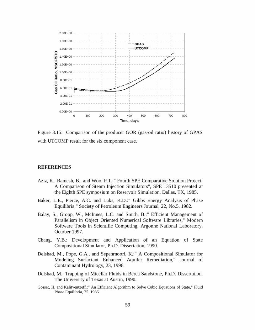
59

0.00E+00

2.00E-01

4.00E-01

6.00E-01

8.00E-01

1.00E+00

1.20E+00

1.40E+00

1.60E+00

1.80E+00

2.00E+00

0 100 200 300 400 500 600 700 800

Time, days

Gas

Oil

Rat

io, M

SCF/

STB

GPASUTCOMP

Figure 3.15: Comparison of the producer GOR (gas-oil ratio) history of GPAS

with UTCOMP result for the six component case.

REFERENCES

Aziz, K., Ramesh, B., and Woo, P.T.:" Fourth SPE Comparative Solution Project:A Comparison of Steam Injection Simulators", SPE 13510 presented atthe Eighth SPE symposium on Reservoir Simulation, Dallas, TX, 1985.

Baker, L.E., Pierce, A.C. and Luks, K.D.:" Gibbs Energy Analysis of PhaseEquilibria," Society of Petroleum Engineers Journal, 22, No.5, 1982.

Balay, S., Gropp, W., McInnes, L.C. and Smith, B.:" Efficient Management ofParallelism in Object Oriented Numerical Software Libraries," ModernSoftware Tools in Scientific Computing, Argonne National Laboratory,October 1997.

Chang, Y.B.: Development and Application of an Equation of StateCompositional Simulator, Ph.D. Dissertation, 1990.

Delshad, M., Pope, G.A., and Sepehrnoori, K.:" A Compositional Simulator forModeling Surfactant Enhanced Aquifer Remediation," Journal ofContaminant Hydrology, 23, 1996.

Delshad, M.: Trapping of Micellar Fluids in Berea Sandstone, Ph.D. Dissertation,The University of Texas at Austin, 1990.

Gosset, H. and Kalitventzeff.:" An Efficient Algorithm to Solve Cubic Equations of State," FluidPhase Equilibria, 25 ,1986.

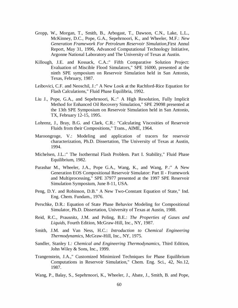
60

Gropp, W., Morgan, T., Smith, B., Arbogast, T., Dawson, C.N., Lake, L.L.,McKinney, D.C., Pope, G.A., Sepehrnoori, K., and Wheeler, M.F.: NewGeneration Framework For Petroleum Reservoir Simulation,First AnnulReport, May 31, 1996, Advanced Computational Technology Initiative,Argonne National Laboratory and The University of Texas at Austin.

Killough, J.E. and Kossack, C.A.:" Fifth Comparative Solution Project:Evaluation of Miscible Flood Simulators," SPE 16000, presented at theninth SPE symposium on Reservoir Simulation held in San Antonio,Texas, February, 1987.

Leibovici, C.F. and Neoschil, J.:" A New Look at the Rachford-Rice Equation forFlash Calculations," Fluid Phase Equilibria, 1992.

Liu J., Pope, G.A., and Sepehrnoori, K.:" A High Resolution, Fully ImplicitMethod for Enhanced Oil Recovery Simulation," SPE 29098 presented atthe 13th SPE Symposium on Reservoir Simulation held in San Antonio,TX, February 12-15, 1995.

Lohrenz, J., Bray, B.G. and Clark, C.R.: "Calculating Viscosities of ReservoirFluids from their Compositions," Trans., AIME, 1964.

Maroongroge, V.: Modeling and application of tracers for reservoircharacterization, Ph.D. Dissertation, The University of Texas at Austin,1994.

Michelsen, J.L.:" The Isothermal Flash Problem. Part I. Stability," Fluid PhaseEquilibrium, 1982.

Parashar M., Wheeler, J.A., Pope G.A., Wang, K., and Wang, P.:" A NewGeneration EOS Compositional Reservoir Simulator: Part II - Frameworkand Multiprocessing," SPE 37977 presented at the 1997 SPE ReservoirSimulation Symposium, June 8-11, USA.

Peng, D.Y. and Robinson, D.B." A New Two-Constant Equation of State," Ind.Eng. Chem. Fundam., 1976.

Perschke, D.R.: Equation of State Phase Behavior Modeling for CompositionalSimulator, Ph.D. Dissertation, University of Texas at Austin, 1988.

Reid, R.C., Prausnitz, J.M. and Poling, B.E.: The Properties of Gases andLiquids, Fourth Edition, McGraw-Hill, Inc., NY, 1987.

Smith, J.M. and Van Ness, H.C.: Introduction to Chemical EngineeringThermodynamics, McGraw-Hill, Inc., NY, 1975.

Sandler, Stanley I.: Chemical and Engineering Thermodynamics, Third Edition,John Wiley & Sons, Inc., 1999.

Trangenstein, J.A.," Customized Minimized Techniques for Phase EquilibriumComputations in Reservoir Simulation," Chem. Eng. Sci., 42, No.12,1987.

Wang, P., Balay, S., Sepehrnoori, K., Wheeler, J., Abate, J., Smith, B. and Pope,

61

G.A.:" A Fully Implicit Parallel EOS.Compositional Simulator for LargeScale Reservoir Simulation," SPE 51885 presented at the 1999 SPE 15th

Reservoir Simulation Symposium, Houston, TX, Feb. 14-17, 1999.

Wang, P., Yotov, I., Wheeler, M., Arbogast, T., Dawson, C., Parashar, M. andSepehrnoori, K.:" A New Generation EOS Compositional ReservoirSimulator: Part I - Formulation and Discretization," SPE 37979 presentedat the 1997 SPE Reservoir Simulation Symposium, USA.

Wheeler, J., et al.: IPARS user's manual, October 8,2000, University of Texas atAustin.

Documents

Semi-Annual Report, Feb. 2002