Semantics of Programming Languages -

Autumn 2004

Matthew Hennessy

Course Notes by Guy McCusker

Note: Not all the topics in these notes will be coveredin Autumn 2007 course

1 Introduction

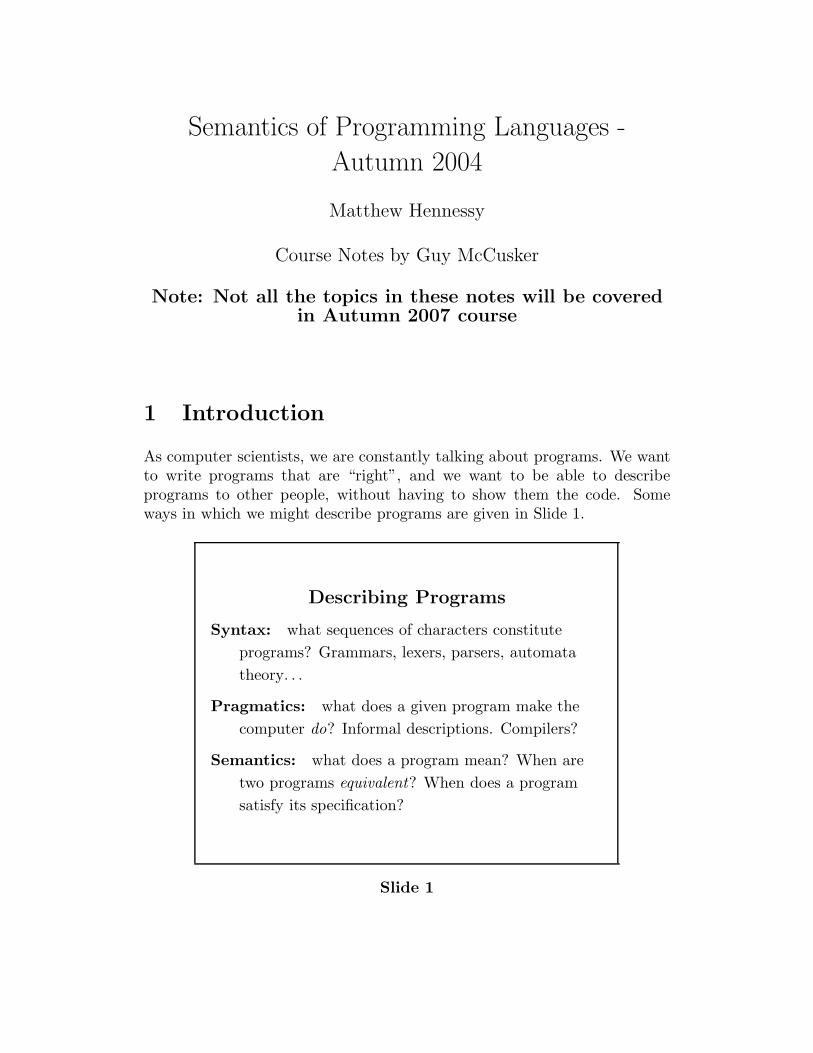
As computer scientists, we are constantly talking about programs. We wantto write programs that are “right”, and we want to be able to describeprograms to other people, without having to show them the code. Someways in which we might describe programs are given in Slide 1.

Describing Programs

Syntax: what sequences of characters constitute

programs? Grammars, lexers, parsers, automata

theory. . .

Pragmatics: what does a given program make the

computer do? Informal descriptions. Compilers?

Semantics: what does a program mean? When are

two programs equivalent? When does a program

satisfy its specification?

Slide 1

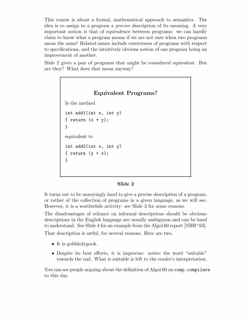
This course is about a formal, mathematical approach to semantics. Theidea is to assign to a program a precise description of its meaning. A veryimportant notion is that of equivalence between programs: we can hardlyclaim to know what a program means if we are not sure when two programsmean the same! Related issues include correctness of programs with respectto specifications, and the intuitively obvious notion of one program being animprovement of another.

Slide 2 gives a pair of programs that might be considered equivalent. Butare they? What does that mean anyway?

Equivalent Programs?

Is the method

int add1(int x, int y)

{ return (x + y);

}

equivalent to

int add2(int x, int y)

{ return (y + x);

}

Slide 2

It turns out to be annoyingly hard to give a precise description of a program,or rather of the collection of programs in a given language, as we will see.However, it is a worthwhile activity: see Slide 3 for some reasons.

The disadvantages of reliance on informal descriptions should be obvious:descriptions in the English language are usually ambiguous and can be hardto understand. See Slide 4 for an example from the Algol 60 report [NBB+63].

That description is awful, for several reasons. Here are two.

• It is gobbledygook.

• Despite its best efforts, it is imprecise: notice the word “suitable”towards the end. What is suitable is left to the reader’s interpretation.

You can see people arguing about the definition of Algol 60 on comp.compilersto this day.

Benefits of Formal Semantics

Implementation: correctness of compilers, including

optimisations, static analyses etc.

Verification: semantics supports reasoning about

programs, specifications and other properties, both

mechanically and by hand.

Language design: subtle ambiguities in existing

languages often come to light, and cleaner, clearer

ways of organising things can be discovered.

Slide 3

Informal Descriptions

An extract from the Algol 60 report:

Finally the procedure body, modified as above, is

inserted in place of the procedure statement and

executed. If a procedure is called from a place

outside the scope of any nonlocal quantity of the

procedure body, the conflicts between the identifiers

inserted through this process of body replacement

and the identifiers whose declarations are valid at

the place of the procedure statement or function

designator will be avoided through suitable

systematic changes of the latter identifiers.

Slide 4

1.1 Styles of Semantics

There are several different, complementary styles of formal semantics. Threeof the most important are denotational, operational and axiomatic semantics.We shall have at least a quick look at each of these styles.

Styles of Semantics

Denotational: a program’s meaning is given

abstractly as an element of some mathematical

structure (some kind of set).

Operational: a program’s meaning is given in terms

of the steps of computation the program makes

when you run it.

Axiomatic: a program’s meaning is given indirectly

in terms of the collection of properties it satisfies;

these properties are defined via a collection of

axioms and rules.

Slide 5

The effort to make semantics precise has been underway since the late 1960s,and many deep and interesting discoveries have been made. However, we area very long way from having a complete, usable theory of programminglanguage semantics which accommodates the prevalent features of modernlanguages. So be warned: the languages we consider on this course will bevery simplistic.

2 A Language of Expressions

Let us begin by considering a very simple language of arithmetic expressions.This example will serve to illustrate some of the ideas behind the variouskinds of semantics, and will provide a simple setting in which to introduceinductive definitions and proofs slightly later on.

A grammar for a simple language Exp of expressions is given on Slide 9.

We all know what these things mean intuitively, and we expect that, forexample, (3 + 7) and (5× 2) mean the same thing.

The state of the art

Denotational: successful research has focused on

very simple imperative languages and vastly

complex but seldom-used functional languages.

Operational: most sequential languages and some

concurrent languages can be given operational

semantics, but the theory tends to be hard to use.

Axiomatic: beyond simple imperative languages,

little has been done.

Slide 6

This course: semantics

We will consider:

• operational, axiomatic and denotational semantics

for a very simple imperative language;

• ways of proving facts about the semantics; and

• connections between the various semantics.

Slide 7

This course: maths

There will be some mathematics along the way:

• mathematical induction; and

• structural induction.

Slide 8

Syntax of Exp

E ∈ Exp ::= n | (E + E) | (E × E) | · · ·

where n ranges over the numerals 0, 1, . . . . We can add

more operations if we need to.

We will always work with abstract syntax. That is, we

assume all programs have already been parsed, so the

grammar above defines syntax trees rather than

concrete syntax.

Slide 9

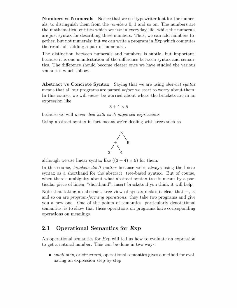
Numbers vs Numerals Notice that we use typewriter font for the numer-als, to distinguish them from the numbers 0, 1 and so on. The numbers arethe mathematical entities which we use in everyday life, while the numeralsare just syntax for describing these numbers. Thus, we can add numbers to-gether, but not numerals; but we can write a program in Exp which computesthe result of “adding a pair of numerals”.

The distinction between numerals and numbers is subtle, but important,because it is one manifestation of the difference between syntax and seman-tics. The difference should become clearer once we have studied the varioussemantics which follow.

Abstract vs Concrete Syntax Saying that we are using abstract syntaxmeans that all our programs are parsed before we start to worry about them.In this course, we will never be worried about where the brackets are in anexpression like

3 + 4× 5

because we will never deal with such unparsed expressions.

Using abstract syntax in fact means we’re dealing with trees such as

×

+

3 4

5

although we use linear syntax like ((3 + 4) × 5) for them.

In this course, brackets don’t matter because we’re always using the linearsyntax as a shorthand for the abstract, tree-based syntax. But of course,when there’s ambiguity about what abstract syntax tree is meant by a par-ticular piece of linear “shorthand”, insert brackets if you think it will help.

Note that taking an abstract, tree-view of syntax makes it clear that +, ×and so on are program-forming operations: they take two programs and giveyou a new one. One of the points of semantics, particularly denotationalsemantics, is to show that these operations on programs have correspondingoperations on meanings.

2.1 Operational Semantics for Exp

An operational semantics for Exp will tell us how to evaluate an expressionto get a natural number. This can be done in two ways:

• small-step, or structural, operational semantics gives a method for eval-uating an expression step-by-step

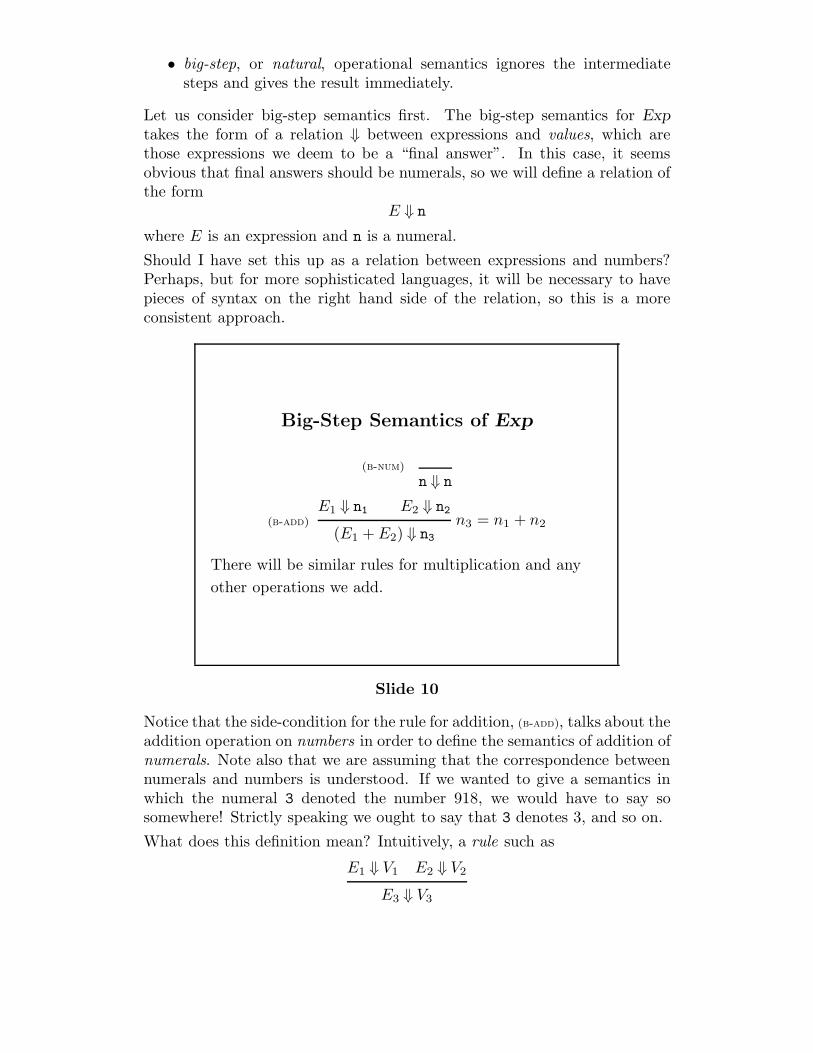
• big-step, or natural, operational semantics ignores the intermediatesteps and gives the result immediately.

Let us consider big-step semantics first. The big-step semantics for Exp

takes the form of a relation ⇓ between expressions and values, which arethose expressions we deem to be a “final answer”. In this case, it seemsobvious that final answers should be numerals, so we will define a relation ofthe form

E ⇓ n

where E is an expression and n is a numeral.

Should I have set this up as a relation between expressions and numbers?Perhaps, but for more sophisticated languages, it will be necessary to havepieces of syntax on the right hand side of the relation, so this is a moreconsistent approach.

Big-Step Semantics of Exp

(b-num)

n ⇓ n

(b-add)E1 ⇓ n1 E2 ⇓ n2

n3 = n1 + n2(E1 + E2) ⇓ n3

There will be similar rules for multiplication and any

other operations we add.

Slide 10

Notice that the side-condition for the rule for addition, (b-add), talks about theaddition operation on numbers in order to define the semantics of addition ofnumerals. Note also that we are assuming that the correspondence betweennumerals and numbers is understood. If we wanted to give a semantics inwhich the numeral 3 denoted the number 918, we would have to say sosomewhere! Strictly speaking we ought to say that 3 denotes 3, and so on.

What does this definition mean? Intuitively, a rule such as

E1 ⇓ V1 E2 ⇓ V2

E3 ⇓ V3

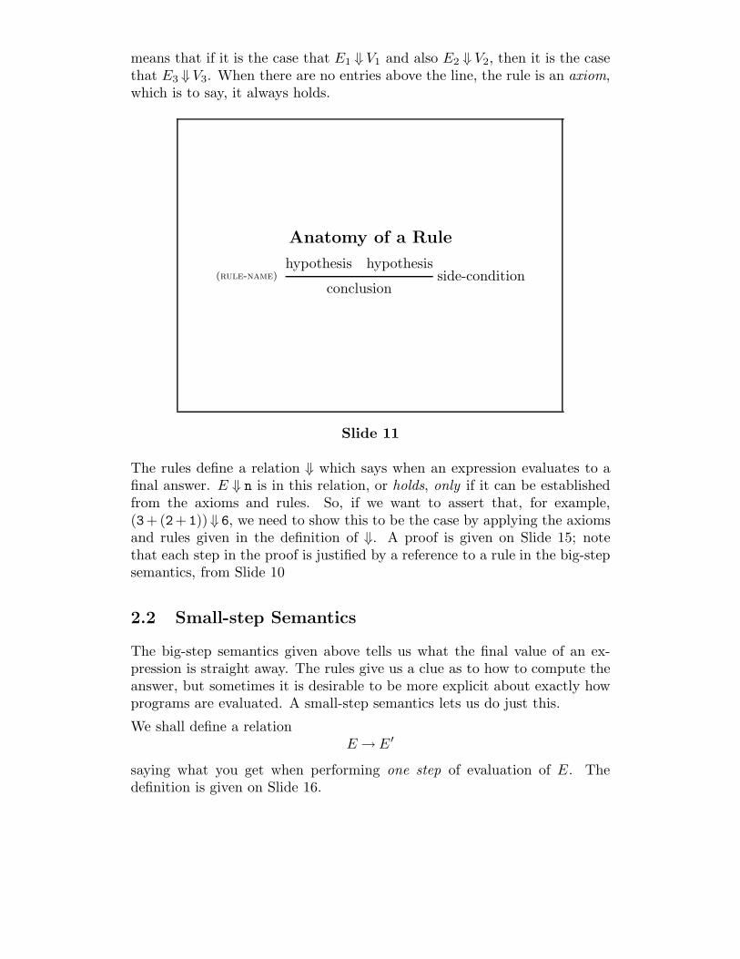
means that if it is the case that E1 ⇓ V1 and also E2 ⇓ V2, then it is the casethat E3 ⇓V3. When there are no entries above the line, the rule is an axiom,which is to say, it always holds.

Anatomy of a Rule

(rule-name)hypothesis hypothesis

side-conditionconclusion

Slide 11

The rules define a relation ⇓ which says when an expression evaluates to afinal answer. E ⇓ n is in this relation, or holds, only if it can be establishedfrom the axioms and rules. So, if we want to assert that, for example,(3+(2+1))⇓ 6, we need to show this to be the case by applying the axiomsand rules given in the definition of ⇓. A proof is given on Slide 15; notethat each step in the proof is justified by a reference to a rule in the big-stepsemantics, from Slide 10

2.2 Small-step Semantics

The big-step semantics given above tells us what the final value of an ex-pression is straight away. The rules give us a clue as to how to compute theanswer, but sometimes it is desirable to be more explicit about exactly howprograms are evaluated. A small-step semantics lets us do just this.

We shall define a relationE → E′

saying what you get when performing one step of evaluation of E. Thedefinition is given on Slide 16.

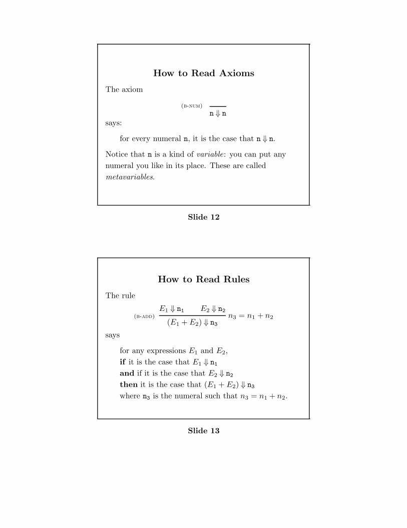
How to Read Axioms

The axiom

(b-num)

n ⇓ nsays:

for every numeral n, it is the case that n ⇓ n.

Notice that n is a kind of variable: you can put any

numeral you like in its place. These are called

metavariables.

Slide 12

How to Read Rules

The rule

(b-add)E1 ⇓ n1 E2 ⇓ n2

n3 = n1 + n2(E1 + E2) ⇓ n3

says

for any expressions E1 and E2,

if it is the case that E1 ⇓ n1

and if it is the case that E2 ⇓ n2

then it is the case that (E1 + E2) ⇓ n3

where n3 is the numeral such that n3 = n1 + n2.

Slide 13

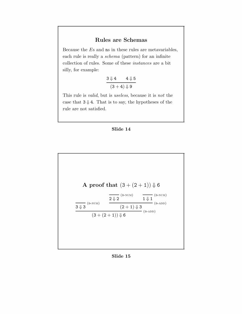
Rules are Schemas

Because the Es and ns in these rules are metavariables,

each rule is really a schema (pattern) for an infinite

collection of rules. Some of these instances are a bit

silly, for example:

3 ⇓ 4 4 ⇓ 5

(3 + 4) ⇓ 9

This rule is valid, but is useless, because it is not the

case that 3 ⇓ 4. That is to say, the hypotheses of the

rule are not satisfied.

Slide 14

A proof that (3 + (2 + 1)) ⇓ 6

(b-num)3 ⇓ 3

(b-num)2 ⇓ 2

(b-num)1 ⇓ 1

(b-add)(2 + 1) ⇓ 3

(b-add)(3 + (2 + 1)) ⇓ 6

Slide 15

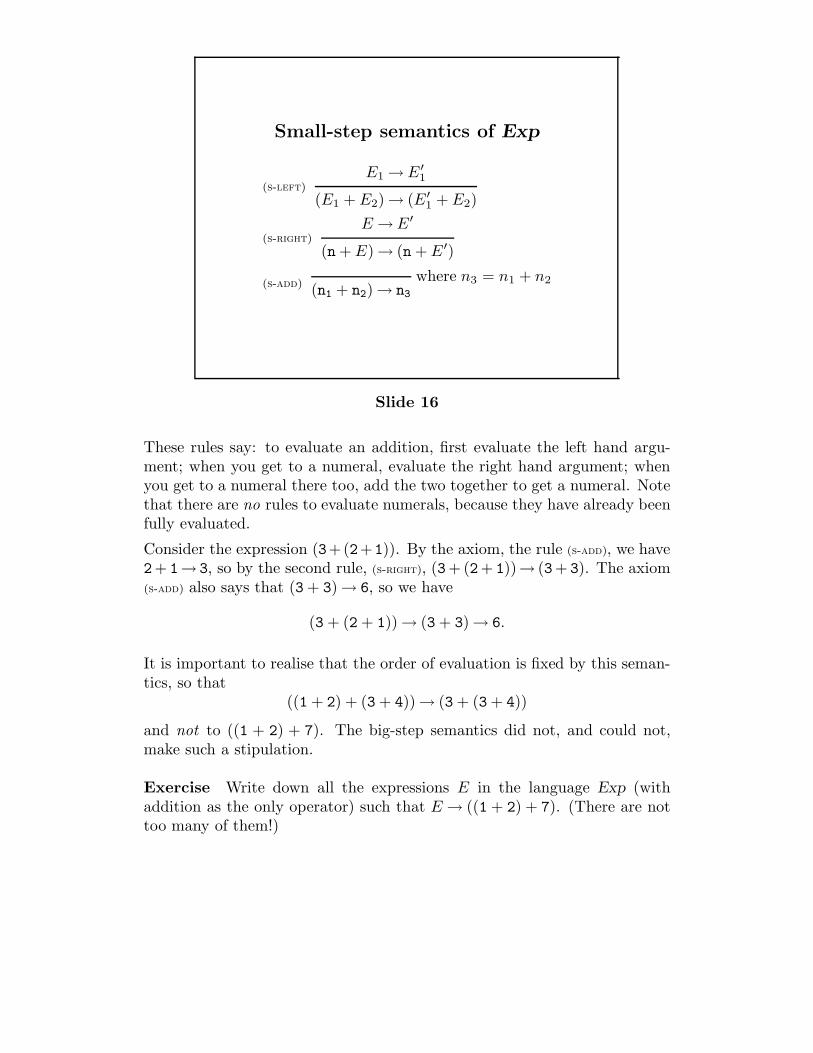
Small-step semantics of Exp

(s-left)E1 → E′

1

(E1 + E2) → (E′

1 + E2)

(s-right)E → E′

(n + E) → (n + E′)

(s-add)where n3 = n1 + n2

(n1 + n2) → n3

Slide 16

These rules say: to evaluate an addition, first evaluate the left hand argu-ment; when you get to a numeral, evaluate the right hand argument; whenyou get to a numeral there too, add the two together to get a numeral. Notethat there are no rules to evaluate numerals, because they have already beenfully evaluated.

Consider the expression (3+(2+1)). By the axiom, the rule (s-add), we have2+ 1→ 3, so by the second rule, (s-right), (3+(2+ 1))→ (3+ 3). The axiom(s-add) also says that (3 + 3) → 6, so we have

(3 + (2 + 1)) → (3 + 3) → 6.

It is important to realise that the order of evaluation is fixed by this seman-tics, so that

((1 + 2) + (3 + 4)) → (3 + (3 + 4))

and not to ((1 + 2) + 7). The big-step semantics did not, and could not,make such a stipulation.

Exercise Write down all the expressions E in the language Exp (withaddition as the only operator) such that E → ((1 + 2) + 7). (There are nottoo many of them!)

2.2.1 Getting the final answer

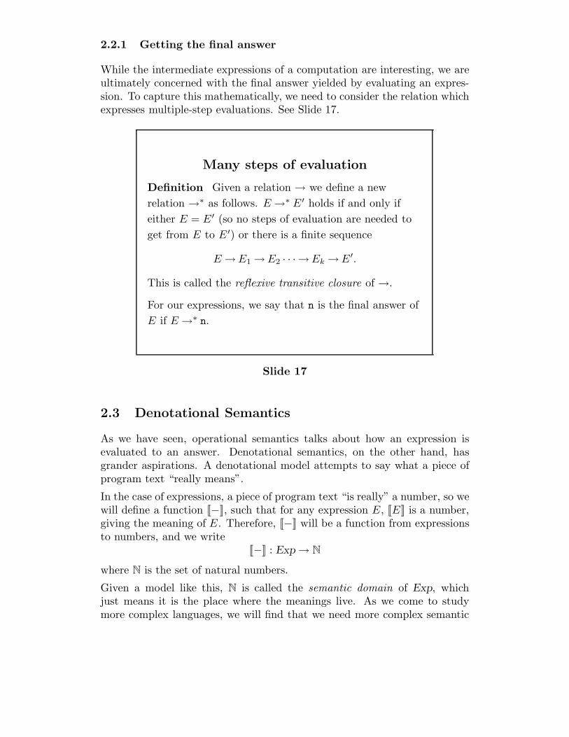
While the intermediate expressions of a computation are interesting, we areultimately concerned with the final answer yielded by evaluating an expres-sion. To capture this mathematically, we need to consider the relation whichexpresses multiple-step evaluations. See Slide 17.

Many steps of evaluation

Definition Given a relation → we define a new

relation →∗ as follows. E →∗ E′ holds if and only if

either E = E′ (so no steps of evaluation are needed to

get from E to E′) or there is a finite sequence

E → E1 → E2 · · ·→ Ek → E′.

This is called the reflexive transitive closure of →.

For our expressions, we say that n is the final answer of

E if E →∗ n.

Slide 17

2.3 Denotational Semantics

As we have seen, operational semantics talks about how an expression isevaluated to an answer. Denotational semantics, on the other hand, hasgrander aspirations. A denotational model attempts to say what a piece ofprogram text “really means”.

In the case of expressions, a piece of program text “is really” a number, so wewill define a function [[−]], such that for any expression E, [[E]] is a number,giving the meaning of E. Therefore, [[−]] will be a function from expressionsto numbers, and we write

[[−]] : Exp → N

where N is the set of natural numbers.

Given a model like this, N is called the semantic domain of Exp, whichjust means it is the place where the meanings live. As we come to studymore complex languages, we will find that we need more complex semantic

Denotational semantics

We will define the denotational semantics of expressions

via a function

[[−]] : Exp → N.

Slide 18

domains. The construction and study of such domains is the subject ofdomain theory, an elegant mathematical theory which provides a foundationfor denotational semantics; unfortunately domain theory is beyond the scopeof this course.

For now, notice that our choice of semantic domain has certain consequencesfor the semantics of our language: it implies that every expression will“mean” exactly one number, so without even seeing the definition of [[−]],someone looking at our semantics already knows that the language is (ex-pected to be) normalising (every expression has an answer) and deterministic(each expression has at most one answer).

It is easy to give a meaning to numerals:

[[n]] = n.

Note again the difference between numerals and numbers, or syntax andsemantics.

For addition expressions (E1 + E2), the meaning will of course be the sumof the meanings of E1 and E2:

[[(E1 + E2)]] = [[E1]] + [[E2]].

We could make similar definitions for multiplication and so on.

We have defined [[−]] by induction on the structure of expressions: see Sec-tion 3.

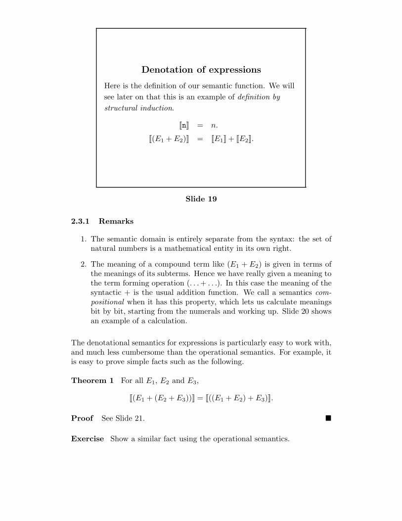
Denotation of expressions

Here is the definition of our semantic function. We will

see later on that this is an example of definition by

structural induction.

[[n]] = n.

[[(E1 + E2)]] = [[E1]] + [[E2]].

Slide 19

2.3.1 Remarks

1. The semantic domain is entirely separate from the syntax: the set ofnatural numbers is a mathematical entity in its own right.

2. The meaning of a compound term like (E1 + E2) is given in terms ofthe meanings of its subterms. Hence we have really given a meaning tothe term forming operation (. . .+ . . .). In this case the meaning of thesyntactic + is the usual addition function. We call a semantics com-positional when it has this property, which lets us calculate meaningsbit by bit, starting from the numerals and working up. Slide 20 showsan example of a calculation.

The denotational semantics for expressions is particularly easy to work with,and much less cumbersome than the operational semantics. For example, itis easy to prove simple facts such as the following.

Theorem 1 For all E1, E2 and E3,

[[(E1 + (E2 + E3))]] = [[((E1 + E2) + E3)]].

Proof See Slide 21. !

Exercise Show a similar fact using the operational semantics.

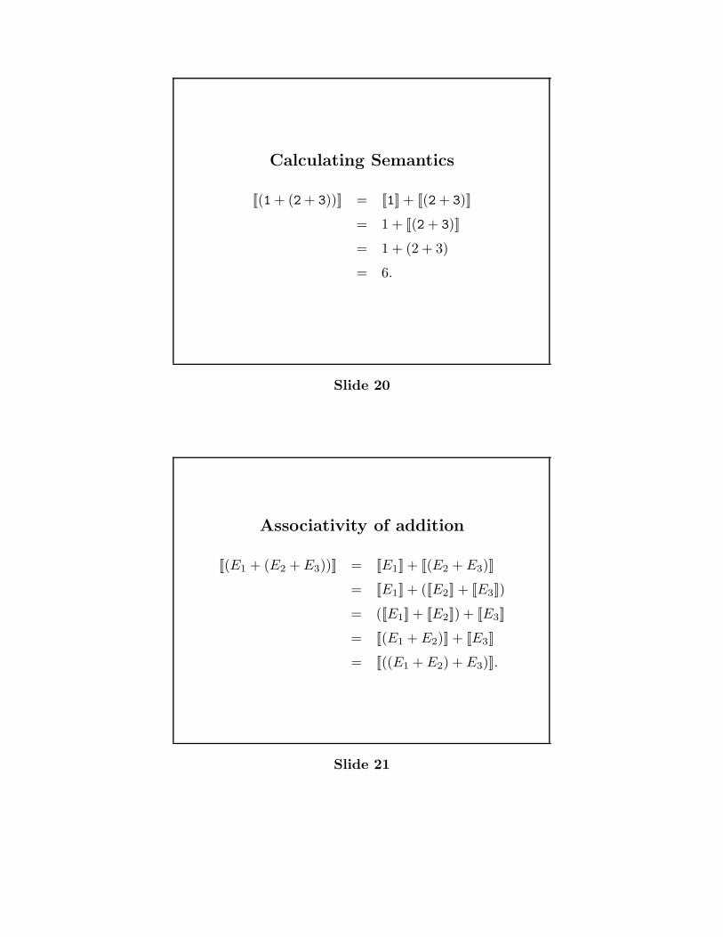
Calculating Semantics

[[(1 + (2 + 3))]] = [[1]] + [[(2 + 3)]]

= 1 + [[(2 + 3)]]

= 1 + (2 + 3)

= 6.

Slide 20

Associativity of addition

[[(E1 + (E2 + E3))]] = [[E1]] + [[(E2 + E3)]]

= [[E1]] + ([[E2]] + [[E3]])

= ([[E1]] + [[E2]]) + [[E3]]

= [[(E1 + E2)]] + [[E3]]

= [[((E1 + E2) + E3)]].

Slide 21

2.4 Contextual Equivalence

We shall now introduce a very important idea in semantics, that of contextualequivalence.

One thing we might expect of equivalent programs is that they can be usedinterchangeably. That is, if P1

∼= P2 and P1 is used in some context, C[P1],then we should get the same effect if we replace P1 with P2: we expectC[P1] ∼= C[P2].

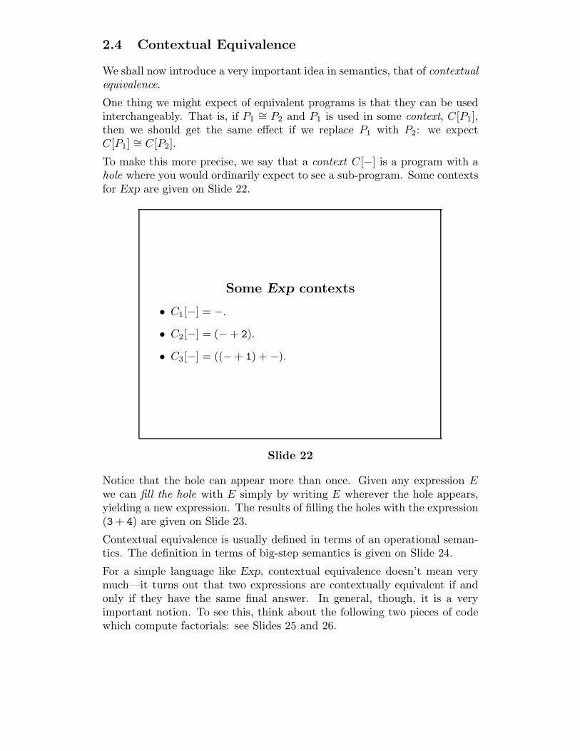
To make this more precise, we say that a context C[−] is a program with ahole where you would ordinarily expect to see a sub-program. Some contextsfor Exp are given on Slide 22.

Some Exp contexts

• C1[−] = −.

• C2[−] = (− + 2).

• C3[−] = ((− + 1) + −).

Slide 22

Notice that the hole can appear more than once. Given any expression Ewe can fill the hole with E simply by writing E wherever the hole appears,yielding a new expression. The results of filling the holes with the expression(3 + 4) are given on Slide 23.

Contextual equivalence is usually defined in terms of an operational seman-tics. The definition in terms of big-step semantics is given on Slide 24.

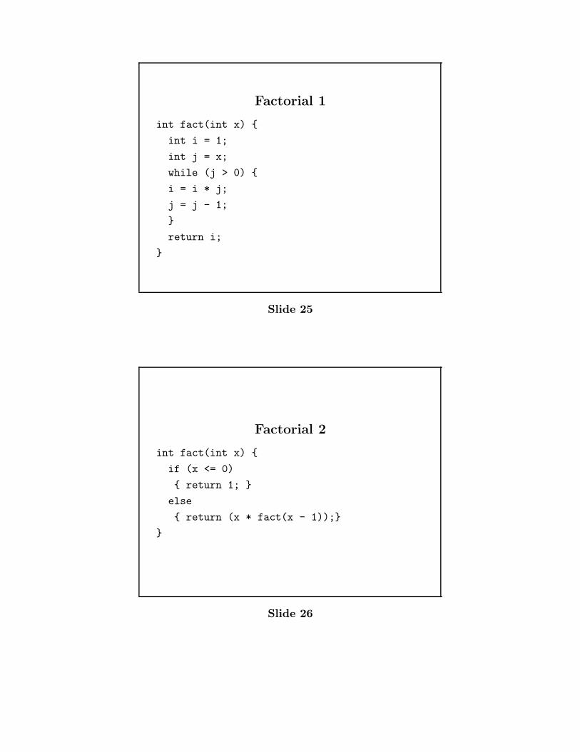
For a simple language like Exp, contextual equivalence doesn’t mean verymuch—it turns out that two expressions are contextually equivalent if andonly if they have the same final answer. In general, though, it is a veryimportant notion. To see this, think about the following two pieces of codewhich compute factorials: see Slides 25 and 26.

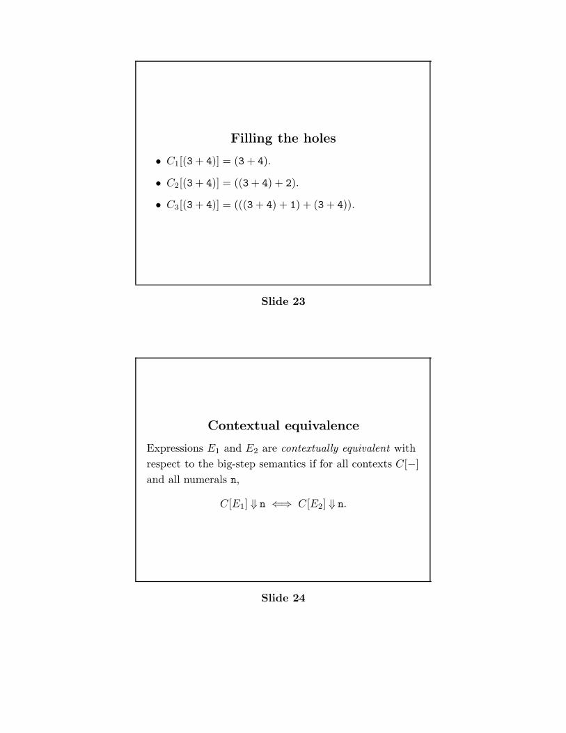
Filling the holes

• C1[(3 + 4)] = (3 + 4).

• C2[(3 + 4)] = ((3 + 4) + 2).

• C3[(3 + 4)] = (((3 + 4) + 1) + (3 + 4)).

Slide 23

Contextual equivalence

Expressions E1 and E2 are contextually equivalent with

respect to the big-step semantics if for all contexts C[−]

and all numerals n,

C[E1] ⇓ n ⇐⇒ C[E2] ⇓ n.

Slide 24

Factorial 1

int fact(int x) {

int i = 1;

int j = x;

while (j > 0) {

i = i * j;

j = j - 1;

}

return i;

}

Slide 25

Factorial 2

int fact(int x) {

if (x <= 0)

{ return 1; }

else

{ return (x * fact(x - 1));}

}

Slide 26

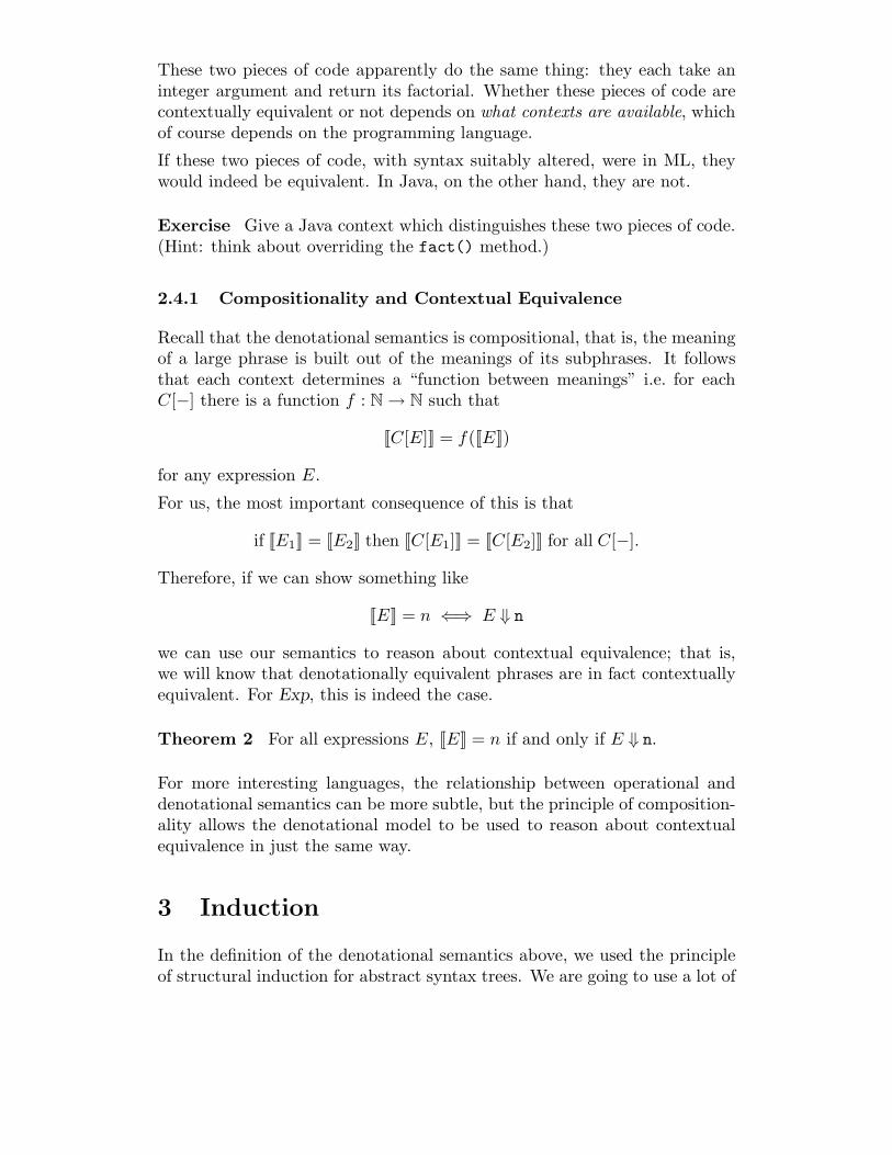
These two pieces of code apparently do the same thing: they each take aninteger argument and return its factorial. Whether these pieces of code arecontextually equivalent or not depends on what contexts are available, whichof course depends on the programming language.

If these two pieces of code, with syntax suitably altered, were in ML, theywould indeed be equivalent. In Java, on the other hand, they are not.

Exercise Give a Java context which distinguishes these two pieces of code.(Hint: think about overriding the fact() method.)

2.4.1 Compositionality and Contextual Equivalence

Recall that the denotational semantics is compositional, that is, the meaningof a large phrase is built out of the meanings of its subphrases. It followsthat each context determines a “function between meanings” i.e. for eachC[−] there is a function f : N → N such that

[[C[E]]] = f([[E]])

for any expression E.

For us, the most important consequence of this is that

if [[E1]] = [[E2]] then [[C[E1]]] = [[C[E2]]] for all C[−].

Therefore, if we can show something like

[[E]] = n ⇐⇒ E ⇓ n

we can use our semantics to reason about contextual equivalence; that is,we will know that denotationally equivalent phrases are in fact contextuallyequivalent. For Exp, this is indeed the case.

Theorem 2 For all expressions E, [[E]] = n if and only if E ⇓ n.

For more interesting languages, the relationship between operational anddenotational semantics can be more subtle, but the principle of composition-ality allows the denotational model to be used to reason about contextualequivalence in just the same way.

3 Induction

In the definition of the denotational semantics above, we used the principleof structural induction for abstract syntax trees. We are going to use a lot of

Our first correspondence theorem

For all expressions E, [[E]] = n if and only if

E ⇓ n.

Slide 27

inductive techniques in this course, both to give definitions and to prove factsabout our semantics. So, it’s worth taking a little while to set out exactlywhat a proof by induction is, what a definition by induction is, and so on.

Very often in computer science, and (less often) in life in general, we comeup against the problem of reasoning about unknown entities. For example,when designing an algorithm to solve a problem, we want to know that theresult produced by the algorithm is correct, regardless of the input:

The quicksort algorithm takes a list of numbers and puts theminto ascending order.

In this example, we know that the algorithm operates on a list of numbers,but we do not know how long that list is or exactly what numbers it contains.Similarly one may raise questions about depth-first search of a tree: how dowe know it always visits all the nodes of a tree if we do not know the exactsize and shape of the tree?

In examples such as these, there are two important facts about the inputdata which allow us to reason about arbitrary inputs:

• the input is structured in a known way; for example, a non-empty listhas a first element and a “tail”, which is the rest of the list, and abinary tree has a root node and two subtrees.

• the input is finite.

In this situation, the technique of structural induction provides a principleby which we may formally reason about arbitrary lists, trees and so on.

What’s induction for?

Induction is a technique for reasoning about and

working with collections of objects (things!) which are

• structured in some well-defined way,

• finite but arbitrarily large and complex.

Induction exploits the finite, structured nature of these

objects to overcome the arbitrary complexity.

Slide 28

These kinds of structured, finite objects arise in many areas of computer sci-ence. Data structures as above are a common example, but in fact programsthemselves can be seen as structured finite objects. This means that induc-tion can be used to prove facts about all programs in a certain language. Insemantics, we use this very frequently. We will also make use of inductionto reason about purely semantic notions, such as derivations of assertions inthe operational semantics of a language.

3.1 Mathematical Induction

The simplest form of induction is mathematical induction, that is to say, in-duction over the natural numbers. The principle can be described as follows.

Given a property P (−) of natural numbers, to prove that P (n) holds for allnatural numbers n, it is enough to

• prove that P (0) holds, and

• prove that if P (k) holds for an arbitrary natural number k,then P (k + 1) holds too.

It should be clear why this principle is valid: if we can prove the two thingsabove, then we know

You can use induction. . .

. . . to reason about things like

• natural numbers: each one is finite, but natural

numbers could be arbitrarily big

• data structures such as trees, lists and so on

• programs in a programming language: again, you

can write arbitrarily large programs, but they are

always finite

• derivations of semantic assertions like E ⇓ 4: these

derivations are finite trees of axioms and rules.

Slide 29

Proof by Mathematical Induction

Let P (−) be a property of natural numbers. The

principle of mathematical induction states that if

P (0) ∧ [∀k.P (k) =⇒ P (k + 1)]

holds then

∀n.P (n)

holds.

k is the induction parameter

Slide 30

Writing an inductive proof

To prove that P (n) holds for all natural numbers n, we

must do two things.

Base Case: prove that P (0) holds, any way you like

Inductive Step: let k be an arbitrary number, and

assume that P (k) holds. This assumption is called

the inductive hypothesis or IH, with parameter k.

Using this assumption, prove that P (k + 1) holds.

Slide 31

• P (0) holds.

• Since P (0) holds, P (1) holds.

• Since P (1) holds, P (2) holds.

• Since P (2) holds, P (3) holds.

• And so on. . .

Therefore, P (n) holds for any n, regardless of how big n is.

This conclusion can only be drawn because every natural number can bereached by starting at zero and adding one repeatedly. The two elements ofthe induction can be read as saying

• Prove that P is true at the place where you start, i.e. zero.

• Prove that the operation of adding one preserves P , that is, if P (k) istrue then P (k + 1) is true.

Since every natural number can be “built” by starting at zero and addingone repeatedly, every natural number has the property P : as you build thenumber, P is true of everything you build along the way, and it’s still truewhen you’ve built the number you’re really interested in.

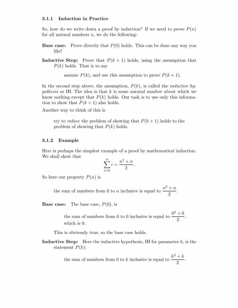
3.1.1 Induction in Practice

So, how do we write down a proof by induction? If we need to prove P (n)for all natural numbers n, we do the following:

Base case: Prove directly that P (0) holds. This can be done any way youlike!

Inductive Step: Prove that P (k + 1) holds, using the assumption thatP (k) holds. That is to say

assume P (k), and use this assumption to prove P (k + 1).

In the second step above, the assumption, P (k), is called the inductive hy-pothesis or IH. The idea is that k is some natural number about which weknow nothing except that P (k) holds. Our task is to use only this informa-tion to show that P (k + 1) also holds.

Another way to think of this is

try to reduce the problem of showing that P (k + 1) holds to theproblem of showing that P (k) holds.

3.1.2 Example

Here is perhaps the simplest example of a proof by mathematical induction.We shall show that

n∑

i=0

i =n2 + n

2.

So here our property P (n) is

the sum of numbers from 0 to n inclusive is equal ton2 + n

2.

Base case: The base case, P (0), is

the sum of numbers from 0 to 0 inclusive is equal to02 + 0

2,

which is 0.

This is obviously true, so the base case holds.

Inductive Step: Here the inductive hypothesis, IH for parameter k, is thestatement P (k):

the sum of numbers from 0 to k inclusive is equal tok2 + k

2.

From this inductive hypothesis, with parameter k, we must prove that

the sum of numbers from 0 to k + 1 inclusive is equal to(k + 1)2 + (k + 1)

2.

The proof is a simple calculation.

k+1∑

i=0

i = (k

∑

i=0

i) + (k + 1)

=k2 + k

2+ (k + 1) using IH for k

=k2 + k + 2k + 2

2

=(k2 + 2k + 1) + (k + 1)

2

=(k + 1)2 + (k + 1)

2

which is what we had to prove.

3.1.3 Defining Functions and Relations

As well as using induction to prove properties of natural numbers, we canuse it to define functions which operate on natural numbers.

Just as proof by induction proves a property P (n) by considering the case ofzero and the case of adding one to a number known to satisfy P , so definitionof a function f by induction works by giving the definition of f(0) directly,and building the value of f(k + 1) out of f(k).

All this is saying is that if you define the value of a function at zero, by givingsome a, and you show how to calculate the value at k + 1 from that at k,then this does indeed define a function. This function is “unique”, meaningthat it is completely defined by the information you have given—there is nochoice about what f can be.

Roughly, the fact that we use f(k) to define f(k + 1) in this definition cor-responds to the fact that we assume P (k) to prove P (k + 1) in a proof byinduction.

For example, Slide 33 gives an inductive definition of the factorial functionover the natural numbers.

Slide 34 contains another definitional use of induction. We have alreadyseen, in Slide 16, the effect of one computation step on expressions E fromExp. This is represented as a relation E → E′ over expressions. Suppose

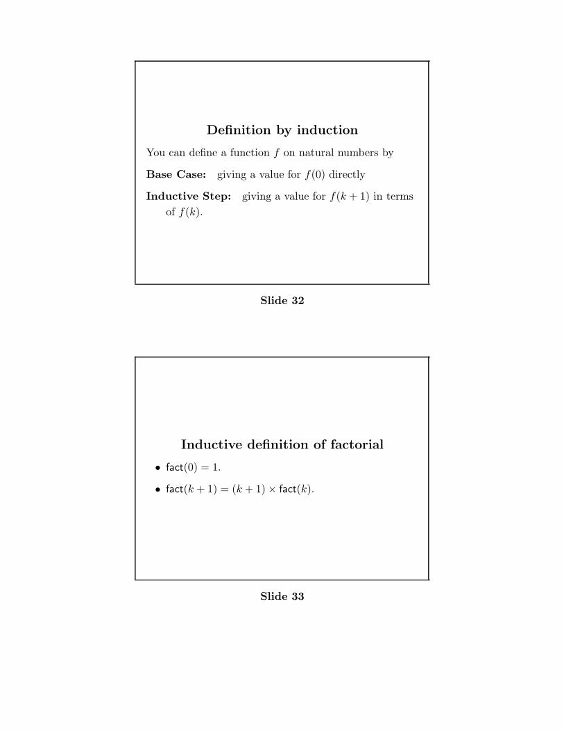
Definition by induction

You can define a function f on natural numbers by

Base Case: giving a value for f(0) directly

Inductive Step: giving a value for f(k + 1) in terms

of f(k).

Slide 32

Inductive definition of factorial

• fact(0) = 1.

• fact(k + 1) = (k + 1) × fact(k).

Slide 33

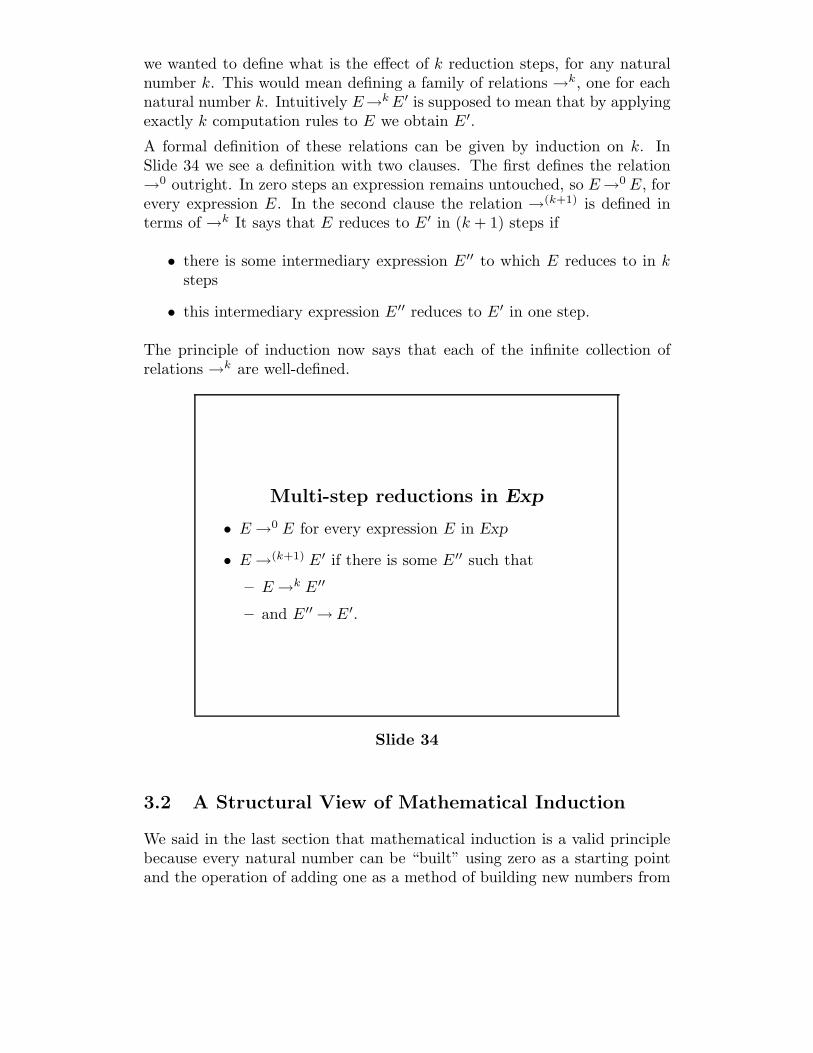
we wanted to define what is the effect of k reduction steps, for any naturalnumber k. This would mean defining a family of relations →k, one for eachnatural number k. Intuitively E→k E′ is supposed to mean that by applyingexactly k computation rules to E we obtain E′.

A formal definition of these relations can be given by induction on k. InSlide 34 we see a definition with two clauses. The first defines the relation→0 outright. In zero steps an expression remains untouched, so E →0 E, forevery expression E. In the second clause the relation →(k+1) is defined interms of →k It says that E reduces to E′ in (k + 1) steps if

• there is some intermediary expression E′′ to which E reduces to in ksteps

• this intermediary expression E′′ reduces to E′ in one step.

The principle of induction now says that each of the infinite collection ofrelations →k are well-defined.

Multi-step reductions in Exp

• E →0 E for every expression E in Exp

• E →(k+1) E′ if there is some E′′ such that

– E →k E′′

– and E′′ → E′.

Slide 34

3.2 A Structural View of Mathematical Induction

We said in the last section that mathematical induction is a valid principlebecause every natural number can be “built” using zero as a starting pointand the operation of adding one as a method of building new numbers from

old. We can turn mathematical induction into a form of structural inductionby viewing numbers as elements of the following grammar:

N ::= zero | succ(N).

Here succ, short for successor, should be thought of as the operation of addingone. Therefore zero represents 0, and 3 is represented by

succ(succ(succ(zero))).

With this view, it really is the case that a number is built by starting fromzero and repeatedly applying succ. Numbers, when thought of like this, arefinite, structured objects. The structure can be described as follows.

A number is either zero, which is indecomposable, or has the formsucc(N), where N is another number.

(We might refer to this N as a sub-number, since it is a substructure ofthe bigger number; but in this case that nomenclature is very unusual andclumsy.)

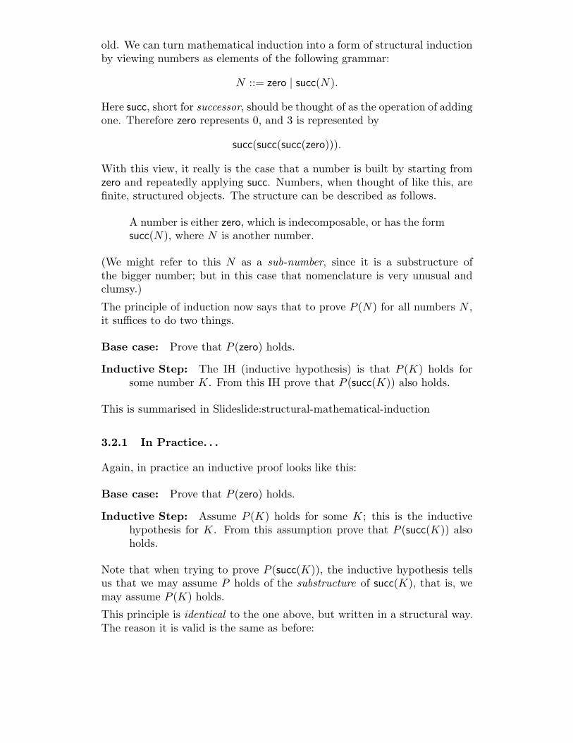
The principle of induction now says that to prove P (N) for all numbers N ,it suffices to do two things.

Base case: Prove that P (zero) holds.

Inductive Step: The IH (inductive hypothesis) is that P (K) holds forsome number K. From this IH prove that P (succ(K)) also holds.

This is summarised in Slideslide:structural-mathematical-induction

3.2.1 In Practice. . .

Again, in practice an inductive proof looks like this:

Base case: Prove that P (zero) holds.

Inductive Step: Assume P (K) holds for some K; this is the inductivehypothesis for K. From this assumption prove that P (succ(K)) alsoholds.

Note that when trying to prove P (succ(K)), the inductive hypothesis tellsus that we may assume P holds of the substructure of succ(K), that is, wemay assume P (K) holds.

This principle is identical to the one above, but written in a structural way.The reason it is valid is the same as before:

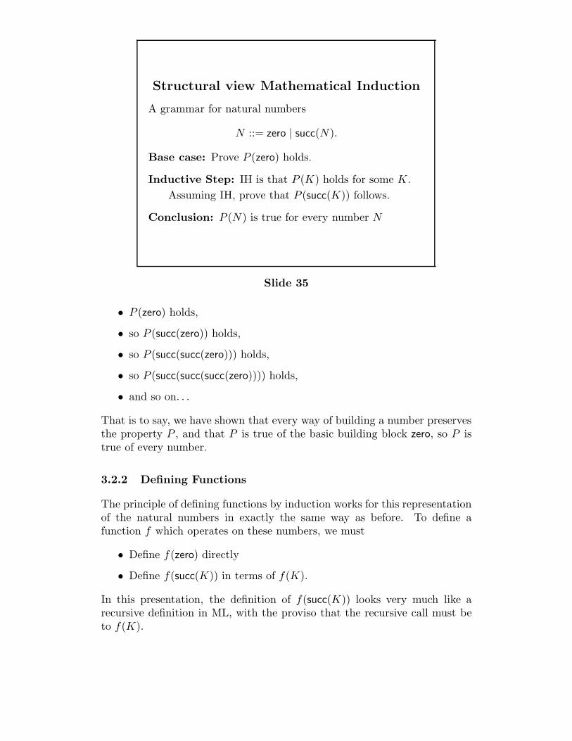
Structural view Mathematical Induction

A grammar for natural numbers

N ::= zero | succ(N).

Base case: Prove P (zero) holds.

Inductive Step: IH is that P (K) holds for some K.

Assuming IH, prove that P (succ(K)) follows.

Conclusion: P (N) is true for every number N

Slide 35

• P (zero) holds,

• so P (succ(zero)) holds,

• so P (succ(succ(zero))) holds,

• so P (succ(succ(succ(zero)))) holds,

• and so on. . .

That is to say, we have shown that every way of building a number preservesthe property P , and that P is true of the basic building block zero, so P istrue of every number.

3.2.2 Defining Functions

The principle of defining functions by induction works for this representationof the natural numbers in exactly the same way as before. To define afunction f which operates on these numbers, we must

• Define f(zero) directly

• Define f(succ(K)) in terms of f(K).

In this presentation, the definition of f(succ(K)) looks very much like arecursive definition in ML, with the proviso that the recursive call must beto f(K).

3.3 Structural Induction for Binary Trees

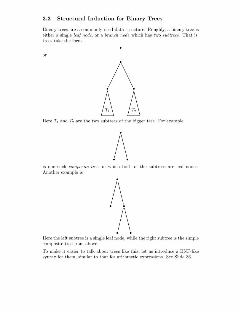
Binary trees are a commonly used data structure. Roughly, a binary tree iseither a single leaf node, or a branch node which has two subtrees. That is,trees take the form

or

T1 T2

Here T1 and T2 are the two subtrees of the bigger tree. For example,

is one such composite tree, in which both of the subtrees are leaf nodes.Another example is

Here the left subtree is a single leaf node, while the right subtree is the simplecomposite tree from above.

To make it easier to talk about trees like this, let us introduce a BNF-likesyntax for them, similar to that for arithmetic expressions. See Slide 36.

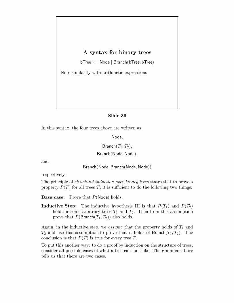
A syntax for binary trees

bTree ::= Node | Branch(bTree, bTree)

Note similarity with arithmetic expressions

Slide 36

In this syntax, the four trees above are written as

Node,

Branch(T1, T2),

Branch(Node, Node),

andBranch(Node, Branch(Node, Node))

respectively.

The principle of structural induction over binary trees states that to prove aproperty P (T ) for all trees T , it is sufficient to do the following two things:

Base case: Prove that P (Node) holds.

Inductive Step: The inductive hypothesis IH is that P (T1) and P (T2)hold for some arbitrary trees T1 and T2. Then from this assumptionprove that P (Branch(T1, T2)) also holds.

Again, in the inductive step, we assume that the property holds of T1 andT2 and use this assumption to prove that it holds of Branch(T1, T2). Theconclusion is that P (T ) is true for every tree T .

To put this another way: to do a proof by induction on the structure of trees,consider all possible cases of what a tree can look like. The grammar abovetells us that there are two cases.

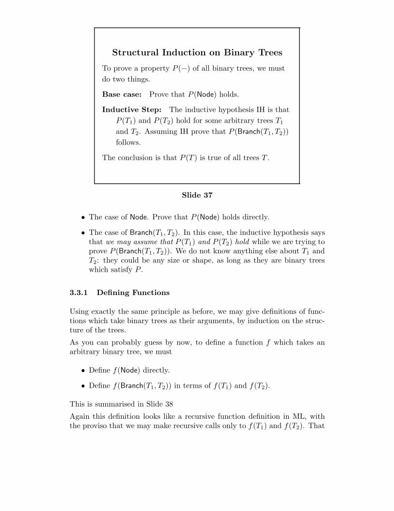
Structural Induction on Binary Trees

To prove a property P (−) of all binary trees, we must

do two things.

Base case: Prove that P (Node) holds.

Inductive Step: The inductive hypothesis IH is that

P (T1) and P (T2) hold for some arbitrary trees T1

and T2. Assuming IH prove that P (Branch(T1, T2))

follows.

The conclusion is that P (T ) is true of all trees T .

Slide 37

• The case of Node. Prove that P (Node) holds directly.

• The case of Branch(T1, T2). In this case, the inductive hypothesis saysthat we may assume that P (T1) and P (T2) hold while we are trying toprove P (Branch(T1, T2)). We do not know anything else about T1 andT2: they could be any size or shape, as long as they are binary treeswhich satisfy P .

3.3.1 Defining Functions

Using exactly the same principle as before, we may give definitions of func-tions which take binary trees as their arguments, by induction on the struc-ture of the trees.

As you can probably guess by now, to define a function f which takes anarbitrary binary tree, we must

• Define f(Node) directly.

• Define f(Branch(T1, T2)) in terms of f(T1) and f(T2).

This is summarised in Slide 38

Again this definition looks like a recursive function definition in ML, withthe proviso that we may make recursive calls only to f(T1) and f(T2). That

Defining functions over binary trees

To define a function f on binary trees we must

Base Case: give a value for f(Node) directly

Inductive Step: define f(Branch(T1, T2), using (if

necessary) f(T1) and f(T2).

f(T ) is then defined for every tree T .

Slide 38

is to say, the recursive calls must be with the immediate subtrees of the treewe are interested in.

Another way to think of such a function definition is that it says how tobuild up the value of f(T ) for any tree, in the same way that the tree isbuilt up. Since any tree can be built starting with some Nodes and puttingthings together using Branch(−,−), a definition like this lets us calculatef(T ) bit-by-bit.

3.3.2 Example

Here is an example of a pair of inductive definitions over trees, and a proofof a relationship between them.

We first define the function leaves which returns the number of leaf Nodes ina tree.

Base case: leaves(Node) = 1.

Inductive Step: leaves(Branch(T1, T2)) = leaves(T1) + leaves(T2).

We now define another function, branches, which counts the number ofBranch(−,−) nodes in a tree.

Base case: branches(Node) = 0.

Inductive Step: branches(Branch(T1, T2)) = branches(T1)+branches(T2)+1.

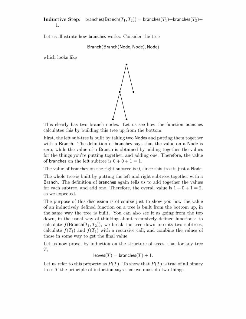
Let us illustrate how branches works. Consider the tree

Branch(Branch(Node, Node), Node)

which looks like

This clearly has two branch nodes. Let us see how the function branchescalculates this by building this tree up from the bottom.

First, the left sub-tree is built by taking two Nodes and putting them togetherwith a Branch. The definition of branches says that the value on a Node iszero, while the value of a Branch is obtained by adding together the valuesfor the things you’re putting together, and adding one. Therefore, the valueof branches on the left subtree is 0 + 0 + 1 = 1.

The value of branches on the right subtree is 0, since this tree is just a Node.

The whole tree is built by putting the left and right subtrees together with aBranch. The definition of branches again tells us to add together the valuesfor each subtree, and add one. Therefore, the overall value is 1 + 0 + 1 = 2,as we expected.

The purpose of this discussion is of course just to show you how the valueof an inductively defined function on a tree is built from the bottom up, inthe same way the tree is built. You can also see it as going from the topdown, in the usual way of thinking about recursively defined functions: tocalculate f(Branch(T1, T2)), we break the tree down into its two subtrees,calculate f(T1) and f(T2) with a recursive call, and combine the values ofthose in some way to get the final value.

Let us now prove, by induction on the structure of trees, that for any treeT ,

leaves(T ) = branches(T ) + 1.

Let us refer to this property as P (T ). To show that P (T ) is true of all binarytrees T the principle of induction says that we must do two things.

Base case: Prove that P (Node) is true; that is that leaves(Node) = branches(Node)+1.

Inductive Step: The inductive hypothesis IH is that P (T1) and P (T2) areboth true, for some T1 and T2. So we can assume IH, namely that

leaves(T1) = branches(T1) + 1

andleaves(T2) = branches(T2) + 1

From this assumption we have to derive P (Branch(T1, T2)), namelythat

leaves(Branch(T1, T2)) = branches(Branch(T1, T2)) + 1.

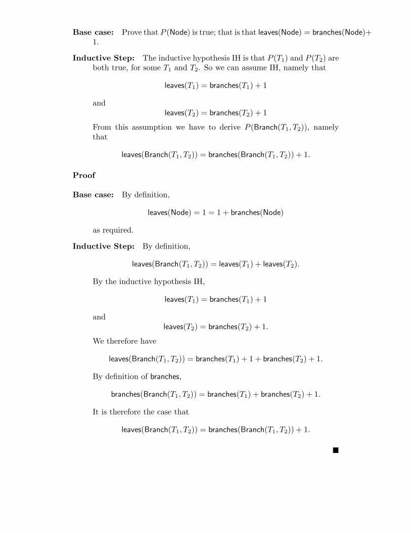
Proof

Base case: By definition,

leaves(Node) = 1 = 1 + branches(Node)

as required.

Inductive Step: By definition,

leaves(Branch(T1, T2)) = leaves(T1) + leaves(T2).

By the inductive hypothesis IH,

leaves(T1) = branches(T1) + 1

andleaves(T2) = branches(T2) + 1.

We therefore have

leaves(Branch(T1, T2)) = branches(T1) + 1 + branches(T2) + 1.

By definition of branches,

branches(Branch(T1, T2)) = branches(T1) + branches(T2) + 1.

It is therefore the case that

leaves(Branch(T1, T2)) = branches(Branch(T1, T2)) + 1.

!

3.4 Structural Induction over the Language of Expres-sions

The syntax of our illustrative language Exp of expressions also gives a collec-tion of structured, finite, but arbitrarily large objects over which inductionmay be used.

The syntax is given below.

E ∈ Exp ::= n | (E + E) | (E × E).

Recall that n ranges over the numerals 0, 1, 2 and so on. This means that inthis language there are in fact an infinite number of indecomposable expres-sions; contrast this with the cases above, where 0 is the only “indecomposablenatural number”, and Node is the only indecomposable binary tree.

In the previous examples, there was only one way of building new thingsfrom old: in the case of natural numbers, we built a new one from old byadding one (applying succ); and in the case of binary trees, we built a newtree from two old ones using Branch(−,−).

Here, on the other hand, we can build new expressions from old in two ways:using + and using ×.

The principle of induction for expressions reflects these differences as follows.If P is a property of expressions, then to prove that P (E) holds for any E,it suffices to do the following.

Base cases: Prove that P (n) holds for every numeral n.

Inductive Step: Here the inductive hypothesis IH is that P (E1) and P (E2)hold for some E1 and E2. Assuming IH we must show that bothP ((E1 + E2)) and P ((E1 × E2)) follow.

The conclusion will then be that P (E) is true of every expression E.

Again, this induction principle can be seen as a case-analysis: expressionscome in two forms:

• numerals, which cannot be decomposed, so we have to prove P (n)directly for each of them; and

• composite expressions (E1 + E2) and (E1 ×E2), which can be decom-posed into subexpressions E1 and E2. In this case, induction says thatwe may assume P (E1) and P (E2) when trying to prove P ((E1 + E2))and P ((E1 × E2)).

Structural Induction for Terms of Exp

To prove that property P (−) holds for all terms of Exp,

it suffices to prove

base cases: P (n) holds for all n, and

inductive step: The inductive hypothesis IH is that

P (E1) and P (E2) both hold for some arbitrary

expressions E1 and E2. From IH we must prove

that P (E1 + E2) and P (E1 × E2) follow.

Slide 39

3.4.1 Example

We shall prove by induction on the structure of expressions that for anyexpression E, there is some numeral n for which E⇓n. This property is callednormalisation: it says that all programs in our language have a final answeror so-called “normal form”. It goes hand in hand with another property,called determinacy, which we shall prove later.

Proposition 3 (Normalisation) For every expression E, there is some nsuch that E ⇓ n.

Proof By structural induction on E. The property P (E) of expressionswe wish to prove is

P (E) - there is some numeral n such that E ⇓ n.

The principle of structural induction says that to prove P (E) holds for everyexpression E we are required to establish two facts:

Base cases: P (n) holds for every numeral n.

For any numeral n, the axiom of the big-step semantics, (b-num), givesus that n ⇓ n, so the property is true of every n, as required.

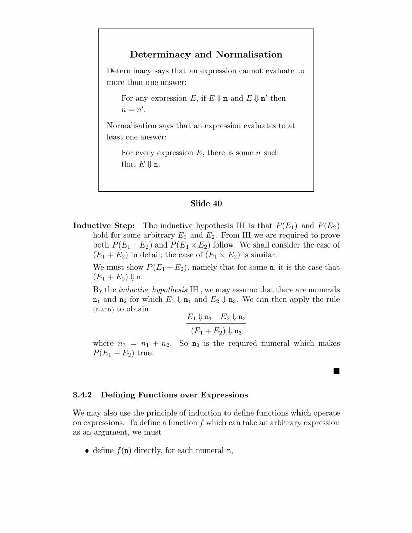
Determinacy and Normalisation

Determinacy says that an expression cannot evaluate to

more than one answer:

For any expression E, if E ⇓ n and E ⇓ n′ then

n = n′.

Normalisation says that an expression evaluates to at

least one answer:

For every expression E, there is some n such

that E ⇓ n.

Slide 40

Inductive Step: The inductive hypothesis IH is that P (E1) and P (E2)hold for some arbitrary E1 and E2. From IH we are required to proveboth P (E1 +E2) and P (E1 ×E2) follow. We shall consider the case of(E1 + E2) in detail; the case of (E1 × E2) is similar.

We must show P (E1 + E2), namely that for some n, it is the case that(E1 + E2) ⇓ n.

By the inductive hypothesis IH , we may assume that there are numeralsn1 and n2 for which E1 ⇓ n1 and E2 ⇓ n2. We can then apply the rule(b-add) to obtain

E1 ⇓ n1 E2 ⇓ n2

(E1 + E2) ⇓ n3

where n3 = n1 + n2. So n3 is the required numeral which makesP (E1 + E2) true.

!

3.4.2 Defining Functions over Expressions

We may also use the principle of induction to define functions which operateon expressions. To define a function f which can take an arbitrary expressionas an argument, we must

• define f(n) directly, for each numeral n,

• define f((E1 + E2)) in terms of f(E1) and f(E2), and

• define f((E1 × E2)) in terms of f(E1) and f(E2).

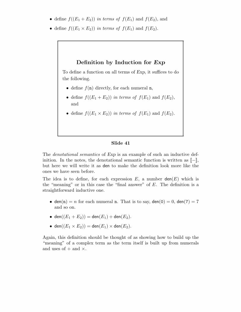
Definition by Induction for Exp

To define a function on all terms of Exp, it suffices to do

the following.

• define f(n) directly, for each numeral n,

• define f((E1 + E2)) in terms of f(E1) and f(E2),

and

• define f((E1 × E2)) in terms of f(E1) and f(E2).

Slide 41

The denotational semantics of Exp is an example of such an inductive def-inition. In the notes, the denotational semantic function is written as [[−]],but here we will write it as den to make the definition look more like theones we have seen before.

The idea is to define, for each expression E, a number den(E) which isthe “meaning” or in this case the “final answer” of E. The definition is astraightforward inductive one.

• den(n) = n for each numeral n. That is to say, den(0) = 0, den(7) = 7and so on.

• den((E1 + E2)) = den(E1) + den(E2).

• den((E1 × E2)) = den(E1) × den(E2).

Again, this definition should be thought of as showing how to build up the“meaning” of a complex term as the term itself is built up from numeralsand uses of + and ×.

3.5 Structural Induction over Derivations

The final example of a collection of finite, structured objects which we haveseen is the collection of proofs of statements E ⇓ n in the big-step semanticsof Exp. In general, an operational semantics given by axioms and proof rulesdefines a collection of proofs of this kind, and induction is available to us inreasoning about them.

To clarify the presentation, let us refer to such proofs as derivations in thissection.

Here is the derivation of (3 + (2 + 1)) ⇓ 6.

3 ⇓ 3

2 ⇓ 2 1 ⇓ 1

(2 + 1) ⇓ 3

(3 + (2 + 1)) ⇓ 6

This derivation has three key elements: the conclusion (3+ (2+ 1))⇓ 6, andthe two subderivations, which are

3 ⇓ 3

and

2 ⇓ 2 1 ⇓ 1

(2 + 1) ⇓ 3

We can think of a complex derivation like this as a structured object:

h1

D1

h2

D2

c

Here we see a derivation whose last rule is

h1 h2

c

where h1 and h2 are the hypotheses of the rule and c is the conclusion ofthe rule; c is also the conclusion of the whole derivation. Since the hypothe-ses themselves must be derived, there are subderivations D1 and D2 withconclusions h1 and h2.

The only derivations which do not decompose into a last rule and a collec-tion of subderivations are those which are simply axioms. Our principle ofinduction will therefore treat the axioms as the base cases, and the morecomplex proofs as the inductive step.

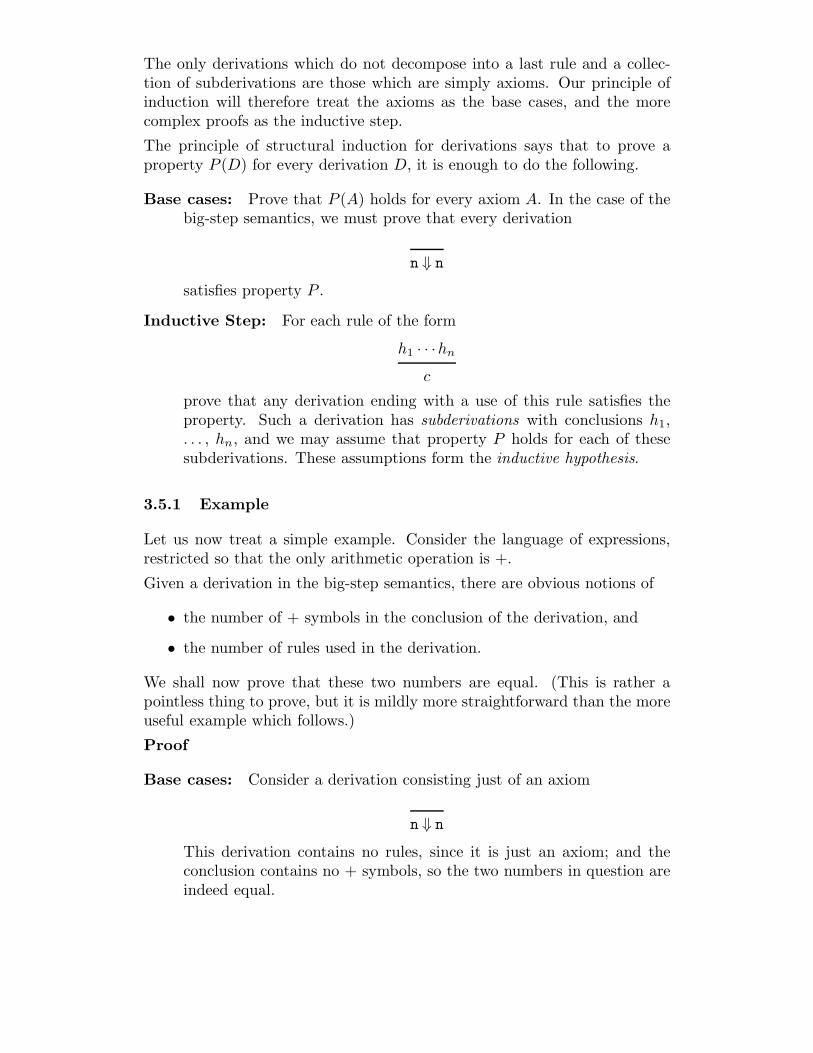
The principle of structural induction for derivations says that to prove aproperty P (D) for every derivation D, it is enough to do the following.

Base cases: Prove that P (A) holds for every axiom A. In the case of thebig-step semantics, we must prove that every derivation

n ⇓ n

satisfies property P .

Inductive Step: For each rule of the form

h1 · · ·hn

c

prove that any derivation ending with a use of this rule satisfies theproperty. Such a derivation has subderivations with conclusions h1,. . . , hn, and we may assume that property P holds for each of thesesubderivations. These assumptions form the inductive hypothesis.

3.5.1 Example

Let us now treat a simple example. Consider the language of expressions,restricted so that the only arithmetic operation is +.

Given a derivation in the big-step semantics, there are obvious notions of

• the number of + symbols in the conclusion of the derivation, and

• the number of rules used in the derivation.

We shall now prove that these two numbers are equal. (This is rather apointless thing to prove, but it is mildly more straightforward than the moreuseful example which follows.)

Proof

Base cases: Consider a derivation consisting just of an axiom

n ⇓ n

This derivation contains no rules, since it is just an axiom; and theconclusion contains no + symbols, so the two numbers in question areindeed equal.

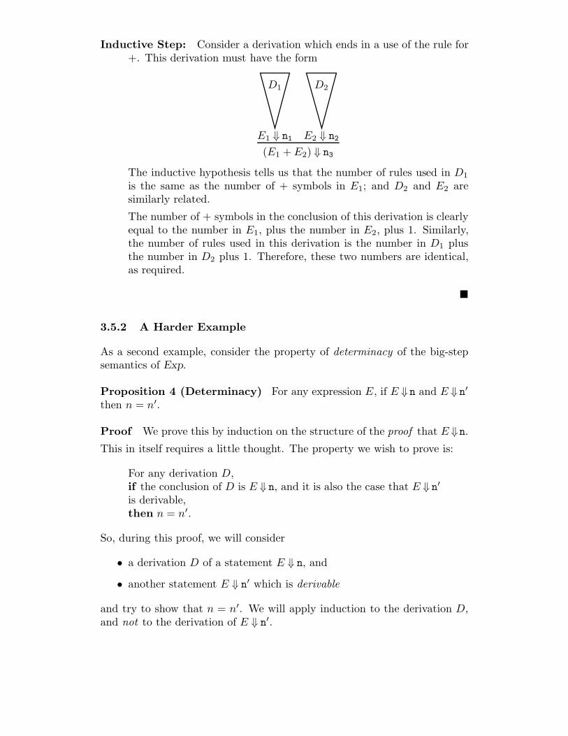
Inductive Step: Consider a derivation which ends in a use of the rule for+. This derivation must have the form

E1 ⇓ n1

D1

E2 ⇓ n2

D2

(E1 + E2) ⇓ n3

The inductive hypothesis tells us that the number of rules used in D1

is the same as the number of + symbols in E1; and D2 and E2 aresimilarly related.

The number of + symbols in the conclusion of this derivation is clearlyequal to the number in E1, plus the number in E2, plus 1. Similarly,the number of rules used in this derivation is the number in D1 plusthe number in D2 plus 1. Therefore, these two numbers are identical,as required.

!

3.5.2 A Harder Example

As a second example, consider the property of determinacy of the big-stepsemantics of Exp.

Proposition 4 (Determinacy) For any expression E, if E ⇓ n and E ⇓ n′

then n = n′.

Proof We prove this by induction on the structure of the proof that E ⇓n.

This in itself requires a little thought. The property we wish to prove is:

For any derivation D,if the conclusion of D is E ⇓ n, and it is also the case that E ⇓ n′

is derivable,then n = n′.

So, during this proof, we will consider

• a derivation D of a statement E ⇓ n, and

• another statement E ⇓ n′ which is derivable

and try to show that n = n′. We will apply induction to the derivation D,and not to the derivation of E ⇓ n′.

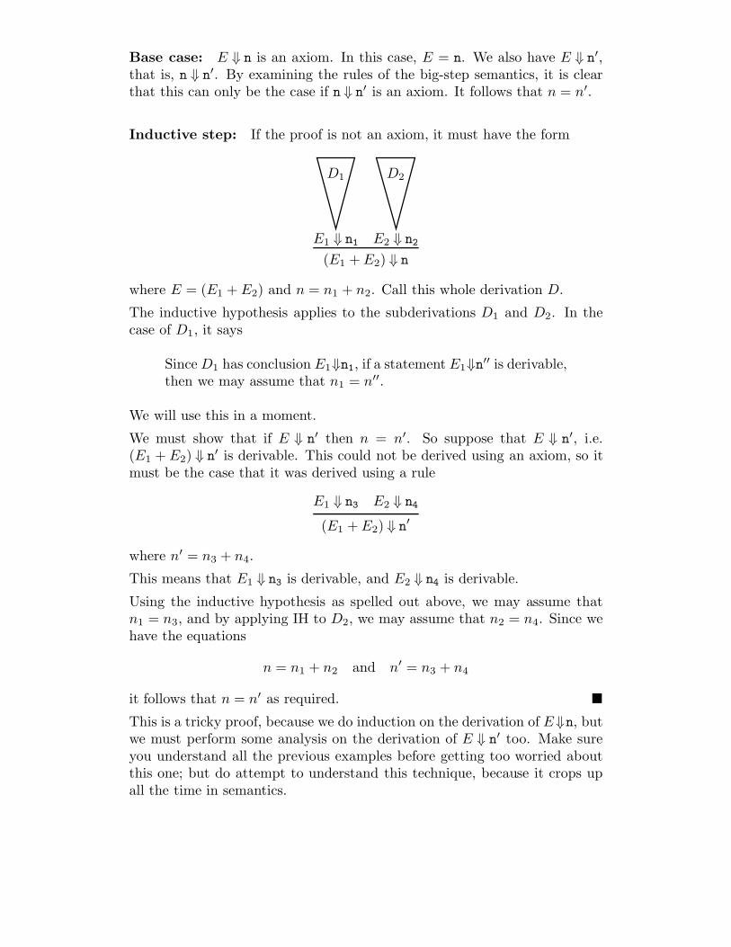
Base case: E ⇓ n is an axiom. In this case, E = n. We also have E ⇓ n′,that is, n ⇓ n′. By examining the rules of the big-step semantics, it is clearthat this can only be the case if n ⇓ n′ is an axiom. It follows that n = n′.

Inductive step: If the proof is not an axiom, it must have the form

E1 ⇓ n1

D1

E2 ⇓ n2

D2

(E1 + E2) ⇓ n

where E = (E1 + E2) and n = n1 + n2. Call this whole derivation D.

The inductive hypothesis applies to the subderivations D1 and D2. In thecase of D1, it says

Since D1 has conclusion E1⇓n1, if a statement E1⇓n′′ is derivable,then we may assume that n1 = n′′.

We will use this in a moment.

We must show that if E ⇓ n′ then n = n′. So suppose that E ⇓ n′, i.e.(E1 + E2) ⇓ n′ is derivable. This could not be derived using an axiom, so itmust be the case that it was derived using a rule

E1 ⇓ n3 E2 ⇓ n4

(E1 + E2) ⇓ n′

where n′ = n3 + n4.

This means that E1 ⇓ n3 is derivable, and E2 ⇓ n4 is derivable.

Using the inductive hypothesis as spelled out above, we may assume thatn1 = n3, and by applying IH to D2, we may assume that n2 = n4. Since wehave the equations

n = n1 + n2 and n′ = n3 + n4

it follows that n = n′ as required. !

This is a tricky proof, because we do induction on the derivation of E⇓n, butwe must perform some analysis on the derivation of E ⇓ n′ too. Make sureyou understand all the previous examples before getting too worried aboutthis one; but do attempt to understand this technique, because it crops upall the time in semantics.

3.6 Some proofs about the small-step semantics

We have seen how to use induction to prove simple facts about the big-stepsemantics of Exp. In this section we will see how to carry out similar proofsfor the small-step semantics, both to reassure ourselves that we’re on theright course and to make some intuitively obvious facts about our languageinto formal theorems.

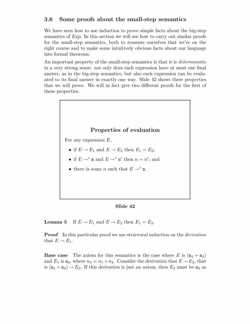
An important property of the small-step semantics is that it is deterministicin a very strong sense: not only does each expression have at most one finalanswer, as in the big-step semantics, but also each expression can be evalu-ated to its final answer in exactly one way. Slide 42 shows three propertiesthat we will prove. We will in fact give two different proofs for the first ofthese properties.

Properties of evaluation

For any expression E,

• if E → E1 and E → E2 then E1 = E2;

• if E →∗ n and E →∗ n′ then n = n′; and

• there is some n such that E →∗ n.

Slide 42

Lemma 5 If E → E1 and E → E2 then E1 = E2.

Proof In this particular proof we use structural induction on the derivationthat E → E1.

Base case The axiom for this semantics is the case where E is (n1 + n2)and E1 is n3, where n3 = n1 +n2. Consider the derivation that E→E2, thatis (n1 + n2)→E2. If this derivation is just an axiom, then E2 must be n3 as

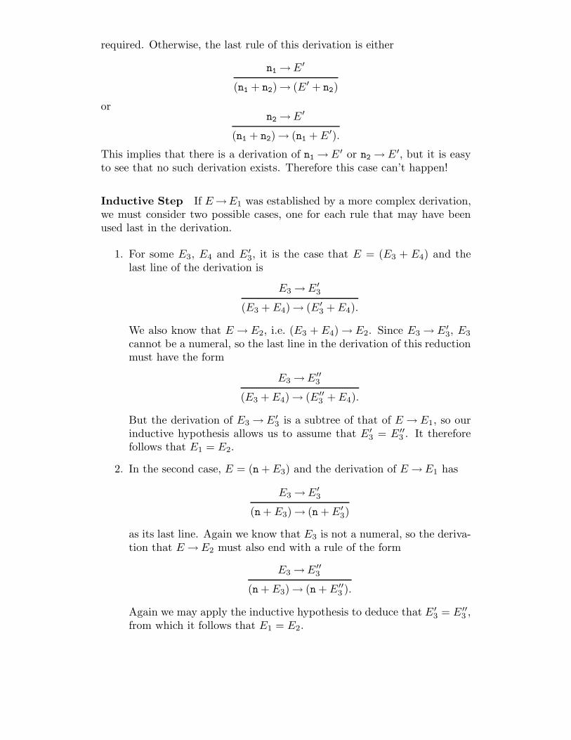
required. Otherwise, the last rule of this derivation is either

n1 → E′

(n1 + n2) → (E′ + n2)

orn2 → E′

(n1 + n2) → (n1 + E′).

This implies that there is a derivation of n1 → E′ or n2 → E′, but it is easyto see that no such derivation exists. Therefore this case can’t happen!

Inductive Step If E →E1 was established by a more complex derivation,we must consider two possible cases, one for each rule that may have beenused last in the derivation.

1. For some E3, E4 and E′3, it is the case that E = (E3 + E4) and the

last line of the derivation is

E3 → E′

3

(E3 + E4) → (E′3 + E4).

We also know that E → E2, i.e. (E3 + E4) → E2. Since E3 → E′3, E3

cannot be a numeral, so the last line in the derivation of this reductionmust have the form

E3 → E′′

3

(E3 + E4) → (E′′

3 + E4).

But the derivation of E3 → E′3 is a subtree of that of E → E1, so our

inductive hypothesis allows us to assume that E′3 = E′′

3 . It thereforefollows that E1 = E2.

2. In the second case, E = (n + E3) and the derivation of E → E1 has

E3 → E′

3

(n + E3) → (n + E′

3)

as its last line. Again we know that E3 is not a numeral, so the deriva-tion that E → E2 must also end with a rule of the form

E3 → E′′

3

(n + E3) → (n + E′′

3 ).

Again we may apply the inductive hypothesis to deduce that E′3 = E′′

3 ,from which it follows that E1 = E2.

!

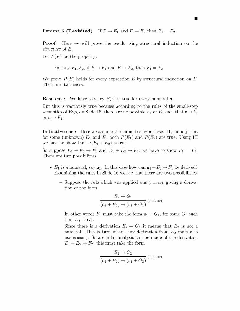
Lemma 5 (Revisited) If E → E1 and E → E2 then E1 = E2.

Proof Here we will prove the result using structural induction on thestructure of E.

Let P (E) be the property:

For any F1, F2, if E → F1 and E → F2, then F1 = F2

We prove P (E) holds for every expression E by structural induction on E.There are two cases.

Base case We have to show P (n) is true for every numeral n.

But this is vacuously true because according to the rules of the small-stepsemantics of Exp, on Slide 16, there are no possible F1 or F2 such that n→F1

or n→ F2.

Inductive case Here we assume the inductive hypothesis IH, namely thatfor some (unknown) E1 and E2 both P (E1) and P (E2) are true. Using IHwe have to show that P (E1 + E2) is true.

So suppose E1 + E2 → F1 and E1 + E2 → F2; we have to show F1 = F2.There are two possibilities.

• E1 is a numeral, say n1. In this case how can n1 +E2 →F1 be derived?Examining the rules in Slide 16 we see that there are two possibilities.

– Suppose the rule which was applied was (s-right), giving a deriva-tion of the form

E2 → G1(s-right)

(n1 + E2) → (n1 + G1)

In other words F1 must take the form n1 + G1, for some G1 suchthat E2 → G1.

Since there is a derivation E2 → G1 it means that E2 is not anumeral. This is turn means any derivation from E2 must alsouse (s-right). So a similar analysis can be made of the derivationE1 + E2 → F2; this must take the form

E2 → G2(s-right)

(n1 + E2) → (n1 + G2)

where F2 is n1 + G2.

But now we can use part of the inductive hypothesis, namelyP (E2); this tells us that G1 = G2. From this it follows thatF1 = F2.

– The second possibility is that n1 + E2 → F1 is derived by an ap-plication of the rule (s-add). So E2 must be a numeral, say n2 andso F1 is also a numeral, n3, where n1 + n2 = n3.

Now looking at the second derivation n1+E2→F2, since E2 is thenumeral n2, again the only possible rule which can be applied is(s-add), with the result that F2 is also n3; in other words, F1 = F2.

• So let us suppose that E1 is not a numeral. Here, what rules fromSlide 16 can be used to infer E1 + E2 → F1? The rules (s-right) and(s-add) require that E1 be a numeral. So the only possibility is (s-left),giving a derivation of the form the form

E1 → G1(s-right)

(E1 + E2) → (G1 + E2)

So F1 must be of the form G1 + E2 for some G1 such that E1 → G1.

A similar analysis gives that F2 must also be of the form G2 + E2 forsome G2 such that E1 → G2.

Now we can apply P (E1), which is part of the inductive hypothesis, toobtain that G1 = G2. It follows that F1 = F2.

!

This result says that the one-step relation is deterministic. Let us now seehow from this we can prove that there can be at most one final answer.First we show that the k-step reduction relation, defined in Slide 34, is alsodeterministic.

Corollary 6 For every natural number k and every expression E, if E →k

E1 and E →k E2 then E1 = E2.

Proof We prove this by mathematical induction on the natural number k.So let P (k) be the statement

E →k E1 and E →k E2 implies E1 = E2

By mathematical induction to prove P (n) holds for every n we need toestablish two facts.

Base case Here we establish P (0), namely that if E →0 E1 and E →0 E2

then E1 = E2.

But this is trivial. Looking at the definition of →k in Slide 34 we see thatthe only possibility for E1 and E2 is that they are E itself, and thereforemust be equal.

Inductive case Here we assume the inductive hypothesis, namely P (k).From this we must prove P (k+1), namely that if E→(k+1)E1 and E→(k+1)E2

then E1 = E2.

Again looking at the definition of →(k+1) in Slide 34 we know that theremust exist some expressions E′

1 and E′2 such that

E →k E′

1 → E1

E →k E′

2 → E2

But the inductive hypothesis gives that E′1 = E′

2, and the determinism of theone-step relation, proved in the previous Lemma, gives the required E1 = E2.

!

This corollary leads directly to the determinacy of the final result.

Lemma 7 If E →∗ n and E →∗ n′ then n = n′.

Proof The statement E →∗ n means that E reduces to n in some finitenumber of steps. So there is some natural number k1 such that E →k1 n1.Similarly we have some k2 such that E →k2 n2. Now either k1 ≤ k2 ork2 ≤ k1. Let us assume the former; the proof in the latter case is completelysymmetric. Then these derivations take the form

E →k1 n1

E →k1 E′ →(k2−k1) n2

for some intermediary expression E′.

But by the previous Corollary E′ must be the same as n. According to therules in Slide 16 no reductions can be made from numerals. So the reductionE′ →(k2−k1) n2 must be the trivial one n1 →0 n2. In other words n1 = n2. !

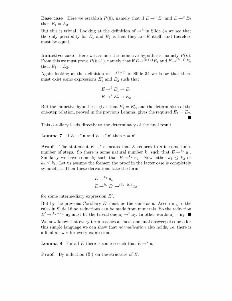
We now know that every term reaches at most one final answer; of course forthis simple language we can show that normalisation also holds, i.e. there isa final answer for every expression.

Lemma 8 For all E there is some n such that E →∗ n.

Proof By induction (!!!) on the structure of E.

Base Case E is a numeral n. Then n→∗ n as required.

Inductive Step E is (E1 + E2). By the inductive hypothesis, we havenumbers n1 and n2 such that E1 →∗ n1 and E2 →∗ n2. For each step in thereduction

E1 → E′

1 → E′′

1 · · ·→ n1

applying the rule for reducing the left argument of an addition gives

(E1 + E2) → (E′

1 + E2) → (E′′

1 + E2) · · ·→ (n1 + E2).

Applying the other rule to the sequence for E2 →∗ n2 allows us to deducethat

(n1 + E2) →∗ (n1 + n2) → n3

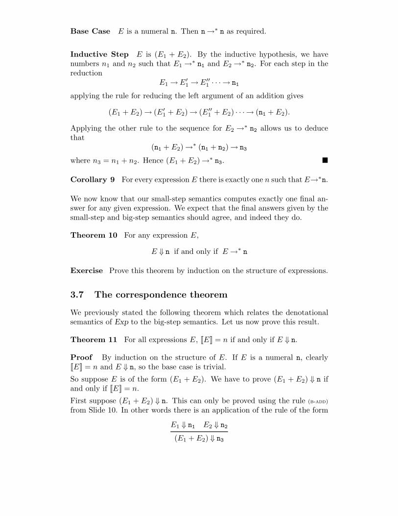
where n3 = n1 + n2. Hence (E1 + E2) →∗ n3. !

Corollary 9 For every expression E there is exactly one n such that E→∗n.

We now know that our small-step semantics computes exactly one final an-swer for any given expression. We expect that the final answers given by thesmall-step and big-step semantics should agree, and indeed they do.

Theorem 10 For any expression E,

E ⇓ n if and only if E →∗ n

Exercise Prove this theorem by induction on the structure of expressions.

3.7 The correspondence theorem

We previously stated the following theorem which relates the denotationalsemantics of Exp to the big-step semantics. Let us now prove this result.

Theorem 11 For all expressions E, [[E]] = n if and only if E ⇓ n.

Proof By induction on the structure of E. If E is a numeral n, clearly[[E]] = n and E ⇓ n, so the base case is trivial.

So suppose E is of the form (E1 + E2). We have to prove (E1 + E2) ⇓ n ifand only if [[E]] = n.

First suppose (E1 + E2) ⇓ n. This can only be proved using the rule (b-add)

from Slide 10. In other words there is an application of the rule of the form

E1 ⇓ n1 E2 ⇓ n2

(E1 + E2) ⇓ n3

for some numbers n1, n2 such that n3 = n1+n2. By the inductive hypothesis,[[Ei]] = ni for i = 1, 2, and therefore

[[E1]] + [[E2]] = n1 + n2 = n3.

Conversely suppose [[E1]] + [[E2]] = n for some number n. Looking up thedefinition of the denotational semantics of Exp in Slide 19 we see that theremust be two numbers n1 and n2, namely [[E1]] and [[E2]] respectively, suchthat n = n1+n2. Since [[Ei]] = ni we can apply structural induction to obtainEi ⇓ni and an application of the rule (b-add) gives the required (E1 +E2)⇓n.

!

To sum up the results of this chapter, we have seen three different semanticsfor the language Exp, a denotational one, given in Slide 19, and two opera-tional ones, in Slide 10 and Slide 16. We now know that these three differentviews actually coincide. For every expression E

[[E]] = n if and only if E ⇓ n if and only if E →∗ n

4 A Simple Programming Language

Let us now consider a “proper” programming language. The language Whileof while-programs has a grammar consisting of three syntax-categories: ex-pressions as before, which we now denote with N to indicate that they arenumeric expressions; booleans, which are very similar to expressions butrepresent truth-values rather than numbers; and commands, which are im-perative statements which affect the store of the computer. The grammar isgiven on Slide 43.

The collection of expressions now includes a class x of mutable variables;here x ranges over some fixed, infinite set of identifiers. The expression x isintended to mean “the value currently stored in x”. The intended meaningof the commands should be obvious to anyone familiar with imperative pro-gramming; we use the syntax x := E for the assignment statement, whichevaluates E and stores the result in x.

Abstract Syntax A reminder: we always deal with abstract syntax, eventhough the grammar above looks a bit like the kind of concrete syntax youmight type in to a computer. So, we’re really dealing with trees built upout of the term-forming operators given above. The operators we have forcommands are:

• assignment, which takes a variable and an expression and gives a com-mand, written x := E

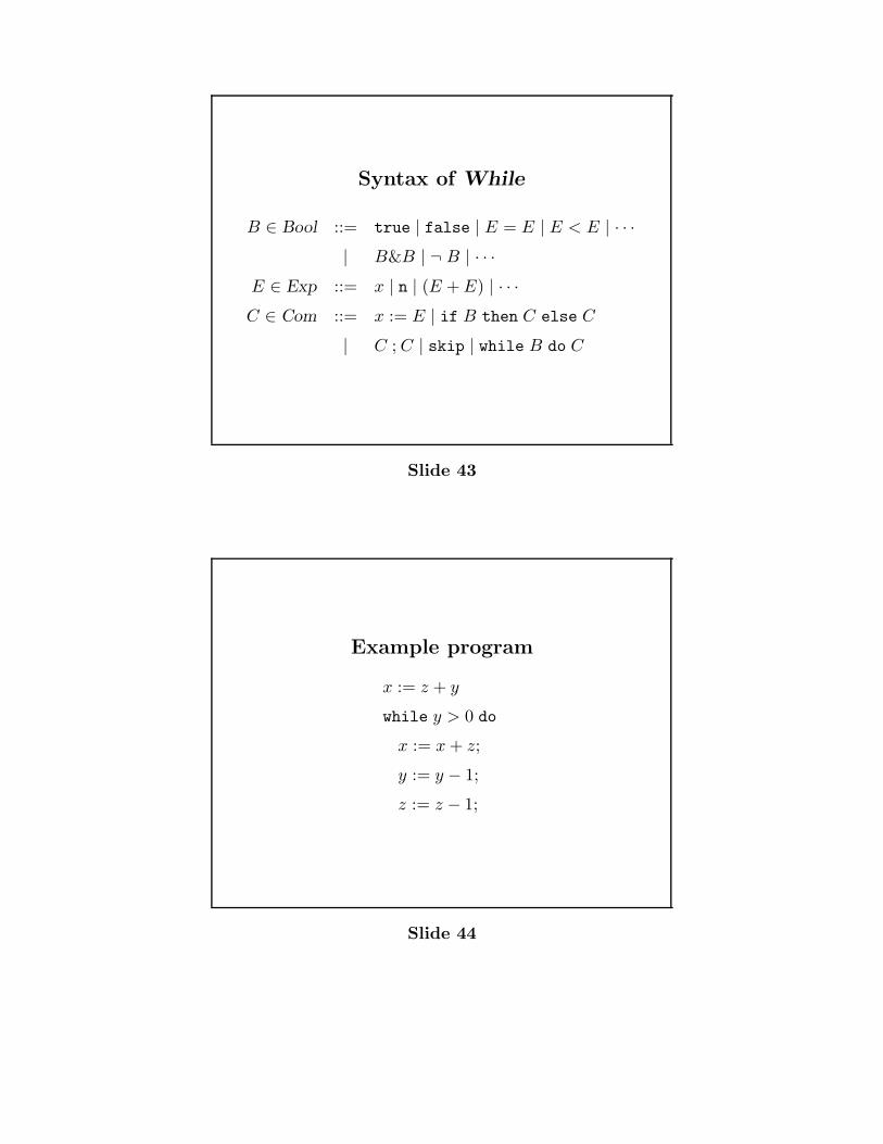
Syntax of While

B ∈ Bool ::= true | false | E = E | E < E | · · ·

| B&B | ¬ B | · · ·

E ∈ Exp ::= x | n | (E + E) | · · ·

C ∈ Com ::= x := E | if B then C else C

| C ; C | skip | while B do C

Slide 43

Example program

x := z + y

while y > 0 do

x := x + z;

y := y − 1;

z := z − 1;

Slide 44

• the conditional, taking a boolean and two commands and yielding acommand, written if B then C1 else C2

• sequential composition, which takes two commands and yields a com-mand, written C1 ; C2 (note that the semicolon here is an operatorjoining two commands into one, and not just a piece of punctuation atthe end of a command)

• the “do nothing” constant skip

• the loop constructor, which takes a boolean and a command and yieldsa command, written while B do C.

4.1 Small-step Semantics

How should we give a small-step semantics to While? In particular, how dowe evaluate a variable:

x → ?

or an assignmentx := n→ ?

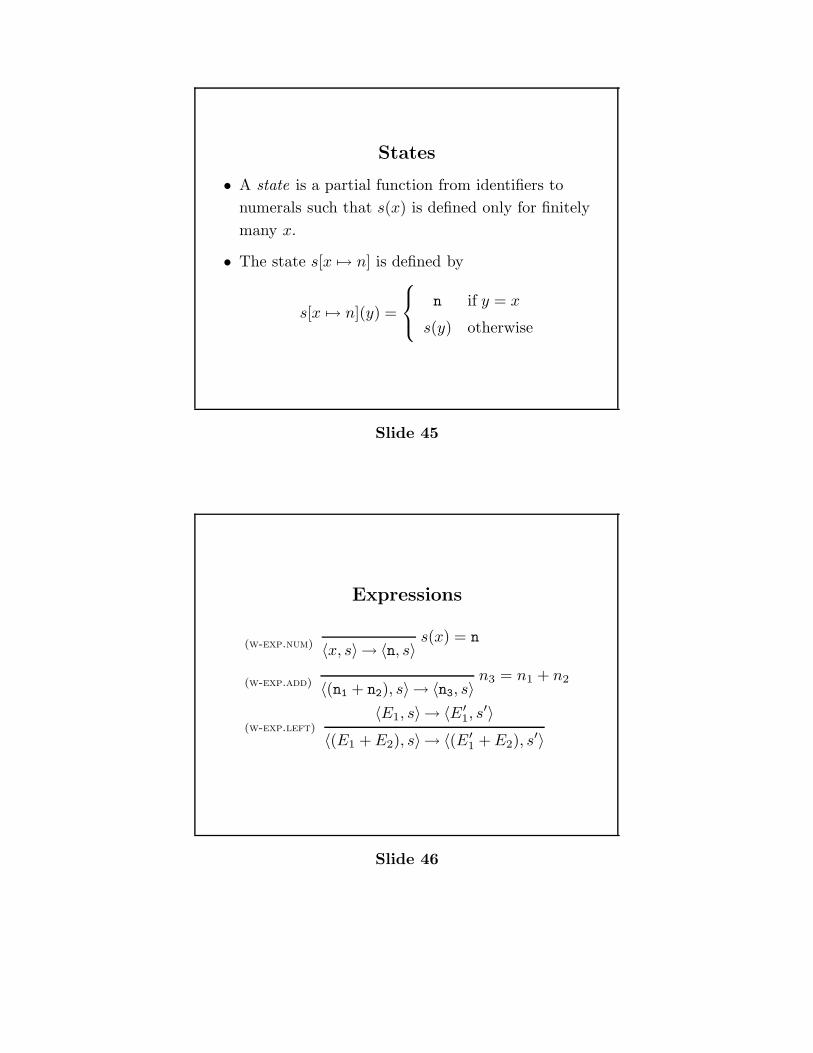
Obviously, we need some more information, about the state of the machine’smemory. Slide 45 gives the definition of a state suitable for modelling While.Intuitively, a state s tells us what, if anything, is stored in the memorylocation corresponding to each identifier of the language, and s[x ,→ n] is thestate s updated so that the location corresponding to x contains n.

Our small-step semantics will therefore be concerned with programs togetherwith their store, so we define a relation of the form

〈P, s〉→ 〈P ′, s′〉.

Expressions and Booleans Expressions and booleans do not present anydifficulty. The only really new kind of expression is the variable. Its semanticsinvolves fetching the appropriate value from the store. The correspondingrule, and some of the old rules updated for the new language, are shown inSlide 46.

Exercise Write down the other rules for expressions, and all the rules forbooleans.

States

• A state is a partial function from identifiers to

numerals such that s(x) is defined only for finitely

many x.

• The state s[x ,→ n] is defined by

s[x ,→ n](y) =

n if y = x

s(y) otherwise

Slide 45

Expressions

(w-exp.num)s(x) = n

〈x, s〉 → 〈n, s〉

(w-exp.add)n3 = n1 + n2

〈(n1 + n2), s〉 → 〈n3, s〉

(w-exp.left)〈E1, s〉 → 〈E′

1, s′〉

〈(E1 + E2), s〉 → 〈(E′

1 + E2), s′〉

Slide 46

Commands The rules defining the semantics for commands are different:they will alter the store in interesting ways. Intuitively, we want our rules toshow how commands update the store, and we will know that a commandhas finished its work when it reduces to skip. We shall now consider eachkind of command in turn and write down the appropriate rules.

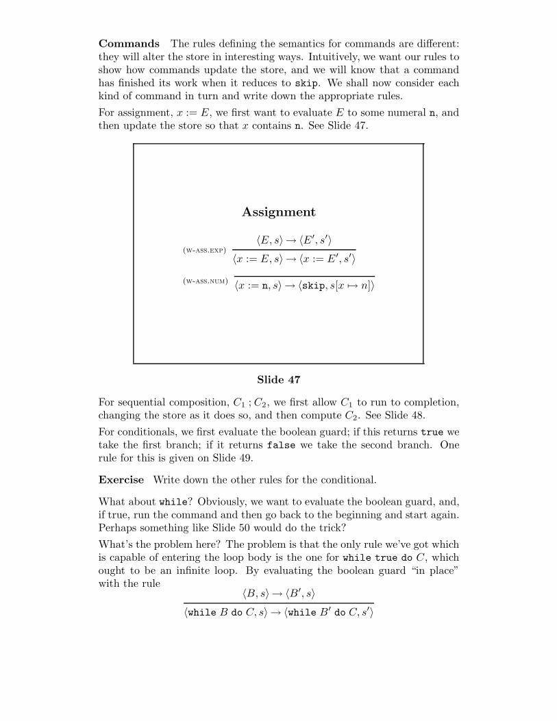
For assignment, x := E, we first want to evaluate E to some numeral n, andthen update the store so that x contains n. See Slide 47.

Assignment

(w-ass.exp)〈E, s〉→ 〈E′, s′〉

〈x := E, s〉 → 〈x := E′, s′〉

(w-ass.num) 〈x := n, s〉 → 〈skip, s[x ,→ n]〉

Slide 47

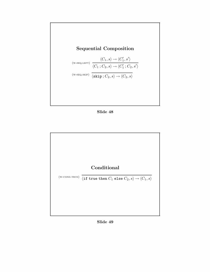
For sequential composition, C1 ; C2, we first allow C1 to run to completion,changing the store as it does so, and then compute C2. See Slide 48.

For conditionals, we first evaluate the boolean guard; if this returns true wetake the first branch; if it returns false we take the second branch. Onerule for this is given on Slide 49.

Exercise Write down the other rules for the conditional.

What about while? Obviously, we want to evaluate the boolean guard, and,if true, run the command and then go back to the beginning and start again.Perhaps something like Slide 50 would do the trick?

What’s the problem here? The problem is that the only rule we’ve got whichis capable of entering the loop body is the one for while true do C, whichought to be an infinite loop. By evaluating the boolean guard “in place”with the rule

〈B, s〉→ 〈B′, s〉

〈while B do C, s〉→ 〈while B′ do C, s′〉

Sequential Composition

(w-seq.left)〈C1, s〉 → 〈C′

1, s′〉

〈C1 ; C2, s〉 → 〈C′1 ; C2, s

′〉

(w-seq.skip) 〈skip ; C2, s〉 → 〈C2, s〉

Slide 48

Conditional

(w-cond.true) 〈if true then C1 else C2, s〉 → 〈C1, s〉

Slide 49

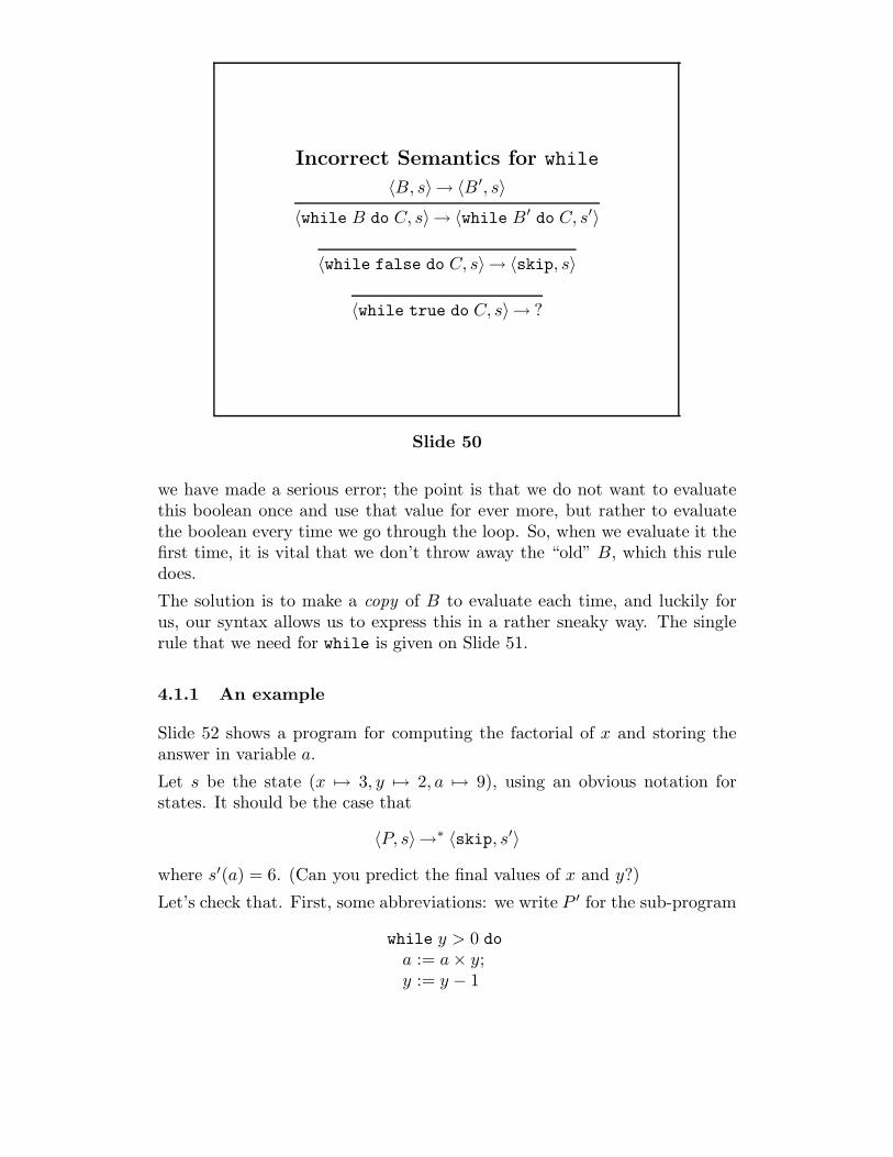
Incorrect Semantics for while

〈B, s〉→ 〈B′, s〉

〈while B do C, s〉→ 〈while B′ do C, s′〉

〈while false do C, s〉→ 〈skip, s〉

〈while true do C, s〉→ ?

Slide 50

we have made a serious error; the point is that we do not want to evaluatethis boolean once and use that value for ever more, but rather to evaluatethe boolean every time we go through the loop. So, when we evaluate it thefirst time, it is vital that we don’t throw away the “old” B, which this ruledoes.

The solution is to make a copy of B to evaluate each time, and luckily forus, our syntax allows us to express this in a rather sneaky way. The singlerule that we need for while is given on Slide 51.

4.1.1 An example

Slide 52 shows a program for computing the factorial of x and storing theanswer in variable a.

Let s be the state (x ,→ 3, y ,→ 2, a ,→ 9), using an obvious notation forstates. It should be the case that

〈P, s〉→∗ 〈skip, s′〉

where s′(a) = 6. (Can you predict the final values of x and y?)

Let’s check that. First, some abbreviations: we write P ′ for the sub-program

while y > 0 doa := a × y;y := y − 1

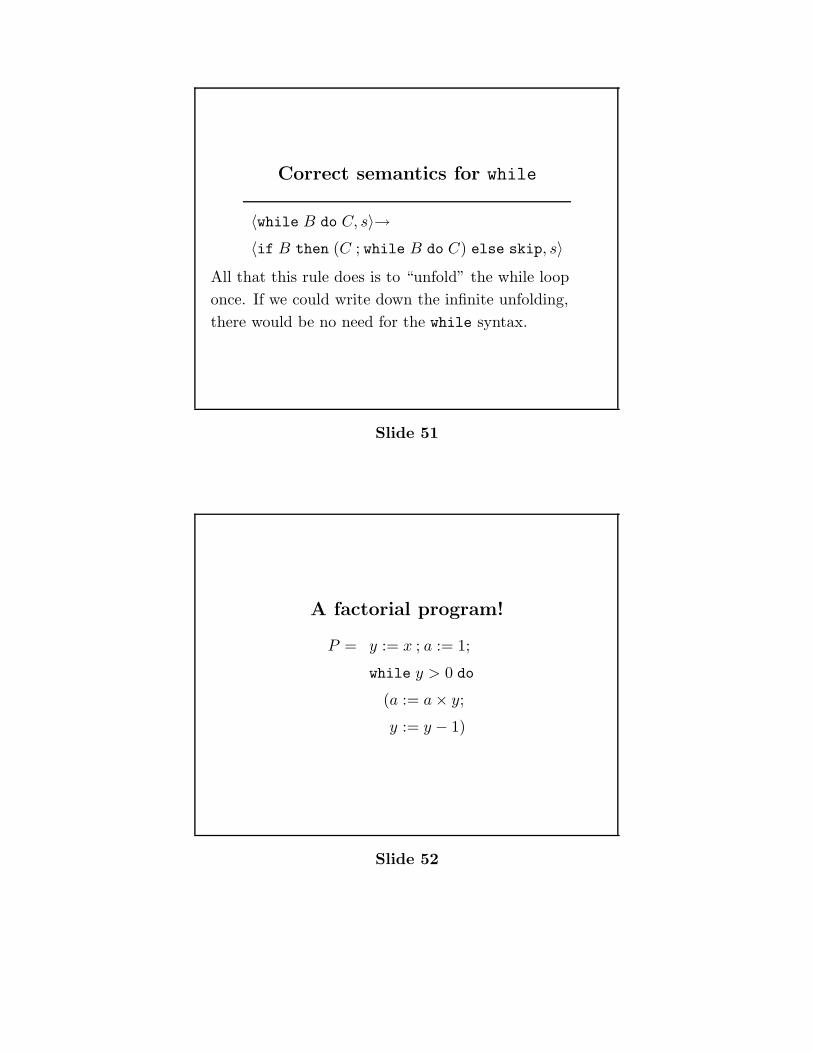
Correct semantics for while

〈while B do C, s〉→

〈if B then (C ; while B do C) else skip, s〉

All that this rule does is to “unfold” the while loop

once. If we could write down the infinite unfolding,

there would be no need for the while syntax.

Slide 51

A factorial program!

P = y := x ; a := 1;

while y > 0 do

(a := a × y;

y := y − 1)

Slide 52

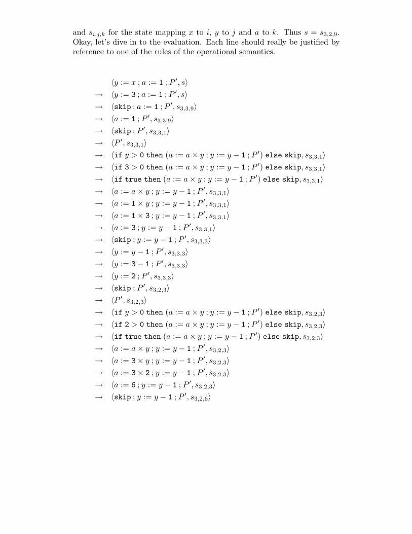
and si,j,k for the state mapping x to i, y to j and a to k. Thus s = s3,2,9.Okay, let’s dive in to the evaluation. Each line should really be justified byreference to one of the rules of the operational semantics.

〈y := x ; a := 1 ; P ′, s〉

→ 〈y := 3 ; a := 1 ; P ′, s〉

→ 〈skip ; a := 1 ; P ′, s3,3,9〉

→ 〈a := 1 ; P ′, s3,3,9〉

→ 〈skip ; P ′, s3,3,1〉

→ 〈P ′, s3,3,1〉

→ 〈if y > 0 then (a := a × y ; y := y − 1 ; P ′) else skip, s3,3,1〉

→ 〈if 3 > 0 then (a := a × y ; y := y − 1 ; P ′) else skip, s3,3,1〉

→ 〈if true then (a := a × y ; y := y − 1 ; P ′) else skip, s3,3,1〉

→ 〈a := a × y ; y := y − 1 ; P ′, s3,3,1〉

→ 〈a := 1× y ; y := y − 1 ; P ′, s3,3,1〉

→ 〈a := 1× 3 ; y := y − 1 ; P ′, s3,3,1〉

→ 〈a := 3 ; y := y − 1 ; P ′, s3,3,1〉

→ 〈skip ; y := y − 1 ; P ′, s3,3,3〉

→ 〈y := y − 1 ; P ′, s3,3,3〉

→ 〈y := 3− 1 ; P ′, s3,3,3〉

→ 〈y := 2 ; P ′, s3,3,3〉

→ 〈skip ; P ′, s3,2,3〉

→ 〈P ′, s3,2,3〉

→ 〈if y > 0 then (a := a × y ; y := y − 1 ; P ′) else skip, s3,2,3〉

→ 〈if 2 > 0 then (a := a × y ; y := y − 1 ; P ′) else skip, s3,2,3〉

→ 〈if true then (a := a × y ; y := y − 1 ; P ′) else skip, s3,2,3〉

→ 〈a := a × y ; y := y − 1 ; P ′, s3,2,3〉

→ 〈a := 3× y ; y := y − 1 ; P ′, s3,2,3〉

→ 〈a := 3× 2 ; y := y − 1 ; P ′, s3,2,3〉

→ 〈a := 6 ; y := y − 1 ; P ′, s3,2,3〉

→ 〈skip ; y := y − 1 ; P ′, s3,2,6〉

→ 〈y := y − 1 ; P ′, s3,2,6〉

→ 〈y := 2− 1 ; P ′, s3,2,6〉

→ 〈y := 1 ; P ′, s3,2,6〉

→ 〈skip ; P ′, s3,1,6〉

→ 〈P ′, s3,1,6〉

→ 〈if y > 0 then (a := a × y ; y := y − 1 ; P ′) else skip, s3,1,6〉

→ 〈if 1 > 0 then (a := a × y ; y := y − 1 ; P ′) else skip, s3,1,6〉

→ 〈if true then (a := a × y ; y := y − 1 ; P ′) else skip, s3,1,6〉

→ 〈a := a × y ; y := y − 1 ; P ′, s3,1,6〉

→ 〈a := 6× y ; y := y − 1 ; P ′, s3,1,6〉

→ 〈a := 6× 1 ; y := y − 1 ; P ′, s3,1,6〉

→ 〈a := 6 ; y := y − 1 ; P ′, s3,1,6〉

→ 〈skip ; y := y − 1 ; P ′, s3,1,6〉

→ 〈y := y − 1 ; P ′, s3,1,6〉

→ 〈y := 1− 1 ; P ′, s3,1,6〉

→ 〈y := 0 ; P ′, s3,1,6〉

→ 〈skip ; P ′, s3,0,6〉

→ 〈P ′, s3,0,6〉

→ 〈if y > 0 then (a := a × y ; y := y − 1 ; P ′) else skip, s3,0,6〉

→ 〈if 0 > 0 then (a := a × y ; y := y − 1 ; P ′) else skip, s3,0,6〉

→ 〈if false then (a := a × y ; y := y − 1 ; P ′) else skip, s3,0,6〉

→ 〈skip, s3,0,6〉.

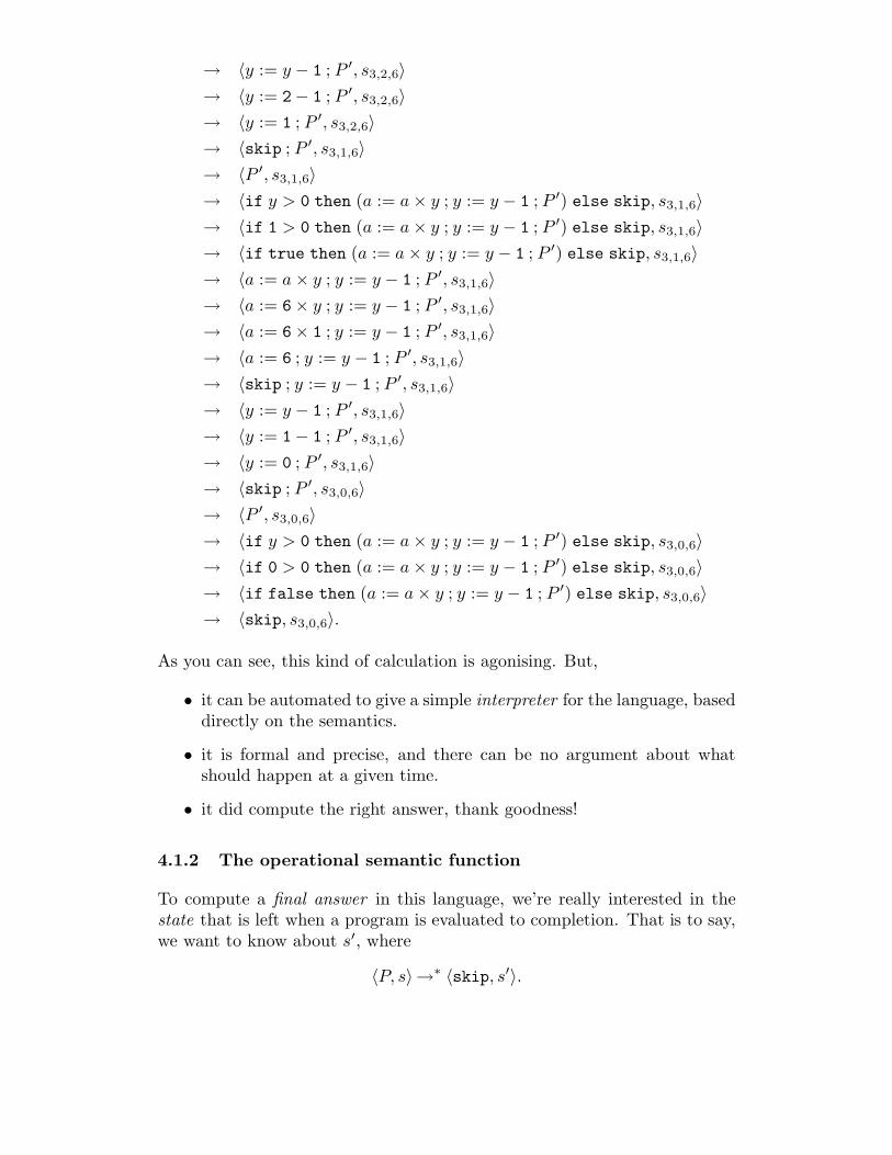
As you can see, this kind of calculation is agonising. But,

• it can be automated to give a simple interpreter for the language, baseddirectly on the semantics.

• it is formal and precise, and there can be no argument about whatshould happen at a given time.

• it did compute the right answer, thank goodness!

4.1.2 The operational semantic function

To compute a final answer in this language, we’re really interested in thestate that is left when a program is evaluated to completion. That is to say,we want to know about s′, where

〈P, s〉→∗ 〈skip, s′〉.

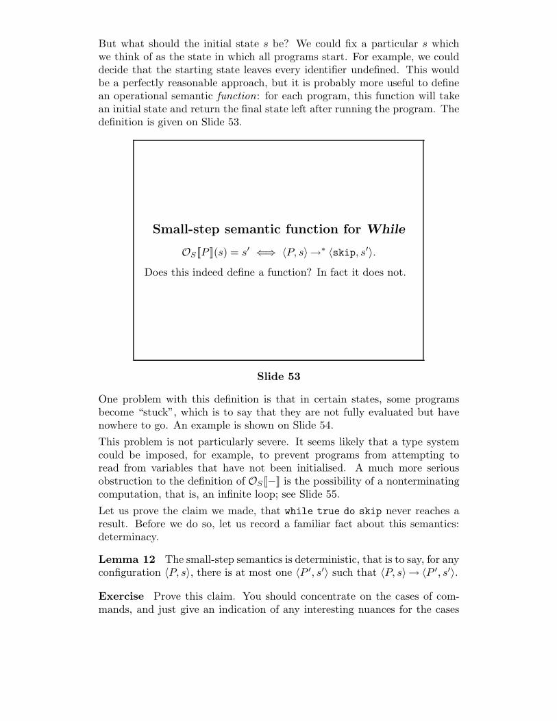
But what should the initial state s be? We could fix a particular s whichwe think of as the state in which all programs start. For example, we coulddecide that the starting state leaves every identifier undefined. This wouldbe a perfectly reasonable approach, but it is probably more useful to definean operational semantic function: for each program, this function will takean initial state and return the final state left after running the program. Thedefinition is given on Slide 53.

Small-step semantic function for While

OS [[P ]](s) = s′ ⇐⇒ 〈P, s〉→∗ 〈skip, s′〉.

Does this indeed define a function? In fact it does not.

Slide 53

One problem with this definition is that in certain states, some programsbecome “stuck”, which is to say that they are not fully evaluated but havenowhere to go. An example is shown on Slide 54.

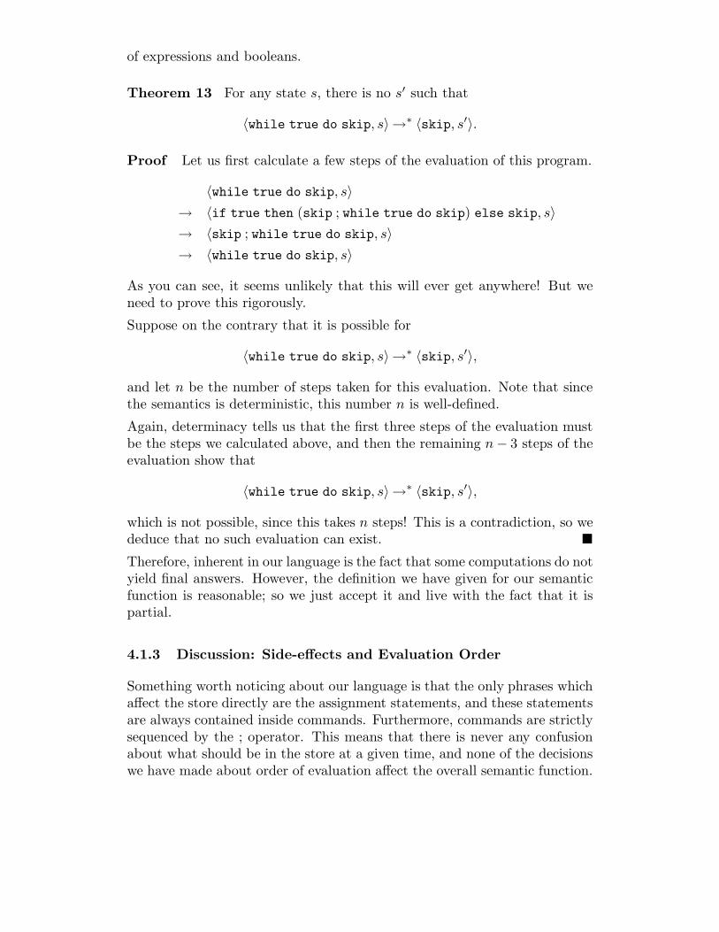
This problem is not particularly severe. It seems likely that a type systemcould be imposed, for example, to prevent programs from attempting toread from variables that have not been initialised. A much more seriousobstruction to the definition of OS [[−]] is the possibility of a nonterminatingcomputation, that is, an infinite loop; see Slide 55.

Let us prove the claim we made, that while true do skip never reaches aresult. Before we do so, let us record a familiar fact about this semantics:determinacy.

Lemma 12 The small-step semantics is deterministic, that is to say, for anyconfiguration 〈P, s〉, there is at most one 〈P ′, s′〉 such that 〈P, s〉→ 〈P ′, s′〉.

Exercise Prove this claim. You should concentrate on the cases of com-mands, and just give an indication of any interesting nuances for the cases

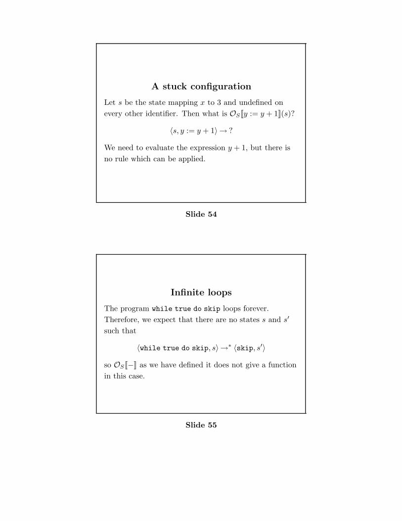
A stuck configuration

Let s be the state mapping x to 3 and undefined on

every other identifier. Then what is OS [[y := y + 1]](s)?

〈s, y := y + 1〉 → ?

We need to evaluate the expression y + 1, but there is

no rule which can be applied.

Slide 54

Infinite loops

The program while true do skip loops forever.

Therefore, we expect that there are no states s and s′

such that

〈while true do skip, s〉→∗ 〈skip, s′〉

so OS [[−]] as we have defined it does not give a function

in this case.

Slide 55

of expressions and booleans.

Theorem 13 For any state s, there is no s′ such that

〈while true do skip, s〉 →∗ 〈skip, s′〉.

Proof Let us first calculate a few steps of the evaluation of this program.

〈while true do skip, s〉

→ 〈if true then (skip ; while true do skip) else skip, s〉

→ 〈skip ; while true do skip, s〉

→ 〈while true do skip, s〉

As you can see, it seems unlikely that this will ever get anywhere! But weneed to prove this rigorously.

Suppose on the contrary that it is possible for

〈while true do skip, s〉 →∗ 〈skip, s′〉,

and let n be the number of steps taken for this evaluation. Note that sincethe semantics is deterministic, this number n is well-defined.

Again, determinacy tells us that the first three steps of the evaluation mustbe the steps we calculated above, and then the remaining n − 3 steps of theevaluation show that

〈while true do skip, s〉 →∗ 〈skip, s′〉,

which is not possible, since this takes n steps! This is a contradiction, so wededuce that no such evaluation can exist. !

Therefore, inherent in our language is the fact that some computations do notyield final answers. However, the definition we have given for our semanticfunction is reasonable; so we just accept it and live with the fact that it ispartial.

4.1.3 Discussion: Side-effects and Evaluation Order

Something worth noticing about our language is that the only phrases whichaffect the store directly are the assignment statements, and these statementsare always contained inside commands. Furthermore, commands are strictlysequenced by the ; operator. This means that there is never any confusionabout what should be in the store at a given time, and none of the decisionswe have made about order of evaluation affect the overall semantic function.

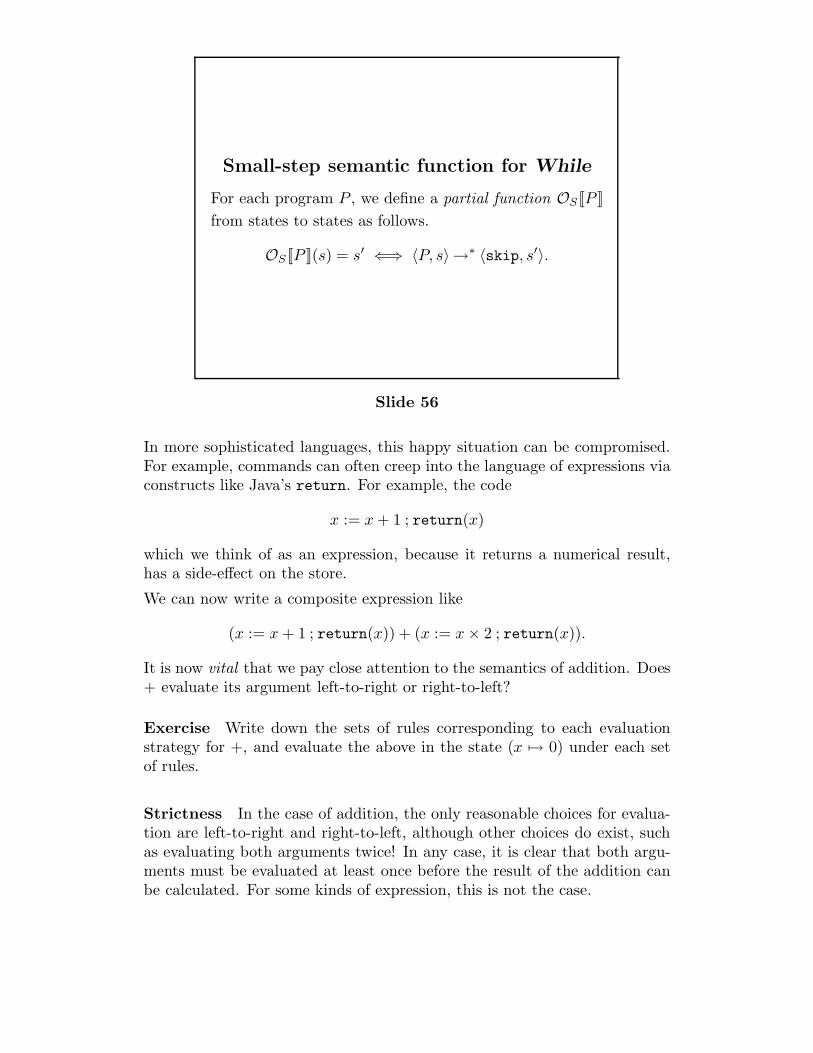
Small-step semantic function for While

For each program P , we define a partial function OS [[P ]]

from states to states as follows.

OS [[P ]](s) = s′ ⇐⇒ 〈P, s〉→∗ 〈skip, s′〉.

Slide 56

In more sophisticated languages, this happy situation can be compromised.For example, commands can often creep into the language of expressions viaconstructs like Java’s return. For example, the code

x := x + 1 ; return(x)

which we think of as an expression, because it returns a numerical result,has a side-effect on the store.

We can now write a composite expression like

(x := x + 1 ; return(x)) + (x := x × 2 ; return(x)).

It is now vital that we pay close attention to the semantics of addition. Does+ evaluate its argument left-to-right or right-to-left?

Exercise Write down the sets of rules corresponding to each evaluationstrategy for +, and evaluate the above in the state (x ,→ 0) under each setof rules.

Strictness In the case of addition, the only reasonable choices for evalua-tion are left-to-right and right-to-left, although other choices do exist, suchas evaluating both arguments twice! In any case, it is clear that both argu-ments must be evaluated at least once before the result of the addition canbe calculated. For some kinds of expression, this is not the case.

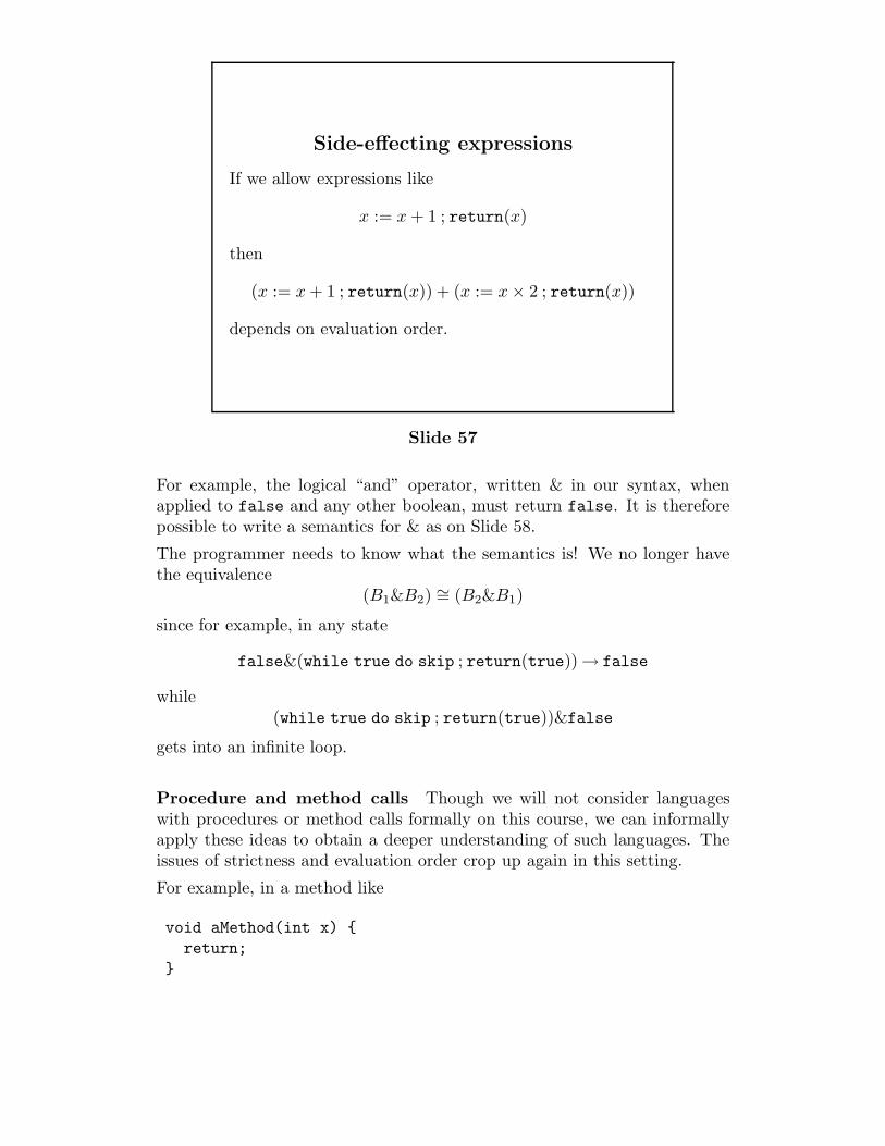
Side-effecting expressions

If we allow expressions like

x := x + 1 ; return(x)

then

(x := x + 1 ; return(x)) + (x := x × 2 ; return(x))

depends on evaluation order.

Slide 57

For example, the logical “and” operator, written & in our syntax, whenapplied to false and any other boolean, must return false. It is thereforepossible to write a semantics for & as on Slide 58.

The programmer needs to know what the semantics is! We no longer havethe equivalence

(B1&B2) ∼= (B2&B1)

since for example, in any state

false&(while true do skip ; return(true)) → false

while(while true do skip ; return(true))&false

gets into an infinite loop.

Procedure and method calls Though we will not consider languageswith procedures or method calls formally on this course, we can informallyapply these ideas to obtain a deeper understanding of such languages. Theissues of strictness and evaluation order crop up again in this setting.

For example, in a method like

void aMethod(int x) {return;

}

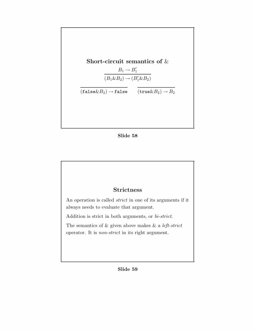
Short-circuit semantics of &

B1 → B′

1

(B1&B2) → (B′

1&B2)

(false&B2) → false (true&B2) → B2

Slide 58

Strictness

An operation is called strict in one of its arguments if it

always needs to evaluate that argument.

Addition is strict in both arguments, or bi-strict.

The semantics of & given above makes & a left-strict

operator. It is non-strict in its right argument.

Slide 59

the argument x is never used. So in a call such as

aMethod(y := y + 1; return y)

do we need to evaluate the argument? Clearly, the outcome of a programcontaining a call like this will depend on the semantic decision we make here.

In a method call such as

anotherMethod(exp1, exp2)

in what order should we evaluate the arguments, if they are used? If anargument is used twice in the body of the method, should it be evaluatedtwice? There are plenty of different semantic decisions to be made here.Some popular choices are:

• evaluate all arguments, left to right, and use the result of this evaluationeach time the argument is used; this is called call-by-value, and isroughly what Java and ML do.

• replace each use of an argument in the method body by the text of theactual parameter the programmer has supplied, so that each time theargument is called, it is re-evaluated. This is call-by-name, and is whatAlgol 60 did (does?).

• evaluate an argument only when it is actually used in the body of themethod, but then remember the result so that if the argument is usedagain, it is not re-evaluated. This is call-by-need, and is what a largenumber of functional languages like Haskell do.

Exercise Write the code of a method myMethod(exp1, exp2) and a par-ticular call of this method, such that the three evaluation strategies aboveall give different results.

The purpose of this discussion is to alert you to the fact that there maybe several reasonable but nonetheless crucially different choices to be madeabout the semantics of various language constructs. One role of a formalstudy of semantics is to help discover where such choices and ambiguities lie,and to resolve them in a fixed, clear and well-documented way.

4.2 Denotational Semantics

We shall now try to give a denotational semantics to the simple language ofwhile-programs. The first step is to choose our semantic domains.

4.2.1 Semantic Domain for Commands

Let us focus first of all on commands, which are the biggest difference betweenWhile and Exp. The small-step operational semantics gave us a partialfunction of the form

OS [[C]](s) = s′

that is, given a command, we have a partial function OS [[C]] from states tostates. This suggests that we might use the set of partial functions fromstates to states, or something like it, as our semantic domain for commands.

Let Σ be the set of all states. Define Σ⊥ to be the set Σ ∪ {⊥}, that is, theset Σ together with an extra element ⊥, called undefined or bottom, whichrepresents a stuck computation or an infinite loop. Then the set of statetransformers is defined on Slide 60.

State Transformers

The set of state transformers is defined to be

ST = [Σ→ Σ⊥]

that is, the set of (total) functions which take a starting

state and return either ⊥, to indicate that the

computation got stuck or looped forever, or a final state.

Slide 60

The set ST will be our semantic domain for commands.

A note on notation The metavariable s, and variants of it like s′ and soon, will be used to range over proper states, not including ⊥. So, if we saythat f(s) = s′, it is implicit that s′ 1= ⊥.

4.2.2 Other Semantic Domains

For booleans and expressions, note that our language allows a boolean oran expression to depend upon the store, but not to change it. Also, though

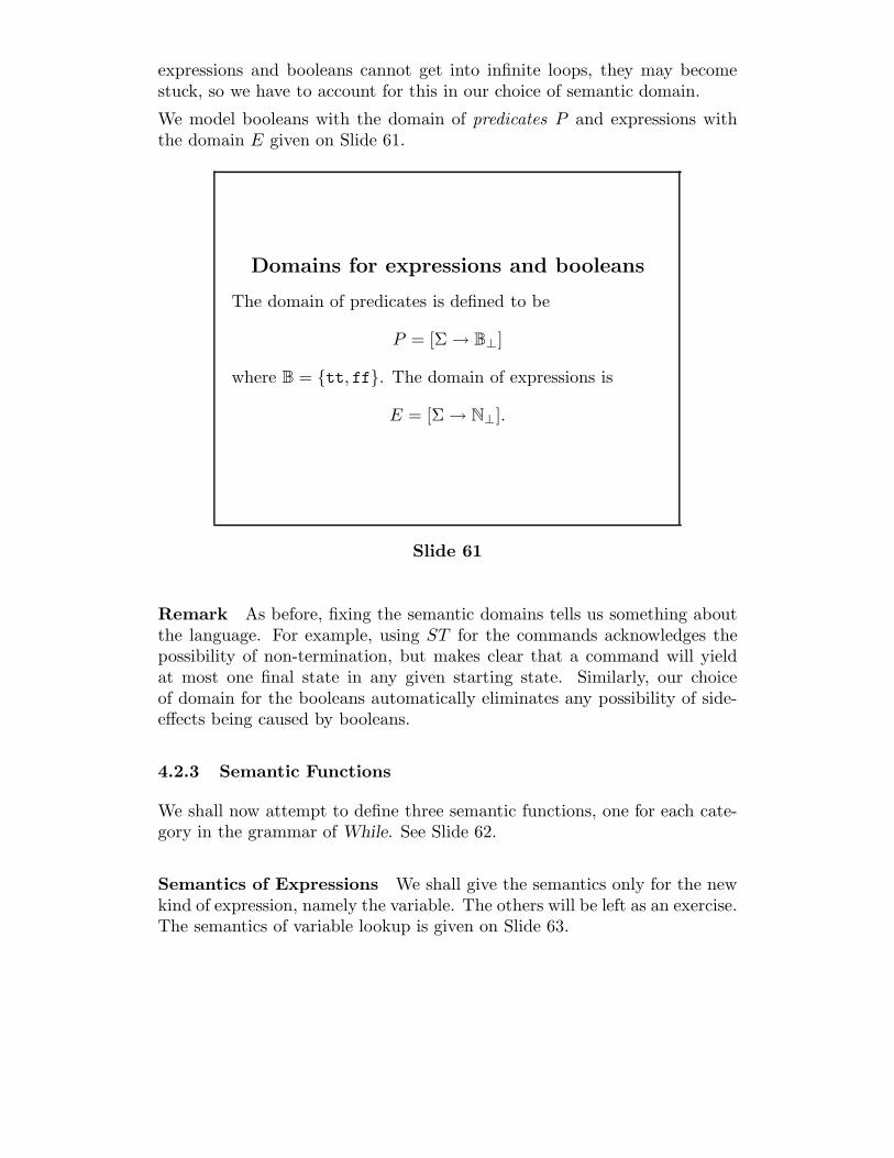
expressions and booleans cannot get into infinite loops, they may becomestuck, so we have to account for this in our choice of semantic domain.

We model booleans with the domain of predicates P and expressions withthe domain E given on Slide 61.

Domains for expressions and booleans

The domain of predicates is defined to be

P = [Σ→ B⊥]

where B = {tt, ff}. The domain of expressions is

E = [Σ→ N⊥].

Slide 61

Remark As before, fixing the semantic domains tells us something aboutthe language. For example, using ST for the commands acknowledges thepossibility of non-termination, but makes clear that a command will yieldat most one final state in any given starting state. Similarly, our choiceof domain for the booleans automatically eliminates any possibility of side-effects being caused by booleans.

4.2.3 Semantic Functions

We shall now attempt to define three semantic functions, one for each cate-gory in the grammar of While. See Slide 62.

Semantics of Expressions We shall give the semantics only for the newkind of expression, namely the variable. The others will be left as an exercise.The semantics of variable lookup is given on Slide 63.

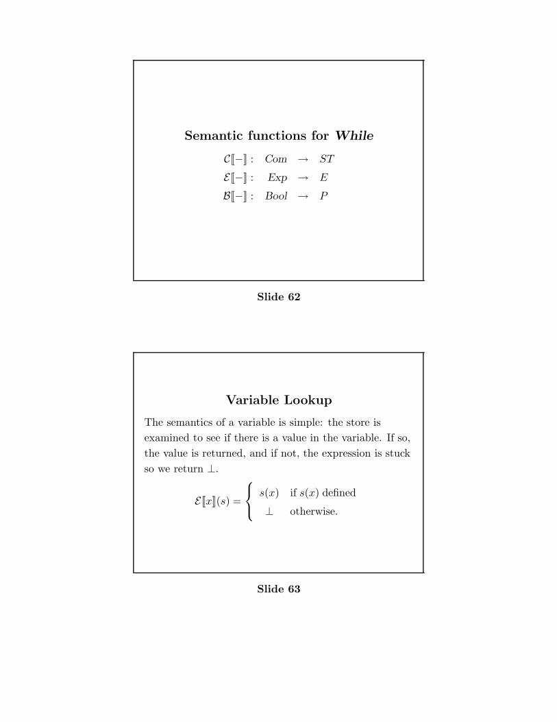
Semantic functions for While

C[[−]] : Com → ST

E [[−]] : Exp → E

B[[−]] : Bool → P

Slide 62

Variable Lookup

The semantics of a variable is simple: the store is

examined to see if there is a value in the variable. If so,

the value is returned, and if not, the expression is stuck

so we return ⊥.

E [[x]](s) =

s(x) if s(x) defined

⊥ otherwise.

Slide 63

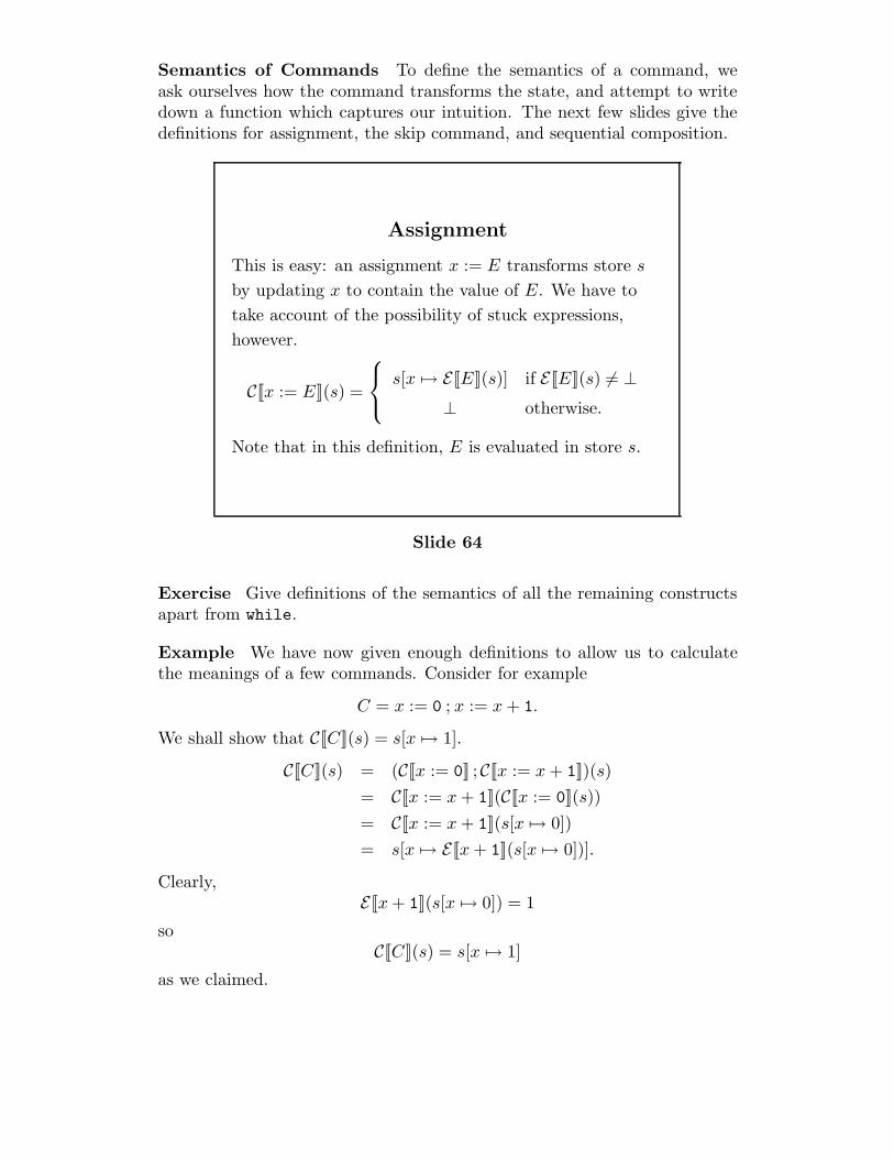
Semantics of Commands To define the semantics of a command, weask ourselves how the command transforms the state, and attempt to writedown a function which captures our intuition. The next few slides give thedefinitions for assignment, the skip command, and sequential composition.

Assignment

This is easy: an assignment x := E transforms store s

by updating x to contain the value of E. We have to

take account of the possibility of stuck expressions,

however.

C[[x := E]](s) =

s[x ,→ E [[E]](s)] if E [[E]](s) 1= ⊥

⊥ otherwise.

Note that in this definition, E is evaluated in store s.

Slide 64

Exercise Give definitions of the semantics of all the remaining constructsapart from while.

Example We have now given enough definitions to allow us to calculatethe meanings of a few commands. Consider for example

C = x := 0 ; x := x + 1.

We shall show that C[[C]](s) = s[x ,→ 1].

C[[C]](s) = (C[[x := 0]] ;C[[x := x + 1]])(s)

= C[[x := x + 1]](C[[x := 0]](s))

= C[[x := x + 1]](s[x ,→ 0])

= s[x ,→ E [[x + 1]](s[x ,→ 0])].

Clearly,E [[x + 1]](s[x ,→ 0]) = 1

soC[[C]](s) = s[x ,→ 1]

as we claimed.

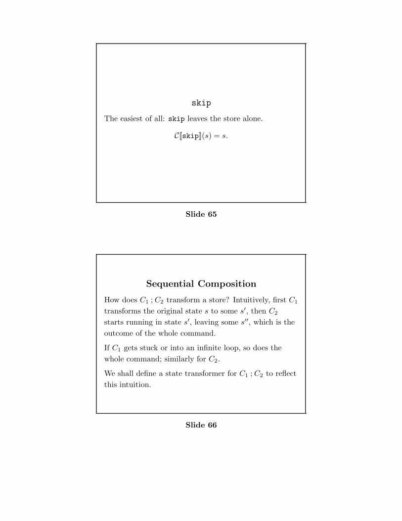
skip

The easiest of all: skip leaves the store alone.

C[[skip]](s) = s.

Slide 65

Sequential Composition

How does C1 ; C2 transform a store? Intuitively, first C1

transforms the original state s to some s′, then C2

starts running in state s′, leaving some s′′, which is the

outcome of the whole command.

If C1 gets stuck or into an infinite loop, so does the

whole command; similarly for C2.

We shall define a state transformer for C1 ; C2 to reflect

this intuition.

Slide 66

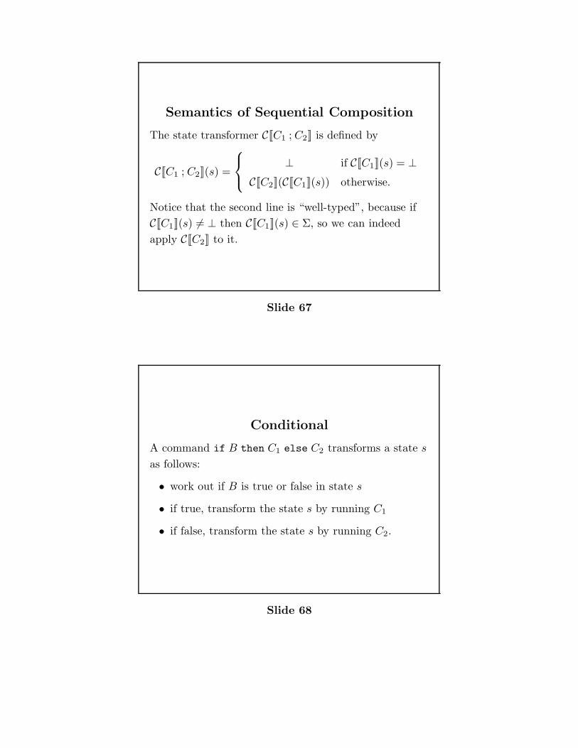
Semantics of Sequential Composition

The state transformer C[[C1 ; C2]] is defined by

C[[C1 ; C2]](s) =

⊥ if C[[C1]](s) = ⊥

C[[C2]](C[[C1]](s)) otherwise.

Notice that the second line is “well-typed”, because if

C[[C1]](s) 1= ⊥ then C[[C1]](s) ∈ Σ, so we can indeed

apply C[[C2]] to it.

Slide 67

Conditional

A command if B then C1 else C2 transforms a state s

as follows:

• work out if B is true or false in state s

• if true, transform the state s by running C1

• if false, transform the state s by running C2.

Slide 68

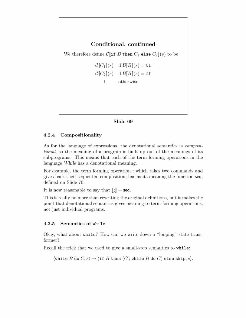
Conditional, continued

We therefore define C[[if B then C1 else C2]](s) to be

C[[C1]](s) if B[[B]](s) = tt

C[[C2]](s) if B[[B]](s) = ff

⊥ otherwise

Slide 69

4.2.4 Compositionality

As for the language of expressions, the denotational semantics is composi-tional, so the meaning of a program is built up out of the meanings of itssubprograms. This means that each of the term forming operations in thelanguage While has a denotational meaning.

For example, the term forming operation ; which takes two commands andgives back their sequential composition, has as its meaning the function seq,defined on Slide 70.

It is now reasonable to say that [[;]] = seq.

This is really no more than rewriting the original definitions, but it makes thepoint that denotational semantics gives meaning to term-forming operations,not just individual programs.

4.2.5 Semantics of while

Okay, what about while? How can we write down a “looping” state trans-former?

Recall the trick that we used to give a small-step semantics to while:

〈while B do C, s〉 → 〈if B then (C ; while B do C) else skip, s〉.

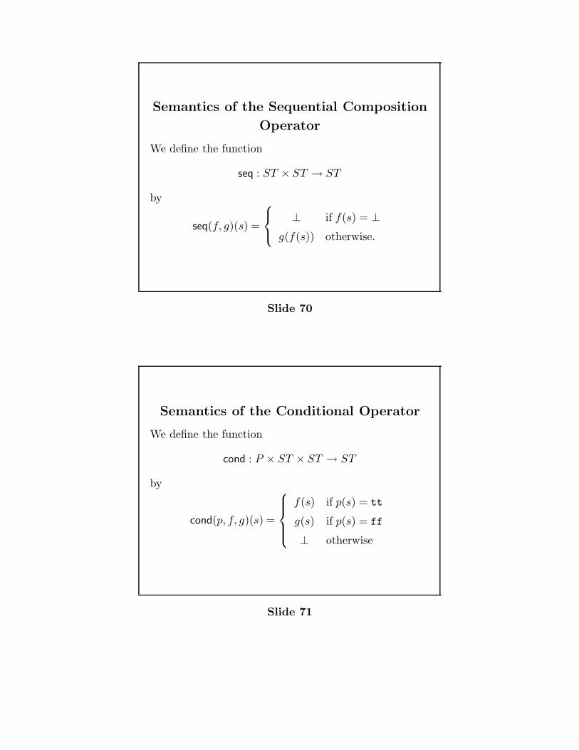
Semantics of the Sequential Composition

Operator

We define the function

seq : ST × ST → ST

by

seq(f, g)(s) =

⊥ if f(s) = ⊥

g(f(s)) otherwise.

Slide 70

Semantics of the Conditional Operator

We define the function

cond : P × ST × ST → ST

by

cond(p, f, g)(s) =

f(s) if p(s) = tt

g(s) if p(s) = ff

⊥ otherwise

Slide 71

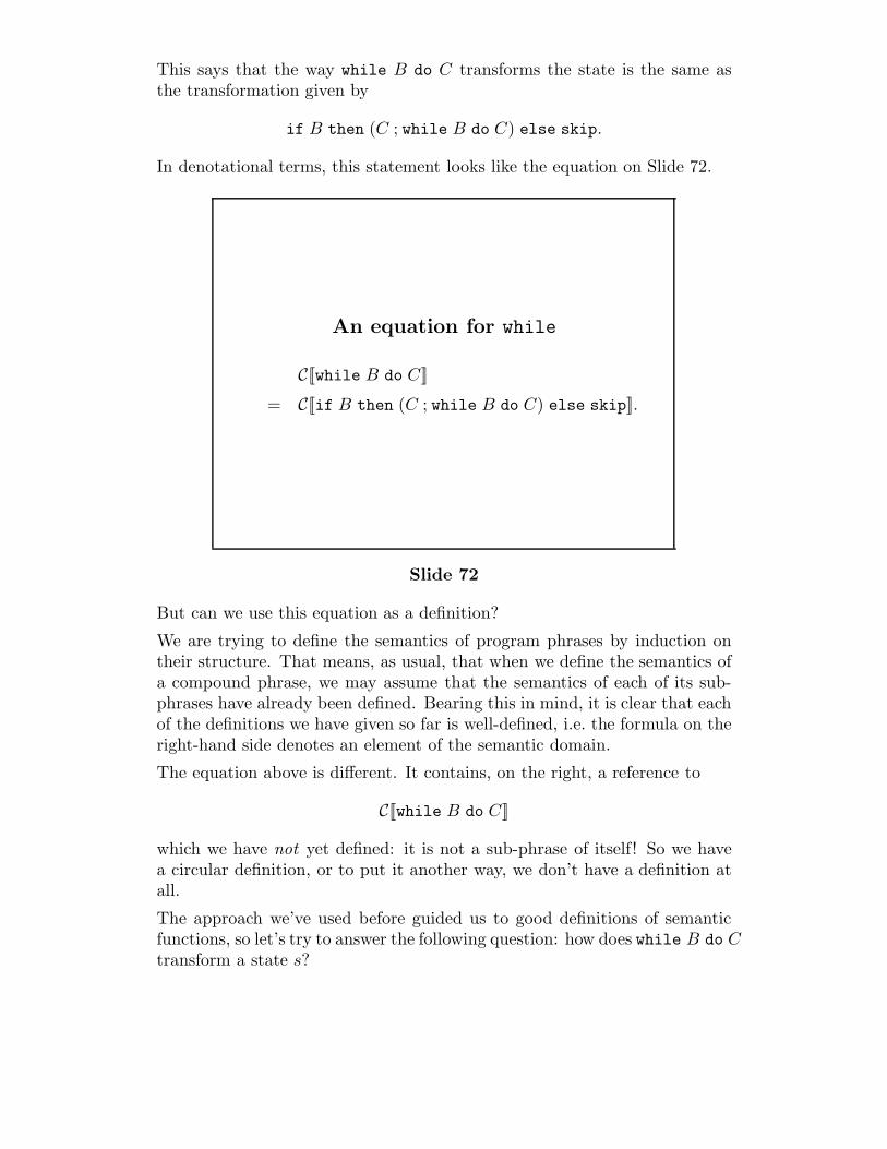
This says that the way while B do C transforms the state is the same asthe transformation given by

if B then (C ; while B do C) else skip.

In denotational terms, this statement looks like the equation on Slide 72.

An equation for while

C[[while B do C]]

= C[[if B then (C ; while B do C) else skip]].

Slide 72

But can we use this equation as a definition?

We are trying to define the semantics of program phrases by induction ontheir structure. That means, as usual, that when we define the semantics ofa compound phrase, we may assume that the semantics of each of its sub-phrases have already been defined. Bearing this in mind, it is clear that eachof the definitions we have given so far is well-defined, i.e. the formula on theright-hand side denotes an element of the semantic domain.

The equation above is different. It contains, on the right, a reference to

C[[while B do C]]

which we have not yet defined: it is not a sub-phrase of itself! So we havea circular definition, or to put it another way, we don’t have a definition atall.

The approach we’ve used before guided us to good definitions of semanticfunctions, so let’s try to answer the following question: how does while B do Ctransform a state s?

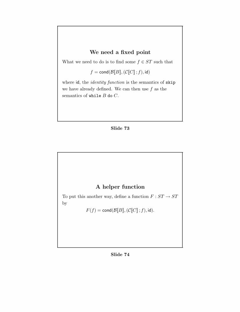
We need a fixed point

What we need to do is to find some f ∈ ST such that

f = cond(B[[B]], (C[[C]] ;f), id)

where id, the identity function is the semantics of skip

we have already defined. We can then use f as the

semantics of while B do C.

Slide 73

A helper function

To put this another way, define a function F : ST → ST

by

F (f) = cond(B[[B]], (C[[C]] ;f), id).

Slide 74

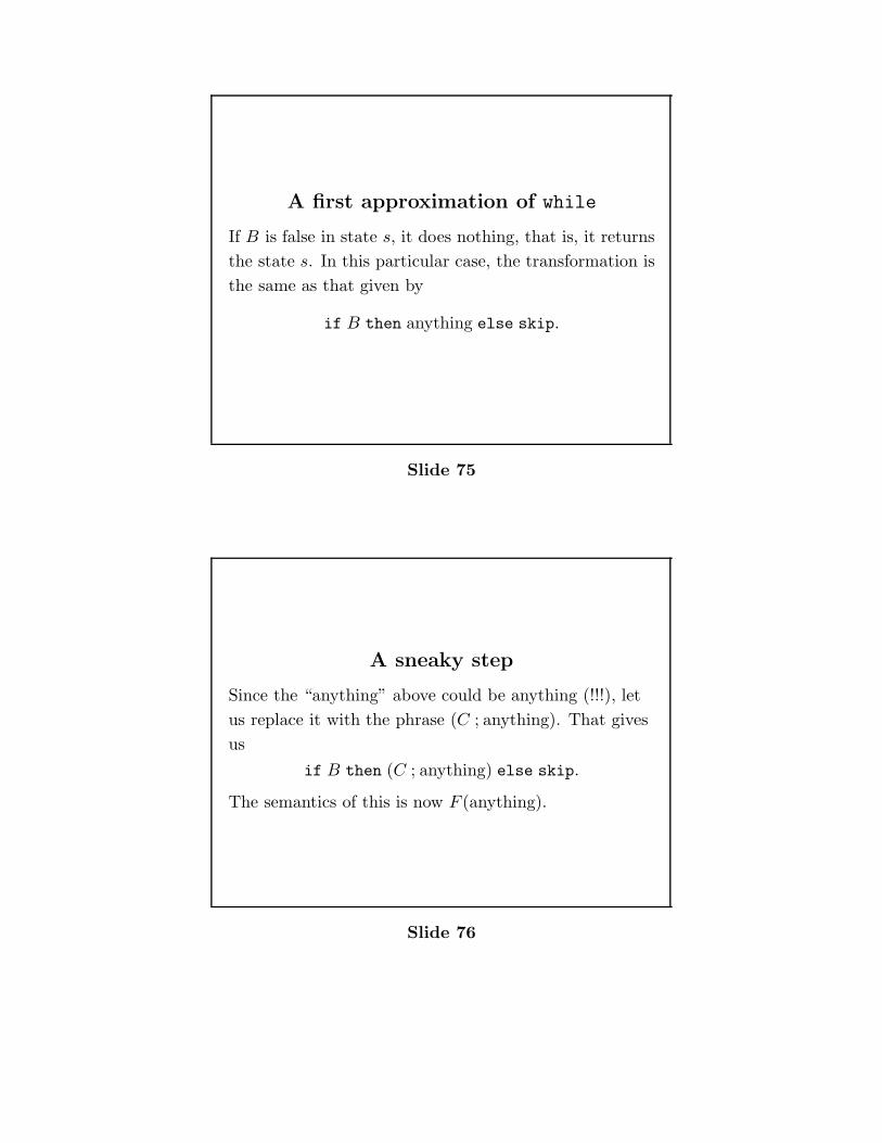
A first approximation of while

If B is false in state s, it does nothing, that is, it returns

the state s. In this particular case, the transformation is

the same as that given by

if B then anything else skip.

Slide 75

A sneaky step

Since the “anything” above could be anything (!!!), let

us replace it with the phrase (C ; anything). That gives

us

if B then (C ; anything) else skip.

The semantics of this is now F (anything).

Slide 76

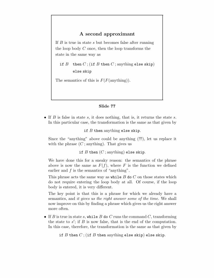
A second approximant

If B is true in state s but becomes false after running

the loop body C once, then the loop transforms the

state in the same way as

if B then C ; (if B then C ; anything else skip)

else skip

The semantics of this is F (F (anything)).

Slide 77

• If B is false in state s, it does nothing, that is, it returns the state s.In this particular case, the transformation is the same as that given by

if B then anything else skip.

Since the “anything” above could be anything (!!!), let us replace itwith the phrase (C ; anything). That gives us

if B then (C ; anything) else skip.

We have done this for a sneaky reason: the semantics of the phraseabove is now the same as F (f), where F is the function we definedearlier and f is the semantics of “anything”.

This phrase acts the same way as while B do C on those states whichdo not require entering the loop body at all. Of course, if the loopbody is entered, it is very different.

The key point is that this is a phrase for which we already have asemantics, and it gives us the right answer some of the time. We shallnow improve on this by finding a phrase which gives us the right answermore often.

• If B is true in state s, while B do C runs the command C, transformingthe state to s′; if B is now false, that is the end of the computation.In this case, therefore, the transformation is the same as that given by

if B then C ; (if B then anything else skip) else skip.

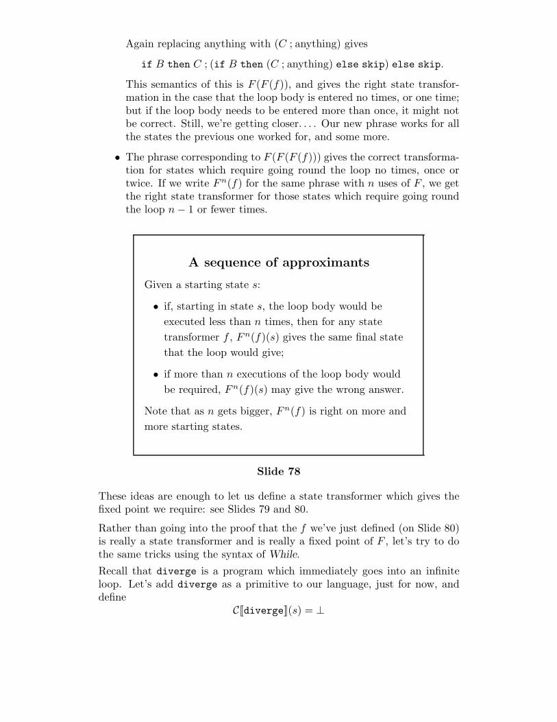
Again replacing anything with (C ; anything) gives

if B then C ; (if B then (C ; anything) else skip) else skip.

This semantics of this is F (F (f)), and gives the right state transfor-mation in the case that the loop body is entered no times, or one time;but if the loop body needs to be entered more than once, it might notbe correct. Still, we’re getting closer. . . . Our new phrase works for allthe states the previous one worked for, and some more.

• The phrase corresponding to F (F (F (f))) gives the correct transforma-tion for states which require going round the loop no times, once ortwice. If we write Fn(f) for the same phrase with n uses of F , we getthe right state transformer for those states which require going roundthe loop n − 1 or fewer times.

A sequence of approximants

Given a starting state s:

• if, starting in state s, the loop body would be

executed less than n times, then for any state

transformer f , Fn(f)(s) gives the same final state

that the loop would give;

• if more than n executions of the loop body would

be required, Fn(f)(s) may give the wrong answer.

Note that as n gets bigger, Fn(f) is right on more and

more starting states.

Slide 78

These ideas are enough to let us define a state transformer which gives thefixed point we require: see Slides 79 and 80.

Rather than going into the proof that the f we’ve just defined (on Slide 80)is really a state transformer and is really a fixed point of F , let’s try to dothe same tricks using the syntax of While.

Recall that diverge is a program which immediately goes into an infiniteloop. Let’s add diverge as a primitive to our language, just for now, anddefine

C[[diverge]](s) = ⊥

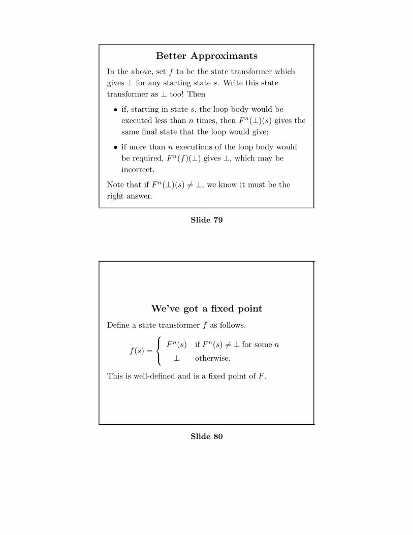
Better Approximants

In the above, set f to be the state transformer which

gives ⊥ for any starting state s. Write this state

transformer as ⊥ too! Then

• if, starting in state s, the loop body would be

executed less than n times, then Fn(⊥)(s) gives the

same final state that the loop would give;

• if more than n executions of the loop body would

be required, Fn(f)(⊥) gives ⊥, which may be

incorrect.

Note that if Fn(⊥)(s) 1= ⊥, we know it must be the

right answer.

Slide 79

We’ve got a fixed point

Define a state transformer f as follows.

f(s) =

Fn(s) if Fn(s) 1= ⊥ for some n

⊥ otherwise.

This is well-defined and is a fixed point of F .

Slide 80

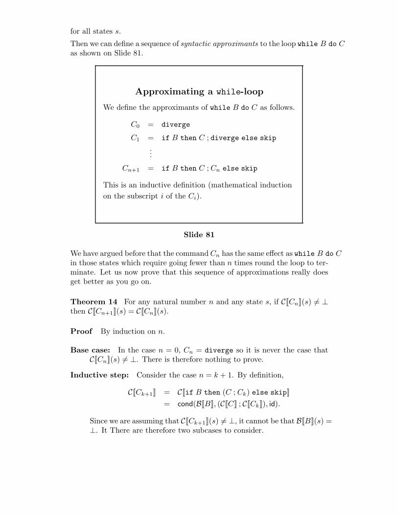
for all states s.

Then we can define a sequence of syntactic approximants to the loop while B do Cas shown on Slide 81.

Approximating a while-loop

We define the approximants of while B do C as follows.

C0 = diverge

C1 = if B then C ; diverge else skip

...

Cn+1 = if B then C ; Cn else skip

This is an inductive definition (mathematical induction

on the subscript i of the Ci).

Slide 81

We have argued before that the command Cn has the same effect as while B do Cin those states which require going fewer than n times round the loop to ter-minate. Let us now prove that this sequence of approximations really doesget better as you go on.

Theorem 14 For any natural number n and any state s, if C[[Cn]](s) 1= ⊥then C[[Cn+1]](s) = C[[Cn]](s).

Proof By induction on n.

Base case: In the case n = 0, Cn = diverge so it is never the case thatC[[Cn]](s) 1= ⊥. There is therefore nothing to prove.

Inductive step: Consider the case n = k + 1. By definition,

C[[Ck+1]] = C[[if B then (C ; Ck) else skip]]

= cond(B[[B]], (C[[C]] ; C[[Ck]]), id).

Since we are assuming that C[[Ck+1]](s) 1= ⊥, it cannot be that B[[B]](s) =⊥. It There are therefore two subcases to consider.

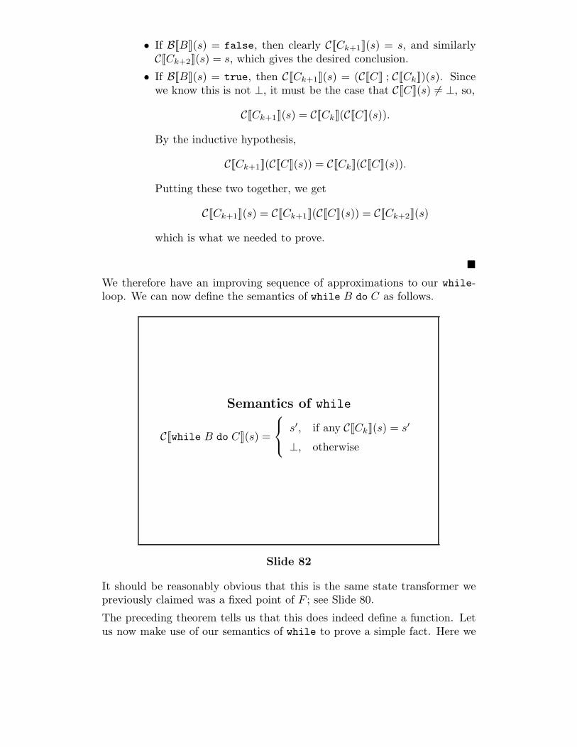
• If B[[B]](s) = false, then clearly C[[Ck+1]](s) = s, and similarlyC[[Ck+2]](s) = s, which gives the desired conclusion.

• If B[[B]](s) = true, then C[[Ck+1]](s) = (C[[C]] ; C[[Ck]])(s). Sincewe know this is not ⊥, it must be the case that C[[C]](s) 1= ⊥, so,

C[[Ck+1]](s) = C[[Ck]](C[[C]](s)).

By the inductive hypothesis,

C[[Ck+1]](C[[C]](s)) = C[[Ck]](C[[C]](s)).

Putting these two together, we get

C[[Ck+1]](s) = C[[Ck+1]](C[[C]](s)) = C[[Ck+2]](s)

which is what we needed to prove.

!

We therefore have an improving sequence of approximations to our while-loop. We can now define the semantics of while B do C as follows.

Semantics of while

C[[while B do C]](s) =

s′, if any C[[Ck]](s) = s′

⊥, otherwise

Slide 82

It should be reasonably obvious that this is the same state transformer wepreviously claimed was a fixed point of F ; see Slide 80.

The preceding theorem tells us that this does indeed define a function. Letus now make use of our semantics of while to prove a simple fact. Here we

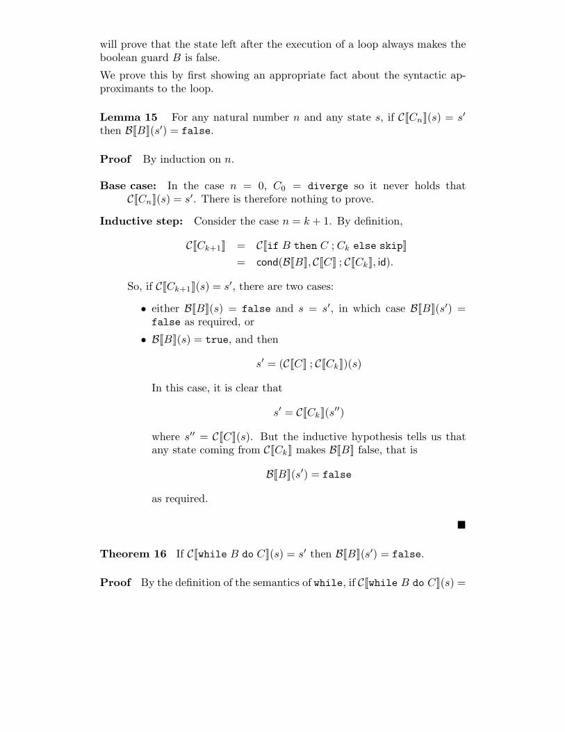
will prove that the state left after the execution of a loop always makes theboolean guard B is false.

We prove this by first showing an appropriate fact about the syntactic ap-proximants to the loop.

Lemma 15 For any natural number n and any state s, if C[[Cn]](s) = s′

then B[[B]](s′) = false.

Proof By induction on n.

Base case: In the case n = 0, C0 = diverge so it never holds thatC[[Cn]](s) = s′. There is therefore nothing to prove.

Inductive step: Consider the case n = k + 1. By definition,

C[[Ck+1]] = C[[if B then C ; Ck else skip]]

= cond(B[[B]], C[[C]] ; C[[Ck]], id).

So, if C[[Ck+1]](s) = s′, there are two cases:

• either B[[B]](s) = false and s = s′, in which case B[[B]](s′) =false as required, or

• B[[B]](s) = true, and then

s′ = (C[[C]] ; C[[Ck]])(s)

In this case, it is clear that

s′ = C[[Ck]](s′′)

where s′′ = C[[C]](s). But the inductive hypothesis tells us thatany state coming from C[[Ck]] makes B[[B]] false, that is

B[[B]](s′) = false

as required.

!

Theorem 16 If C[[while B do C]](s) = s′ then B[[B]](s′) = false.

Proof By the definition of the semantics of while, if C[[while B do C]](s) =

s′ then s′ = C[[Cn]](s) for some n. By the previous lemma, B[[B]](s′) = falseas required. !

Exercise Prove that

• C[[x := y ; y := x]] = C[[x := y]].

• C[[x := z ; y := z]] = C[[y := z ; x := z]].

• C[[C1 ; (C2 ; C3)]] = C[[(C1 ; C2) ; C3]].

Is it the case that C[[x := x]] = C[[skip]] in this language? If so, give a proof;if not, give a counterexample.

4.3 Axiomatic Semantics

We have so far seen two distinct approaches to semantics.

operational: explains how to evaluate programs.

denotational: gives meaning to a program by identifying an element of amathematical structure which “is” the program’s meaning.

Using either of these styles of semantics we can prove various facts aboutprograms, verify correctness of programs with respect to their specification,and so on. We have seen a few examples of this.

The final form of semantics that we shall consider is aimed directly at sup-porting such reasoning and verification.

axiomatic: gives a proof system for verifying program properties.

The axiomatic semantics we shall study is called Hoare logic, after its inven-tor, Tony Hoare. It is sometimes called Floyd-Hoare logic in recognition ofan earlier contribution by Floyd.

4.3.1 Partial Correctness

Hoare logic is a system for demonstrating that certain partial correctnessassertions hold of programs. A partial correctness assertion takes the formshown on Slide 83.

This is called a partial correctness assertion because it says nothing aboutwhat happens if C fails to terminate, and it says nothing about whether Cterminates or not.

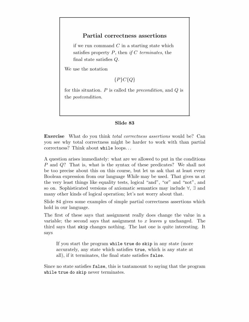
Partial correctness assertions

if we run command C in a starting state which

satisfies property P , then if C terminates, the

final state satisfies Q.

We use the notation

{P}C{Q}

for this situation. P is called the precondition, and Q is

the postcondition.

Slide 83

Exercise What do you think total correctness assertions would be? Canyou see why total correctness might be harder to work with than partialcorrectness? Think about while loops. . .

A question arises immediately: what are we allowed to put in the conditionsP and Q? That is, what is the syntax of these predicates? We shall notbe too precise about this on this course, but let us ask that at least everyBoolean expression from our language While may be used. That gives us atthe very least things like equality tests, logical “and”, “or” and “not”, andso on. Sophisticated versions of axiomatic semantics may include ∀, ∃ andmany other kinds of logical operation; let’s not worry about that.

Slide 84 gives some examples of simple partial correctness assertions whichhold in our language.

The first of these says that assignment really does change the value in avariable; the second says that assignment to x leaves y unchanged. Thethird says that skip changes nothing. The last one is quite interesting. Itsays

If you start the program while true do skip in any state (moreaccurately, any state which satisfies true, which is any state atall), if it terminates, the final state satisfies false.

Since no state satisfies false, this is tantamount to saying that the programwhile true do skip never terminates.

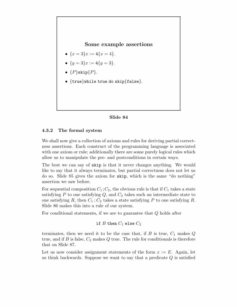
Some example assertions

• {x = 3}x := 4{x = 4}.

• {y = 3}x := 4{y = 3}.

• {P}skip{P}.

• {true}while true do skip{false}.

Slide 84

4.3.2 The formal system

We shall now give a collection of axioms and rules for deriving partial correct-ness assertions. Each construct of the programming language is associatedwith one axiom or rule; additionally there are some purely logical rules whichallow us to manipulate the pre- and postconditions in certain ways.

The best we can say of skip is that it never changes anything. We wouldlike to say that it always terminates, but partial correctness does not let usdo so. Slide 85 gives the axiom for skip, which is the same “do nothing”assertion we saw before.

For sequential composition C1 ;C2, the obvious rule is that if C1 takes a statesatisfying P to one satisfying Q, and C2 takes such an intermediate state toone satisfying R, then C1 ; C2 takes a state satisfying P to one satisfying R.Slide 86 makes this into a rule of our system.

For conditional statements, if we are to guarantee that Q holds after

if B then C1 else C2

terminates, then we need it to be the case that, if B is true, C1 makes Qtrue, and if B is false, C2 makes Q true. The rule for conditionals is thereforethat on Slide 87.

Let us now consider assignment statements of the form x := E. Again, letus think backwards. Suppose we want to say that a predicate Q is satisfied

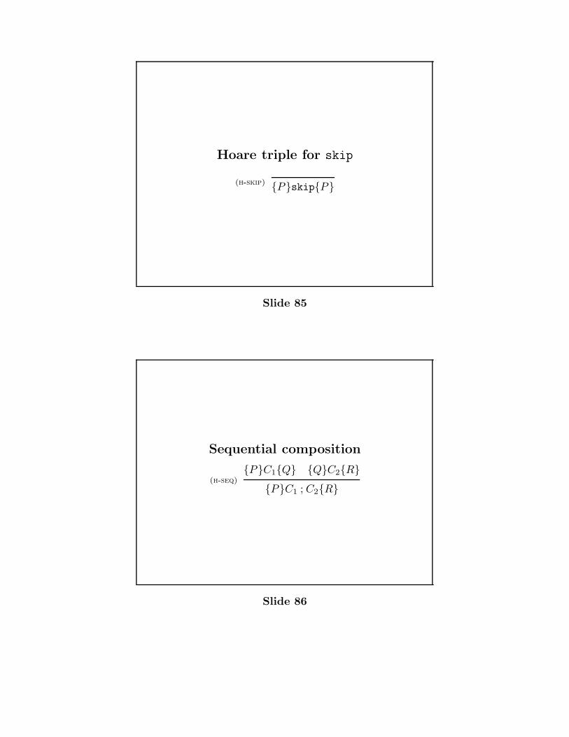
Hoare triple for skip

(h-skip) {P}skip{P}

Slide 85

Sequential composition

(h-seq){P}C1{Q} {Q}C2{R}

{P}C1 ; C2{R}

Slide 86

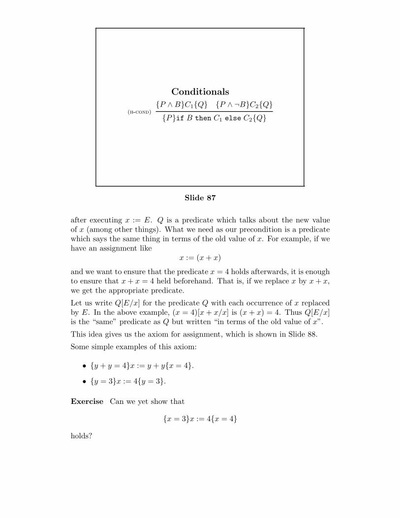
Conditionals

(h-cond){P ∧ B}C1{Q} {P ∧ ¬B}C2{Q}

{P}if B then C1 else C2{Q}

Slide 87

after executing x := E. Q is a predicate which talks about the new valueof x (among other things). What we need as our precondition is a predicatewhich says the same thing in terms of the old value of x. For example, if wehave an assignment like

x := (x + x)

and we want to ensure that the predicate x = 4 holds afterwards, it is enoughto ensure that x + x = 4 held beforehand. That is, if we replace x by x + x,we get the appropriate predicate.

Let us write Q[E/x] for the predicate Q with each occurrence of x replacedby E. In the above example, (x = 4)[x + x/x] is (x + x) = 4. Thus Q[E/x]is the “same” predicate as Q but written “in terms of the old value of x”.

This idea gives us the axiom for assignment, which is shown in Slide 88.

Some simple examples of this axiom:

• {y + y = 4}x := y + y{x = 4}.

• {y = 3}x := 4{y = 3}.

Exercise Can we yet show that

{x = 3}x := 4{x = 4}

holds?

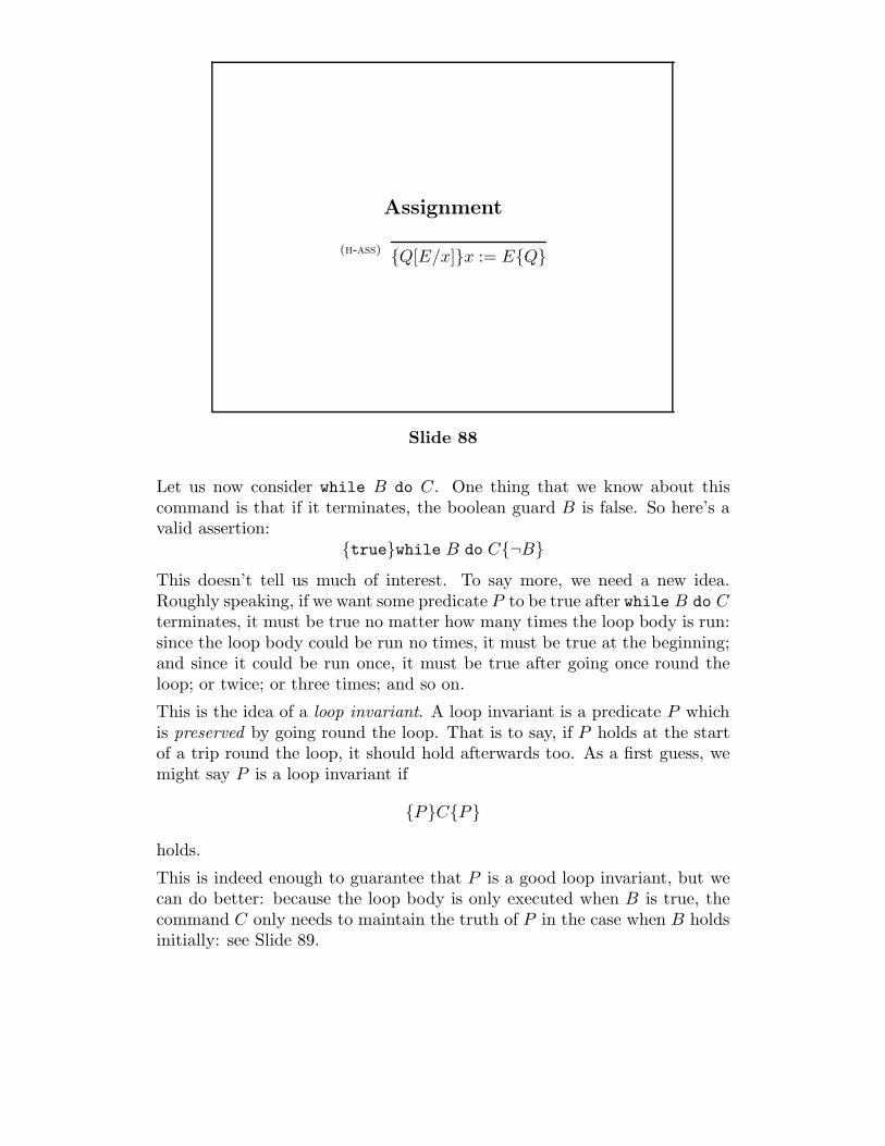
Assignment

(h-ass) {Q[E/x]}x := E{Q}

Slide 88

Let us now consider while B do C. One thing that we know about thiscommand is that if it terminates, the boolean guard B is false. So here’s avalid assertion:

{true}while B do C{¬B}

This doesn’t tell us much of interest. To say more, we need a new idea.Roughly speaking, if we want some predicate P to be true after while B do Cterminates, it must be true no matter how many times the loop body is run:since the loop body could be run no times, it must be true at the beginning;and since it could be run once, it must be true after going once round theloop; or twice; or three times; and so on.

This is the idea of a loop invariant. A loop invariant is a predicate P whichis preserved by going round the loop. That is to say, if P holds at the startof a trip round the loop, it should hold afterwards too. As a first guess, wemight say P is a loop invariant if

{P}C{P}

holds.

This is indeed enough to guarantee that P is a good loop invariant, but wecan do better: because the loop body is only executed when B is true, thecommand C only needs to maintain the truth of P in the case when B holdsinitially: see Slide 89.

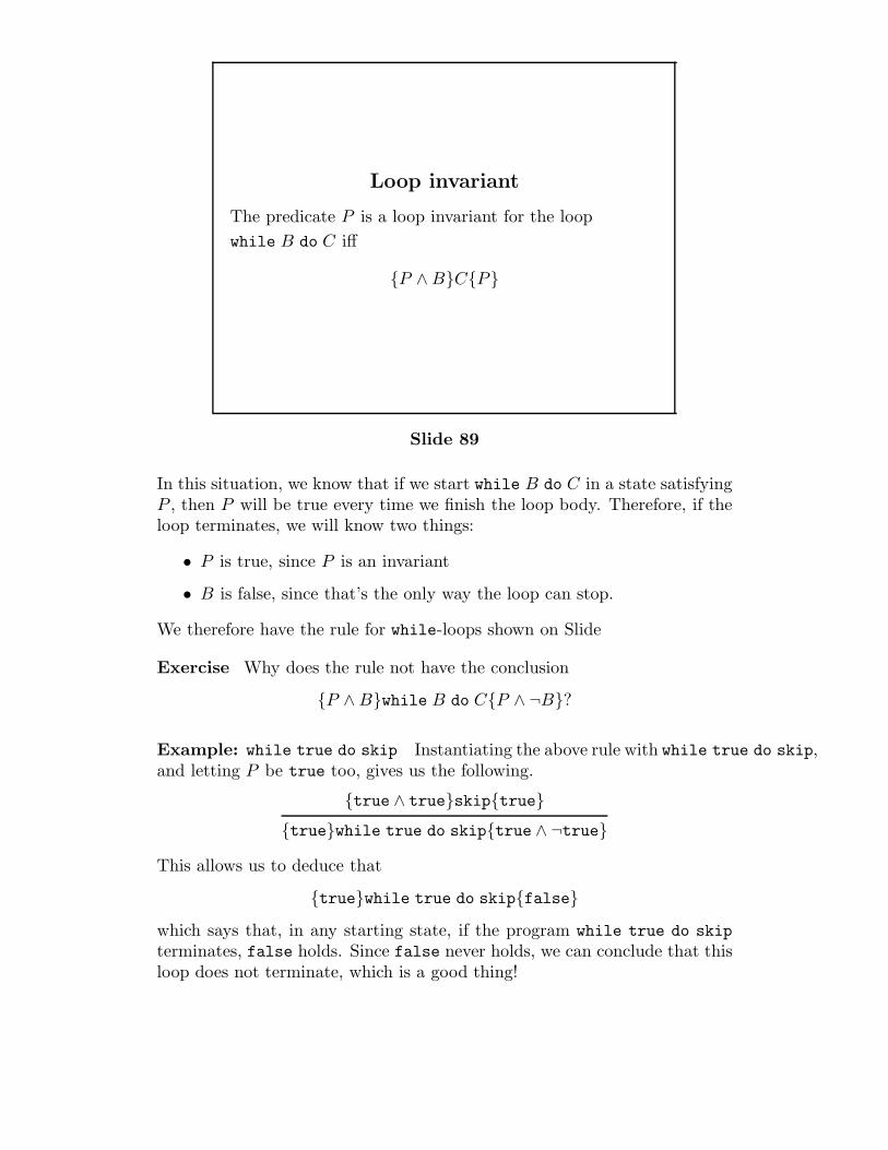
Loop invariant

The predicate P is a loop invariant for the loop

while B do C iff

{P ∧ B}C{P}

Slide 89

In this situation, we know that if we start while B do C in a state satisfyingP , then P will be true every time we finish the loop body. Therefore, if theloop terminates, we will know two things:

• P is true, since P is an invariant

• B is false, since that’s the only way the loop can stop.

We therefore have the rule for while-loops shown on Slide

Exercise Why does the rule not have the conclusion

{P ∧ B}while B do C{P ∧ ¬B}?

Example: while true do skip Instantiating the above rule with while true do skip,and letting P be true too, gives us the following.

{true ∧ true}skip{true}

{true}while true do skip{true ∧ ¬true}

This allows us to deduce that

{true}while true do skip{false}

which says that, in any starting state, if the program while true do skipterminates, false holds. Since false never holds, we can conclude that thisloop does not terminate, which is a good thing!

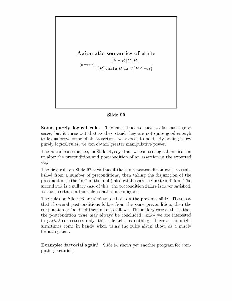
Axiomatic semantics of while

(h-while){P ∧ B}C{P}

{P}while B do C{P ∧ ¬B}

Slide 90

Some purely logical rules The rules that we have so far make goodsense, but it turns out that as they stand they are not quite good enoughto let us prove some of the assertions we expect to hold. By adding a fewpurely logical rules, we can obtain greater manipulative power.

The rule of consequence, on Slide 91, says that we can use logical implicationto alter the precondition and postcondition of an assertion in the expectedway.

The first rule on Slide 92 says that if the same postcondition can be estab-lished from a number of preconditions, then taking the disjunction of thepreconditions (the “or” of them all) also establishes the postcondition. Thesecond rule is a nullary case of this: the precondition false is never satisfied,so the assertion in this rule is rather meaningless.

The rules on Slide 93 are similar to those on the previous slide. These saythat if several postconditions follow from the same precondition, then theconjunction or “and” of them all also follows. The nullary case of this is thatthe postcondition true may always be concluded: since we are interestedin partial correctness only, this rule tells us nothing. However, it mightsometimes come in handy when using the rules given above as a purelyformal system.

Example: factorial again! Slide 94 shows yet another program for com-puting factorials.

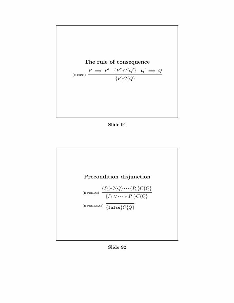
The rule of consequence

(h-cons)P =⇒ P ′ {P ′}C{Q′} Q′ =⇒ Q

{P}C{Q}

Slide 91

Precondition disjunction

(h-pre.or){P1}C{Q} · · · {Pn}C{Q}

{P1 ∨ · · · ∨ Pn}C{Q}

(h-pre.false) {false}C{Q}

Slide 92

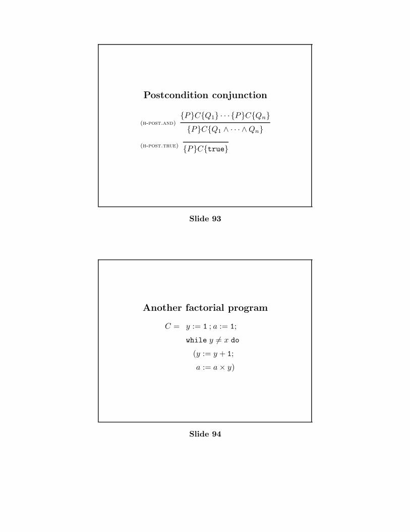
Postcondition conjunction

(h-post.and){P}C{Q1} · · · {P}C{Qn}

{P}C{Q1 ∧ · · · ∧ Qn}

(h-post.true) {P}C{true}

Slide 93

Another factorial program

C = y := 1 ; a := 1;

while y 1= x do

(y := y + 1;

a := a × y)

Slide 94

We are going to show, using the rules given above (but leaving out some ofthe details), that this program computes the value of x!, leaving the resultin the variable a.

The partial correctness assertion we want to establish is

{true}C{a = x!}.

The interesting part here is the loop invariant. The idea of the loop is that aholds a “running product” of all the numbers between 1 and y, so that wheny reaches x, a holds x!.

We might therefore guess that the loop invariant should be

a = 1 × · · ·× y.

Therefore our first task is to show that

{(a = 1 × · · ·× y) ∧ (y 1= x)}y := y + 1 ; a := a × y{a = 1 × · · ·× y}

is a valid assertion. Let us call the precondition above P , and the postcon-dition Q.

We shall show this assertion is valid by applying the rules for assignmentand sequential composition. The assignment rule works right-to-left, so wework backwards through the assignments as shown on Slide 95.

Working backwards through assignments

The assertion

{a × y = 1 × · · ·× y}a := a × y{a = 1 × · · ·× y}

is an instance of the axiom for assignments: the

precondition has been calculated by substituting a × y

for a in the postcondition.

Similarly we can obtain

{a×(y+1) = 1×· · ·×(y+1)}y := y+1{a×y = 1×· · ·×y}

Slide 95

Notice that in doing this calculation, we work from right to left: startingfrom the postcondition we need to establish, we calculate a precondition for

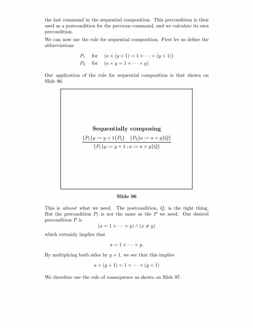
the last command in the sequential composition. This precondition is thenused as a postcondition for the previous command, and we calculate its ownprecondition.

We can now use the rule for sequential composition. First let us define theabbreviations

P1 for (a × (y + 1) = 1 × · · ·× (y + 1))

P2 for (a × y = 1 × · · ·× y)

Our application of the rule for sequential composition is that shown onSlide 96.

Sequentially composing

{P1}y := y + 1{P2} {P2}a := a × y{Q}

{P1}y := y + 1 ; a := a × y{Q}

Slide 96

This is almost what we need. The postcondition, Q, is the right thing.But the precondition P1 is not the same as the P we need. Our desiredprecondition P is

(a = 1 × · · ·× y) ∧ (x 1= y)

which certainly implies that

a = 1 × · · ·× y.

By multiplying both sides by y + 1, we see that this implies

a × (y + 1) = 1 × · · ·× (y + 1)

We therefore use the rule of consequence as shown on Slide 97.

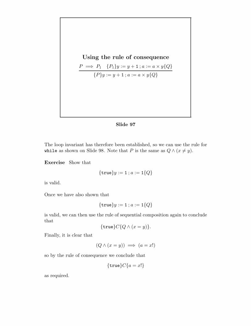
Using the rule of consequence

P =⇒ P1 {P1}y := y + 1 ; a := a × y{Q}

{P}y := y + 1 ; a := a × y{Q}

Slide 97

The loop invariant has therefore been established, so we can use the rule forwhile as shown on Slide 98. Note that P is the same as Q ∧ (x 1= y).

Exercise Show that

{true}y := 1 ; a := 1{Q}

is valid.

Once we have also shown that

{true}y := 1 ; a := 1{Q}

is valid, we can then use the rule of sequential composition again to concludethat

{true}C{Q ∧ (x = y)}.

Finally, it is clear that

(Q ∧ (x = y)) =⇒ (a = x!)

so by the rule of consequence we conclude that

{true}C{a = x!}

as required.

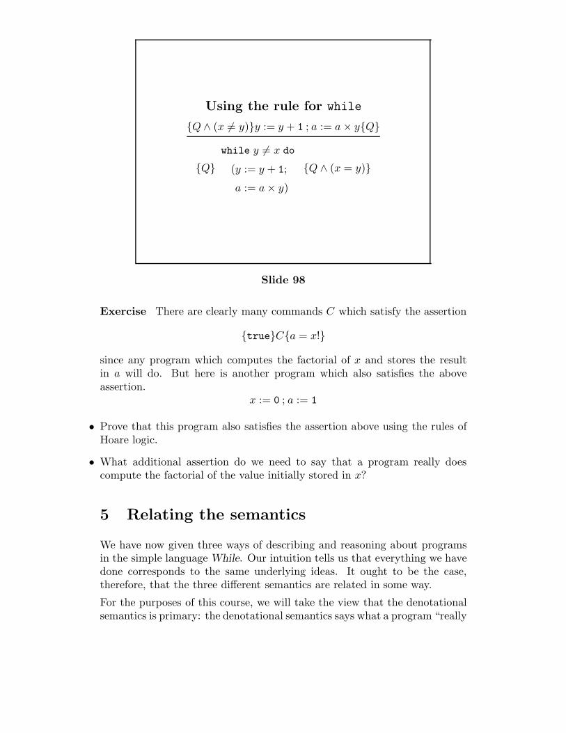
Using the rule for while

{Q ∧ (x 1= y)}y := y + 1 ; a := a × y{Q}

{Q}

while y 1= x do

(y := y + 1;

a := a × y)

{Q ∧ (x = y)}

Slide 98

Exercise There are clearly many commands C which satisfy the assertion

{true}C{a = x!}

since any program which computes the factorial of x and stores the resultin a will do. But here is another program which also satisfies the aboveassertion.

x := 0 ; a := 1

• Prove that this program also satisfies the assertion above using the rules ofHoare logic.

• What additional assertion do we need to say that a program really doescompute the factorial of the value initially stored in x?

5 Relating the semantics

We have now given three ways of describing and reasoning about programsin the simple language While. Our intuition tells us that everything we havedone corresponds to the same underlying ideas. It ought to be the case,therefore, that the three different semantics are related in some way.

For the purposes of this course, we will take the view that the denotationalsemantics is primary: the denotational semantics says what a program “really

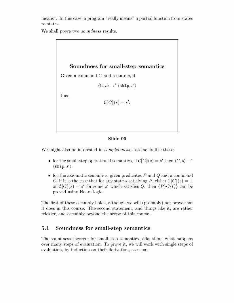
means”. In this case, a program “really means” a partial function from statesto states.

We shall prove two soundness results.

Soundness for small-step semantics

Given a command C and a state s, if

〈C, s〉→∗ 〈skip, s′〉

then

C[[C]](s) = s′.

Slide 99

We might also be interested in completeness statements like these:

• for the small-step operational semantics, if C[[C]](s) = s′ then 〈C, s〉→∗

〈skip, s′〉.

• for the axiomatic semantics, given predicates P and Q and a commandC, if it is the case that for any state s satisfying P , either C[[C]](s) = ⊥or C[[C]](s) = s′ for some s′ which satisfies Q, then {P}C{Q} can beproved using Hoare logic.

The first of these certainly holds, although we will (probably) not prove thatit does in this course. The second statement, and things like it, are rathertrickier, and certainly beyond the scope of this course.

5.1 Soundness for small-step semantics

The soundness theorem for small-step semantics talks about what happensover many steps of evaluation. To prove it, we will work with single steps ofevaluation, by induction on their derivation, as usual.

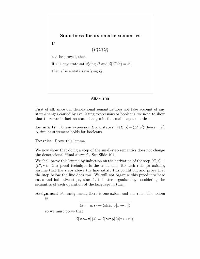
Soundness for axiomatic semantics

If

{P}C{Q}

can be proved, then

if s is any state satisfying P and C[[C]](s) = s′,

then s′ is a state satisfying Q.

Slide 100

First of all, since our denotational semantics does not take account of anystate-changes caused by evaluating expressions or booleans, we need to showthat there are in fact no state changes in the small-step semantics.

Lemma 17 For any expression E and state s, if 〈E, s〉→〈E′, s′〉 then s = s′.A similar statement holds for booleans.

Exercise Prove this lemma.

We now show that doing a step of the small-step semantics does not changethe denotational “final answer”. See Slide 101.

We shall prove this lemma by induction on the derivation of the step 〈C, s〉→〈C′, s′〉. Our proof technique is the usual one: for each rule (or axiom),assume that the steps above the line satisfy this condition, and prove thatthe step below the line does too. We will not organise this proof into basecases and inductive steps, since it is better organised by considering thesemantics of each operation of the language in turn.

Assignment For assignment, there is one axiom and one rule. The axiomis

〈x := n, s〉 → 〈skip, s[x ,→ n]〉

so we must prove that

C[[x := n]](s) = C[[skip]](s[x ,→ n]).

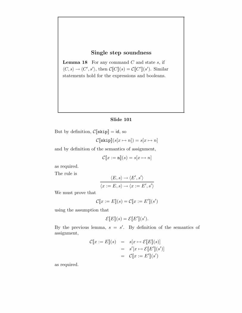
Single step soundness

Lemma 18 For any command C and state s, if

〈C, s〉 → 〈C′, s′〉, then C[[C]](s) = C[[C′]](s′). Similar

statements hold for the expressions and booleans.

Slide 101

But by definition, C[[skip]] = id, so

C[[skip]](s[x ,→ n]) = s[x ,→ n]

and by definition of the semantics of assignment,

C[[x := n]](s) = s[x ,→ n]

as required.

The rule is〈E, s〉→ 〈E′, s′〉

〈x := E, s〉→ 〈x := E′, s′〉

We must prove that

C[[x := E]](s) = C[[x := E′]](s′)

using the assumption that

E [[E]](s) = E [[E′]](s′).

By the previous lemma, s = s′. By definition of the semantics ofassignment,

C[[x := E]](s) = s[x ,→ E [[E]](s)]

= s′[x ,→ E [[E′]](s′)]

= C[[x := E′]](s′)

as required.

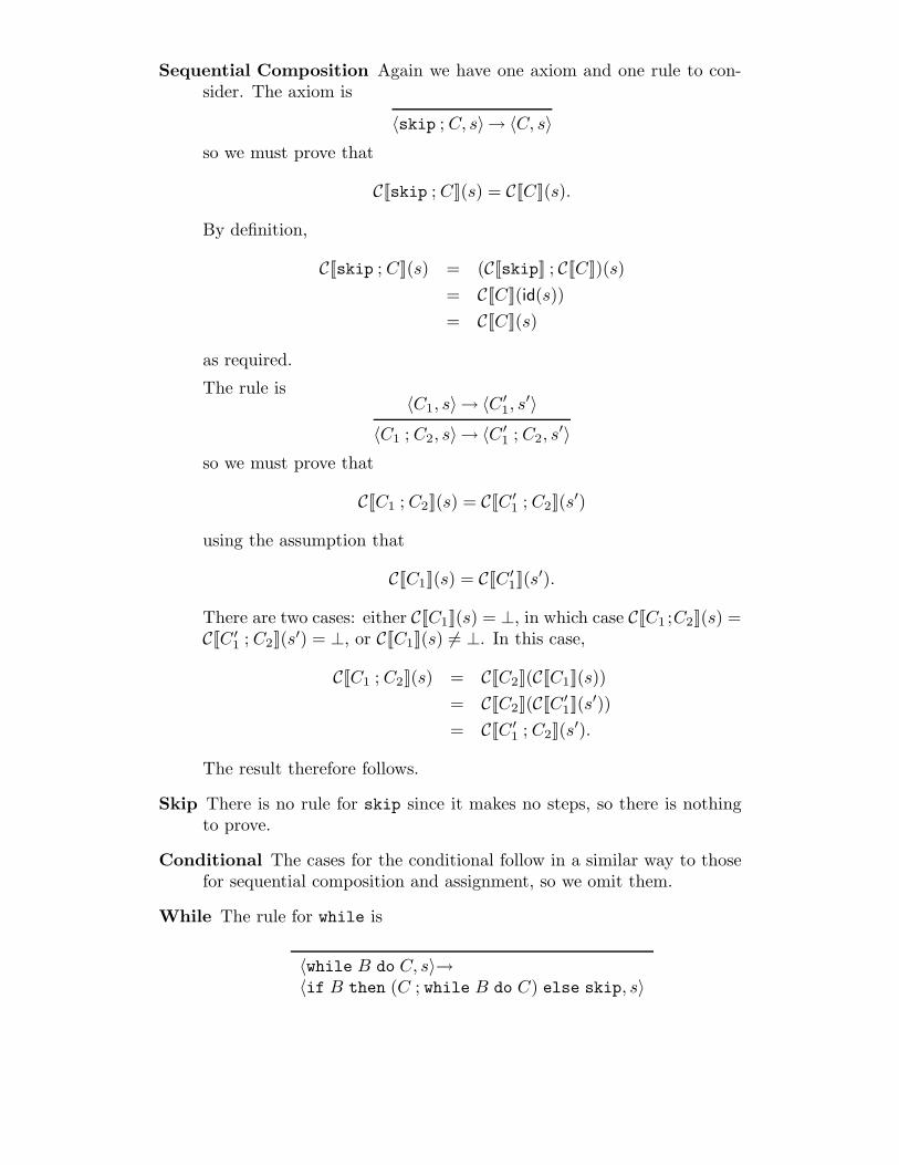
Sequential Composition Again we have one axiom and one rule to con-sider. The axiom is

〈skip ; C, s〉→ 〈C, s〉

so we must prove that

C[[skip ; C]](s) = C[[C]](s).

By definition,

C[[skip ; C]](s) = (C[[skip]] ; C[[C]])(s)

= C[[C]](id(s))

= C[[C]](s)

as required.

The rule is〈C1, s〉 → 〈C′

1, s′〉

〈C1 ; C2, s〉 → 〈C′

1 ; C2, s′〉

so we must prove that

C[[C1 ; C2]](s) = C[[C′

1 ; C2]](s′)

using the assumption that

C[[C1]](s) = C[[C′

1]](s′).

There are two cases: either C[[C1]](s) = ⊥, in which case C[[C1 ;C2]](s) =C[[C′

1 ; C2]](s′) = ⊥, or C[[C1]](s) 1= ⊥. In this case,

C[[C1 ; C2]](s) = C[[C2]](C[[C1]](s))

= C[[C2]](C[[C′

1]](s′))

= C[[C′

1 ; C2]](s′).

The result therefore follows.

Skip There is no rule for skip since it makes no steps, so there is nothingto prove.

Conditional The cases for the conditional follow in a similar way to thosefor sequential composition and assignment, so we omit them.

While The rule for while is

〈while B do C, s〉→〈if B then (C ; while B do C) else skip, s〉

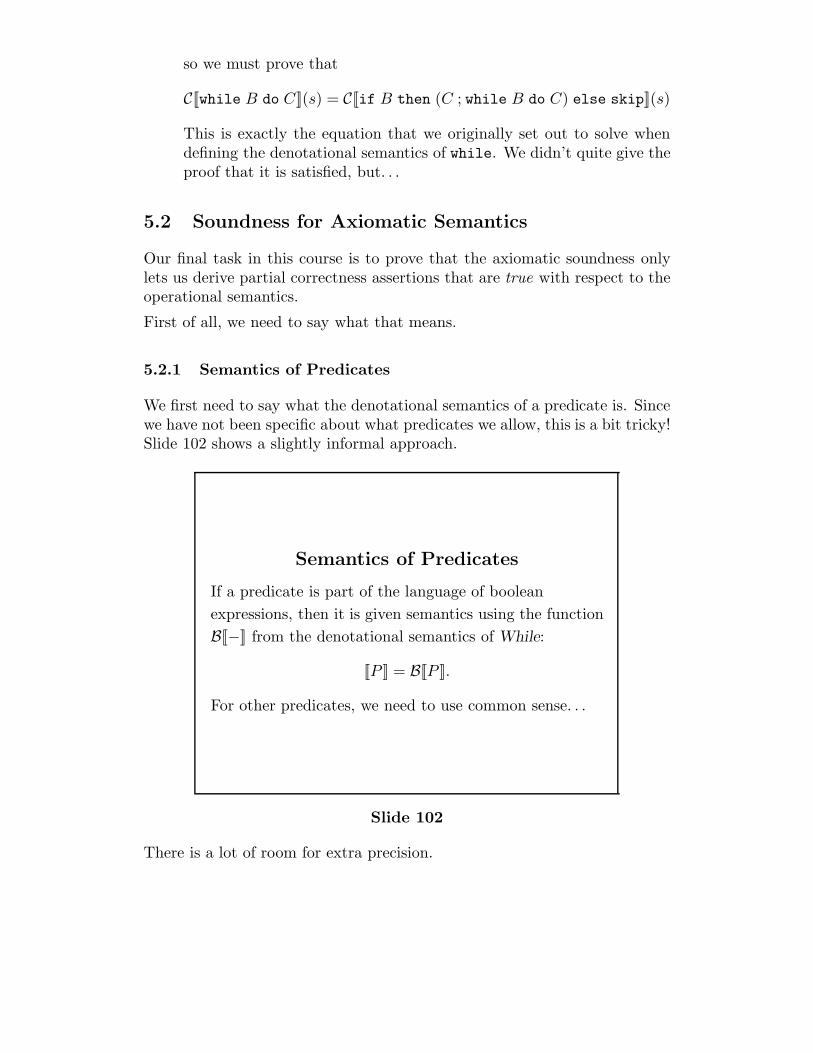
so we must prove that

C[[while B do C]](s) = C[[if B then (C ; while B do C) else skip]](s)

This is exactly the equation that we originally set out to solve whendefining the denotational semantics of while. We didn’t quite give theproof that it is satisfied, but. . .

5.2 Soundness for Axiomatic Semantics

Our final task in this course is to prove that the axiomatic soundness onlylets us derive partial correctness assertions that are true with respect to theoperational semantics.

First of all, we need to say what that means.

5.2.1 Semantics of Predicates

We first need to say what the denotational semantics of a predicate is. Sincewe have not been specific about what predicates we allow, this is a bit tricky!Slide 102 shows a slightly informal approach.

Semantics of Predicates

If a predicate is part of the language of boolean

expressions, then it is given semantics using the function

B[[−]] from the denotational semantics of While:

[[P ]] = B[[P ]].

For other predicates, we need to use common sense. . .

Slide 102

There is a lot of room for extra precision.

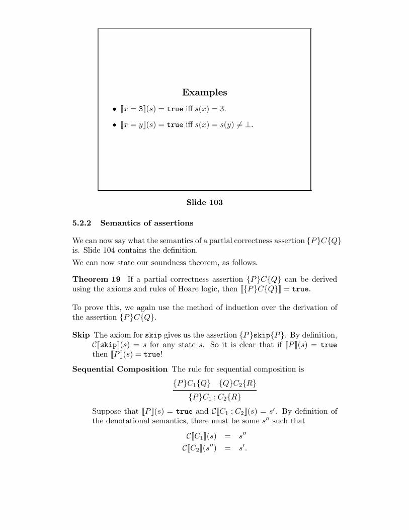
Examples

• [[x = 3]](s) = true iff s(x) = 3.

• [[x = y]](s) = true iff s(x) = s(y) 1= ⊥.

Slide 103

5.2.2 Semantics of assertions

We can now say what the semantics of a partial correctness assertion {P}C{Q}is. Slide 104 contains the definition.

We can now state our soundness theorem, as follows.

Theorem 19 If a partial correctness assertion {P}C{Q} can be derivedusing the axioms and rules of Hoare logic, then [[{P}C{Q}]] = true.

To prove this, we again use the method of induction over the derivation ofthe assertion {P}C{Q}.

Skip The axiom for skip gives us the assertion {P}skip{P}. By definition,C[[skip]](s) = s for any state s. So it is clear that if [[P ]](s) = truethen [[P ]](s) = true!

Sequential Composition The rule for sequential composition is

{P}C1{Q} {Q}C2{R}

{P}C1 ; C2{R}

Suppose that [[P ]](s) = true and C[[C1 ; C2]](s) = s′. By definition ofthe denotational semantics, there must be some s′′ such that

C[[C1]](s) = s′′

C[[C2]](s′′) = s′.

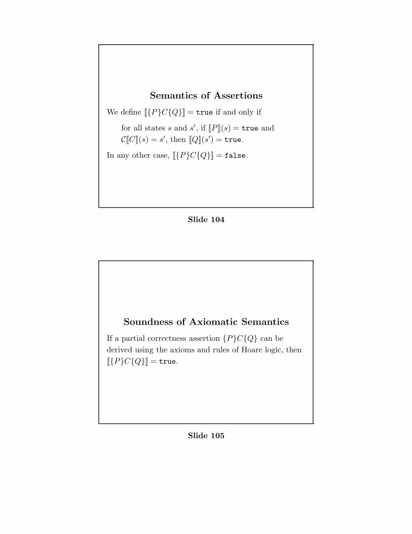
Semantics of Assertions

We define [[{P}C{Q}]] = true if and only if

for all states s and s′, if [[P ]](s) = true and

C[[C]](s) = s′, then [[Q]](s′) = true.

In any other case, [[{P}C{Q}]] = false.

Slide 104

Soundness of Axiomatic Semantics

If a partial correctness assertion {P}C{Q} can be

derived using the axioms and rules of Hoare logic, then

[[{P}C{Q}]] = true.

Slide 105

Using the inductive hypothesis, we know that [[{P}C1{Q}]] = true and[[{Q}C2{R}]] = true. This means that [[Q]](s′′) = true, and thereforethat [[R]](s′) = true as required.

Conditional The rule for the conditional is

{P ∧ B}C1{Q} {P ∧ ¬B}C2{Q}

{P}if B then C1 else C2{Q}.

Suppose that [[P ]](s) = true and C[[if B then C1 else C2]](s) = s′

for some states s and s′. There are two cases: either B[[B]](s) = trueor B[[B]](s) = false. (The only other possibility is that B[[B]](s) = ⊥,but then C[[if B then C1 else C2]](s) = ⊥ too, and we’ve assumedthat is not the case.)

• If B[[B]](s) = true then we know that [[P ∧ B]](s) = true, soapplying the inductive hypothesis to the first assertion above theline tells us that if C[[C1]](s) = s′′ then [[Q]](s′′) = true. Butin this case, we also know that C[[if B then C1 else C2]](s) =C[[C1]](s) = s′, so it follows that [[Q]](s′) = true as required.

• The case of B[[B]](s) = false is similar.

Assignment The axiom for assignment is

{Q[E/x]}x := E{Q}.

To prove that this is sound, we must prove that if [[Q[E/x]]](s) = truethen

[[Q]](s[x ,→ E [[E]](s)]) = true,

for every predicate Q, variable x, expression E and state s. To do thisproperly we would use induction on the structure of the predicate. Wehave not made the syntax of predicates precise, so we can’t do thatformally. We therefore omit a proof of this case, leaving it to yourintuition.

While The rule for while is

{P ∧ B}C{P}

{P}while B do C{P ∧ ¬B}

Let us suppose that [[P ]](s) = true and that C[[while B do C]](s) = s′.We must show that [[P ∧ ¬B]](s) = true, using the assumption that[[{P ∧ B}C{P}]] = true.

By definition of the semantics of while, s′ = C[[Ci]](s) for one of theapproximants Cn. It is therefore enough for us to show that the asser-tion

{P}Cn{P ∧ ¬B}

is semantically valid for each n. This we do by induction on n.

For the base case, since C[[C0]](s) = ⊥ always, there is nothing to prove.

For the inductive step, suppose that {P}Ck{P ∧ ¬B} is valid. Bydefinition, Ck+1 is the command

if B then C ; Ck else skip

and we need to show that {P}Ck+1{P ∧ ¬B} is semantically valid.Since we have already argued that the rules for skip, sequential com-position and conditional preserve semantic validity, we can use theserules to help us. The rule for conditional tells us that it will be enoughto show that both

{P ∧ B}C ; Ck{P ∧ ¬B}

and{P ∧ ¬B}skip{P ∧ ¬B}

are valid. The second of these obviously holds: it is an instance of therule for skip. For the first, the rule for sequential composition tells usthat it will be enough to find some predicate Q such that both

{P ∧ B}C{Q}

and{Q}Ck{P ∧ ¬B}

are valid.

But by the inductive hypothesis for this inner induction,

{P}Ck{P ∧ ¬B}

is valid, and by the inductive hypothesis for the outer induction, so is

{P ∧ B}C{P}.

So letting Q be P completes the inner induction, and hence the prooffor this case.

Logical rules The purely logical rules are very straightforward to verify, sowe omit their proofs.

So, both the operational and axiomatic semantics are correct with respectto the denotational semantics. We have therefore given an account of themeaning of simple programs in terms of state transformers which can beused to show that a simple kind of interpreter (the small-step semantics)works properly, and that certain reasoning principles (Hoare logic) are valid.Thus we have a reasonably complete semantic theory for these very simpleprograms.

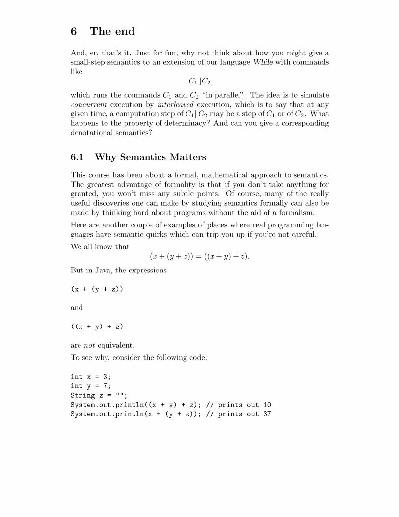
6 The end

And, er, that’s it. Just for fun, why not think about how you might give asmall-step semantics to an extension of our language While with commandslike

C1‖C2

which runs the commands C1 and C2 “in parallel”. The idea is to simulateconcurrent execution by interleaved execution, which is to say that at anygiven time, a computation step of C1‖C2 may be a step of C1 or of C2. Whathappens to the property of determinacy? And can you give a correspondingdenotational semantics?

6.1 Why Semantics Matters

This course has been about a formal, mathematical approach to semantics.The greatest advantage of formality is that if you don’t take anything forgranted, you won’t miss any subtle points. Of course, many of the reallyuseful discoveries one can make by studying semantics formally can also bemade by thinking hard about programs without the aid of a formalism.

Here are another couple of examples of places where real programming lan-guages have semantic quirks which can trip you up if you’re not careful.

We all know that(x + (y + z)) = ((x + y) + z).

But in Java, the expressions

(x + (y + z))

and

((x + y) + z)

are not equivalent.

To see why, consider the following code:

int x = 3;int y = 7;String z = "";System.out.println((x + y) + z); // prints out 10System.out.println(x + (y + z)); // prints out 37

Is this cheating? Not really: the semantics of + in Java is complicatedbecause it is an overloaded operator. As a programmer, you probably knewthis already. But if we gave a formal semantics to Java, we would have tomake the distinction between the numeric + and the string + explicit, sothat there was no confusion.

The second example illustrates the need to understand evaluation order,strictness and so on when programming.

Java’s && operator, for logical “and”, is a left-to-right, short-circuit operator.That is, in an expression

x && y

if x evaluates to false, Java does not evaluate y. However, method parame-ters are passed by value, which means they are always evaluated. Therefore,a method like

boolean logicalAnd(boolean x, boolean y) {return (x && y);

}

is not equivalent to &&. Can you come up with an example context to dis-tinguish them?

References

[NBB+63] Peter Naur, J. W. Backus, F. L. Bauer, J. Green, C. Katz, J. Mc-Carthy, A. J. Perlis, H. Rutishauer, K. Samelson, B. Vauquois,J. H. Wegstein, A. van Wijngaarden, and M. Woodger. Revisedreport on the algorithmic language ALGOL 60. Communicationsof the ACM, 6(1):1–17, January 1963.