Embed Size (px)
Citation preview
Semantic Similarity of Node Profiles in
Social Networks
A Dissertation Submitted to the
Graduate School
of the University of Cincinnati
in Partial Fulfillment of the
Requirements for the Degree of
Doctor of Philosophy
In the Department of
Electrical Engineering and Computing Systems
of College of Engineering and Applied Sciences
July 2015
By
Ahmad Y. Rawashdeh
M.S. Computer Science, Jordan University of Science and Technology, Jordan, January
2009
B.S. Computer Science, Jordan University of Science and Technology, Jordan, June 2006
Abstract
It can be said, without exaggeration, that social networks have taken a large segment of popu-
lation by a storm. Regardless of the actual geographical location, of socio-economic status, as long
as access to an internet connected computer is available, a person has access to the whole world,
and to a multitude of social networks. By being able to share, comment, and post on various social
networks sites, a user of social networks becomes a “citizen of the world”, ensuring presence across
boundaries (be they geographic, or socio-economic boundaries).
At the same time social networks have brought forward many issues interesting from computing
point of view. One of these issue is that of evaluating similarity between nodes/profiles in a social
network. Such evaluation is not only interesting, but important, as the similarity underlies the
formation of communities (in real life or on the web), of acquisition of friends (in real life and on
the web).
In this thesis, several methods for finding similarity, including semantic similarity, are investi-
gated, and a new approach, Wordnet-Cosine similarity is proposed. The Wordnet-Cosine similarity
(and associated distance measure) combines both a lexical database, Wordnet, with Cosine simi-
larity (from information retrieval) to find possible similar profiles in a network.
In order to assess the performance of Wordnet-Cosine similarity measure, two experiments
have been conducted. The first experiment illustrates the use for Wordnet-Cosine similarity in
community formation. Communities are considered to be clusters of profiles. The results of using
Wordnet-Cosine are compared with those using four other similarity measures (also described in
this thesis). In the second set of experiments, Wordnet-Cosine was applied to the problem of link
prediction. Its performance of predicting links in a random social graph was compared with a
random link predictor and was found to achieve better accuracy.
i

ii
Acknowledgements
This thesis marks the closing chapter of my study at the University of Cincinnati, where I spent
a wonderful time during which I learned a lot about research and teaching.
First, I would like to thank very much my adviser, Prof. Anca Ralescu, for her continuous
effort in advising me and guiding me through my Ph.D journey. She has taught me and helped me
understand difficult issues through numerous individual and group meetings. She never ceases to
surprise me with her gentle soul and her kind words. Her dedication to her students is something
that I can’t forget. I strongly recommend her to any student who is eager to learn and be inspired
to pursue her/his path through the field of Computer Science.
Thanks are due to the members of the PhD committee professors Ken Berman, Irene Diaz
Rodriguez, Rehab Duwairi, Chia Han, and Dan Ralescu for their agreement to be in my Ph.D
thesis committee, and valuable comments they made on the occasion of my proposal defense.
These comments guided my research at subsequent stages.
I gained valuable teaching experience as a Teaching Assistant for various Computer Science
courses. I was fortunate to work with the amazing professor Berman, professor Cheng, and again,
with my adviser, professor Ralescu.
Mrs. Julie Muenchen of Graduate Studies Office helped me with the procedures and regulations
toward completing all the requirements and for this I thank her too. I would like to thank my host
family Mrs. and Mr. Mary and Larry Collins. They welcomed me in their home and introduced
us to the wonderful American traditions. I made many friends among my group mates and other
students at the University of Cincinnati. I’m grateful to all for their friendship.
There is no better place and time to thank again my family. I’m grateful to my parents, my
mother Jamelah and my father Yousef, for their love and unconditional support. My dream of
achieving this moment in my studies became their dream.
iii

My heartfelt thanks and love go to my siblings, my elder brother, Mohammad the philosopher,
who preceded me in earning his PhD in Computer Science at University of Cincinnati, my lovely
and intelligent sister, Rabeah, PhD in nanotechnology, who has supported me for as long as I can
remember, and my younger brothers, Omar and Amer, biologist and mathematician respectively,
who bring joy and cheer us all.
iv
Contents
1 Introduction 1
1.1 The Similarity Problem in Social Network . . . . . . . . . . . . . . . . . . . . . . . . 1
1.1.1 Social Network and background . . . . . . . . . . . . . . . . . . . . . . . . . 1
Account . . . . . . . . . . . . . . . . . . . . . . . . . . . . . . . . . . . . . . . 2
Profile . . . . . . . . . . . . . . . . . . . . . . . . . . . . . . . . . . . . . . . . 2
Friends . . . . . . . . . . . . . . . . . . . . . . . . . . . . . . . . . . . . . . . 2
Search . . . . . . . . . . . . . . . . . . . . . . . . . . . . . . . . . . . . . . . . 3
Messages, Notifications, and Special Features . . . . . . . . . . . . . . . . . . 3
Limitations and Fellowship vs Friendship . . . . . . . . . . . . . . . . . . . . 4
1.1.2 Similarity . . . . . . . . . . . . . . . . . . . . . . . . . . . . . . . . . . . . . . 4
1.2 Organization of the Thesis . . . . . . . . . . . . . . . . . . . . . . . . . . . . . . . . . 5
2 Initial Experiment 6
2.1 Initial Experiment . . . . . . . . . . . . . . . . . . . . . . . . . . . . . . . . . . . . . 6
2.1.1 Related Work on Similarity . . . . . . . . . . . . . . . . . . . . . . . . . . . . 6
2.1.2 Datasets . . . . . . . . . . . . . . . . . . . . . . . . . . . . . . . . . . . . . . . 10
Facebook Dataset . . . . . . . . . . . . . . . . . . . . . . . . . . . . . . . . . 10
The authorship dataset (DBLP) . . . . . . . . . . . . . . . . . . . . . . . . . 11
2.1.3 Initial System Architecture . . . . . . . . . . . . . . . . . . . . . . . . . . . . 11
2.1.4 Results of Initial Experiments . . . . . . . . . . . . . . . . . . . . . . . . . . . 12
2.1.5 Conclusion for Chapter 2 . . . . . . . . . . . . . . . . . . . . . . . . . . . . . 12
v
3 Similarity Between Nodes in a Social Network 14
3.1 Similarity in Social Networks . . . . . . . . . . . . . . . . . . . . . . . . . . . . . . . 15
3.2 Semantic Similarity . . . . . . . . . . . . . . . . . . . . . . . . . . . . . . . . . . . . . 16
3.3 Problem description and evaluation metrics . . . . . . . . . . . . . . . . . . . . . . . 18
3.4 Motivation for finding similarity . . . . . . . . . . . . . . . . . . . . . . . . . . . . . 18
3.5 Node and other similarity measurements . . . . . . . . . . . . . . . . . . . . . . . . . 19
3.5.1 Node Similarity . . . . . . . . . . . . . . . . . . . . . . . . . . . . . . . . . . . 20
3.5.2 Edge similarity . . . . . . . . . . . . . . . . . . . . . . . . . . . . . . . . . . . 21
3.5.3 Global Structural Similarities . . . . . . . . . . . . . . . . . . . . . . . . . . . 22
3.5.4 Conclusion for Chapter 3 . . . . . . . . . . . . . . . . . . . . . . . . . . . . . 23
4 Semantic Similiarity Measures 26
4.1 Similarity measures and Semantic . . . . . . . . . . . . . . . . . . . . . . . . . . . . . 27
4.2 Finding Similar Profiles . . . . . . . . . . . . . . . . . . . . . . . . . . . . . . . . . . 27
4.2.1 Wordnet . . . . . . . . . . . . . . . . . . . . . . . . . . . . . . . . . . . . . . . 27
Hypernym of a word . . . . . . . . . . . . . . . . . . . . . . . . . . . . . . . . 27
Wordnet Java API . . . . . . . . . . . . . . . . . . . . . . . . . . . . . . . . . 28
4.2.2 Semantic Tagger . . . . . . . . . . . . . . . . . . . . . . . . . . . . . . . . . . 28
4.2.3 The occurrence frequency similarity(OF) . . . . . . . . . . . . . . . . . . . . 29
4.3 A unified Similarity Measure: Wordnet-cosine similarity . . . . . . . . . . . . . . . . 29
4.4 Experimental Results . . . . . . . . . . . . . . . . . . . . . . . . . . . . . . . . . . . . 30
4.4.1 Facebook profiles data-set . . . . . . . . . . . . . . . . . . . . . . . . . . . . . 31
4.4.2 Results . . . . . . . . . . . . . . . . . . . . . . . . . . . . . . . . . . . . . . . 31
4.5 Conclusion for Chapter 4 . . . . . . . . . . . . . . . . . . . . . . . . . . . . . . . . . 35
5 Algorithms and Implementations for Finding Similarity 36
5.1 Java algorithms for finding similarities . . . . . . . . . . . . . . . . . . . . . . . . . . 36
5.1.1 Time Complexity Analysis of the Similarity Algorithms . . . . . . . . . . . . 47
5.1.2 Space complexity of the similarity algorithms . . . . . . . . . . . . . . . . . . 48
vi
6 Experiments and Results 49
6.1 Experiments . . . . . . . . . . . . . . . . . . . . . . . . . . . . . . . . . . . . . . . . . 49
6.2 Creating the similarity and Distance Matrices . . . . . . . . . . . . . . . . . . . . . . 54
6.3 Clustering using Similarity and the Silhouette Index for Clustering Validation . . . . 57
6.3.1 Kmeans Clustering . . . . . . . . . . . . . . . . . . . . . . . . . . . . . . . . . 57
6.3.2 Silhouette . . . . . . . . . . . . . . . . . . . . . . . . . . . . . . . . . . . . . . 57
6.3.3 Facebook . . . . . . . . . . . . . . . . . . . . . . . . . . . . . . . . . . . . . . 58
Set Distance . . . . . . . . . . . . . . . . . . . . . . . . . . . . . . . . . . . . 58
Wordnet-Cosine Distance . . . . . . . . . . . . . . . . . . . . . . . . . . . . . 58
Semantic Categories Distance . . . . . . . . . . . . . . . . . . . . . . . . . . . 58
Word Frequency Vector Distance . . . . . . . . . . . . . . . . . . . . . . . . . 58
Average Silhouette . . . . . . . . . . . . . . . . . . . . . . . . . . . . . . . . . 59
6.3.4 DBLP . . . . . . . . . . . . . . . . . . . . . . . . . . . . . . . . . . . . . . . . 59
Set Distance . . . . . . . . . . . . . . . . . . . . . . . . . . . . . . . . . . . . 60
Wordnet-Cosine Distance . . . . . . . . . . . . . . . . . . . . . . . . . . . . . 60
Semantic Categories Distance . . . . . . . . . . . . . . . . . . . . . . . . . . . 60
Word Frequency Vector Distance . . . . . . . . . . . . . . . . . . . . . . . . . 61
Average Silhouette . . . . . . . . . . . . . . . . . . . . . . . . . . . . . . . . . 61
6.3.5 Movielens . . . . . . . . . . . . . . . . . . . . . . . . . . . . . . . . . . . . . . 62
Set Distance . . . . . . . . . . . . . . . . . . . . . . . . . . . . . . . . . . . . 62
Wordnet-Cosine Distance . . . . . . . . . . . . . . . . . . . . . . . . . . . . . 62
Semantic Categories Distance . . . . . . . . . . . . . . . . . . . . . . . . . . . 62
Word Frequency Vector Distance . . . . . . . . . . . . . . . . . . . . . . . . . 63
Average Silhouette . . . . . . . . . . . . . . . . . . . . . . . . . . . . . . . . . 63
6.4 Comparison between Different Measures . . . . . . . . . . . . . . . . . . . . . . . . . 64
6.5 Correlation between the Similarity Measures . . . . . . . . . . . . . . . . . . . . . . . 66
6.6 Link Prediction using the Wordnet-Cosine similarity/distance measure . . . . . . . . 66
6.6.1 Wordnet-Cosine and Random Graph Adjacency . . . . . . . . . . . . . . . . . 76
6.7 Conclusion to Chapter 6 . . . . . . . . . . . . . . . . . . . . . . . . . . . . . . . . . . 77
vii
7 Conclusion 85
8 Appendix 87
8.1 Code . . . . . . . . . . . . . . . . . . . . . . . . . . . . . . . . . . . . . . . . . . . . . 87
8.1.1 Clustering Code . . . . . . . . . . . . . . . . . . . . . . . . . . . . . . . . . . 87
8.1.2 Avg Silhouette Code . . . . . . . . . . . . . . . . . . . . . . . . . . . . . . . . 87
8.1.3 Modified Kmeans (KernelKmean) Code . . . . . . . . . . . . . . . . . . . . . 88
8.1.4 Link Prediction Experiment . . . . . . . . . . . . . . . . . . . . . . . . . . . . 88
8.2 System specification . . . . . . . . . . . . . . . . . . . . . . . . . . . . . . . . . . . . 88
viii
List of Figures
2.1 Small network with node profiles expressed as strings of characters. . . . . . . . . . . 10
2.2 Usage - Link prediction on the network illustrated in Figure 2.1when node profile
similarities are computed with the Jaccard index. . . . . . . . . . . . . . . . . . . . . 10
2.3 Frequencies of the top 20 Movies interest in the Facebook dataset . . . . . . . . . . . 11
2.4 Architecture . . . . . . . . . . . . . . . . . . . . . . . . . . . . . . . . . . . . . . . . . 12
2.5 Results (Similarity Histograms)- Facebook dataset . . . . . . . . . . . . . . . . . . . 13
2.6 Results (Similarity Histogram) - DBLP dataset . . . . . . . . . . . . . . . . . . . . . 13
4.1 Histogram of OF and Wordnet similarity using the Facebook dataset. . . . . . . . . 34
4.2 Histogram of the four similarity measures using the Facebook dataset. . . . . . . . . 34
5.1 Dependency between the procedures used to find the similarity measure . . . . . . . 38
5.2 Dependency between the procedures used to find the Word Frequency Vector measure 38
6.1 Histogram of distances of Facebook data for the four similarity measures . . . . . . . 51
6.2 Histogram of Distances of MovieLens data for the four Similarity Measures . . . . . 52
6.3 Histogram of Distances of DBLP data for the four Similarity Measures . . . . . . . . 53
6.4 The Image Plots of Facebook Distance Matrices . . . . . . . . . . . . . . . . . . . . . 54
6.5 Clustering using Set Distance applied on Facebook Dataset . . . . . . . . . . . . . . 59
6.6 Clustering using Wordnet-Cosine Distance applied on Facebook Dataset . . . . . . . 59
6.7 Clustering using Semantic Categories Distance applied on Facebook Dataset . . . . 59
6.8 Clustering using Word Frequency Vector Distance applied on Facebook Dataset . . 60
6.9 Average Silhouette for clustering the Facebook Dataset into 1-6 Clusters using dif-
ferent Distance Measures . . . . . . . . . . . . . . . . . . . . . . . . . . . . . . . . . 60
ix
6.10 Clustering using Set distance applied on DBLP Dataset . . . . . . . . . . . . . . . . 61
6.11 Clustering using Wordnet-Cosine Distance applied on DBLP Dataset . . . . . . . . 61
6.12 Clustering using Semantic Categories Distance applied on DBLP Dataset . . . . . . 61
6.13 Clustering using Word Frequency Vector Distance applied on DBLP Dataset . . . . 62
6.14 Average Silhouette for clustering the DBLP dataset into 1-6 clusters using Different
Distance Measures . . . . . . . . . . . . . . . . . . . . . . . . . . . . . . . . . . . . . 62
6.15 Clustering using Set distance applied on Movielen Dataset . . . . . . . . . . . . . . 63
6.16 Clustering using Wordnet-Cosine distance applied on Movielen Dataset . . . . . . . 63
6.17 Clustering using Semantic Categories Distance applied on Movielen Dataset . . . . 63
6.18 Clustering using Word Frequency Vector Distance applied on Movielen Dataset . . 64
6.19 Average Silhouette for clustering the Movielen dataset into 1-6 Clusters using Dif-
ferent Distance Measures . . . . . . . . . . . . . . . . . . . . . . . . . . . . . . . . . 64
6.20 Correlation between the Number of Common Friends’ Interests and Jaccard . . . . . 67
6.21 Random Graph . . . . . . . . . . . . . . . . . . . . . . . . . . . . . . . . . . . . . . . 68
6.22 Histogram of accuracies for the Random and Wordnet-Cosine distance predictors. . . 75
6.23 Accuracy of Wordnet-Cosine Distance Predictor. . . . . . . . . . . . . . . . . . . . . 75
6.24 Accuracy of Random Predictor. . . . . . . . . . . . . . . . . . . . . . . . . . . . . . . 76
6.25 Difference between the accuracy of Wordnet-Cosine Distance and Random Predictor 77
6.26 Number of Different Elements between the modified Wordnet-Cosine distance matrix
and Random Graph Adjacency matrix . . . . . . . . . . . . . . . . . . . . . . . . . . 77
6.27 Percentage of difference between the modified Wordnet-Cosine distance matrix and
Random Graph adjacency . . . . . . . . . . . . . . . . . . . . . . . . . . . . . . . . . 78
8.1 Clustering the D Cat FD N F matrix (the Semantic Categoriy distance matrix) . . . 87
8.2 Code for finding the Average Silhouette using the modified kmeans, KernelKmean . 88
8.3 KernelKmean: the modified Kmeans which takes a distance matrix as an input . . . 90
8.4 Link Prediction Experiment - part 1 . . . . . . . . . . . . . . . . . . . . . . . . . . . 91
8.5 Link Prediction Experiment - part 2 . . . . . . . . . . . . . . . . . . . . . . . . . . . 92
8.6 Link Prediction Experiment - part 3 . . . . . . . . . . . . . . . . . . . . . . . . . . . 93
8.7 Link Prediction Experiment - part 4 (a) . . . . . . . . . . . . . . . . . . . . . . . . . 94
x
8.8 Link Prediction Experiment - part 4 (b) . . . . . . . . . . . . . . . . . . . . . . . . . 95
8.9 Link Prediction Experiment - part 4 (c) . . . . . . . . . . . . . . . . . . . . . . . . . 96
8.10 Link Prediction Experiment - part 4 (d) . . . . . . . . . . . . . . . . . . . . . . . . . 96
8.11 Link Prediction Experiment - part 4 (e) . . . . . . . . . . . . . . . . . . . . . . . . . 97
8.12 System Specifications . . . . . . . . . . . . . . . . . . . . . . . . . . . . . . . . . . . . 98
xi
List of Tables
1.1 Comparison between different social networks . . . . . . . . . . . . . . . . . . . . . . 4
2.1 Pairwise similarity values for the network in Figure 2.1. . . . . . . . . . . . . . . . . 9
2.2 Statistics of the Facebook Dataset . . . . . . . . . . . . . . . . . . . . . . . . . . . . 11
3.1 Two Facebook profiles . . . . . . . . . . . . . . . . . . . . . . . . . . . . . . . . . . . . 20
3.2 Node and Link similarities . . . . . . . . . . . . . . . . . . . . . . . . . . . . . . . . . 22
3.3 Comparison between similarity measures . . . . . . . . . . . . . . . . . . . . . . . . . 24
3.4 Comparison between similarity measures . . . . . . . . . . . . . . . . . . . . . . . . . . 25
4.1 Word tags and their descriptions [6]. . . . . . . . . . . . . . . . . . . . . . . . . . . . 28
4.2 The cosine similarity of vectors v . . . . . . . . . . . . . . . . . . . . . . . . . . . . . 31
4.3 Illustration of Movie Attribute of Facebook profiles: their tags and Hypernyms. . . . 32
4.4 OF and Wordnet-Cosine similarity of two Facebook profiles along their Movie At-
tribute. Profile IDs are partially masked for privacy. . . . . . . . . . . . . . . . . . . 32
4.5 User rating of the similarity between profile 1 and profile 2 using Facebook dataset
in table 4.4 . . . . . . . . . . . . . . . . . . . . . . . . . . . . . . . . . . . . . . . . . 33
4.6 Genres for movies listed in Table 4.4 . . . . . . . . . . . . . . . . . . . . . . . . . . . 33
5.1 Running time complexity of the similarity algorithms . . . . . . . . . . . . . . . . . . 48
6.1 The Format for the Movielens Dataset . . . . . . . . . . . . . . . . . . . . . . . . . . 50
6.2 Facebook Dataset: the First 10 Records . . . . . . . . . . . . . . . . . . . . . . . . . 50
6.13 Accuracy of Wordnet-Cosine and Random Predictors . . . . . . . . . . . . . . . . . . 70
6.3 MovieLens Dataset: the First 10 Records . . . . . . . . . . . . . . . . . . . . . . . . 79
xii
6.4 DBLP Dataset: the First 10 Records . . . . . . . . . . . . . . . . . . . . . . . . . . . 79
6.5 Characteristic of Distance Matrices used for Clustering . . . . . . . . . . . . . . . . 80
6.6 Distance Data Matrices from the Facebok Dataset ( FD) . . . . . . . . . . . . . . . 80
6.7 Extended Facebook dataset for User whose id is 1 . . . . . . . . . . . . . . . . . . . 81
6.8 Extended Facebook Dataset Statistics . . . . . . . . . . . . . . . . . . . . . . . . . . 82
6.9 Sample results - Common Movies Interest between the Friends of two Facebook Users
identified by ids 305 and 389 . . . . . . . . . . . . . . . . . . . . . . . . . . . . . . . 82
6.10 More Comparison between the Similarity Measures for two Facebook Profiles iden-
tified by ids 441 and 134 . . . . . . . . . . . . . . . . . . . . . . . . . . . . . . . . . 83
6.11 Correlation between Different Measures . . . . . . . . . . . . . . . . . . . . . . . . . 83
6.12 Comparison between Wordnet-Cosine and Random Predictors for DistT = 10 . . . . 84
6.14 Comparison between Random Accuracy and Wordnet-Cosine distance Accuracy when
Distance Threshold = 60 and for different values of % edges deleted . . . . . . . . . 84
6.15 Difference between the modified Wordnet-Cosine distance and the Random Grahp
adjacency matrix . . . . . . . . . . . . . . . . . . . . . . . . . . . . . . . . . . . . . . 84
8.1 System Specification . . . . . . . . . . . . . . . . . . . . . . . . . . . . . . . . . . . . 88
8.2 Used software . . . . . . . . . . . . . . . . . . . . . . . . . . . . . . . . . . . . . . . . 89
xiii
Chapter 1
Introduction
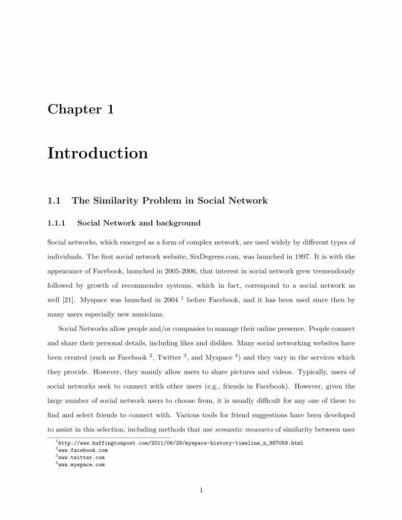
1.1 The Similarity Problem in Social Network
1.1.1 Social Network and background
Social networks, which emerged as a form of complex network, are used widely by different types of
individuals. The first social network website, SixDegrees.com, was launched in 1997. It is with the
appearance of Facebook, launched in 2005-2006, that interest in social network grew tremendously
followed by growth of recommender systems, which in fact, correspond to a social network as
well [21]. Myspace was launched in 2004 1 before Facebook, and it has been used since then by
many users especially new musicians.
Social Networks allow people and/or companies to manage their online presence. People connect
and share their personal details, including likes and dislikes. Many social networking websites have
been created (such as Facebook 2, Twitter 3, and Myspace 4) and they vary in the services which
they provide. However, they mainly allow users to share pictures and videos. Typically, users of
social networks seek to connect with other users (e.g., friends in Facebook). However, given the
large number of social network users to choose from, it is usually difficult for any one of these to
find and select friends to connect with. Various tools for friend suggestions have been developed
to assist in this selection, including methods that use semantic measures of similarity between user
1http://www.huffingtonpost.com/2011/06/29/myspace-history-timeline_n_887059.html2www.facebook.com3www.twitter.com4www.myspace.com
1
profiles in the network. In addition to suggesting friends or followers in social network, methods for
suggesting items to buy may be investigates in retail websites (such as Amazon 5). Such methods
are based on an implicit social network of users who buy similar items, as tracked by Amazon.
Facebook allows users to search for friends within a geographical area (e.g. Cincinnati), univer-
sity, work place, living place, as well as by using other attributes. Some social networks websites ask
for the login information of email services (Yahoo or GMail) in order to connect with the contacts
from the user email account, and build the friends list for the new users (newbie).
Account
A social network user must have an account which is created by choosing a username, password,
and providing the website with a valid email address. After that, the newly registered user fills
up the profile with personal information and connects with friends. The privacy setting can be
customized using various privacy options (e.g. in Facebook: Family, friends, close friends, etc).
Profile
The user profile page, lists, aside from his/her personal information, the connections (friends in
Facebook, followers in Twitter, etc) that the user has. In particular, in Facebook, the profile shows,
depending on the privacy setting chosen by the user, the personal information (birthday, name, and
possibly the phone number), likes, friends, interests (movies, TV shows, etc), and the wall posts.
Each user has a wall that shows friends’ posts, in which the user was tagged, and also the profile
owner’s posts. Twitter profile shows the tweets by the user, favorites, connections (followers and
followed), pictures and videos posted by the user. A twitter user can protect his/her tweets from
being visible to the public by adjusting the corresponding settings so that only confirmed followers
can see them.
Friends
Facebook limits the number of friends to 5000 6 while Twitter has an initial limit of people to follow
of 2000. If the user wants to follow more than this limit, (s)he can follow only 10% of his followers
5www.amazon.com6https://www.facebook.com/help/community/question/?id=10151800679568529
2
(for example a user with 15,000 followers is allowed to follow 3000). 7
Search
In order to search for friends in Facebook, the user can specify the value of different search criteria
such as: Name, Hometown, Current City, High School, Mutual Friend, College, Employer, and
Graduate School. A Facebook or Twitter user can also add a friend by providing his/her email
address, as mentioned previously. The objective of the work described here is to improve the ”People
you May Know” service in Facebook, ”Customers who bought this item also bought” service in
Amazon, and ”People who liked this also liked” service in IMDB 8, and any similar feature which
helps in avoiding searching a large amount of data and tackles the problem of finding the right
match between user profiles, by suggesting those who might be similar or items that might be of
interest.
Messages, Notifications, and Special Features
Most Social Networking websites support messaging between users which allows them to have a
private conversation in addition to the public communication they post on their profile pages. In
Facebook and Twitter more than one person can be selected to receive a message by simply typing
their usernames in the message-to field.
In Facebook, automatic notifications let users know about activities of their connections. These
notifications can be customized to meet the user needs. For instance, one can choose whether to
receive notification from a group (every time a user posts in that group) or an individual. Basically
”Following” a user leads to receiving notification of the user actions. Facebook allows users to view
the latest activities log: comments, friendship request and acceptance, likes, etc. Facebook provides
the users the option for creating special purpose groups which can be closed or open. Members of
the same group can share their post on the group and communicate with each other.
7http://blog.justunfollow.com/2014/03/13/10-twitter-limits-any-smart-user-should-know/8www.imdb.com
3
Limitations and Fellowship vs Friendship
Twitter users fall into two categories, content providers (also known as followees) and content
consumers (also known as followers). A Twitter user is usually both a follower and a followee.
Moroever, in contrast to Facebook, Twitter limits the number of characters that can be posted:
people post tweets limited to 140 characters, Facebook status messages have a much larger limit
(as of 2011 they were extended to approximately 60,000 characters 9). In Facebook a link/friend
connection between two users can be established only upon mutual agreement, while in Twitter,
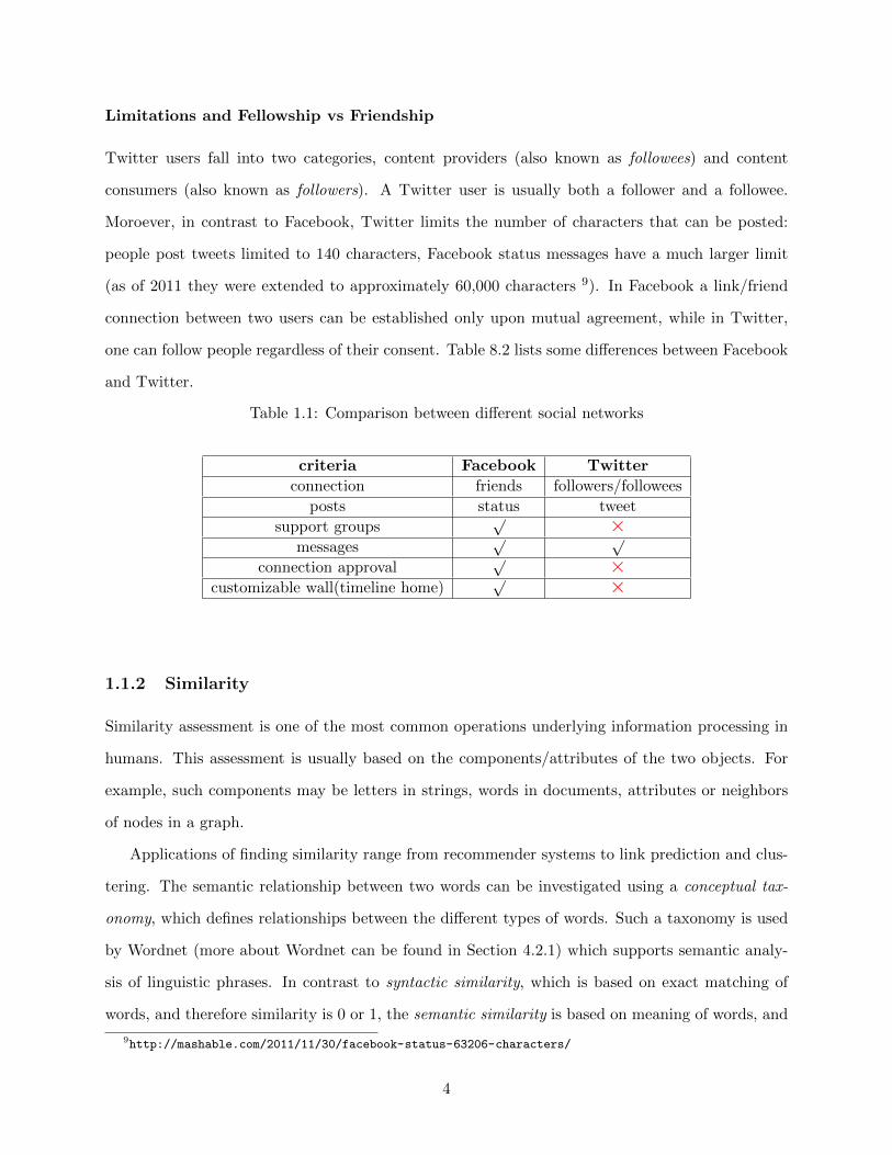
one can follow people regardless of their consent. Table 8.2 lists some differences between Facebook
and Twitter.
Table 1.1: Comparison between different social networks
criteria Facebook Twitter
connection friends followers/followees
posts status tweet
support groups√ ×
messages√ √
connection approval√ ×
customizable wall(timeline home)√ ×
1.1.2 Similarity
Similarity assessment is one of the most common operations underlying information processing in
humans. This assessment is usually based on the components/attributes of the two objects. For
example, such components may be letters in strings, words in documents, attributes or neighbors
of nodes in a graph.
Applications of finding similarity range from recommender systems to link prediction and clus-
tering. The semantic relationship between two words can be investigated using a conceptual tax-
onomy, which defines relationships between the different types of words. Such a taxonomy is used
by Wordnet (more about Wordnet can be found in Section 4.2.1) which supports semantic analy-
sis of linguistic phrases. In contrast to syntactic similarity, which is based on exact matching of
words, and therefore similarity is 0 or 1, the semantic similarity is based on meaning of words, and
9http://mashable.com/2011/11/30/facebook-status-63206-characters/
4
therefore results in similarity value in [0,1], which helps in enhancing information retrieval.
This work investigates a semantic similarity measure on the content of social network. It defines
a unified similarity measure where a node profile is represented as a semantic vector of semantic
entities extracted according to Wordnet. A new similarity measure is proposed by evaluating the
cosine similarity between these semantic vectors. Its performance is compared with other similarity
measure on several datasets.
1.2 Organization of the Thesis
This thesis is organized as follows: first, an introduction about Social network and similarity
was included in Chapter 1, which is followed by details about an initial experiment in Chapter
2. Chapter 3 surveys different types of similarities. Then a comparison between four selected
similarity measures is included in Chapter 4 as well as some results. Chapter 5 includes Algorithmic
description for each of the four similarity measures. After that, in depth overview of the two sets
of experiments conducted to evaluate the different similarity measures is included in Chapter 6.
Finally, the conclusion and future work.
5
Chapter 2
Initial Experiment
2.1 Initial Experiment
To begin with, an experiment was conducted to assess the proposed similarity measure, Wordnet-
Cosine, against the Occurrence Frequency (OF) similarity (more about the OF can be found in
Section 4.2.3). For this purpose, two data sets were used as follows: Facebook dataset, containing
the movies interest of users, found in a list known as SkullSecurity [5], and a dataset from the
DBLP site [2], which contains the publication titles for scientific/scholarly papers.
2.1.1 Related Work on Similarity
Analysis of similarity between Facebook profiles can be assessed from the study of keyword similarity
[12]. To find the relationship between the keywords,they were arranged in a hierarchical structure
to form trees of possibly different heights. In the forest model, more than one tree was generated
for each profile. A set of heuristics to retrieve the related words was used. The four heuristics are
• Base: The tree is composed only of the initial keyword.
• Holonyms/Meronyms (HM): The whole/part description
• Synonym/Similar (SS)
• ALL: using all of the previous descriptions
Wordnet was used to find the semantic relationship between the words. [12]
6
The semantic distance between profiles is very important to this process, as it has been shown
that the similarity between profiles deteriorates as the distance between them increases. Manhattan
and Euclidean distance are independent of the distribution underlying the data set. It was shown
that when similarity is dependent of this distribution, no single measure is superior [14].
The approach taken in this thesis does not depend on the distribution underlying the dataset.
Barbara, et al proposed a method of network similarity that only depends on the structure of the
dataset and profile similarity measures, and a method for inferring missing items. They used the oc-
currence frequency because it produces values in the interval [0, 1] according to how similar profiles
are, based on the frequency of the items in the dataset [8]. In contrast to the Inverse Occurrence
Frequency (IOF), less frequent mismatches are assigned lower similarity when using the Occurrence
Frequency (OF), while mismatches on high frequent values are assigned higher similarity. The simi-
larity measures are classified according to which part of the similarity matrix they fill with weighted
values (not equally assigning a single value of 0 or 1). The diagonal similarity measures assigns 0
as the similarity values for all mismatches and a weighted similarity for matches. The off diagonal
measures, assign 1 as the similarity values for all matches and a different weights to mismatches.
Both ways produce weighted values for matches (diagonal) and mismatches (offdiagonal). OF is
one of the measures that has best performance in detecting outliers. Outliers detection could be
used as a measure for evaluating the approach taken in this thesis, by adding the outliers, feature
values that are far away from the top concept in the semantic hierarchy, to the test set. Then the
k nearest neighbors are found using the Wordnet-Cosine (proposed in this thesis) algorithm and
the occurrence frequency method, in a way similar to [14]
Link prediction can be approached using three measures based on, respectively, (1) the topo-
logical structure of the data, (2) the profile information, and (3) combination of both [42]. It
has been found that algorithms based on topological structure of profiles and techniques based on
user-created similarity perform better at suggesting new links/friends.
The Inter-Profile Similarity (IPS) algorithm [53] utilizes Natural Language Processing (NLP)
to find similar social network profiles based on the approximate matching of phrases. It includes
ProfileSimilarity, a measure which takes two short snippets from two profiles (respectively, A and
B) and performs word sense disambiguation first. Then it finds the meaning of each snippet, which
will be used to find the similarity between them, a value in [0, 1]. A user study was conducted to
7
evaluate the algorithm. The authors report that the approach suffers from “few shortcomings that
need to be solved”. The IPS algorithm was also compared with the simple intersection approach
of finding similar profiles. The main concern was the change in the semantic similarity with the
distance between profiles. Enhancement of the profile semantic similarity was one of the motivations
for the approach presented in this thesis.
Similarity evaluation is an important aspect for recommending online communities to the users.
For example, in [54], six different measures of similarity (including L1- and L2- norms) for recom-
mending online communities were evaluated, based on using the information of visit and join to
communities. However, no semantic information or NLP tools were used.
An adaptation of the Occurrence Frequency is described in [9] which produces 1 for identical
values and a non-zero value for distinct item values (dissimilarity). In addition, the approach takes
into account the distribution of the values in the dataset.
Missing Values
The simple approach of giving high similarity value for profiles with similar feature values, and
low similarity for dissimilar values, results in low similarity values for profiles with missing values.
Using the network information to predict missing values is not accurate and it cannot distinguish
between cases of missing values, and the “doesn’t apply” situation for an attribute. To calculate
f(x), the frequency of feature value x, instead of the number of records in friends list that have
the value x (as done in [9]), in this thesis, the number of records in the dataset with the value x is
used, which leads to higher OF similarity values.
Clustering
Clustering techniques can be used for link suggestion/prediction. However, similarity/distance
evaluation underlies such techniques. In [16] graph clustering and relational clustering were used
for link suggestion. To take into account profile information, dummy vertices were added to the
original graph to represent attribute values, converting this way, profile information into graph
structure information. A unified neighborhood random walk was then performed on the resulting
graph. Node profile information was used in a syntactic manner (exact matching of words), and
no NLP tools (such as a tagger) were used. Semantic similarity could be added to this approach
8
resulting in a graph with a simpler structure (e.g., smaller number of nodes).
In another departure from previous work, this thesis investigates semantic relationship between
attribute entries in the social network, not only between keywords. Therefore the category of a
word must be found. This can be accomplished by using a tagger, a program which tags a word by
its part of speech category [3]. The categories used in this study are: NN (noun, proper, singular
or mass), NNP (noun, proper, singular), NNS (noun, common, plural), and NNPS (noun, proper,
plural) [6]. These part of speech tags are used to assess profile similarity. This research improves
on finding the similarity between profiles using the semantic distance between attribute entries
by using Wordnet as a lexical database. The approach taken here is illustrated on two datasets,
Facebook and DBLP. Before proceeding further, Example 2.1.1 illustrates similarity-based link
prediction in a network.
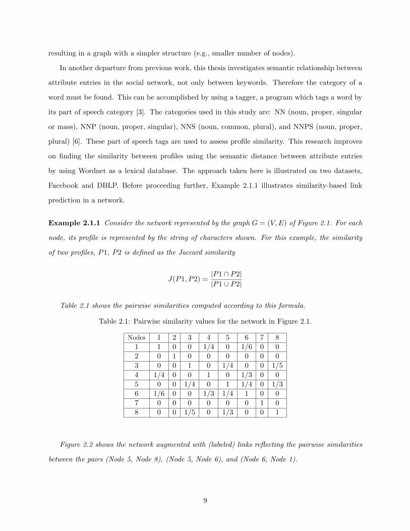
Example 2.1.1 Consider the network represented by the graph G = (V,E) of Figure 2.1. For each
node, its profile is represented by the string of characters shown. For this example, the similarity
of two profiles, P1, P2 is defined as the Jaccard similarity
J(P1, P2) =|P1 ∩ P2||P1 ∪ P2|
Table 2.1 shows the pairwise similarities computed according to this formula.
Table 2.1: Pairwise similarity values for the network in Figure 2.1.
Nodes 1 2 3 4 5 6 7 8
1 1 0 0 1/4 0 1/6 0 0
2 0 1 0 0 0 0 0 0
3 0 0 1 0 1/4 0 0 1/5
4 1/4 0 0 1 0 1/3 0 0
5 0 0 1/4 0 1 1/4 0 1/3
6 1/6 0 0 1/3 1/4 1 0 0
7 0 0 0 0 0 0 1 0
8 0 0 1/5 0 1/3 0 0 1
Figure 2.2 shows the network augmented with (labeled) links reflecting the pairwise similarities
between the pairs (Node 5, Node 8), (Node 5, Node 6), and (Node 6, Node 1).
9
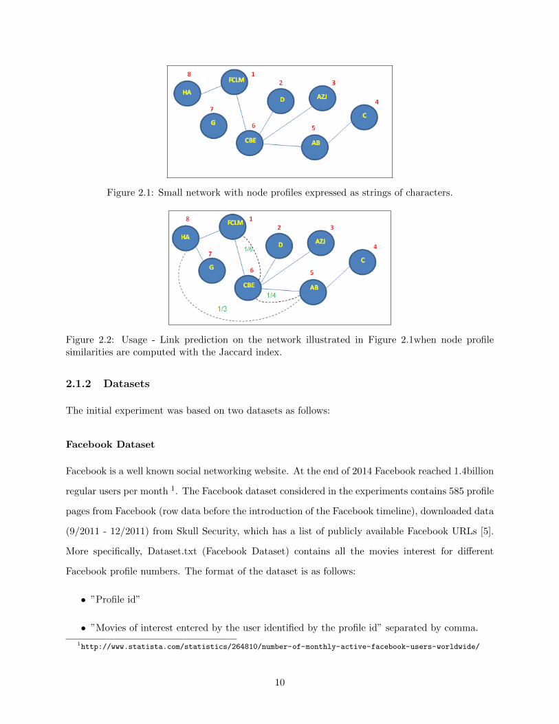
Figure 2.1: Small network with node profiles expressed as strings of characters.
Figure 2.2: Usage - Link prediction on the network illustrated in Figure 2.1when node profilesimilarities are computed with the Jaccard index.
2.1.2 Datasets
The initial experiment was based on two datasets as follows:
Facebook Dataset
Facebook is a well known social networking website. At the end of 2014 Facebook reached 1.4billion
regular users per month 1. The Facebook dataset considered in the experiments contains 585 profile
pages from Facebook (row data before the introduction of the Facebook timeline), downloaded data
(9/2011 - 12/2011) from Skull Security, which has a list of publicly available Facebook URLs [5].
More specifically, Dataset.txt (Facebook Dataset) contains all the movies interest for different
Facebook profile numbers. The format of the dataset is as follows:
• ”Profile id”
• ”Movies of interest entered by the user identified by the profile id” separated by comma.
1http://www.statista.com/statistics/264810/number-of-monthly-active-facebook-users-worldwide/
10
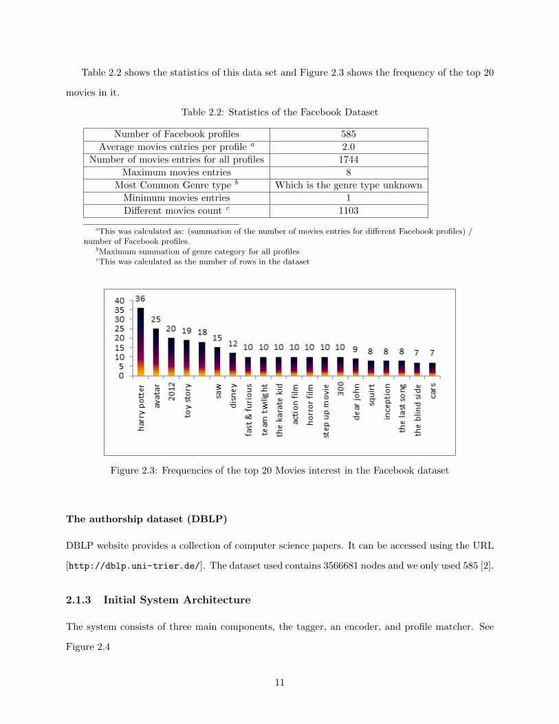
Table 2.2 shows the statistics of this data set and Figure 2.3 shows the frequency of the top 20
movies in it.
Table 2.2: Statistics of the Facebook Dataset
Number of Facebook profiles 585
Average movies entries per profile a 2.0
Number of movies entries for all profiles 1744
Maximum movies entries 8
Most Common Genre type b Which is the genre type unknown
Minimum movies entries 1
Different movies count c 1103
aThis was calculated as: (summation of the number of movies entries for different Facebook profiles) /number of Facebook profiles.
bMaximum summation of genre category for all profilescThis was calculated as the number of rows in the dataset
Figure 2.3: Frequencies of the top 20 Movies interest in the Facebook dataset
The authorship dataset (DBLP)
DBLP website provides a collection of computer science papers. It can be accessed using the URL
[http://dblp.uni-trier.de/]. The dataset used contains 3566681 nodes and we only used 585 [2].
2.1.3 Initial System Architecture
The system consists of three main components, the tagger, an encoder, and profile matcher. See
Figure 2.4
11
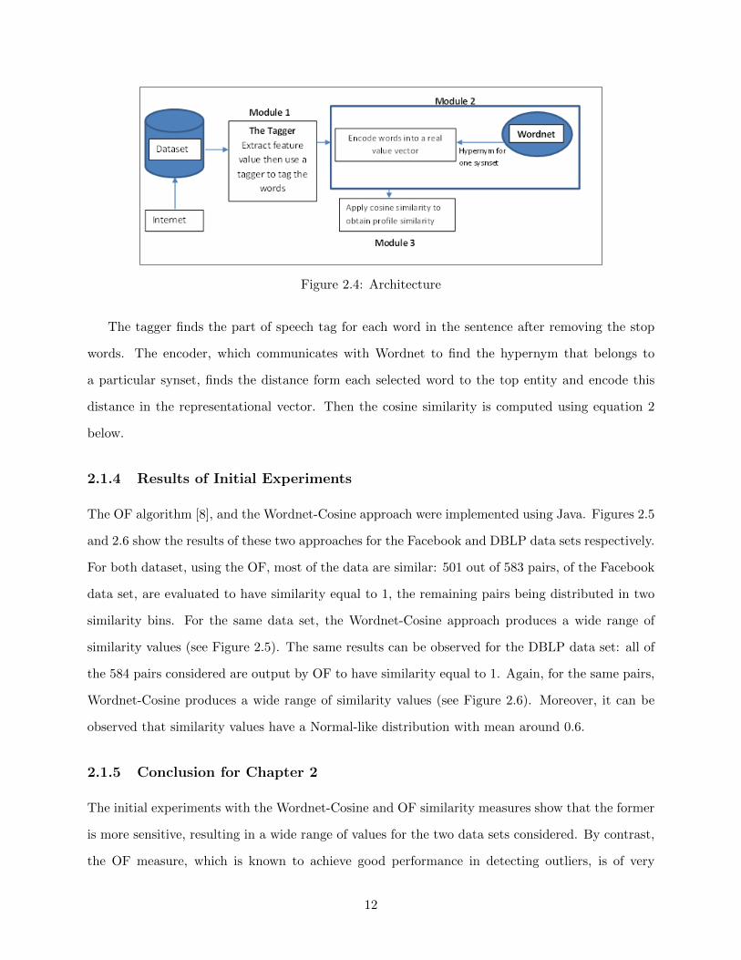
Figure 2.4: Architecture
The tagger finds the part of speech tag for each word in the sentence after removing the stop
words. The encoder, which communicates with Wordnet to find the hypernym that belongs to
a particular synset, finds the distance form each selected word to the top entity and encode this
distance in the representational vector. Then the cosine similarity is computed using equation 2
below.
2.1.4 Results of Initial Experiments
The OF algorithm [8], and the Wordnet-Cosine approach were implemented using Java. Figures 2.5
and 2.6 show the results of these two approaches for the Facebook and DBLP data sets respectively.
For both dataset, using the OF, most of the data are similar: 501 out of 583 pairs, of the Facebook
data set, are evaluated to have similarity equal to 1, the remaining pairs being distributed in two
similarity bins. For the same data set, the Wordnet-Cosine approach produces a wide range of
similarity values (see Figure 2.5). The same results can be observed for the DBLP data set: all of
the 584 pairs considered are output by OF to have similarity equal to 1. Again, for the same pairs,
Wordnet-Cosine produces a wide range of similarity values (see Figure 2.6). Moreover, it can be
observed that similarity values have a Normal-like distribution with mean around 0.6.
2.1.5 Conclusion for Chapter 2
The initial experiments with the Wordnet-Cosine and OF similarity measures show that the former
is more sensitive, resulting in a wide range of values for the two data sets considered. By contrast,
the OF measure, which is known to achieve good performance in detecting outliers, is of very
12
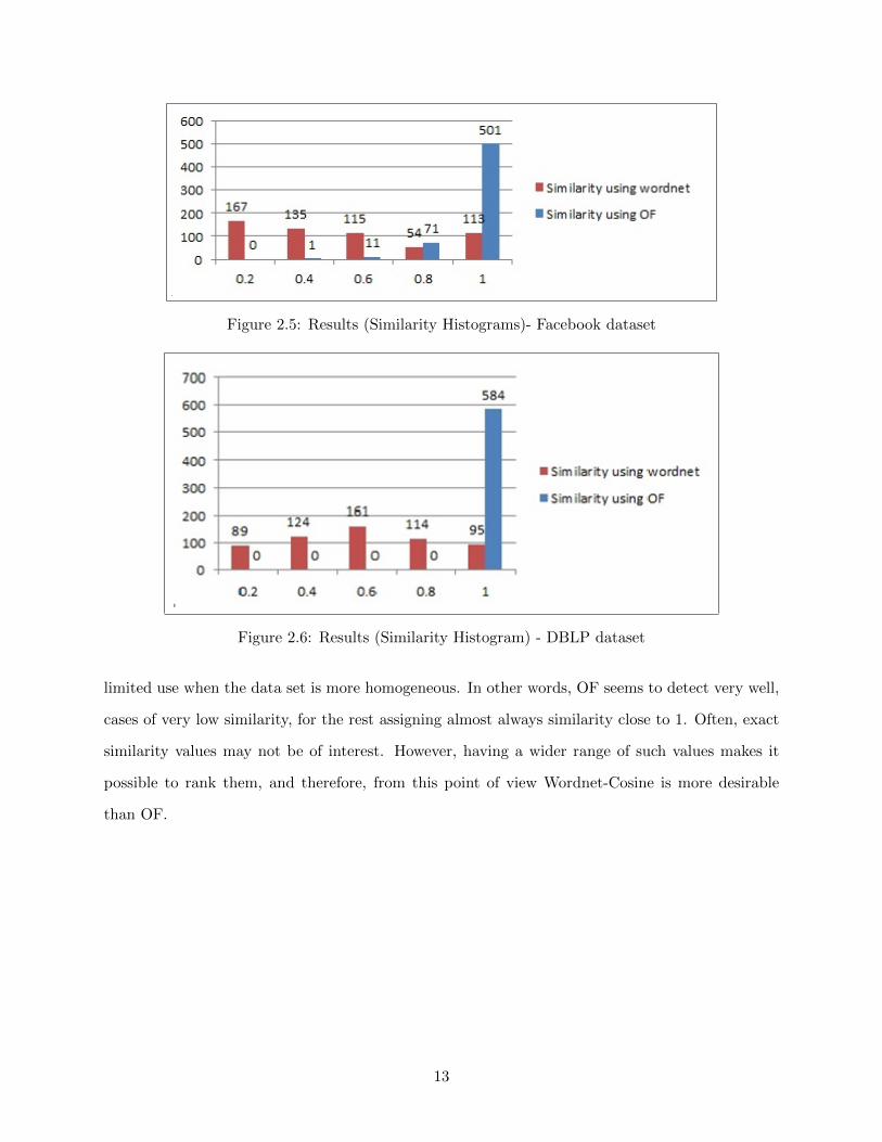
Figure 2.5: Results (Similarity Histograms)- Facebook dataset
Figure 2.6: Results (Similarity Histogram) - DBLP dataset
limited use when the data set is more homogeneous. In other words, OF seems to detect very well,
cases of very low similarity, for the rest assigning almost always similarity close to 1. Often, exact
similarity values may not be of interest. However, having a wider range of such values makes it
possible to rank them, and therefore, from this point of view Wordnet-Cosine is more desirable
than OF.
13
Chapter 3
Similarity Between Nodes in a Social
Network
14
3.1 Similarity in Social Networks
In this chapter, several similarity measures are surveyed. Finding similar nodes (node similarity) in
a social graph is the solution for many social graph problems such as link prediction, and community
formation.
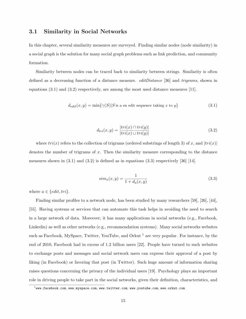
Similarity between nodes can be traced back to similarity between strings. Similarity is often
defined as a decreasing function of a distance measure. editDistance [36] and trigrams, shown in
equations (3.1) and (3.2) respectively, are among the most used distance measures [11].
dedit(x, y) = min{γ(S)|S is a en edit sequence taking x to y} (3.1)
dtri(x, y) =|tri(x) ∩ tri(y)||tri(x) ∪ tri(y)|
(3.2)
where tri(x) refers to the collection of trigrams (ordered substrings of length 3) of x, and |tri(x)|
denotes the number of trigrams of x. Then the similarity measure corresponding to the distance
measures shown in (3.1) and (3.2) is defined as in equations (3.3) respectively [36] [14].
sima(x, y) =1
1 + da(x, y)(3.3)
where a ∈ {edit, tri}.
Finding similar profiles to a network node, has been studied by many researchers [59], [26], [44],
[55]. Having systems or services that can automate this task helps in avoiding the need to search
in a large network of data. Moreover, it has many applications in social networks (e.g., Facebook,
Linkedin) as well as other networks (e.g., recommendation systems). Many social networks websites
such as Facebook, MySpace, Twitter, YouTube, and Orkut 1 are very popular. For instance, by the
end of 2010, Facebook had in excess of 1.2 billion users [22]. People have turned to such websites
to exchange posts and messages and social network users can express their approval of a post by
liking (in Facebook) or favoring that post (in Twitter). Such huge amount of information sharing
raises questions concerning the privacy of the individual users [19]. Psychology plays an important
role in driving people to take part in the social networks, given their definition, characteristics, and
1www.facebook.com, www.myspace.com, www.twitter.com, www.youtube.com, www.orkut.com
15
motivation to join such networks (see for example [25] and references therein).
Formally, social networks are represented as a graph of nodes and edges. Nodes represent
profiles and edges represent connections between two nodes. Similarity between nodes could be
based on either nodes attribute(textual) and/or edges/links(structure). Similarity measures in a
graph vary; some similarity measures [29] are based on the commonality between the nodes in the
graph (use the neighbors of nodes in the graph), while other similarity measures are based on link
similarity; these vary in the length of the path they consider [31]. For example, the link similarity
described in [31] considers paths of length greater than 2 path of length exactly 2. Others define
the link similarity based on the number of paths of varying length between such nodes [45].
Lexical database or ontologies, such as Wordnet and SNOMED CT 2 [39] and [50], may be used
in finding the similarity between items expressed as free text or keywords. Wordnet is considered
more general than the SNOMED CT ontology which is mainly in the health care domain. Moreover,
the work described in [50] finds the similarity between sentences not just words, so tools of natural
language processing (NLP), such as a tagger, are included.
Several similarity measures have been introduced including, Jaccard (biology) [28], cosine, min
[31], Sorensen, Adamic Adar [7], and resource allocation [61]; PageSim, a method to measure the
similarity between web documents was proposed in [37], based on PageRank score propagation.
PageSim was evaluated against standard information retrieval similarities TF/IDF, which were
considered to be the ground truth. Most of the similarity measures described in the literature are
knowledge dependent. However, the authors in [36] describe a knowledge independent definition
of similarity in terms of information theory. A list of similarity properties (axioms) was included
in [15].
3.2 Semantic Similarity
Using Wordnet or more special lexical database in finding similarity has been researched in many
papers [34], [27]. Different types of semantic similarity exist including
1. feature based
2. information content (which is based on the frequency of words in the dataset)
2wordnet.princeton.edu, http://www.ihtsdo.org/snomed-ct
16
3. a combination of both (hybrid)
4. ontological measures (which take into consideration the number of nodes/edgeds between two
concepts) [20].
The feature based semantic similarity uses the glossary for each concept (term) given by Word-
net. Each concept in Wordnet, is defined and thus this definition can be considered to find the
similarity in what is known as feature similarity. The path similarity uses the structural relation-
ship between the concept (taxonomy, or ontological hierarchy). Edge counting measures suffer from
irregularities in path lengths so extra attention must be taken when using them.
The information content similarity relies on the distribution of the concepts in the dataset. In
particular, it combines statistics and taxonomy structure [30]. The performance of Information
Content similarity measures is better than the measures which are only edge based as it has been
reported in [30]. Moreover, research that uses Wordnet mainly only considers the is-a relationship
(hyponymy/hypernymy) [32].
The reader can refer to [49] for further comparisons between the three similarity measures. The
authors have indicated that measures which are based on corpora statistics (information content)
require intensive computations, and therefore are impractical when the corpora is very large.
Wordnet is a free lexical database that organizes English words into concepts and relations
between them. English words, whether they are nouns, verbs, adjectives, or adverbs, are represented
as a hierarchy of synsets that are connected by a relationship between them. On the other hand,
each concept in Wordnet can have more than one synset, which is determined by the hypernym
(is-a) hierarchy.
Wordnet-Similarity, is a A Perl package that uses Wordnet to find the similarity between con-
cepts [47]. The developers of the package included the implementation of three information content
similarity measures and three edge based similarity measures.
Two research studies, that use ontology in conjunction with cosine similarity, are detailed in [39]
and [50]. However, the main difference between the two is basically in the type of ontology that has
been used ( [39] uses Wordnet while [50] uses SNOMED CT). The second difference comes from
the type of operands for the similarity measure: free text or merely keywords. The work described
in [50] uses tools of Natural Language Processing, more specifically it uses the Stanford Tagger [3].
17
3.3 Problem description and evaluation metrics
The problem of similarity can be precisely described as follows. Given a graph representation
of a social network, with two kinds of information - node attributes and link structure - find all
pairs of similar nodes based either on node profiles (node attribute) or link (structural attributes).
More formally, given a graph G = (V,E), where V, the set of vertices which represents nodes,
and E the set of edges which represents the links in the network, find all pair of similar vertices
(vi, vj), vi, vj ∈ V using the features of vi and vj or the links ei1, . . . , ein and ej1, . . . , ejm for both
the vertices vi and vj .
Each node vi in the graph can be described using a set of values for each attribute fi such that
fi ∈ F , where F is the set of all attributes of each node. Alternatively, such nodes can be also
described as having a link ei to a particular node in the graph.
The output of the similarity system is a value which represents the similarity between each
pair of nodes in the graph. The exact values of these similarities differ depending on the type of
similarity measure being used. In general, of interest is the ranking of similarity evaluations, not
their exact values.
3.4 Motivation for finding similarity
Finding the similarity between objects can be used to solve many kinds of problems: items or friends
recommendation based on the commonality [60], problems in clustering, collaborative filtering, and
search engines [23]. Different similarity measures have been used in biology, ethnology, taxonomy,
image retrieval, geology and chemistry [17], as well as in the biomedical field [39]. Neighborhood
search, centrality analysis, link prediction, graph clustering, multimedia captioning, related pages
suggestion in search engines, identifying web communities, friends suggestion in friendship network
(Facebook or MySpace), movies suggestion, item recommendation in retail service, scientific and
web domains in general, are all different kinds of applications for similarity measures in data.
An example of using similarity for clustering is collaborative filtering [23]. Zhou, Cheng and Yu
proposed an algorithm to clustering objects using attributes and structure where the attribute of
a node and the structure are independent [63]. Moreover, finding similarity between objects was
also investigated in information retrieval [37].
18
3.5 Node and other similarity measurements
Similarity in network can be based on different elements depending on the type of results that are
being sought and the type of information available. For instance, Node and edge similarities come
into presence when the graph structure is considered. On the other hand, general ontologies or
domain knowledge can be used when semantic similarities are considered. Furthermore, similarity
between words, documents, or between profiles (nodes) are used [55], [43]. Similarity measures
used in clustering [63] vary according to whether they are content-based, title-based, or keyword-
based [58].
Structure similarity (link-based). As the name implies, the structure similarity examines the
graph (links). These links may represent friendship, co-authorship, payment, etc. It has
been reported that, when compared with the human judgment, structure similarity produces
better results [33]. Such a similarity measure, based on node neighbors is described in [31].
Content similarity (text-based). As opposed to structural similarity, content similarity con-
sider the node data in finding the similarity. There are so many kinds of attributes that
can be associated with nodes such as: birth date, college, hobbies, movies interest, and age.
Crowd-sourcing can be used to collect vast number of tags that represent content such as
movies which can also be considered as a type of user-defined tags. These tags can be used
to build a new recommender system [48].
Keyword similarity (word-based). A selected subset of the possible words, known as keywords
that can occur in the node attributes may be used to find nodes similarity. An example of a
keyword similarity is the forest model described in [13], in which the keywords are organized
into a forest model, on which Wordnet is used subsequently to find the similarity between
keywords.
Table 3.1 shows a snapshot of the Facebook dataset (see Section 2.1.2 for more details about the
dataset) combined with synthetic Friends id’s data which was randomly made just for the sake of
explanation of the node and edge similarities. Each profile is represented as a set of movies interest
and a set of Facebook friends id’s. Profile similarity between these two nodes must be made in
terms of the list of movies in each of these profiles.
19
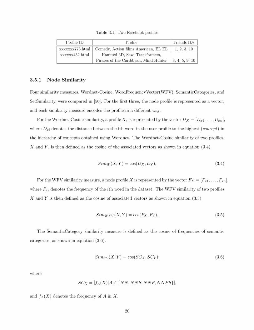
Table 3.1: Two Facebook profiles
Profile ID Profile Friends IDs
xxxxxxx773.html Comedy, Action films American, EL EL 1, 2, 3, 10
xxxxxx432.html Haunted 3D, Saw, Transformers,
Pirates of the Caribbean, Mind Hunter 3, 4, 5, 9, 10
3.5.1 Node Similarity
Four similarity measures, Wordnet-Cosine, WordFrequencyVector(WFV), SemanticCategories, and
SetSimilarity, were compared in [50]. For the first three, the node profile is represented as a vector,
and each similarity measure encodes the profile in a different way.
For the Wordnet-Cosine similarity, a profileX, is represented by the vectorDX = [Dx1, . . . , Dxn],
where Dxi denotes the distance between the ith word in the user profile to the highest (concept) in
the hierarchy of concepts obtained using Wordnet. The Wordnet-Cosine similarity of two profiles,
X and Y , is then defined as the cosine of the associated vectors as shown in equation (3.4).
SimW (X,Y ) = cos(DX , DY ), (3.4)
For the WFV similarity measure, a node profileX is represented by the vector FX = [Fx1, . . . , Fxn],
where Fxi denotes the frequency of the ith word in the dataset. The WFV similarity of two profiles
X and Y is then defined as the cosine of associated vectors as shown in equation (3.5)
SimWFV (X,Y ) = cos(FX , FY ), (3.5)
The SemanticCategory similarity measure is defined as the cosine of frequencies of semantic
categories, as shown in equation (3.6).
SimSC(X,Y ) = cos(SCX , SCY ), (3.6)
where
SCX = [fA(X)|A ∈ {NN,NNS,NNP,NNPS}],
and fA(X) denotes the frequency of A in X.
20
Finally, the SetSimilarity is defined on the basis of the sets of parents of the words in the profies,
as shown in equation (3.7).
SimS(X,Y ) =|SX ∩ SY ||SX ∪ SY |
, (3.7)
where SX = {Sxi|i = 1, . . . , n} is the set of parents for the ith word in the user profile X obtained
by using Wordnet.
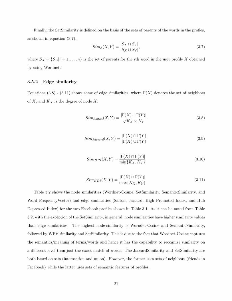
3.5.2 Edge similarity
Equations (3.8) - (3.11) shows some of edge similarities, where Γ(X) denotes the set of neighbors
of X, and KX is the degree of node X:
SimSalton(X,Y ) =|Γ(X) ∩ Γ(Y )|√
KX ×KY(3.8)
SimJaccard(X,Y ) =|Γ(X) ∩ Γ(Y )||Γ(X) ∪ Γ(Y )|
(3.9)
SimHPI(X,Y ) =|Γ(X) ∩ Γ(Y )|min{KX ,KY }
(3.10)
SimHDI(X,Y ) =|Γ(X) ∩ Γ(Y )|max{KX ,KY }
(3.11)
Table 3.2 shows the node similarities (Wordnet-Cosine, SetSimilarity, SemanticSimilarity, and
Word FrequencyVector) and edge similarities (Salton, Jaccard, High Promoted Index, and Hub
Depressed Index) for the two Facebook profiles shown in Table 3.1. As it can be noted from Table
3.2, with the exception of the SetSimilarity, in general, node similarities have higher similarity values
than edge similarities. The highest node-similarity is Worndet-Cosine and SemanticSimilarity,
followed by WFV similarity and SetSimilarity. This is due to the fact that Wordnet-Cosine captures
the semantics/meaning of terms/words and hence it has the capability to recognize similarity on
a different level than just the exact match of words. The JaccardSimilarity and SetSimilarity are
both based on sets (intersection and union). However, the former uses sets of neighbors (friends in
Facebook) while the latter uses sets of semantic features of profiles.
21
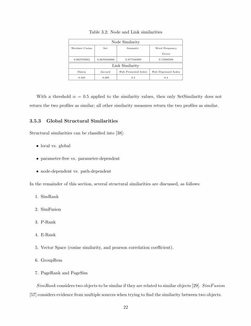
Table 3.2: Node and Link similarities
Node Similarity
Wordnet Cosine Set Semantic Word Frequency
Vector
0.862795963 0.0659340066 0.877526909 0.74900588
Link Similarity
Slaton Jaccard Hub Promoted Index Hub Depressed Index
0.423 0.285 0.5 0.4
With a threshold α = 0.5 applied to the similarity values, then only SetSimilarity does not
return the two profiles as similar; all other similarity measures return the two profiles as similar.
3.5.3 Global Structural Similarities
Structural similarities can be classified into [38]:
• local vs. global
• parameter-free vs. parameter-dependent
• node-dependent vs. path-dependent
In the remainder of this section, several structural similarities are discussed, as follows:
1. SimRank
2. SimFusion
3. P-Rank
4. E-Rank
5. Vector Space (cosine similarity, and pearson correlation coefficient).
6. GroupRem
7. PageRank and PageSim
SimRank considers two objects to be similar if they are related to similar objects [29]. SimFusion
[57] considers evidence from multiple sources when trying to find the similarity between two objects.
22
One of the differences between SimRank and SimFusion is that SimFusion uses two a random
walker approach [57]. SimRank considers two entities to be similar if they are both referenced
by similar entities. P − Rank [62] considers both in-links and out-links in contrary to SimRank.
On the other hand, E − rank considers entities to be similar if also they reference similar entities.
SetSimilarity fails to recognize similarity between objects which are represented in a hierarchical
manner, and it results in 0 similarity value between objects of different heights even though they
may be similar.
Two of the vector based similarity measures are cosine similarity and pearson correlation coef-
ficient. A comparison between six different similarity measures, including cosine index and pearson
correlation coefficient, is detailed in [61].
GroupRem is a group-based similarity measure computed on movies tags and popularity [48].
Several binary similarities between binary vectors were described in [17].
PageSim finds the similarity of web pages in search engine or web document classification. It
was inspired by PageRank, and it was evaluated against Cosine TF/IDF [37].
The ”People you may know”, friends recommender in Facebook, is based on the friends of friends
(path of length two). Several friend recommender systems have been described and compared using
precision and recall [55], [45].
3.5.4 Conclusion for Chapter 3
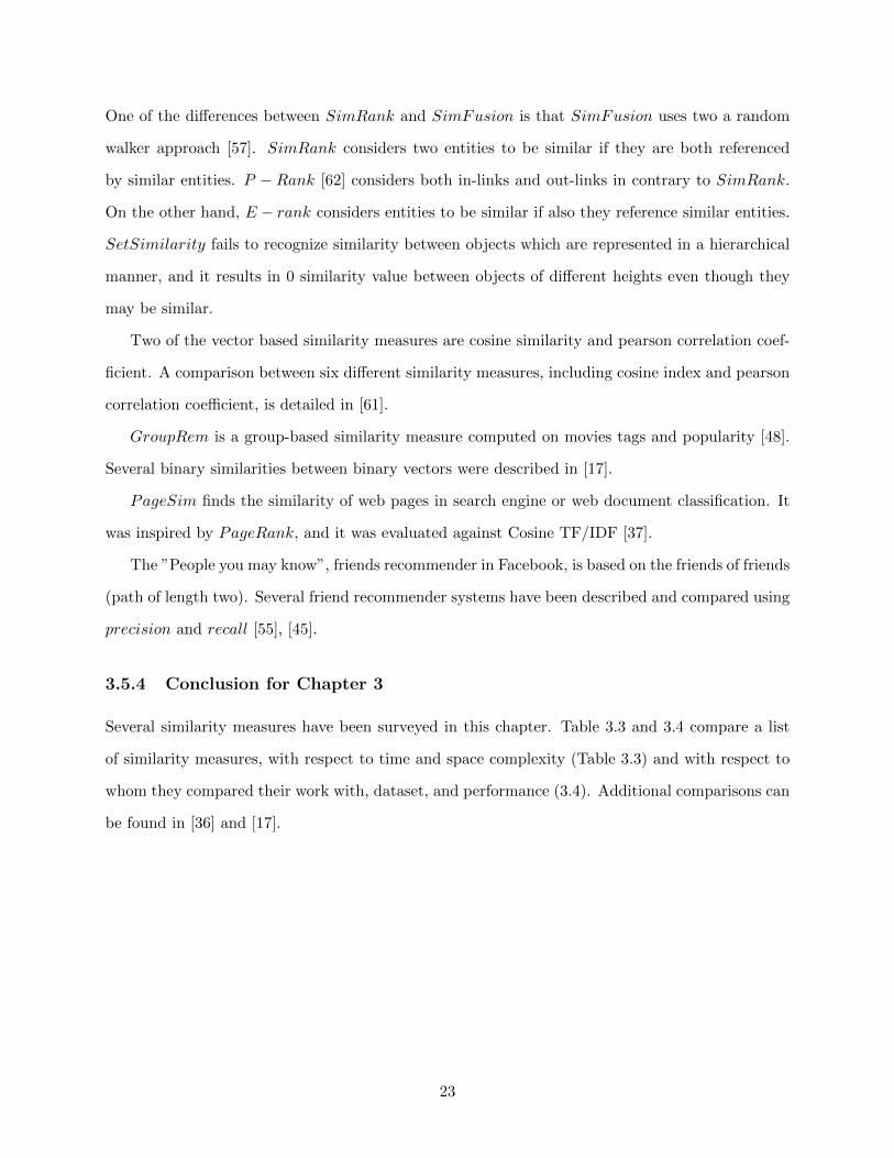
Several similarity measures have been surveyed in this chapter. Table 3.3 and 3.4 compare a list
of similarity measures, with respect to time and space complexity (Table 3.3) and with respect to
whom they compared their work with, dataset, and performance (3.4). Additional comparisons can
be found in [36] and [17].
23
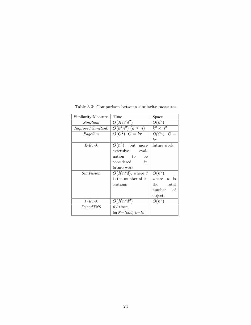
Table 3.3: Comparison between similarity measures
Similarity Measure Time Space
SimRank O(Kn2d2) O(n2)
Improved SimRank O(k4n2) (k ≤ n) k2 × n2PageSim O(C2), C = kr O(Cn), C =
kr
E-Rank O(n3), but more
extensive eval-
uation to be
considered in
future work
future work
SimFusion O(Kn2d), where d
is the number of it-
erations
O(n2),where n is
the total
number of
objects
P-Rank O(Kn2d2) O(n2)
FriendTNS 0.012sec,
forN=1000, k=10
24
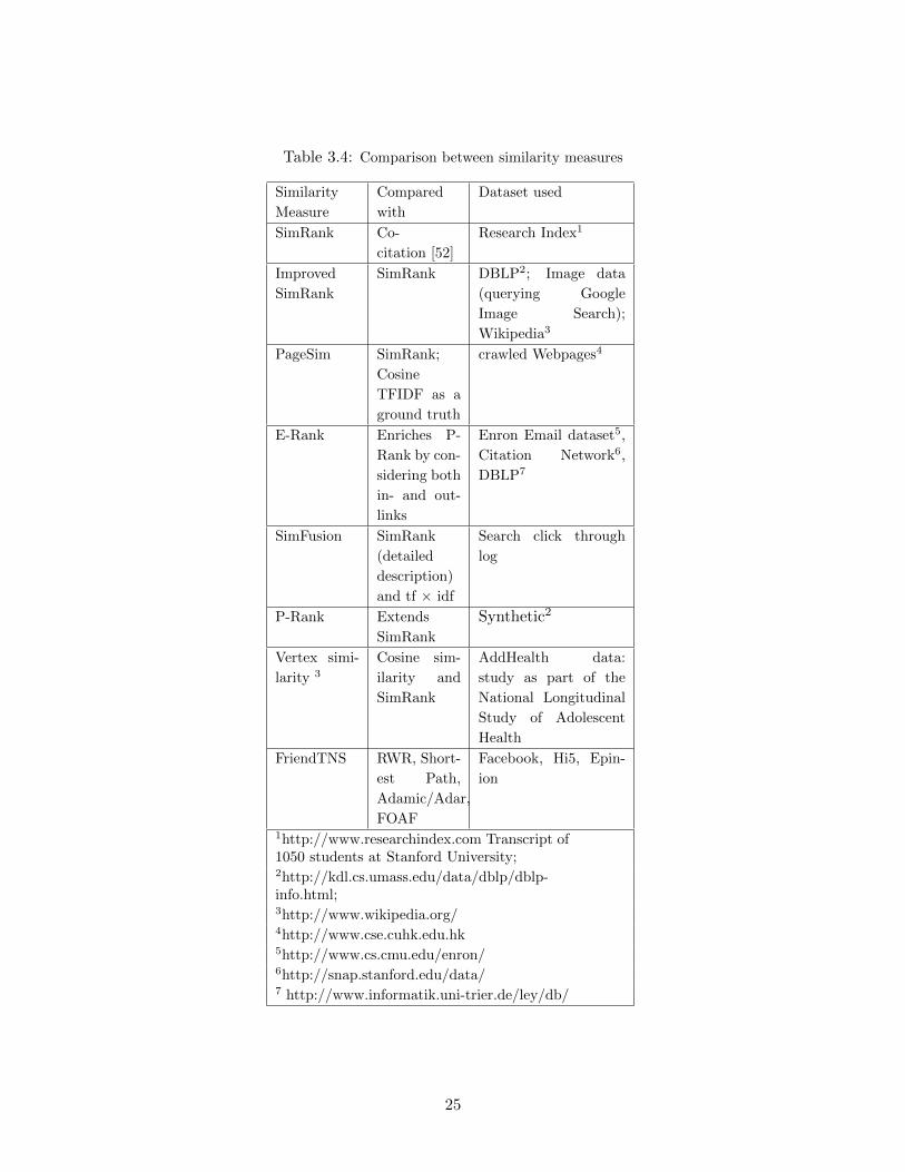
Table 3.4: Comparison between similarity measures
Similarity
Measure
Compared
with
Dataset used
SimRank Co-
citation [52]
Research Index1
Improved
SimRank
SimRank DBLP2; Image data
(querying Google
Image Search);
Wikipedia3
PageSim SimRank;
Cosine
TFIDF as a
ground truth
crawled Webpages4
E-Rank Enriches P-
Rank by con-
sidering both
in- and out-
links
Enron Email dataset5,
Citation Network6,
DBLP7
SimFusion SimRank
(detailed
description)
and tf × idf
Search click through
log
P-Rank Extends
SimRank
Synthetic2
Vertex simi-
larity 3
Cosine sim-
ilarity and
SimRank
AddHealth data:
study as part of the
National Longitudinal
Study of Adolescent
Health
FriendTNS RWR, Short-
est Path,
Adamic/Adar,
FOAF
Facebook, Hi5, Epin-
ion
1http://www.researchindex.com Transcript of1050 students at Stanford University;2http://kdl.cs.umass.edu/data/dblp/dblp-info.html;3http://www.wikipedia.org/4http://www.cse.cuhk.edu.hk5http://www.cs.cmu.edu/enron/6http://snap.stanford.edu/data/7 http://www.informatik.uni-trier.de/ley/db/
25
Chapter 4
Semantic Similiarity Measures
26
4.1 Similarity measures and Semantic
As it has been mentioned earlier, several similarity measures have been developed and they can be
used in various applications. lexical database, such as Wordnet, can be used to assist in obtaining
the semantic underlying the content of the node profile in networks. Such semantic content, can
be used in calculating the similarity between the data. In this chapter, more about the semantic
analysis (using Wordnet), and how it can be integrated into the proposed similarity measure,
Wordnet-Cosine, is described.
4.2 Finding Similar Profiles
4.2.1 Wordnet
As already mentioned the current approach makes use of Wordnet, a free lexical database that
organizes English words into concepts and relations, well-known for assessing semantic similarity.
This section discusses in more detail the elements of Wordnet. English nouns, verbs, adjectives,
and adverbs form hierarchies of synset where relations exist that connect them. Of the six relations
defined in Wordnet, Synonymy, Antonymy, Hypernymy, Meronymy, Troponymy, Entailment, this
study uses only Hypernymy.
Hypernym of a word
Informally, Hypernym of a word is its super class concept. It is equivalent to the is-a or kind-of
relationships used in ontologies. The opposite of Hypernym is Hyponym which is the sub-class.
Consider for example, the two senses of word ”comedy”:
• comedy as a ”humorous drama”
• comedy as ”comic incident”
For the first sense, comedy is a kind of drama, which is a kind of literary work. Therefore, literary
work is a hypernym of drama, and drama is a hypernym of comedy [41]. The hierarchy determined
by the hypernym relationship is called a synset. Therefore, based on the above, the synset for
27
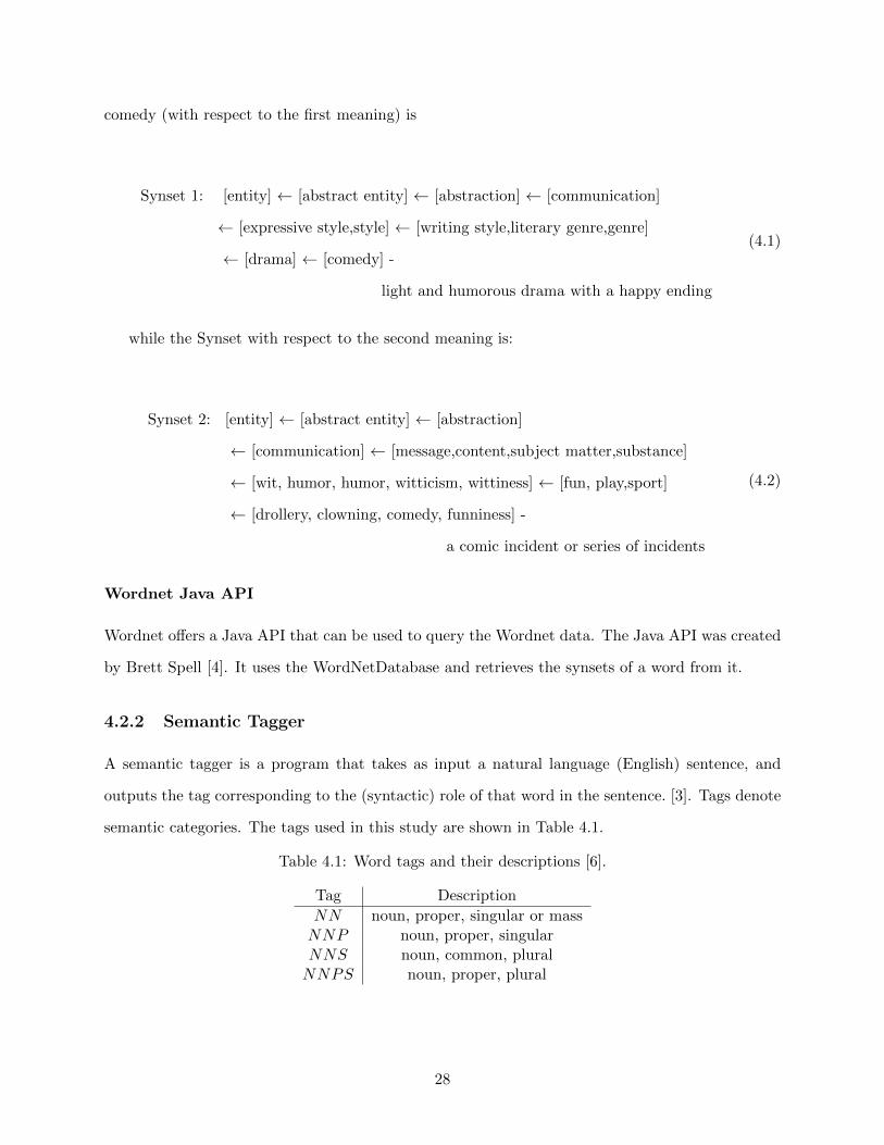
comedy (with respect to the first meaning) is
Synset 1: [entity] ← [abstract entity] ← [abstraction] ← [communication]
← [expressive style,style] ← [writing style,literary genre,genre]
← [drama] ← [comedy] -
light and humorous drama with a happy ending
(4.1)
while the Synset with respect to the second meaning is:
Synset 2: [entity] ← [abstract entity] ← [abstraction]
← [communication] ← [message,content,subject matter,substance]
← [wit, humor, humor, witticism, wittiness] ← [fun, play,sport]
← [drollery, clowning, comedy, funniness] -
a comic incident or series of incidents
(4.2)
Wordnet Java API
Wordnet offers a Java API that can be used to query the Wordnet data. The Java API was created
by Brett Spell [4]. It uses the WordNetDatabase and retrieves the synsets of a word from it.
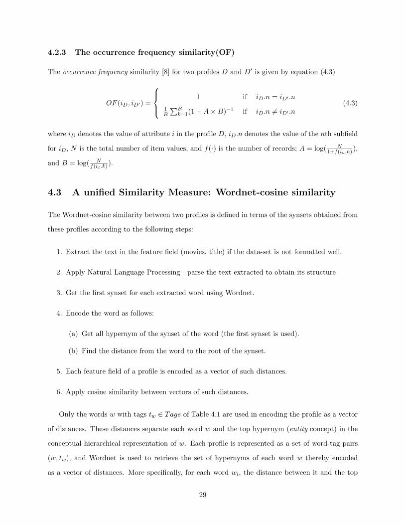
4.2.2 Semantic Tagger
A semantic tagger is a program that takes as input a natural language (English) sentence, and
outputs the tag corresponding to the (syntactic) role of that word in the sentence. [3]. Tags denote
semantic categories. The tags used in this study are shown in Table 4.1.
Table 4.1: Word tags and their descriptions [6].
Tag Description
NN noun, proper, singular or massNNP noun, proper, singularNNS noun, common, pluralNNPS noun, proper, plural
28
4.2.3 The occurrence frequency similarity(OF)
The occurrence frequency similarity [8] for two profiles D and D′ is given by equation (4.3)
OF (iD, iD′) =
1 if iD.n = iD′ .n
1B
∑Bk=1(1 +A×B)−1 if iD.n 6= iD′ .n
(4.3)
where iD denotes the value of attribute i in the profile D, iD.n denotes the value of the nth subfield
for iD, N is the total number of item values, and f(·) is the number of records; A = log( N1+f(iu.n)
),
and B = log( Nf(ix.k)
).
4.3 A unified Similarity Measure: Wordnet-cosine similarity
The Wordnet-cosine similarity between two profiles is defined in terms of the synsets obtained from
these profiles according to the following steps:
1. Extract the text in the feature field (movies, title) if the data-set is not formatted well.
2. Apply Natural Language Processing - parse the text extracted to obtain its structure
3. Get the first synset for each extracted word using Wordnet.
4. Encode the word as follows:
(a) Get all hypernym of the synset of the word (the first synset is used).
(b) Find the distance from the word to the root of the synset.
5. Each feature field of a profile is encoded as a vector of such distances.
6. Apply cosine similarity between vectors of such distances.
Only the words w with tags tw ∈ Tags of Table 4.1 are used in encoding the profile as a vector
of distances. These distances separate each word w and the top hypernym (entity concept) in the
conceptual hierarchical representation of w. Each profile is represented as a set of word-tag pairs
(w, tw), and Wordnet is used to retrieve the set of hypernyms of each word w thereby encoded
as a vector of distances. More specifically, for each word wi, the distance between it and the top
29
hypernym is found and placed as the ith component value of the vector representing the profile.
The distance di = d(wi) for each given word is computed according to equation (4.4)
d(w) =
dist(w, [entity]) if w is in Wordnet
0 otherwise(4.4)
For example, given the word “comedy”, whose tag, NN , belongs to Tags of Table 4.1, its
encoding will be the distance between it and the entity concept, and this distance is equal to 7.
For words that don’t have any hypyernym, their encoding is 0. Words that have a tag 6∈ Tags of
Table 4.1 are ignored.
The encoding of a profile D is a mapping e : D 7→ <k+ such that
e(D) = (d1, . . . , dk)
The Wordnet-Cosine similarity between D and D′, where D and D′ are two profiles with encodings
e(D) = (d1, . . . , dk) and e(D′) = (d′1, . . . , d′k), is given by the cosine similarity between the encoding
e(D) and e(D′) of the two profiles, shown in equation (4.5).
Sim(D,D′) = cos(e(D), e(D′)) =e(D) · e(D′)‖e(D)‖‖e(D′)‖
(4.5)
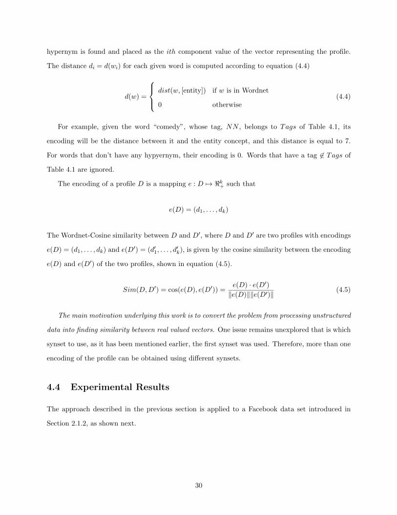
The main motivation underlying this work is to convert the problem from processing unstructured
data into finding similarity between real valued vectors. One issue remains unexplored that is which
synset to use, as it has been mentioned earlier, the first synset was used. Therefore, more than one
encoding of the profile can be obtained using different synsets.
4.4 Experimental Results
The approach described in the previous section is applied to a Facebook data set introduced in
Section 2.1.2, as shown next.
30
4.4.1 Facebook profiles data-set
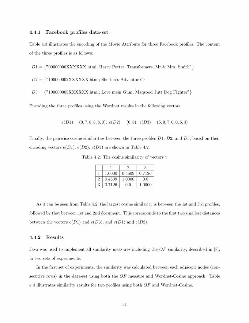
Table 4.3 illustrates the encoding of the Movie Attribute for three Facebook profiles. The content
of the three profiles is as follows:
D1 = {”00000000XXXXXX.html; Harry Potter, Transformers, Mr.& Mrs. Smith”}
D2 = {”100000002XXXXXX.html; Sherina’s Adventure”}
D3 = {”100000005XXXXXX.html; Love mein Gum, Maqsood Jutt Dog Fighter”}
Encoding the three profiles using the Wordnet results in the following vectors:
e(D1) = (0, 7, 8, 8, 8, 0); e(D2) = (0, 8); e(D3) = (5, 0, 7, 0, 0, 6, 4)
Finally, the pairwise cosine similarities between the three profiles D1, D2, and D3, based on their
encoding vectors e(D1), e(D2), e(D3) are shown in Table 4.2.
Table 4.2: The cosine similarity of vectors v
1 2 3
1 1.0000 0.4509 0.7126
2 0.4509 1.0000 0.0
3 0.7126 0.0 1.0000
As it can be seen from Table 4.2, the largest cosine similarity is between the 1st and 3rd profiles,
followed by that between 1st and 2nd document. This corresponds to the first two smallest distances
between the vectors e(D1) and e(D3), and e(D1) and e(D2).
4.4.2 Results
Java was used to implement all similarity measures including the OF similarity, described in [8],
in two sets of experiments.
In the first set of experiments, the similarity was calculated between each adjacent nodes (con-
secutive rows) in the data-set using both the OF measure and Wordnet-Cosine approach. Table
4.4 illustrates similarity results for two profiles using both OF and Wordnet-Cosine.
31
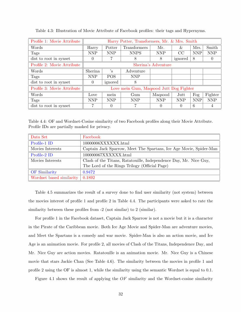
Table 4.3: Illustration of Movie Attribute of Facebook profiles: their tags and Hypernyms.
Profile 1: Movie Attribute Harry Potter, Transformers, Mr. & Mrs. Smith
Words Harry Potter Transformers Mr. & Mrs. Smith
Tags NNP NNP NNPS NNP CC NNP NNP
dist to root in synset 0 7 8 8 ignored 8 0
Profile 2: Movie Attribute Sherina’s Adventure
Words Sherina ’s Adventure
Tags NNP POS NNP
dist to root in synset 0 ignored 8
Profile 3: Movie Attribute Love mein Gum, Maqsood Jutt Dog Fighter
Words Love mein Gum Maqsood Jutt Fog Fighter
Tags NNP NNP NNP NNP NNP NNP NNP
dist to root in synset 7 0 7 0 0 6 4
Table 4.4: OF and Wordnet-Cosine similarity of two Facebook profiles along their Movie Attribute.Profile IDs are partially masked for privacy.
Data Set Facebook
Profile-1 ID 10000006XXXXXX.html
Movies Interests Captain Jack Sparrow, Meet The Spartans, Ice Age Movie, Spider-Man
Profile-2 ID 100000067XXXXXX.html
Movies Interests Clash of the Titans, Ratatouille, Independence Day, Mr. Nice Guy,The Lord of the Rings Trilogy (Official Page)
OF Similarity 0.9472
Wordnet based similarity 0.1892
Table 4.5 summarizes the result of a survey done to find user similarity (not system) between
the movies interest of profile 1 and profile 2 in Table 4.4. The participants were asked to rate the
similarity between these profiles from -2 (not similar) to 2 (similar).
For profile 1 in the Facebook dataset, Captain Jack Sparrow is not a movie but it is a character
in the Pirate of the Caribbean movie. Both Ice Age Movie and Spider-Man are adventure movies,
and Meet the Spartans is a comedy and war movie. Spider-Man is also an action movie, and Ice
Age is an animation movie. For profile 2, all movies of Clash of the Titans, Independence Day, and
Mr. Nice Guy are action movies. Ratatouille is an animation movie. Mr. Nice Guy is a Chinese
movie that stars Jackie Chan (See Table 4.6). The similarity between the movies in profile 1 and
profile 2 using the OF is almost 1, while the similarity using the semantic Wordnet is equal to 0.1.
Figure 4.1 shows the result of applying the OF similarity and the Wordnet-cosine similarity
32
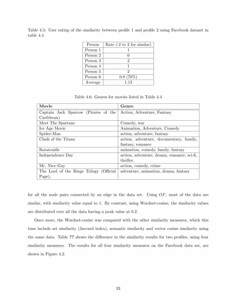
Table 4.5: User rating of the similarity between profile 1 and profile 2 using Facebook dataset intable 4.4
Person Rate (-2 to 2 for similar)
Person 1 1
Person 2 0
Person 3 2
Person 4 1
Person 5 2
Person 6 0.8 (70%)
Average 1.13
Table 4.6: Genres for movies listed in Table 4.4
Movie Genre
Captain Jack Sparrow (Pirates of theCaribbean)
Action, Adventure, Fantasy
Meet The Spartans Comedy, war
Ice Age Movie Animation, Adventure, Comedy
Spider-Man action, adventure, fantasy
Clash of the Titans action, adventure, documentary, family,fantasy, romance
Ratatouille animation, comedy, family, fantasy
Independence Day action, adventure, drama, romance, sci-fi,thriller
Mr. Nice Guy action, comedy, crime
The Lord of the Rings Trilogy (OfficialPage),
adventure, animation, drama, fantasy
for all the node pairs connected by an edge in the data set. Using OF , most of the data are
similar, with similarity value equal to 1. By contrast, using Wordnet-cosine, the similarity values
are distributed over all the data having a peak value at 0.2.
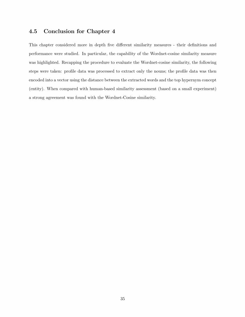
Once more, the Wordnet-cosine was compared with the other similarity measures, which this
time include set similarity (Jaccard index), semantic similarity and vector cosine similarity using
the same data. Table ?? shows the difference in the similarity results for two profiles, using four
similarity measures. The results for all four similarity measures on the Facebook data set, are
shown in Figure 4.2.
33
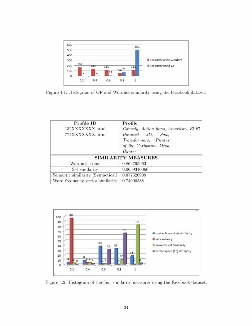
Figure 4.1: Histogram of OF and Wordnet similarity using the Facebook dataset.
Profile ID Profile132XXXXXXX.html Comedy, Action films, American, El El
774XXXXXXX.html Haunted 3D, Saw,Transformers, Piratesof the Caribbean, MindHunter
SIMILARITY MEASURES
Wordnet cosine 0.862795963
Set similarity 0.0659340066
Semantic similarity (Syntactical) 0.877526909
Word frequency vector similarity 0.74900588
Figure 4.2: Histogram of the four similarity measures using the Facebook dataset.
34
4.5 Conclusion for Chapter 4
This chapter considered more in depth five different similarity measures - their definitions and
performance were studied. In particular, the capability of the Wordnet-cosine similarity measure
was highlighted. Recapping the procedure to evaluate the Wordnet-cosine similarity, the following
steps were taken: profile data was processed to extract only the nouns; the profile data was then
encoded into a vector using the distance between the extracted words and the top hypernym concept
(entity). When compared with human-based similarity assessment (based on a small experiment)
a strong agreement was found with the Wordnet-Cosine similarity.
35
Chapter 5
Algorithms and Implementations for
Finding Similarity
5.1 Java algorithms for finding similarities
This chapter includes a description and a discussion of the similarity algorithms used. The algo-
rithms were applied on Facebook, MovieLens, or DBLP datasets. All of the similarity measures
were implemented using Java, this choice was influenced by the fact that Wordnet-cosine similarity,
the proposed similarity, uses Wordnet API (Application Programmer Interface) [4] which is written
in Java.
The code for finding each similarity measure was divided into three different types of methods.
The dependency between such methods is illustrated in figure 5.1 and 5.2. As it can be seen from
these figure, the GetResults (similarity measure) method calls find (similarity measure), which in
turn calls getDistance (similarity measure). The role of each method is as follows:
• GetResults iterates through all pairs of data (lines) in the dataset and invokes find . It writes
the similairty value between each pair of data into a text file.
• find invokes getDistance with two lines passed as arguments, and then it finds the similarity
between the its arguments, and returns this similarity to GetResults (similarity measure).
• getDistance encodes each line in the dataset as a vector according to the specification of each
similarity measure.
36
Each similarity measure encodes each line in the dataset in a distinctive manner. However, all
of the similarity measures encode each line as a vector with varying characteristics, some of which
are shared among the different similarity measures. The detailed descriptions of how each line is
encoded into a vector, based on the different similarity measures are as follows:
SetSimilarity. Each line is encoded as a set-valued vector: each component is the set ancestors
(parents) from a word in the profile, to the top entity in the conceptual hierarchy retrieved
by Wordnet.
Wordnet-Cosine similarity. The encoding is similar, to some extent, to the encoding of the
set similarity detailed in the previous item. However, each vector, which represents a profile,
is created by finding the length of the path that connects every word in the line to the entity
concept in the conceptual hierarchy retrieved by Wordnet.
Semantic Categories. Encodes each line as a vector that contains the frequency of words that
belong to the categories NN, NNS, NNP, NNPS ( so for instance, v = 2 NN, 3 NNS, 0 NNP,
0 NNPS).
Word Frequency Vector. Encoding is similar to the one made by the Semantic Categories
where each component of the vector is the frequency of the word in the profile (not the
frequency of its semantic category).
For an algorithm description of the encoding for each similarity measure, refer to the corre-
sponding algorithms 4, 7, 10, and 13 Each similarity measure uses different criteria for calculating
the similarity, and this can be summarized as follows:
Set similarity calculates the similarity between two profiles as the ratio of the size of the inter-
section of the sets representing each and the size of the union of such sets. Note: Recall that
each set contains the parent set.
Wordnet-Cosine, Semantic Categories, and Word Frequency Vector similarities are all
baseed on the cosine similarity of the corresponding vector representation.
37
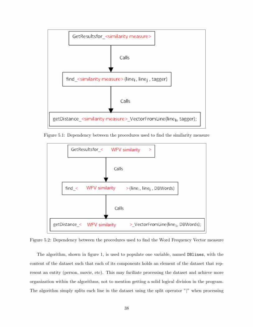
Figure 5.1: Dependency between the procedures used to find the similarity measure
Figure 5.2: Dependency between the procedures used to find the Word Frequency Vector measure
The algorithm, shown in figure 1, is used to populate one variable, named DBlines, with the
content of the dataset such that each of its components holds an element of the dataset that rep-
resent an entity (person, movie, etc). This may faciliate processing the dataset and achieve more
organization within the algorithms, not to mention getting a solid logical division in the program.
The algorithm simply splits each line in the dataset using the split operator ”|” when processing
38
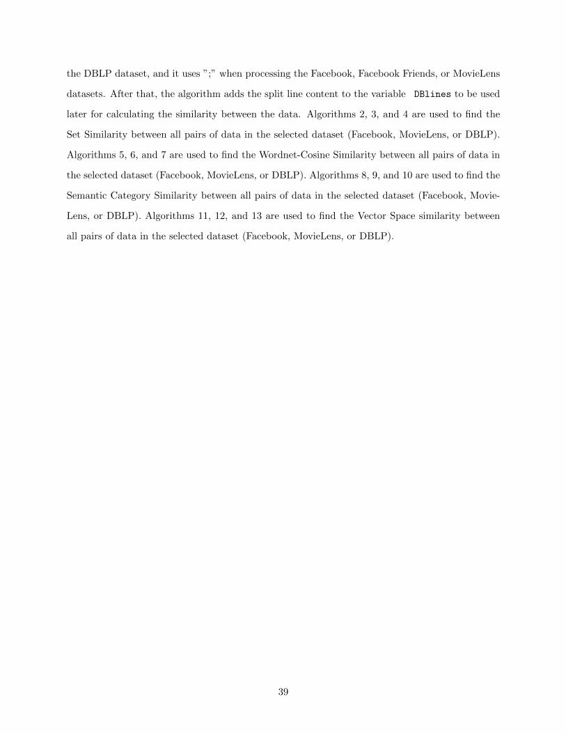
the DBLP dataset, and it uses ”;” when processing the Facebook, Facebook Friends, or MovieLens
datasets. After that, the algorithm adds the split line content to the variable DBlines to be used
later for calculating the similarity between the data. Algorithms 2, 3, and 4 are used to find the
Set Similarity between all pairs of data in the selected dataset (Facebook, MovieLens, or DBLP).
Algorithms 5, 6, and 7 are used to find the Wordnet-Cosine Similarity between all pairs of data in
the selected dataset (Facebook, MovieLens, or DBLP). Algorithms 8, 9, and 10 are used to find the
Semantic Category Similarity between all pairs of data in the selected dataset (Facebook, Movie-
Lens, or DBLP). Algorithms 11, 12, and 13 are used to find the Vector Space similarity between
all pairs of data in the selected dataset (Facebook, MovieLens, or DBLP).
39
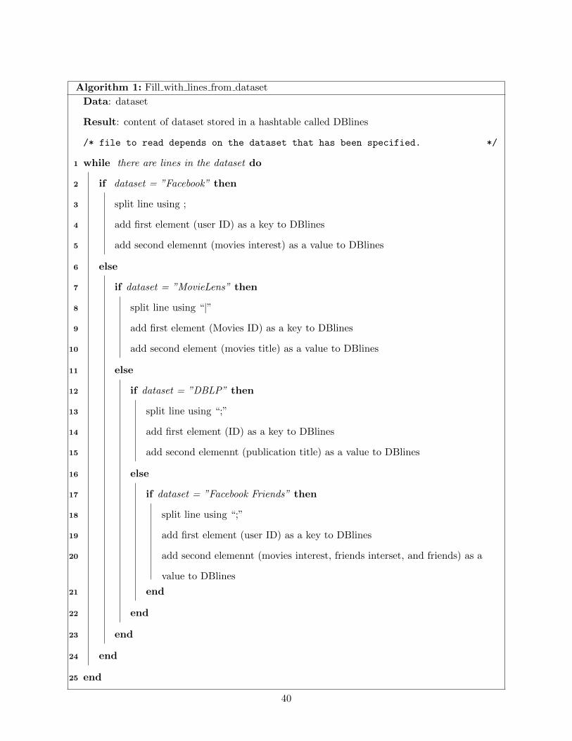
Algorithm 1: Fill with lines from dataset
Data: dataset
Result: content of dataset stored in a hashtable called DBlines
/* file to read depends on the dataset that has been specified. */
1 while there are lines in the dataset do
2 if dataset = ”Facebook” then
3 split line using ;
4 add first element (user ID) as a key to DBlines
5 add second elemennt (movies interest) as a value to DBlines
6 else
7 if dataset = ”MovieLens” then
8 split line using “|”
9 add first element (Movies ID) as a key to DBlines
10 add second element (movies title) as a value to DBlines
11 else
12 if dataset = ”DBLP” then
13 split line using “;”
14 add first element (ID) as a key to DBlines
15 add second elemennt (publication title) as a value to DBlines
16 else
17 if dataset = ”Facebook Friends” then
18 split line using “;”
19 add first element (user ID) as a key to DBlines
20 add second elemennt (movies interest, friends interset, and friends) as a
value to DBlines
21 end
22 end
23 end
24 end
25 end
40
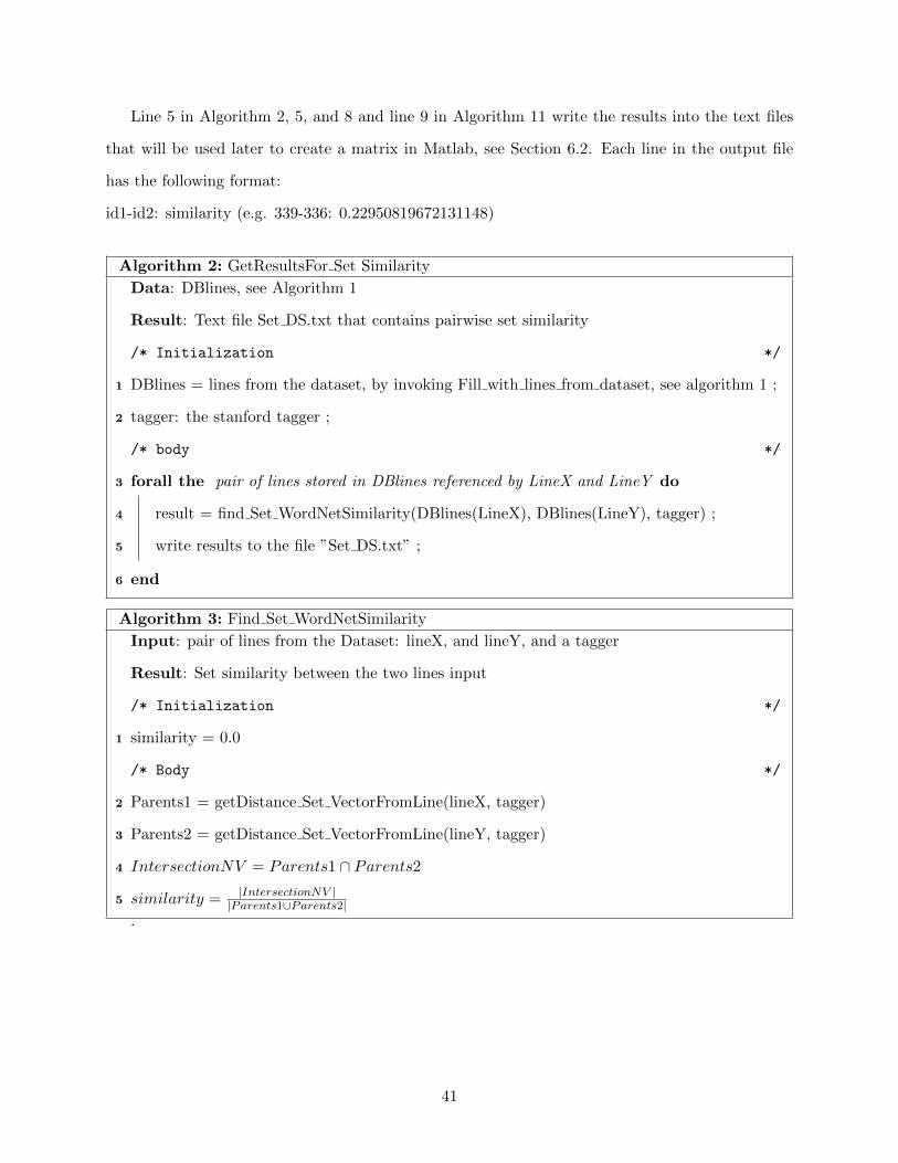
Line 5 in Algorithm 2, 5, and 8 and line 9 in Algorithm 11 write the results into the text files
that will be used later to create a matrix in Matlab, see Section 6.2. Each line in the output file
has the following format:
id1-id2: similarity (e.g. 339-336: 0.22950819672131148)
Algorithm 2: GetResultsFor Set Similarity
Data: DBlines, see Algorithm 1
Result: Text file Set DS.txt that contains pairwise set similarity
/* Initialization */
1 DBlines = lines from the dataset, by invoking Fill with lines from dataset, see algorithm 1 ;
2 tagger: the stanford tagger ;
/* body */
3 forall the pair of lines stored in DBlines referenced by LineX and LineY do
4 result = find Set WordNetSimilarity(DBlines(LineX), DBlines(LineY), tagger) ;
5 write results to the file ”Set DS.txt” ;
6 end
Algorithm 3: Find Set WordNetSimilarity
Input: pair of lines from the Dataset: lineX, and lineY, and a tagger
Result: Set similarity between the two lines input
/* Initialization */
1 similarity = 0.0
/* Body */
2 Parents1 = getDistance Set VectorFromLine(lineX, tagger)
3 Parents2 = getDistance Set VectorFromLine(lineY, tagger)
4 IntersectionNV = Parents1 ∩ Parents2
5 similarity = |IntersectionNV ||Parents1∪Parents2|
.
41
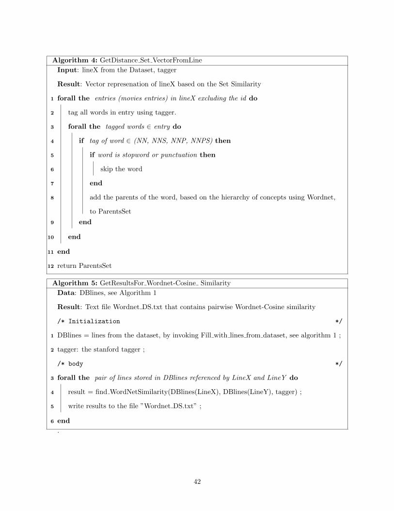
Algorithm 4: GetDistance Set VectorFromLine
Input: lineX from the Dataset, tagger
Result: Vector represenation of lineX based on the Set Similarity
1 forall the entries (movies entries) in lineX excluding the id do
2 tag all words in entry using tagger.
3 forall the tagged words ∈ entry do
4 if tag of word ∈ (NN, NNS, NNP, NNPS) then
5 if word is stopword or punctuation then
6 skip the word
7 end
8 add the parents of the word, based on the hierarchy of concepts using Wordnet,
to ParentsSet
9 end
10 end
11 end
12 return ParentsSet
Algorithm 5: GetResultsFor Wordnet-Cosine Similarity
Data: DBlines, see Algorithm 1
Result: Text file Wordnet DS.txt that contains pairwise Wordnet-Cosine similarity
/* Initialization */
1 DBlines = lines from the dataset, by invoking Fill with lines from dataset, see algorithm 1 ;
2 tagger: the stanford tagger ;
/* body */
3 forall the pair of lines stored in DBlines referenced by LineX and LineY do
4 result = find WordNetSimilarity(DBlines(LineX), DBlines(LineY), tagger) ;
5 write results to the file ”Wordnet DS.txt” ;
6 end
.
42
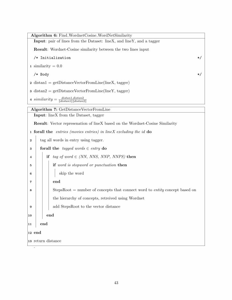
Algorithm 6: Find WordnetCosine WordNetSimilarity
Input: pair of lines from the Dataset: lineX, and lineY, and a tagger
Result: Wordnet-Cosine similarity between the two lines input
/* Initialization */
1 similarity = 0.0
/* Body */
2 distan1 = getDistanceVectorFromLine(lineX, tagger)
3 distan2 = getDistanceVectorFromLine(lineY, tagger)
4 similarity = distan1.distan2‖distan1‖‖distan2‖
Algorithm 7: GetDistanceVectorFromLine
Input: lineX from the Dataset, tagger
Result: Vector represenation of lineX based on the Wordnet-Cosine Similarity
1 forall the entries (movies entries) in lineX excluding the id do
2 tag all words in entry using tagger.
3 forall the tagged words ∈ entry do
4 if tag of word ∈ (NN, NNS, NNP, NNPS) then
5 if word is stopword or punctuation then
6 skip the word
7 end
8 StepsRoot = number of concepts that connect word to entity concept based on
the hierarchy of concepts, retreived using Wordnet
9 add StepsRoot to the vector distance
10 end
11 end
12 end
13 return distance
.
43
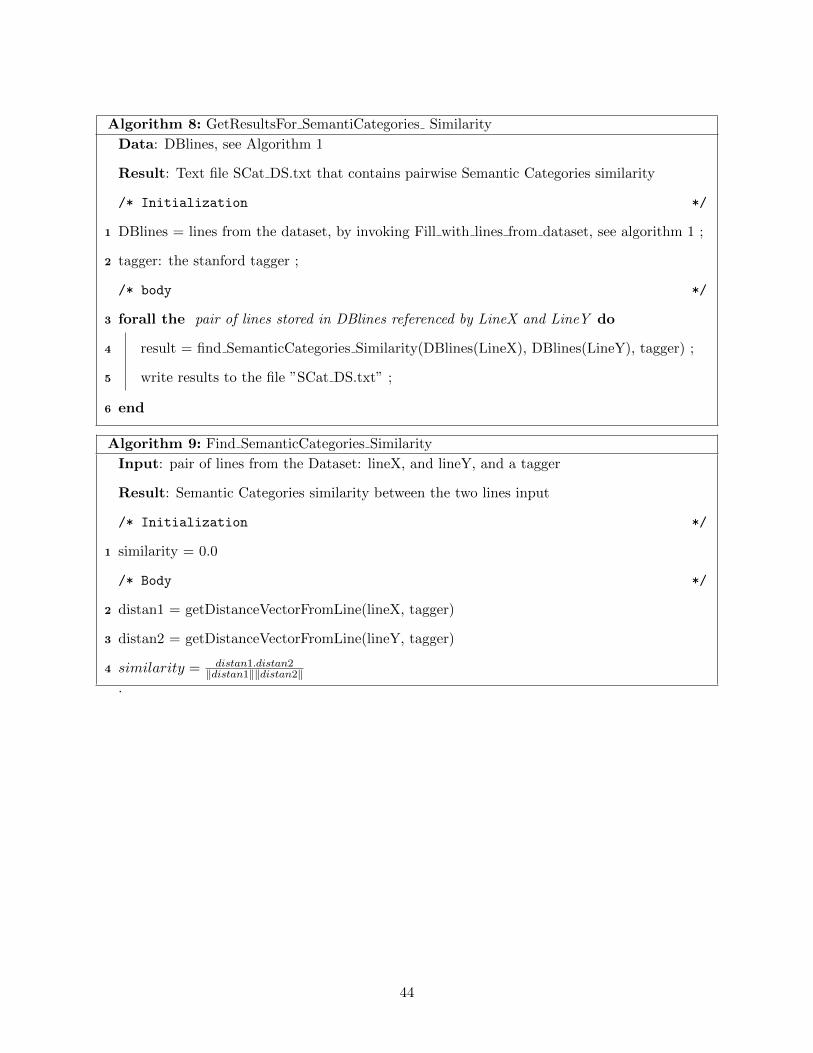
Algorithm 8: GetResultsFor SemantiCategories Similarity
Data: DBlines, see Algorithm 1
Result: Text file SCat DS.txt that contains pairwise Semantic Categories similarity
/* Initialization */
1 DBlines = lines from the dataset, by invoking Fill with lines from dataset, see algorithm 1 ;
2 tagger: the stanford tagger ;
/* body */
3 forall the pair of lines stored in DBlines referenced by LineX and LineY do
4 result = find SemanticCategories Similarity(DBlines(LineX), DBlines(LineY), tagger) ;
5 write results to the file ”SCat DS.txt” ;
6 end
Algorithm 9: Find SemanticCategories Similarity
Input: pair of lines from the Dataset: lineX, and lineY, and a tagger
Result: Semantic Categories similarity between the two lines input
/* Initialization */
1 similarity = 0.0
/* Body */
2 distan1 = getDistanceVectorFromLine(lineX, tagger)
3 distan2 = getDistanceVectorFromLine(lineY, tagger)
4 similarity = distan1.distan2‖distan1‖‖distan2‖
.
44
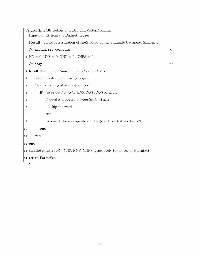
Algorithm 10: GetDistance SemCat VectorFromLine
Input: lineX from the Dataset, tagger
Result: Vector represenation of lineX based on the Semantic Categories Similarity
/* Initialize counters: */
1 NN = 0, NNS = 0, NNP = 0, NNPS = 0
/* body */
2 forall the entries (movies entries) in lineX do
3 tag all words in entry using tagger.
4 forall the tagged words ∈ entry do
5 if tag of word ∈ (NN, NNS, NNP, NNPS) then
6 if word is stopword or punctuation then
7 skip the word
8 end
9 increment the appropriate counter (e.g. NN++ if word is NN)
10 end
11 end
12 end
13 add the counters NN, NNS, NNP, NNPS respectively to the vector ParentSet.
14 return ParentSet.
.
45
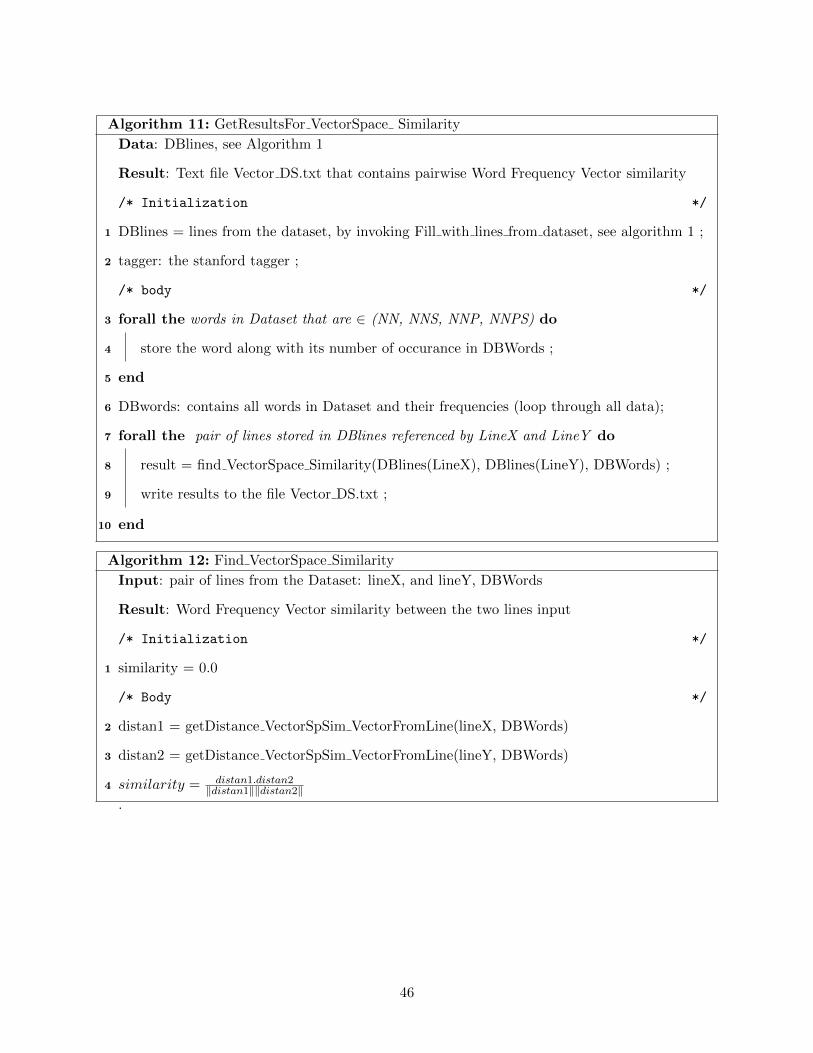
Algorithm 11: GetResultsFor VectorSpace Similarity
Data: DBlines, see Algorithm 1
Result: Text file Vector DS.txt that contains pairwise Word Frequency Vector similarity
/* Initialization */
1 DBlines = lines from the dataset, by invoking Fill with lines from dataset, see algorithm 1 ;
2 tagger: the stanford tagger ;
/* body */
3 forall the words in Dataset that are ∈ (NN, NNS, NNP, NNPS) do
4 store the word along with its number of occurance in DBWords ;
5 end
6 DBwords: contains all words in Dataset and their frequencies (loop through all data);
7 forall the pair of lines stored in DBlines referenced by LineX and LineY do
8 result = find VectorSpace Similarity(DBlines(LineX), DBlines(LineY), DBWords) ;
9 write results to the file Vector DS.txt ;
10 end
Algorithm 12: Find VectorSpace Similarity
Input: pair of lines from the Dataset: lineX, and lineY, DBWords
Result: Word Frequency Vector similarity between the two lines input
/* Initialization */
1 similarity = 0.0
/* Body */
2 distan1 = getDistance VectorSpSim VectorFromLine(lineX, DBWords)
3 distan2 = getDistance VectorSpSim VectorFromLine(lineY, DBWords)
4 similarity = distan1.distan2‖distan1‖‖distan2‖
.
46
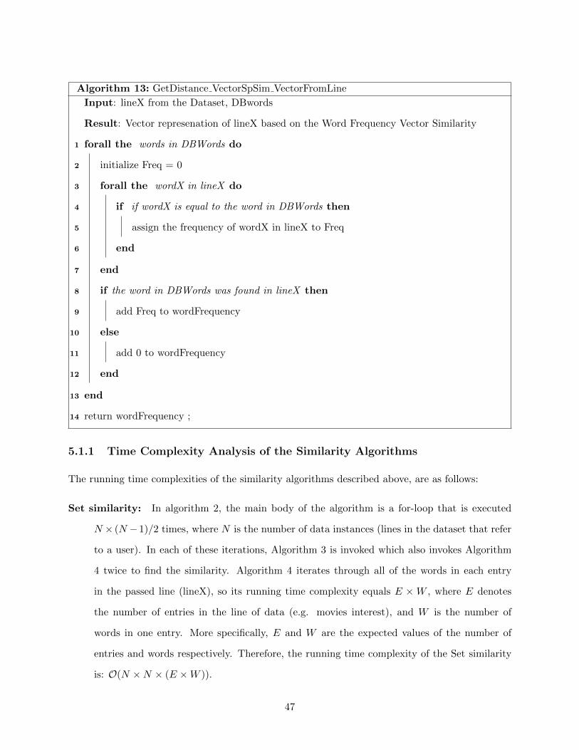
Algorithm 13: GetDistance VectorSpSim VectorFromLine
Input: lineX from the Dataset, DBwords
Result: Vector represenation of lineX based on the Word Frequency Vector Similarity
1 forall the words in DBWords do
2 initialize Freq = 0
3 forall the wordX in lineX do
4 if if wordX is equal to the word in DBWords then
5 assign the frequency of wordX in lineX to Freq
6 end
7 end
8 if the word in DBWords was found in lineX then
9 add Freq to wordFrequency
10 else
11 add 0 to wordFrequency
12 end
13 end
14 return wordFrequency ;
5.1.1 Time Complexity Analysis of the Similarity Algorithms
The running time complexities of the similarity algorithms described above, are as follows:
Set similarity: In algorithm 2, the main body of the algorithm is a for-loop that is executed
N × (N −1)/2 times, where N is the number of data instances (lines in the dataset that refer
to a user). In each of these iterations, Algorithm 3 is invoked which also invokes Algorithm
4 twice to find the similarity. Algorithm 4 iterates through all of the words in each entry
in the passed line (lineX), so its running time complexity equals E ×W , where E denotes
the number of entries in the line of data (e.g. movies interest), and W is the number of
words in one entry. More specifically, E and W are the expected values of the number of
entries and words respectively. Therefore, the running time complexity of the Set similarity
is: O(N ×N × (E ×W )).
47
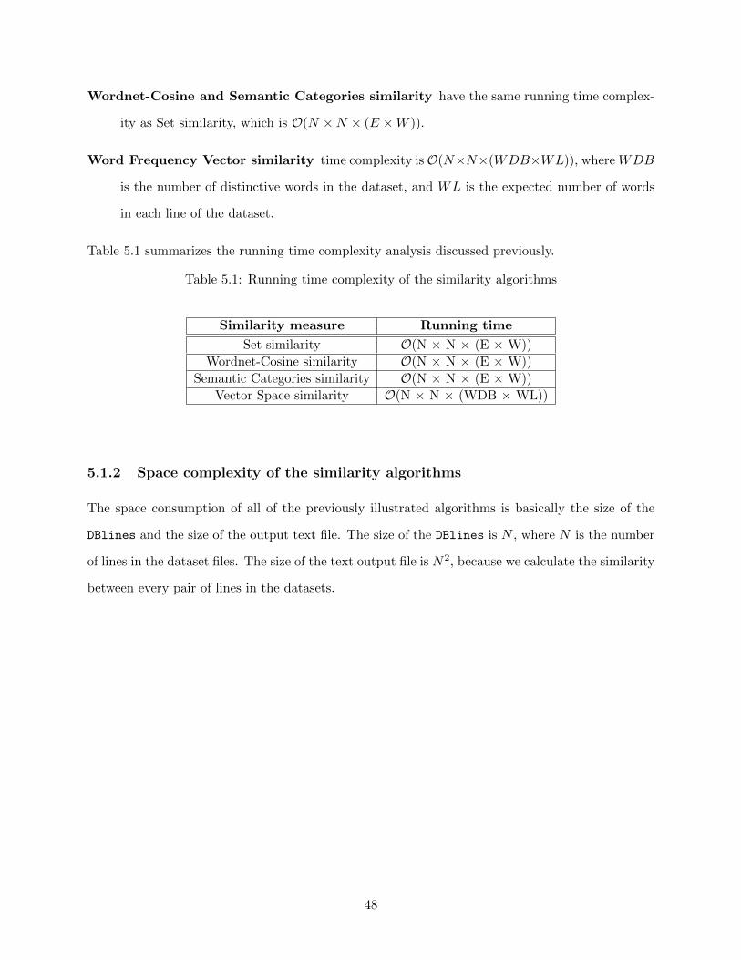
Wordnet-Cosine and Semantic Categories similarity have the same running time complex-
ity as Set similarity, which is O(N ×N × (E ×W )).
Word Frequency Vector similarity time complexity isO(N×N×(WDB×WL)), whereWDB
is the number of distinctive words in the dataset, and WL is the expected number of words
in each line of the dataset.
Table 5.1 summarizes the running time complexity analysis discussed previously.
Table 5.1: Running time complexity of the similarity algorithms
Similarity measure Running time
Set similarity O(N × N × (E × W))
Wordnet-Cosine similarity O(N × N × (E × W))
Semantic Categories similarity O(N × N × (E × W))
Vector Space similarity O(N × N × (WDB × WL))
5.1.2 Space complexity of the similarity algorithms
The space consumption of all of the previously illustrated algorithms is basically the size of the
DBlines and the size of the output text file. The size of the DBlines is N , where N is the number
of lines in the dataset files. The size of the text output file is N2, because we calculate the similarity
between every pair of lines in the datasets.
48
Chapter 6
Experiments and Results
6.1 Experiments
Several experiments have been conducted in order to evaluate the quality of different similarity
measures. In the first set of experiments, clustering was used to group the data (e.g. nodes in
profiles in Facebook) into k clusters, with k = 2, 3, 4, 5, and 6 based on the similarity measures.
The quality of the clusters was studied to find out which similarity measure produces the best
clustering results.
In the second set of experiments, the Wordnet-Cosine similarity measure was used to predict
links in a social random graph. The predictor accuracy was compared with the accuracy of a
random link predictor.
Facebook, Movielens, and DBLP data were used for the first set of experiments. The information
in the MovieLens dataset is shown in Table 6.1 (this information was taken from the read me file
of the MovieLens dataset 1). Only the id and the movie title from the MovieLens were used in
finding the similarity between all pairs of data. The id was used to reference the data tuple (row).
Tables 6.2, 6.3, and 6.4 show the first 10 records of each of these data sets respectively. In the
Facebook dataset, each row represents a Facebook user identified by an id (auto generated) and
his/her movies interest. Table 6.5 displays the size of the distance matrices used in the clustering
experiments. These matrices were first compiled by applying the four similarity measures, Cat
(Semantic Categories), (Set), Vector (Word Frequency Vector), and Wordnet (Wordnet-Cosine),
1http://grouplens.org/datasets/movielens/
49
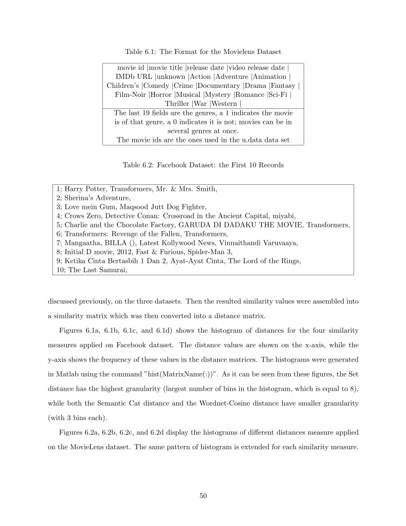
Table 6.1: The Format for the Movielens Dataset
movie id |movie title |release date |video release date |IMDb URL |unknown |Action |Adventure |Animation |
Children’s |Comedy |Crime |Documentary |Drama |Fantasy |Film-Noir |Horror |Musical |Mystery |Romance |Sci-Fi |
Thriller |War |Western |The last 19 fields are the genres, a 1 indicates the movieis of that genre, a 0 indicates it is not; movies can be in
several genres at once.The movie ids are the ones used in the u.data data set
Table 6.2: Facebook Dataset: the First 10 Records
1; Harry Potter, Transformers, Mr. & Mrs. Smith,2; Sherina’s Adventure,3; Love mein Gum, Maqsood Jutt Dog Fighter,4; Crows Zero, Detective Conan: Crossroad in the Ancient Capital, miyabi,5; Charlie and the Chocolate Factory, GARUDA DI DADAKU THE MOVIE, Transformers,6; Transformers: Revenge of the Fallen, Transformers,7; Mangaatha, BILLA (), Latest Kollywood News, Vinnaithandi Varuvaaya,8; Initial D movie, 2012, Fast & Furious, Spider-Man 3,9; Ketika Cinta Bertasbih 1 Dan 2, Ayat-Ayat Cinta, The Lord of the Rings,10; The Last Samurai,
discussed previously, on the three datasets. Then the resulted similarity values were assembled into
a similarity matrix which was then converted into a distance matrix.
Figures 6.1a, 6.1b, 6.1c, and 6.1d) shows the histogram of distances for the four similarity
measures applied on Facebook dataset. The distance values are shown on the x-axis, while the
y-axis shows the frequency of these values in the distance matrices. The histograms were generated
in Matlab using the command ”hist(MatrixName(:))”. As it can be seen from these figures, the Set
distance has the highest granularity (largest number of bins in the histogram, which is equal to 8),
while both the Semantic Cat distance and the Wordnet-Cosine distance have smaller granularity
(with 3 bins each).
Figures 6.2a, 6.2b, 6.2c, and 6.2d display the histograms of different distances measure applied
on the MovieLens dataset. The same pattern of histogram is extended for each similarity measure.
50
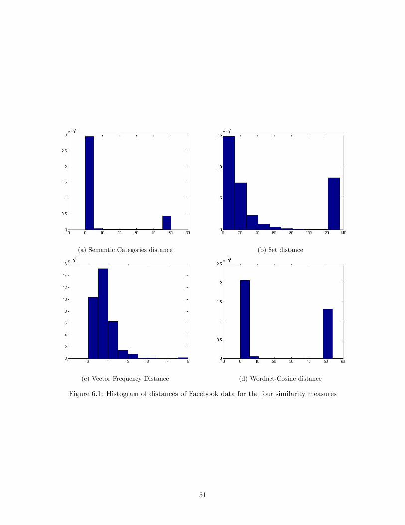
(a) Semantic Categories distance (b) Set distance
(c) Vector Frequency Distance (d) Wordnet-Cosine distance
Figure 6.1: Histogram of distances of Facebook data for the four similarity measures
51
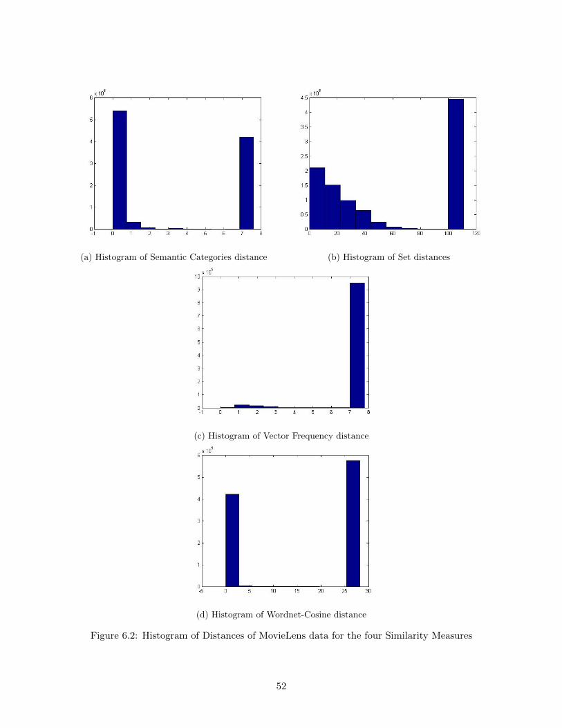
(a) Histogram of Semantic Categories distance (b) Histogram of Set distances
(c) Histogram of Vector Frequency distance
(d) Histogram of Wordnet-Cosine distance
Figure 6.2: Histogram of Distances of MovieLens data for the four Similarity Measures
52
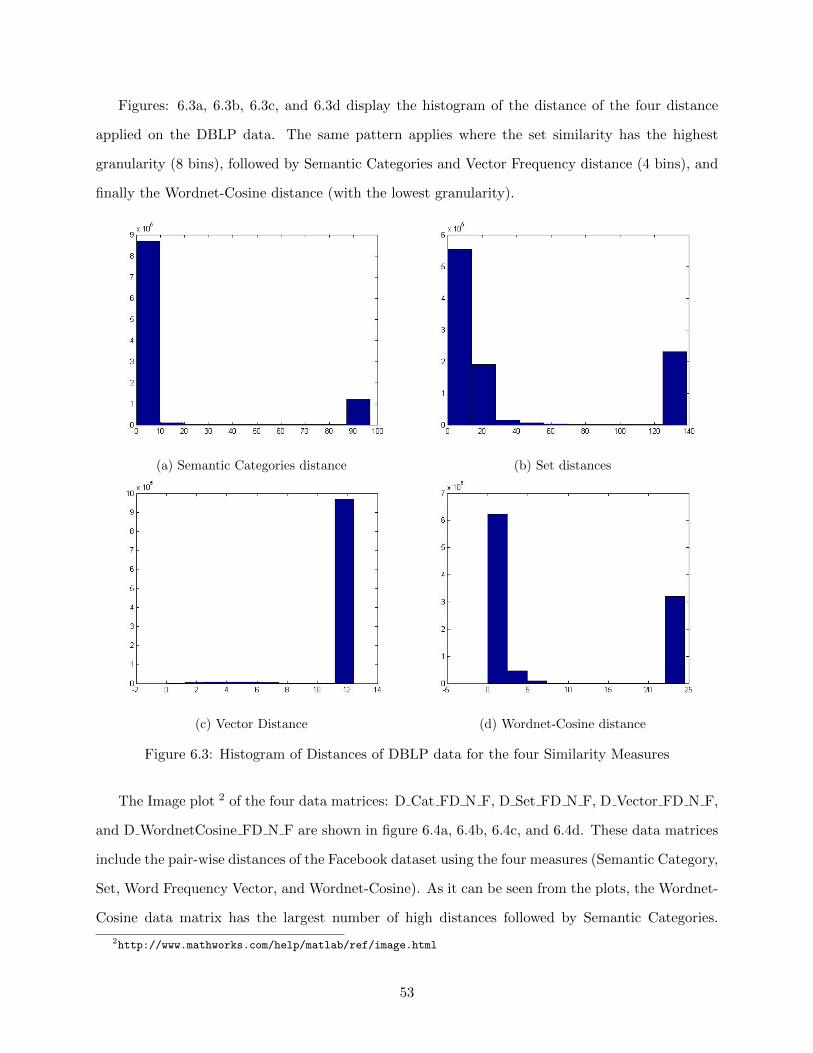
Figures: 6.3a, 6.3b, 6.3c, and 6.3d display the histogram of the distance of the four distance
applied on the DBLP data. The same pattern applies where the set similarity has the highest
granularity (8 bins), followed by Semantic Categories and Vector Frequency distance (4 bins), and
finally the Wordnet-Cosine distance (with the lowest granularity).
(a) Semantic Categories distance (b) Set distances
(c) Vector Distance (d) Wordnet-Cosine distance
Figure 6.3: Histogram of Distances of DBLP data for the four Similarity Measures
The Image plot 2 of the four data matrices: D Cat FD N F, D Set FD N F, D Vector FD N F,
and D WordnetCosine FD N F are shown in figure 6.4a, 6.4b, 6.4c, and 6.4d. These data matrices
include the pair-wise distances of the Facebook dataset using the four measures (Semantic Category,
Set, Word Frequency Vector, and Wordnet-Cosine). As it can be seen from the plots, the Wordnet-
Cosine data matrix has the largest number of high distances followed by Semantic Categories.
2http://www.mathworks.com/help/matlab/ref/image.html
53
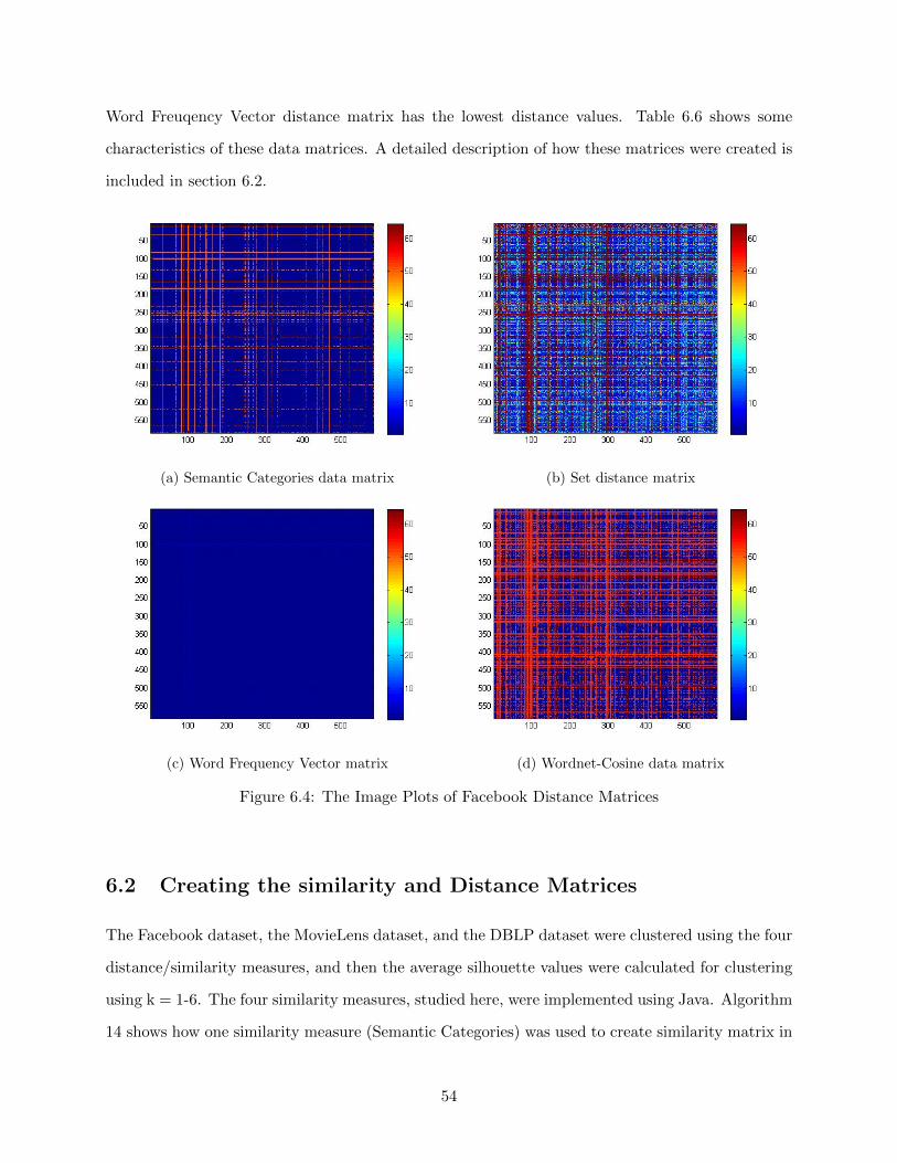
Word Freuqency Vector distance matrix has the lowest distance values. Table 6.6 shows some
characteristics of these data matrices. A detailed description of how these matrices were created is
included in section 6.2.
(a) Semantic Categories data matrix (b) Set distance matrix
(c) Word Frequency Vector matrix (d) Wordnet-Cosine data matrix
Figure 6.4: The Image Plots of Facebook Distance Matrices
6.2 Creating the similarity and Distance Matrices
The Facebook dataset, the MovieLens dataset, and the DBLP dataset were clustered using the four
distance/similarity measures, and then the average silhouette values were calculated for clustering
using k = 1-6. The four similarity measures, studied here, were implemented using Java. Algorithm
14 shows how one similarity measure (Semantic Categories) was used to create similarity matrix in
54
Matlab from the Facebook dataset. This process can be described as follows:
• An output text file is created that stores the similarity between every pair of users and that
resembles a line in the output text file. Algorithm 14 reads the similarity values for all pairs
of data (all lines in the text file) and converts them into a similarity matrix so that they can
be clustered and explored in depth.
• Algorithm 15 displays the code for converting the similarity matrix into distance matrix
(replacing the NaN values), clustering, and finding the average silhouette using Matlab. The
similarity matrix (the ”SM” prefix in the matrix name) was converted to distance matrix (the
D prefix in the matrix name) by using the equation:
d(x, y) = 1/s(x, y)− 1
[36] [14], see algorithm 15 line 1. That means:
– when s(x, y) = 0→ d(x, y) =∞ (dissimilar)
– when s(x, y) = 1→ d(x, y) = 0 (similar).
• The NaN values are replaced by maximum distance, in what is known as Imputation [56], see
algorithm 15 lines 2-9
55
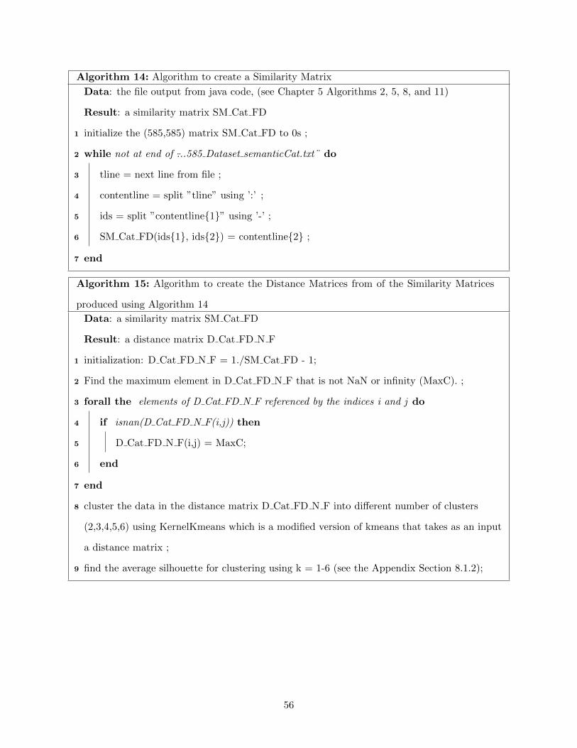
Algorithm 14: Algorithm to create a Similarity Matrix
Data: the file output from java code, (see Chapter 5 Algorithms 2, 5, 8, and 11)
Result: a similarity matrix SM Cat FD
1 initialize the (585,585) matrix SM Cat FD to 0s ;
2 while not at end of ...585 Dataset semanticCat.txt¨ do
3 tline = next line from file ;
4 contentline = split ”tline” using ’:’ ;
5 ids = split ”contentline{1}” using ’-’ ;
6 SM Cat FD(ids{1}, ids{2}) = contentline{2} ;
7 end
Algorithm 15: Algorithm to create the Distance Matrices from of the Similarity Matrices
produced using Algorithm 14
Data: a similarity matrix SM Cat FD
Result: a distance matrix D Cat FD N F
1 initialization: D Cat FD N F = 1./SM Cat FD - 1;
2 Find the maximum element in D Cat FD N F that is not NaN or infinity (MaxC). ;
3 forall the elements of D Cat FD N F referenced by the indices i and j do
4 if isnan(D Cat FD N F(i,j)) then
5 D Cat FD N F(i,j) = MaxC;
6 end
7 end
8 cluster the data in the distance matrix D Cat FD N F into different number of clusters
(2,3,4,5,6) using KernelKmeans which is a modified version of kmeans that takes as an input
a distance matrix ;
9 find the average silhouette for clustering using k = 1-6 (see the Appendix Section 8.1.2);
56
6.3 Clustering using Similarity and the Silhouette Index for Clus-
tering Validation
The results obtained by finding the similarity between the movies in the Facebook dataset, Facebook
Dataset.txt, were used to find the distance matrix which was then used to cluster the data. This
was also repeated for the Movielen and DBLP datasets.
6.3.1 Kmeans Clustering
Kmeans is a method for clustering data, and it is supported by Matlab (kmeans function) [24].
Clustering refers to the problem of grouping the data points into sets which are as tight/compact
and as separated as possible. Clustering is used as a ground truth to evaluate the similarity/distance
measures since we assume that similar profiles will be in the same cluster when one attempts to
cluster them using the similarity/distance measures. Therefore, after clustering the data using the
various distance measures, we study the quality of clusters using the Silhouette index to find out
which similarity/distance measure cluster the data the best. In this study, a modified version of
Kmeans has been used (see the Appendix Section 8.1.3)
6.3.2 Silhouette
The silhouette index has been used to measure the quality of clusters for each of the four similarity
measures. The Silhouette index captures the compactness and separation of clusters and is defined
as follows (Equation 6.2 and 6.1) [51]:
S(i) =
1− a(i)
b(i) if a(i) < b(i)
0 if a(i) = b(i)
b(i)a(i) − 1 if a(i) > b(i)
(6.1)
S(i) =b(i)− a(i)
max{a(i), b(i)}(6.2)
Where −1 ≤ S(i) ≤ 1, and i denotes data point and the quantities b(i) and a(i) are defined as
follows:
57
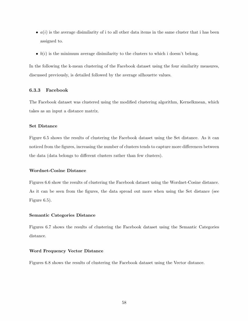
• a(i) is the average disimilarity of i to all other data items in the same cluster that i has been
assigned to.
• b(i) is the minimum average disimilarity to the clusters to which i doesn’t belong.
In the following the k-mean clustering of the Facebook dataset using the four similarity measures,
discussed previously, is detailed followed by the average silhouette values.
6.3.3 Facebook
The Facebook dataset was clustered using the modified clustering algorithm, Kernelkmean, which
takes as an input a distance matrix.
Set Distance
Figure 6.5 shows the results of clustering the Facebook dataset using the Set distance. As it can
noticed from the figures, increasing the number of clusters tends to capture more differences between
the data (data belongs to different clusters rather than few clusters).
Wordnet-Cosine Distance
Figures 6.6 show the results of clustering the Facebook dataset using the Wordnet-Cosine distance.
As it can be seen from the figures, the data spread out more when using the Set distance (see
Figure 6.5).
Semantic Categories Distance
Figures 6.7 shows the results of clustering the Facebook dataset using the Semantic Categories
distance.
Word Frequency Vector Distance
Figures 6.8 shows the results of clustering the Facebook dataset using the Vector distance.
58
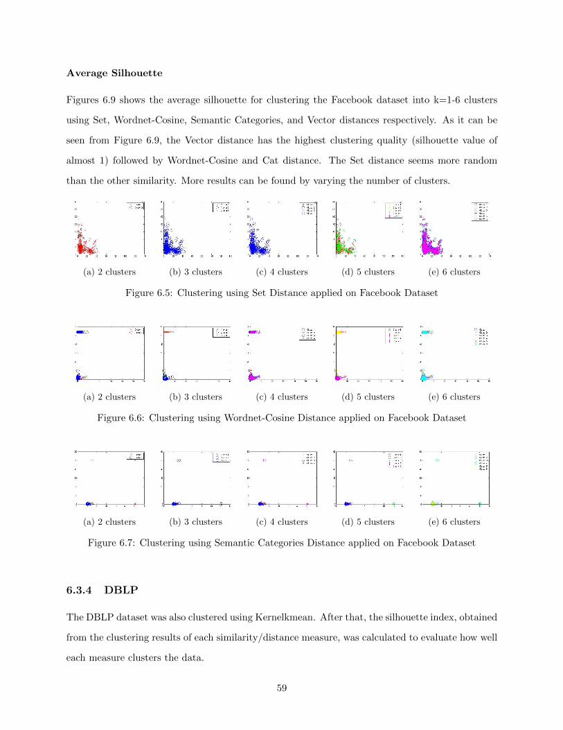
Average Silhouette
Figures 6.9 shows the average silhouette for clustering the Facebook dataset into k=1-6 clusters
using Set, Wordnet-Cosine, Semantic Categories, and Vector distances respectively. As it can be
seen from Figure 6.9, the Vector distance has the highest clustering quality (silhouette value of
almost 1) followed by Wordnet-Cosine and Cat distance. The Set distance seems more random
than the other similarity. More results can be found by varying the number of clusters.
(a) 2 clusters (b) 3 clusters (c) 4 clusters (d) 5 clusters (e) 6 clusters
Figure 6.5: Clustering using Set Distance applied on Facebook Dataset
(a) 2 clusters (b) 3 clusters (c) 4 clusters (d) 5 clusters (e) 6 clusters
Figure 6.6: Clustering using Wordnet-Cosine Distance applied on Facebook Dataset
(a) 2 clusters (b) 3 clusters (c) 4 clusters (d) 5 clusters (e) 6 clusters
Figure 6.7: Clustering using Semantic Categories Distance applied on Facebook Dataset
6.3.4 DBLP
The DBLP dataset was also clustered using Kernelkmean. After that, the silhouette index, obtained
from the clustering results of each similarity/distance measure, was calculated to evaluate how well
each measure clusters the data.
59
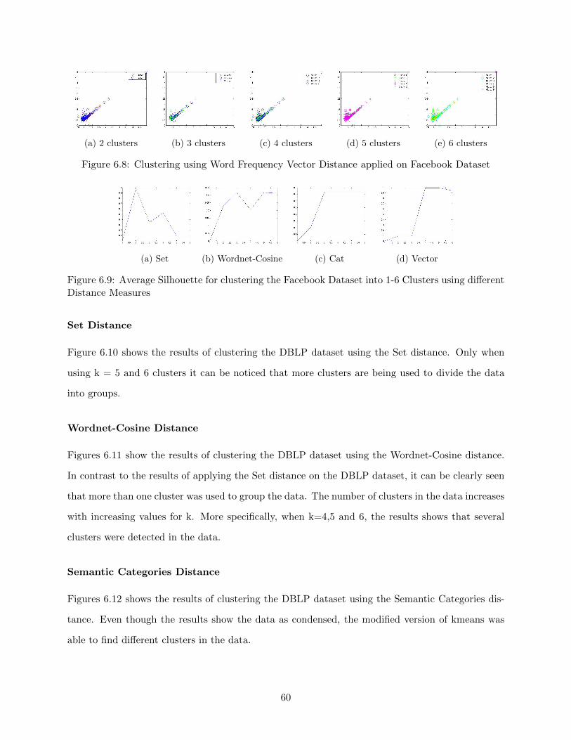
(a) 2 clusters (b) 3 clusters (c) 4 clusters (d) 5 clusters (e) 6 clusters
Figure 6.8: Clustering using Word Frequency Vector Distance applied on Facebook Dataset
(a) Set (b) Wordnet-Cosine (c) Cat (d) Vector
Figure 6.9: Average Silhouette for clustering the Facebook Dataset into 1-6 Clusters using differentDistance Measures
Set Distance
Figure 6.10 shows the results of clustering the DBLP dataset using the Set distance. Only when
using k = 5 and 6 clusters it can be noticed that more clusters are being used to divide the data
into groups.
Wordnet-Cosine Distance
Figures 6.11 show the results of clustering the DBLP dataset using the Wordnet-Cosine distance.
In contrast to the results of applying the Set distance on the DBLP dataset, it can be clearly seen
that more than one cluster was used to group the data. The number of clusters in the data increases
with increasing values for k. More specifically, when k=4,5 and 6, the results shows that several
clusters were detected in the data.
Semantic Categories Distance
Figures 6.12 shows the results of clustering the DBLP dataset using the Semantic Categories dis-
tance. Even though the results show the data as condensed, the modified version of kmeans was
able to find different clusters in the data.
60
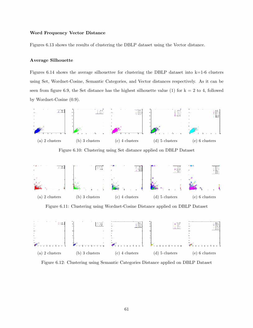
Word Frequency Vector Distance
Figures 6.13 shows the results of clustering the DBLP dataset using the Vector distance.
Average Silhouette
Figures 6.14 shows the average silhouettee for clustering the DBLP dataset into k=1-6 clusters
using Set, Wordnet-Cosine, Semantic Categories, and Vector distances respectively. As it can be
seen from figure 6.9, the Set distance has the highest silhouette value (1) for k = 2 to 4, followed
by Wordnet-Cosine (0.9).
(a) 2 clusters (b) 3 clusters (c) 4 clusters (d) 5 clusters (e) 6 clusters
Figure 6.10: Clustering using Set distance applied on DBLP Dataset
(a) 2 clusters (b) 3 clusters (c) 4 clusters (d) 5 clusters (e) 6 clusters
Figure 6.11: Clustering using Wordnet-Cosine Distance applied on DBLP Dataset
(a) 2 clusters (b) 3 clusters (c) 4 clusters (d) 5 clusters (e) 6 clusters
Figure 6.12: Clustering using Semantic Categories Distance applied on DBLP Dataset
61
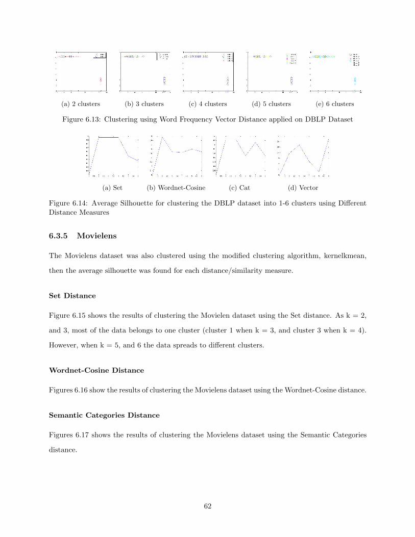
(a) 2 clusters (b) 3 clusters (c) 4 clusters (d) 5 clusters (e) 6 clusters
Figure 6.13: Clustering using Word Frequency Vector Distance applied on DBLP Dataset
(a) Set (b) Wordnet-Cosine (c) Cat (d) Vector
Figure 6.14: Average Silhouette for clustering the DBLP dataset into 1-6 clusters using DifferentDistance Measures
6.3.5 Movielens
The Movielens dataset was also clustered using the modified clustering algorithm, kernelkmean,
then the average silhouette was found for each distance/similarity measure.
Set Distance
Figure 6.15 shows the results of clustering the Movielen dataset using the Set distance. As k = 2,
and 3, most of the data belongs to one cluster (cluster 1 when k = 3, and cluster 3 when k = 4).
However, when k = 5, and 6 the data spreads to different clusters.
Wordnet-Cosine Distance
Figures 6.16 show the results of clustering the Movielens dataset using the Wordnet-Cosine distance.
Semantic Categories Distance
Figures 6.17 shows the results of clustering the Movielens dataset using the Semantic Categories
distance.
62
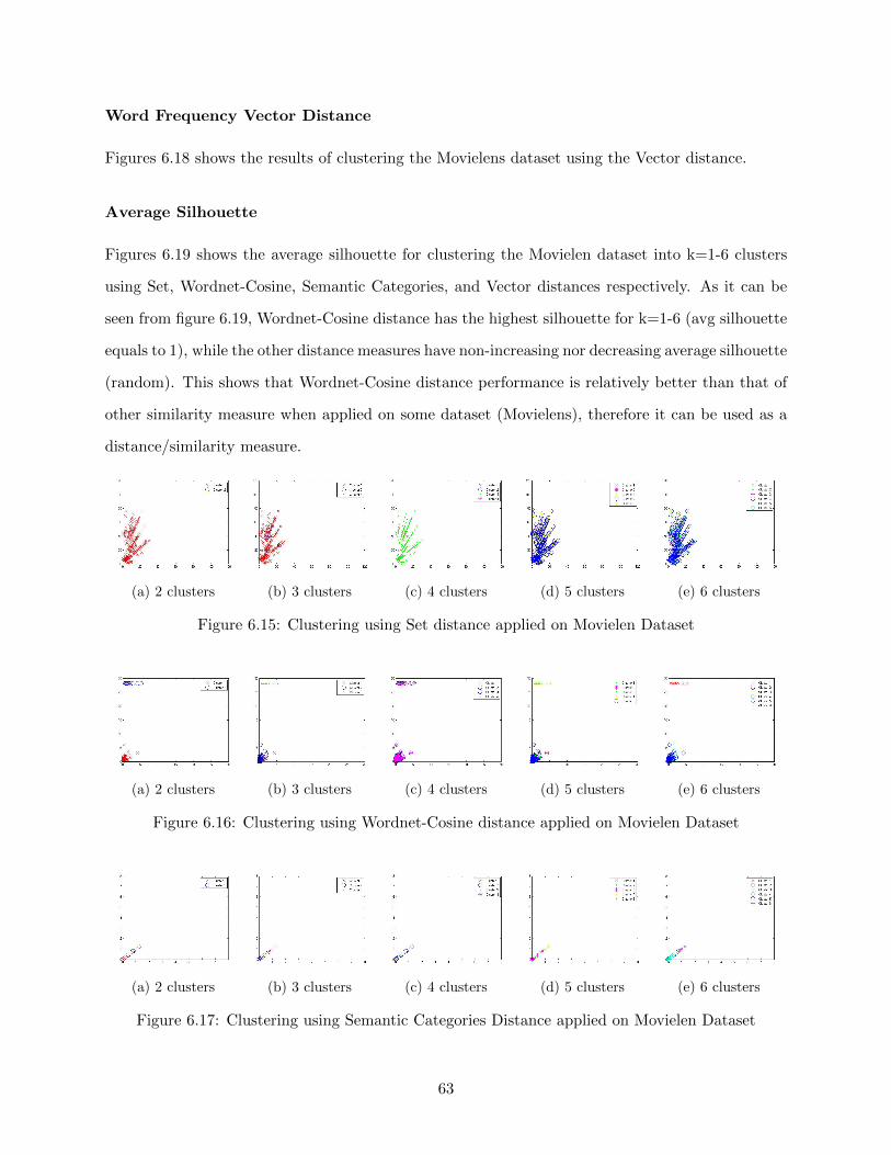
Word Frequency Vector Distance
Figures 6.18 shows the results of clustering the Movielens dataset using the Vector distance.
Average Silhouette
Figures 6.19 shows the average silhouette for clustering the Movielen dataset into k=1-6 clusters
using Set, Wordnet-Cosine, Semantic Categories, and Vector distances respectively. As it can be
seen from figure 6.19, Wordnet-Cosine distance has the highest silhouette for k=1-6 (avg silhouette
equals to 1), while the other distance measures have non-increasing nor decreasing average silhouette
(random). This shows that Wordnet-Cosine distance performance is relatively better than that of
other similarity measure when applied on some dataset (Movielens), therefore it can be used as a
distance/similarity measure.
(a) 2 clusters (b) 3 clusters (c) 4 clusters (d) 5 clusters (e) 6 clusters
Figure 6.15: Clustering using Set distance applied on Movielen Dataset
(a) 2 clusters (b) 3 clusters (c) 4 clusters (d) 5 clusters (e) 6 clusters
Figure 6.16: Clustering using Wordnet-Cosine distance applied on Movielen Dataset
(a) 2 clusters (b) 3 clusters (c) 4 clusters (d) 5 clusters (e) 6 clusters
Figure 6.17: Clustering using Semantic Categories Distance applied on Movielen Dataset
63
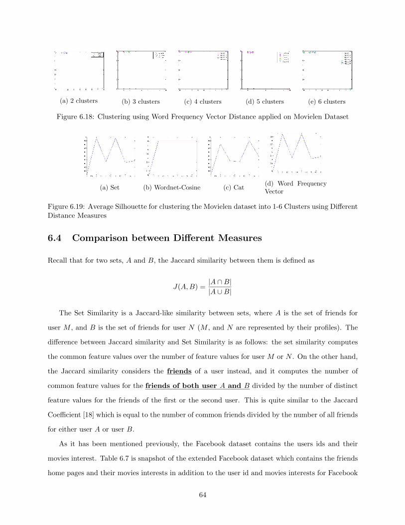
(a) 2 clusters (b) 3 clusters (c) 4 clusters (d) 5 clusters (e) 6 clusters
Figure 6.18: Clustering using Word Frequency Vector Distance applied on Movielen Dataset
(a) Set (b) Wordnet-Cosine (c) Cat(d) Word FrequencyVector
Figure 6.19: Average Silhouette for clustering the Movielen dataset into 1-6 Clusters using DifferentDistance Measures
6.4 Comparison between Different Measures
Recall that for two sets, A and B, the Jaccard similarity between them is defined as
J(A,B) =|A ∩B||A ∪B|
The Set Similarity is a Jaccard-like similarity between sets, where A is the set of friends for
user M , and B is the set of friends for user N (M , and N are represented by their profiles). The
difference between Jaccard similarity and Set Similarity is as follows: the set similarity computes
the common feature values over the number of feature values for user M or N . On the other hand,
the Jaccard similarity considers the friends of a user instead, and it computes the number of
common feature values for the friends of both user A and B divided by the number of distinct
feature values for the friends of the first or the second user. This is quite similar to the Jaccard
Coefficient [18] which is equal to the number of common friends divided by the number of all friends
for either user A or user B.
As it has been mentioned previously, the Facebook dataset contains the users ids and their
movies interest. Table 6.7 is snapshot of the extended Facebook dataset which contains the friends
home pages and their movies interests in addition to the user id and movies interests for Facebook
64
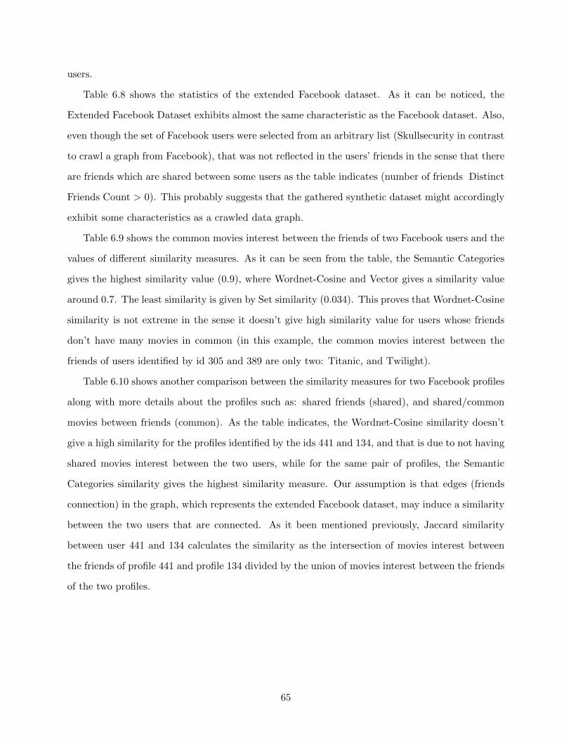
users.
Table 6.8 shows the statistics of the extended Facebook dataset. As it can be noticed, the
Extended Facebook Dataset exhibits almost the same characteristic as the Facebook dataset. Also,
even though the set of Facebook users were selected from an arbitrary list (Skullsecurity in contrast
to crawl a graph from Facebook), that was not reflected in the users’ friends in the sense that there
are friends which are shared between some users as the table indicates (number of friends Distinct
Friends Count > 0). This probably suggests that the gathered synthetic dataset might accordingly
exhibit some characteristics as a crawled data graph.
Table 6.9 shows the common movies interest between the friends of two Facebook users and the
values of different similarity measures. As it can be seen from the table, the Semantic Categories
gives the highest similarity value (0.9), where Wordnet-Cosine and Vector gives a similarity value
around 0.7. The least similarity is given by Set similarity (0.034). This proves that Wordnet-Cosine
similarity is not extreme in the sense it doesn’t give high similarity value for users whose friends
don’t have many movies in common (in this example, the common movies interest between the
friends of users identified by id 305 and 389 are only two: Titanic, and Twilight).
Table 6.10 shows another comparison between the similarity measures for two Facebook profiles
along with more details about the profiles such as: shared friends (shared), and shared/common
movies between friends (common). As the table indicates, the Wordnet-Cosine similarity doesn’t
give a high similarity for the profiles identified by the ids 441 and 134, and that is due to not having
shared movies interest between the two users, while for the same pair of profiles, the Semantic
Categories similarity gives the highest similarity measure. Our assumption is that edges (friends
connection) in the graph, which represents the extended Facebook dataset, may induce a similarity
between the two users that are connected. As it been mentioned previously, Jaccard similarity
between user 441 and 134 calculates the similarity as the intersection of movies interest between
the friends of profile 441 and profile 134 divided by the union of movies interest between the friends
of the two profiles.
65
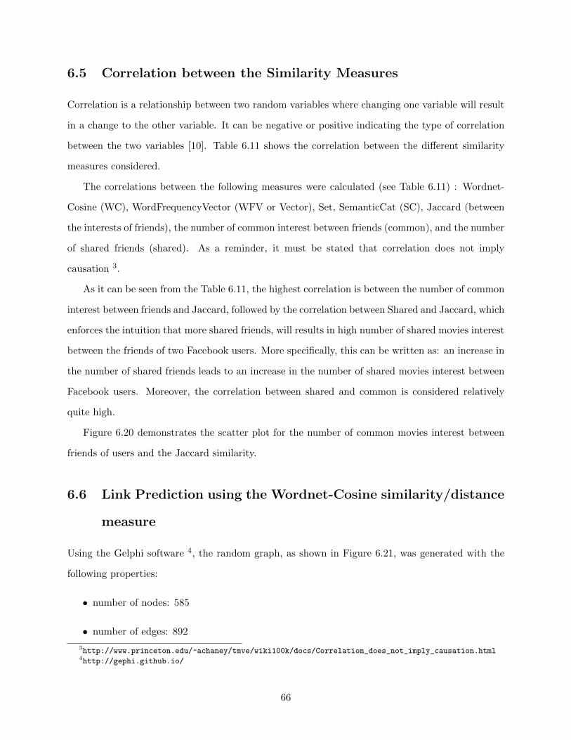
6.5 Correlation between the Similarity Measures
Correlation is a relationship between two random variables where changing one variable will result
in a change to the other variable. It can be negative or positive indicating the type of correlation
between the two variables [10]. Table 6.11 shows the correlation between the different similarity
measures considered.
The correlations between the following measures were calculated (see Table 6.11) : Wordnet-
Cosine (WC), WordFrequencyVector (WFV or Vector), Set, SemanticCat (SC), Jaccard (between
the interests of friends), the number of common interest between friends (common), and the number
of shared friends (shared). As a reminder, it must be stated that correlation does not imply
causation 3.
As it can be seen from the Table 6.11, the highest correlation is between the number of common
interest between friends and Jaccard, followed by the correlation between Shared and Jaccard, which
enforces the intuition that more shared friends, will results in high number of shared movies interest
between the friends of two Facebook users. More specifically, this can be written as: an increase in
the number of shared friends leads to an increase in the number of shared movies interest between
Facebook users. Moreover, the correlation between shared and common is considered relatively
quite high.
Figure 6.20 demonstrates the scatter plot for the number of common movies interest between
friends of users and the Jaccard similarity.
6.6 Link Prediction using the Wordnet-Cosine similarity/distance
measure
Using the Gelphi software 4, the random graph, as shown in Figure 6.21, was generated with the
following properties:
• number of nodes: 585
• number of edges: 892
3http://www.princeton.edu/~achaney/tmve/wiki100k/docs/Correlation_does_not_imply_causation.html4http://gephi.github.io/
66
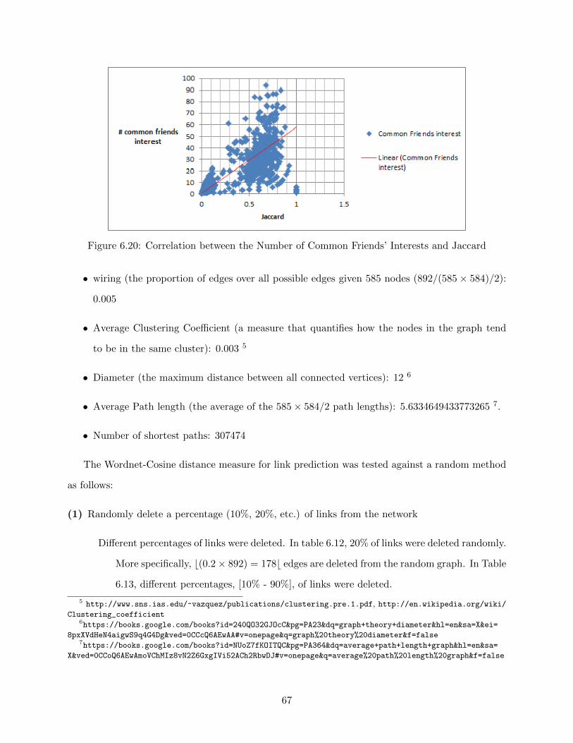
Figure 6.20: Correlation between the Number of Common Friends’ Interests and Jaccard
• wiring (the proportion of edges over all possible edges given 585 nodes (892/(585× 584)/2):
0.005
• Average Clustering Coefficient (a measure that quantifies how the nodes in the graph tend
to be in the same cluster): 0.003 5
• Diameter (the maximum distance between all connected vertices): 12 6
• Average Path length (the average of the 585× 584/2 path lengths): 5.6334649433773265 7.
• Number of shortest paths: 307474
The Wordnet-Cosine distance measure for link prediction was tested against a random method
as follows:
(1) Randomly delete a percentage (10%, 20%, etc.) of links from the network
Different percentages of links were deleted. In table 6.12, 20% of links were deleted randomly.
More specifically, b(0.2× 892) = 178b edges are deleted from the random graph. In Table
6.13, different percentages, [10% - 90%], of links were deleted.
5 http://www.sns.ias.edu/~vazquez/publications/clustering.pre.1.pdf, http://en.wikipedia.org/wiki/Clustering_coefficient
6https://books.google.com/books?id=240QO32GJOcC&pg=PA23&dq=graph+theory+diameter&hl=en&sa=X&ei=
8pxXVdHeN4aigwS9q4G4Dg&ved=0CCcQ6AEwAA#v=onepage&q=graph%20theory%20diameter&f=false7https://books.google.com/books?id=NUoZ7fKOITQC&pg=PA364&dq=average+path+length+graph&hl=en&sa=
X&ved=0CCoQ6AEwAmoVChMIz8vN2Z6GxgIVi52ACh2RbwDJ#v=onepage&q=average%20path%20length%20graph&f=false
67
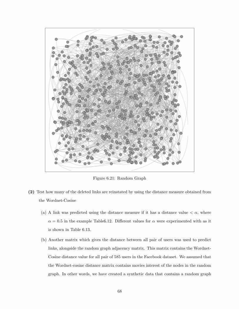
Figure 6.21: Random Graph
(2) Test how many of the deleted links are reinstated by using the distance measure obtained from
the Wordnet-Cosine
(a) A link was predicted using the distance measure if it has a distance value < α, where
α = 0.5 in the example Table6.12. Different values for α were experimented with as it
is shown in Table 6.13.
(b) Another matrix which gives the distance between all pair of users was used to predict
links, alongside the random graph adjacency matrix. This matrix contains the Wordnet-
Cosine distance value for all pair of 585 users in the Facebook dataset. We assumed that
the Wordnet-cosine distance matrix contains movies interest of the nodes in the random
graph. In other words, we have created a synthetic data that contains a random graph
68
(generated by Gelphi) and movies interest of different users (generated by Skullsecurity
list).
(3) Evaluate the number of links reinstated by a random procedure
A random binary vector, x, of {0, 1} values, was generated with a size equal to the number
of deleted edges, that is, here the random vector of dimension 178 of 1s/0s to mean that
a link is predicted/not predicted.
(4) Evaluate how different are the results from (2) and (3).
Calculate the number of predicted links using (2) and (3): The exclusive-or operator is
applied to the two adjacency matrices: for the prediction based on distance and random,
and the random graph after deleting from it the percentage of links, mentioned above.
From Table 6.12, it can be concluded that the Wordnet-cosine distance outperformed the random
link prediction method by a factor of (117 − 90) ÷ 117 × 100 = 23.07% based on the experiment
conducted. Furthermore, it can be seen that the Wordnet-Cosine distance was able to predict
(117÷ 178)× 100 = 65.73% of deleted edges (links). Based on the detailed experiment above, the
accuracy of predicting links using Random is 90÷ 178× 100 = 50.56%.
The accuracy of random link prediction and Wordnet-Cosine distance link prediction, using
different values for deleted edges and distance threshold, is shown in the Table 6.13. The table
shows the number of deleted edges from the random graph (edges del), the percentage of deleted
edges (% edges del), the Distance Threshold (Dist T), the number of predicted links using Random
(predicted Ran), the number of predicted links using Wordnet-Cosine distance (predicted Dist), the
Random predictor accuracy (Rand Acy), and the Wordnet-Cosine predictor accuracy (dist Acy).
For the Wordnet-Cosine distance link prediction, a link was predicted if the distance between
the two nodes is less than the Distance Threshold (Dist T). The accuracy of the random predictor
ranges from 37.08% to 58.43%, while the accuracy of the Wordnet-Cosine distance predictor ranges
from 0.056 to 65.73%. Which means that Wordnet-Cosine distance-based predictor achieves higher
accuracy than the random predictor (65.73% v.s. 58.43%). See the probability of correctness
for the random predictor [35]. As it can be seen from Table 6.13, the Wordnet-Cosine distance
link predictor, has a higher accuracy for most cases where the Distance Threshold (Dist T) =
69
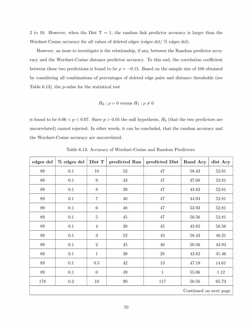
2 to 10. However, when the Dist T = 1, the random link predictor accuracy is larger than the
Wordnet-Cosine accuracy for all values of deleted edges (edges del/ % edges del).
However, an issue to investigate is the relationship, if any, between the Random predictor accu-
racy and the Wordnet-Cosine distance predictor accuracy. To this end, the correlation coefficient
between these two predictions is found to be ρ = −0.15. Based on the sample size of 108 obtained
by considering all combinations of percentages of deleted edge pairs and distance thresholds (see
Table 6.13), the p-value for the statistical test
H0 : ρ = 0 versus H1 : ρ 6= 0
is found to be 0.06 < p < 0.07. Since p > 0.05 the null hypothesis, H0 (that the two predictors are
uncorrelated) cannot rejected. In other words, it can be concluded, that the random accuracy and
the Wordnet-Cosine accuracy are uncorrelated.
Table 6.13: Accuracy of Wordnet-Cosine and Random Predictors
edges del % edges del Dist T predicted Ran predicted Dist Rand Acy dist Acy
89 0.1 10 52 47 58.43 52.81
89 0.1 9 33 47 37.08 52.81
89 0.1 8 39 47 43.82 52.81
89 0.1 7 40 47 44.94 52.81
89 0.1 6 48 47 53.93 52.81
89 0.1 5 45 47 50.56 52.81
89 0.1 4 39 45 43.82 50.56
89 0.1 3 52 43 58.43 48.31
89 0.1 2 45 40 50.56 44.94
89 0.1 1 39 28 43.82 31.46
89 0.1 0.5 42 13 47.19 14.61
89 0.1 0 49 1 55.06 1.12
178 0.2 10 90 117 50.56 65.73
Continued on next page
70
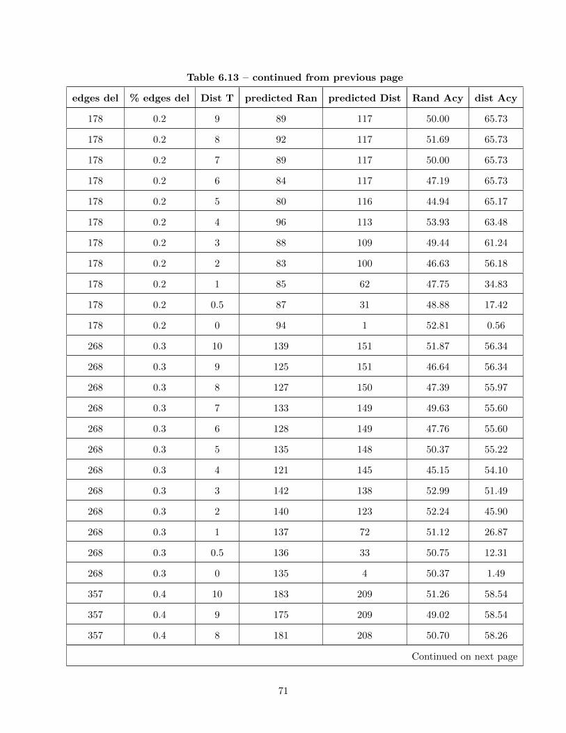
Table 6.13 – continued from previous page
edges del % edges del Dist T predicted Ran predicted Dist Rand Acy dist Acy
178 0.2 9 89 117 50.00 65.73
178 0.2 8 92 117 51.69 65.73
178 0.2 7 89 117 50.00 65.73
178 0.2 6 84 117 47.19 65.73
178 0.2 5 80 116 44.94 65.17
178 0.2 4 96 113 53.93 63.48
178 0.2 3 88 109 49.44 61.24
178 0.2 2 83 100 46.63 56.18
178 0.2 1 85 62 47.75 34.83
178 0.2 0.5 87 31 48.88 17.42
178 0.2 0 94 1 52.81 0.56
268 0.3 10 139 151 51.87 56.34
268 0.3 9 125 151 46.64 56.34
268 0.3 8 127 150 47.39 55.97
268 0.3 7 133 149 49.63 55.60
268 0.3 6 128 149 47.76 55.60
268 0.3 5 135 148 50.37 55.22
268 0.3 4 121 145 45.15 54.10
268 0.3 3 142 138 52.99 51.49
268 0.3 2 140 123 52.24 45.90
268 0.3 1 137 72 51.12 26.87
268 0.3 0.5 136 33 50.75 12.31
268 0.3 0 135 4 50.37 1.49
357 0.4 10 183 209 51.26 58.54
357 0.4 9 175 209 49.02 58.54
357 0.4 8 181 208 50.70 58.26
Continued on next page
71
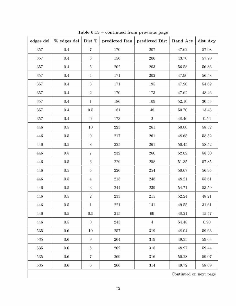
Table 6.13 – continued from previous page
edges del % edges del Dist T predicted Ran predicted Dist Rand Acy dist Acy
357 0.4 7 170 207 47.62 57.98
357 0.4 6 156 206 43.70 57.70
357 0.4 5 202 203 56.58 56.86
357 0.4 4 171 202 47.90 56.58
357 0.4 3 171 195 47.90 54.62
357 0.4 2 170 173 47.62 48.46
357 0.4 1 186 109 52.10 30.53
357 0.4 0.5 181 48 50.70 13.45
357 0.4 0 173 2 48.46 0.56
446 0.5 10 223 261 50.00 58.52
446 0.5 9 217 261 48.65 58.52
446 0.5 8 225 261 50.45 58.52
446 0.5 7 232 260 52.02 58.30
446 0.5 6 229 258 51.35 57.85
446 0.5 5 226 254 50.67 56.95
446 0.5 4 215 248 48.21 55.61
446 0.5 3 244 239 54.71 53.59
446 0.5 2 233 215 52.24 48.21
446 0.5 1 221 141 49.55 31.61
446 0.5 0.5 215 69 48.21 15.47
446 0.5 0 243 4 54.48 0.90
535 0.6 10 257 319 48.04 59.63
535 0.6 9 264 319 49.35 59.63
535 0.6 8 262 318 48.97 59.44
535 0.6 7 269 316 50.28 59.07
535 0.6 6 266 314 49.72 58.69
Continued on next page
72
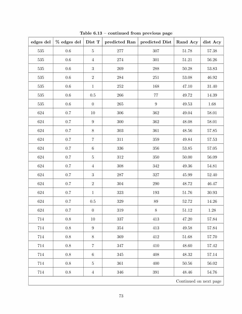
Table 6.13 – continued from previous page
edges del % edges del Dist T predicted Ran predicted Dist Rand Acy dist Acy
535 0.6 5 277 307 51.78 57.38
535 0.6 4 274 301 51.21 56.26
535 0.6 3 269 288 50.28 53.83
535 0.6 2 284 251 53.08 46.92
535 0.6 1 252 168 47.10 31.40
535 0.6 0.5 266 77 49.72 14.39
535 0.6 0 265 9 49.53 1.68
624 0.7 10 306 362 49.04 58.01
624 0.7 9 300 362 48.08 58.01
624 0.7 8 303 361 48.56 57.85
624 0.7 7 311 359 49.84 57.53
624 0.7 6 336 356 53.85 57.05
624 0.7 5 312 350 50.00 56.09
624 0.7 4 308 342 49.36 54.81
624 0.7 3 287 327 45.99 52.40
624 0.7 2 304 290 48.72 46.47
624 0.7 1 323 193 51.76 30.93
624 0.7 0.5 329 89 52.72 14.26
624 0.7 0 319 8 51.12 1.28
714 0.8 10 337 413 47.20 57.84
714 0.8 9 354 413 49.58 57.84
714 0.8 8 369 412 51.68 57.70
714 0.8 7 347 410 48.60 57.42
714 0.8 6 345 408 48.32 57.14
714 0.8 5 361 400 50.56 56.02
714 0.8 4 346 391 48.46 54.76
Continued on next page
73
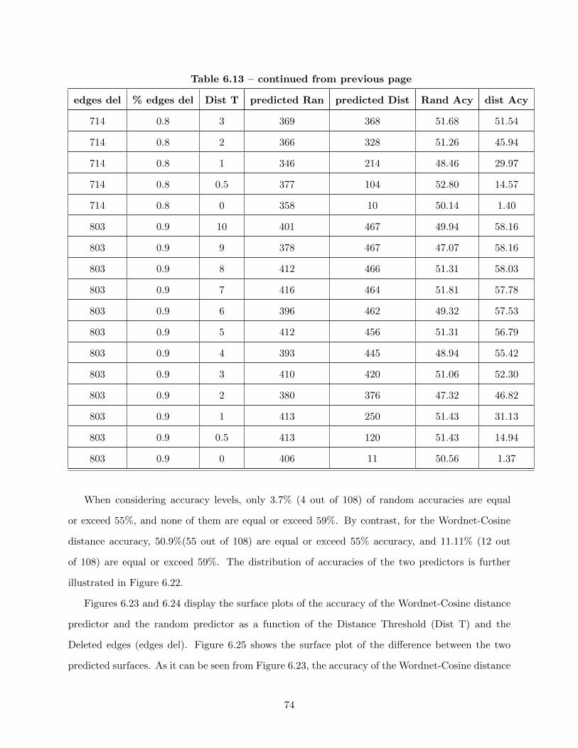
Table 6.13 – continued from previous page
edges del % edges del Dist T predicted Ran predicted Dist Rand Acy dist Acy
714 0.8 3 369 368 51.68 51.54
714 0.8 2 366 328 51.26 45.94
714 0.8 1 346 214 48.46 29.97
714 0.8 0.5 377 104 52.80 14.57
714 0.8 0 358 10 50.14 1.40
803 0.9 10 401 467 49.94 58.16
803 0.9 9 378 467 47.07 58.16
803 0.9 8 412 466 51.31 58.03
803 0.9 7 416 464 51.81 57.78
803 0.9 6 396 462 49.32 57.53
803 0.9 5 412 456 51.31 56.79
803 0.9 4 393 445 48.94 55.42
803 0.9 3 410 420 51.06 52.30
803 0.9 2 380 376 47.32 46.82
803 0.9 1 413 250 51.43 31.13
803 0.9 0.5 413 120 51.43 14.94
803 0.9 0 406 11 50.56 1.37
When considering accuracy levels, only 3.7% (4 out of 108) of random accuracies are equal
or exceed 55%, and none of them are equal or exceed 59%. By contrast, for the Wordnet-Cosine
distance accuracy, 50.9%(55 out of 108) are equal or exceed 55% accuracy, and 11.11% (12 out
of 108) are equal or exceed 59%. The distribution of accuracies of the two predictors is further
illustrated in Figure 6.22.
Figures 6.23 and 6.24 display the surface plots of the accuracy of the Wordnet-Cosine distance
predictor and the random predictor as a function of the Distance Threshold (Dist T) and the
Deleted edges (edges del). Figure 6.25 shows the surface plot of the difference between the two
predicted surfaces. As it can be seen from Figure 6.23, the accuracy of the Wordnet-Cosine distance
74
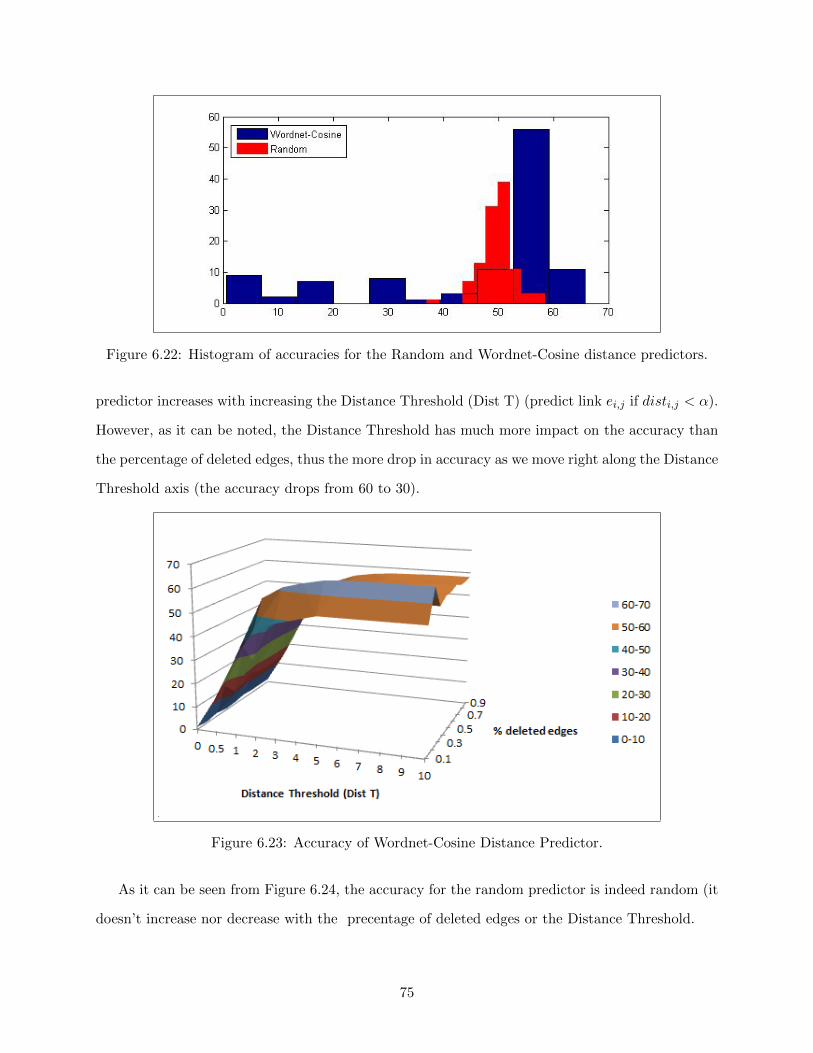
Figure 6.22: Histogram of accuracies for the Random and Wordnet-Cosine distance predictors.
predictor increases with increasing the Distance Threshold (Dist T) (predict link ei,j if disti,j < α).
However, as it can be noted, the Distance Threshold has much more impact on the accuracy than
the percentage of deleted edges, thus the more drop in accuracy as we move right along the Distance
Threshold axis (the accuracy drops from 60 to 30).
Figure 6.23: Accuracy of Wordnet-Cosine Distance Predictor.
As it can be seen from Figure 6.24, the accuracy for the random predictor is indeed random (it
doesn’t increase nor decrease with the precentage of deleted edges or the Distance Threshold.
75
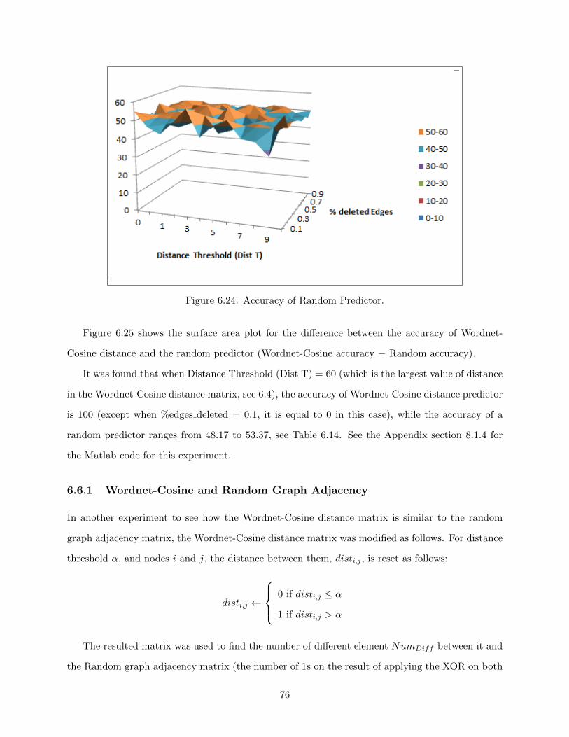
Figure 6.24: Accuracy of Random Predictor.
Figure 6.25 shows the surface area plot for the difference between the accuracy of Wordnet-
Cosine distance and the random predictor (Wordnet-Cosine accuracy − Random accuracy).
It was found that when Distance Threshold (Dist T) = 60 (which is the largest value of distance
in the Wordnet-Cosine distance matrix, see 6.4), the accuracy of Wordnet-Cosine distance predictor
is 100 (except when %edges deleted = 0.1, it is equal to 0 in this case), while the accuracy of a
random predictor ranges from 48.17 to 53.37, see Table 6.14. See the Appendix section 8.1.4 for
the Matlab code for this experiment.
6.6.1 Wordnet-Cosine and Random Graph Adjacency
In another experiment to see how the Wordnet-Cosine distance matrix is similar to the random
graph adjacency matrix, the Wordnet-Cosine distance matrix was modified as follows. For distance
threshold α, and nodes i and j, the distance between them, disti,j , is reset as follows:
disti,j ←
0 if disti,j ≤ α
1 if disti,j > α
The resulted matrix was used to find the number of different element NumDiff between it and
the Random graph adjacency matrix (the number of 1s on the result of applying the XOR on both
76
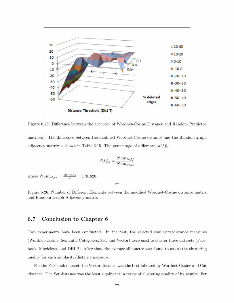
Figure 6.25: Difference between the accuracy of Wordnet-Cosine Distance and Random Predictor
matrices). The difference between the modified Wordnet-Cosine distance and the Random graph
adjacency matrix is shown in Table 6.15. The percentage of difference, diff%
diff% =NumDiff
Numedges
where Numedges = 585×5842 = 170, 820.
Figure 6.26: Number of Different Elements between the modified Wordnet-Cosine distance matrixand Random Graph Adjacency matrix
6.7 Conclusion to Chapter 6
Two experiments have been conducted. In the first, the selected similarity/distance measures
(Wordnet-Cosine, Semantic Categories, Set, and Vector) were used to cluster three datasets (Face-
book, Movielens, and DBLP). After that, the average silhouette was found to assess the clustering
quality for each similarity/distance measure.
For the Facebook dataset, the Vector distance was the best followed by Wordnet-Cosine and Cat
distance. The Set distance was the least significant in terms of clustering quality of its results. For
77
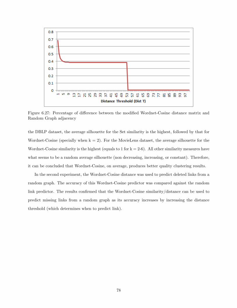
Figure 6.27: Percentage of difference between the modified Wordnet-Cosine distance matrix andRandom Graph adjacency
the DBLP dataset, the average silhouette for the Set similarity is the highest, followed by that for
Wordnet-Cosine (specially when k = 2). For the MovieLens dataset, the average silhouette for the
Wordnet-Cosine similarity is the highest (equals to 1 for k = 2-6). All other similarity measures have
what seems to be a random average silhouette (non decreasing, increasing, or constant). Therefore,
it can be concluded that Wordnet-Cosine, on average, produces better quality clustering results.
In the second experiment, the Wordnet-Cosine distance was used to predict deleted links from a
random graph. The accuracy of this Wordnet-Cosine predictor was compared against the random
link predictor. The results confirmed that the Wordnet-Cosine similarity/distance can be used to
predict missing links from a random graph as its accuracy increases by increasing the distance
threshold (which determines when to predict link).
78
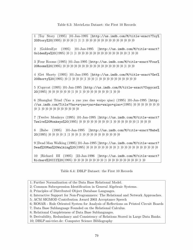
Table 6.3: MovieLens Dataset: the First 10 Records
1 |Toy Story (1995) |01-Jan-1995 ||http://us.imdb.com/M/title-exact?Toy%20Story%20(1995) |0 |0 |0 |1 |1 |1 |0 |0 |0 |0 |0 |0 |0 |0 |0 |0 |0 |0 |0
2 |GoldenEye (1995) |01-Jan-1995 ||http://us.imdb.com/M/title-exact?GoldenEye%20(1995) |0 |1 |1 |0 |0 |0 |0 |0 |0 |0 |0 |0 |0 |0 |0 |0 |1 |0 |0
3 |Four Rooms (1995) |01-Jan-1995 ||http://us.imdb.com/M/title-exact?Four%20Rooms%20(1995) |0 |0 |0 |0 |0 |0 |0 |0 |0 |0 |0 |0 |0 |0 |0 |0 |1 |0 |0
4 |Get Shorty (1995) |01-Jan-1995 ||http://us.imdb.com/M/title-exact?Get%20Shorty%20(1995) |0 |1 |0 |0 |0 |1 |0 |0 |1 |0 |0 |0 |0 |0 |0 |0 |0 |0 |0
5 |Copycat (1995) |01-Jan-1995 ||http://us.imdb.com/M/title-exact?Copycat%20(1995) |0 |0 |0 |0 |0 |0 |1 |0 |1 |0 |0 |0 |0 |0 |0 |0 |1 |0 |0
6 |Shanghai Triad (Yao a yao yao dao waipo qiao) (1995) |01-Jan-1995 ||http://us.imdb.com/Title?Yao+a+yao+yao+dao+waipo+qiao+(1995) |0 |0 |0 |0 |0 |0 |0|0 |1 |0 |0 |0 |0 |0 |0 |0 |0 |0 |0
7 |Twelve Monkeys (1995) |01-Jan-1995 ||http://us.imdb.com/M/title-exact?Twelve%20Monkeys%20(1995) |0 |0 |0 |0 |0 |0 |0 |0 |1 |0 |0 |0 |0 |0 |0 |1 |0 |0 |0
8 |Babe (1995) |01-Jan-1995 ||http://us.imdb.com/M/title-exact?Babe%20(1995) |0 |0 |0 |0 |1 |1 |0 |0 |1 |0 |0 |0 |0 |0 |0 |0 |0 |0 |0
9 |Dead Man Walking (1995) |01-Jan-1995 ||http://us.imdb.com/M/title-exact?Dead%20Man%20Walking%20(1995) |0 |0 |0 |0 |0 |0 |0 |0 |1 |0 |0 |0 |0 |0 |0 |0 |0 |0 |0
10 |Richard III (1995) |22-Jan-1996 ||http://us.imdb.com/M/title-exact?Richard%20III%20(1995) |0 |0 |0 |0 |0 |0 |0 |0 |1 |0 |0 |0 |0 |0 |0 |0 |0 |1 |0
Table 6.4: DBLP Dataset: the First 10 Records
1; Further Normalization of the Data Base Relational Model.2; Common Subexpression Identification in General Algebraic Systems.3; Principles of Distributed Object Database Languages.4; Interactive Support for Non-Programmers: The Relational and Network Approaches.5; ACM SIGMOD Contribution Award 2003 Acceptance Speech6; ROSAR - Rule Oriented System for Analysis of Reflections on Printed Circuit Boards7; Data Base Sublanguage Founded on the Relational Calculus.8; Relational Completeness of Data Base Sublanguages.9; Derivability, Redundancy and Consistency of Relations Stored in Large Data Banks.10; DBLP.uni-trier.de: Computer Science Bibliography
79
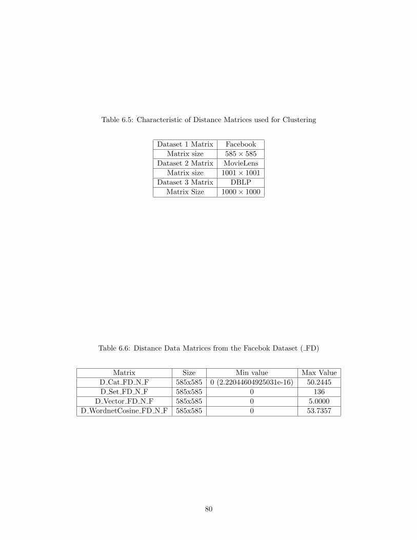
Table 6.5: Characteristic of Distance Matrices used for Clustering
Dataset 1 Matrix Facebook
Matrix size 585× 585
Dataset 2 Matrix MovieLens
Matrix size 1001× 1001
Dataset 3 Matrix DBLP
Matrix Size 1000× 1000
Table 6.6: Distance Data Matrices from the Facebok Dataset ( FD)
Matrix Size Min value Max Value
D Cat FD N F 585x585 0 (2.22044604925031e-16) 50.2445
D Set FD N F 585x585 0 136
D Vector FD N F 585x585 0 5.0000
D WordnetCosine FD N F 585x585 0 53.7357
80
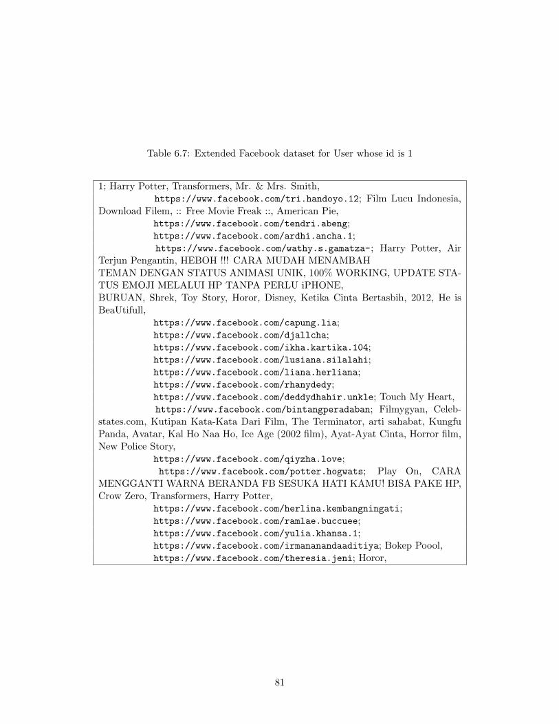
Table 6.7: Extended Facebook dataset for User whose id is 1
1; Harry Potter, Transformers, Mr. & Mrs. Smith,https://www.facebook.com/tri.handoyo.12; Film Lucu Indonesia,
Download Filem, :: Free Movie Freak ::, American Pie,https://www.facebook.com/tendri.abeng;https://www.facebook.com/ardhi.ancha.1;https://www.facebook.com/wathy.s.gamatza-; Harry Potter, Air
Terjun Pengantin, HEBOH !!! CARA MUDAH MENAMBAHTEMAN DENGAN STATUS ANIMASI UNIK, 100% WORKING, UPDATE STA-TUS EMOJI MELALUI HP TANPA PERLU iPHONE,BURUAN, Shrek, Toy Story, Horor, Disney, Ketika Cinta Bertasbih, 2012, He isBeaUtifull,
https://www.facebook.com/capung.lia;https://www.facebook.com/djallcha;https://www.facebook.com/ikha.kartika.104;https://www.facebook.com/lusiana.silalahi;https://www.facebook.com/liana.herliana;https://www.facebook.com/rhanydedy;https://www.facebook.com/deddydhahir.unkle; Touch My Heart,https://www.facebook.com/bintangperadaban; Filmygyan, Celeb-
states.com, Kutipan Kata-Kata Dari Film, The Terminator, arti sahabat, KungfuPanda, Avatar, Kal Ho Naa Ho, Ice Age (2002 film), Ayat-Ayat Cinta, Horror film,New Police Story,
https://www.facebook.com/qiyzha.love;https://www.facebook.com/potter.hogwats; Play On, CARA
MENGGANTI WARNA BERANDA FB SESUKA HATI KAMU! BISA PAKE HP,Crow Zero, Transformers, Harry Potter,
https://www.facebook.com/herlina.kembangningati;https://www.facebook.com/ramlae.buccuee;https://www.facebook.com/yulia.khansa.1;https://www.facebook.com/irmananandaaditiya; Bokep Poool,https://www.facebook.com/theresia.jeni; Horor,
81
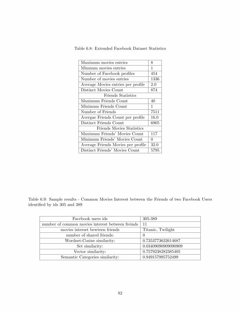
Table 6.8: Extended Facebook Dataset Statistics
Maximum movies entries 8
Minmum movies entries 1
Number of Facebook profiles 454
Number of movies entries 1336
Average Movies entries per profile 2.0
Distinct Movies Count 874
Friends Statistics
Maximum Friends Count 40
Minimum Friends Count 1
Number of Friends 7511
Avergae Friends Count per profile 16.0
Distinct Friends Count 6905
Friends Movies Statistics
Maximum Friends’ Movies Count 117
Minimum Friends’ Movies Count 0
Average Friends Movies per profile 32.0
Distinct Friends’ Movies Count 5795
Table 6.9: Sample results - Common Movies Interest between the Friends of two Facebook Usersidentified by ids 305 and 389
Facebook users ids 305-389
number of common movies interest between freinds 11
movies interset bewteen friends Titanic, Twilight
number of shared friends: 0
Wordnet-Cosine similarity: 0.7353773632614687
Set similarity: 0.03409090909090909
Vector similarity: 0.7579238282385405
Semantic Categories similarity: 0.949157995752499
82
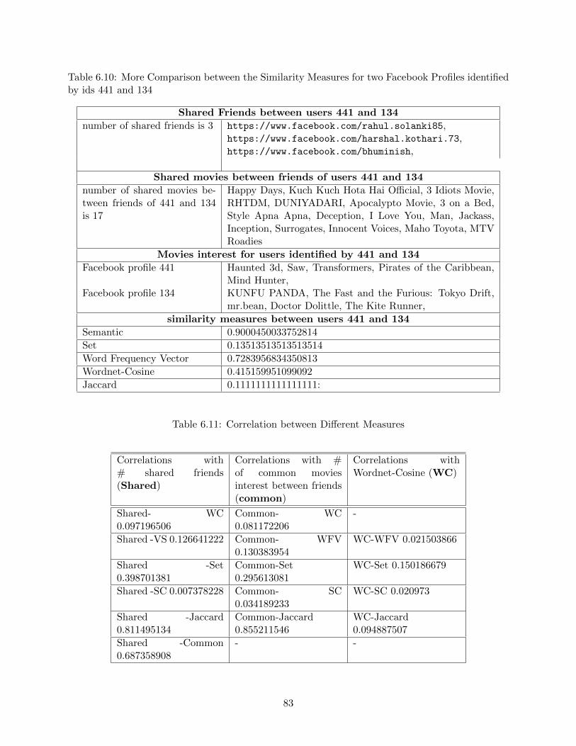
Table 6.10: More Comparison between the Similarity Measures for two Facebook Profiles identifiedby ids 441 and 134
Shared Friends between users 441 and 134
number of shared friends is 3 https://www.facebook.com/rahul.solanki85,https://www.facebook.com/harshal.kothari.73,https://www.facebook.com/bhuminish,
Shared movies between friends of users 441 and 134
number of shared movies be-tween friends of 441 and 134is 17
Happy Days, Kuch Kuch Hota Hai Official, 3 Idiots Movie,RHTDM, DUNIYADARI, Apocalypto Movie, 3 on a Bed,Style Apna Apna, Deception, I Love You, Man, Jackass,Inception, Surrogates, Innocent Voices, Maho Toyota, MTVRoadies
Movies interest for users identified by 441 and 134
Facebook profile 441 Haunted 3d, Saw, Transformers, Pirates of the Caribbean,Mind Hunter,
Facebook profile 134 KUNFU PANDA, The Fast and the Furious: Tokyo Drift,mr.bean, Doctor Dolittle, The Kite Runner,
similarity measures between users 441 and 134
Semantic 0.9000450033752814
Set 0.13513513513513514
Word Frequency Vector 0.7283956834350813
Wordnet-Cosine 0.415159951099092
Jaccard 0.1111111111111111:
Table 6.11: Correlation between Different Measures
Correlations with# shared friends(Shared)
Correlations with #of common moviesinterest between friends(common)
Correlations withWordnet-Cosine (WC)
Shared- WC0.097196506
Common- WC0.081172206
-
Shared -VS 0.126641222 Common- WFV0.130383954
WC-WFV 0.021503866
Shared -Set0.398701381
Common-Set0.295613081
WC-Set 0.150186679
Shared -SC 0.007378228 Common- SC0.034189233
WC-SC 0.020973
Shared -Jaccard0.811495134
Common-Jaccard0.855211546
WC-Jaccard0.094887507
Shared -Common0.687358908
- -
83
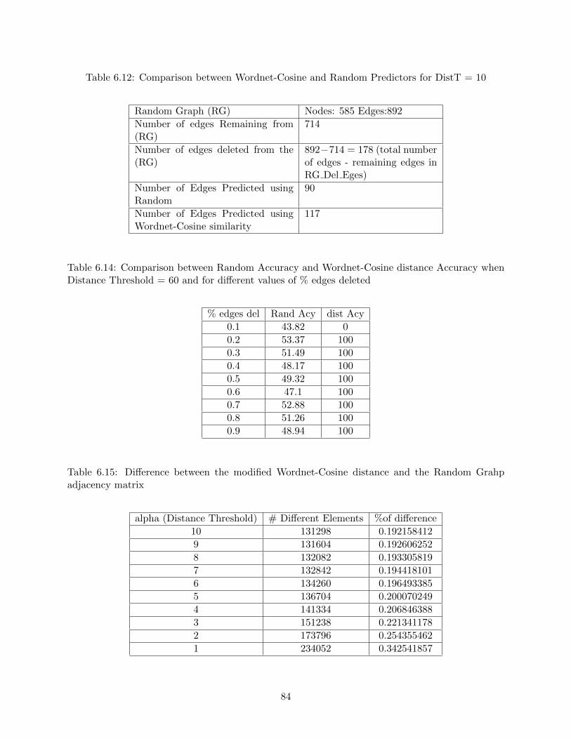
Table 6.12: Comparison between Wordnet-Cosine and Random Predictors for DistT = 10
Random Graph (RG) Nodes: 585 Edges:892
Number of edges Remaining from(RG)
714
Number of edges deleted from the(RG)
892−714 = 178 (total numberof edges - remaining edges inRG Del Eges)
Number of Edges Predicted usingRandom
90
Number of Edges Predicted usingWordnet-Cosine similarity
117
Table 6.14: Comparison between Random Accuracy and Wordnet-Cosine distance Accuracy whenDistance Threshold = 60 and for different values of % edges deleted
% edges del Rand Acy dist Acy
0.1 43.82 0
0.2 53.37 100
0.3 51.49 100
0.4 48.17 100
0.5 49.32 100
0.6 47.1 100
0.7 52.88 100
0.8 51.26 100
0.9 48.94 100
Table 6.15: Difference between the modified Wordnet-Cosine distance and the Random Grahpadjacency matrix
alpha (Distance Threshold) # Different Elements %of difference
10 131298 0.192158412
9 131604 0.192606252
8 132082 0.193305819
7 132842 0.194418101
6 134260 0.196493385
5 136704 0.200070249
4 141334 0.206846388
3 151238 0.221341178
2 173796 0.254355462
1 234052 0.342541857
84
Chapter 7
Conclusion
Finding similarity between profiles in a complex/social network continues to be an issue of great
interest to the network research community. The main approaches to this problem can be divided
into two classes: structural/topological approaches and content/semantic approaches. This thesis
takes as inspiration work in both of these approaches to produce a unified similarity measure,
Wordnet-Cosine, based on a structural approach applied to semantic encoding of profiles. As
its name suggests, Wordnet-Cosine similarity uses Wordnet, a lexical database, to extract and
represent the semantic content of a profile, and combines this with Cosine-similarity, well known
from research in information retrieval.
To illustrate the behavior of Wordnet-Cosine similarity, several experiments have been con-
ducted on three data sets: the Facebook (and extended Facebook), the DBLP, and the Movielens.
The results for the Wordnet-Cosine similarity have shown a relatively more significant performance
over the other similarity measures when applied on one dataset, Movielens, and comparable per-
formance for the other two data sets. When used to predict links the Wordnet-Cosine similarity
outperformed the random method in predicting deleted links from a random social network.
Future Work
The development of, and experiments with Wordnet-Cosine reported in this thesis have opened
up potential new directions in the research of semantic and structural similarity measures for
complex networks. These include (but are not limited to) (1) expanding the second experiment
(link prediction) by using other similarity measure, (2) combine explicitly an edge similarity measure
85
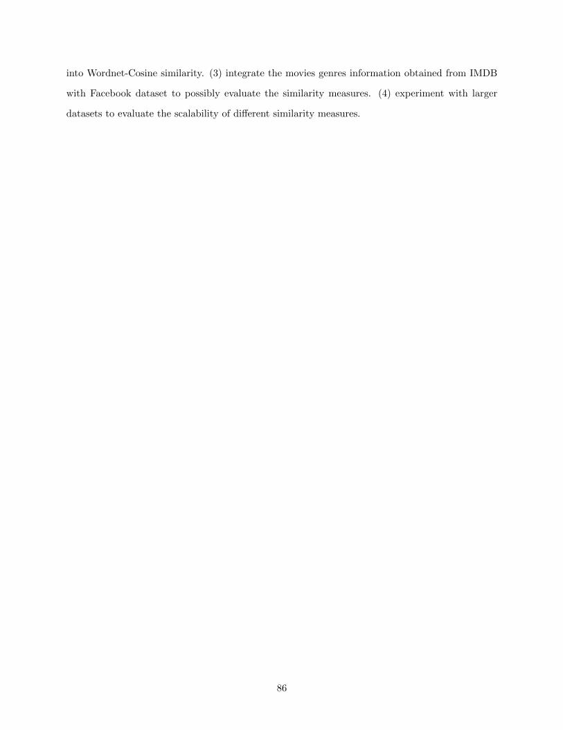
into Wordnet-Cosine similarity. (3) integrate the movies genres information obtained from IMDB
with Facebook dataset to possibly evaluate the similarity measures. (4) experiment with larger
datasets to evaluate the scalability of different similarity measures.
86
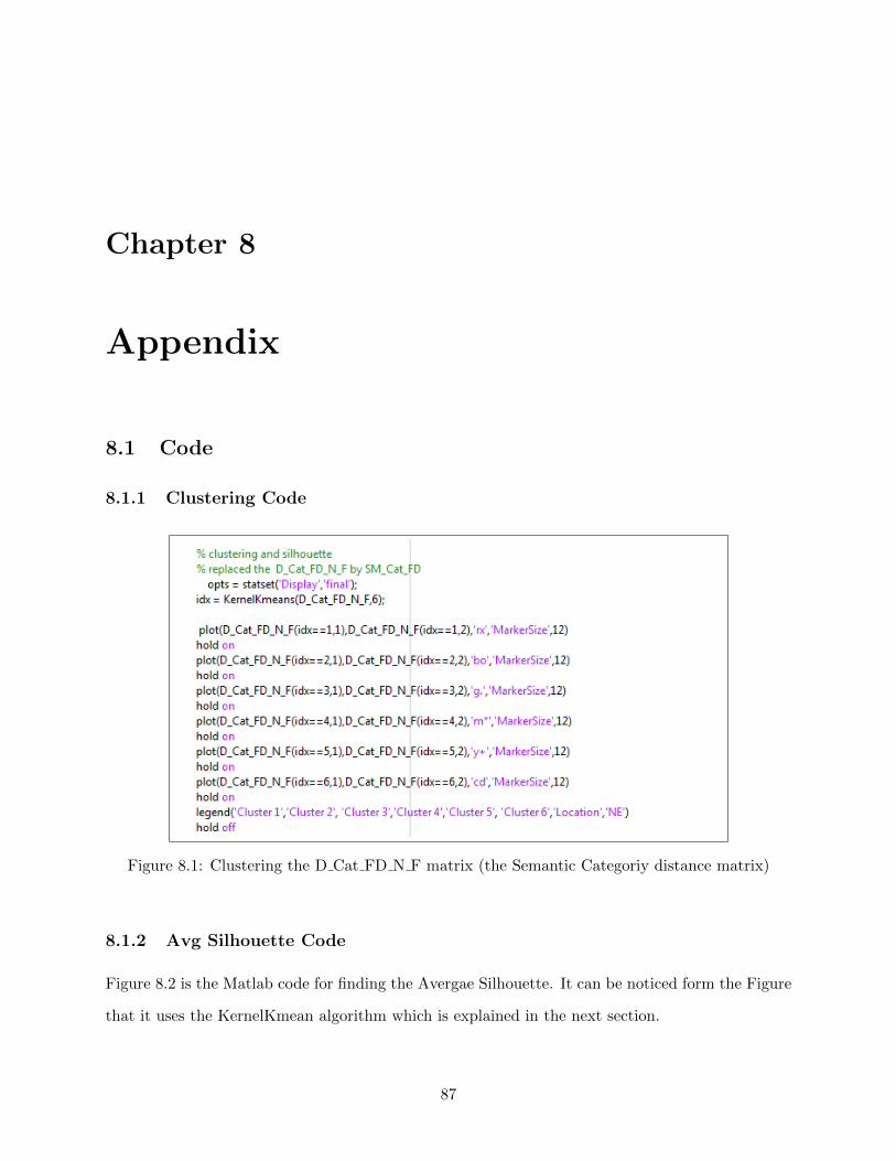
Chapter 8
Appendix
8.1 Code
8.1.1 Clustering Code
Figure 8.1: Clustering the D Cat FD N F matrix (the Semantic Categoriy distance matrix)
8.1.2 Avg Silhouette Code
Figure 8.2 is the Matlab code for finding the Avergae Silhouette. It can be noticed form the Figure
that it uses the KernelKmean algorithm which is explained in the next section.
87
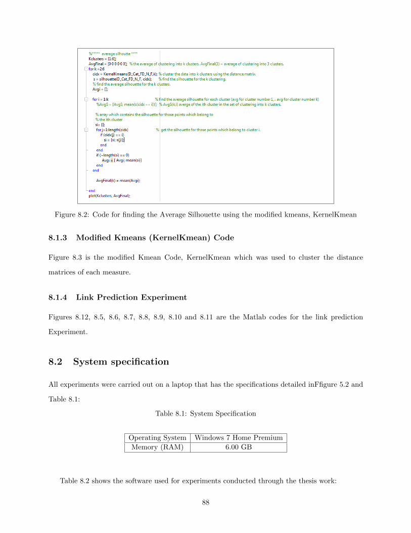
Figure 8.2: Code for finding the Average Silhouette using the modified kmeans, KernelKmean
8.1.3 Modified Kmeans (KernelKmean) Code
Figure 8.3 is the modified Kmean Code, KernelKmean which was used to cluster the distance
matrices of each measure.
8.1.4 Link Prediction Experiment
Figures 8.12, 8.5, 8.6, 8.7, 8.8, 8.9, 8.10 and 8.11 are the Matlab codes for the link prediction
Experiment.
8.2 System specification
All experiments were carried out on a laptop that has the specifications detailed inFfigure 5.2 and
Table 8.1:
Table 8.1: System Specification
Operating System Windows 7 Home Premium
Memory (RAM) 6.00 GB
Table 8.2 shows the software used for experiments conducted through the thesis work:
88
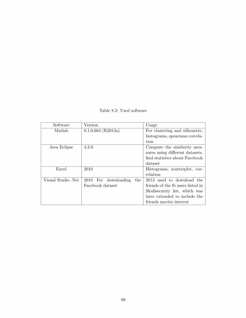
Table 8.2: Used software
Software Version Usage
Matlab 8.1.0.604 (R2013a) For clustering and silhouette,histograms, spearman correla-tion
Java Eclipse 4.2.0 Compute the similarity mea-sures using different datasets,find statistics about Facebookdataset
Excel 2010 Histograms, scatterplot, cor-relation
Visual Studio .Net 2010 For downloading theFacebook dataset
2013 used to download thefriends of the fb users listed inSkullsecurity list, which waslater extended to include thefriends movies interest
89
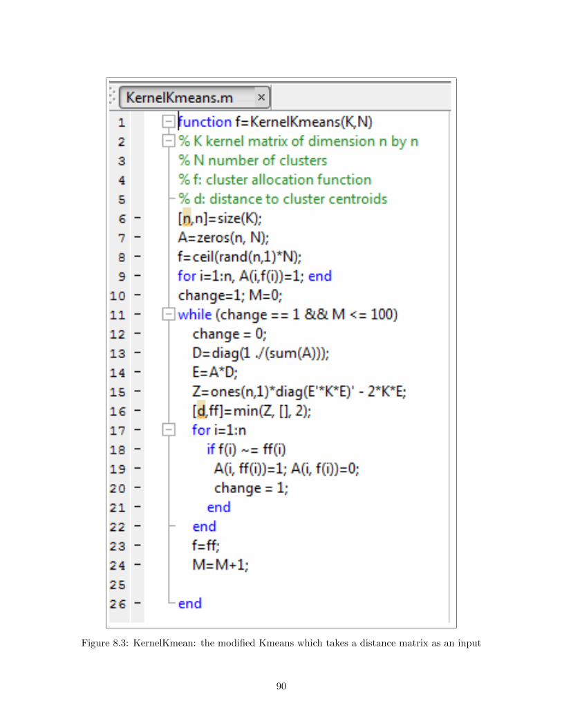
Figure 8.3: KernelKmean: the modified Kmeans which takes a distance matrix as an input
90
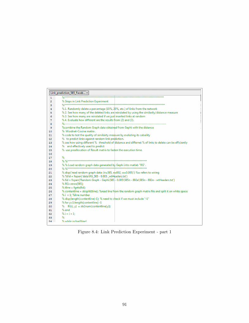
Figure 8.4: Link Prediction Experiment - part 1
91
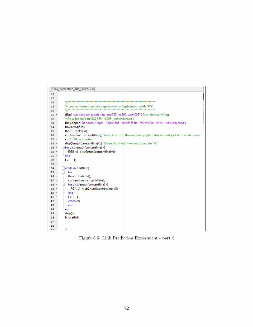
Figure 8.5: Link Prediction Experiment - part 2
92
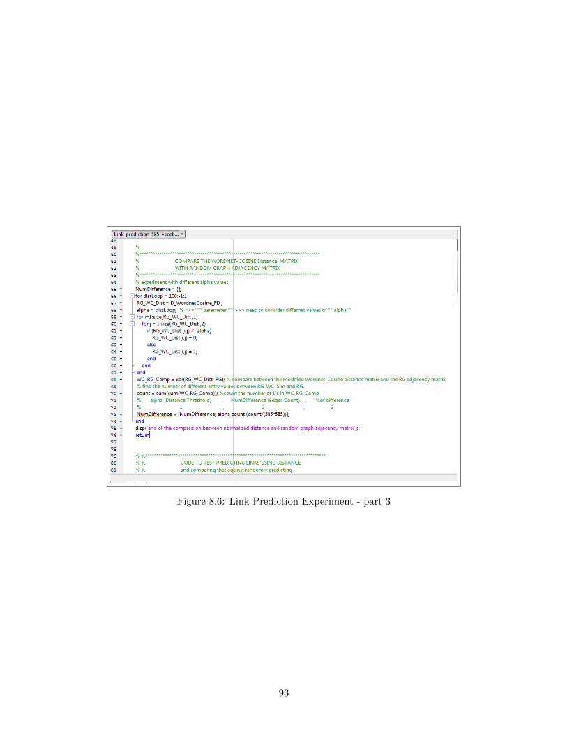
Figure 8.6: Link Prediction Experiment - part 3
93
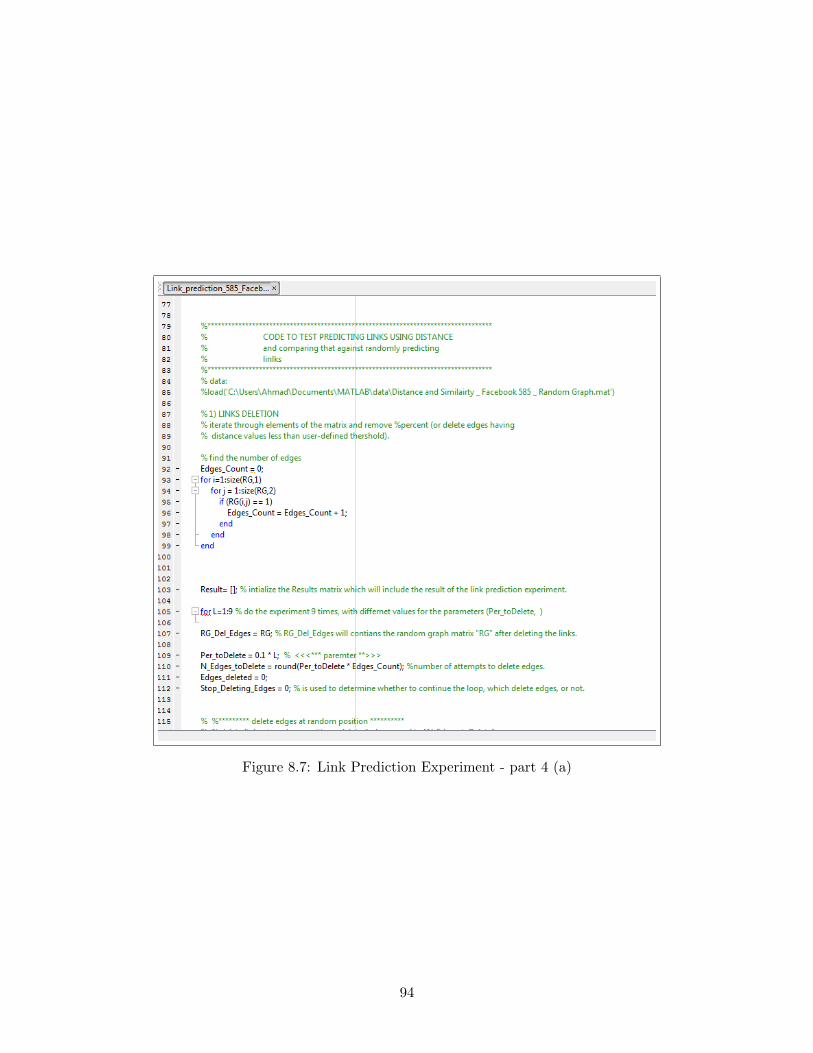
Figure 8.7: Link Prediction Experiment - part 4 (a)
94
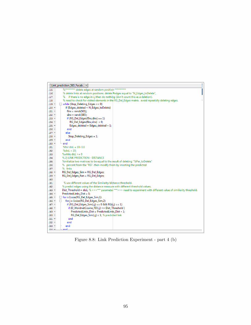
Figure 8.8: Link Prediction Experiment - part 4 (b)
95
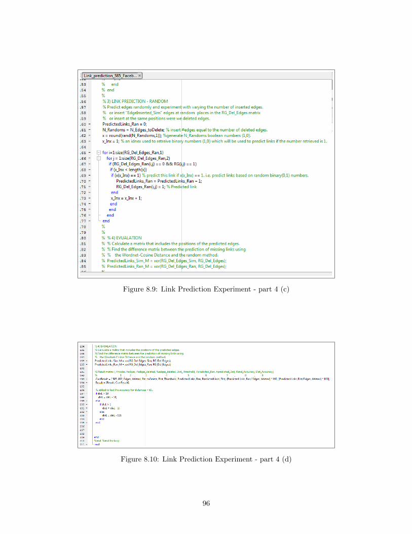
Figure 8.9: Link Prediction Experiment - part 4 (c)
Figure 8.10: Link Prediction Experiment - part 4 (d)
96
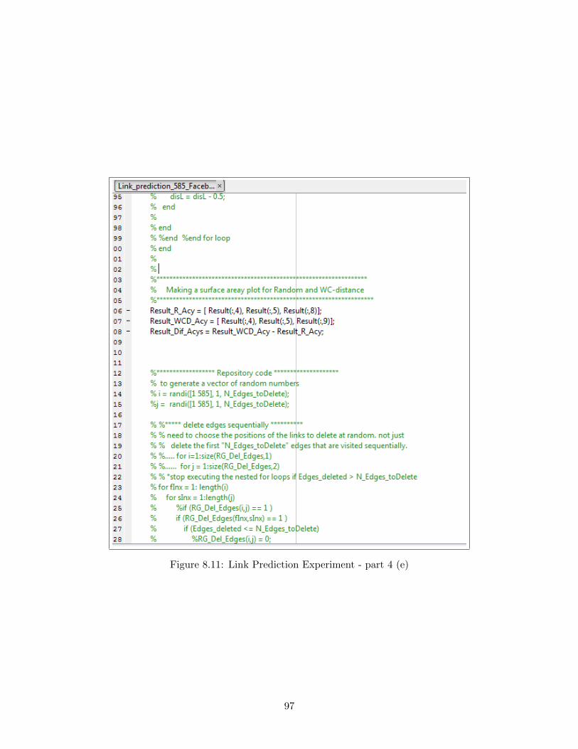
Figure 8.11: Link Prediction Experiment - part 4 (e)
97
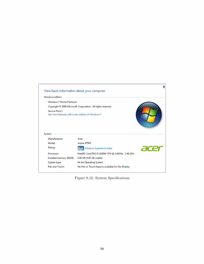
Figure 8.12: System Specifications
98
Bibliography
[1] Cosine Similarity. http://books.google.com/books?id=AyJ9xrrwDnIC&pg=PA50&dq=
cosine+similarity&hl=en&sa=X&ei=mxs6UtatI7G24AOY6YDYDQ&ved=0CDcQ6AEwAQ#v=
onepage&q=cosine%20similarity&f=false.
[2] DBLP dataset. https://snap.stanford.edu/data/com-DBLP.html. [Online; accessed 5-30-
2015].
[3] Stanford Tagger. http://nlp.stanford.edu/software/pos-tagger-faq.shtml. [Online;
accessed 19-July-2014].
[4] Java API for WordNet Searching (JAWS), . http://lyle.smu.edu/~tspell/jaws/index.
html, 2010. [Online; accessed 5-30-2015].
[5] Return of the Facebook Snatchers. http://www.skullsecurity.org/blog/2010/
return-of-the-facebook-snatchers, 2010. [Online; accessed 19-July-2012].
[6] The University of Pennsylvania (Penn) Treebank Tag-set. http://www.comp.leeds.ac.uk/
ccalas/tagsets/upenn.html, 2010. [Online; accessed 19-July-2012].
[7] Lada A Adamic and Eytan Adar. Friends and neighbors on the web. Social networks,
25(3):211–230, 2003.
[8] Cuneyt Gurcan Akcora, Barbara Carminati, and Elena Ferrari. Network and profile based
measures for user similarities on social networks. In Information Reuse and Integration (IRI),
2011 IEEE International Conference on, pages 292–298. IEEE, 2011.
[9] Cuneyt Gurcan Akcora, Barbara Carminati, and Elena Ferrari. User similarities on social
networks. Social Network Analysis and Mining, 3(3):475–495, 2013.
99
[10] Richard D. Juday B. V. K. Vijaya Kumar, Abhijit Mahalanobis. Correlation Pattern Recoog-
nition (page 4). Cambridge, 2005.
[11] Lalit R Bahl, Frederick Jelinek, and Robert Mercer. A maximum likelihood approach to
continuous speech recognition. Pattern Analysis and Machine Intelligence, IEEE Transactions
on, (2):179–190, 1983.
[12] Prantik Bhattacharyya, Ankush Garg, and Shyhtsun Felix Wu. Analysis of user keyword
similarity in online social networks. Social network analysis and mining, 1(3):143–158, 2011.
[13] Prantik Bhattacharyya, Ankush Garg, and Shyhtsun Felix Wu. Analysis of user keyword
similarity in online social networks. Social network analysis and mining, 1(3):143–158, 2011.
[14] Shyam Boriah, Varun Chandola, and Vipin Kumar. Similarity measures for categorical data:
A comparative evaluation. red, 30(2):3, 2008.
[15] Hans-Dieter Burkhard and Michael M Richter. On the notion of similarity in case based
reasoning and fuzzy theory. In Soft computing in case based reasoning, pages 29–45. Springer,
2001.
[16] Hong Cheng, Yang Zhou, and Jeffrey Xu Yu. Clustering large attributed graphs: A balance
between structural and attribute similarities. ACM Transactions on Knowledge Discovery from
Data (TKDD), 5(2):12, 2011.
[17] Seung-Seok Choi, Sung-Hyuk Cha, and Charles C Tappert. A survey of binary similarity and
distance measures. Journal of Systemics, Cybernetics and Informatics, 8(1):43–48, 2010.
[18] Gobinda Chowdhury. Introduction to modern information retrieval. Facet publishing, 2010.
[19] Irene Dıaz and Anca Ralescu. Privacy issues in social networks: a brief survey. In Advances
in Computational Intelligence, pages 509–518. Springer, 2012.
[20] Akilandeswari J Elavarasi, S Anitha and K Menaga. A survey on semantic similarity measure.
International Journal of Research in Advent Technology, 2(4):389–398, 2014.
[21] Nicole B Ellison et al. Social network sites: Definition, history, and scholarship. Journal of
Computer-Mediated Communication, 13(1):210–230, 2007.
100
[22] Facebook. Facebook: 10 years of social networking, in numbers. 2010. [Online; accessed
19-July-2014].
[23] Prasanna Ganesan, Hector Garcia-Molina, and Jennifer Widom. Exploiting hierarchical do-
main structure to compute similarity. ACM Transactions on Information Systems (TOIS),
21(1):64–93, 2003.
[24] John A Hartigan and Manchek A Wong. Algorithm as 136: A k-means clustering algorithm.
Applied statistics, pages 100–108, 1979.
[25] Julia Heidemann, Mathias Klier, and Florian Probst. Online social networks: A survey of a
global phenomenon. Computer Networks, 56(18):3866–3878, 2012.
[26] Xiaodi Huang and Wei Lai. Clustering graphs for visualization via node similarities. Journal
of Visual Languages & Computing, 17(3):225–253, 2006.
[27] P Ilakiya, M. Sumathi, and S. Karthik. A survey on semantic similarity between words in
semantic web. In Radar, Communication and Computing (ICRCC), 2012 International Con-
ference on, pages 213–216. IEEE, 2012.
[28] Paul Jaccard. The distribution of the flora in the alpine zone. 1. New phytologist, 11(2):37–50,
1912.
[29] Glen Jeh and Jennifer Widom. Simrank: a measure of structural-context similarity. In Pro-
ceedings of the eighth ACM SIGKDD international conference on Knowledge discovery and
data mining, pages 538–543. ACM, 2002.
[30] Jay J Jiang and David W Conrath. Semantic similarity based on corpus statistics and lexical
taxonomy. arXiv preprint cmp-lg/9709008, 1997.
[31] EA Leicht, Petter Holme, and Mark EJ Newman. Vertex similarity in networks. Physical
Review E, 73(2):026120, 2006.
[32] Cheng Hua Li, Ju Cheng Yang, and Soon Cheol Park. Text categorization algorithms using
semantic approaches, corpus-based thesaurus and wordnet. Expert Systems with Applications,
39(1):765–772, 2012.
101
[33] Cuiping Li, Jiawei Han, Guoming He, Xin Jin, Yizhou Sun, Yintao Yu, and Tianyi Wu. Fast
computation of simrank for static and dynamic information networks. In Proceedings of the
13th International Conference on Extending Database Technology, pages 465–476. ACM, 2010.
[34] Yuhua Li, Zuhair A Bandar, and David McLean. An approach for measuring semantic sim-
ilarity between words using multiple information sources. Knowledge and Data Engineering,
IEEE Transactions on, 15(4):871–882, 2003.
[35] David Liben-Nowell and Jon Kleinberg. The link-prediction problem for social networks.
Journal of the American society for information science and technology, 58(7):1019–1031, 2007.
[36] Dekang Lin. An information-theoretic definition of similarity. In ICML, volume 98, pages
296–304, 1998.
[37] Zhenjiang Lin, Irwin King, and Michael R Lyu. Pagesim: A novel link-based similarity measure
for the world wide web. In Proceedings of the 2006 IEEE/WIC/ACM International Conference
on Web Intelligence, pages 687–693. IEEE Computer Society, 2006.
[38] Linyuan Lu and Tao Zhou. Link prediction in complex networks: A survey. Physica A:
Statistical Mechanics and its Applications, 390(6):1150–1170, 2011.
[39] Thusitha Mabotuwana, Michael C Lee, and Eric V Cohen-Solal. An ontology-based simi-
larity measure for biomedical data–application to radiology reports. Journal of biomedical
informatics, 46(5):857–868, 2013.
[40] Thusitha Mabotuwana, Michael C Lee, and Eric V Cohen-Solal. An ontology-based simi-
larity measure for biomedical data–application to radiology reports. Journal of biomedical
informatics, 46(5):857–868, 2013.
[41] George A Miller. Wordnet: a lexical database for english. Communications of the ACM,
38(11):39–41, 1995.
[42] Miraj Mohajireen, Charith Ellepola, Madura Perera, Indika Kahanda, and Upulee Kanewala.
Relational similarity model for suggesting friends in online social networks. In Industrial and
Information Systems (ICIIS), 2011 6th IEEE International Conference on, pages 334–339.
IEEE, 2011.
102
[43] Hassan Naderi and Beatrice Rumpler. Three user profile similarity calculation (upsc) meth-
ods and their evaluation. In Signal-Image Technologies and Internet-Based System, 2007.
SITIS’07. Third International IEEE Conference on, pages 239–245. IEEE, 2007.
[44] Ying Pan, De-Hua Li, Jian-Guo Liu, and Jing-Zhang Liang. Detecting community structure in
complex networks via node similarity. Physica A: Statistical Mechanics and its Applications,
389(14):2849–2857, 2010.
[45] Alexis Papadimitriou, Panagiotis Symeonidis, and Yannis Manolopoulos. Fast and accurate
link prediction in social networking systems. Journal of Systems and Software, 85(9):2119–
2132, 2012.
[46] Helen J Peat and Peter Willett. The limitations of term co-occurrence data for query expansion
in document retrieval systems. JASIS, 42(5):378–383, 1991.
[47] Ted Pedersen, Siddharth Patwardhan, and Jason Michelizzi. Wordnet:: Similarity: measuring
the relatedness of concepts. In Demonstration Papers at HLT-NAACL 2004, pages 38–41.
Association for Computational Linguistics, 2004.
[48] Maria S Pera and Yiu-Kai Ng. A group recommender for movies based on content similarity
and popularity. Information Processing & Management, 49(3):673–687, 2013.
[49] Giuseppe Pirro. A semantic similarity metric combining features and intrinsic information
content. Data & Knowledge Engineering, 68(11):1289–1308, 2009.
[50] Ahmad Rawashdeh, Mohammad Rawashdeh, Irene Dıaz, and Anca Ralescu. Measures of
semantic similarity of nodes in a social network. In Information Processing and Management
of Uncertainty in Knowledge-Based Systems, pages 76–85. Springer, 2014.
[51] Peter J Rousseeuw. Silhouettes: a graphical aid to the interpretation and validation of cluster
analysis. Journal of computational and applied mathematics, 20:53–65, 1987.
[52] Henry Small. Co-citation in the scientific literature: A new measure of the relationship between
two documents. Journal of the American Society for information Science, 24(4):265–269, 1973.
103
[53] Matt Spear, Xiaoming Lu, Norman S Matloff, and S Felix Wu. Inter-profile similarity (ips): a
method for semantic analysis of online social networks. In Complex Sciences, pages 320–333.
Springer, 2009.
[54] Ellen Spertus, Mehran Sahami, and Orkut Buyukkokten. Evaluating similarity measures: a
large-scale study in the orkut social network. In Proceedings of the eleventh ACM SIGKDD
international conference on Knowledge discovery in data mining, pages 678–684. ACM, 2005.
[55] Panagiotis Symeonidis, Eleftherios Tiakas, and Yannis Manolopoulos. Transitive node simi-
larity for link prediction in social networks with positive and negative links. In Proceedings of
the fourth ACM conference on Recommender systems, pages 183–190. ACM, 2010.
[56] Kiri Wagstaff. Clustering with missing values: No imputation required. Springer, 2004.
[57] Wensi Xi, Edward A Fox, Weiguo Fan, Benyu Zhang, Zheng Chen, Jun Yan, and Dong Zhuang.
Simfusion: measuring similarity using unified relationship matrix. In Proceedings of the 28th
annual international ACM SIGIR conference on Research and development in information
retrieval, pages 130–137. ACM, 2005.
[58] Ji-Tian Xiao. An efficient web document clustering algorithm for building dynamic similarity
profile in similarity-aware web caching. In Machine Learning and Cybernetics (ICMLC), 2012
International Conference on, volume 4, pages 1268–1273. IEEE, 2012.
[59] Xiao Yang, Zhen Tian, Huayang Cui, and Zhaoxin Zhang. Link prediction on evolving network
using tensor-based node similarity. In Cloud Computing and Intelligent Systems (CCIS), 2012
IEEE 2nd International Conference on, volume 1, pages 154–158. IEEE, 2012.
[60] Xiwang Yang, Yang Guo, Yong Liu, and Harald Steck. A survey of collaborative filtering based
social recommender systems. Computer Communications, 41:1–10, 2014.
[61] Qian-Ming Zhang, Ming-Sheng Shang, Wei Zeng, Yong Chen, and Linyuan Lu. Empirical
comparison of local structural similarity indices for collaborative-filtering-based recommender
systems. Physics Procedia, 3(5):1887–1896, 2010.
104
[62] Peixiang Zhao, Jiawei Han, and Yizhou Sun. P-rank: a comprehensive structural similarity
measure over information networks. In Proceedings of the 18th ACM conference on Information
and knowledge management, pages 553–562. ACM, 2009.
[63] Yang Zhou, Hong Cheng, and Jeffrey Xu Yu. Graph clustering based on structural/attribute
similarities. Proceedings of the VLDB Endowment, 2(1):718–729, 2009.
105