Selling to a Moving Target: Dynamic Marketing Effects in US Presidential Elections

Doug J. Chung Lingling Zhang

Working Paper 15-095

Working Paper 15-095

Copyright © 2015 by Doug J. Chung and Lingling Zhang

Working papers are in draft form. This working paper is distributed for purposes of comment and discussion only. It may not be reproduced without permission of the copyright holder. Copies of working papers are available from the author.

Selling to a Moving Target: Dynamic Marketing Effects in US Presidential Elections

Doug J. Chung Harvard Business School

Lingling Zhang Harvard Business School

1

Selling to a Moving Target:

Dynamic Marketing Effects in US Presidential Elections

Doug J. Chung, Lingling Zhang

Harvard Business School, Harvard University, Boston, MA 02163, United States

dchung@hbs.edu, lzhang@hbs.edu

Abstract

We examine the effects of various political campaign activities on voter preferences in the

domain of US Presidential elections. We construct a comprehensive data set that covers the three

most recent elections, with detailed records of voter preferences at the state-week level over an

election period. We include various types of the most frequently utilized marketing instruments:

two forms of advertising—candidate’s own and outside advertising, and two forms of personal

selling—retail campaigning and field operations. Although effectiveness varies by instrument and

party, among the significant effects we find that a candidate’s own advertising is more effective

than outside advertising, and that campaign advertising works more favorably towards Republican

candidates. In contrast, field operations are more effective for Democratic candidates, primarily

through the get-out-the-vote efforts. We do not find any between-party differences in the

effectiveness of outside advertising. Lastly, we also find a moderate but statistically significant

carryover effect of campaign activities, indicating the presence of dynamics of marketing efforts

over time.

Keywords: multi-channel marketing, personal selling, advertising, political campaigns, dynamic

panel data, instrumental variables.

2

1. Introduction

Choosing the person who stands at the head of a country, guiding its political, social, military,

and economic influence, is inarguably of great importance. Yet the success or failure of electoral

campaigning has long remained a matter of some mystery, explicable—if at all—only after the

dust of a surprising outcome has settled. It is tempting to seek to understand political processes

by applying the principles of the market. After all, isn’t a successful campaign for a presidential

candidate (i.e., convincing more than half the registered voters who actually get to the polls to

cast their ballot as we wish) like making a winning argument that someone should buy a BMW

over a Mercedes? Well, maybe yes—and maybe no.

The most obvious difference is that when the sales figures come in, after the wind-up of

expensive marketing campaigns, BMWs will either have sold better or worse than Mercedes, but

presumably both will have some market share, achieving something and likely surviving through

their hard work and investment. A presidential election, on the other hand, is an extraordinarily

expensive winner-take-all proposition. Second place is quite literally nothing, a complete loss; and

the people working in that “company,” including the CEO-candidate, are in essence then

unemployed.

However, setting aside the differences in stakes and scale between the domains of US national

politics and product marketing, there are striking and informative parallels that allow us to

judiciously apply marketing theory to understand the best and most efficient ways to use the huge

but still finite resources available to a US presidential campaign.

The skyrocketing campaign spending in recent US presidential elections has prompted intense

interest among political strategists, academics, and even the general public in understanding the

effects of political campaigns. For example, in the 2012 Barack Obama versus Mitt Romney

election, the campaigns and their allies spent a total of $2.3 billion, making it the most expensive

US presidential election in history (Sides and Vavreck 2013). Until the 1980s, most academic

studies on political elections concluded that presidential campaigns had only a “minimal effect”:

they simply reinforce a voter’s existing beliefs but are incapable of altering a voter’s political

predisposition or even convincing an intended non-voter to vote (e.g., Finkel 1993, Klapper 1960).

3

In contrast, recent research has come to reach a different conclusion, finding evidence that

campaigns can shift voter preference and hence make a substantial impact on election outcomes.

Yet, several important questions remain unanswered: i) What are the joint effects of various types

of campaign activities such as advertising, candidate live appearances, and field operations? ii)

What are the effects of different types of advertising—a candidate’s own vs. outside advertising?

iii) Do the effects of campaign activities vary by party? And importantly, iv) Are the effects

contemporaneous and largely short-lived, or do they persist? If the latter is true, for how long does

the effect last? Answers to these questions would provide the much-needed insights into guiding

efficient allocation of campaign resources throughout an election period.

Understanding the true campaign effect is a challenging task. One difficulty is related to

measuring voters’ actual exposures to various campaign activities. Many extant papers used

survey-based self-reports, e.g., asking individuals how much media advertising they could recall

being exposed to (Finkel 1993). However, such measures are subject to both the selection bias

(respondents and non-respondents may differ in their levels of interest in politics as well as

attentiveness to campaign activities) and the measurement bias (recall accuracy may correlate

with a voter’s political predisposition) (Goldstein and Ridout 2004). With better empirical data

becoming available recently, several studies have utilized more objective measures on campaign

activities; for example, how much advertising was actually aired in each media market (e.g.,

Gordon and Hartmann 2013, Shaw 1999) and how many field offices were deployed in each county

(Chung and Zhang 2014, Darr and Levendusky 2014).

The second challenge with examining the campaign effects is the endogeneity concern

associated with the level of campaigns. Simply put, how much campaign activities are deployed to

promote a candidate may correlate with how much voter support he or she receives; however, we

researchers may not be able to observe all of the underlying strategic factors, creating an

endogeneity problem. There are at least two reasons why endogeneity may be present in our

context. First, campaign efforts tend to be much more concentrated in the so-called “battleground

states” than in other states simply because, in the present winner-takes-all Electoral College

system, it makes little sense to campaign where the focal candidate is almost surely to win or lose.

4

However, when all candidates shift their strategic emphasis to the battleground states, the head-

on competition there may make the winning margins even narrower in those states than in the

non-battleground states. Second, the changes in campaign activities over time may also be

endogenous. Intuitively, an effective campaign should monitor the voter support to their focal

candidate in each state and promptly adjust the efforts accordingly. Precisely because of these two

reasons, simply correlating the level of campaign activities with voter preferences would yield an

inaccurate estimate of the campaign effect; in some cases we might even identify a negative

association, forced to conclude that campaign activities can actually hurt the candidate.

Extant empirical studies on campaigns have largely acknowledged yet inadequately addressed

the endogeneity concern on campaign planning. The few exceptions include Gordon and Hartmann

(2013) and Huber and Arceneaux (2007), both of which focus exclusively on the effect of campaign

advertising. Gordon and Hartmann (2013) utilized the instrumental variable approach, using

advertising prices in the previous non-election year as instruments for the amount of advertising.

Huber and Arceneaux (2007) exploited a natural experimental setting and examined the effect of

advertising in non-battleground states, where advertising exposures were more “accidental” than

strategic. However, both studies focused on identifying the overall causal effect across elections

and did not address the dynamics of a campaign effect that likely exist within an election period.

The one study that allows for within-election-period dynamics is a paper by Gerber et al.

(2011). By manipulating the level of a gubernatorial candidate’s own advertising in different

media markets through a field experiment, the authors found that political advertising had some

enduring effect over time. Although the field-experimental design offers a clean identification

strategy for causal inference, it comes with a cost of external validity; such experiments are

typically small in scale (both cross-sectional and longitudinal) compared to national presidential

campaigns—Gerber et al. carried out their experiment in roughly 20 media markets for only three

weeks during the 2006 Texas Gubernatorial Election.

While the vast majority of research on political campaigns has addressed mass-media

advertising (e.g., Huber and Arceneaux 2007, Gerber et al. 2011, Gordon and Hartmann 2013), in

reality, candidates have always employed multiple campaign activities—advertising, candidate

5

appearances, field operations—to mobilize and persuade potential voters. Because the levels of

various campaign activities tend to be highly correlated, studying the effect of one without

accounting for the others may lead to an estimation bias. Furthermore, even in the domain of

advertising studies have aggregated candidates’ own and outside advertising into a single variable,

not distinguishing between sources of advertising.1 In addition, as previously mentioned, most past

studies focus on the aggregate campaign effects by utilizing differences across elections rather than

within an election; hence they cannot address one question vital to candidates and campaigns:

how best to allocate resources within an election period. Voter preferences towards a candidate

fluctuate during an election year either because of external shocks or because of the marketing

efforts from the candidate and the rivals. Thus, campaigns are trying to sell their appeal to a

dynamic and moving target.

While earlier studies in this field can probably help provide guidance on how to allocate

campaign resources before the start of the general election, most presidential campaigns have to

deal with ups and downs over an entire campaign period and, thus, need to micro-manage

available resources in a time-specific manner. That is, how much and where to campaign, using

which campaign activities, at which particular time during the election.

In this paper, we examine the dynamic effect of campaigns in the context of US presidential

elections. In particular, we examine all of the principal campaign activities at the disposal of

candidates and their allies, specifically, in the domain of television advertising—both the

candidate’s own and outside advertising—and that of personal selling—the candidate’s live

appearances and field operations. The former involves large-scale mass-media communication

while the latter generates voter contacts in a more targeted and personal manner, analogous to

mass-media advertising and personal selling, respectively, in markets for products and services.

We use multiple sources to compile a comprehensive weekly panel data set at a granular scale

that covers the general-election periods for the 2004, 2008, and 2012 US presidential elections. We

collect detailed records on advertising—both the candidates’ own and outside advertising—and

1 For example, Gordon and Hartmann (2013) aggregates candidates’ own and outside advertising into a single source of advertising. We find significant evidence that the effectiveness differs between these two types of advertising.

6

candidate live appearances during each election period. Furthermore, we measure the scale of field

operations by enumerating the field offices deployed by each party in each state for each of the

three election years.

For our empirical application, we apply the dynamic panel data methods (Arellano and Bond

1991, Arellano and Bover 1995, Blundell and Bond 1998) and treat the campaign variables as

endogenous. Our results generate several insights into understanding the dynamics of campaign

effects. We find both short- and long-term effects for various campaign activities. Although both

candidate’s own advertising and outside advertising boost a candidate’s favorability while

suppressing the rival’s, the former has a much higher marginal impact than the latter. We also

find evidence that field operations boost voter turnout for the focal candidate. Interestingly, a

candidate’s own advertising seems to have a stronger effect for Republican candidates, whereas

the get-out-the-vote effect seems to favor Democratic candidates. The effect of outside advertising

does not seem to vary between parties.

Our paper makes two main contributions. First, using a unique and comprehensive data set,

we generate new insights on the dynamic effect of political campaigns, after addressing both

endogenous campaign planning and heterogeneous voter preferences across candidates and states.

Thus, our results can help political strategists design when, where, how—and how much—to

campaign. Second, our paper jointly estimates the expected payoffs of various campaign activities.

It has more comprehensive coverage on various campaign efforts that are measured at a more

granular level than most extant studies. By including television advertising, candidate appearances,

and field operations, the three most frequently used campaign tools that campaign strategists

employ to influence voter preferences during an election, we comprehensively address the issue of

campaign resource allocation. We elucidate not only the positive effects of a candidate’s own

campaign activities but also the negative effects due to their opponents’ efforts. In particular, this

paper is one of the first attempts to systematically examine the effect of outside political ads, a

force that has gained increasing importance during recent presidential elections. Our finding that

outsides ads behave differently from candidates’ own ads confirms the necessity of separating these

two types of ads when measuring advertising effectiveness and questions the precision of past

7

studies that aggregates these two types of ads into one. In addition, by carefully analyzing the

effect of field operations on voter turnout, our research will inform the effectiveness of the get-out-

the-vote efforts, which have been speculated as one of the factors contributing to Obama’s

landslide victories in the 2008 and 2012 elections.

We believe that our findings will help inform potential presidential candidates and their

political strategists on how best to utilize resources to win an election. There will always be some

external factors that are utterly beyond the control of a candidate or a campaign—acts of

terrorism, financial crises, and natural disasters. Nevertheless, our research will provide guidance

for making the best possible use of the ones that are controllable—the marketing mix variables of

personal selling and mass media advertising.

The remainder of the paper is organized as follows. Section 2 describes the campaign activities

and the data used for empirical analysis. Section 3 presents the model specification and the

empirical estimation strategy. Section 4 discusses the results and section 5 concludes.

2. Data

To properly assess the dynamic effect of campaign activities within an election period, four

pieces of information are essential: (1) voter preferences towards candidates; (2) the amount of

television advertising exposures for the candidates; (3) the schedules of candidate visit

appearances; and (4) the scale of candidates’ campaign field operations. The first three activities

vary both across elections and over time within an election period, while the fourth only varies

across elections. We utilize multiple sources to construct a comprehensive and unique data set

that covers the 2004, 2008, and 2012 presidential elections. Our data structure is a weekly panel

with candidate-state being the cross-sectional units and the data collection period running from

the first week of August to Election Day. Next, we describe each of the data elements in detail.

2.1. Voter preference

Voter favorability for a particular presidential candidate among likely voters is the dependent

variable of interest. We use the actual vote outcomes to measure the final revealed preference of

8

voters. The data are from the CQ Press Voting and Elections Collection, a database that tracks

major US political elections. For each state in each election, we retrieve the votes cast for the

Democratic, the Republican, and the independent candidates. To make the measurement

consistent with the metric used for the periods prior to the Election Day, we calculate, out of the

total number of votes casted, the percentage share of votes received by the Democratic and

Republican candidates, respectively. We then use these shares as the dependent variable in the

last period of each election.

We focus on the more contested or the so-called “battleground states” or “swing states,”

typically the sites of the fiercest battles in presidential elections.2 Residents of battleground states

are exposed to intense campaign advertising on local television networks, repeated candidate visits,

and frequent contacts by field campaign teams; whereas residents of states whose electoral

outcome is a foregone conclusion usually have much less exposure to any type of campaign

activity and, hence, left out of the campaign (Gimpel et al. 2007). The disparate resource

allocation between battleground and non-battleground states is intuitively understandable: it

makes little sense to campaign where the candidate is sure to win or has no chance of winning.

Hence, by focusing only on battleground states, we aim to understand campaign activities where

they matter the most. Therefore, any insights we gain would be all the more relevant for

campaign managers in strategic planning.

Table 1 presents the summary statistics of the actual vote shares in the three elections covered

by our data. Across the battleground states in 2004, the winning candidate, George W. Bush,

acquired an average of 50.0% of the votes while John Kerry acquired 48.9%. In the next two

2 A formal definition of “battleground states,” “swing states” or “contested states” is lacking. Typically, a state is considered a battleground state if no party has an obvious winning margin, based on polls and election results from previous years. We used the list of battleground states defined by Real Clear Politics. In 2004, the battleground states were Arkansas, Arizona, Colorado, Florida, Iowa, Maine, Michigan, Minnesota, Missouri, Nevada, New Hampshire, New Jersey, New Mexico, Ohio, Oregon, Pennsylvania, Washington, West Virginia, and Wisconsin. In 2008, the identified battleground states were Colorado, Florida, Georgia, Indiana, Iowa, Michigan, Minnesota, Mississippi, Missouri, Montana, Nevada, New Hampshire, New Jersey, New Mexico, North Carolina, North Dakota, Ohio, Pennsylvania, South Dakota, Virginia, and Wisconsin. In 2012, the list included Colorado, Florida, Iowa, Michigan, Minnesota, Missouri, Nevada, New Hampshire, North Carolina, Ohio, Oregon, Pennsylvania, Virginia, and Wisconsin.

9

elections, the winning candidate, Barack Obama, received an average of 51.5% and 51.2% in 2008

and 2012, respectively, across the swing states.

<Table 1>

For the weeks leading to Election Day, we measure voter preference (favorability) by the

percent of likely voters who favor the Democratic or the Republican candidate via averaging the

tracking polls conducted by various organizations. Data are acquired from Real Clear Politics

(RCP), a high-quality aggregator of political news and polls. We utilize RCP’s tracking of state-

level poll ratings, which were conducted by a variety of agencies, including polling and consulting

firms such as Gallup and SurveyUSA, as well as newspapers and television channels such as

Washington Post and CNN. The polls vary in sample sizes, with an interquartile range between

580 and 800 likely voters per survey.

As carefully as the political polls were conducted, measurement bias may still persist such that

the poll ratings deviate from the actual voter preference. We do two things to mitigate the impact

of such potential bias. First, in the analysis we use the mean rating averaged over the polls

conducted in the same state during the same time, so that positive and negative biases of

individual ratings cancel out. Second, we exclude partisan polls as they may be subject to a

partisan bias.3 It is known that, in linear regression models, measurement errors in the dependent

variable do not bias the point estimates, as long as they are uncorrelated with the independent

variables or the regression error. This assumption may not hold for partisan polls, as such polls

tend to over-sample partisan voters where the party candidates concentrate their campaign

resources; hence systematic correlations may exist between the measurement errors and the

campaign activity variables. Removing those partisan polls helps curtail the potential bias, to say

the least.4

3 We excluded 20 polls sponsored by Republican-leaning organizations such as Civitas Poll, McLaughlin & Associates, and Moore Information. We also removed 18 polls conducted by the Democratic-leaning groups such as Baydoun/Foster, Democracy Corps, and Public Policy Polling (PPP). 4 The potential measurement errors in our poll ratings could lead to less precision in estimation. In other words, our standard errors are more conservative than they would be in the absence of measurement errors in ratings.

10

We chose to focus on the period beginning in early August, because this is historically

regarded as the starting point of the November general election, when candidates typically start to

carry out full-scale campaign operations. Thus, we end up with 1,507 weekly observations,

covering 19 states for 2004, 21 states for 2008, and 14 states for 2012. Our unit of analysis is

therefore at the state-candidate-week level.

Table 2 presents the summary statistics for the constructed average poll ratings. Note that

the mean poll ratings for the rival candidates were close within each election, confirming intense

competition in the swing states. The poll ratings are interpreted as the average percent of likely

voters who favor a particular candidate. For example, in the 2004 election, across the battleground

states and weeks, an average of 46.6% of the tracking polls of likely voters reported being in favor

of Bush and 46.9% in favor of Kerry.

<Table 2>

It is worth mentioning that tracking polls were much less frequently conducted in non-

battleground states during an election, making the data for those states insufficient for reliable

analysis or inference. Therefore, it makes empirical sense to focus on the battleground states for

our analysis.

2.2. Television advertising

We acquired two types of television advertising data. The first type is advertising made by the

candidates’ own campaigns and their party committees, i.e., the Democratic National Committee

(DNC) or the Republican National Committee (RNC). We refer to this type as “candidate’s own

advertising” or “campaign advertising.” The second type of advertisements is that sponsored by

outside political groups, also known as the Political Action Committees (PACs). These groups can

pull donations from both individuals and organizations, and air television advertising to promote

their favored candidate and attack the rival—under the condition that PACs are prohibited from

coordinating directly with the candidates or their parties. PACs have arguably played a role in US

presidential elections for decades, but they have taken on much greater prominence in the last

several elections, mainly because in 2002 a campaign finance reform law set stricter restrictions on

11

fund-raising and spending; hence, PACs stepped in to fill this gap.5 Especially in the 2012 election,

a relatively new form of organizations—the Super PACs—emerged as major advertisers to spend

heavily on competitive advertising.6 Due to the large number of PACs that advertised in recent

presidential elections, it is challenging to track all the advertisements they sponsored. Fortunately,

we were able to obtain advertising data for the top spenders, which combined were responsible for

more than 90% of the total ad spending made by PACs.

We measure the amount of ad exposure using gross rating points (GRPs), which quantify ad

impressions as a percentage of the target audience reached in an intended market. For example, if

an advertisement aired in the Des Moines-Ames area reached 25% of the target population, it

received a GRP value of 25; if the same advertisement was aired ten times, the GRP value would

be 250 (= 25 × 10). Thus, 250% of the target audience was exposed to advertisement; or

equivalently, a representative person in the market viewed the ad 2.5 times. GRPs are a more

accurate measure of ad exposure than dollar spending is, because the prices of advertising vary

significantly across markets. For example, the same amount of ad dollars would yield much less

exposure in Los Angeles than in Kansas City. Hence, GRPs provide a measure of audience

exposure independent of cost.

We obtained advertising data from Nielsen Media Research, which divides the US media

market into 210 designated market areas (DMA): residents throughout one DMA receive largely

the same television offerings including advertising. Therefore, our advertising metrics were

originally collected at the DMA level. To match advertising to the states, we construct state-level

ad exposures by taking the weighted average of DMA-level GRPs across the DMAs from the same

state. For instance, in Colorado there are four overlapping DMAs: Albuquerque-Santa Fe,

Colorado Springs-Pueblo, Denver, and Grand Junction-Montrose. For each DMA, we calculate a

weight variable that equals the percentage of Voting Age Population (VAP, i.e., resident citizens

5 The Bipartisan Campaign Reform Act of 2002, enacted on March 27, 2012, regulates the financing of political campaigns in the U.S.—Source: http://en.wikipedia.org/wiki/Bipartisan_Campaign_Reform_Act, retrieved May 22, 2015. 6 Super PACs are made up of independent PACs that support a candidate with unlimited—and often anonymous—donations from unions, companies, or individuals.

12

aged 18 and above) who live in the focal DMA out of the total Colorado Voting Age Population.7

After the weight is assigned to each DMA-Colorado pair, the GRPs for Colorado is defined as the

weighted average of DMA-level GRPs across those four overlapping DMAs. In summary, the total

advertising exposure for candidate i in state s at time t would be

1

sD

ist d idtd

a w a=

= å

where Ds is the number of overlapping DMAs, wd is the population weights, and aidt is the GRPs

for candidate i in DMA d during week t.

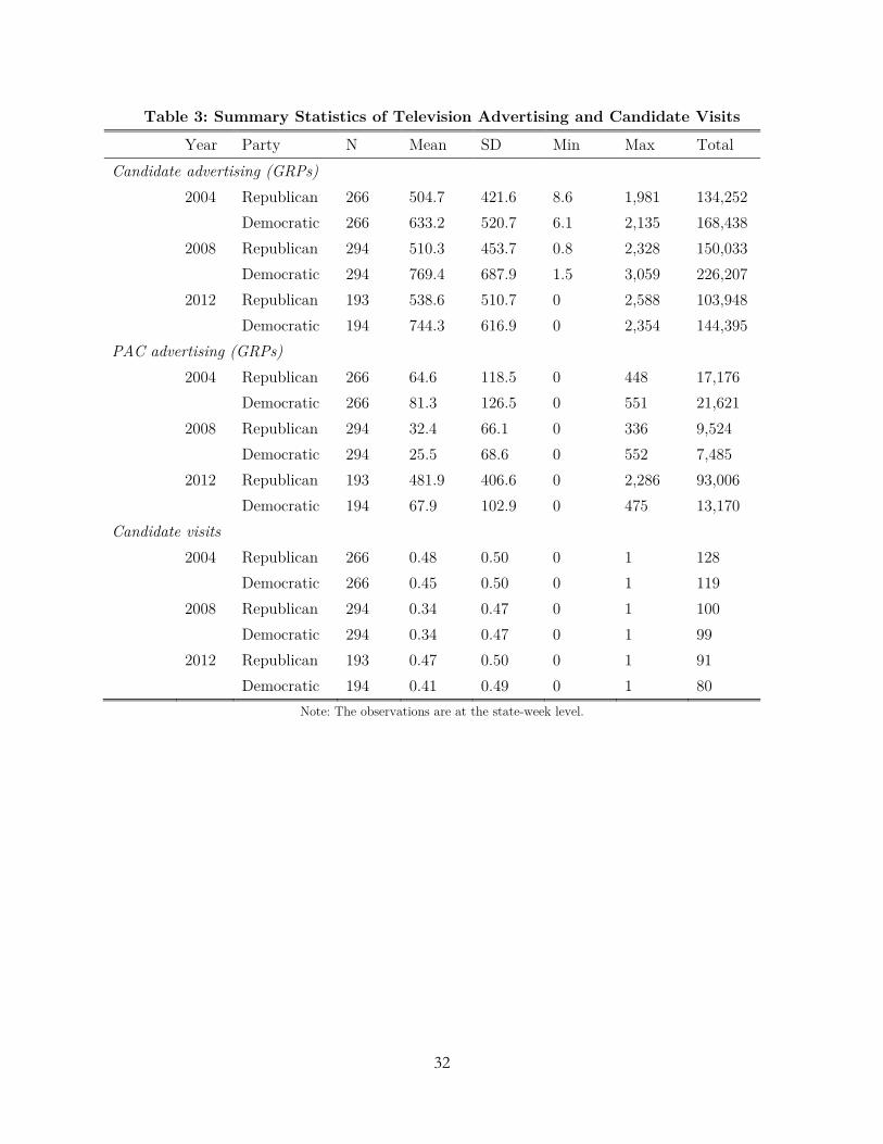
The summary statistics for advertising are presented in Table 3. Across the battleground

states, the Democratic candidates had more advertising than the Republicans in all three elections:

on average, ad impressions from the Democratic candidates were higher by 25%, 51%, and 39% in

2004, 2008, and 2012, respectively. The Democrats also received more outside PAC ads in 2004,

but had fewer than the Republicans in the next two elections. Overall, the Republican candidates

received 27% more outside ads in 2008 and a whopping 606% more in the 2012 election. When we

combine the ads sponsored by the candidate’s campaign with those sponsored by the PACs, we

see that overall the Democratic candidates had more ad impressions in 2004 and 2008. However,

in the 2012 election, ads from the PACs supporting Romney significantly outweighed the outside

ads supporting Obama; in the end, the Romney candidacy had 25% more ad impressions in the

battleground states than Obama.

<Table 3>

To examine how advertising evolves within a single election, we plot for each year the total ad

GRPs aired by the candidates and their party committees in Figure 1. There is a clear rising trend

of ad intensity as Election Day approaches. For example, in 2004, the Democratic candidates and

party committee bought 3.7 times as many GRPs in the last five weeks of the election as it did in

the first five weeks (beginning August 1). This ratio was 5.6 and 2.9 for 2008 and 2012,

7 A DMA can cross multiple state lines. Take DMA “Albuquerque-Santa Fe” for example. It consists of one county from Arizona, four from Colorado, and twenty-seven from New Mexico. When calculating the VAP-weight variable for the Albuquerque-Santa Fe-Colorado pair, we divided the sum of VAP from the four Colorado counties by the total Colorado VAP.

13

respectively. The within-campaign increase in ad impressions is similar for the Republicans, with

the ratios being 3.3, 3.6, and 2.9, for the three elections respectively.

<Figure 1>

Figure 2 depicts the total GRPs per week for PAC ads. It is noteworthy that the PACs

increased their spending in 2012 by a significant amount compared with the 2004 and 2008

presidential elections so that the three panels in Figure 2 required different scales for the y-axis.

We do not observe obvious trends for 2004 and 2008, but see a similarly rising pattern for 2012

when the PAC ad spending was much more substantial.

<Figure 2>

2.3. Candidate appearances

In addition to television advertising, candidates also carry out on-the-ground campaigns by

visiting battleground states for face-to-face contacts with voters. Candidates hold town-hall

meetings, attend rallies, host fund-raising events, and sometimes make impromptu stops to simply

shake hands with supporters. This is usually referred to as “retail politics” (Vavreck et al. 2002),

in the sense that candidates seek to personally target and influence voters on a small and local

scale. Such live appearances also generate free media coverage that may reach local residents who

do not physically attend campaign rallies. We measure retail campaigning by finding out whether

the presidential or vice-presidential candidates made a campaign-related appearance in a

particular state during each week. The visit schedules were collected from the “Democracy in

Action” project hosted by George Washington University. The project maintains detailed records

of where and how the candidates spent their time during the fall campaign of most recent

presidential elections. The information is based on travel announcements provided by the

campaign teams, supplemented with records of news accounts.

Summary statistics of candidate appearances are reported at the bottom of Table 3. For two

elections, the Republican candidates made more frequent visits to the battleground states. In the

2004 election, 48% of the state-week observations had a visit appearance from the Republican

candidates compared with 45% from the Democrats. In 2012, the numbers were 47% versus 41%.

In contrast, we see no differences between the parties for the 2008 election.

14

2.4. Field operations

In recent presidential elections, grassroots mobilization activities have seen a strong resurgence

among the mix of important campaign techniques available to candidates (Darr and Levendusky

2014, Masket 2009). Campaigns increasingly rely on ground operations to mobilize potential voters

and encourage get-out-the-vote efforts. Often referred to as the “ground game” (in contrast to

advertising on the airwaves), those grassroots activities enable the campaign to make direct voter

contacts but at a much larger scale than retail campaigning. The vast majority of direct voter

outreach—such as door-to-door canvassing or talking to voters in supermarket parking lots—is

coordinated through campaign field offices. Therefore, we use the number of field offices per state

to measure the scale of campaign field operations.

Table 4 presents the summary statistics for field operations. Throughout all three elections

under study, the Democratic candidates deployed many more field offices in battleground states

than Republicans did. Among the Democratic candidates, Obama clearly placed an even stronger

emphasis on field operations than Kerry. In 2008, his campaign had more than 70 field offices in

Ohio and Virginia; and in 2014, had the largest number of field offices in Florida and Ohio.

It should be noted that the raw number of field offices may not represent the true “effective

reach” of field operations: the effect of an office may depend on the size of the population it

targets. For example, the effective reach—e.g., the percent of target population reached as in

GRP—for a field office in New Hampshire may be much higher than that in Florida, simply

because the latter is much more populated. Therefore, we normalize the number of field offices by

the inverse of the VAP for each state. The new metric is the number of field offices per 100,000

VAP (see the bottom section of Table 4 for the summary statistics). Taking the population size

into account, we see that the Republican candidates consistently deployed roughly 0.2 to 0.4 field

offices per 100,000 VAP across the three elections, while the Democratic candidates had a much

greater number. Between the Democratic candidates, Obama’s scale of field operations roughly

doubled Kerry’s (Obama had roughly 1.0 field office per 100,000 VAP in 2008 and 2012 and Kerry

had 0.5). The VAP-normalized field operations are used in our analysis.

< Table 4>

15

2.5. Model-free evidence

In this section we present some model-free evidence on the relation between advertising and

voter preferences. To control for cross-sectional differences across states, we examine the

association between the weekly changes in advertising and the corresponding changes in poll

ratings. We illustrate candidate advertising in Figure 3 and PAC advertising in Figure 4.

Figures 3a and 3b show scatter plots of the percentage change in a candidate’s own

advertising and that of his rival, respectively, along with the percentage change in poll ratings and

the best-fitting nonparametric smoothed polynomial with its 95-percent confidence interval shaded

in gray. Thus, for Figure 3a, the horizontal axis is the percentage change of candidate i’s

advertising in state s from week t-1 to t, i.e., , , 1 , 1100 ( ) /c c cis t is t is ta a a- -´ - , and the vertical axis

corresponds to the percentage change in poll ratings, i.e., , , 1 , 1100 ( ) /is t is t is ty y y- -´ - . Overall, we

see a positive trend, suggesting that voter preference towards a candidate tends to rise with an

increase in advertising intensity. In Figure 3b, we illustrate the rating changes against the changes

in ad exposures from the rival candidates. As expected, the more a competitor advertises, the

lower the focal candidate’s poll ratings. Thus, the positive own-ad effect and the negative

competitive-ad effect provide initial evidence that candidate advertising seems to be effective in

shifting voter preferences.

< Figure 3 >

Figure 4 depicts the relation between PAC advertising and voter preferences. Figure 4a shows

PAC ads that support the focal candidate and Figure 4b presents ads in favor of the rival

candidate. Again, the plot exhibits a positive own-ad effect: more PAC ads for the focal

candidates are in general associated with more favorable ratings, and vice versa. However, the

scatterplot does not show an obvious relation between poll favorability and PAC ads in support of

the rival candidates.

< Figure 4 >

To gain an initial understanding of the dynamics (or persistence) of the ad effect, we plot the

changes in poll ratings against the lagged changes in advertising, that is, the percentage GRP

16

change in the previous weeks. The top two panels in Figure 5 are for the candidate’s own ads and

the bottom two are for the PAC ads in support of the focal candidate. We find a positive

association between ratings and advertising from the previous week (Figures 5a and 5c),

suggesting that the ad effect may persist for at least a week. However, with a lag of two weeks,

the pattern is mixed. We see a negative trend for the candidate’s own ads (Figure 5b) but a weak

positive trend for PAC ads (Figure 5d). Therefore, Figure 5 does not provide sufficient evidence

for whether the effect of advertising lasts more than one week.

< Figure 5 >

It is noteworthy that Figures 3 through 5 do not account for the possible endogeneity issue

mentioned previously with regards to campaign activities. That is, candidates and PACs can

increase advertising in anticipation of declining favorability ratings and decrease them in the

opposite situation. If such a “balancing” effect is at work, tracking poll ratings could seem

unchanged despite changes in advertising, whereas, in the case of declining favorability, campaigns

could have prevented the ratings from dropping further. To assess the true causal effect of

advertising (and other campaign activities as well), we need a formal model that carefully

addresses endogeneity; we present our modeling approach in the next section.

3. Model

3.1. Dynamic Model

Let yist be the voter preference for candidate i across residents in state s at week t. Naturally,

yist would be a function of the previous week’s voter preference yis,t-1, and current campaign

activities. The activities include candidate i’s own campaign activities and those by i’s rivals (-i),

as well as the mobilization and persuasion efforts sponsored by PAC groups. We also allow yist to

be a function of unobservable factors related to candidates, states, and time. Formally, we model

candidate preference (favorability) ratings in the following multiplicative specification:

( ) ( ) ( ) ( ) ( ) ( )1 2 1 2

, 1 ( ) ( ) 1 2 ( )expc c o oist is t ist i st ist i st ist i st t ist is t isty y a a a a R R I F

d d h hlj j b a g e- - - -= + + + + + … (1),

17

where l is the carryover factor that measures how much of previous week’s voter preference

persists to the current week; cista , o

ista , and istR are the candidate’s own advertising, outside PAC

advertising supporting candidate i, and the candidate’s campaign appearances in state s during

week t, respectively; ( )c

i sta- , ( )o

i sta - , and ( )i stR- are the corresponding campaign activities from the

rival party; d, h, and j are the marginal effect for candidate advertising, PAC advertising, and

retail campaigning, respectively, where subscript 1 corresponds to the own effect and subscript 2

the competitive effect; ais is the candidate-state specific effect that accounts for the time-invariant

favorability towards candidate i for residents in state s; gt captures the weekly shocks to voter

preference that are common to candidates and states; and eist is the idiosyncratic shock specific to

each candidate, state, and week combination. Lastly, It is an indicator variable that equals one if t

is the Election week and zero otherwise, Fist is the intensity of field operations deployed by

candidate i in state s, and b is the corresponding marginal effect of field operations; therefore, by

utilizing the difference between the final poll results and the actual outcome of the election,

t istI Fb captures the systematic effect of field operations on voter turnout.

We model voter preference in a multiplicative functional form to allow for non-linear effects of

campaign activities. The clear advantage of this specification becomes apparent after we take the

logarithm transformation on the two sides of equation (1), yielding the following equation used for

estimation:

, 1 1 2 ( ) 1 2 ( ) 1 2 ( )c c o o

ist is t ist i st ist i st ist i st t ist is t istY Y A A A A R R I Fl d d h h j j b a g e- - - -= + + + + + + + + + + … (2)

where log( )ist istY y= and log( )ist istA a= .

In any attempt to predict voter preference for presidential candidates, it is critical to take into

account not only the campaign activities but also the contextual factors that may shape voter

preferences. Campbell (1992) proposed two sets of such variables, the first of which indicates the

national political climate that functions as background for the current campaigns and includes

factors such as the incumbency status of the presidential candidates and the state of the national

economy. The second set, composed of characteristics of the states, includes variables like the

18

home-state advantage for the presidential and vice-presidential candidates, and the rate of

economic growth in each state. We capture all of these effects using the candidate-state fixed

effect ais, which also absorbs the impacts from any other unobservable nation-wide or state-level

factors, as long as the effect is time-invariant throughout the weeks of the general election.

The weekly shifts in voter preference are captured by the week fixed effect gt, which measures

the shocks that vary over time but are homogenous across candidates and states. One example is

the fact that voters tend to be more interested in candidates as Election Day approaches; in this

case, gt would capture any common contemporaneous fluctuations in voter preference. Including

the weekly fixed effects also helps remove the interdependence among the cross-sectional units, as

failure to do so may introduce autocorrelation among eist and, thus, violate the zero serial

correlation assumption required for estimation, which we will explain in the estimation section.

It is worth noting that because Obama was a candidate in two of the three elections, we treat

his candidacy in 2008 and 2012 as two separate cross-sectional units. Thus, ais allows varying

levels of preference towards him in the same state between the two elections.

3.2. Estimation

The specification in the form of equation (2) allows the distinction between the short-run

dynamics and the long-run relationship, but calls for careful estimation. First, by construction, the

lag of the dependent variable on the right-hand side of the equation, Yis,t-1, is correlated with the

unobserved candidate-state fixed effect, ais. Because of this endogeneity concern, the ordinary

least square (OLS) regression would generate biased estimates, referred to as the dynamic panel

bias (Nickell 1981). One possible approach to mitigate this problem would be to include dummy

variables for each candidate-state combination and perform the so-called least-squares dummy-

variable (LSDV) regression, which is equivalent to eliminating the mean differences across

candidate-states and obtaining the within-group fixed-effect (FE) estimator.8 However, in dynamic

8 The FE estimator generates biased standard errors because it does not take into account the loss in degrees of freedom due to the mean transformation.

19

panel data, the within-group estimator does not eliminate the dynamic panel bias (Nickell 1981):

after the de-meaning transformation, the new lagged dependent variable *, 1 , 1is t is t isY Y Y- -= - would

still be correlated with the new error term *ist ist ise e e= - because , 1is tY - in *

, 1is tY - is negatively

correlated with eis,t-1 in *iste . Interestingly, in OLS, the lagged variable Yis,t-1 and the error term

( is ista e+ ) are positively correlated. Thus, the OLS and the LSDV estimators provide the upper

and lower bounds for the range of the true parameter value for the carryover factor l (Bond 2002);

hence, we first perform the OLS and the LSDV regression to generate benchmark values for the

carryover factor.

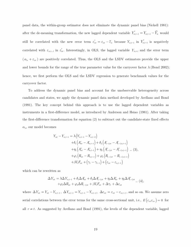
To address the dynamic panel bias and account for the unobservable heterogeneity across

candidates and states, we apply the dynamic panel data method developed by Arellano and Bond

(1991). The key concept behind this approach is to use the lagged dependent variables as

instruments in a first-difference model, as introduced by Anderson and Hsiao (1981). After taking

the first-difference transformation for equation (2) to subtract out the candidate-state fixed effects

ais, our model becomes

( )( ) ( )( ) ( )( ) ( )

( ) ( )

, 1 , 1 , 2

1 , 1 2 ( ) ( ) , 1

1 , 1 2 ( ) ( ) , 1

1 , 1 2 ( ) ( ) , 1

1 , 1

ist is t is t is t

c c c cist is t i st i s t

o o o oist is t i st i s t

ist is t i st i s t

t ist t t ist is t

Y Y Y Y

A A A A

A A A A

R R R R

I F

l

d d

h h

j j

b g g e e

- - -

- - - -

- - - -

- - - -

- -

- = -

+ - + -

+ - + -

+ - + -

+ + - + -

… (3),

which can be rewritten as

, 1 1 2 ( ) 1 2 ( )

1 2 ( )

c c o oist is t ist i st ist i st

ist i st t ist t ist

Y Y A A A AR R I F

l d d h h

j j b g e- - -

-

D = D + D + D + D + D

+ D + D + +D +D… (4),

where , 1ist ist is tY Y Y -D = - , , 1 , 1 , 2is t is t is tY Y Y- - -D = - , , 1ist ist is te e e -D = - , and so on. We assume zero

serial correlations between the error terms for the same cross-sectional unit, i.e., ( ) 0ist isrE e e = for

all r t¹ . As suggested by Arellano and Bond (1991), the levels of the dependent variable, lagged

20

two periods or more, are valid instruments in the equation in first differences. We form the

identification restriction as

( ), 0is t q istE Y e- D = … (5),

where 2,3,...,( 1)q t= - and 3, 4,...,t T= , and can use the generalized method of moments (GMM)

(Hansen 1982, Wooldridge 2002) to estimate our parameters of interest.

This estimator may perform poorly if Yist is close to a random walk, so that the past levels

(the instruments) convey little information about future changes (the lagged differences). To

improve efficiency, Arellano and Bover (1995) and Blundell and Bond (1998) further suggested the

use of lagged differences of Yist as instruments for the equation in levels. The identification

restriction is expressed as

( ), 1 0ist is tE Yu -D = … (6),

for 3,4,...,t T= , where ist is istu a e= + . Such instruments are valid as long as the changes in

voter preference are uncorrelated with the fixed effect: ( ) 0is istYE a D = for all i, s, and t. Using

this additional set of instruments would require stacking the equations in differences and the

equations in levels for periods 3, 4, …, T ; hence, this is typically referred to as the System GMM

estimator.

We have completed the specification of the instruments necessary to identify the carryover

factor l. However, we also need to consider instruments to identify the effect of campaign

activities, which we have good reasons to believe are endogenous. During the general election,

candidates and their campaign teams closely monitor any fluctuations in voter favorability in

battleground states, taking prompt actions to boost goodwill or reduce damages from negative

news. For example, in September 2012, the Obama campaign launched television ads attacking

Romney’s November 2008 New York Times article, “Let Detroit Go Bankrupt,” and asserted that

Romney actually profited from the auto bailout. Such ads were a blow to the Romney candidacy,

21

especially in Rust Belt states like Ohio.9 The impact of events like these would be captured by eist

as a negative shock in our model. Shortly after the ads were aired, the Romney campaign went

into a crisis-management mode to reduce the damage, more intensively in Michigan and Ohio,

where voters’ goodwill was perhaps damaged the most. Of course, this is only one of the many

examples of why campaign activities may be correlated with idiosyncratic shocks: ( ) 0ist istE M e ¹

for all t, where istM represents cistA , ( )

ci stA- , o

istA , ( )o

i stA- , istR , and ( )i stR- .

We again exploit the panel structure of the data to construct instrumental variables to address

the endogeneity concern regarding campaign activities. The argument behind the instruments for

istM is similar to that for the lagged dependent variable. In a nutshell, we use the lagged variables

as instruments for differences and the lagged differences as instruments for levels. The

identification restriction is written as

( ), 1 0ist is tE Mu -D = ; ( ), 0is t q istE M e- D = … (7),

where 2,..., 1q t= - .

Similar to the time-varying campaign activities Mist, one can argue that the intensity of field

operations is also endogenous and so our estimates of the parameter b would be biased. By having

an extensive set of candidate-state fixed effects, we help mitigate the endogeneity problem

associated with field operations. Nevertheless, to address this possible endogeneity problem, we use

real estate rental prices in the previous non-election year to instrument field operations. The logic

is similar to that behind the use of cost shifters to instrument prices in the traditional marketing

and economics literature. That is, the previous year’s real estate rental price in a state is

exogenously determined outside our model specification—specifically, exogenous with regards to

election-specific shocks—but it should be correlated with the current year’s rental price, which

shifts a candidate’s choice to deploy field operations in that state. We use the rental price from

the previous year instead of the current year, because the latter may be affected by the changing

demand of office space due to election-related activities, and hence may not be a valid instrument.

9 The Wall Street Journal, February 23, 2012, from http://blogs.wsj.com/washwire/2012/02/23/obama-super-pac-air-ads-in-michigan-on-auto-bailout.

22

Along with using real estate rental prices to instrument the intensity of field operations, we

combine the restriction conditions of (5), (6), and (7) to form an estimator with endogenous

predictors. The parameter estimates and the standard errors follow the GMM estimation

procedures.

4. Results

We first perform OLS and LSDV estimations of equation (2) and report the parameter

estimates in Table 5. Columns (1) and (2) correspond to the OLS and LSDV estimators,

respectively. The carryover parameter is estimated to be high, 0.756 (p<0.01), in the OLS pooled

regression. This is expected, as the association between the lagged and the contemporaneous voter

preference would be inflated when the candidate-state fixed effects are not accounted for. After

including the candidate-state fixed effects, the carryover parameter estimate drops to 0.288

(p<0.01) in the LSDV regression. As mentioned previously, these two values provide the lower

and upper bounds for the true value of the carryover parameter.

<Table 5>

We present the results of our model using moment conditions in equations (5), (6), and (7).

Our final model is based on equation (2) but further allows the campaign effect to vary by parties

by including the interactions between a Democratic indicator and the campaign activity

variables.10

Furthermore, although all of the lags— ,is t qY - and ,is t qM - for 2,3,...,( 1)q t= - —are valid

instruments in the difference equations, we have to be careful with choosing the number of

instruments. Too many lags lead to estimating a large variance-covariance matrix, which may be

challenging for a finite sample like ours (Roodman 2009). As a result, we retain a selected range of

lags to make sure that the variance-covariance matrix is of a reasonable size.11 In particular, we

estimate the model using three alternative lag specifications, and report the parameter estimates

10 We used Stata’s command xtabond2 (Roodman 2009) to estimate the parameters. 11 In addition to limiting the number of lags, we collapse the matrix of instruments for our endogenous campaign variables such that the number of instruments is of a reasonable size. We use the collapse option in the Stata command xtabond2.

23

and the number of instruments for each specification. The instruments in column (1) are variables

lagged two-to-three periods, column (2) lagged two-to-four periods, and column (3) lagged two-to-

five periods.

We begin by assessing the zero serial correlation assumption for the idiosyncratic errors, as the

error autocorrelation structure would determine the validity of the instruments used to generate

Table 6. We perform the Arellano–Bond test to examine the serial correlation in the first-

difference errors. Because the first differences of independently distributed errors are by definition

auto-correlated, rejecting the null hypothesis of no serial correlation at order one does not imply

that our estimation is misspecified. It would be problematic, however, if the hypothesis of no serial

correlation is rejected at order two. In our case, results from the Arellano-Bond AR(2) test

provide no evidence to reject the zero serial correlation assumption (see the bottom of columns (1)

to (3) in Table 6).

<Table 6>

The carryover factor for voter preference, l , is estimated to be positive and significant: 0.444

for instruments with two-to-three-period lags, 0.456 with two-to-four periods, and 0.466 with two-

to-five degree. The estimates for the carryover parameter as well as for the other parameters are

largely consistent across the three alternative specifications; hence we interpret the results using

estimates from column (2) (i.e., two-to-four periods lagged variables as the instruments), because

column (1) may not provide enough information for estimation and column (3) yields too many

instruments12. The estimate of 0.456 indicates a moderate and significant persistence effect for

campaign activities and the number falls right between the OLS and the LSDV estimates.

Candidate advertising can significantly affect voter preference. That is, a candidate would

receive a boost in favorability if his or her own campaign increases the intensity of television

advertising and would expect a dip in rating if a rival’s campaign increases its advertising. Note

that we log-transform both the dependent variable and the ad exposure measures and, hence, the

12 Research is lacking regarding how many instruments are considered too many. A commonly-used rule of thumb is that the number of instruments should not exceed the number of individual units in the panel (Roodman 2009). When using two-to-five-period lags as the instruments, we ended up with 129 instruments, outnumbering the 108 individual units (state-candidate-year) in the panel.

24

ad parameters can be interpreted directly as elasticities. Our estimates indicate that, if a

Republican candidate increases campaign ads by 1%, he or she would expect an increase of 0.016%

in favorability in the current week, 0.007% ( 0.016l ⋅=

) in the subsequent week, and 0.003%

( 2 0.016l ⋅=

) in the week after. This implies a long-term effect of 0.016 / (1 )l-

; in the context

of a candidate’s own advertising, the overall long-term elasticity is estimated to be 0.029.

Furthermore, we find that the effect for candidate advertising is, although significant for both

parties, substantially stronger for the Republicans than for the Democrats. The own ad effect for

the Republicans doubles that for the Democrats, whose same-week ad elasticity is estimated to be

0.008 (p<0.01) and the long-term elasticity is 0.015.

The competitive effect for the Democratic campaign ads on the Republican candidates is

estimated to be negative and significant. If the Democrats increase their campaign advertising by

1%, the Republican candidates would expect a rating slump of 0.015% in the current week and

0.007% in the subsequent week. The cumulative long-term elasticity of the Democratic ads on the

Republicans is estimated to be -0.028. Interestingly, the competitive effect of the Republican

campaign ads on the Democratic candidates is estimated to be much weaker (-0.003=-

0.015+0.012), which is negative yet insignificant at the ten-percent level.

Combining the results on the own and competitive effect for campaign ads, we find that the

Democratic-leaning voters are less ad-responsive than the Republican-leaning: when the

Democratic candidates increase advertising, the expected boost in favorability is roughly only 50%

of that for the Republican candidates; in the meantime, the drop in favorability for the Democrats

is also not substantial when the Republican candidates increase their advertising.

The magnitude of the effect for PAC ads is smaller than that for candidate’s own campaign

ads. For Republican candidates, the own elasticity is estimated to be 0.004 and the cross elasticity

is -0.003. When PACs supporting the Republican candidates increase ads by 1% (or when the

Democratic-leaning PACs decrease ads by 1%), the focal candidate would expect a rise in

favorability of 0.004% (or 0.003%), small but statistically significant. Consistent with the effect of

campaign ads, voter preference for the Democratic candidates would be boosted with an increase

25

in the Democratic-leaning PAC ads (i.e., a positive own effect) but remain largely inelastic with

an increase in the Republican-leaning PAC ads (i.e., an insignificant competitive effect).

A campaign’s field operations reflect its grassroots efforts to mobilize potential voters. Note

that field operations enter our model in the last period. Therefore, in contrast to ad effects which

are identified off the data variation during the election period, estimating the effect of field

operations relies on the difference between the last two time periods, isTYD , which, in our context,

is the difference between the final poll ratings and the actual vote outcomes. After controlling for

the candidate-state fixed effects ais, isTYD is a function of three components: (1) the turnout

effect due to campaigns, (2) the last-minute conversion from the undecided voters who make up

their minds right before the Election Day, regardless of the campaign exposures, and (3) the

measurement error with poll ratings. The last-minute conversion is captured by our time fixed

effect Tg , under the assumption that the effect is homogeneous across candidates. As

aforementioned, the measurement error would not bias the parameter estimates for campaign

effects, as long as it is uncorrelated with the campaign activities. Therefore, we consider the

parameter for field operations, b, to capture primarily the turnout effect.

Overall, we find that field operations have differential effect for the two parties: they

significantly boost the turnout rate for the Democrats (0.016, p<0.01) but are insignificant for the

Republicans (-0.039, p>0.10); the difference is statistically significant (0.055, p<0.01). Note that

our field operations are the density of field offices. This estimate suggests that, when a Democratic

campaign increases its field office density by 1 per 100,000 VAP, the final vote share in that state

would increase by roughly 1.6%, through increasing turnout.

As far as retail campaigning is concerned, we do not reach a reliable conclusion for either the

own effect or the competitive effect. The own effect is estimated to be positive and significant with

instruments lagged two-to-five periods and the competitive effect is negative and marginally

significant (p<0.010) with instruments lagged two-to-three periods. Because of lacking a consensus

across the three specifications, we restrain from interpreting the effectiveness of retail campaigning.

In contrast to our estimates, candidate appearances are found to significantly boost voter

26

preference during the 1988 to 1996 presidential elections (Shaw 1999). One potential reason why

our results are different is perhaps because candidates tended to visit battleground states more

frequently in recent elections. Shaw (1999) reported an average of 2.2 appearances (SD=3.3) in

the three elections he studied13, while candidates made an average of 6.5 (SD=3.4), 4.7 (SD=3.3),

and 6.1 (SD=3.9) visits during the general election period for 2004, 2008, and 2012, respectively.

As an extreme case, candidates of both parties visited Ohio almost every week in the last several

weeks prior to the Election Day, leaving insufficient data variation to identify a potential effect for

candidate visits.

5. Conclusion and Discussion

Despite the substantial and lasting global repercussions inherent in the decision of electing the

President of the United States, predicting the likelihood of success of any presidential campaign

has been nontrivial. In seeking to quantify the effect of the various activities that constitute a

campaign—applying established principles of statistics, logic, and marketing—it is important to

remember that while the hard work and investment put into selling a manufactured product will

culminate in various companies dividing market share, a presidential election is an extraordinarily

expensive winner-take-all proposition; second place is literally nothing. However, there are enough

valid parallels between US presidential campaigns and product marketing to support judicious

application of marketing theory to inform decisions on the best and most efficient ways to use the

huge but still finite resources available to a US presidential campaign.

In this paper, we examine the effect of political campaigns, specifically their use of marketing

activities, using a unique and comprehensive data set covering the 2004, 2008, and 2012 US

presidential elections. We include two types of mass-media advertising—the candidate’s own and

PAC advertising—and two forms of personal selling (or ground-campaigning) efforts—retail

campaigning and field operations. By considering almost all principal campaign activities, we are

able to estimate the effect of each activity while controlling for others. Furthermore, we 13 Shaw (1999) captured candidate appearances by counting the number of days each candidate spent in the state. Our measure of visits is a dichotomous indicator of whether the candidate made an appearance. We also estimated the model using the number of days the candidates spent in each state. Our results remain qualitatively the same.

27

accommodate heterogeneity by allowing different states to have varying levels of political

predisposition towards different candidates and at the same time address the endogeneity concerns

associated with campaign activities.

Our results generate four main insights. First, we conclude that various campaign activities

throughout an election period do indeed play a major role in shaping voter preference and, hence,

reject the assertion of some past studies of the “minimal effect” of campaigns on election outcomes.

Second, to the best of our knowledge, we offer one of the first analyses, at a granular scale, of the

effects of PAC advertising, which in recent years has become a force to be reckoned with within

the US political arena. Although smaller in magnitude than that of the candidate’s own

advertising, the effect of PAC adverting is significant, intensifying a voter’s existing preference for

a candidate and, especially for the Democratic-leaning PAC ads, decreasing possible preference for

the Republican candidates. Third, we find evidence that the effects of political campaigns persist

over time but are subject to a relatively rapid decay: only about half of the contemporaneous

effect carries over to the next week. Therefore, our results provide supporting evidence that

candidates are incentivized to make sure they have a critical amount of campaign resources

reserved for the late stage of an election. Although early-stage campaign efforts can build a

momentum among potential voters, the effect does not persist to the Election Day, when it really

matters. Finally, we find that the effect of candidate’s own campaign ads and field operations

differ between parties—with the former favoring the Republicans while the latter favoring the

Democrats, suggesting that candidates may want to sustain activities that work better for them

and improve upon the efficiency of those that work better for the rivals. These insights together

lay a foundation for more effective allocation of campaign resources in future presidential elections.

The finding that a candidate’s own ads behave differently than PAC ads is worth further

discussion. In fact, PAC ads have only a fraction of the effect of a candidate’s own ads.

Furthermore, we find no statistically significant differential effects for PAC ads between the two

major parties. These novel findings improve the knowledge on campaign advertising and highlight

one of our contributions over extant literature, which fails to separate the different types of ads.

28

Although elucidating the reasons behind these results is beyond the scope of this paper, we believe

that they may be due to the limited coordination of advertising among various PACs.

While a candidate’s own ads are highly coordinated, with consistent messages to efficiently

target voters, PAC ads convey disparate messages based on each organization’s political agendas;

hence, they will be less efficient. The lack of a coherent ad theme is apparent when we consider

just three randomly selected PAC-sponsored TV ads by each party from the 2012 election. We

were told by Republican PACs that Romney helped locate the missing daughter of his business

partner; that Obama is misleading America about the poor state of the economy; and that

Romney cares deeply about people who are struggling, including disabled veterans. On the other

hand, we learned from Democratic PACs that Obama is strong on energy independence; he will

protect women from a return to unsafe abortions; and former Labor Secretary Robert Reich

believes Obama has the right economic plan for America.

Interestingly, field operations seem to be more effective for Democratic candidates to

encourage the turnout among its potential supporters. Among the many factors that could

influence the efficiency of field operations is location. Using geo-locations of field offices, Chung

and Zhang (2014) find that Democratic candidates tended to deploy offices where they were

expected to be most effective—i.e., in areas of higher partisan support. Furthermore, Democratic

supporters are more likely than Republican supporters to reside in urban areas, which could also

make the Democratic field offices more efficient at mobilizing potential voters. To pin down the

specific reasons why Democratic field operations are more effective might require digging deeper

into how their field teams operated. Did they use more door-to-door visits than phone calls? Did

they have more information about potential voters and hence could do better targeting?14 Along

the same lines, similar analyses are required to look beyond ad exposures and visit frequencies to

untangle the mechanisms by which advertising and retail campaigning succeed or fall short.

Though this is beyond the scope of the current paper, we believe it is an important and exciting

area deserving more exploration in future research.

14 CNN, (2012). “Analysis: Obama won with a better ground game.” November 7, 2012.

29

References

Anderson, T. W., C. Hsiao. 1981. Estimation of dynamic models with error components. Journal of the American Statistical Association 76(375) 598–606.

Arellano, M., S. Bond. 1991. Some tests of specification for panel carlo application to data: Evidence and an employment equations. The Review of Economic Studies 58(2) 277–297.

Arellano, M., O. Bover. 1995. Another look at the instrumental variable estimation of error-components models. Journal of Econometrics 68(August 1990) 29–51.

Blundell, R., S. Bond. 1998. Initial conditions and moment restrictions in dynamic panel data models. Journal of Econometrics 87 115–143.

Bond, S. R. 2002. Dynamic panel data models: a guide to micro data methods and practice. Portuguese Economic Journal 1(2) 141–162.

Campbell, J. E. 1992. Forecasting the presidential vote in the states. American Journal of Political Science 36(2) 386–407.

Chung, D. J., L. Zhang. 2014. The air war and the ground game: An analysis of multi-channel marketing in US presidential elections. Harvard Business School working paper.

Darr, J. P., M. S. Levendusky. 2014. Relying on the ground game: The placement and effect of campaign field offices. American Politics Research 42(3) 529–548.

Finkel, S. E. 1993. Reexamining the “minimal effects” model in recent presidential campaigns. The Journal of Politics 55(1) 1–21.

Gerber, A. S., J. G. Gimpel, D. P. Green, D. R. Shaw. 2011. How large and long-lasting are the persuasive effects of televised campaign ads? Results from a randomized field experiment. American Political Science Review 105(01) 135–150.

Gimpel, J. G., K. M. Kaufmann, S. Pearson-Merkowitz. 2007. Battleground versus blackout states: The behavioral implications of modern presidential campaigns. The Journal of Politics 69(3) 786–797.

Goldstein, K., T. N. Ridout. 2004. Measuring the effects of televised political advertising in the United States. Annual Review of Political Science 7(1) 205–226.

Gordon, B. R., W. R. Hartmann. 2013. Advertising effects in presidential elections. Marketing Science 32(1) 19–35.

Hansen, L. P. 1982. Large sample properties of generalized method of moments estimators. Econometrica 50(4) 1029–1054.

30

Huber, G. A., K. Arceneaux. 2007. Identifying the persuasive effects of presidential advertising. American Journal of Political Science 51(4) 957–977.

Klapper, J. T. 1960. The Effects of Mass Communications. New York: Free Press.

Masket, S. E. 2009. Did Obama’s ground game matter? The influence of local field offices during the 2008 presidential election. Public Opinion Quarterly 73(5) 1023–1039.

Nickell, S. 1981. Biases in dynamic models with fixed effects. Econometrica 49(6) 1417–1426.

Roodman, D. 2009. How to do xtabond2: An introduction to difference and system GMM in Stata. The Stata Journal 9(1) 86–136.

Shaw, D. R. 1999. The effect of TV ads and candidate appearances on statewide presidential votes, 1988-96. The American Political Science Review 93(2) 345–361.

Sides, J., L. Vavreck. 2013. The Gamble: Choice and Chance in the 2012 Presidential Election. Princeton University Press.

Vavreck, L., C. J. Spiliotes, L. L. Fowler. 2002. The effects of retail politics in the New Hampshire primary. American Journal of Political Science 46(3) 595–610.

Wooldridge, J. M. 2002. Econometric Analysis of Cross Section and Panel data. Cambridge, Mass.: MIT Press.

31

Table 1: Summary Statistics of Actual Vote Shares

Year Party N Mean SD Min Max 2004 Republican 19 50.0 3.3 44.6 56.1 Democratic 19 48.9 3.1 43.2 53.6 2008 Republican 21 47.0 4.4 41.0 56.2 Democratic 21 51.5 4.4 43.0 57.4 2012 Republican 14 47.1 3.1 42.1 55.4 Democratic 14 51.2 2.9 42.7 54.2

Note: The observations are at the state level.

Table 2: Summary Statistics of Poll Ratings

Year Party N Mean SD Min Max 2004 Republican 209 46.6 2.7 40 54.0 Democratic 209 46.9 3.0 38 54.0 2008 Republican 191 45.2 4.2 36.5 56.5 Democratic 191 47.4 4.1 33 56.7 2012 Republican 136 45.4 2.7 39.5 54.0 Democratic 136 48.0 2.1 42 53.0

Note: The observations are at the state-week level.

32

Table 3: Summary Statistics of Television Advertising and Candidate Visits

Year Party N Mean SD Min Max Total Candidate advertising (GRPs) 2004 Republican 266 504.7 421.6 8.6 1,981 134,252 Democratic 266 633.2 520.7 6.1 2,135 168,438 2008 Republican 294 510.3 453.7 0.8 2,328 150,033 Democratic 294 769.4 687.9 1.5 3,059 226,207 2012 Republican 193 538.6 510.7 0 2,588 103,948 Democratic 194 744.3 616.9 0 2,354 144,395 PAC advertising (GRPs) 2004 Republican 266 64.6 118.5 0 448 17,176 Democratic 266 81.3 126.5 0 551 21,621 2008 Republican 294 32.4 66.1 0 336 9,524 Democratic 294 25.5 68.6 0 552 7,485 2012 Republican 193 481.9 406.6 0 2,286 93,006 Democratic 194 67.9 102.9 0 475 13,170 Candidate visits 2004 Republican 266 0.48 0.50 0 1 128 Democratic 266 0.45 0.50 0 1 119 2008 Republican 294 0.34 0.47 0 1 100 Democratic 294 0.34 0.47 0 1 99 2012 Republican 193 0.47 0.50 0 1 91 Democratic 194 0.41 0.49 0 1 80

Note: The observations are at the state-week level.

33

Table 4: Summary Statistics of Field Operations

Variable Year Party N Mean SD Min Max Total Number of field offices 2004 Republican 19 3.7 6.2 0 19 71 Democratic 19 15.6 11.8 0 42 297 2008 Republican 21 8.0 7.1 0 18 167 Democratic 21 36.2 23.8 1 82 761 2012 Republican 14 18.9 13.7 0 48 265 Democratic 14 47.4 35.1 2 122 663 Number of field offices per 100,000 resident citizens aged 18 and above 2004 Republican 19 0.17 0.43 0 1.91 Democratic 19 0.48 0.33 0 1.31 2008 Republican 21 0.22 0.23 0 0.70 Democratic 21 1.03 0.78 0.05 2.63 2012 Republican 14 0.36 0.23 0 0.86 Democratic 14 1.00 0.79 0.04 2.76

Note: The observations are at the state level.

34

Table 5: Ordinary Least Squares (OLS) and Least Square Dummy Variable (LSDV)

OLS LSDV

Lagged poll rating 0.756*** 0.288*** (0.020) (0.029) Candidate advertising 0.008** 0.011** (0.003) (0.003) Rival candidate advertising -0.007* -0.012*** (0.003) (0.004) PAC advertising 0.0006 -0.001 (0.001) (0.001) Rival PAC advertising -0.001 -0.003* (0.001) (0.001) Retail campaigning 0.001 -0.000 (0.005) (0.004) Rival retail campaigning 0.0008 0.0003 (0.004) (0.004) Field operations -0.001 0.004 (0.018) (0.016) Democratic X Candidate advertising -0.007 -0.007 (0.004) (0.005) Democratic X Rival candidate advertising 0.009* 0.014** (0.004) (0.005) Democratic X PAC advertising -0.000 0.004 (0.001) (0.002) Democratic X Rival PAC advertising 0.001 0.006** (0.001) (0.002) Democratic X Retail campaigning -0.009 -0.009 (0.006) (0.006) Democratic X Rival retail campaigning -0.001 -0.003 (0.006) (0.006) Democratic X Field operations 0.004 -0.002 (0.017) (0.016) Week dummies Yes Yes Party-state dummies No Yes Number of observations 966 966

***: p<0.01, **: p<0.05, * p<0.10

35

Table 6: Parameter Estimates

(1) 2-to-3 lags (2) 2-to-4 lags (3) 2-to-5 lagsLagged poll rating 0.444*** 0.456*** 0.466*** (0.039) (0.022) (0.033)Candidate advertising 0.016*** 0.016*** 0.008** (0.003) (0.002) (0.002)Rival candidate advertising -0.013*** -0.015*** -0.009*** (0.003) (0.002) (0.002)PAC advertising 0.003* 0.004*** 0.002* (0.002) (0.001) (0.001)Rival PAC advertising -0.002* -0.003*** -0.004*** (0.001) (0.001) (0.001)Retail campaigning -0.004 0.004 0.022*** (0.010) (0.006) (0.007)Rival retail campaigning -0.012* -0.001 -0.003 (0.007) (0.004) (0.005)Field operations -0.035 -0.039 -0.028 (0.033) (0.021) (0.022)Democratic X Candidate advertising -0.007 -0.008*** 0.001 (0.005) (0.003) (0.003)Democratic X Rival candidate advertising 0.009** 0.012*** 0.006* (0.004) (0.003) (0.003)Democratic X PAC advertising 0.0001 -0.001 0.001 (0.002) (0.001) (0.002)Democratic X Rival PAC advertising 0.002 0.002 0.003** (0.002) (0.001) (0.001)Democratic X Retail campaigning -0.004 -0.005 -0.035*** (0.012) (0.007) (0.010)Democratic X Rival retail campaigning 0.009 0.004 -0.013 (0.012) (0.007) (0.008)Democratic X Field operations 0.054** 0.055*** 0.041** (0.026) (0.018) (0.018)Week dummies Yes Yes Yes Number of GMM instruments 86 108 129 Number of observations 966 966 966 Specification tests Hansen J Do not reject Do not reject Do not reject Difference-in-Hansen J Do not reject Do not reject Do not reject Arellano and Bond AR(1) Reject *** Reject *** Reject *** Arellano and Bond AR(2) Do not reject Do not reject Do not reject

Note. We applied the orthogonal deviation transformation to the difference equation. ***: p<0.01, **: p<0.05, * p<0.10

36

Figure 1: Total Advertising GRPs by Candidates over Weeks, by Year and Party

01

0,00

02

0,00

03

0,00

04

0,00

0T

otal

ca

ndid

ate

GR

Ps

in b

attl

egr

oun

d st

ate

s

1 2 3 4 5 6 7 8 9 10 11 12 13 14Week

Democratic

Republican

2004

01

0,00

02

0,00

03

0,00

04

0,00

0T

otal

ca

ndid

ate

GR

Ps

in b

attl

egr

oun

d st

ate

s

1 2 3 4 5 6 7 8 9 10 11 12 13 14Week

Democratic

Republican

2008

01

0,00

02

0,00

03

0,00

04

0,00

0T

otal

ca

ndid

ate

GR

Ps

in b

attl

egr

oun

d st

ate

s

1 2 3 4 5 6 7 8 9 10 11 12 13 14Week

Democratic

Republican

2012

37

Figure 2: Total Advertising GRPs by PACs over Weeks, by Year and Party

02

,500

5,0

007

,500

10,

000

Tot

al P

AC

GR

Ps

in b

attle

gro

und

sta

tes

1 2 3 4 5 6 7 8 9 10 11 12 13 14Week

Democratic

Republican

2004

02

,500

5,0

007

,500

10,

000

Tot

al P

AC

GR

Ps

in b

attle

gro

und

sta

tes

1 2 3 4 5 6 7 8 9 10 11 12 13 14Week

Democratic

Republican

2008

05

,000

10,

000

15,

000

20,

000

Tot

al P

AC

GR

Ps

in b

attle

gro

und

sta

tes

1 2 3 4 5 6 7 8 9 10 11 12 13 14Week

Democratic

Republican

2012

38

Figure 3: Changes in Voter Preferences against Changes in Candidate Advertising

Note: The solid line represents the best-fitting non-parametric smoothed polynomial. The 95 % confidence intervals are shared in gray.

Figure 4: Changes in Voter preferences against Changes in PAC Advertising

Note: The solid line represents the best-fitting non-parametric smoothed polynomial. The 95 % confidence intervals are shared in gray.

-10

-5

0

5

10

Per

cent

age

chan

ge in

pol

l ra

tings

-100 -50 0 50 100 150 200

Percentage change in candidate advertising

(a) Candidate advertising

-10

-5

0

5

10

Per

cent

age

chan

ge in

pol

l ra

tings

-100 -50 0 50 100 150 200

Percentage change in rival candidate advertising

(b) Rival candidate advertising

-10

-5

0

5

10

Per

cent

age

chan

ge in

pol

l ra

tings

-100 -50 0 50 100 150 200

Percentage change in PAC advertising

(a) PAC advertising

-10

-5

0

5

10

Per

cent

age

chan

ge in

pol

l ra

tings

-100 -50 0 50 100 150 200

Percentage change in rival PAC advertising

(b) Rival PAC advertising

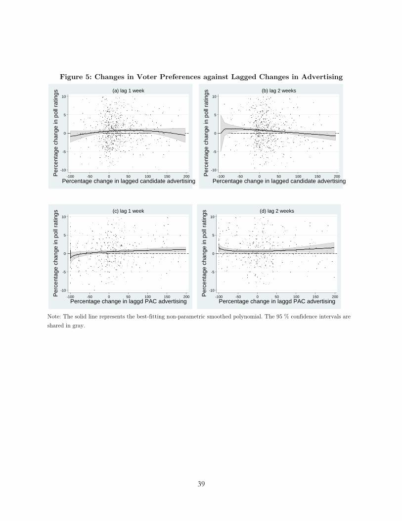
39

Figure 5: Changes in Voter Preferences against Lagged Changes in Advertising

Note: The solid line represents the best-fitting non-parametric smoothed polynomial. The 95 % confidence intervals are shared in gray.

-10

-5

0

5

10

Per

cent

age

chan

ge in

pol

l ra

tings

-100 -50 0 50 100 150 200

Percentage change in lagged candidate advertising

(a) lag 1 week

-10

-5

0

5

10

Per

cent

age

chan

ge in

pol

l ra

tings

-100 -50 0 50 100 150 200

Percentage change in lagged candidate advertising

(b) lag 2 weeks

-10

-5

0

5

10

Per

cent

age

chan

ge in

pol

l ra

tings

-100 -50 0 50 100 150 200

Percentage change in laggd PAC advertising

(c) lag 1 week

-10

-5

0

5

10

Per

cent

age

chan

ge in

pol

l ra

tings

-100 -50 0 50 100 150 200

Percentage change in laggd PAC advertising

(d) lag 2 weeks